Article

An Adaptive Scheme for Neuron Center Selection to Design an Efficient Radial Basis Neural Network Using PSO

Department of Mechanical and Robotics Engineering, Gwangju Institute of Science and Technology, Gwangju 61005, Republic of Korea
Mathematics 2026, 14(3), 469; https://doi.org/10.3390/math14030469
Submission received: 29 December 2025 / Revised: 20 January 2026 / Accepted: 24 January 2026 / Published: 29 January 2026
(This article belongs to the Section E: Applied Mathematics)

Abstract

An adaptive and efficient particle swarm optimization (PSO)-based learning algorithm to determine neuron centers in the hidden layer of a radial basis neural network (RBNN) is developed in the present work for regression problems. The proposed PSO–RBNN algorithm searches the entire input domain space to discover optimal neuron centers by solving an optimization problem and aims to overcome the limitation of center selection from the training data. The network is built in a sequential manner using optimal neuron centers until some specified criterion is met, and therefore, it exploits the concept of neuron significance during the learning process. The Gaussian function with a constant spread (also known as width) is chosen as the radial basis function for each neuron. To illustrate the effectiveness of the PSO–RBNN algorithm over the orthogonal least squares (OLS) method (a popular learning algorithm under a similar category, which selects the neuron center from training data), numerical simulations for different types of nonlinear problems of varying dimensions and complexities are conducted. Finally, a comparison with multiple existing algorithms for network design is made using available data. The results show that the RBNN architecture developed with the proposed learning algorithm exhibits superior convergence, displays good generalization ability, and requires a smaller number of neurons, resulting in an efficient and compact network architecture.

1. Introduction

Radial basis neural networks (RBNNs) have been applied to solve a variety of classification and regression problems in science and engineering [1,2,3,4,5,6]. The motivation for the use of an RBNN comes from its simple architecture (a three-layer feed-forward network), strong generalization ability, and ease of implementation. A survey of open literature suggested that an RBNN is a good choice for function approximation for multi-variate regression problems under the condition that a sufficient number of neurons are provided [7].
One of the key requirements for developing an RBNN model is to determine the number of neurons in the hidden layer—the center of each neuron—and a design variable that controls the sensitivity of radial basis neurons, also known as a spread constant. Once the network architecture is fixed, the weights and biases in the linear layer can be determined by solving a least-squares problem on training data. A variety of approaches have been proposed for the optimum selection of the network parameters, i.e., number, centers, and spread, either separately or in tandem.
A simple method to build a reasonable network is to take a number of neurons equal to the size of the training set and place them on the locations of the training data points [8]. However, the method is impractical for large datasets as it results in an excessively large number of neurons in the hidden layer. To avoid this problem, representatives of clusters of the data points can be found using suitable clustering techniques, and the neurons can then be placed at the locations of the obtained clusters. This will significantly reduce the number of neurons compared to when the entire training dataset is used.
Lee and Rhee [9] proposed training algorithms based on supervised hierarchical clustering methods. Web and Shannon [10] investigated different types of basis functions for regression and discrimination analysis and presented an iterative strategy to obtain the functional form using the conjugate-gradient method. In their investigation, the choice of neuron centers was made using the k-means clustering method. Among the different clustering algorithms, k-means clustering [11], an iterative method for forming clusters, became very popular for the choice of neuron centers [10].
Another approach to choosing neuron centers as a subset of training data was proposed by Chen et al. [12] and was based on the orthogonal least squares method (OLS). The OLS method is used to identify subsets of fixed functions of the inputs (regressors), which can explain maximum variance in the output. They suggested that each center corresponds to a given regressor in a linear regression model, and therefore, OLS learning can be regarded as the problem of finding neuron centers. The algorithm automatically determines the number and form (location of centers) of the hidden-layer neurons, considering both the performance and the complexity of the network. A regularized forward selection (RFS) method was introduced by Orr [13], which used subset selection and regularization to improve the generalization ability of the RBNN model. Chen et al. [14] presented a regularized orthogonal least square (ROLS) learning method, which combined the advantages of the OLS and regularization to provide efficient RBNN models with better generalization compared to the ordinary OLS method.
Evolutionary algorithms have been used by many researchers to tune network parameters and develop optimal RBNN architecture for classification as well as regression problems [15,16,17,18,19]. Qasem et al. [15] presented several multi-objective evolutionary hybrid algorithms to design radial basis function network (RBFN) for multi-class pattern classification problems. The algorithms were the memetic Pareto particle swarm optimization-based RBFN (MPPSON), Memetic Elitist Pareto non-dominated sorting genetic algorithm-based RBFN (MEPGAN) and Memetic Elitist Pareto non-dominated sorting differential evolution-based RBFN (MEPDEN). The proposed methods design RBFNs with a proper balance between accuracy and simplicity.
Billings and Zheng [16] used genetic algorithm (GA) to automatically configure the network parameters. Akaike’s information criterion (AIC) was used as the objective function to balance the trade-off between network performance and network complexity. Oh et al. [17] applied Particle Swarm Optimization (PSO) and Differential Evolution (DE) to design an advanced architecture of k-means clustering-based polynomial Radial Basis Function Neural Networks (p-RBF NNs). The inputs to the PSO algorithm were the centers obtained from k-means clustering and the spread parameters, and the objective was to minimize the weighted least square error estimation (WLSE) function. It was found that PSO resulted in a better RBNN model compared to DE.
Alexandridis et al. [18] presented an algorithm for training RBNN based on nonsymmetric variant of the Fuzzy means (FM) algorithm to determine the number and locations of neuron centers. PSO was used to optimize fuzzy partition of the input space. The PSO-assisted nonsymmetric Fuzzy means (PSO–NSFM) showed better performance compared with the original symmetric Fuzzy means (SFM) algorithm. Han et al. [19] proposed a growing and pruning algorithm for radial basis function (RBF) neural network, named the self-organizing RBF (SORBF) method, for function approximation and dynamic system identification. In the SORBF algorithm, the network structure needs to be updated after pruning or the addition of neurons. The results indicated a better performance of SORBF algorithm compared with other algorithms for RBF network design. Feng [20] and Han et al. [21] employed PSO and adaptive PSO algorithms, respectively, to develop SORBF neural networks for solving nonlinear problems. In these studies, an optimization problem was formulated based on user-defined objective functions [20,21], and the design variables were taken to be the number, widths and centers of neurons as well as associated weights in the hidden layer. Using PSO algorithm, the network inputs were optimized, simultaneously. The authors demonstrated good prediction accuracy for some selected problems, but the number of input parameters to the PSO algorithm could be sufficiently large for high-dimensional problems.
The design of RBFNN architecture requires proper selection of the number and centers of hidden layer neurons, as well as the spread constant. Given sampled training data, the aim is to minimize the training error, and at the same time achieve improved generalization performance. The unsupervised learning approach using the k-means algorithm has several intrinsic disadvantages. First, the number of neurons needs to be specified by the user, and the algorithm does not automatically determine neuron centers. Second, the k-means algorithm is locally convergent, and the initial guess affects the choice of centers. This results in a time-consuming trial-and-error method to establish the size as well as the form of the hidden layer. The OLS learning algorithm [12,13,14], which is a popular method to determine neurons centers, suffers from the limitation of the available training data for center selection (significant regressors). A major limitation of above methods is that the neurons centers are chosen from the training data, and therefore, the resulting network may not be necessarily optimal. In practice, it is quite possible that the optimal neuron centers may not necessarily be from the training data but lie outside it. From possible proposed solutions using evolutionary techniques, the methods of Oh et al. [17] and Alexandridis et al. [18] do not operate on the training data directly but require additional algorithms (k-means clustering in Oh et al. 2012 [17] and FM algorithm in Alexandridis et al. 2013 [18]) to determine representatives of the data for optimization.
In view of these issues and challenges on the development of efficient neural network architecture, a PSO-based efficient learning algorithm to find neurons centers of the RBF NN model with a Gaussian basis function is proposed in the present work. The global search ability of PSO is exploited to determine the optimal centers outside the training data, and the obtained centers were added sequentially to develop the network architecture. The mean-squared error (MSE) on the training set was selected as the objective function and minimized using PSO. Simulations using available test problems were conducted to show the applicability of the proposed PSO–RBNN algorithm, and the results of comparative performance evaluation, in terms of convergence, required number of neurons, and generalization ability with existing algorithms, are presented.
The paper is structured as follows. Section 2 describes the RBNN architecture, Gaussian function, and mathematical formulation. A brief introduction to the PSO algorithm is provided in Section 3. The details of the proposed PSO–RBNN algorithm, and its implementation, is discussed in Section 4. Performance analysis results from numerical experiments using test problems and direct comparison to the OLS learning method and different existing algorithms are presented throughout Section 5 in the paper. Finally, Section 6 summarizes the conclusions, and ties up some loose ends for future research.

2. Radial Basis Neural Networks (RBNN)

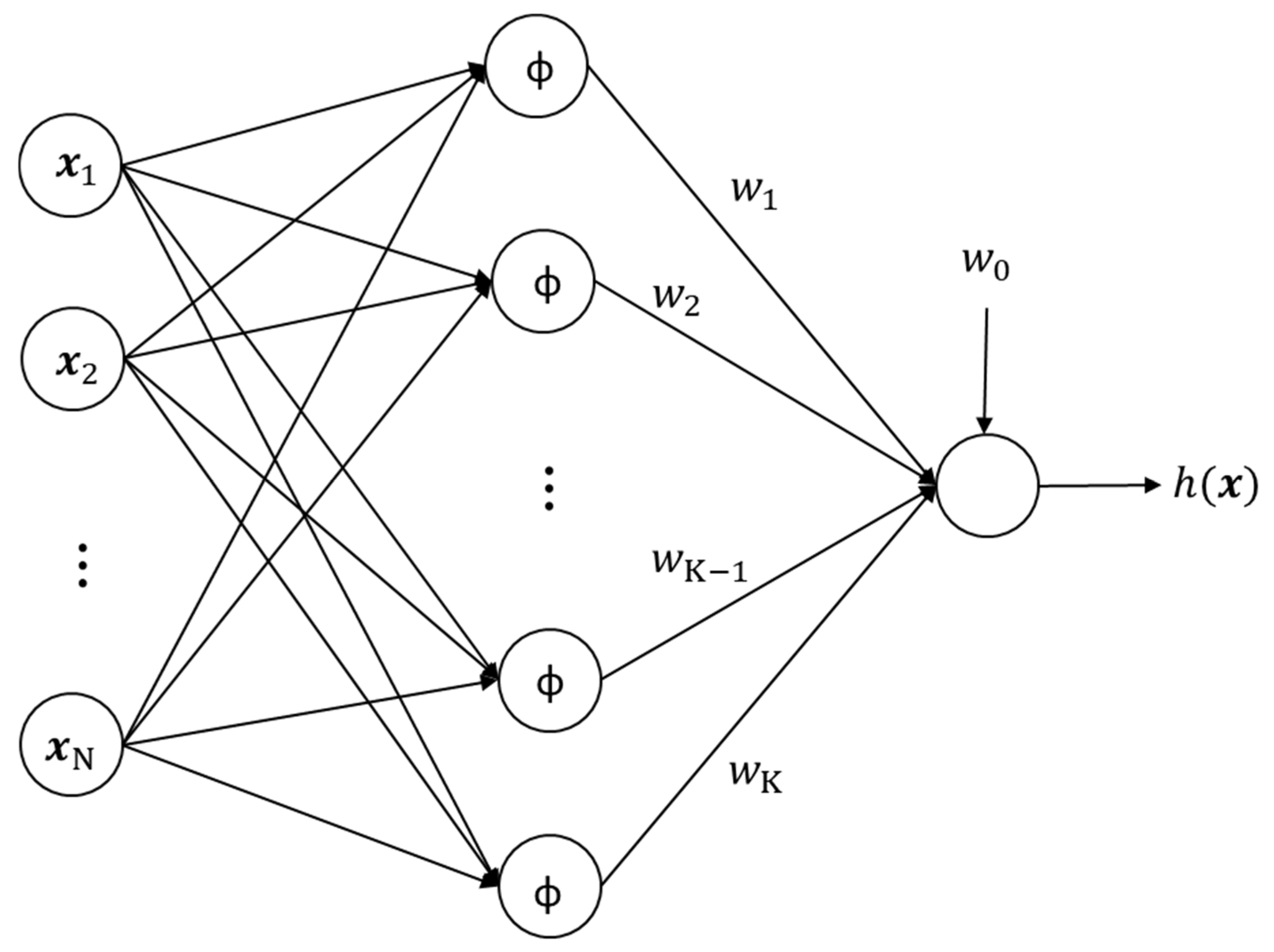
A typical RBNN architecture is shown in Figure 1. The architecture of RBNN consists of an input layer, a hidden layer of radial basis neurons and an output layer of linear neurons. Each layer is fully connected to the one following. The radial basis functions act as processing units between the input and output. The hidden layer performs a non-linear transformation of the input space to an intermediate space using a set of radial basis functions. The different types of radial basis functions (RBF) are: (1) Gaussian function, (2) multiquadratic function, (3) thin–plate–spline function, and (4) inverse multiquadratic function.
The details on the exact functional form of the different RBFs can be found in Web and Shannon [10] and Billings and Zheng [16]. Among the available basis functions, the Gaussian function is the most widely used and is implemented in the present work.
A Gaussian function of the following form is used as a transfer function for a radial basis neuron (RBN):
φ x = e x p   ( θ x c i 2 )
Each neuron in the hidden layer has an associated center c i and parameter θ which controls the sensitivity of the neurons (hereinafter referred to as the spread constant). The net input to the transfer function is the Euclidean distance x c i   between the neurons center c i and the input vector, x multiplied by θ . The Gaussian function is symmetric and can be regarded as a measure of similarity between the input vector x and center c i . For a fixed value of θ , the Euclidean distance x c i   governs the output of the Gaussian function; the greater the similarity between the input and center (lower Euclidean distance), the higher the output of the Gaussian activation function, and vice versa.
The inputs to the output layer are combined using a set of weights to produce the desired output, h x which can be expressed as:
h x = i = 0 K w i e x p   ( θ x c i 2 )  
Here, i = 0 denotes the bias w 0 and K is number of neurons in the hidden layer. The weights w i are obtained using training data ( x i ,   y i ; i = 1 ,   N ) by solving a linear least squares problem for the following objective function:
E T r a i n = 1 N i = 1 N h x i y i 2  
After fixing the network architecture (number of neurons in the hidden layer, their centers and spread constant), the weights w =   w 1 , w 2 , ,   w K ,   w 0 T can be expressed in the following matrix form:
w = ( X T X ) 1 X T Y
X = e x p   ( θ x 1 c 1 2 ) e x p   ( θ x 1 c K 2 ) 1 e x p   ( θ x 2 c 1 2 ) e x p   ( θ x 2 c K 2 ) 1     e x p   ( θ x N c 1 2 ) e x p   ( θ x N c K 2 ) 1 ,   Y = y 1 y i y N
where X is known as design matrix of the system, and Y is vector of outputs. Equation (4) can be re-written as:
w = X Y
where
X = ( X T X ) 1 X T
X is known as pseudo-inverse of X , and is determined using singular-value decomposition (SVD) in the present study.

3. Particle Swarm Optimization

PSO is an evolutionary optimization algorithm developed by Kennedy and Eberhart [22]. It is inspired by the movement of bird flock or fish schools. Particle swarm optimization starts with an initial population of possible solutions (particles) with some initial velocities, all randomly generated. A particle refers to a point in the hyperdimensional search space that iteratively changes its location based on the velocity updates. At the start of iteration, the fitness function value at each particle position, and the best function values and corresponding positions, are determined. In the iteration loop, the new velocities for all particles in the swarm are updated based on their current velocities, particle best (particle individual optimal positions) and global best (best particle position in the swarm) using a weighted approach, and some parameters. The particle positions are then updated using the new velocities for the next iteration. These steps are repeated until the desired stopping criterion is reached. PSO is a conceptually simple, easy-to-implement, and computationally efficient algorithm with a well-balanced mechanism to enhance global exploration and local exploitation abilities. Compared to other evolutionary algorithms, such as GA and DE, PSO is capable of achieving faster convergence while maintaining sufficient solution accuracy [23].

4. PSO–RBNN Algorithm

The optimization problem to determine neuron centers c R d in the hidden layer of RBNN can be formulated as follows:
min c R d E T r a i n ,   L B i   c i U B i   ( i = 1,2 , ,   d )
Here, L B i and U B i are the lower and upper bounds for each input variable, respectively, and d is the dimension of the input space. However, using normalization on the training data, it is bounded between 0 and 1. Since the particle positions are generated from a uniform random distribution in the interval [0, 1], normalization provides computational convenience in the implementation. The PSO procedure was terminated when either the maximum number of iterations was reached or when the relative change in E T r a i n between two consecutive iterations fell below a predefined threshold value of 10−5. The PSO–RBNN algorithm is implemented as follows:
  • The inputs to the algorithm are training data ( x i ,   y i ; i = 1 ,   N ) , parameter θ and a tolerance value for the mean-squared error E T r a i n to terminate the algorithm. Initialize the neural network architecture with c 1 =   n   = 1 N x n , the mean of the training sample. Construct the matrix X , and determine the weights using Equation (4). Calculate E T r a i n using Equations (2) and (3).
  • Initialize PSO with a random population of size P , and assign each particle a position (neuron center) c j and velocity, v j ( j = 1 ,   2 , ,   P ) generated from uniform random distributions in [0, 1]. The objective function is E T r a i n , evaluated using Equation (3).
    P1.
    Update each particle position (neurons center) c j and velocity v j ( j = 1 ,   2 , ,   P ) at each iteration k using the following equations:
    c j k + 1 = c j k + v j k + 1
    v j k + 1 = ω v j k + a 1 r 1 p j k c j k + a 2 r 2 p g k c j k
    where a 1 and a 2 are acceleration coefficients, the vector p j is known as the personal best position for each particle, and the vector p g is known as the global best position in the population evaluated using a criterion based on the fitness function [20]. The parameters r 1 and r 2 are random numbers in the range [0, 1] sampled from a uniform normal distribution. Shi & Eberhart [23] introduced the parameter ω , known as inertia weight, which is commonly used to accelerate the convergence speed of the algorithm. A moderate swarm size (15 × number of variables) was employed to balance solution diversity and computational cost, while the inertia weight and acceleration coefficients were selected according to standard PSO guidelines to ensure stable convergence. The values of the acceleration coefficients a 1 , a 2 , and the inertia weight ω were taken from Shi & Eberhart [23]. The value of a 1 , a 2 and ω was set to 2.0, 2.0 and 1.1, respectively.
    P2.
    Enforce the bounds on particle positions, and velocities.
    P3.
    The personal best position for each particle in the population can be updated
    p j k + 1 = c j k + 1   i f   f c j k + 1   f c j k c j k   i f   f c j k + 1 < f c j k
    P4.
    The global best at each iteration, k is calculated as the best among the personal best positions:
    p g k + 1 = min p j k + 1 f ( p j k + 1 )
  • After the PSO algorithm terminates, the network architecture is appended with the center which is the global best solution obtained from step 2. Construct the matrix X , and determine the weights using Equation (4). Calculate E T r a i n using Equations (2) and (3).
  • Repeat step 2 to generate new centers, until the mean-squared error E T r a i n is less than the specified tolerance or maximum number of neurons reached (size of training set).

5. Results and Discussion

5.1. Numerical Simulations and Performance Comparison

Numerical experiments were carried out to test the performance of the proposed PSO–RBNN algorithm in terms of convergence, model complexity and generalization ability; convergence and model complexity were gauged using MSE on the training set (Equation (3)), and a suitable test set was used to assess generalization ability. A MATLAB R2020b code for the PSO–RBNN algorithm was developed and tested on different types of analytical test problems involving real-valued functions [24]. The test functions were chosen to cover problems with varying dimensions and complexity. The functional forms of the test problems are given as follows:
  • One-dimensional Function
    f ( x ) = x s i n ( x )
    where 0 x i 10 .
  • Booth Function
    f x = ( x 1 + 2 x 2 7 ) 2 + ( 2 x 1 + x 2 5 ) 2
    where 10 x i 10 , i = 1 , 2 .
  • Six–Hump Camel Back Function
    f x = 4 2.1 x 1 2 + x 1 4 3 x 1 2 + x 1 x 2 + ( 4 x 2 2 4 ) x 2 2
    where 5 x i 5 , i = 1 , 2 .
  • Hartmann 3 Function
    f x = i = 1 4 a i   e x p j = 1 3 b i j ( x j d i j 2
    where 0     x j   1 ,   j     1 ,   2 ,   ,   3 . a =   1 ,   1.2 ,   3 ,   3.2 T , and b and d are given by
    b = 3.0 10 30 0.1 10 35 3.0 10 30 0.1 10 35 ,   d = 0.3689 0.1170 0.2673 0.4699 0.4387 0.7470 0.1091 0.8732 0.5547 0.03815 0.5743 0.8828
  • Hartmann 6 Function
    f x = i = 1 4 a i   e x p j = 1 6 b i j ( x j d i j 2
    where 0     x j   1 ,   j     1 ,   2 , , 6 . a =   1 ,   1.2 ,   3 ,   3.2 T , and b and d are given by
    b = 10.0 3.0 17.0 3.5 1.7 8.0 0.05 10.0 17.0 0.1 8.0 14.0 3.0 3.5 1.7 10.0 17.0 8.0 17.0 8.0 0.05 10.0 0.1 14.0
    d = 0.1312 0.1696 0.5569 0.0124 0.8283 0.5886 0.2329 0.4135 0.8307 0.3736 0.1004 0.9991 0.2348 0.1451 0.3522 0.2883 0.3047 0.6650 0.4047 0.8828 0.8732 0.5743 0.1091 0.0381
The training, validation and test data sets were generated using the Latin hypercube sampling (LHS) technique [25,26]. LHS is a widely used design-of-experiment (DOE) procedure used by many researchers, owing to its better space-filling property, sample flexibility and small sample sizes. In the present study, lhsdesign (MATLAB built-in function for LHS) was used to generate the sample points with the criterion ‘maximin’ (maximize the minimum distance between points). It is an iterative method that generates LHS samples at random and chooses the best one based on the criterion ‘maximin’. To construct the experimental design (sample), the number of sample points is specified by the user.
Table 1 presents the details of the test functions and the corresponding data sets used in the present study. The numerical experiments were performed using a computer with an Intel Core i7 processor (assembled, Seoul, Republic of Korea) with four CPUs, 16 GB RAM, and a clock speed of 3.40 GHz in serial processing mode. Furthermore, a direct comparison of the PSO–RBNN algorithm with OLS learning (a well-known learning algorithm for RBF NN modeling) proposed by Chen et al. [12] was conducted. For both methods, the network parameters, including the number and locations of neurons, were determined using the training dataset, while the optimal model selection with respect to the spread constant θ was performed using the validation dataset. This validation-based selection prevents the network from overfitting the training data and improves the generalization performance of the network. Finally, the predictive performance of each model was then assessed using an independent test dataset.
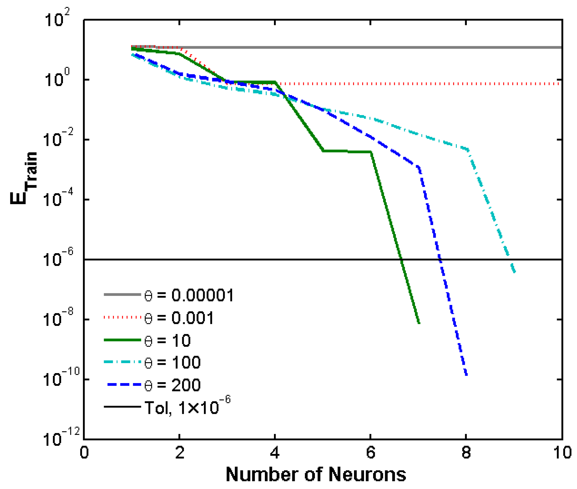
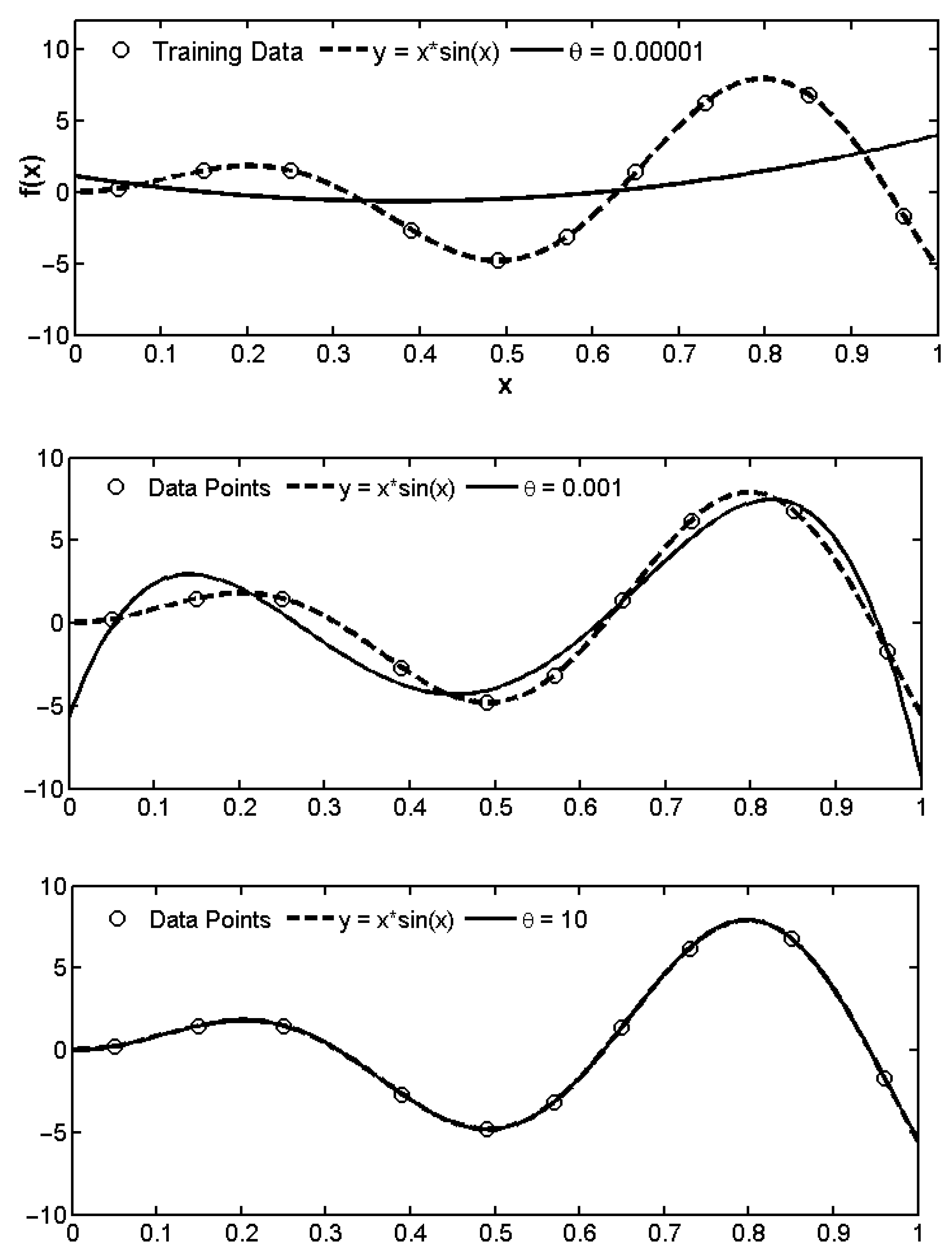
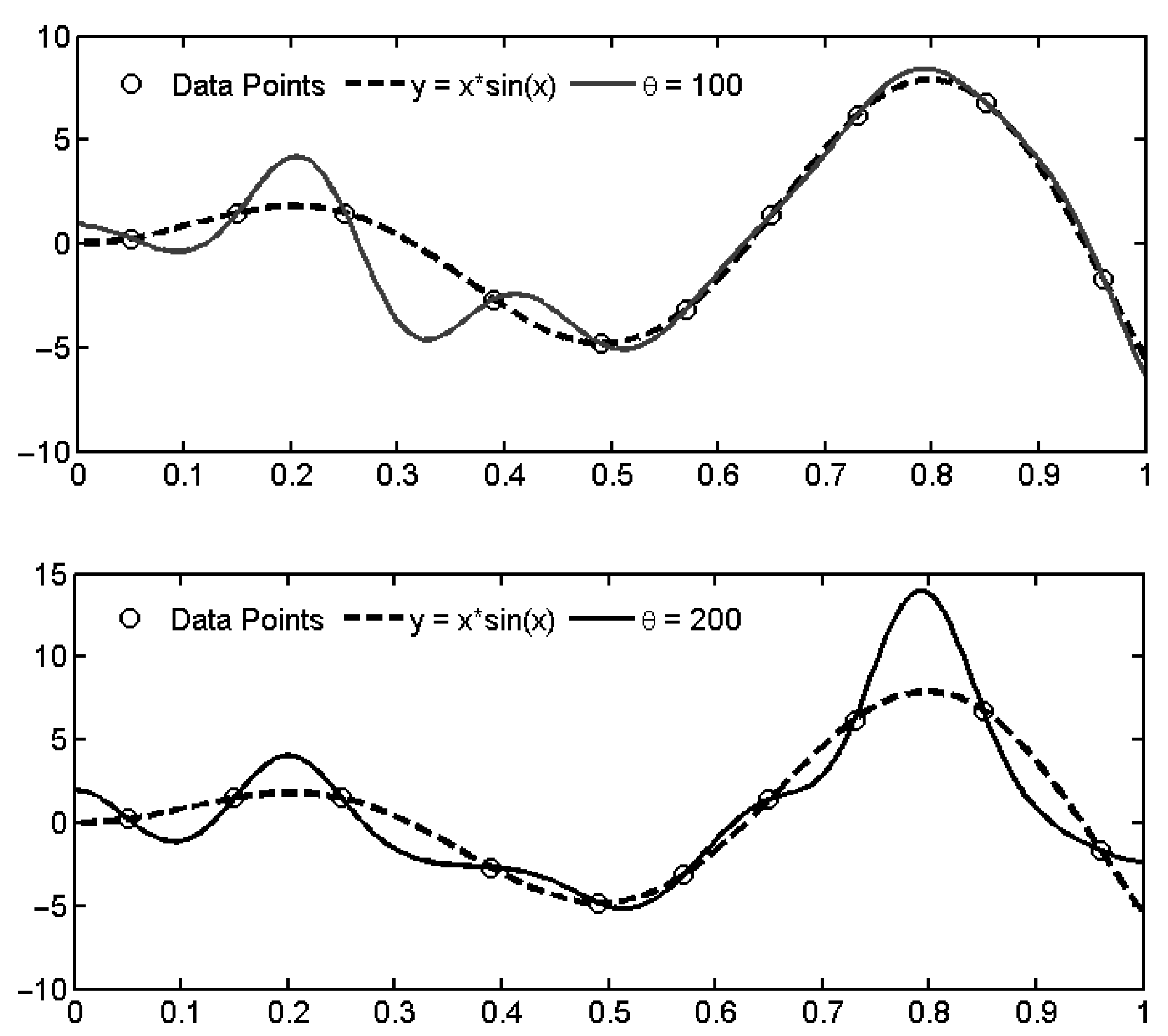
Figure 2 shows the evolution of training error with the number of neurons for a 1D function at different values of the spread constant, while the corresponding function approximations are shown in Figure 3. This exercise was conducted to illustrate under- and over-fitting behavior associated with the choice of spread constant using the PSO–RBNN algorithm. For small values of the spread constant ( θ = 0.00001 and 0.001), underfitting will occur due to the large overlapping of the neurons, which leads to an ill-conditioned design matrix, X in Equation (4). In such cases, the SVD uses low-rank approximation for X to compute the linear weights, resulting in smoother approximation and reduced model flexibility.
As can be seen from Figure 2, the network performs poorly on training data and is not able to reach the desired error goal. In contrast, for higher values of spread constant ( θ = 100 and 200), overfitting becomes a serious issue (the network performs very well on the training set but exhibits poor generalization ability). The neuron output is limited to a narrow range and dies out very quickly. At the optimal spread constant ( θ = 10), the overlap is within a certain level, resulting in sufficiently accurate approximation. Therefore, although the PSO–RBNN algorithm selects the centers from the input domain using optimization of the mean-squared error, E T r a i n , the choice of spread constant has a significant influence on the solution. Consequently, model validation strategies, viz., validation set or cross-validation, are required for model selection as in other existing learning algorithms.
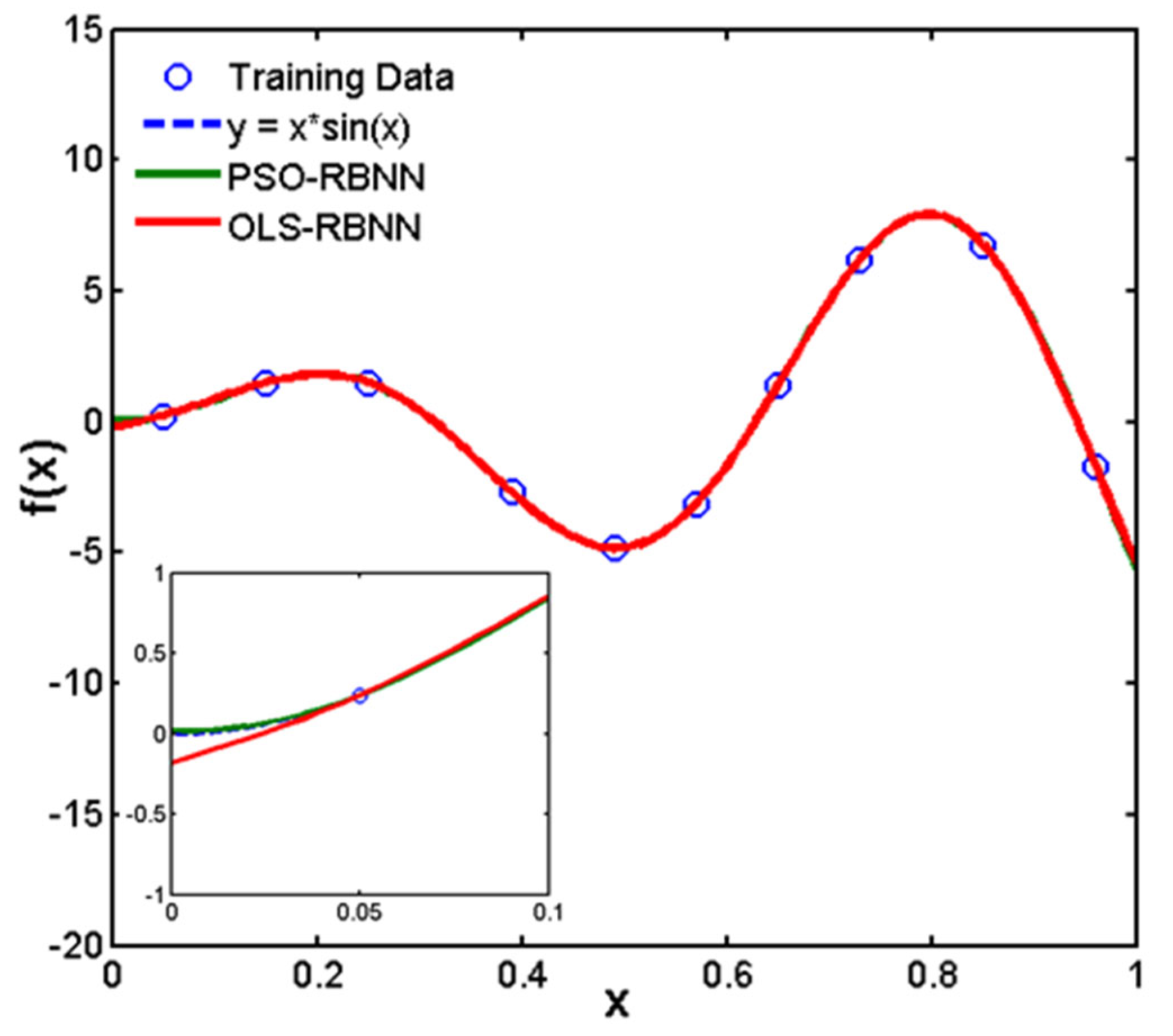
Table 2 lists the neuron centers and training error as both algorithms proceed towards convergence for the 1D function. As mentioned earlier, the optimum spread constant was found using a validation set for both the methods. The OLS–RBNN method selects the neuron centers directly from the training data, whereas the PSO–RBNN searches the input space to determine the optimum centers. As a result, the PSO–RBNN exhibits faster convergence and requires less neurons, as depicted in Table 2. Figure 4 shows a comparison of the prediction accuracy between neural networks trained using the PSO–RBNN and OLS–RBNN algorithms.
The model performance with both the learning algorithms was found to be good, but the PSO–RBNN showed a slightly better prediction accuracy compared to the OLS–RBNN near the lower bound on the input variable, as shown in Figure 4.
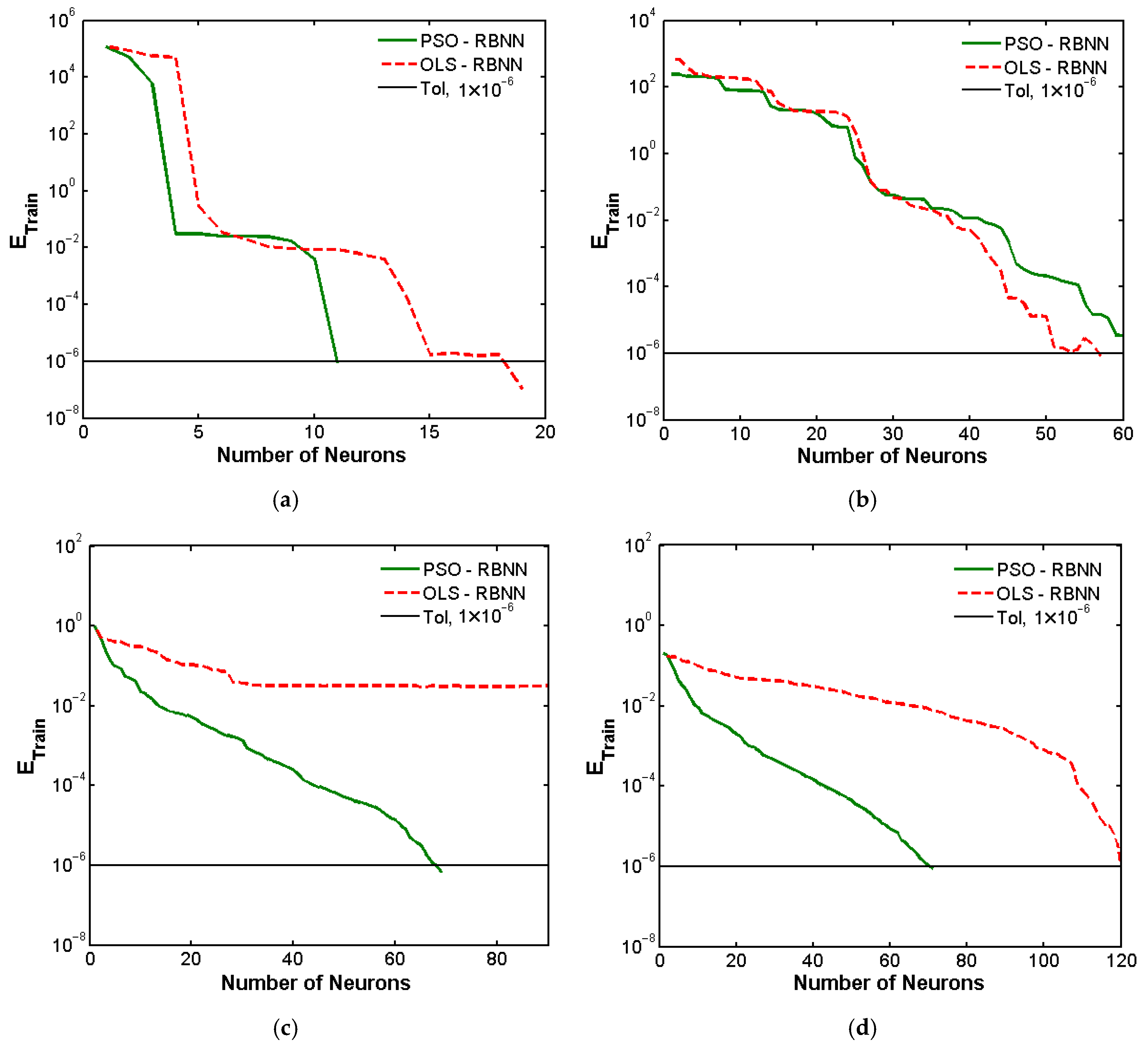
The evolution of training error with number of neurons—added to the network in a sequential manner—for the PSO–RBNN algorithm is shown in Figure 5 and compared with the OLS method. The PSO–RBNN algorithm was simulated 20 times using the data sets for the test problems, and the best result, based on the validation and test data, was used for comparison. For most of the selected test problems, the PSO–RBNN algorithm outperforms the OLS–RBNN, except for the six-hump camel back function where it is slightly worse than the OLS method. In fact, the PSO–RBNN outperforms the OLS–RBNN right from the selection of the first neuron center, highlighting the efficacy of the PSO–based search strategy proposed in the present work. For Booth, Hartmann 3 and Hartmann 6 functions, a faster convergence behavior is observed for the PSO–RBF NN algorithm compared to the OLS–RBNN and significantly lower number of neurons is also required. For Hartmann 3 function, the OLS method fails to reach the specified error goal on the training set with a sufficiently large discrepancy whereas the PSO–RBF NN attains fast convergence as shown in Figure 5c. The decreases in the number of neurons selected by the PSO–RBNN algorithm are found to be 36.84%, 22.21% and 41.67% for the Booth, Hartmann 3 and Hartmann 6 functions, respectively, compared with the OLS–RBNN algorithm.
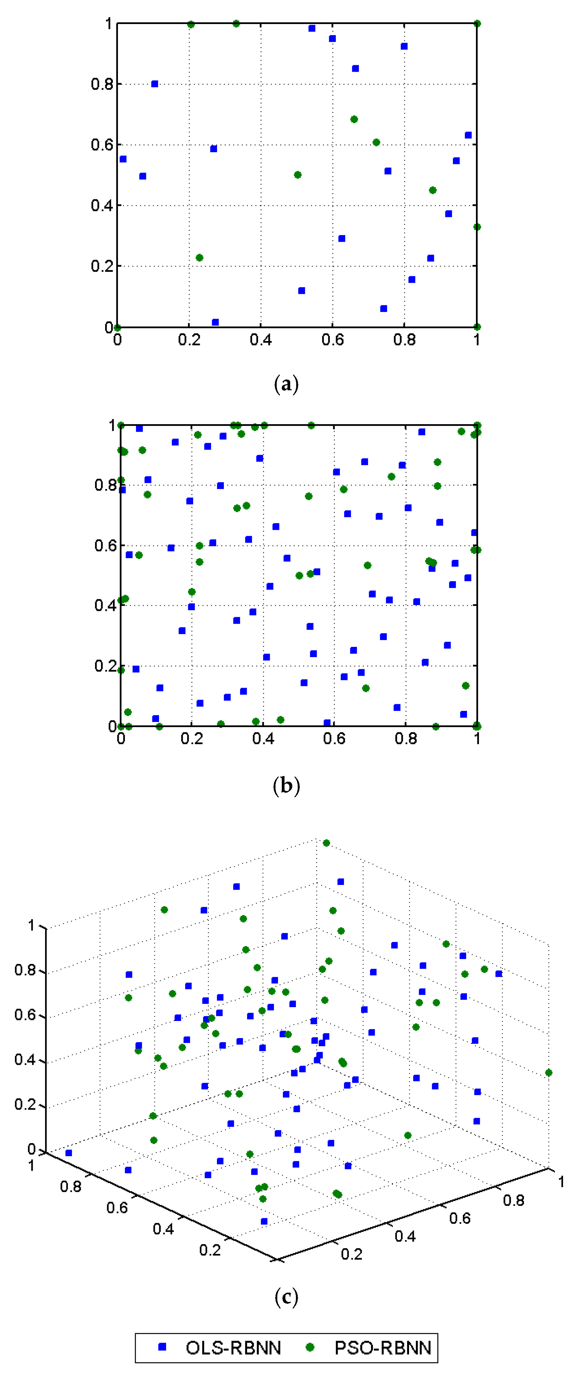
Figure 6 shows the distribution of neuron centers in the input domain obtained using the PSO– and OLS–RBNN algorithms for the optimal network structure. The neurons centers were obtained from the training data for the OLS method, whereas PSO was used to scan the entire space of the input variables to select the centers, as shown in Figure 6; the neurons centers were not from the training points but selected randomly from the input domain based on the proposed PSO–RBNN algorithm. Localized clusters of neuron centers can be seen, which can be attributed to the fact that more centers are required in the regions where the variation in the objective function, E T r a i n given by Equation (3), is expected to be large.
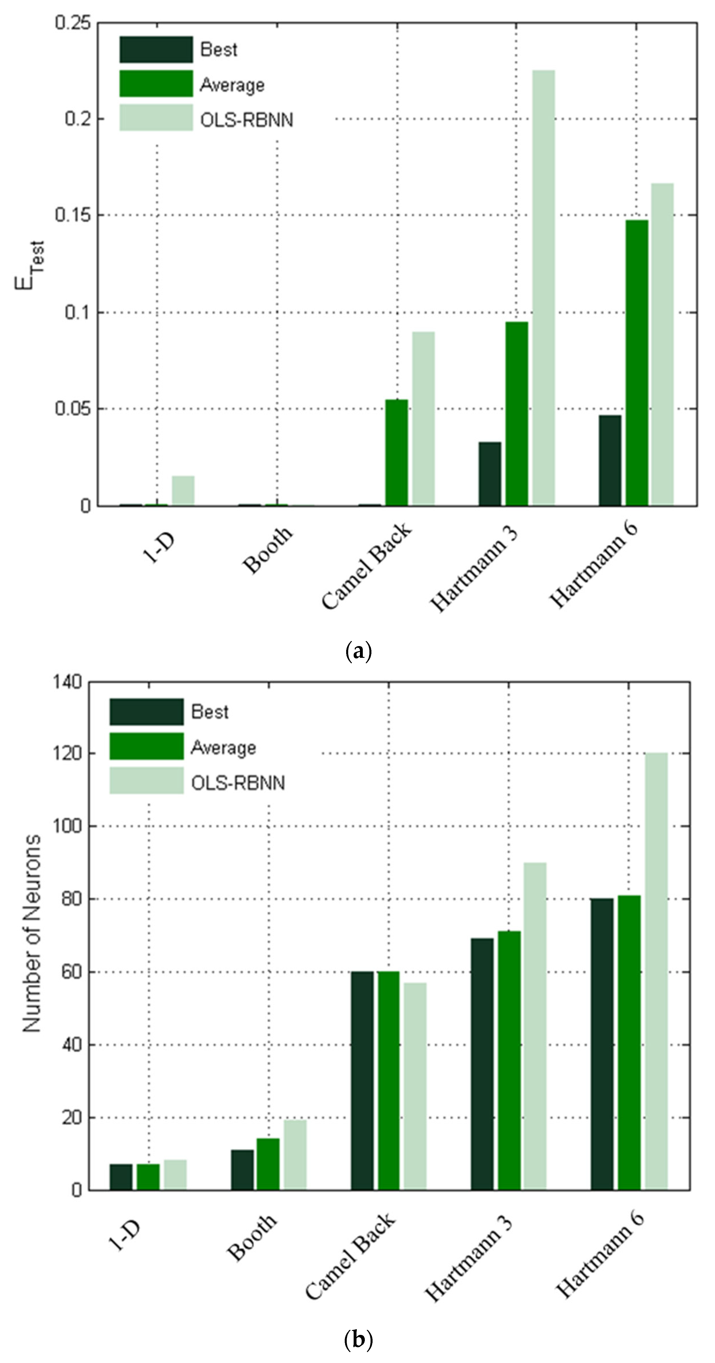
Figure 7 presents the mean-squared error on the test set, E T e s t , and the total number of selected neurons for the PSO–RBNN and OLS–RBNN algorithms. A comparison of the test error indicates superior generalization ability of the network trained by the PSO–RBNN algorithm, both in terms of the best outcome as well as the overall average across multiple trials as shown in Figure 7a for all test problems. Interestingly, the best test error for the six-hump camel back function from the PSO–RBNN is found to be considerably lower than the OLS algorithm. Consequently, a slightly worse performance in the training is offset by a remarkable increase in the generalization ability of the network, which is important in the context of learning because the generalization error is the bottom line, not the training error. The training convergence curve shown in Figure 5a corresponds to the trial yielding the minimum test error, since faster convergence was observed in some runs to coincide with poorer generalization. Furthermore, the PSO-RBNN requires a significantly lower number of neurons in comparison with the OLS–RBNN to develop the optimal network structure for all tested problems, except for the six-hump camel back function as shown in Figure 7b. Thus, the PSO–RBF NN shows the best overall performance, namely learning and generalization, compared to the OLS method. Also, the PSO–RBNN algorithm tends to produce simpler models with a smaller number of parameters (number of neuron centers and weights in the linear layer).
As mentioned earlier, the PSO–RBNN algorithm was run 20 times using the data sets for the test problems, and therefore, the mean and standard deviations were computed. The training and test errors, together with the number of neurons, are summarized in Table 3. The standard deviation for training error and number of neurons is found to be small, yielding a consistent network architecture, but different level variations in the test error are observed depending on the test problem; maximum variation is observed for the six-hump camel back function. Nevertheless, for the best model selection, one of the advantages of the variability in the generalization ability of the PSO–RBNN algorithm is that one can make a choice of a very good model from a candidate pool of well-performing models.
PSO has been used previously by different authors to develop RBNN architecture, and therefore, the predictive performance and convergence properties of the proposed PSO–RBNN algorithm are compared with two popular existing algorithms, PSO–NSFM by Alexandridis et al. [18] and pRBF NN by Oh et al. [17]. To compare with the PSO–NSFM algorithm, two test problems were selected as follows:
  • Friedman [25]
    y = 5 2 s i n π x 1 x 2 + 4 x 3 0.5 2 + 2 x 4 + x 5 +
    where 0 x i 1 and   is a Gaussian noise ~ N(0, 0.8).
  • Samad [26]
    y = 1 1 + exp [ exp x 1 + x 2 0.5 2 + s i n π x 3 ]   +
    where 0 x i 1 and   is a Gaussian noise ~ N(0, 0.025).
For each case, the data were split randomly for training (50%), validation (25%) and testing (25%) subsets, following the procedure of Alexandridis et al. [18]. Table 4 compares the root mean squared error (RMSE) for the validation and test sets between PSO–RBNN and PSO–NSFM, together with the corresponding number of hidden neurons. It can be observed that the proposed PSO–RBNN consistently achieves lower or comparable RMSE values relative to PSO–NSFM, while requiring a significantly smaller network size. This reduction in the number of neurons indicates improved parsimony without compromising predictive accuracy. The results confirm that the direct optimization of RBF centers using PSO, combined with least-squares weight estimation, provides strong generalization capability on chose nonlinear benchmark problems.
An additional study was conducted to examine the effect of training sample distribution and noise characteristics on the generalization performance of the PSO–RBNN algorithm. The results, averaged over 20 independent trials, are summarized in Table 5 for two cases: noise-free data with noisy data generated from a specified Gaussian distribution. For both the Friedman [27] and Samad [28] datasets, the PSO–RBNN exhibits low RMSE values in noise-free cases, confirming its strong generalization ability. When noise is introduced, an expected increase in RMSE is observed; however, a reasonable and controlled adjustment in the number of neurons and generalization error was evident in both cases, reflecting the adaptive nature of the proposed learning strategy.
The robustness of the PSO–RBNN algorithm to noise was further investigated using different Gaussian noise distributions, as reported in Table 6. Although the presence of noise leads to higher prediction errors, the overall increase in RMSE remains moderate, indicating stable learning behavior. Importantly, the network size does not increase excessively under noisy conditions, demonstrating that the proposed approach avoids overfitting and maintains a compact network structure even when the data are corrupted by stochastic disturbances. These results collectively highlight the robustness of PSO–RBNN with respect to variations in both noise level and training sample distribution, owing to its adaptive center selection and validation-based control of model complexity.
For comparison with the pRBF NN algorithm, two real-world datasets, (a) Automobiles miles per gallon (MPG), and (b) Boston housing, were used. Each dataset was randomly split into training (60%) and testing (40%) subsets, following the procedure of Oh et al. [17]. Table 7 compares the root mean squared error (RMSE) values obtained on the training and test sets for the PSO–RBNN and pRBF NN. The PSO–RBF NN algorithm demonstrates superior generalization ability but requires more neurons compared to the pRBF NN approach. However, the overall computational effort for PSO–RBNN is significantly lower than pRBF NN, as the latter involves additional computation of polynomial coefficients.
Finally, a 1D function [29] commonly used in different research works is used in the present study to compare the performance of the present PSO–RBF NN algorithm with the existing algorithms such as DFNN [30], GA–RBF [29] and SO–RBF [19]. The function form is as follows:
f x = 0.8 × e 0.2 x × s i n ( 10 x )
The size of the training and test samples was set to 200, each obtained using LHS, and randomly distributed in the interval [0, 2]. Table 8 shows the detailed results of the comparison of different algorithms. The present PSO–RBF NN algorithm showed significant improvement in the generalization ability and required a lower number of neurons compared with the given existing algorithms.


5.2. Computational Complexity

The computational complexity of the PSO–RBNN algorithm can be determined from the individual complexities of the PSO procedure and the least-squares problem. For a training sample of size n and input dimension d , the computational complexity of PSO per iteration is O ( P d ) , where P denotes the swarm size. In the proposed PSO–RBNN framework, the fitness evaluation involves computing the RBF activations and solving a least-squares problem to estimate the output weights. The cost of computing RBF activations is O ( n d ) , while the cost of solving the least-squares problem for k hidden neurons is O ( n k 2 + k 3 ) . Hence, the total computational complexity of PSO per iteration is given by O ( P ( n d +   n k 2 + k 3 ) ) . If the PSO procedure is executed for N iterations to add a single neuron, the computational cost becomes O ( N P ( n d +   n k 2 + k 3 ) ) . Since the network is constructed sequentially by adding K neurons, the overall computational complexity of the PSO–RBNN algorithm is O k = 1 K N P ( n d +   n k 2 + k 3 ) . In our implementation, the dominant memory requirement is O n K for storing design matrix, and O ( P d ) for storing PSO particle states. In addition, the O ( K d ) memory is required to store the RBF center locations. Therefore, the space complexity is O ( n K + K d +   P d ) .
The training complexity of OLS–RBNN algorithm is O ( n K 2 + K 3 ) . Consequently, the PSO–RBNN incurs an additional cost proportional to swarm size and PSO iterations and the repeated solution of least-squares problems during fitness evaluation. Nevertheless, the additional computation results in significantly improved generalization performance and a smaller network size. Compared with PSO–NSFM, which optimizes a nonsymmetric fuzzy partition of the input space using PSO, the proposed PSO–RBNN directly optimizes RBF center locations and therefore incurs higher computational cost due to repeated least-squares solves during PSO iterations. However, the direct center optimization strategy adopted in PSO–RBNN provides greater flexibility in neuron placement and avoids restrictions imposed by predefined fuzzy partitions. This enhanced adaptability typically results in comparable or superior generalization performance while achieving smaller and more efficient network structures.

5.3. Case Study: Quantitative Estimation of Energy Performance of Residential Buildings

The final evaluation of PSO–RBNN performance was conducted using a real-world problem that requires accurate quantitative estimation of the energy performance of residential buildings [31]. The problem involves eight input variables, namely relative compactness, surface area, wall area, roof area, overall height, orientation, glazing area, glazing area distribution, and two response variables: heating load (HL) and cooling load (CL). The dataset consists of 768 samples, which were randomly divided into training (70%), validation (15%), and testing (15%) subsets for performance evaluation. To ensure fairness and avoid bias in the comparative analysis, 20 independent trials were performed, and the results are reported in terms of statistical performance measures, including the mean and standard deviation. Table 9 presents the mean squared error (MSE) obtained on the test dataset using the PSO–RBNN algorithm and provides a comparison with previously published results based on Iteratively Reweighted Least Squares (IRLS) and Random Forest (RF) methods. The PSO–RBNN model consistently outperforms IRLS and Random Forest (RF) for both heating load (HL) and cooling load (CL) prediction, achieving the lowest mean error and significantly reduced variability. This indicates the superior prediction accuracy and improved stability of the PSO–RBNN approach for residential building energy performance estimation.

6. Conclusions

In this paper, an efficient learning algorithm, referred to as the PSO–RBNN algorithm, was developed to determine neurons centers in the hidden layer of the RBNN model using PSO. The proposed algorithm performs a global search in the input domain space to determine optimal neuron centers by solving an optimization problem in which the mean-squared error on the training set is used as the objective function. The centers are added in a sequential order until the mean-squared error falls below a specified value, or the maximum number of neurons is reached (size of the training set). Although the neuron centers are optimized during the training stage, model selection was performed using a validation set to determine the optimal spread constant of the Gaussian function employed in this study. Numerical investigation carried out on selected test problems demonstrates that the PSO–RBNN algorithm can learn the underlying process (function) using data with sufficient accuracy. Also, a faster convergence, better generalization performance, lower number of neurons, and simple models were observed with the proposed PSO–RBNN algorithm compared with some of the existing algorithms for the design of RBNN architecture. In addition, the algorithm was found to be robust with respect to variations in training sample distribution and the presence of noise in the data. A case study on a real-world problem dataset reveals the superior performance of the PSO–RBNN algorithm compared with other statistical machine learning techniques. The proposed algorithm offers ease of implementation on any computing platform due to its simple structure. Future research aims to improve the robustness of the PSO–RBNN algorithm through the strategic selection of parameters used in the PSO algorithm and the investigation of alternative forms of radial basis functions.

Funding

This work was supported by the Department of Science and Technology (DST) grant, Government of India (Grant number: DST/INSPIRE/04/2016/000014). The author gratefully acknowledges this support.

Data Availability Statement

The original contributions presented in this study are included in the article. Further inquiries can be directed to the corresponding author.

Conflicts of Interest

The author declares no conflicts of interest.

Abbreviations

The following abbreviations are used in this manuscript:
PSOParticle swarm optimization
OLSOrthogonal least squares
RBFRadial basis function
LHSLatin hypercube sampling
GEGenetic algorithm
DEDifferential evolution
MSEMean squared error
AICAkaike’s information criterion
WLSEWeighted least square error
DFNNGeneralized fuzzy neural networks
SO–RBFSelf-organizing radial basis function
IRLSIteratively reweighted least squares
RFRandom forest

References

  1. Afzal, A.; Chung, H.; Muralidhar, K.; Cho, H.-H. Neural network assisted optimization of rectangular channels with intersecting ribs for enhanced thermal performance. Heat Transf. Eng. 2020, 41, 1609–1625. [Google Scholar] [CrossRef] [Scilit]
  2. Akhmetov, D.F.; Dote, Y.; Ovaska, S.J. Fuzzy neural network with general parameter adaptation for modeling of nonlinear time-series. IEEE Trans. Neural Netw. 2001, 12, 148–152. [Google Scholar] [CrossRef] [Scilit]
  3. Chuang, C.-C.; Jeng, J.-T.; Lin, P.-T. Annealing robust radial basis function networks for function approximation with outliers. Neurocomputing 2004, 56, 123–129. [Google Scholar] [CrossRef] [Scilit]
  4. Zhao, Y.; Pei, J.; Chen, H. Multi-layer radial basis function neural network based on multi-scale kernel learning. Appl. Soft Comput. 2019, 82, 105541. [Google Scholar] [CrossRef] [Scilit]
  5. Chen, S.-C.; Chen, W.-L. Output regulation of nonlinear uncertain system with nonminimum phase via enhanced RBFN controller. IEEE Trans. Syst. Man Cybern. 2003, 33, 265–270. [Google Scholar] [CrossRef]
  6. Han, H.-G.; Guo, Y.-N.; Qiao, J.-F. Nonlinear system modeling using a self-organizing radial basis function neural network. Appl. Soft Comput. 2018, 71, 1105–1116. [Google Scholar] [CrossRef] [Scilit]
  7. Light, W.A. Some aspects of radial basis function approximation. Approx. Theory Spline Funct. Appl. 1992, 356, 163–190. [Google Scholar] [CrossRef] [Scilit]
  8. Poggio, T.; Girosi, F. Networks for approximation and learning. Proc. IEEE 1990, 78, 1481–1497. [Google Scholar] [CrossRef] [Scilit]
  9. Lee, S.; Rhee, M.K. A Gaussian potential function network with hierarchically self-organizing learning. Neural Netw. 1991, 4, 207–224. [Google Scholar] [CrossRef] [Scilit]
  10. Webb, A.R.; Shannon, S. Shape-adaptive radial basis functions. IEEE Trans. Neural Netw. 1998, 9, 1155–1166. [Google Scholar] [CrossRef] [Scilit] [PubMed]
  11. Lloyd, S.P. Least squares quantization in PCM. IEEE Trans. Inf. Theory 1982, 28, 129–137. [Google Scholar] [CrossRef] [Scilit]
  12. Chen, S.; Cowan, C.F.; Grant, P.M. Orthogonal least squares learning algorithm for radial basis function networks. IEEE Trans. Neural Netw. 1991, 2, 302–309. [Google Scholar] [CrossRef] [Scilit] [PubMed]
  13. Orr, M.J.L. Regularization in the selection of radial basis function centers. Neural Comput. 1995, 7, 606–623. [Google Scholar] [CrossRef] [Scilit]
  14. Chen, S.; Chng, E.S.; Alkadhimi, K. Regularized orthogonal least squares algorithm for constructing radial basis function networks. Int. J. Control 1996, 64, 829–837. [Google Scholar] [CrossRef] [Scilit]
  15. Qasem, S.N.; Shamsuddin, S.M.; Zain, A.M. Multi-objective hybrid evolutionary algorithms for radial basis function neural network design. Knowl.-Based Syst. 2012, 27, 475–497. [Google Scholar] [CrossRef] [Scilit]
  16. Billings, S.A.; Zheng, G.L. Radial basis function network configuration using genetic algorithms. Neural Netw. 1995, 8, 877–890. [Google Scholar] [CrossRef] [Scilit]
  17. Oh, S.K.; Kim, W.D.; Pedrycz, W.; Joo, S.C. Design of K-means clustering-based polynomial radial basis function neural networks realized with the aid of particle swarm optimization and differential evolution. Neurocomputing 2012, 78, 121–132. [Google Scholar] [CrossRef] [Scilit]
  18. Alexandridis, A.; Chondrodima, E.; Sarimveis, H. Radial Basis Function Network Training Using a Nonsymmetric Partition of the Input Space and Particle Swarm Optimization. IEEE Trans. Neural Netw. Learn. Syst. 2013, 24, 219–230. [Google Scholar] [CrossRef] [Scilit]
  19. Han, H.; Chen, Q.; Qiao, J. Research on an online self-organizing radial basis function neural network. Neural Comput. Appl. 2010, 19, 667–676. [Google Scholar] [CrossRef] [Scilit]
  20. Feng, H.-M. Self-generation RBFNs using evolutionary PSO learning. Neurocomputing 2006, 70, 241–251. [Google Scholar] [CrossRef] [Scilit]
  21. Han, H.-G.; Lu, W.; Hou, Y.; Qiao, J.-F. An adaptive-PSO-based self-organizing RBF neural network. IEEE Trans. Neural Netw. 2018, 29, 104–117. [Google Scholar] [CrossRef] [Scilit]
  22. Kennedy, J.; Eberhart, R.C. Particle swarm optimization. In Proceedings of the IEEE International Conference on Neural Networks, Perth, Australia, 27 November–1 December 1995; pp. 1942–1948. [Google Scholar] [CrossRef] [Scilit]
  23. Shi, Y.; Eberhart, R.C. A modified particle swarm optimizer. In Proceedings of the IEEE International Conference on Evolutionary Computation, Anchorage, AK, USA, 4–9 May 1998; pp. 69–73. [Google Scholar] [CrossRef] [Scilit]
  24. Dixon, L.C.W.; Szegö, G.P. Towards Global Optimization 2; North Holland: Amsterdam, The Netherlands, 1978. [Google Scholar]
  25. Stein, M. Large sample properties of simulations using Latin hypercube sampling. Technometrics 1987, 29, 143–151. [Google Scholar] [CrossRef]
  26. McKay, M.D.; Beckman, R.J.; Conover, W.J. A comparison of three methods for selecting values of input variables in the analysis of output from a computer code. Technometrics 1979, 21, 239–245. [Google Scholar] [CrossRef] [PubMed]
  27. Friedman, J. Multivariate adaptive regression splines. Ann. Stat. 1991, 19, 1–67. [Google Scholar] [CrossRef] [Scilit]
  28. Samad, T. Backpropagation with expected source values. Neural Netw. 1991, 4, 615–618. [Google Scholar] [CrossRef] [Scilit]
  29. Huang, G.-B.; Saratchandran, P.; Sundararajan, N. An efficient sequential learning algorithm for growing and pruning RBF (GAP-RBF) networks. IEEE Trans. Syst. Man Cybern. Part B 2004, 34, 2284–2292. [Google Scholar] [CrossRef] [Scilit]
  30. Wu, S.; Er, M.J.; Gao, Y. A fast approach for automatic generation of fuzzy rules by generalized dynamic fuzzy neural networks. IEEE Trans. Fuzzy Syst. 2002, 9, 578–584. [Google Scholar] [CrossRef] [Scilit]
  31. Tsanas, A.; Xifara, A. Accurate estimation of energy performance of residential buildings using statistical machine learning tools. Energy Build. 2012, 49, 560–567. [Google Scholar] [CrossRef] [Scilit]
Figure 1. Design of radial basis neural network.
Mathematics 14 00469 g001
Figure 2. Training error versus number of neurons for 1D function approximation at different values of spread constant.
Mathematics 14 00469 g002
Figure 3. Output of PSO–RBNN model for 1D function approximation at different values of spread constant.
Mathematics 14 00469 g003aMathematics 14 00469 g003b
Figure 4. Comparison of outputs from PSO–RBF NN and OLS–RBF NN models for 1D function approximation.
Mathematics 14 00469 g004
Figure 5. Training error versus number of neurons: (a) Booth, (b) Six-hump camel back, (c) Hartmann 3, and (d) Hartmann 6 functions.
Mathematics 14 00469 g005
Figure 6. Distribution of centers of neurons: (a) Booth, (b) Six-hump camel back, and (c) Hartmann 3 functions.
Mathematics 14 00469 g006
Figure 7. Performance comparison of PSO–RBF NN and OLS–RBF NN algorithms for chosen test functions: (a) test error, and (b) number of neurons.
Mathematics 14 00469 g007
Table 1. Details of test functions and data sets.
FunctionData Set
NameDimensionTrainValidationTest
1D Function11010[0, 1]
Booth2451515
Six-Hump Camel Back2602020
Hartmann 33903030
Hartmann 661204040
Table 2. Selection of center of neurons for PSO–RBF NN and OLS–RBF NN algorithms for 1D function approximation (in order of selection by the algorithms).
Training DataCentersTraining Error
PSO–RBNNOLS–RBNNPSO–RBNNOLS–RBNN
0.05000.50900.960010.657112.1208
0.15000.68650.73007.215811.0210
0.25000.27850.05000.82883.7133
0.39001.00000.85000.80320.5971
0.49000.68230.65000.00410.2252
0.57000.12110.15000.00380.0102
0.65000.78110.57007.21 × 10−74.67 × 10⁻⁵
0.7300-0.2500-2.48 × 10⁻⁷
0.8500----
0.9600----
Table 3. Results of running PSO–RBNN algorithm for chosen test functions over 20 independent trials.
FunctionTraining ErrorTest ErrorNumber of Neurons
MeanStd. Dev.MeanStd. Dev.MeanStd. Dev.
1D Function1.01 × 10−86.17 × 10−91.93 × 10−44.86 × 10−570
Booth2.96 × 10−72.56 × 10−75.25 × 10−74.36 × 10−7142
Six-Hump Camel Back1.01 × 10−58.51 × 10−80.05420.0463600
Hartmann 38.02 × 10−71.46 × 10−70.09470.0369701
Hartmann 68.87 × 10−77.91 × 10−80.11800.0803722
Table 4. Performance comparison between PSO–RBNN and PSO–NSFM algorithms.
Dataset Algorithm RMSE ValidationRMSE TestingNumber of Neurons (Nodes)
FriedmanPSO–RBNN 0.87 ± 0.012 1.04 ± 0.009 61 ± 2
PSO–NSFM 0.93 ± 0.016 1.07 ± 0.030 116 ± 66
SamadPSO–RBNN 2.68   × 10−2   ±   2.12 × 10−42.64 × 10−2   ±   2.70 × 10⁻⁴ 28 ± 2
PSO–NSFM 2.48   × 10−2   ±   2.11 × 10−42.79 × 10−2   ±   4.40 × 10⁻⁴ 87 ± 19
Table 5. Effect of training sample distribution on the performance of PSO–RBNN algorithm.
Dataset Noise RMSE ValidationRMSE TestingNumber of Neurons (Nodes)
FriedmanNoise–free5.44 × 10−3   ±   1.34 × 10−35.54 × 10−3   ±   5.78 × 10−4148 ± 6
N(0, 0.8)1.02   ±   0.060 0.91 ± 0.088 62 ± 2
SamadNoise–free8.53 × 10−5   ±   3.14 × 10−61.09 × 10−5   ±   4.14 × 10−626 ± 2
N(0, 0.025)2.76 × 10⁻²   ±   1.74 × 10−32.50 × 10−3   ±   1.62 × 10⁻³ 28 ± 5
Table 6. Effect of noise distribution on the performance of PSO–RBNN algorithm.
Dataset RMSE Validation RMSE TestingNumber of Neurons (Nodes)
Friedman1.12   ±   0.036 1.03   ±   0.062 82   ±   4
Samad2.61 × 10−2   ±   1.25 × 10−32.52 × 10−3   ±   6.74 × 10⁻⁴ 30 ± 12
Table 7. Performance comparison between PSO–RBNN and p–RBF NN algorithms.
Dataset Algorithm RMSE TrainingRMSE TestingNumber of Neurons (Nodes)
Auto MPGPSO–RBF NN2.43   ±   0.0072.69   ±   0.0819
p–RBF NN2.13   ±   0.212.91   ±   0.134
Boston HousingPSO–RBF NN2.43   ±   0.013.56   ±   0.1432
p–RBF NN1.99   ±   0.043.97   ±   0.756
Table 8. Performance comparison with different algorithms.
Algorithm Training ErrorTest ErrorNumber of Neurons (Nodes)
PSO–RBNN4.02 × 10−4   ±   1.45 × 10−55.18 × 10−4   ±   2.62 × 10−59 ±   1
DFNN0.010.086125
GAP–RBF0.010.041519
SORBF0.010.024812
Table 9. Performance of PSO–RBNN algorithm on estimation of energy performance of residential buildings.
Response IRLS RFPSO–RBNN
HL 9.87 ± 2.41 1.03   ±   0.54 0.30 ± 0.04
CL11.46   ±   3.63 6.59   ±   1.56 3.01   ±   0.46
Disclaimer/Publisher’s Note: The statements, opinions and data contained in all publications are solely those of the individual author(s) and contributor(s) and not of MDPI and/or the editor(s). MDPI and/or the editor(s) disclaim responsibility for any injury to people or property resulting from any ideas, methods, instructions or products referred to in the content.