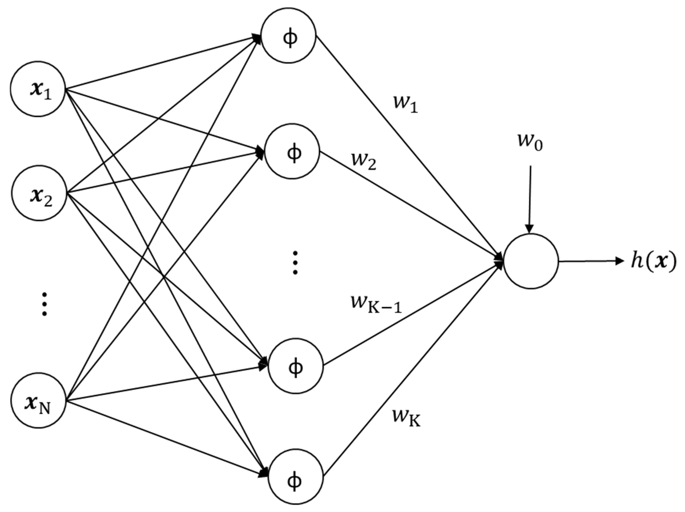
5.1. Numerical Simulations and Performance Comparison
Numerical experiments were carried out to test the performance of the proposed PSO–RBNN algorithm in terms of convergence, model complexity and generalization ability; convergence and model complexity were gauged using MSE on the training set (Equation (3)), and a suitable test set was used to assess generalization ability. A MATLAB R2020b code for the PSO–RBNN algorithm was developed and tested on different types of analytical test problems involving real-valued functions [
24]. The test functions were chosen to cover problems with varying dimensions and complexity. The functional forms of the test problems are given as follows:
One-dimensional Function
where
.
Booth Function
where
.
Six–Hump Camel Back Function
where
.
Hartmann 3 Function
where
.
, and
b and
d are given by
Hartmann 6 Function
where
.
, and
b and
d are given by
The training, validation and test data sets were generated using the Latin hypercube sampling (LHS) technique [
25,
26]. LHS is a widely used design-of-experiment (DOE) procedure used by many researchers, owing to its better space-filling property, sample flexibility and small sample sizes. In the present study,
lhsdesign (MATLAB built-in function for LHS) was used to generate the sample points with the criterion ‘maximin’ (maximize the minimum distance between points). It is an iterative method that generates LHS samples at random and chooses the best one based on the criterion ‘
maximin’. To construct the experimental design (sample), the number of sample points is specified by the user.
Table 1 presents the details of the test functions and the corresponding data sets used in the present study. The numerical experiments were performed using a computer with an Intel Core i7 processor (assembled, Seoul, Republic of Korea) with four CPUs, 16 GB RAM, and a clock speed of 3.40 GHz in serial processing mode. Furthermore, a direct comparison of the PSO–RBNN algorithm with OLS learning (a well-known learning algorithm for RBF NN modeling) proposed by Chen et al. [
12] was conducted. For both methods, the network parameters, including the number and locations of neurons, were determined using the training dataset, while the optimal model selection with respect to the spread constant
was performed using the validation dataset. This validation-based selection prevents the network from overfitting the training data and improves the generalization performance of the network. Finally, the predictive performance of each model was then assessed using an independent test dataset.
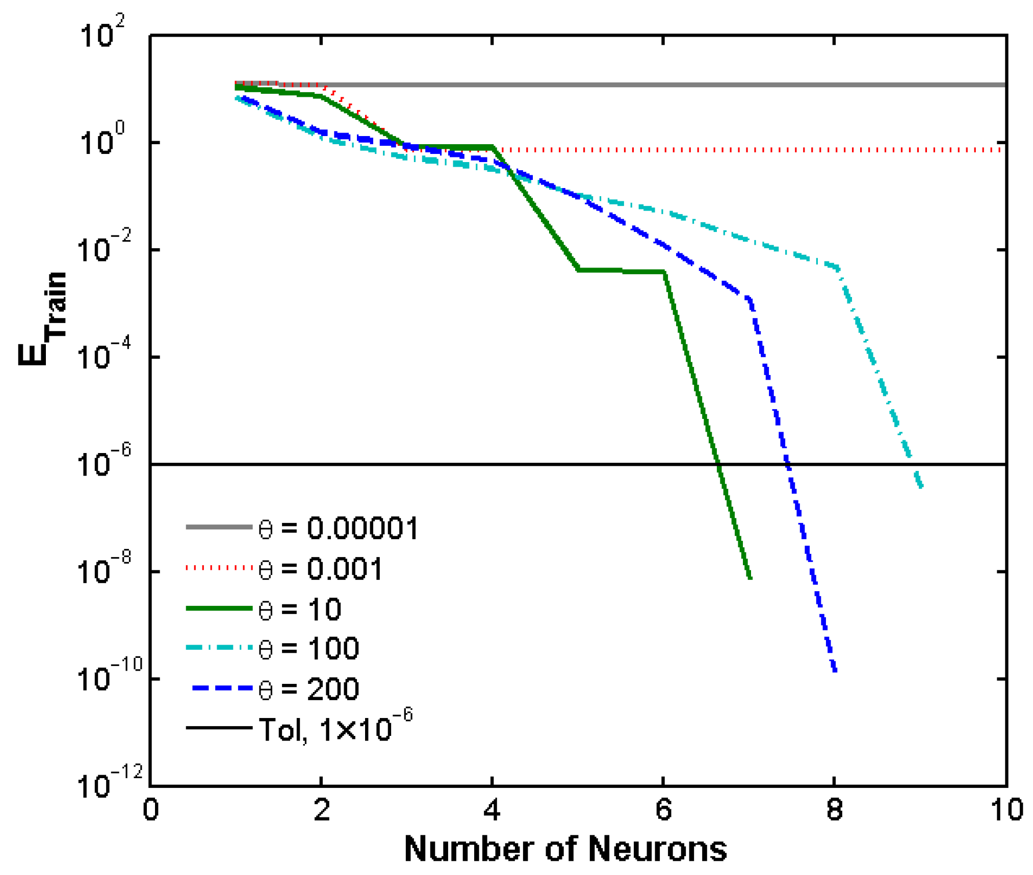
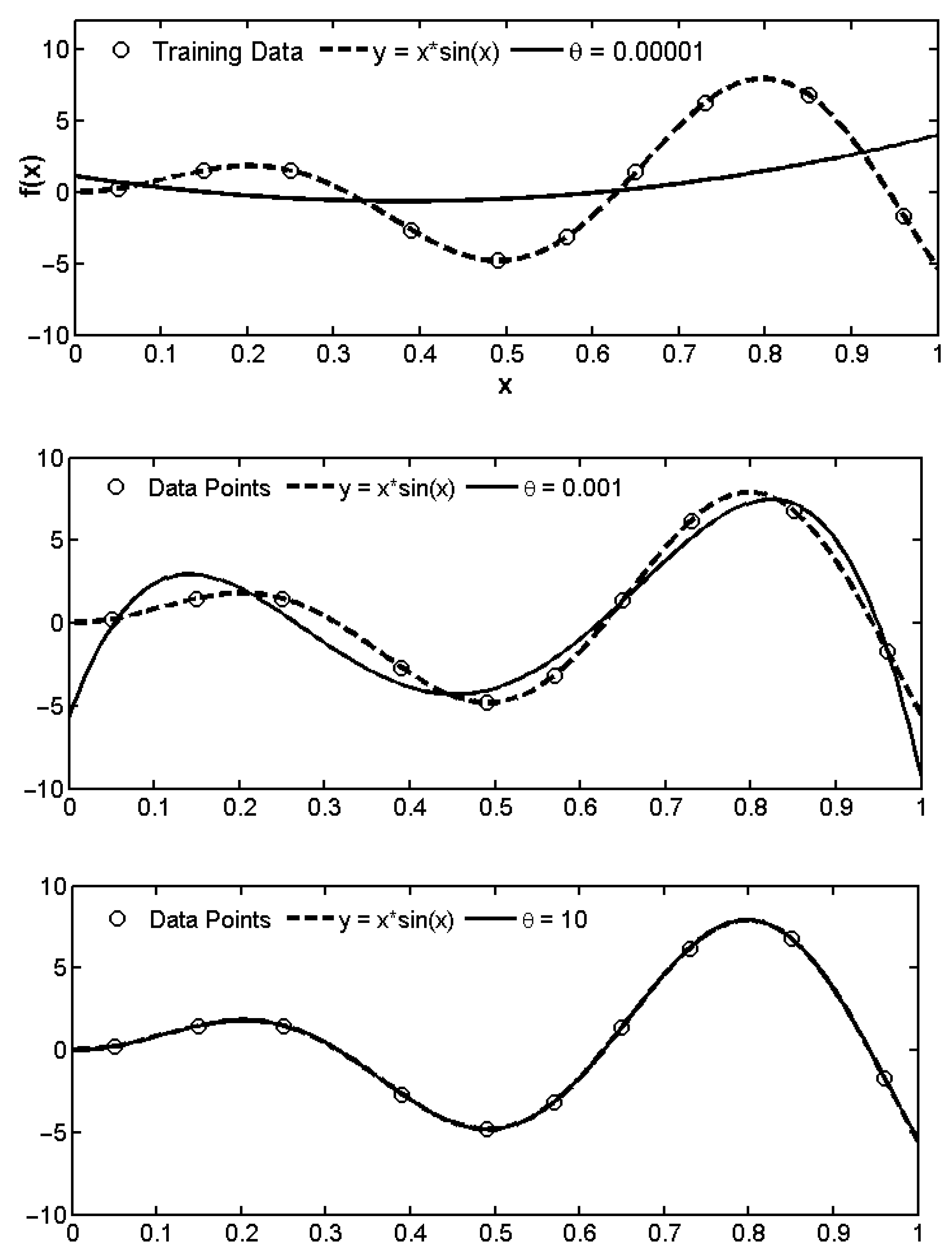
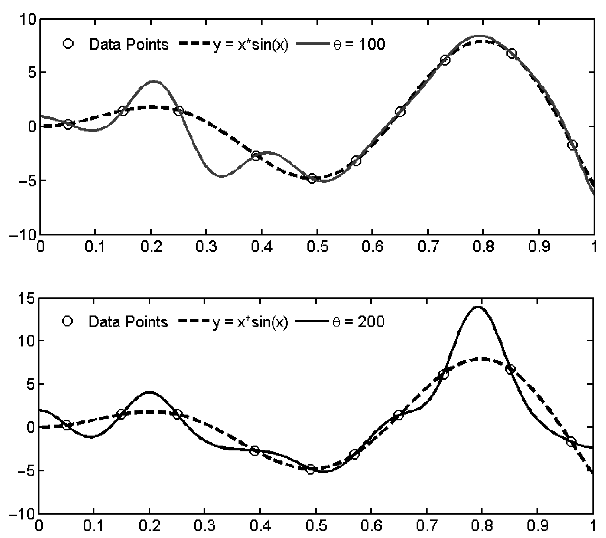
Figure 2 shows the evolution of training error with the number of neurons for a 1D function at different values of the spread constant, while the corresponding function approximations are shown in
Figure 3. This exercise was conducted to illustrate under- and over-fitting behavior associated with the choice of spread constant using the PSO–RBNN algorithm. For small values of the spread constant (
= 0.00001 and 0.001), underfitting will occur due to the large overlapping of the neurons, which leads to an ill-conditioned design matrix,
X in Equation (4). In such cases, the SVD uses low-rank approximation for
X to compute the linear weights, resulting in smoother approximation and reduced model flexibility.
As can be seen from
Figure 2, the network performs poorly on training data and is not able to reach the desired error goal. In contrast, for higher values of spread constant (
= 100 and 200), overfitting becomes a serious issue (the network performs very well on the training set but exhibits poor generalization ability). The neuron output is limited to a narrow range and dies out very quickly. At the optimal spread constant (
= 10), the overlap is within a certain level, resulting in sufficiently accurate approximation. Therefore, although the PSO–RBNN algorithm selects the centers from the input domain using optimization of the mean-squared error,
, the choice of spread constant has a significant influence on the solution. Consequently, model validation strategies, viz., validation set or cross-validation, are required for model selection as in other existing learning algorithms.
Table 2 lists the neuron centers and training error as both algorithms proceed towards convergence for the 1D function. As mentioned earlier, the optimum spread constant was found using a validation set for both the methods. The OLS–RBNN method selects the neuron centers directly from the training data, whereas the PSO–RBNN searches the input space to determine the optimum centers. As a result, the PSO–RBNN exhibits faster convergence and requires less neurons, as depicted in
Table 2.
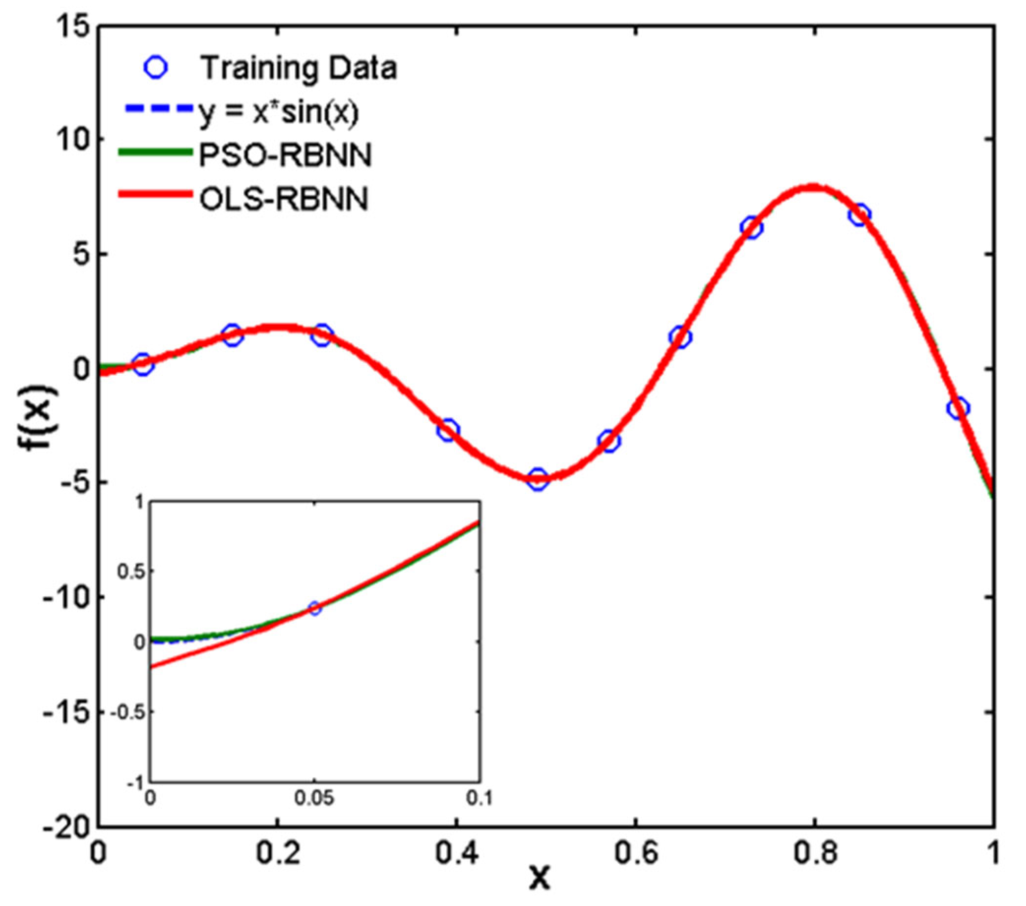
Figure 4 shows a comparison of the prediction accuracy between neural networks trained using the PSO–RBNN and OLS–RBNN algorithms.
The model performance with both the learning algorithms was found to be good, but the PSO–RBNN showed a slightly better prediction accuracy compared to the OLS–RBNN near the lower bound on the input variable, as shown in
Figure 4.
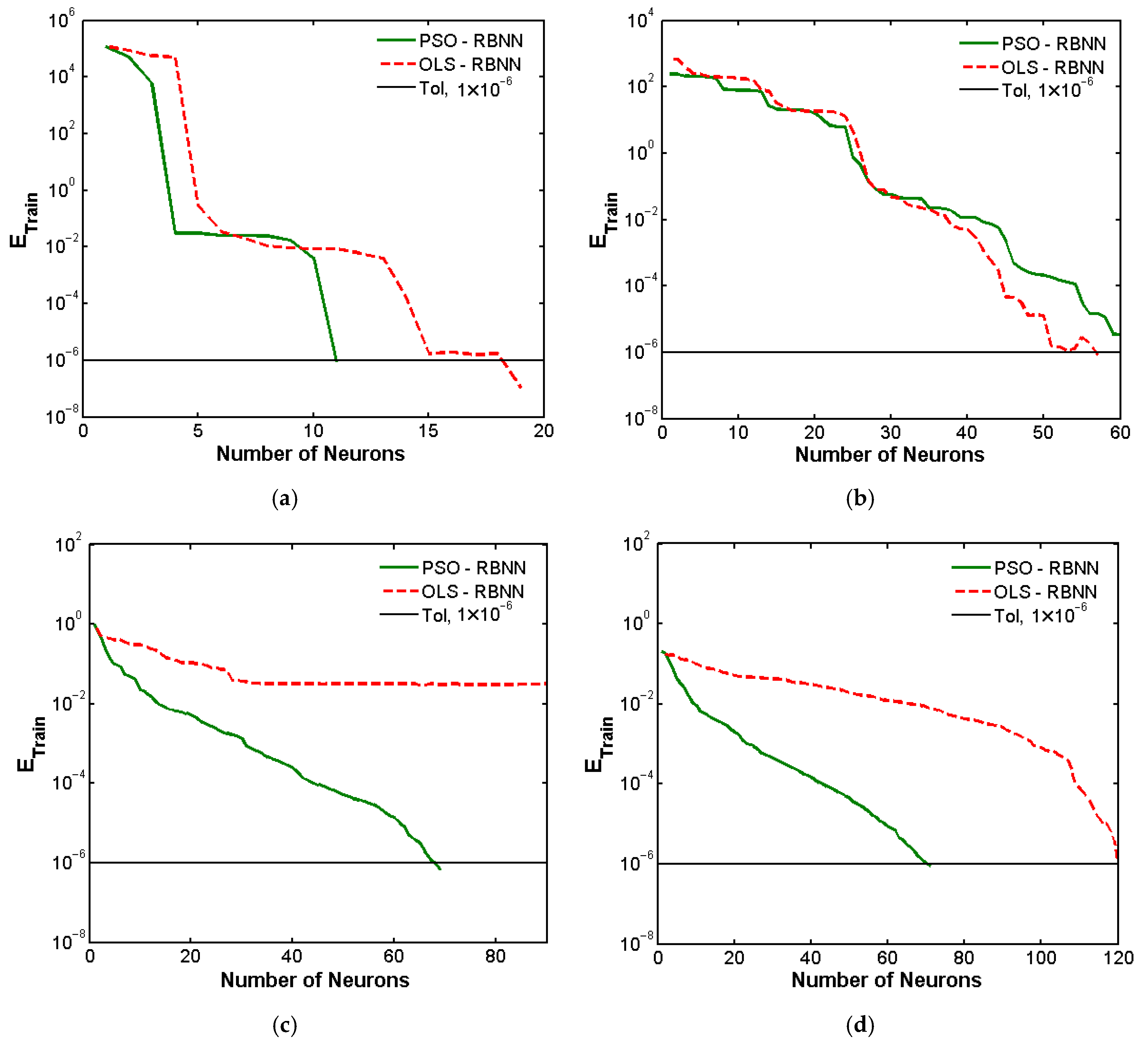
The evolution of training error with number of neurons—added to the network in a sequential manner—for the PSO–RBNN algorithm is shown in
Figure 5 and compared with the OLS method. The PSO–RBNN algorithm was simulated 20 times using the data sets for the test problems, and the best result, based on the validation and test data, was used for comparison. For most of the selected test problems, the PSO–RBNN algorithm outperforms the OLS–RBNN, except for the six-hump camel back function where it is slightly worse than the OLS method. In fact, the PSO–RBNN outperforms the OLS–RBNN right from the selection of the first neuron center, highlighting the efficacy of the PSO–based search strategy proposed in the present work. For Booth, Hartmann 3 and Hartmann 6 functions, a faster convergence behavior is observed for the PSO–RBF NN algorithm compared to the OLS–RBNN and significantly lower number of neurons is also required. For Hartmann 3 function, the OLS method fails to reach the specified error goal on the training set with a sufficiently large discrepancy whereas the PSO–RBF NN attains fast convergence as shown in
Figure 5c. The decreases in the number of neurons selected by the PSO–RBNN algorithm are found to be 36.84%, 22.21% and 41.67% for the Booth, Hartmann 3 and Hartmann 6 functions, respectively, compared with the OLS–RBNN algorithm.
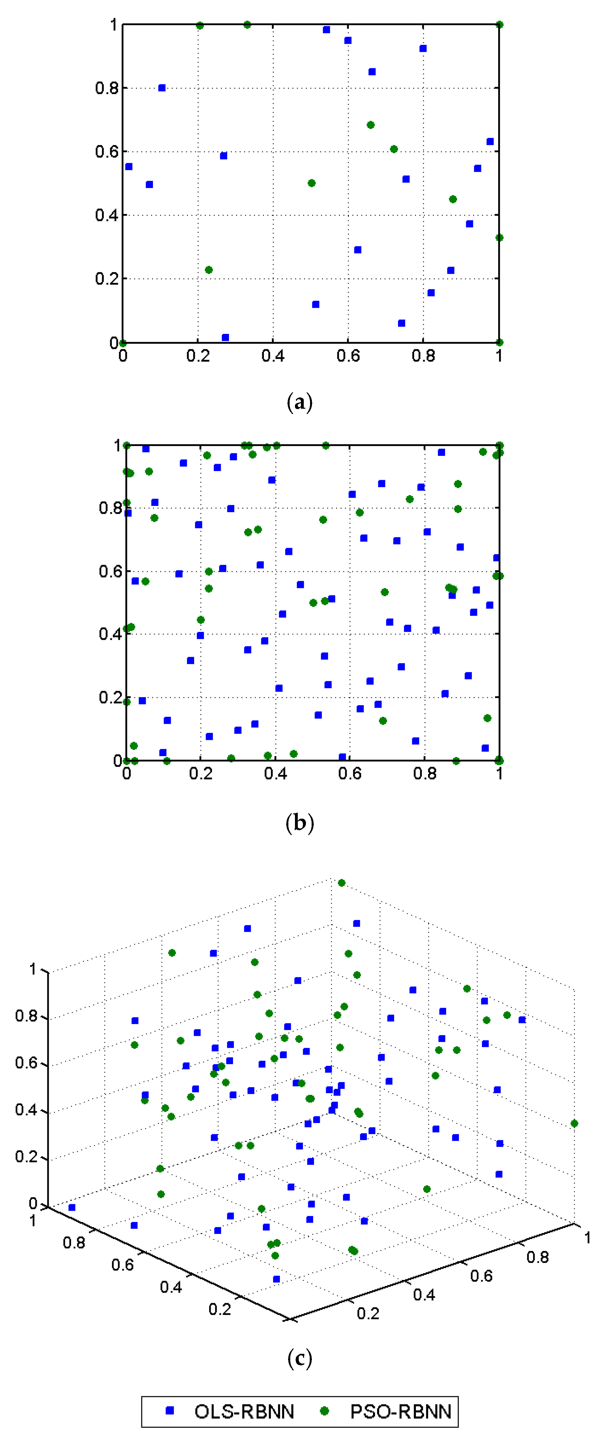
Figure 6 shows the distribution of neuron centers in the input domain obtained using the PSO– and OLS–RBNN algorithms for the optimal network structure. The neurons centers were obtained from the training data for the OLS method, whereas PSO was used to scan the entire space of the input variables to select the centers, as shown in
Figure 6; the neurons centers were not from the training points but selected randomly from the input domain based on the proposed PSO–RBNN algorithm. Localized clusters of neuron centers can be seen, which can be attributed to the fact that more centers are required in the regions where the variation in the objective function,
given by Equation (3), is expected to be large.
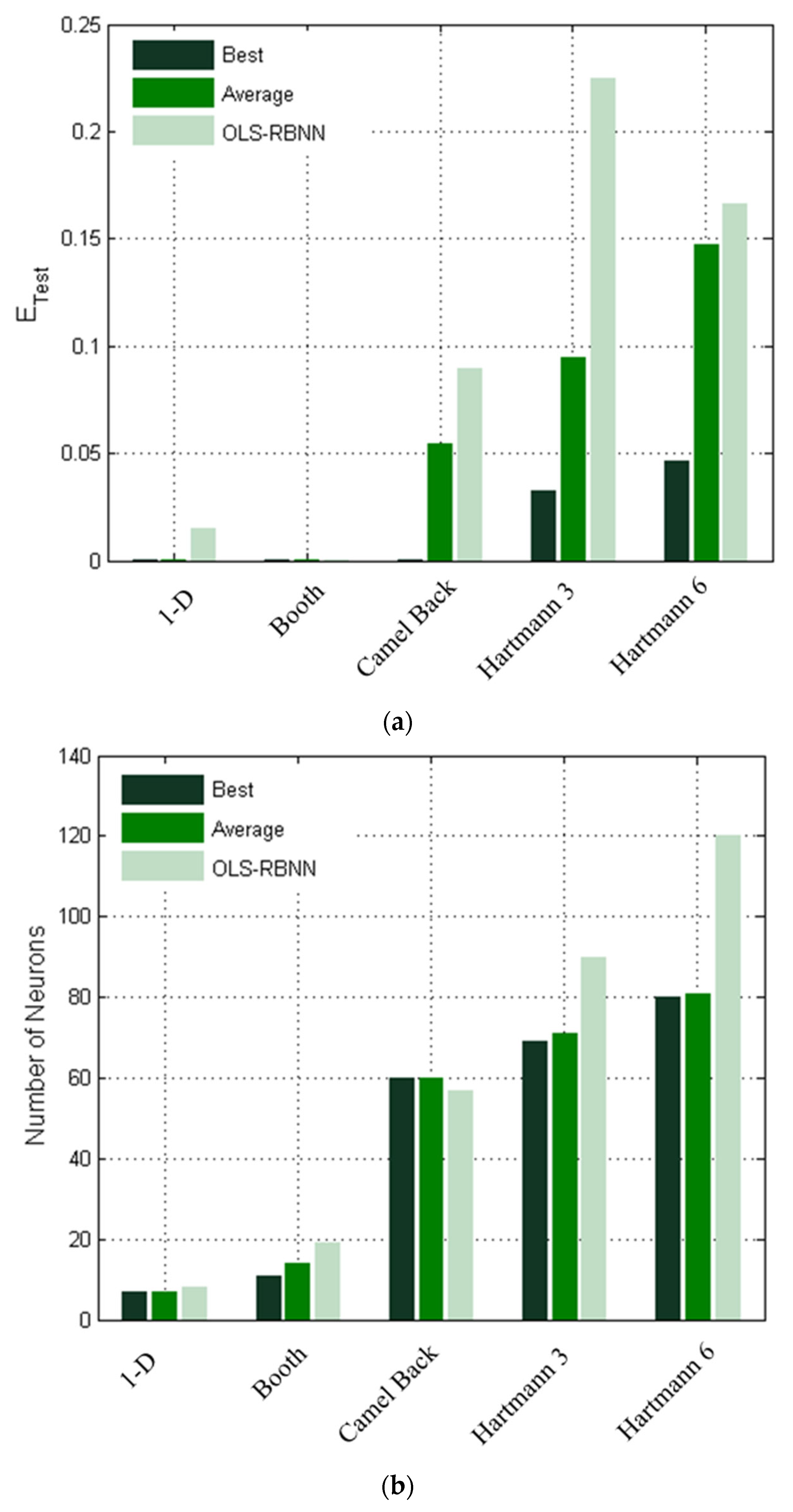
Figure 7 presents the mean-squared error on the test set,
, and the total number of selected neurons for the PSO–RBNN and OLS–RBNN algorithms. A comparison of the test error indicates superior generalization ability of the network trained by the PSO–RBNN algorithm, both in terms of the best outcome as well as the overall average across multiple trials as shown in
Figure 7a for all test problems. Interestingly, the best test error for the six-hump camel back function from the PSO–RBNN is found to be considerably lower than the OLS algorithm. Consequently, a slightly worse performance in the training is offset by a remarkable increase in the generalization ability of the network, which is important in the context of learning because the generalization error is the bottom line, not the training error. The training convergence curve shown in
Figure 5a corresponds to the trial yielding the minimum test error, since faster convergence was observed in some runs to coincide with poorer generalization. Furthermore, the PSO-RBNN requires a significantly lower number of neurons in comparison with the OLS–RBNN to develop the optimal network structure for all tested problems, except for the six-hump camel back function as shown in
Figure 7b. Thus, the PSO–RBF NN shows the best overall performance, namely learning and generalization, compared to the OLS method. Also, the PSO–RBNN algorithm tends to produce simpler models with a smaller number of parameters (number of neuron centers and weights in the linear layer).
As mentioned earlier, the PSO–RBNN algorithm was run 20 times using the data sets for the test problems, and therefore, the mean and standard deviations were computed. The training and test errors, together with the number of neurons, are summarized in
Table 3. The standard deviation for training error and number of neurons is found to be small, yielding a consistent network architecture, but different level variations in the test error are observed depending on the test problem; maximum variation is observed for the six-hump camel back function. Nevertheless, for the best model selection, one of the advantages of the variability in the generalization ability of the PSO–RBNN algorithm is that one can make a choice of a very good model from a candidate pool of well-performing models.
PSO has been used previously by different authors to develop RBNN architecture, and therefore, the predictive performance and convergence properties of the proposed PSO–RBNN algorithm are compared with two popular existing algorithms, PSO–NSFM by Alexandridis et al. [
18] and pRBF NN by Oh et al. [
17]. To compare with the PSO–NSFM algorithm, two test problems were selected as follows:
Friedman [
25]
where
and
is a Gaussian noise ~ N(0, 0.8).
Samad [
26]
where
and
is a Gaussian noise ~ N(0, 0.025).
For each case, the data were split randomly for training (50%), validation (25%) and testing (25%) subsets, following the procedure of Alexandridis et al. [
18].
Table 4 compares the root mean squared error (RMSE) for the validation and test sets between PSO–RBNN and PSO–NSFM, together with the corresponding number of hidden neurons. It can be observed that the proposed PSO–RBNN consistently achieves lower or comparable RMSE values relative to PSO–NSFM, while requiring a significantly smaller network size. This reduction in the number of neurons indicates improved parsimony without compromising predictive accuracy. The results confirm that the direct optimization of RBF centers using PSO, combined with least-squares weight estimation, provides strong generalization capability on chose nonlinear benchmark problems.
An additional study was conducted to examine the effect of training sample distribution and noise characteristics on the generalization performance of the PSO–RBNN algorithm. The results, averaged over 20 independent trials, are summarized in
Table 5 for two cases: noise-free data with noisy data generated from a specified Gaussian distribution. For both the Friedman [
27] and Samad [
28] datasets, the PSO–RBNN exhibits low RMSE values in noise-free cases, confirming its strong generalization ability. When noise is introduced, an expected increase in RMSE is observed; however, a reasonable and controlled adjustment in the number of neurons and generalization error was evident in both cases, reflecting the adaptive nature of the proposed learning strategy.
The robustness of the PSO–RBNN algorithm to noise was further investigated using different Gaussian noise distributions, as reported in
Table 6. Although the presence of noise leads to higher prediction errors, the overall increase in RMSE remains moderate, indicating stable learning behavior. Importantly, the network size does not increase excessively under noisy conditions, demonstrating that the proposed approach avoids overfitting and maintains a compact network structure even when the data are corrupted by stochastic disturbances. These results collectively highlight the robustness of PSO–RBNN with respect to variations in both noise level and training sample distribution, owing to its adaptive center selection and validation-based control of model complexity.
For comparison with the pRBF NN algorithm, two real-world datasets, (a) Automobiles miles per gallon (MPG), and (b) Boston housing, were used. Each dataset was randomly split into training (60%) and testing (40%) subsets, following the procedure of Oh et al. [
17].
Table 7 compares the root mean squared error (RMSE) values obtained on the training and test sets for the PSO–RBNN and pRBF NN. The PSO–RBF NN algorithm demonstrates superior generalization ability but requires more neurons compared to the pRBF NN approach. However, the overall computational effort for PSO–RBNN is significantly lower than pRBF NN, as the latter involves additional computation of polynomial coefficients.
Finally, a 1D function [
29] commonly used in different research works is used in the present study to compare the performance of the present PSO–RBF NN algorithm with the existing algorithms such as DFNN [
30], GA–RBF [
29] and SO–RBF [
19]. The function form is as follows:
The size of the training and test samples was set to 200, each obtained using LHS, and randomly distributed in the interval [0, 2].
Table 8 shows the detailed results of the comparison of different algorithms. The present PSO–RBF NN algorithm showed significant improvement in the generalization ability and required a lower number of neurons compared with the given existing algorithms.