Learning Dynamics from Data by Future-Informed Regression of Evolution

Abstract

The data-driven modeling of nonlinear dynamical systems using the Koopman operator has become a widely adopted framework for spectral analysis, prediction, and control. However, classical Koopman-based methods are typically restricted to observables defined on the system state at a single time instant, which limits their expressivity for systems exhibiting temporal correlations, memory effects, or multi-step interactions. In this work, we introduce a generalized linear mapping operator designed to establish the optimal linear relationship between two complex, trajectory-dependent observables defined over an extended state space that incorporates both past and future dynamics. By allowing heterogeneous input–output observable spaces, the proposed framework systematically captures temporal dependencies, coupled dynamics, and physically informed features, extending the applicability of Koopman-based data-driven modeling. Numerical experiments on benchmark systems, including the SIR epidemic model, a two-mass spring–damper system, and a forced harmonic oscillator, demonstrate improved reconstruction accuracy and spectral representation compared to standard approaches. In particular, the proposed method achieves relative reconstruction errors as low as $5.89\times {10}^{-5}$ for the SIR model and $8.96\times {10}^{-4}$ for the forced harmonic oscillator, representing improvements of several orders of magnitude over classical DMD and EDMD variants. These results confirm the robustness of the new framework in capturing complex nonlinear and transient dynamics.

1. Introduction

The analysis and prediction of complex nonlinear dynamical systems remains a central challenge across numerous scientific and engineering disciplines. Traditional approaches often rely on linearizations around equilibrium points or computationally intensive nonlinear simulation techniques. The Koopman operator framework [1,2] provides a powerful alternative, lifting nonlinear dynamics into an infinite-dimensional linear function space of observables. A renewed interest in Koopman analysis has emerged since the pioneering work of Mezić and collaborators [3,4,5], enabling spectral analysis and the prediction of nonlinear systems using data-driven approximations.

Dynamic Mode Decomposition (DMD) has become a prominent method for data-driven analysis, offering a linear approximation of the underlying dynamics in terms of spatial modes and associated eigenvalues [6,7,8]. DMD and its extensions have found applications in neuroscience [9], epidemiology [10], video processing [11], cavity flows [6], financial trading [12,13], and robotics [14]. Comprehensive reviews of the DMD literature are provided in [8,15,16], and recent modifications are discussed in [17,18,19,20,21].

Despite their successes, standard DMD methods are limited to linear observables directly associated with the state variables. This can lead to insufficient performance in strongly nonlinear systems. To address this, several extensions have been developed, including Extended Dynamic Mode Decomposition (EDMD) [22], Hankel (delay-embedding) DMD [23,24,25], DMD with Control (DMDc) [26,27,28], Optimized or Robust DMD [29], and Forward–Backward DMD (fbDMD) [30]. EDMD, in particular, generalizes DMD by projecting the dynamics onto a user-defined dictionary of nonlinear observables, enabling approximation of the Koopman operator for a wide range of nonlinear systems, including fluid flows, mechanical oscillators, and reaction–diffusion models [31]. Extensions aimed at enhancing expressivity and numerical stability include multi-resolution DMD [8], sparsity-promoting DMD [19], and kernel-based approaches [32,33,34,35,36,37].

The shift toward continuous-time data-driven modeling has gained significant momentum in recent years, reflecting the need for frameworks that align naturally with physical laws. Recent developments include data-driven continuous-time Hammerstein modeling addressing missing data [38], iterative learning control (ILC) for continuous-time systems [39], and continuous-time surrogate models for dynamic optimization [40]. These advances highlight the growing relevance of continuous-time operator representations and motivate the introduction of the proposed framework, which further enhances numerical stability, reconstruction accuracy, and spectral fidelity.

A common limitation of standard DMD and EDMD formulations is the restriction of observables to functions of the system state at a single time instant. This constraint can reduce the expressive power of the approximation, particularly in systems exhibiting temporal correlations, memory effects, or multi-step interactions. Time-delay embedding techniques, based on the Takens embedding theorem [41] and integrated with DMD or EDMD [24,42], allow observables to depend on sequences of past states, improving spectral approximations in quasi-periodic or chaotic systems. For a thorough review, see [42,43,44].

In this work, we introduce the Future-Informed Regression Evolution (FIRE) framework, a generalized operator-theoretic approach that extends the Koopman operator to map between heterogeneous spaces of multi-state observables. Unlike traditional EDMD or Hankel-DMD approaches [22,23,24], FIRE allows each observable to depend on a sequence of past, current, and future states, forming an extended information state. This enables the operator to capture temporal correlations, nonlinear cross-terms, derivatives, or other physically informed features that may differ between input and target spaces. By formalizing the input–output relationship via a general mapping $\pi :\mathcal{X}\to \mathcal{Y}$, FIRE generalizes the classical Koopman framework and systematically handles partial or scalar measurements while preserving spectral properties.

We demonstrate the effectiveness of FIRE on benchmark systems, including the SIR epidemic model, a two-mass spring–damper system, and the forced harmonic oscillator. The numerical results indicate improved reconstruction accuracy and spectral representation compared to standard DMD and EDMD variants.

The main contributions of this study are summarized as follows:

1.

We introduce a rigorous operator-theoretic formulation of the generalized transfer operator $\mathcal{G}$, capturing the evolution of extended observables across heterogeneous spaces while preserving spectral properties under mild assumptions.

2.

We provide both continuous-time and discrete-time numerical realizations via finite-dimensional Galerkin approximations, connecting FIRE to EDMD and Hankel-DMD while highlighting its distinct advantages.

3.

Through numerical experiments on benchmark systems, we demonstrate that FIRE achieves superior reconstruction accuracy and robust spectral representation, even from partial or scalar observations.

The remainder of this paper is organized as follows. Section 2 reviews Koopman operator preliminaries. Section 3 presents the mathematical formulation of the FIRE framework, followed by the data-driven approximation of the generalized operator in Section 4. Section 5 presents the numerical experiments, and Section 6 concludes the paper.

2. Preliminary Theory

This section reviews the classical Koopman operator framework, discusses its finite-dimensional approximations via DMD and EDMD, and motivates the extension of the observable space to accommodate trajectory-dependent representations, which forms the basis for the generalized operator introduced in the subsequent section.

2.1. The Classical Koopman Framework

The Koopman operator provides a linear, operator-theoretic framework for the analysis of nonlinear dynamical systems by lifting the state evolution into a space of observables. This perspective enables the study of nonlinear dynamics using spectral methods traditionally associated with linear systems.

Let $(\mathcal{M},\mu )$ denote the phase space equipped with an invariant measure $\mu$. Consider a discrete-time nonlinear dynamical system governed by the following map:

$${\mathit{x}}_{k+1}=F\left({\mathit{x}}_k\right),{\mathit{x}}_k\in \mathcal{M}\subseteq {\mathbb{R}}^n.$$

(1)

Let $\mathcal{F}$ be a linear space of complex-valued observables $g:\mathcal{M}\to \mathbb{C}$ that is closed under composition with F, i.e.,

$$g\circ F\in \mathcal{F}\mathrm{for}\mathrm{all}g\in \mathcal{F},$$

where ∘ denotes functional composition. A common choice is $\mathcal{F}=L^2(\mathcal{M},\mu )$.

The Koopman operator $\mathcal{K}:\mathcal{F}\to \mathcal{F}$ associated with the dynamics (1) is defined by

$$\left(\mathcal{K}g\right)\left(\mathit{x}\right)=g\left(F\right(\mathit{x}\left)\right).$$

(2)

Unlike the nonlinear map F, which acts on the state space $\mathcal{M}$, the Koopman operator acts on observables. Although $\mathcal{K}$ is generally infinite-dimensional—even when F is finite-dimensional—it is linear, even for strongly nonlinear systems. Specifically, for any $g_1,g_2\in \mathcal{F}$ and scalars $c_1,c_2\in \mathbb{C}$,

$$\mathcal{K}(c_1{g}_1+c_2{g}_2)=c_1\mathcal{K}{g}_1+c_2\mathcal{K}{g}_2.$$

(3)

A function $\varphi \in \mathcal{F}$ is called a Koopman eigenfunction associated with the eigenvalue $\lambda \in \mathbb{C}$ if

$$\mathcal{K}\varphi =\lambda \varphi .$$

(4)

Combining (2) and (4), the eigenfunctions satisfy

$$\varphi \left(F\right(\mathit{x}\left)\right)=\lambda \varphi \left(\mathit{x}\right),$$

(5)

which implies that Koopman eigenfunctions evolve linearly along trajectories of the nonlinear system. This property forms the foundation for Koopman spectral analysis.

Suppose that the observable $g\in \mathcal{F}$ lies in the span of Koopman eigenfunctions ${\left\{{\varphi }_j\right\}}_{j=1}^{\infty }$, allowing the expansion

$$g\left(\mathit{x}\right)=\sum _{j=1}^{\infty }{v}_j{\varphi }_j\left(\mathit{x}\right),$$

(6)

where the coefficients $v_j\in \mathbb{C}$ are referred to as Koopman modes. For a vector-valued observable $\mathit{g}:\mathcal{M}\to {\mathbb{C}}^n$,

$$\mathit{g}\left(\mathit{x}\right)={[g_1\left(\mathit{x}\right),\dots ,g_n\left(\mathit{x}\right)]}^T,$$

a similar expansion holds, as follows:

$$\mathit{g}\left(\mathit{x}\right)=\sum _{j=1}^{\infty }{\mathit{v}}_j{\varphi }_j\left(\mathit{x}\right),$$

(7)

where ${\mathit{v}}_j\in {\mathbb{C}}^n$ denote the Koopman modes associated with ${\varphi }_j$.

Applying the Koopman operator yields

$$\mathit{g}\left(F\left(\mathit{x}\right)\right)=\sum _{j=1}^{\infty }{\lambda }_j{\mathit{v}}_j{\varphi }_j\left(\mathit{x}\right),$$

(8)

and, by repeated application,

$$\mathit{g}\left(F^k\left(\mathit{x}\right)\right)=\sum _{j=1}^{\infty }{\lambda }_j^k{\mathit{v}}_j{\varphi }_j\left(\mathit{x}\right),$$

(9)

where $F^k$ denotes the k-fold composition of F. Each Koopman mode evolves independently with growth rate and oscillatory behavior determined by the corresponding eigenvalue ${\lambda }_j$.

The collection of triples ${\left\{({\lambda }_j,{\varphi }_j,{\mathit{v}}_j)\right\}}_{j=1}^{\infty }$ constitutes the Koopman mode decomposition, originally introduced by Mezić [3]. When the full state is observable (i.e., $g_i\left(\mathit{x}\right)=x_i$), the Koopman operator provides a complete linear representation of the nonlinear dynamics.

Despite its conceptual elegance, the classical Koopman framework restricts observables to functions of the instantaneous system state. This limitation motivates the development of generalized operator constructions capable of incorporating trajectory-dependent and multi-state information, which form the basis of the FIRE framework introduced in the following sections.

2.2. Dynamic Mode Decomposition and Extended Dynamic Mode Decomposition

The Koopman operator is, in general, infinite-dimensional, which renders its direct numerical computation infeasible. Practical implementations therefore rely on finite-dimensional approximations obtained by restricting the operator to suitably chosen subspaces of observables. A variety of data-driven methods have been proposed to construct such approximations, among which Dynamic Mode Decomposition (DMD) and its generalization, Extended Dynamic Mode Decomposition (EDMD), are the most widely used.

Dynamic Mode Decomposition provides a numerical approximation of the Koopman operator based on linear observables of the system state. While DMD has proven effective in many applications, its reliance on linear measurements limits its ability to capture strongly nonlinear dynamics. Extended Dynamic Mode Decomposition was introduced to address this limitation by approximating the Koopman operator in a richer, user-defined space of nonlinear observables.

In EDMD, the infinite-dimensional Koopman operator $\mathcal{K}$ is approximated by its projection onto a finite-dimensional subspace spanned by a prescribed dictionary of observables. Let

$$\mathcal{D}=\{{\psi }_1,\dots ,{\psi }_N\},$$

where each ${\psi }_i:\mathcal{M}\to \mathbb{C}$ belongs to the observable space $\mathcal{F}$. We denote by

$${\mathcal{F}}_{\mathcal{D}}=\mathrm{span}\{{\psi }_1,\dots ,{\psi }_N\}\subseteq \mathcal{F}$$

the finite-dimensional subspace generated by the dictionary. The objective of EDMD is to construct a matrix $K\in {\mathbb{C}}^{N\times N}$ that approximates the action of the Koopman operator restricted to ${\mathcal{F}}_{\mathcal{D}}$.

Assume that snapshot pairs ${\left\{({\mathit{x}}_k,{\mathit{y}}_k)\right\}}_{k=1}^M$ are collected from the dynamical system, where

$${\mathit{y}}_k=F\left({\mathit{x}}_k\right),{\mathit{x}}_k,{\mathit{y}}_k\in \mathcal{M}.$$

Define the feature map associated with the dictionary as

$$\mathit{\psi }\left(\mathit{x}\right)=\left[\begin{array}{c}{\psi }_1\left(\mathit{x}\right)\\ ⋮\\ {\psi }_N\left(\mathit{x}\right)\end{array}\right].$$

(10)

Using this feature map, EDMD constructs the data matrices

$$X=[\mathit{\psi }\left({\mathit{x}}_1\right)\cdots \mathit{\psi }\left({\mathit{x}}_M\right)],Y=[\mathit{\psi }\left({\mathit{y}}_1\right)\cdots \mathit{\psi }\left({\mathit{y}}_M\right)],$$

(11)

where $X,Y\in {\mathbb{C}}^{N\times M}$.

The finite-dimensional approximation of the Koopman operator is obtained by solving the least squares problem

$$\underset{K\in {\mathbb{C}}^{N\times N}}{min}{\parallel Y-KX\parallel }_F^2,$$

(12)

which admits the solution

$$K=Y{X}^{†},$$

(13)

where $X^{†}$ denotes the Moore–Penrose pseudoinverse of X. The resulting matrix K represents the projection of the Koopman operator onto the subspace ${\mathcal{F}}_{\mathcal{D}}$ spanned by the chosen dictionary. Its spectral decomposition provides finite-dimensional approximations of Koopman eigenvalues, eigenfunctions, and modes, enabling the reconstruction and prediction of system dynamics.

The quality of the EDMD approximation critically depends on the choice of dictionary. If ${\mathcal{F}}_{\mathcal{D}}$ is invariant under the action of the Koopman operator, the approximation is exact on this subspace and the residual in (12) vanishes. In practice, however, Koopman-invariant subspaces are rarely known a priori. When the dictionary does not span such a subspace, the projected operator may introduce spurious eigenvalues and eigenfunctions, and important dynamical features may be lost. In the limit of infinite data, the EDMD matrix converges to the Koopman operator projected onto ${\mathcal{F}}_{\mathcal{D}}$, but this projection error persists unless the dictionary is sufficiently expressive.

Dynamic Mode Decomposition arises as a special case of EDMD when the dictionary consists solely of the identity observable,

$$\mathit{\psi }\left(\mathit{x}\right)=\mathit{x}.$$

(14)

In this case, EDMD reduces to a linear approximation of the Koopman operator acting directly on the state space, highlighting DMD as a particular instance within the broader EDMD framework.

3. Generalized Sequence-Based Evolution Operator

The Koopman operator framework provides a powerful tool for representing nonlinear dynamics through the linear evolution of observables. Traditional formulations, however, typically consider observables defined on a single state at a fixed time, limiting their applicability to systems with temporal correlations, memory effects, or heterogeneous representations across time. To address these limitations, we introduce a generalized sequence-based evolution operator, designed to establish a linear mapping between observables defined over sequences of system states. By constructing the operator on spatio-temporal windows of feature vectors rather than the state space itself, this approach enables the incorporation of past, present, and future information in a unified framework. The operator preserves linearity in the space of observables and induces a structured evolution that can be interpreted as Markovian in the expanded feature space, providing a principled link between high-fidelity trajectories and reduced-order or aggregated representations.

3.1. Generalized Sequence-Based Operator

We now formalize the central concept of this work: a generalized evolution operator acting on multi-state observables.

Consider a discrete-time dynamical system on a state manifold $\mathcal{M}\subset {\mathbb{R}}^n$, governed by the map

$${\mathit{z}}_{k+1}=F\left({\mathit{z}}_k\right),{\mathit{z}}_k\in \mathcal{M}.$$

(15)

Definition 1

(Extended State). Let ${\left\{{\mathit{z}}_k\right\}}_{k\in \mathbb{Z}}\subset {\mathbb{R}}^n$ be a discrete-time process. For fixed non-negative integers $d,s\in {\mathbb{N}}_0$ (memory depth and anticipation depth), the extended state at time k is defined as follows:

$${\tilde{\mathit{z}}}_k=\left[\begin{array}{c}{\mathit{z}}_{k-d}\\ ⋮\\ {\mathit{z}}_k\\ ⋮\\ {\mathit{z}}_{k+s}\end{array}\right]\in {\mathbb{R}}^{(d+s+1)n}.$$

(16)

The extended state aggregates a finite window of past, current, and (optionally) future states into a single vector. The corresponding extended state space is defined as a Cartesian product, as follows:

$${\mathcal{M}}^q=\underset{q\mathrm{copies}}{\underbrace{\mathcal{M}\times \cdots \times \mathcal{M}}}\subset {\mathbb{R}}^{qn}.$$

(17)

Definition 2

(Multi-State Observable). A multi-state observable is a measurable function,

$$g:{\mathcal{M}}^q\to \mathbb{C},$$

for a fixed integer $q\ge 0$.

The space of all such observables, denoted $\mathcal{F}\left({\mathcal{M}}^q\right)$, forms the feature space for extended observables. Lifting the analysis to $\mathcal{F}\left({\mathcal{M}}^q\right)$ enables the incorporation of bidirectional temporal dependence and trajectory-based information.

To formalize input–output relationships across extended states, we introduce two distinct observation spaces:

$$\mathcal{X}={\mathcal{M}}^{d+s+1},\mathcal{Y}={\mathcal{M}}^{r+l+1},$$

(18)

with associated observable spaces $\mathcal{F}\left(\mathcal{X}\right)$ and $\mathcal{F}\left(\mathcal{Y}\right)$.

Definition 3

(Generalized Operator $\mathcal{G}$). Let $\mathcal{X}$ and $\mathcal{Y}$ be two state spaces as in (18), and let $\pi :\mathcal{X}\to \mathcal{Y}$ be a measurable map encoding temporal alignment. The generalized operator

$$\mathcal{G}:\mathcal{F}\left(\mathcal{Y}\right)\to \mathcal{F}\left(\mathcal{X}\right)$$

is defined by

$$\left(\mathcal{G}g\right)\left(\mathit{x}\right):=h\left(\mathit{x}\right),$$

(19)

where $h\left(\mathit{x}\right)=g\left(\pi \right(\mathit{x}\left)\right)$ with $\mathit{x}\in \mathcal{X}$ and $g\in \mathcal{F}\left(\mathcal{Y}\right)$.

In other words, $\mathcal{G}$ maps a target observable g defined on $\mathcal{Y}$ to a corresponding observable h on $\mathcal{X}$ through composition with $\pi$, establishing a linear correspondence between extended-state features:

$$\left(\mathcal{G}g\right)\left(\mathit{x}\right)=g\left(\mathit{y}\right),\mathrm{where}\mathit{y}=\pi \left(\mathit{x}\right).$$

(20)

This construction allows multi-state observables to depend on sequences of past, current, and future states while preserving linearity in the lifted feature space.

Unlike traditional transfer operators, which describe the temporal evolution of observables within a single state space, the operator $\mathcal{G}$ encodes the informational transfer between distinct extended-state representations of the same system. Equation (19) generalizes the classical Koopman action

$$\left(\mathcal{K}g\right)\left({\mathit{x}}_k\right)=g\left({\mathit{x}}_{k+1}\right)$$

by allowing the evolved observable to depend on a local sequence of feature vectors rather than a single state. In this sense, $\mathcal{G}$ extends the classical Koopman composition rule to encompass non-Markovian and sequence-dependent transformations.

The operator $\mathcal{G}$ can be interpreted as a natural generalization of the Koopman operator: it reduces to the classical Koopman operator $\mathcal{K}$ when the map $\pi$ coincides with the graph of the system evolution F, the target space $\mathcal{Y}$ is isomorphic to the input space $\mathcal{X}$, and $\mathcal{X}\equiv \mathcal{Y}\equiv \mathcal{M}$. Under these conditions, $\mathcal{G}$ recovers the standard Koopman action on single-time observables.

The incorporation of future states in the extended space $\mathcal{X}$ may appear related to backward-time or forward–backward DMD (fbDMD) formulations. However, the proposed framework differs fundamentally in both purpose and interpretation. Backward-time and fbDMD methods introduce reverse-time operators or symmetric constraints to improve numerical stability of Koopman eigenvalue estimates. In contrast, the anticipation depth in the present work is introduced at the level of state space construction, defining an augmented forward-time dynamical system with induced shift dynamics.

The generalized operator $\mathcal{G}$ does not approximate backward evolution, nor does it combine forward and backward operators. Instead, it acts as an intertwining map between Koopman operators on different state spaces, enabling spectral transfer under a semiconjugacy condition. As a result, future states are treated as components of the lifted state rather than as targets of inverse-time dynamics. This distinction allows the proposed framework to remain valid even for non-invertible or dissipative systems, where backward-time Koopman operators are not well-defined.

On future-informed versus causal constructions. Although the proposed framework allows for the construction of extended information states that may include both past and future measurements relative to a reference time index, this choice introduces a non-causal element when interpreted from a real-time prediction perspective. It is therefore important to distinguish between two different application regimes. In the first regime, during the offline analysis, such as system identification, spectral decomposition, or operator inference from archived datasets, access to future samples is available, and two-sided temporal windows are admissible. Including future measurements improves numerical conditioning and derivative estimation accuracy, particularly in continuous-time formulations, and leads to more faithful approximations of the infinitesimal generator. In the second regime, the online prediction or forecasting, where the future measurements are not available at inference time, once the operator and modal decomposition are learned, the learned Koopman modes evolve autonomously according to their eigenvalues, and only the current modal coordinates are propagated forward in time.

Moreover, the framework readily simplifies to a purely causal formulation by setting the anticipation depth to zero, reducing the method to a delay coordinate embedding based solely on past and present states. As such, the framework is applicable both in offline system identification and in online prediction scenarios where future data is unavailable.

In this work, the focus is on the offline analysis regime, where the goal is accurate operator identification and spectral characterization rather than real-time forecasting.

3.2. Theoretical Properties of the Generalized Operator $\mathcal{G}$

The operator $\mathcal{G}$ inherits linearity directly from the structure of the observable spaces. Specifically, since $\mathcal{F}\left(\mathcal{X}\right)$ is a vector space with pointwise addition and scalar multiplication, the action of $\mathcal{G}$ on linear combinations of observables preserves these operations. This property is formalized in the following result.

Lemma 1

(Linearity of $\mathcal{G}$). The generalized transfer operator $\mathcal{G}:\mathcal{F}\left(\mathcal{Y}\right)\to \mathcal{F}\left(\mathcal{X}\right)$ is linear.

Proof. 

Let $g_1, g_2\in \mathcal{F}\left(\mathcal{Y}\right)$ be two observables, and let $\alpha , \beta \in \mathbb{R}$ be arbitrary scalars. By definition of the generalized operator $\mathcal{G}$, for all $\mathit{x}\in \mathcal{X}$ we obtain

$$\left(\mathcal{G}{g}_i\right)\left(\mathit{x}\right)=g_i\left(\pi \left(\mathit{x}\right)\right),i=1,2,$$

where $\pi :\mathcal{X}\to \mathcal{Y}$ is the measurable map encoding temporal alignment.

Consider the linear combination $\alpha g_1+\beta g_2\in \mathcal{F}\left(\mathcal{Y}\right)$. Then, for all $\mathit{x}\in \mathcal{X}$,

$$\begin{array}{cc}\hfill \left(\mathcal{G}(\alpha g_1+\beta g_2)\right)\left(\mathit{x}\right)& =(\alpha g_1+\beta g_2)\left(\pi \left(\mathit{x}\right)\right)\hfill \\ & =\alpha g_1\left(\pi \left(\mathit{x}\right)\right)+\beta g_2\left(\pi \left(\mathit{x}\right)\right)\hfill \\ & =\alpha \left(\mathcal{G}{g}_1\right)\left(\mathit{x}\right)+\beta \left(\mathcal{G}{g}_2\right)\left(\mathit{x}\right).\hfill \end{array}$$

Since this holds for arbitrary $\mathit{x}\in \mathcal{X}$, we conclude that

$$\mathcal{G}(\alpha g_1+\beta g_2)=\alpha \mathcal{G}{g}_1+\beta \mathcal{G}{g}_2,$$

which proves that $\mathcal{G}$ is linear.    □

Theorem 1

(Dynamical Consistency via Lifting). Let $\mathcal{Y}$ be the physical state space with dynamics $F_{\mathcal{Y}}:\mathcal{Y}\to \mathcal{Y}$, and let $\mathcal{X}$ be an augmented (lifted) state space. Let $\pi :\mathcal{X}\to \mathcal{Y}$ be a measurable projection map. Assume there exists an induced dynamical map $F_{\mathcal{X}}:\mathcal{X}\to \mathcal{X}$ that is π-compatible, such that the following diagram commutes:

$$\pi \left(F_{\mathcal{X}}\left(\mathbf{x}\right)\right)=F_{\mathcal{Y}}\left(\pi \left(\mathit{x}\right)\right)\mathrm{for}\mathrm{all}\mathit{x}\in \mathcal{X}.$$

Let $\mathcal{G}:\mathcal{F}\left(\mathcal{Y}\right)\to \mathcal{F}\left(\mathcal{X}\right)$ be the generalized operator, according Definition 3, as follows:

$$\left(\mathcal{G}g\right)\left(\mathit{x}\right)=g\left(\pi \right(\mathit{x}\left)\right).$$

Then, the generalized operator preserves the temporal evolution of the observables:

$$\left(\mathcal{G}g\right)\left(F_{\mathcal{X}}\left(\mathit{x}\right)\right)=\left({\mathcal{K}}_{\mathcal{Y}}g\right)\left(\pi \left(\mathit{x}\right)\right)$$

(21)

where ${\mathcal{K}}_{\mathcal{Y}}$ is the Koopman operator on the physical space $\mathcal{Y}$.

Proof. 

Let $g\in \mathcal{F}\left(\mathcal{Y}\right)$ be an observable in the physical space, and let $h=\mathcal{G}g\in \mathcal{F}\left(\mathcal{X}\right)$ be its lifted counterpart defined by $\left(\mathcal{G}g\right)\left(\mathit{x}\right)=g\left(\pi \right(\mathit{x}\left)\right)$. We evaluate both sides of the identity (21) for an arbitrary point $\mathit{x}\in \mathcal{X}$.

By applying the definition of the generalized operator $\mathcal{G}$ to the point $F_{\mathcal{X}}\left(\mathit{x}\right)$, we obtain the following:

$$\left(\mathcal{G}g\right)\left(F_{\mathcal{X}}\left(\mathit{x}\right)\right)=g\left(\pi \left(F_{\mathcal{X}}\left(\mathit{x}\right)\right)\right).$$

(22)

Usingthe assumption of $\pi$-compatibility ($\pi \circ F_{\mathcal{X}}=F_{\mathcal{Y}}\circ \pi$), this expression becomes

$$g\left(\pi \left(F_{\mathcal{X}}\left(\mathit{x}\right)\right)\right)=g\left(F_{\mathcal{Y}}\left(\pi \left(\mathit{x}\right)\right)\right).$$

(23)

Now, consider the Koopman operator ${\mathcal{K}}_{\mathcal{Y}}$ acting on the physical space $\mathcal{Y}$, defined as follows:

$$\left({\mathcal{K}}_{\mathcal{Y}}g\right)\left(\mathit{y}\right)=g\left(F_{\mathcal{Y}}\left(\mathit{y}\right)\right).$$

Setting $\mathit{y}=\pi \left(\mathit{x}\right)$, we obtain

$$\left({\mathcal{K}}_{\mathcal{Y}}g\right)\left(\pi \left(\mathbf{x}\right)\right)=g\left(F_{\mathcal{Y}}\left(\pi \left(\mathbf{x}\right)\right)\right).$$

Combining the results from (22) and (23) yields

$$\left(\mathcal{G}g\right)\left(F_{\mathcal{X}}\left(\mathbf{x}\right)\right)=g\left(F_{\mathcal{Y}}\left(\pi \left(\mathbf{x}\right)\right)\right)=\left({\mathcal{K}}_{\mathcal{Y}}g\right)\left(\pi \left(\mathbf{x}\right)\right)\text{for} \text{all}\mathit{x}\in \mathcal{X},$$

which establishes the claimed dynamical consistency of lifted observables.    □

Remark 1.

Although the original dynamic (15) evolves on the state manifold $\mathcal{M}$, the delay-embedded space $\mathcal{X}$ carries induced shift dynamics $F_{\mathcal{X}}$, used to define the associated Koopman operatror ${\mathcal{K}}_{\mathcal{X}}$.

Remark 2.

In the context of the data-driven frameworks presented in this work, the spaces $\mathcal{X}$ and $\mathcal{Y}$ are typically delay-embedded manifolds (Hankel structures) constructed from the physical trajectory $\mathcal{M}$. In such cases, $F_{\mathcal{X}}$ and $F_{\mathcal{Y}}$ are naturally induced shift maps. Consequently, the projection map $\pi :\mathcal{X}\to \mathcal{Y}$, which acts as a truncation or window shift, automatically satisfies the semiconjugacy condition

$$\pi \circ F_{\mathcal{X}}=F_{\mathcal{Y}}\circ \pi .$$

(24)

This ensures that the generalized operator $\mathcal{G}$ is dynamically consistent with the underlying Koopman operator of the system, even under partial observability. Therefore, the dynamical consistency required in Theorem 1 holds automatically for delay coordinate constructions.

Rather than asserting generic validity, the following result identifies the precise structural condition under which the Koopman spectral information can be transferred between lifted and projected representations.

Theorem 2

(Commutation of Koopman Operators under Lifting). Let $\mathcal{X}$ and $\mathcal{Y}$ be state spaces equipped with induced discrete-time dynamical systems $F_{\mathcal{X}}$ and $F_{\mathcal{Y}}$, respectively, and let $\pi :\mathcal{X}\to \mathcal{Y}$ be a measurable map that induces a semiconjugacy between the dynamical systems $F_{\mathcal{X}}$ and $F_{\mathcal{Y}}$, i.e., satisfying (24). Let ${\mathcal{K}}_{\mathcal{X}}$ and ${\mathcal{K}}_{\mathcal{Y}}$ denote the Koopman operators associated with $F_{\mathcal{X}}$ and $F_{\mathcal{Y}}$, respectively, defined by

$$\left({\mathcal{K}}_{\mathcal{X}}h\right)\left(\mathit{x}\right):=h\left(F_{\mathcal{X}}\left(\mathit{x}\right)\right),\left({\mathcal{K}}_{\mathcal{Y}}g\right)\left(\mathit{y}\right):=g\left(F_{\mathcal{Y}}\left(\mathit{y}\right)\right).$$

Then, the generalized operator $\mathcal{G}:\mathcal{F}\left(\mathcal{Y}\right)\to \mathcal{F}\left(\mathcal{X}\right)$ satisfies the following commutation relation:

$${\mathcal{K}}_{\mathcal{X}}\circ \mathcal{G}=\mathcal{G}\circ {\mathcal{K}}_{\mathcal{Y}}.$$

Proof. 

To prove the equality of the two operator compositions, we evaluate their action on an arbitrary observable $g\in \mathcal{F}\left(\mathcal{Y}\right)$ and $\mathit{x}\in \mathcal{X}$.

Applying ${\mathcal{K}}_{\mathcal{X}}$ to $\mathcal{G}g$ yields

$$\left({\mathcal{K}}_{\mathcal{X}}\mathcal{G}g\right)\left(\mathit{x}\right)=\left(\mathcal{G}g\right)\left(F_{\mathcal{X}}\left(\mathit{x}\right)\right)=g\left(\pi \left(F_{\mathcal{X}}\left(\mathit{x}\right)\right)\right).$$

Using the commutation (semiconjugacy) condition (24), we obtain

$$g\left(\pi \left(F_{\mathcal{X}}\left(\mathit{x}\right)\right)\right)=g\left(F_{\mathcal{Y}}\left(\pi \left(\mathit{x}\right)\right)\right).$$

On the other hand, applying $\mathcal{G}$ to ${\mathcal{K}}_{\mathcal{Y}}g$ results in

$$\left(\mathcal{G}{\mathcal{K}}_{\mathcal{Y}}g\right)\left(\mathit{x}\right)=\left({\mathcal{K}}_{\mathcal{Y}}g\right)\left(\pi \left(\mathit{x}\right)\right)=g\left(F_{\mathcal{Y}}\left(\pi \left(\mathit{x}\right)\right)\right).$$

Thus,

$$\left({\mathcal{K}}_{\mathcal{X}}\mathcal{G}g\right)\left(\mathit{x}\right)=\left(\mathcal{G}{\mathcal{K}}_{\mathcal{Y}}g\right)\left(\mathit{x}\right),$$

and since this holds for arbitrary $\mathit{x}\in \mathcal{X}$ and any $g\in \mathcal{F}\left(\mathcal{Y}\right)$, we conclude the statement of theorem.    □

The commutation relation ${\mathcal{K}}_{\mathcal{X}}\circ \mathcal{G}=\mathcal{G}\circ {\mathcal{K}}_{\mathcal{Y}}$ demonstrates that the generalized transfer operator $\mathcal{G}$ is a bounded linear operator that intertwines the Koopman dynamics of the physical and augmented spaces. This ensures that the spectral map is preserved under the lifting transformation $\pi$.

Remark 3.

The semiconjugacy condition (24) is a structural assumption and does not hold generically for arbitrary embeddings or heterogeneous delay constructions. In particular, when $\mathcal{X}$ and $\mathcal{Y}$ are constructed using unequal delay lengths or distinct observation functions, the induced dynamics may fail to commute under projection. Theorem 2 therefore characterizes the algebraic structure of Koopman operators only in settings where a compatible lifting of the dynamics exists, such as uniform delay embeddings or shift-invariant augmented state spaces.

Theorem 3

(Spectral Inheritance). Let $\mathcal{X}$ and $\mathcal{Y}$ be state spaces with induced dynamics $F_{\mathcal{X}}$ and $F_{\mathcal{Y}}$, and let $\pi :\mathcal{X}\to \mathcal{Y}$ be a measurable map satisfying the semiconjugacy condition (24). Let $\mathcal{G}:\mathcal{F}\left(\mathcal{Y}\right)\to \mathcal{F}\left(\mathcal{X}\right)$ be defined by $\left(\mathcal{G}g\right)\left(\mathit{x}\right)=g\left(\pi \right(\mathit{x}\left)\right)$. If ${\phi }_{\lambda }\in \mathcal{F}\left(\mathcal{Y}\right)$ is an eigenfunction of ${\mathcal{K}}_{\mathcal{Y}}$ with eigenvalue λ, then its image under the generalized operator,

$${\varphi }_{\lambda }:=\mathcal{G}{\phi }_{\lambda }\in \mathcal{F}\left(\mathcal{X}\right),$$

is an eigenfunction of ${\mathcal{K}}_{\mathcal{X}}$ associated with the same eigenvalue λ, as follows:

$${\mathcal{K}}_{\mathcal{X}}{\varphi }_{\lambda }=\lambda {\varphi }_{\lambda },$$

provided that ${\varphi }_{\lambda }$ is nontrivial.

Proof. 

From Theorem 2, we have established the commutation relation $\mathcal{G}{\mathcal{K}}_{\mathcal{Y}}={\mathcal{K}}_{\mathcal{X}}\mathcal{G}$. Let ${\phi }_{\lambda }\in \mathcal{F}\left(\mathcal{Y}\right)$ be a Koopman eigenfunction of ${\mathcal{K}}_{\mathcal{Y}}$ with eigenvalue $\lambda$. Operating with $\mathcal{G}$ on the eigenvalue equation ${\mathcal{K}}_{\mathcal{Y}}{\phi }_{\lambda }=\lambda {\phi }_{\lambda }$, we obtain

$$\mathcal{G}\left({\mathcal{K}}_{\mathcal{Y}}{\phi }_{\lambda }\right)=\mathcal{G}\left(\lambda {\phi }_{\lambda }\right).$$

Using the commutation property on the left side and linearity (Lemma 1) on the right side results in the following:

$${\mathcal{K}}_{\mathcal{X}}\left(\mathcal{G}{\phi }_{\lambda }\right)=\lambda \left(\mathcal{G}{\phi }_{\lambda }\right).$$

This implies that ${\varphi }_{\lambda }=\mathcal{G}{\phi }_{\lambda }$ is an eigenfunction of the Koopman operator ${\mathcal{K}}_{\mathcal{X}}$ acting on the space $\mathcal{X}$ with the same eigenvalue $\lambda$.    □

This result implies that the spectral information of the Koopman operator on $\mathcal{Y}$ is preserved under the generalized transfer operator $\mathcal{G}$, providing a direct link between the eigenfunctions in the two observation spaces.

Remark 4.

The semiconjugacy condition $\pi \circ F_{\mathcal{X}}=F_{\mathcal{Y}}\circ \pi$ is essential for the validity of Theorem 3. It guarantees that the dynamics on $\mathcal{X}$ and $\mathcal{Y}$ are compatible under the map π, allowing eigenfunctions to be transferred faithfully. In general, for arbitrary alignment maps, heterogeneous embeddings, or unequal delay lengths, this condition may fail, and Theorem 3 may no longer hold. In such cases, the spectral transfer may only be approximate or may not preserve eigenvalues, and care must be taken when interpreting the transferred spectral properties.

In practical data-driven applications, the semiconjugacy condition may be violated in several ways, specified below:

• If the measurements are corrupted by noise or undersampled relative to the fastest time scales of the system, the induced dynamics $F_{\mathcal{X}}$ may fail to accurately represent the underlying system $F_{\mathcal{M}}$.
• As noted in Remark 3, using heterogeneous delay lengths or non-stationary observation functions can break the semiconjugacy. In such cases, the operator $\mathcal{G}$ no longer intertwines the dynamics, and the eigenvalues found in $\mathcal{X}$ may be spurious or fail to correspond to the physical frequencies in $\mathcal{Y}$.
• If the span of the dictionary in $\mathcal{X}$ does not contain the lifted versions of the eigenfunctions from $\mathcal{Y}$, the spectral inheritance cannot be numerically realized, resulting in approximation errors.

Theorem 4

(Spectral Representation Mapping). Assume that the generalized operator $\mathcal{G}:\mathcal{F}\left(\mathcal{Y}\right)\to \mathcal{F}\left(\mathcal{X}\right)$ is a bounded linear operator. Let an observable $g\in \mathcal{F}\left(\mathcal{Y}\right)$ admit a convergent Koopman spectral expansion of the form

$$g\left(\mathit{y}\right)=\sum _{j=1}^{\infty }{v}_j{\phi }_j\left(\mathit{y}\right),$$

(25)

where $\left\{{\phi }_j\right\}$ are Koopman eigenfunctions of ${\mathcal{K}}_{\mathcal{Y}}$ with eigenvalues $\left\{{\lambda }_j\right\}$. Then, under the semiconjugacy assumption of Theorem 2, the lifted observable $h=\mathcal{G}g$ admits the representation

$$h\left(\mathit{x}\right)=\sum _{j=1}^{\infty }{v}_j{\varphi }_j\left(\mathit{x}\right),$$

(26)

where ${\varphi }_j=\mathcal{G}{\phi }_j$ are Koopman eigenfunctions of ${\mathcal{K}}_{\mathcal{X}}$ associated with the same eigenvalues ${\lambda }_j$.

Proof. 

Let $g\in \mathcal{F}\left(\mathcal{Y}\right)$ admit the convergent spectral expansion (25) and define $h=\mathcal{G}g$. By the assumed boundedness of the linear operator $\mathcal{G}$, it is necessarily continuous on the observable space. This continuity allows the operator to commute with the limit of the infinite series:

$$h=\mathcal{G}\left(\sum _{j=1}^{\infty }{v}_j{\phi }_j\right)=\sum _{j=1}^{\infty }{v}_j\left(\mathcal{G}{\phi }_j\right),$$

(27)

where the convergence of the resulting series in $\mathcal{F}\left(\mathcal{X}\right)$ is guaranteed by the boundedness of $\mathcal{G}$ (i.e., $\parallel \mathcal{G}\sum v_j{\phi }_j\parallel \le \parallel \mathcal{G}\parallel ·\parallel \sum v_j{\phi }_j\parallel$). From Theorem 3, under the semiconjugacy condition (24), each image ${\varphi }_j=\mathcal{G}{\phi }_j$ is a Koopman eigenfunction of the induced operator ${\mathcal{K}}_{\mathcal{X}}$ associated with the same eigenvalue ${\lambda }_j$. Substituting this result into the series, we obtain

$$h=\sum _{j=1}^{\infty }{v}_j{\varphi }_j.$$

(28)

Evaluating this expression at any point $\mathit{x}\in \mathcal{X}$ yields

$$h\left(\mathit{x}\right)=\sum _{j=1}^{\infty }{v}_j{\varphi }_j\left(\mathit{x}\right),$$

(29)

which establishes the claimed spectral representation mapping.    □

This result establishes that the generalized transfer operator $\mathcal{G}$ preserves the spectral decomposition of observables. Consequently, the eigenvalues and expansion coefficients of g in $\mathcal{Y}$ are directly inherited by the transferred observable h in $\mathcal{X}$, providing a rigorous foundation for data-driven spectral reconstruction across different observation spaces.

Remark 5.

The operator $\mathcal{G}$ is assumed to be linear and bounded in the function space $\mathcal{F}\left(\mathcal{Y}\right)$, ensuring that the termwise mapping of the series (25) is well defined and that convergence is preserved in the image space. Furthermore, it is assumed that the representation (25) converges in $\mathcal{F}\left(\mathcal{Y}\right)$. Theorem 4 does not assert the existence or completeness of a Koopman eigenbasis, but rather characterizes the transfer of an existing spectral expansion under a compatible lifting.

3.3. Convergence to the Classical Koopman Case

Within the generalized framework introduced above, the transfer operator $\mathcal{G}$ acts between observables defined on potentially distinct observation spaces $\mathcal{X}$ and $\mathcal{Y}$. A fundamental consistency requirement of this construction is that, under appropriate assumptions, $\mathcal{G}$ reduces to the classical Koopman operator. In this subsection, we formalize the conditions under which this reduction occurs and show that the proposed framework recovers the standard Koopman spectral representation as a special case. 

• (i) Identical Observation Spaces. Assume that the observation spaces coincide, i.e.,

$$\mathcal{X}\equiv \mathcal{Y},$$

so that the generalized operator acts as

$$\mathcal{G}:\mathcal{F}\left(\mathcal{X}\right)\to \mathcal{F}\left(\mathcal{X}\right).$$

Let ${\left\{{\varphi }_j\right\}}_{j=1}^{\infty }\subset \mathcal{F}\left(\mathcal{X}\right)$ be a set of eigenfunctions of $\mathcal{G}$ with corresponding eigenvalues ${\left\{{\lambda }_j\right\}}_{j=1}^{\infty }$, satisfying

$$\left(\mathcal{G}{\varphi }_j\right)\left(\mathit{x}\right)={\varphi }_j\left(\pi \left(\mathit{x}\right)\right)={\lambda }_j{\varphi }_j\left(\mathit{x}\right),\mathit{x}\in \mathcal{X}.$$

Suppose that an observable $g\in \mathcal{F}\left(\mathcal{X}\right)$ admits the expansion

$$g\left(\mathit{x}\right)=\sum _{j=1}^{\infty }{v}_j{\varphi }_j\left(\mathit{x}\right),$$

with convergence in $\mathcal{F}\left(\mathcal{X}\right)$. By linearity of $\mathcal{G}$ and the eigenfunction property, it follows that

$$\left(\mathcal{G}g\right)\left(\mathit{x}\right)=g\left(\pi \left(\mathit{x}\right)\right)=\sum _{j=1}^{\infty }{v}_j{\lambda }_j{\varphi }_j\left(\mathit{x}\right).$$

(30)

In the particular case where the alignment map coincides with the system dynamics, $\pi =F$, this expression reduces to the classical Koopman relation

$$g\left(F\left(\mathit{x}\right)\right)=\sum _{j=1}^{\infty }{v}_j{\lambda }_j{\varphi }_j\left(\mathit{x}\right),$$

and repeated application yields

$$g\left(F^k\left(\mathit{x}\right)\right)=\sum _{j=1}^{\infty }{v}_j{\lambda }_j^k{\varphi }_j\left(\mathit{x}\right),k\in \mathbb{N}.$$

(31)

(ii) Classical Koopman Limit. Consider now the fully classical setting in which the observation spaces coincide with the state space,

$$\mathcal{X}\equiv \mathcal{Y}\equiv \mathcal{M},$$

and, consequently,

$$\mathcal{F}\left(\mathcal{X}\right)=\mathcal{F}\left(\mathcal{Y}\right)=\mathcal{F}\left(\mathcal{M}\right).$$

If, in addition, the alignment map $\pi$ coincides with the system evolution map F, the generalized operator $\mathcal{G}$ reduces exactly to the classical Koopman operator $\mathcal{K}$.

Let $g\in \mathcal{F}\left(\mathcal{M}\right)$ lie in the span of Koopman eigenfunctions $\left\{{\varphi }_j\right\}$ with eigenvalues $\left\{{\lambda }_j\right\}$, and assume convergence of the associated series expansion. Then, the spectral representation induced by $\mathcal{G}$ coincides with the standard Koopman mode decomposition,

$$g\left(F^k\left(\mathit{z}\right)\right)=\sum _{j=1}^{\infty }{\lambda }_j^k{v}_j{\varphi }_j\left(\mathit{z}\right),\mathit{z}\in \mathcal{M},k\in \mathbb{N}.$$

(32)

Here, the eigenvalues ${\lambda }_j$ encode the temporal growth, decay, or oscillatory behavior of the corresponding Koopman modes, confirming that the generalized framework is fully consistent with classical Koopman theory.

4. Data-Driven Approximation of the Generalized Operator $\mathcal{G}$

Recall that the generalized transfer operator

$$\mathcal{G}:\mathcal{F}\left(\mathcal{Y}\right)\to \mathcal{F}\left(\mathcal{X}\right)$$

acts on an observable $g\in \mathcal{F}\left(\mathcal{Y}\right)$, according to

$$\left(\mathcal{G}g\right)\left(\mathit{x}\right)=g\left(\pi \right(\mathit{x}\left)\right),\mathit{x}\in \mathcal{X},$$

(33)

where $\pi :\mathcal{X}\to \mathcal{Y}$ is a measurable alignment map. Thus, $\mathcal{G}$ advances observables by composition with $\pi$, mapping an observable defined on $\mathcal{Y}$ to a corresponding observable on $\mathcal{X}$. As in the classical Koopman setting, $\mathcal{G}$ is linear but acts on an infinite-dimensional function space, rendering direct numerical computation intractable.

To obtain a practical data-driven realization, we approximate $\mathcal{G}$ on a finite-dimensional subspace spanned by a prescribed dictionary of observables. The objective is to identify a finite-dimensional linear operator that best reproduces the action of $\mathcal{G}$ on sampled data, in the least squares sense.

• Finite-dimensional approximation. For simplicity of exposition, we consider the case

$$\mathcal{X}\equiv \mathcal{Y}={\mathcal{M}}^{s+d+1},$$

corresponding to extended state representations constructed from fixed past and future windows. Let

$$\mathcal{D}=\{{\psi }_1,\dots ,{\psi }_N\},{\psi }_i\in \mathcal{F}\left(\mathcal{X}\right),$$

(34)

be a dictionary of scalar-valued observables spanning a finite-dimensional subspace of $\mathcal{F}\left(\mathcal{X}\right)$. We collect these observables into the following feature map:

$$\mathit{\psi }\left(\mathit{x}\right)=\left[\begin{array}{c}{\psi }_1\left(\mathit{x}\right)\\ ⋮\\ {\psi }_N\left(\mathit{x}\right)\end{array}\right]\in {\mathbb{C}}^N,\mathit{x}\in {\mathcal{M}}^{s+d+1},$$

(35)

which encodes information from both past and future states through the extended state $\mathit{x}$. Snapshot construction. Given a sequence of state measurements ${\left\{{\mathit{z}}_k\right\}}_{k=1}^K$, we construct pairs of extended states,

$${({\mathit{x}}_k,{\mathit{y}}_k)}_{k=1}^M,{\mathit{y}}_k=\pi \left({\mathit{x}}_k\right),$$

where ${\mathit{x}}_k$ and ${\mathit{y}}_k$ are formed according to the chosen delay and anticipation depths. Evaluating the feature map on these samples yields the following data matrices:

$${\mathrm{\Psi }}_X=\left[\begin{array}{ccc}\mathit{\psi }\left({\mathit{x}}_1\right)& \cdots & \mathit{\psi }\left({\mathit{x}}_M\right)\end{array}\right]\in {\mathbb{C}}^{N\times M},{\mathrm{\Psi }}_Y=\left[\begin{array}{ccc}\mathit{\psi }\left({\mathit{y}}_1\right)& \cdots & \mathit{\psi }\left({\mathit{y}}_M\right)\end{array}\right]\in {\mathbb{C}}^{N\times M}.$$

(36)

Least squares operator estimation. The finite-dimensional approximation $G\in {\mathbb{C}}^{N\times N}$ of the generalized operator $\mathcal{G}$ is defined as the solution of

$$G{\mathrm{\Psi }}_X\approx {\mathrm{\Psi }}_Y,$$

(37)

which represents a discrete realization of the operator relation $\left(\mathcal{G}g\right)\left(\mathit{x}\right)=g\left(\pi \right(\mathit{x}\left)\right)$, restricted to the span of $\mathcal{D}$. The matrix G is obtained by solving the following least squares problem:

$$arg\underset{G\in {\mathbb{C}}^{N\times N}}{min}{\parallel {\mathrm{\Psi }}_Y-G{\mathrm{\Psi }}_X\parallel }_F^2,$$

(38)

whose minimum norm solution is given by

$$G={\mathrm{\Psi }}_Y{\mathrm{\Psi }}_X^{†},$$

(39)

where ${\mathrm{\Psi }}_X^{†}$ denotes the Moore–Penrose pseudoinverse of ${\mathrm{\Psi }}_X$.

The operator G in (39) is the optimal linear map, in the Frobenius norm sense, that advances feature vectors from ${\mathrm{\Psi }}_X$ to ${\mathrm{\Psi }}_Y$. When an exact solution exists, (39) yields the solution with minimal Frobenius norm. Otherwise, it provides the best least squares approximation to the action of the generalized transfer operator on the chosen finite-dimensional feature space.

Next, we characterize the precise conditions under which the finite-dimensional operator G defined in (39) exactly reproduces the action of the generalized transfer operator on the sampled data, i.e., satisfies ${\mathrm{\Psi }}_Y=G{\mathrm{\Psi }}_X$.

Theorem 5.

Let $G={\mathrm{\Psi }}_Y{\mathrm{\Psi }}_X^{†}$ be defined as in (39). Then,

$${\mathrm{\Psi }}_Y=G{\mathrm{\Psi }}_X,$$

if, and only if, the null spaces of the data matrices satisfy

$$\mathcal{N}\left({\mathrm{\Psi }}_X\right)\subseteq \mathcal{N}\left({\mathrm{\Psi }}_Y\right),$$

where $\mathcal{N}(·)$ denotes the null space.

Proof. 

We first prove necessity. Suppose that the condition $\mathcal{N}\left({\mathrm{\Psi }}_X\right)\subseteq \mathcal{N}\left({\mathrm{\Psi }}_Y\right)$ does not hold. Then there exists a vector $u\in \mathcal{N}\left({\mathrm{\Psi }}_X\right)$ such that ${\mathrm{\Psi }}_{Y}u\ne 0$. Since $u\in \mathcal{N}\left({\mathrm{\Psi }}_X\right)$, we have ${\mathrm{\Psi }}_{X}u=0$, and therefore

$$G{\mathrm{\Psi }}_{X}u={\mathrm{\Psi }}_Y{\mathrm{\Psi }}_X^{†}{\mathrm{\Psi }}_{X}u=0.$$

Hence, $G{\mathrm{\Psi }}_{X}u\ne {\mathrm{\Psi }}_{Y}u$, which implies that ${\mathrm{\Psi }}_Y\ne G{\mathrm{\Psi }}_X$ for any choice of G. Thus, exact reconstruction is impossible unless $\mathcal{N}\left({\mathrm{\Psi }}_X\right)\subseteq \mathcal{N}\left({\mathrm{\Psi }}_Y\right)$.

We now prove sufficiency. Assume that $\mathcal{N}\left({\mathrm{\Psi }}_X\right)\subseteq \mathcal{N}\left({\mathrm{\Psi }}_Y\right)$. Using the definition $G={\mathrm{\Psi }}_Y{\mathrm{\Psi }}_X^{†}$, we compute

$${\mathrm{\Psi }}_Y-G{\mathrm{\Psi }}_X={\mathrm{\Psi }}_Y-{\mathrm{\Psi }}_Y{\mathrm{\Psi }}_X^{†}{\mathrm{\Psi }}_X={\mathrm{\Psi }}_Y\left(I-{\mathrm{\Psi }}_X^{†}{\mathrm{\Psi }}_X\right).$$

The matrix ${\mathrm{\Psi }}_X^{†}{\mathrm{\Psi }}_X$ is the orthogonal projector onto $\mathcal{R}\left({\mathrm{\Psi }}_X^{*}\right)$, the range of the adjoint of ${\mathrm{\Psi }}_X$. Consequently, $I-{\mathrm{\Psi }}_X^{†}{\mathrm{\Psi }}_X$ is the orthogonal projector onto $\mathcal{R}{\left({\mathrm{\Psi }}_X^{*}\right)}^{\perp }=\mathcal{N}\left({\mathrm{\Psi }}_X\right)$. Since $\mathcal{N}\left({\mathrm{\Psi }}_X\right)\subseteq \mathcal{N}\left({\mathrm{\Psi }}_Y\right)$, by assumption, it follows that

$${\mathrm{\Psi }}_Y\left(I-{\mathrm{\Psi }}_X^{†}{\mathrm{\Psi }}_X\right)=0,$$

and therefore ${\mathrm{\Psi }}_Y=G{\mathrm{\Psi }}_X$. This completes the proof.    □

Remark 6.

The condition $\mathcal{N}\left({\mathrm{\Psi }}_X\right)\subseteq \mathcal{N}\left({\mathrm{\Psi }}_Y\right)$ guarantees that no nontrivial linear dependency present in the feature evaluations at ${\mathit{x}}_k$ is violated after alignment by π. This condition is analogous to consistency requirements appearing in EDMD and related operator-theoretic identification frameworks.

To improve numerical stability and enhance interpretability, it is convenient to reformulate the least squares approximation in terms of normalized correlation matrices in feature space. Specifically, we introduce the following empirical covariance operators:

• The Gram matrix in feature space,

  $$G_r={\displaystyle \frac{1}{M}}{\mathrm{\Psi }}_X{\mathrm{\Psi }}_X^{*},$$

  (40)

  which represents the empirical inner product induced by the data on the dictionary ${\left\{{\psi }_i\right\}}_{i=1}^N$;
• The action matrix,

  $$A_c={\displaystyle \frac{1}{M}}{\mathrm{\Psi }}_Y{\mathrm{\Psi }}_X^{*},$$

  (41)

  which encodes the action of the generalized operator $\mathcal{G}$ on the feature evaluations.

Theorem 6

(Galerkin approximation of the generalized operator). Let $\mathcal{G}$ denote the generalized sequence-based operator acting on the finite-dimensional multi-state observable space

$${\mathcal{F}}_{\mathcal{D}}=\mathrm{span}\{{\psi }_1,\dots ,{\psi }_N\},{\psi }_i\in \mathcal{F}\left(\mathcal{X}\right),$$

and let the feature space data matrices ${\mathrm{\Psi }}_X$ and ${\mathrm{\Psi }}_Y$ be defined as in (36). Define the Gram matrix $G_r$ and the action matrix $A_c$ by (40)–(41). Then the matrix

$$G=A_c{G}_r^{†}$$

(42)

provides the least squares approximation of the action of $\mathcal{G}$ restricted to ${\mathcal{F}}_{\mathcal{D}}$ and admits the interpretation of a data-driven Galerkin projection of $\mathcal{G}$ onto $\mathrm{span}{\left\{{\psi }_i\right\}}_{i=1}^N$.

Proof. 

We seek a finite-dimensional linear operator $G\in {\mathbb{C}}^{N\times N}$ such that

$${\mathrm{\Psi }}_Y\approx G{\mathrm{\Psi }}_X$$

in the least squares sense (38). Equivalently, we solve

$$\underset{G\in {\mathbb{C}}^{N\times N}}{min}\sum _{k=1}^M{\parallel \mathit{\psi }\left({\mathit{y}}_k\right)-G\mathit{\psi }\left({\mathit{x}}_k\right)\parallel }_2^2.$$

(43)

Expanding (43) and differentiating with respect to G leads to the following normal equations:

$$\sum _{k=1}^M\mathit{\psi }\left({\mathit{y}}_k\right)\mathit{\psi }{\left({\mathit{x}}_k\right)}^{*}=G\sum _{k=1}^M\mathit{\psi }\left({\mathit{x}}_k\right)\mathit{\psi }{\left({\mathit{x}}_k\right)}^{*}.$$

Dividing both sides by M and using the definitions of the action matrix $A_c$ and Gram matrix $G_r$ (see (40)–(41)) yields

$$A_c=G{G}_r.$$

If $G_r$ is invertible, the unique solution is

$$G=A_c{G}_r^{-1}.$$

In the more general case when $G_r$ is rank-deficient (e.g., due to $M<N$ or correlated snapshots), the Moore–Penrose pseudoinverse $G_r^{†}$ provides the minimum norm solution:

$$G=A_c{G}_r^{†}.$$

Galerkin interpretation. Consider the discrete, data-driven inner product over the snapshot set,

$${\langle f,g\rangle }_M:={\displaystyle \frac{1}{M}}\sum _{k=1}^{M}f{\left({\mathit{x}}_k\right)}^{*}g\left({\mathit{x}}_k\right),$$

which induces the least squares metric in the dictionary space. Projecting the action of $\mathcal{G}$ onto span${\left\{{\psi }_i\right\}}_{i=1}^N$ under this inner product leads to the following conditions:

$$\sum _{i=1}^N{\langle \mathcal{G}{\psi }_j-\sum _{i=1}^N{G}_{ij}{\psi }_i,{\psi }_i\rangle }_M=0,\mathrm{for}\mathrm{all}j=1,\dots ,N,$$

which in matrix form exactly reproduces

$$A_c=G{G}_r,$$

and, hence,

$$G=A_c{G}_r^{†}.$$

This demonstrates that G is the finite-dimensional least squares Galerkin approximation of $\mathcal{G}$ in the chosen dictionary basis.    □

Remark 7

(Empirical Galerkin Approximation). Equation (42) provides a data-driven Galerkin approximation of $\mathcal{G}$ onto $\mathrm{span}\left\{{\psi }_i\right\}$. Strictly speaking, this is a finite-dimensional, snapshot-based projection defined through the empirical inner product ${\langle ·,·\rangle }_M$. Consequently, its convergence to the true Hilbert-space projection is governed by the sample size M, the richness of the dictionary $\left\{{\psi }_i\right\}$, and the signal-to-noise ratio. The Moore–Penrose pseudoinverse $G_r^{†}$ always exists, ensuring a unique minimum norm solution is obtained even in cases of rank deficiency or collinearity in the feature space.

In the special case where $\mathcal{X}=\mathcal{Y}=\mathcal{M}$ and the alignment map coincides with the system flow ($\pi =F$), the finite-dimensional approximation (42) recovers the standard Extended Dynamic Mode Decomposition (EDMD) formulation of the Koopman operator. Here, the empirical inner product ${\langle ·,·\rangle }_M$ coincides with the conventional EDMD inner product over snapshots, and G reduces to the familiar EDMD matrix, confirming that the proposed framework is a consistent generalization of classical data-driven Koopman analysis.

4.1. Spectral Decomposition of G and Data Reconstruction

The reconstruction of nonlinear dynamics proceeds by mapping the linear evolution in the high-dimensional observable space back to the original state space.

We perform an eigendecomposition of the learned matrix G:

$$GW=W\mathrm{\Lambda },$$

(44)

where $\mathrm{\Lambda }=\mathrm{diag}({\lambda }_1,\dots ,{\lambda }_K)$ contains the dynamic eigenvalues, and the columns of W are the corresponding right eigenvectors. These eigenvalues encode the growth, decay, and oscillation frequencies of the system’s modes.

The relation (37) can be expressed in terms of the eigen-decomposition:

$$\mathit{\psi }\left(\mathit{y}\right)=\mathit{\psi }\left(\pi \left(\mathit{x}\right)\right)=W\mathrm{\Lambda }{W}^{-1}\mathit{\psi }\left(\mathit{x}\right)=V\mathrm{\Phi }\left(\mathit{x}\right),$$

(45)

where

$$\mathrm{\Phi }\left(\mathit{x}\right)=W^{-1}\mathit{\psi }\left(\mathit{x}\right)$$

(46)

approximates the generalized eigenfunctions, and

$$V=W\mathrm{\Lambda }$$

(47)

contains the dynamic modes.

In the particular case of $\pi =F$, the relation simplifies to

$$\mathit{\psi }\left({\mathit{x}}_k\right)=G^k\mathit{\psi }\left({\mathit{x}}_0\right)=W{\mathrm{\Lambda }}^k{W}^{-1}\mathit{\psi }\left({\mathit{x}}_0\right).$$

(48)

If the extended state $\mathit{x}$ is representable in the dictionary $\mathit{\psi }\left(\mathit{x}\right)$, there exists a reconstruction matrix $R\in {\mathbb{R}}^{(s+d+1)\times N}$ such that

$$\mathit{x}=R\mathit{\psi }\left(\mathit{x}\right).$$

(49)

Typically, if $\mathit{x}$ is explicitly included as the first component(s) of $\mathit{\psi }\left(\mathit{x}\right)$, R reduces to a simple selection matrix, $R=\left[I\mathbf{0}\right]$. Otherwise, R is obtained via least squares regression to best approximate $\mathit{x}$ from the feature vector.

The predicted extended state at any time k is then

$${\mathit{x}}_k=RW{\mathrm{\Lambda }}^k{W}^{-1}\mathit{\psi }\left({\mathit{x}}_0\right)=V{\mathrm{\Lambda }}^k\mathrm{\Phi }\left({\mathit{x}}_0\right),$$

(50)

where

• $V=RW\in {\mathbb{C}}^{(s+d+1)\times K}$ is the matrix of dynamic modes, each column representing a spatial structure associated with an eigenvalue;
• ${\mathrm{\Lambda }}^k\in {\mathbb{C}}^{K\times K}$ contains the eigenvalues raised to the k-th power, determining temporal evolution;
• $\mathrm{\Phi }\left({\mathit{x}}_0\right)\in {\mathbb{C}}^K$ contains the generalized eigenfunctions evaluated at the initial state.

Finally, the original state ${\mathit{z}}_k\in \mathcal{M}$ can be recovered via a projection, as follows:

$${\mathit{z}}_k=P{\mathit{x}}_k,$$

(51)

where P selects the relevant coordinates from the extended-state vector.

4.2. Continuous-Time System Identification

The generalized transfer operator framework can be naturally extended to continuous-time systems, providing a data-driven methodology for identifying linear representations of nonlinear dynamics. Consider a system governed by

$$\dot{\mathit{z}}=f\left(\mathit{z}\right),$$

(52)

where $\mathit{z}\in \mathcal{M}$. In analogy to the continuous-time Koopman operator, the generalized operator now forms a semigroup ${{\mathcal{G}}^t}_{t\ge 0}$, generated by

$$\mathcal{L}g=\nabla g·f,$$

(53)

which defines the instantaneous evolution of observables.

To obtain a finite-dimensional approximation, a Galerkin projection onto a chosen dictionary of multi-state observables is employed. Specifically, for an extended observable vector $\mathit{\psi }\left(\mathit{x}\right)$, we seek a matrix L such that

$$\dot{\mathit{\psi }}\left(\mathit{x}\right)\approx L\mathit{\psi }\left(\mathit{x}\right),$$

(54)

capturing the continuous-time dynamics in the feature space. This formulation is independent of a fixed sampling interval and directly aligns with the underlying physical laws expressed as differential equations.

Under this framework, the continuous-time evolution of the observables admits the representation

$$\mathit{\psi }\left(\mathit{x}\left(t\right)\right)=W{e}^{t\mathrm{\Lambda }}{W}^{-1}\mathit{\psi }\left({\mathit{x}}_0\right),$$

(55)

where W and $\mathrm{\Lambda }$ are obtained from the spectral decomposition of L, analogous to the discrete-time case. The extended state can then be reconstructed as

$$\mathit{x}\left(t\right)=V{e}^{t\mathrm{\Lambda }}\mathrm{\Phi }\left({\mathit{x}}_0\right),$$

(56)

where $V=RW$ and $\mathrm{\Phi }\left({\mathit{x}}_0\right)=W^{-1}\mathit{\psi }\left({\mathit{x}}_0\right)$. Equations (55)–(56) provide a continuous-time analog of the discrete-time spectral expansions, enabling the accurate prediction and analysis of nonlinear systems in a physically consistent manner.

This continuous-time formulation provides a natural extension of the discrete-time generalized operator framework. While the discrete-time operator G maps extended observables between fixed sampling intervals, the continuous-time generator L characterizes the instantaneous evolution of the same observables, independent of the sampling rate. Importantly, the spectral decomposition of L yields a continuous analog of the generalized eigenfunctions and dynamic modes, preserving the interpretability and reconstruction properties of the discrete-time FIRE framework. Consequently, the continuous-time extension enables the analysis, prediction, and control of nonlinear systems directly in their natural temporal domain, while maintaining consistency with the multi-state, trajectory-dependent observables central to the proposed operator-theoretic methodology.

4.3. Algorithm Summary

The following procedure summarizes the key steps to implement the generalized sequence-based FIRE framework for data-driven modeling of nonlinear dynamical systems:

From Algorithm 1, the transfer matrix G and its associated spectrum $\{{\lambda }_j,{\mathit{w}}_j\}$ are obtained, enabling the reconstruction of the system’s state evolution via dominant eigenvalues and modes. This approach generalizes standard methods by incorporating temporal correlations and multi-step dependencies, providing a flexible yet linear–algebraically consistent representation of nonlinear dynamics.

Optional stabilization via ridge regularization. In order to stabilize the operator estimation in severely underdetermined settings, the regression problem can be augmented with Tikhonov (ridge) regularization. In this case, the operator G is computed as

$$G={\mathrm{\Psi }}_Y{\mathrm{\Psi }}_X^{*}{({\mathrm{\Psi }}_X{\mathrm{\Psi }}_X^{*}+\alpha I)}^{-1},$$

(57)

where $\alpha >0$ is a regularization parameter controlling the trade-off between data fidelity and numerical stability. This formulation penalizes large operator norms and improves conditioning when the Gram matrix ${\mathrm{\Psi }}_X{\mathrm{\Psi }}_X^{*}$ is ill-conditioned or rank-deficient. This provides a formal mechanism to handle underdetermined systems beyond simple rank truncation, further safeguarding the spectral estimates against overfitting. Such regularization is particularly relevant in high-dimensional lifted representations with limited data.

Offline versus online usage. The use of extended states that include future observations is confined exclusively to the offline training stage, where the generalized operator $\mathcal{G}$ and its spectral decomposition are identified from data. Once the operator has been learned, online prediction and reconstruction proceed in a purely forward manner by propagating the modal coordinates through the learned eigenvalues ${\lambda }_j$ and evaluating the associated eigenfunctions ${\varphi }_j$. No access to future states is required during deployment. Moreover, a strictly causal variant of the framework is recovered by setting the anticipation depth as $s=0$, in which case the method reduces to a past-only, delay-based formulation suitable for real-time forecasting.

Algorithm 1 Future Informed Regression Evolution (FIRE)

1. Data Collection: Gather a sequence of state snapshots ${\left\{{\mathit{z}}_k\right\}}_{k=1}^m$ from the dynamical system of interest. 2. Extended State Construction: Define extended states ${\mathit{x}}_k$ and ${\mathit{y}}_k$ according to the chosen memory depth d and anticipation depth s, forming $${\mathit{x}}_k=[{\mathit{z}}_{k-d},\dots ,{\mathit{z}}_k,\dots ,{\mathit{z}}_{k+s}],{\mathit{y}}_k=\pi \left({\mathit{x}}_k\right),$$ where $\pi$ is the alignment map encoding temporal or feature-based correspondence. 3. Dictionary Selection: Choose a set of basis functions (observables) $\mathcal{D}=\{{\psi }_1,\dots ,{\psi }_N\}$ to define the finite-dimensional feature space. Form the feature vectors $$\mathit{\psi }\left({\mathit{x}}_k\right)={[{\psi }_1\left({\mathit{x}}_k\right),\dots ,{\psi }_N\left({\mathit{x}}_k\right)]}^T.$$ 4. Data Matrix Assembly: Construct the snapshot matrices $${\mathrm{\Psi }}_X=[\mathit{\psi }\left({\mathit{x}}_1\right),\dots ,\mathit{\psi }\left({\mathit{x}}_M\right)],{\mathrm{\Psi }}_Y=[\mathit{\psi }\left({\mathit{y}}_1\right),\dots ,\mathit{\psi }\left({\mathit{y}}_M\right)].$$ 5. Finite-Dimensional Operator Estimation: Compute the least squares approximation of the generalized operator as follows: $$G={\mathrm{\Psi }}_Y{\mathrm{\Psi }}_X^{†}.$$ Or, equivalently, the Galerkin projection $$G=A_c{G}_r^{†},A_c={\displaystyle \frac{1}{M}}{\mathrm{\Psi }}_Y{\mathrm{\Psi }}_X^{*},G_r={\displaystyle \frac{1}{M}}{\mathrm{\Psi }}_X{\mathrm{\Psi }}_X^{*}.$$ 6. Spectral Decomposition: Perform an eigendecomposition of G: $$GW=W\mathrm{\Lambda },$$ where $\mathrm{\Lambda }$ contains the eigenvalues and W contains the corresponding eigenvectors. Compute the generalized eigenfunctions $$\mathrm{\Phi }\left({\mathit{x}}_k\right)=W^{-1}\psi \left({\mathit{x}}_k\right),$$ and the dynamic modes $$V=RW,$$ with R being the reconstruction matrix mapping the observables back to the original (extended) state. 7. State Reconstruction and Prediction: Reconstruct and predict the system state using $${\mathit{x}}_k\approx V{\mathrm{\Lambda }}^k\mathrm{\Phi }\left({\mathit{x}}_0\right),{\mathit{z}}_k=P{\mathit{x}}_k,$$ where P selects the physical coordinates from the extended state. 8. Continuous-Time Extension (Optional): For continuous-time systems, approximate the generator L via $$\dot{\mathit{\psi }}\left(\mathit{x}\right)\approx L\mathit{\psi }\left(\mathit{x}\right),$$ and reconstruct the state trajectory as $$\mathit{x}\left(t\right)=Vexp\left(t\mathrm{\Lambda }\right)\mathrm{\Phi }\left({\mathit{x}}_0\right),\mathit{z}\left(t\right)=P\mathit{x}\left(t\right).$$

Novelty of FIRE. Although EDMD on delay-embedded states and Hankel-DMD (or Hankel-EDMD) also operate on augmented state spaces, they are limited to cases where the lifted and target spaces coincide and the mapping between snapshots is a simple time shift. In contrast, the proposed FIRE framework introduces a generalized transfer operator $\mathcal{G}:\mathcal{F}\left(\mathcal{Y}\right)\to \mathcal{F}\left(\mathcal{X}\right)$, which allows arbitrary measurable mappings $\pi :\mathcal{X}\to \mathcal{Y}$ between potentially heterogeneous spaces. This enables the incorporation of heterogeneous observables, the anticipation of future states, or mappings that are not mere temporal shifts. As a result, FIRE extends the spectral analysis and modal decomposition beyond conventional delay embeddings.

In Section 5, we illustrate this capability with an example where $\pi$ is not a simple shift, demonstrating that FIRE can capture dynamics inaccessible to standard EDMD or Hankel-DMD approaches. To illustrate the capability of FIRE in handling heterogeneous spaces and nontrivial mappings, we consider the forced harmonic oscillator in Example 2, where the mapping $\pi$ incorporates both delayed states and additional observables corresponding to the forcing terms. It is important to distinguish between the raw data snapshots and the functional observable spaces. Although the matrices ${\mathrm{\Psi }}_X$ and ${\mathrm{\Psi }}_Y$ are constructed from the same temporal window of measurements, they span fundamentally distinct observable spaces. The source space $\mathcal{X}$ represents the state configuration (position and velocity), while the target space $\mathcal{Y}$ represents the evolutionary dynamics (velocity and acceleration). By mapping state observables to evolutionary observables, the generalized operator $\mathcal{G}$ acts as a differential bridge across these heterogeneous bundles. This distinction ensures that FIRE is not merely a temporal shift of snapshots, as in standard delay-DMD, but a rigorous projection of the system generator onto a multi-scale dictionary. This demonstrates that FIRE can capture dynamics beyond standard EDMD or Hankel-DMD embeddings.

5. Numerical Experiments

In this section, we present numerical experiments that demonstrate the effectiveness of the proposed multi-state decomposition framework for both finite-dimensional ODE systems and high-dimensional PDEs. By constructing observables that depend on multiple time steps, the method captures temporal correlations and multi-step interactions that conventional single-state approaches may fail to resolve. These examples illustrate how the generalized operator $\mathcal{G}$ and the FIRE framework provide a systematic, flexible approach to modeling complex nonlinear dynamics.

Fair baseline comparison. To ensure a meaningful and unbiased evaluation of the FIRE framework, all baseline methods, including classical EDMD and Hankel-DMD, were tested using comparable feature classes and dictionary constructions, where applicable. Specifically, for each example, the same temporal delay embeddings, polynomial orders, and trigonometric components are provided to all methods.

Furthermore, when tuning hyperparameters such as embedding depth or polynomial order, all the methods are optimized equivalently using either cross-validation or systematic parameter sweeps, so that the baseline performance reflects their true potential under fair conditions.

Error Metrics. To evaluate the performance of the proposed framework, we employ two complementary metrics.

First, we define the absolute pointwise reconstruction error at time index i as

$$E_{\mathrm{abs}}\left(i\right)=\parallel \mathit{z}\left(i\right)-\tilde{\mathit{z}}\left(i\right)\parallel ,$$

(58)

where $\mathit{z}\left(i\right)$ and $\tilde{\mathit{z}}\left(i\right)$ denote the true and reconstructed system states, respectively. This metric captures the instantaneous deviation between the true and predicted trajectories and is particularly useful for identifying transient effects, peak mismatches, and localized reconstruction failures.

Second, we report a global relative reconstruction error over the full time horizon,

$$Err={\displaystyle \frac{\parallel \mathit{Z}-\tilde{\mathit{Z}}{\parallel }_2}{{\parallel \mathit{Z}\parallel }_2}},$$

(59)

where $\mathit{Z}=\left[\mathit{z}\right(1),\dots ,\mathit{z}(T\left)\right]$ and $\tilde{\mathit{Z}}=[\tilde{\mathit{z}}\left(1\right),\dots ,\tilde{\mathit{z}}\left(T\right)]$ are the matrices of the true and reconstructed trajectories. This normalized measure provides a scale-invariant assessment of the overall reconstruction quality and enables fair comparison across different models, dictionaries, and experimental settings.

Together, these metrics offer both local (time-resolved) and global (aggregate) perspectives on reconstruction performance.

Example 1.

Nonlinear Epidemiological Dynamics (SIR Model)

To assess the performance of the generalized transfer operator $\mathcal{G}$ on nonlinear dynamics arising in biological systems, we consider the classical SIR (Susceptible–Infectious–Recovered) model. This compartmental framework is governed by a bilinear infection term and thus represents a canonical benchmark for testing the ability of operator-theoretic methods to linearize and approximating intrinsically nonlinear flows. The evolution of the susceptible (S), infectious (I), and recovered (R) populations is described by the following nonlinear system:

$$\begin{array}{cc}\hfill {\displaystyle \frac{dS}{dt}}& =-{\displaystyle \frac{\beta SI}{N_p}}\hfill \\ \hfill {\displaystyle \frac{dI}{dt}}& ={\displaystyle \frac{\beta SI}{N_p}}-\gamma I\hfill \\ \hfill {\displaystyle \frac{dR}{dt}}& =\gamma I\hfill \end{array}$$

(60)

where $N_p$ denotes the population size, $\beta$ is the transmission rate, and $\gamma$ is the recovery rate.

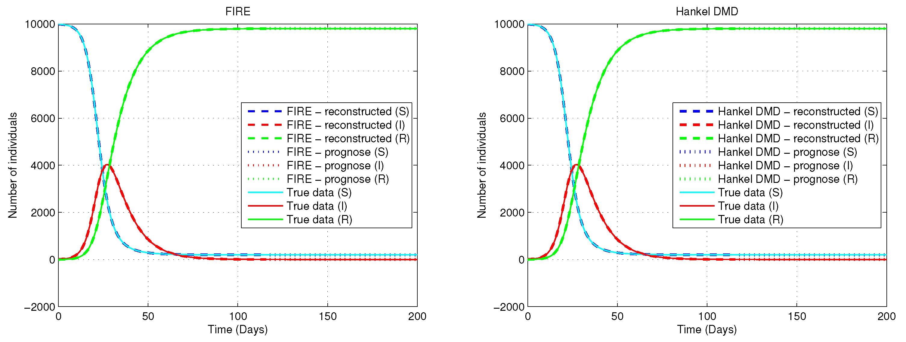
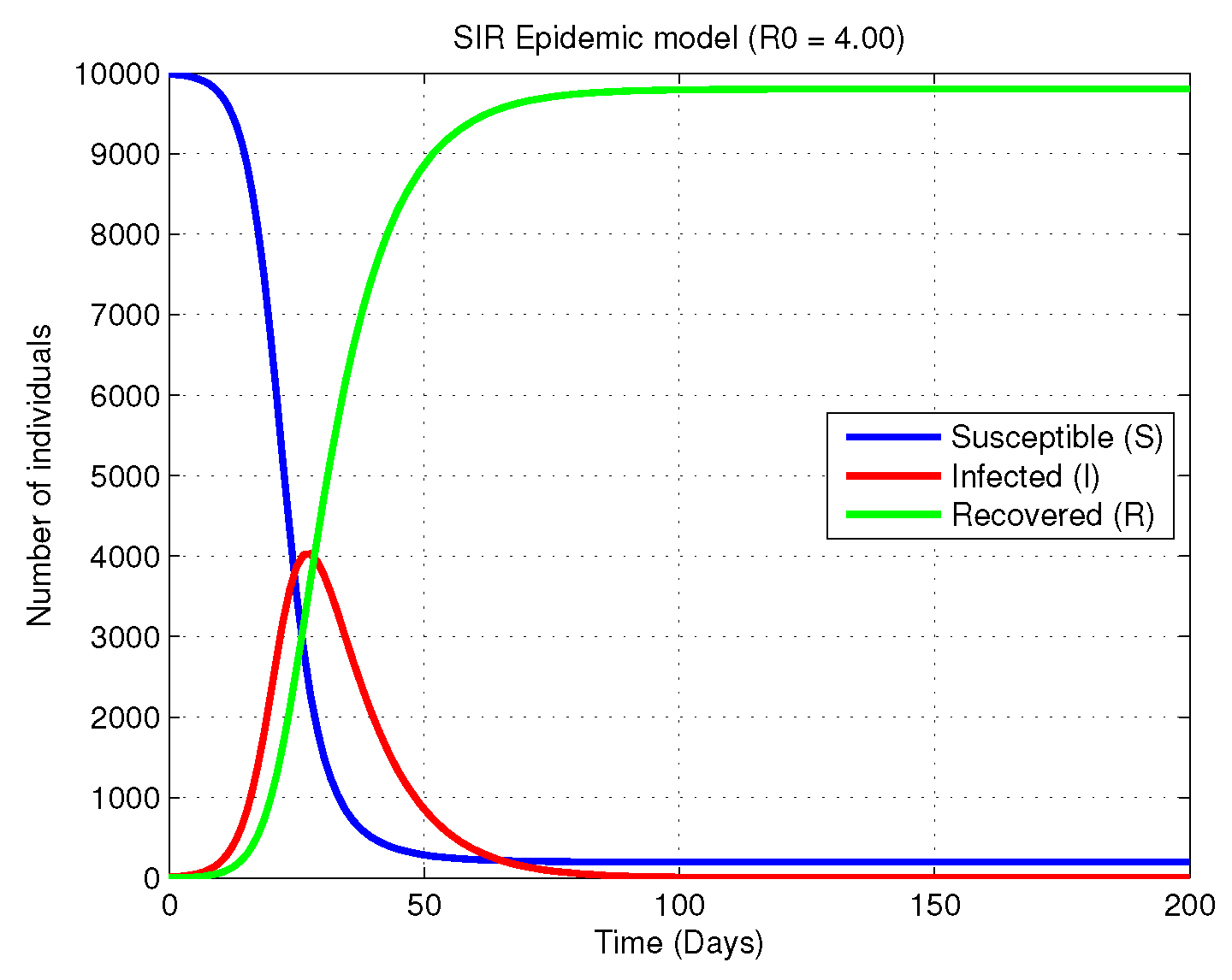
The numerical experiment is conducted with population size $N_p=10,000$ and initial conditions $I_0=10$, $R_0=0$, and $S_0=N_p-I_0$. The epidemiological parameters are set to $\beta =0.4$ and $\gamma =0.1$, yielding a basic reproduction number $R_0=\beta /\gamma =4.0$, corresponding to a pronounced epidemic growth regime. The system is simulated over a time horizon of $T_{\mathrm{end}}=200$ days using high-resolution temporal sampling with step size $\mathrm{\Delta }t$ to generate snapshot data. The resulting compartmental dynamics are shown in Figure 1.

Due to the bilinear coupling between the susceptible and infectious compartments, the SIR vector field is inherently nonlinear and non-normal. The generalized transfer operator $\mathcal{G}$ is therefore tasked with approximating the induced flow between epidemiological compartments via a linear evolution in an appropriately lifted feature space. By constructing a dictionary $\mathcal{D}$ of nonlinear observables, the proposed framework captures the dominant epidemic modes and provides a finite-dimensional linear representation of the underlying nonlinear dynamics.

To accurately capture the nonlinear interactions inherent in the SIR dynamics, we employ an augmented lifting dictionary that combines temporal delay embeddings with explicitly constructed nonlinear and differential features. This enriched representation enables the generalized transfer operator $\mathcal{G}$ to approximate the nonlinear epidemic flow by a linear evolution in a suitably high-dimensional feature space, where the dominant compartmental interactions are made explicit.

Let the population state be denoted by $\mathit{z}\left(t\right)={[z_1\left(t\right),z_2\left(t\right),z_3\left(t\right)]}^T$, where $z_1\left(t\right)=S\left(t\right)$, $z_2\left(t\right)=I\left(t\right)$, and $z_3\left(t\right)=R\left(t\right)$. The feature map $\mathrm{\Psi }$ is constructed by integrating three complementary sources of information:

• Temporal delay embedding (Hankel structure). We employ a delay depth of $s=24$, yielding a multi-step embedding that encodes the recent temporal history of the epidemic. This extended memory allows the operator to implicitly capture time-varying infection and recovery rates and enhances the identifiability of transient epidemic phases.
• Nonlinear interaction observables. Motivated by the bilinear infection term $SI$ in the governing equations, we explicitly incorporate cross-product observables of the following form:

  $${\psi }_1\left(t_k\right)=z_1\left(t_k\right)z_2\left(t_k\right),$$

  thereby embedding the dominant nonlinear coupling directly into the lifted space.
• Differential information. To further align the lifted dynamics with the underlying continuous-time structure, we augment the dictionary with a numerical approximation of the recovered population derivative:

  $$\dot{R}\approx {\displaystyle \frac{R_{k+1}-R_k}{\mathrm{\Delta }t}}.$$
  Since $\dot{R}=\gamma I$, this observable provides a direct linear proxy for the infectious compartment and substantially improves the spectral consistency of the learned operator. Accordingly, we include
  Since $\dot{R}=\gamma I$, this term provides a direct linear link to the infectious compartment, significantly improving the spectral alignment of the operator. We explicitly include observables,

  $${\psi }_2\left(t_k\right)={\displaystyle \frac{z_3\left(t_{k+1}\right)-z_3\left(t_k\right)}{dt}},$$

  as an additional feature.

Collectively, this construction yields an extended state space of dimension ${\mathcal{M}}^{25}$. The resulting lifted feature vector is given by

$$\mathit{\psi }\left(t_k\right)={[\mathit{z}\left(t_k\right),\dots ,\mathit{z}\left(t_{k+23}\right),{\psi }_1\left(t_k\right),\dots ,{\psi }_1\left(t_{k+23}\right),{\psi }_2\left(t_k\right),\dots ,{\psi }_2\left(t_{k+23}\right)]}^T,$$

so that, at each time step, the lifted state simultaneously encodes raw compartment values, nonlinear interaction terms, and differential information across all delay coordinates.

The data matrices are assembled via a standard time-shifting procedure,

$${\mathrm{\Psi }}_X=\left[\begin{array}{c}\mathit{\psi }\left(t_1\right),\dots ,\mathit{\psi }\left(t_T\right)\end{array}\right]\mathrm{a}\mathrm{n}\mathrm{d}{\mathrm{\Psi }}_Y=\left[\begin{array}{c}\mathit{\psi }\left(t_2\right),\dots ,\mathit{\psi }\left(t_{T+1}\right)\end{array}\right],$$

resulting in matrices of dimension $1024\times T$, with $T=120$ training snapshots. Applying Algorithm 1, we compute the finite-dimensional approximation G of the generalized transfer operator and use it to reconstruct the system dynamics.

Figure 2 compares the reconstructed SIR trajectories obtained using the proposed FIRE framework with those produced by the Hankel-DMD method.

The FIRE-based reconstruction closely follows the true nonlinear dynamics of all compartments, accurately reproducing both the transient growth phase and the decay regime of the infectious population. In particular, the timing and magnitude of the infection peak are well captured, indicating that the learned transfer operator successfully encodes the dominant nonlinear interaction mechanisms of the epidemic process.

Regularization and conditioning. The lifted regression problem arising in the SIR example is inherently high-dimensional, with a feature space dimension of $N=1024$ and only $T=120$ training snapshots. As a result, the estimation of the finite-dimensional transfer operator G from the relation ${\mathrm{\Psi }}_Y\approx G{\mathrm{\Psi }}_X$ is severely underdetermined and requires explicit regularization to ensure numerical stability and meaningful spectral properties.

In all numerical experiments, the operator G is computed using a truncated singular value decomposition (SVD) of the feature matrix ${\mathrm{\Psi }}_X$. Only the dominant singular directions are retained, corresponding to singular values satisfying ${\sigma }_j/{\sigma }_{max}\ge {10}^{-6}$. This procedure yields a regularized low-rank approximation of the regression operator and effectively filters spurious directions associated with noise and redundant observables. The singular value spectrum of ${\mathrm{\Psi }}_X$ exhibits rapid decay, revealing a strong intrinsic low-rank structure induced by the combined effect of delay embeddings and nonlinear interaction features. Importantly, the dominant eigenvalues of the learned operator are observed to be robust with respect to the chosen truncation threshold.

Although Tikhonov (ridge) regularization, (57) was not required for the results reported in this example, it remains a viable option for further stabilizing operator estimation in more severely ill-conditioned or noise-contaminated settings. In practice, SVD truncation alone proved sufficient to control conditioning and prevent overfitting.

To further assess numerical stability, we monitor the conditioning of the regression by examining the singular value decay of ${\mathrm{\Psi }}_X$ and the effective rank of the empirical Gram matrix ${\mathrm{\Psi }}_X{\mathrm{\Psi }}_X^{*}$. Despite the nominally large lifted dimension ($N\gg T$), the data-driven operator effectively acts on a substantially lower-dimensional subspace induced by the correlated temporal structure of the delay coordinates and nonlinear observables. This implicit dimensionality reduction enables stable operator identification and mitigates overfitting, even in the underdetermined regime.

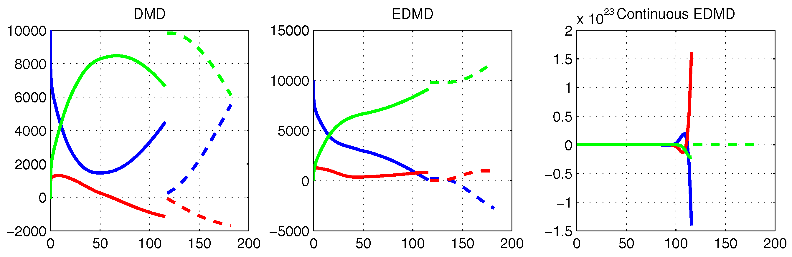
To provide a systematic comparison on the same simulated dataset, we evaluate several baseline methods, including Dynamic Mode Decomposition (DMD), Hankel DMD, Extended DMD (EDMD), and continuous-time EDMD (cEDMD). Among these approaches, Hankel DMD yields the best performance. While DMD, EDMD, and cEDMD fail to accurately reconstruct the nonlinear epidemic dynamics, Hankel DMD achieves a reconstruction error on the order of ${10}^{-4}$ when a delay dimension of $s=38$ is employed. The corresponding Hankel-DMD reconstruction is shown in Figure 2.

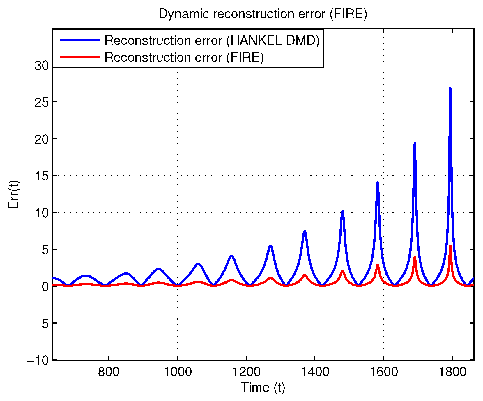
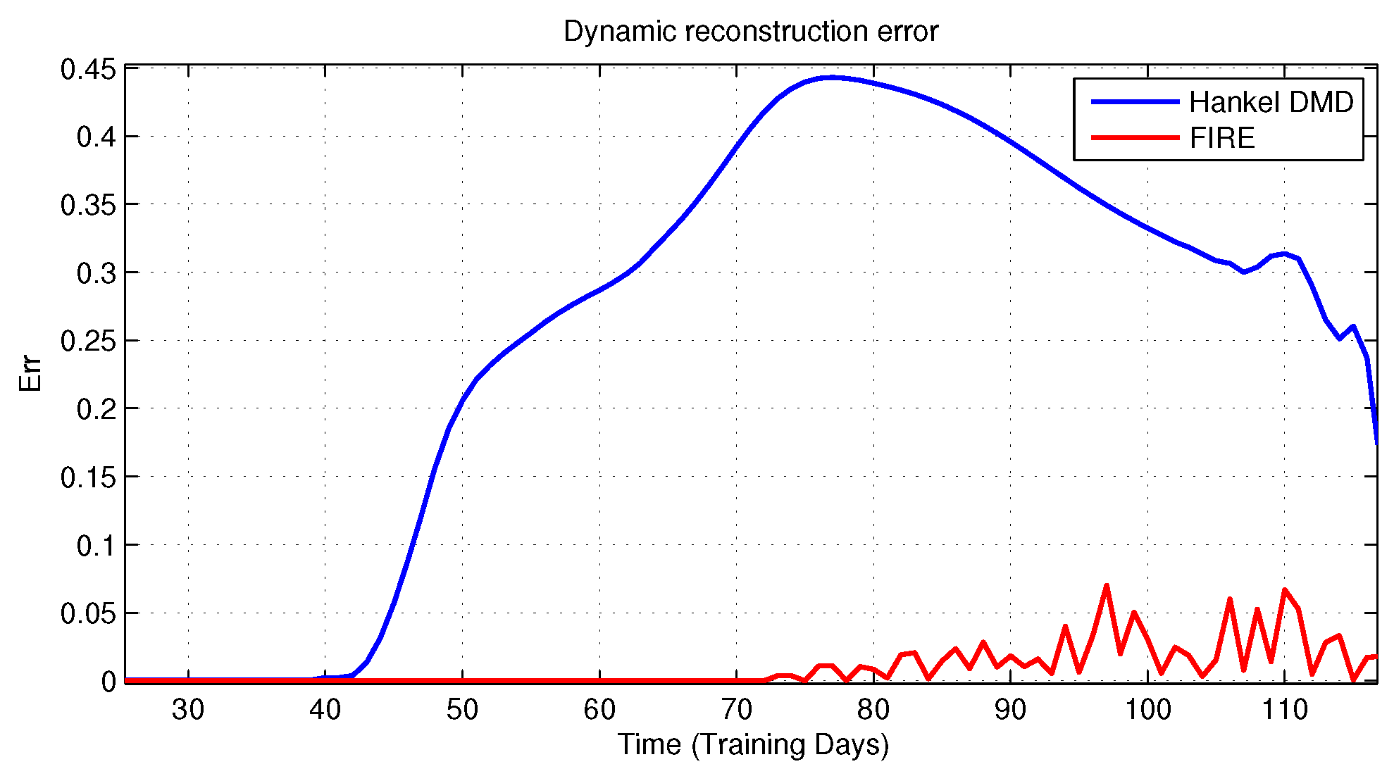
Reconstruction accuracy is quantified using the absolute pointwise error defined in (58). Figure 3 compares the temporal evolution of the reconstruction error for FIRE and Hankel DMD over the training interval. The FIRE framework consistently achieves a lower reconstruction error across all the time steps, with particularly pronounced improvements during the nonlinear growth and saturation phases of the epidemic.

For completeness, Figure 4 reports the reconstructions obtained using DMD, EDMD, and continuous EDMD. These methods fail to capture the essential nonlinear features of the SIR dynamics.

To provide a rigorous baseline comparison, the EDMD and continuous EDMD schemes were equipped with a comprehensive polynomial library, as follows:

$${\mathcal{D}}_{EDMD}=\{\mathit{z},{\mathit{z}}^2,z_1{z}_2,{\mathit{z}}^3,z_1^2{z}_2,z_1{z}_2^2\},$$

including all relevant cross-product terms up to the third order. For the continuous EDMD scheme, the evolution data matrix is constructed as

$$\begin{array}{cc}\hfill {\dot{\mathrm{\Psi }}}_{cEDMD}=[& \dot{\mathit{z}},2\mathit{z}\dot{\mathit{z}},{\dot{z}}_1{z}_2+z_1{\dot{z}}_2,3{\mathit{z}}^2\dot{\mathit{z}},\hfill \\ \hfill & 2z_1{\dot{z}}_1{z}_2+z_1^2{\dot{z}}_2,{\dot{z}}_1{z}_2^2+2z_1{z}_2{\dot{z}}_2],\hfill \end{array}$$

where the time derivatives are approximated using forward finite differences, as follows:

$$\dot{\mathit{z}}\left(t\right)\approx {\displaystyle \frac{\mathit{z}(t+\mathrm{\Delta }t)-\mathit{z}\left(t\right)}{\mathrm{\Delta }t}}.$$

The reconstruction quality is evaluated using the relative reconstruction error defined in (59).

Table 1. Relative reconstruction error (Err) of the SIR dynamics (60) for different methods.

	FIRE	DMD	Hankel DMD	EDMD	Continuous EDMD
Err	5.8914 × 10−5	0.5448	4.4415 × 10−4	0.4450	3.3922 × 1018

reports the errors for all methods considered.

Ablation Study. To isolate the contribution of each modeling component in the proposed FIRE framework, we perform an ablation study by systematically removing elements from the lifted representation. Specifically, we consider the following cases:

1.

Full dictionary: Delays + nonlinear cross-terms + derivative features.

2.

No delays: Remove temporal embeddings; retain nonlinear cross-terms and derivatives.

3.

No cross-terms: Remove nonlinear products $S·I$; retain delays and derivatives.

4.

No derivatives: Remove derivative features; retain delays and nonlinear cross-terms.

Table 2. Ablation results for the SIR example. The error is relative reconstruction error (59).

Dictionary	Relative Error ($\mathit{Err}$)
Full FIRE (delays + $S·I$ + $\dot{R}$)	5.8914 × 10−5
No delays ($S·I$ + $\dot{R}$)	4.2369 × 104
No nonlinear terms (delays + $\dot{R}$)	7.0787 × 10−4
No derivatives (delays + $S·I$)	7.0786 × 10−4
Pure delay (Hankel-DMD)	4.4415 × 10−4

reports the relative reconstruction error for different dictionary configurations.

The numerical results indicate that the explicit inclusion of the transmission nonlinearity ($S·I$) together with the recovered rate derivative $\dot{R}$ yields the highest reconstruction fidelity. By embedding the functional form of the infection mechanism directly into the observable space, the generalized operator $\mathcal{G}$ is able to accurately learn the transition from the initial exponential growth phase to the epidemic peak and the subsequent recovery regime. This hybrid strategy, which combines deep delay embeddings with physics-informed nonlinear observables, enables the proposed framework to significantly outperform standard DMD-based methods in both short- and long-term prediction accuracy.

From a theoretical perspective, this behavior is consistent with Takens’ embedding theorem, which guarantees that the topology of a finite-dimensional dynamical system can be reconstructed from a single observed time series given a sufficiently large delay window. The choice of a deep delay embedding with $s=24$ allows $\mathcal{G}$ to capture the delayed feedback between susceptible–infectious interactions and the ensuing peak in the infectious population. In effect, the operator implicitly encodes higher-order temporal dependencies that are not explicitly present in the original state variables, providing a fading memory representation of the epidemic dynamics.

By projecting the nonlinear flow onto a 120-dimensional extended observable space, the learned operator becomes markedly less sensitive to local numerical fluctuations in the sampled S, I, and R trajectories. This implicit regularization, induced by the delay structure and correlated nonlinear features, contributes to the observed robustness and accuracy of the FIRE reconstruction in highly nonlinear and transient regimes.

Example 2.

Forced Harmonic Oscillator with Transient Dynamics

A central challenge in data-driven system identification is the recovery of the underlying state space dynamics from limited, and often scalar, measurements. Classical operator-theoretic approaches typically rely on access to the full state or multiple observables and may fail to reconstruct the latent dynamical structure when only a single measurement is available. In contrast, the proposed generalized transfer operator $\mathcal{G}$ enables state reconstruction through a lifting strategy that combines delay embeddings with derivative-based observables, thereby recovering the intrinsic manifold from univariate time series data.

To assess the performance of $\mathcal{G}$ in this setting, we consider a second-order, linear, non-homogeneous dynamical system: a forced harmonic oscillator exhibiting both transient and steady-state behavior. The governing equation is

$$\ddot{z}+5z=sin\left(t\right)$$

(61)

where $z\left(t\right)$ denotes the displacement. The natural frequency of the unforced system is ${\omega }_0=\sqrt{5}\approx 2.236$ rad/s, while the external forcing acts at frequency $\omega =1$ rad/s. The coexistence of these frequencies induces a transient regime followed by a forced response, providing a nontrivial test case for operator-based identification from scalar data.

The trajectory is generated over the time interval $t\in [0,8]$ s, starting from rest with initial conditions $z\left(0\right)=0$ and $\dot{z}\left(0\right)=0$. The system is integrated using a variable-step Runge–Kutta method (ode45) with tight error tolerances ($\mathrm{RelTol}={10}^{-6}$, $\mathrm{AbsTol}={10}^{-6}$). A fixed sampling interval of $\mathrm{\Delta }t={10}^{-3}$ s yields 8001 discrete snapshots $\left\{z_k\right\}$, which capture both the initial transient phase and the subsequent forced oscillatory dynamics. This dataset serves as the sole input for constructing the data-driven approximation of the generalized operator $\mathcal{G}$.

In this experiment, we assume that only the scalar displacement signal $z\left(t\right)$ is available for measurement. The velocity $\dot{z}\left(t\right)$ and the external forcing are not directly observed. To compensate for this incomplete state information, we construct a compact yet expressive dictionary that embeds the scalar time series into a low-dimensional feature space enriched with derivative and forcing information. Our objective is to identify a continuous-time representation of the generalized transfer operator $\mathcal{G}$ via its infinitesimal generator.

Unlike discrete-time formulations, which approximate a finite-step evolution map, the generator-based approach seeks a linear operator G such that the lifted observables satisfy

$$\dot{\mathrm{\Psi }}\left(t_k\right)\approx G\mathrm{\Psi }\left(t_k\right),$$

(62)

where $\mathrm{\Psi }\left(t\right)$ denotes the feature map evaluated along the trajectory. This formulation directly approximates the action of the Lie generator associated with the underlying dynamics.

This example illustrates FIRE’s ability to operate on heterogeneous spaces, where the source space $\mathcal{X}$ and the target space $\mathcal{Y}$ are not identical. Specifically, $\mathcal{X}$ corresponds to a reconstructed feature space obtained from scalar measurements, while $\mathcal{Y}$ represents the infinitesimal evolution of these features under the system dynamics. The alignment between these spaces is achieved through a localized temporal window.

To this end, we introduce a symmetric delay structure with one step backward and one step forward, corresponding to memory depth $s=1$ and anticipation depth $q=1$. The resulting extended state at time index k is

$${\mathit{x}}_k={\left[z_{k-1},z_k,z_{k+1}\right]}^{\mathsf{T}}\in {\mathcal{M}}^3.$$

(63)

This local temporal window encodes sufficient information to approximate first- and second-order derivatives while remaining agnostic to the true physical state $(z,\dot{z})$.

From the windowed measurements (63), numerical derivatives are computed using centered finite differences:

$${\dot{z}}_{\mathrm{approx}}\left(t_k\right):={\displaystyle \frac{z_{k+1}-z_{k-1}}{2\mathrm{\Delta }t}},{\ddot{z}}_{\mathrm{approx}}\left(t_k\right):={\displaystyle \frac{z_{k+1}-2z_k+z_{k-1}}{\mathrm{\Delta }{t}^2}}.$$

(64)

These approximations provide local estimates of the velocity and acceleration without requiring explicit access to latent variables.

Based on this construction, we define a dictionary of observables $\mathcal{D}=\{{\psi }_1,\dots ,{\psi }_4\}$ acting on ${\mathit{x}}_k$ as

$${\psi }_1\left({\mathit{x}}_k\right)=z_k,{\psi }_2\left({\mathit{x}}_k\right)={\dot{z}}_{\mathrm{approx}}\left(t_k\right),{\psi }_3\left({\mathit{x}}_k\right)=sin\left(t_k\right),{\psi }_4\left({\mathit{x}}_k\right)=cos\left(t_k\right).$$

(65)

The inclusion of the trigonometric forcing terms explicitly encodes the non-autonomous input, while the derivative-based observable enables the reconstruction of the underlying second-order dynamics from the scalar data.

The use of the forward sample $z_{k+1}$ in the dictionary represents a localized anticipation depth during operator identification. Importantly, this non-causal information is required only in the offline training phase. Once the operator G is learned, the resulting spectral model is fully causal: the natural and forcing frequencies are embedded in the eigenvalues of G, enabling autonomous prediction without access to future measurements.

The resulting feature map is

$$\mathrm{\Psi }\left(t_k\right)=\left[\begin{array}{c}z\left(t_k\right)\\ {\dot{z}}_{\mathrm{approx}}\left(t_k\right)\\ sin\left(t_k\right)\\ cos\left(t_k\right)\end{array}\right],$$

with time derivative

$$\dot{\mathrm{\Psi }}\left(t_k\right)=\left[\begin{array}{c}{\dot{z}}_{\mathrm{approx}}\left(t_k\right)\\ {\ddot{z}}_{\mathrm{approx}}\left(t_k\right)\\ cos\left(t_k\right)\\ -sin\left(t_k\right)\end{array}\right],$$

where all derivatives are computed numerically from the sampled data.

Using the training dataset ${\{\mathrm{\Psi }\left(t_k\right),\dot{\mathrm{\Psi }}\left(t_k\right)\}}_{k=1}^T$ with $T=5600$ samples, we compute the continuous-time FIRE approximation by solving a least squares problem for the generator matrix $G\in {\mathbb{R}}^{4\times 4}$ in (62).

This dictionary design effectively “unfolds” the scalar signal $z\left(t\right)$ into a feature space in which the dynamics become linear and autonomous. By explicitly incorporating the driving terms $sin\left(t\right)$ and $cos\left(t\right)$ into the observable dictionary, the generalized operator $\mathcal{G}$ is able to represent the non-autonomous forcing without introducing explicit time dependence in the operator coefficients. As a result, the learned operator acts on an augmented state in which the external forcing is internalized as part of the state evolution.

We use the first 5600 snapshots as training data. The resulting operator matrix G, obtained from the least squares approximation $\dot{\mathrm{\Psi }}\approx G\mathrm{\Psi }$, provides a finite-dimensional numerical representation of the Lie generator associated with the lifted dynamics. This enables both high-fidelity state reconstruction and meaningful spectral analysis, demonstrating that the proposed framework remains robust even under the severe constraint of univariate measurements.

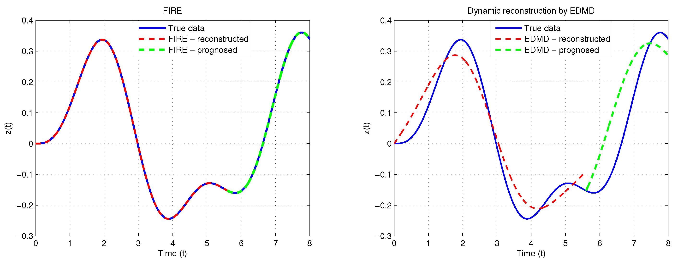
The dynamic reconstruction obtained using the FIRE algorithm is shown in Figure 5. For comparison, the right panel shows the reconstruction obtained using EDMD with a standard polynomial–trigonometric dictionary.

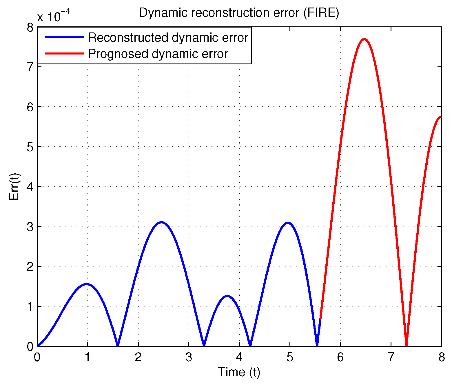
Figure 6 reports the pointwise absolute reconstruction error, computed using (58), for both the training interval and the out-of-sample prediction horizon. The observed error remains on the order of ${10}^{-4}$, with slightly increased deviations during the prediction phase, reflecting the extrapolative nature of the task.

To provide a rigorous benchmark, we compare FIRE against several standard data-driven decomposition methods: Dynamic Mode Decomposition (DMD), Hankel DMD, Extended DMD (EDMD), and continuous EDMD. Among these approaches, EDMD yields the best performance, although its reconstruction accuracy remains significantly inferior to that of FIRE.

A representative EDMD dictionary augmented with explicit forcing terms is given by

$${\mathcal{D}}_{EDMD}=\{z,z^2,z^3,sin\left(t\right),cos\left(t\right),1\}.$$

(66)

Despite the inclusion of cubic nonlinearities and trigonometric forcing, EDMD fails to accurately reconstruct the system dynamics, as illustrated in Figure 5.

For continuous EDMD, the same dictionary (66) is employed, with the corresponding evolution data matrix

$${\dot{\mathrm{\Psi }}}_{cEDMD}=[\dot{z},2z\dot{z},3z^2\dot{z},cos\left(t\right),-sin\left(t\right),0],$$

where time derivatives are approximated numerically.

Table 3. Relative reconstruction error for the forced oscillator (61).

	FIRE	DMD	Hankel DMD	EDMD	Continuous EDMD
Err	8.96 $\times {10}^{-4}$	$1.48$	$0.73$	$0.24$	$1.34$

summarizes the relative reconstruction errors (59) for all considered methods.

Unlike EDMD or Hankel-DMD, which rely on fixed temporal shifts within a single observable space, FIRE explicitly permits a general alignment map $\pi :\mathcal{X}\to \mathcal{Y}$ between heterogeneous spaces. In this example, the source space $\mathcal{X}$ encodes local temporal context through windowed scalar measurements, while the target space $\mathcal{Y}$ corresponds to the instantaneous evolution of lifted observables.

Consequently, the learned operator G is not a time-shift operator but a data-driven approximation of the infinitesimal generator governing the induced feature space dynamics. This distinction enables FIRE to recover hidden state information and non-autonomous forcing effects without requiring backward-time data or explicit access to the full system state. As a result, the proposed framework remains applicable in settings where classical Koopman-based methods either fail or require substantial modification.

Example 3.

Coupled Two-Mass Spring–Damper System

To demonstrate the effectiveness of the generalized transfer operator $\mathcal{G}$ in higher-dimensional state spaces, we consider a coupled two-degree of freedom (2-DOF) coupled system. The model consists of two masses, $m_1$ and $m_2$, coupled through a linear spring with stiffness k and a viscous damping element with coefficient c. This example illustrates the ability of the proposed framework to identify coupled dynamics and accurately capture unstable regimes using displacement-only measurements.

The governing equations of motion are given by the following coupled second-order ordinary differential equations:

$$\left\{\begin{array}{c}{m}_1{\ddot{z}}_1+c({\dot{z}}_1-{\dot{z}}_2)+k(z_1-z_2)=0,\hfill \\ m_2{\ddot{z}}_2+c({\dot{z}}_2-{\dot{z}}_1)+k(z_2-z_1)=0,\hfill \end{array}\right.$$

where $z_1\left(t\right)$ and $z_2\left(t\right)$ denote the displacements of masses $m_1$ and $m_2$, respectively.

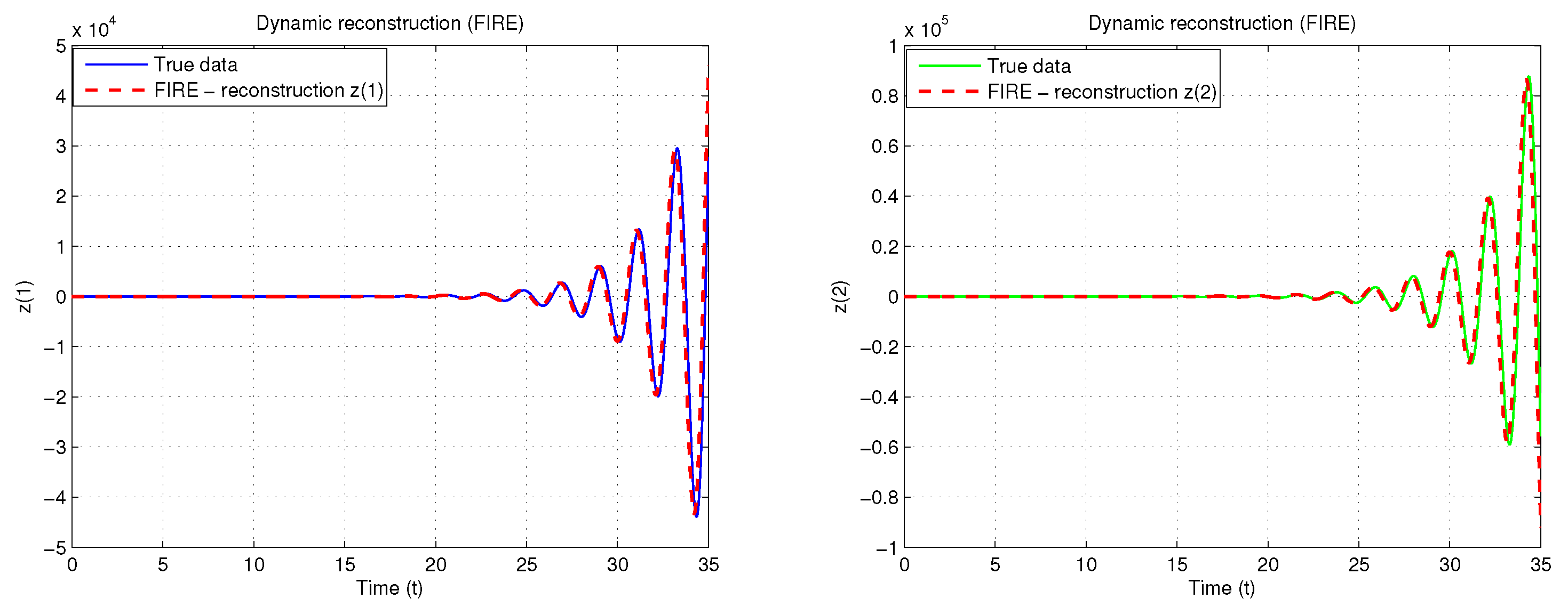
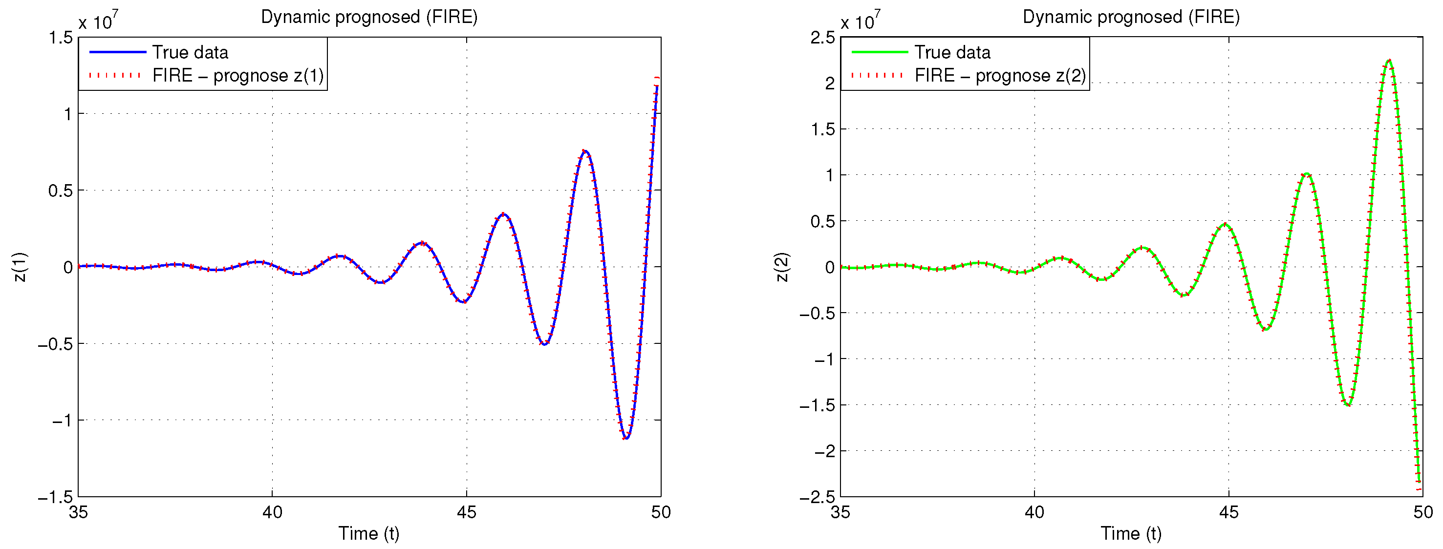
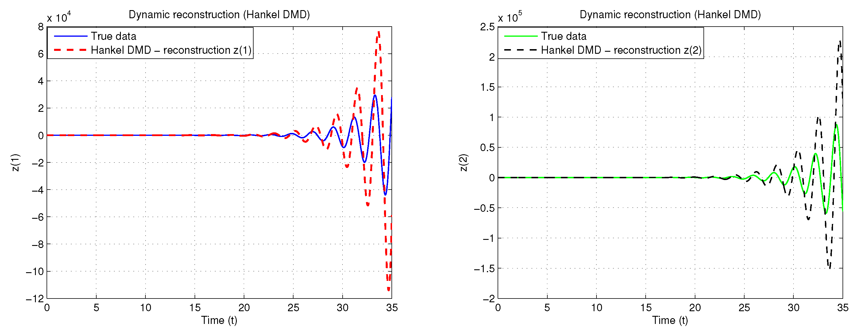
The numerical experiment is conducted using the parameters $m_1=2$, $m_2=1$, $k=6$, and $c=-0.5$. The system is simulated over the time interval $t\in [0,50]$ with time step $\mathrm{\Delta }t=0.01$ and initial condition ${\mathit{z}}_0={[1,1]}^T$, yielding 5001 discrete snapshots. The negative damping coefficient introduces an unstable regime in which energy is continuously injected into the system, causing exponential growth of oscillation amplitudes. This configuration provides a challenging test case for data-driven spectral identification methods.

The available measurements consist solely of the displacement vector $\mathit{z}\left(t\right)={[z_1\left(t\right),z_2\left(t\right)]}^T$. To construct the transfer operator $\mathcal{G}$, we lift these measurements into an augmented phase-space representation using forward finite differences. Let ${\mathit{z}}_k=\mathit{z}\left(t_k\right)$ denote the sampled displacement at time $t_k$. We define the extended state vectors as follows:

$${\mathit{x}}_k=[{\mathit{z}}_k;{\mathit{z}}_{k+1}],{\mathit{y}}_k=[{\mathit{z}}_{k+1};{\mathit{z}}_{k+2}],$$

which implies that the source and target spaces coincide, i.e., $\mathcal{X}\equiv \mathcal{Y}\equiv {\mathcal{M}}^4$.

Based on these windowed measurements, we define the lifted observables as follows:

$${\psi }_1\left(\mathit{z}\left(t_k\right)\right)={\mathit{z}}_k,{\psi }_2\left(\mathit{x}\left(t_k\right)\right)={\displaystyle \frac{{\mathit{z}}_{k+1}-{\mathit{z}}_k}{\mathrm{\Delta }t}},$$

resulting in the feature vector

$$\mathit{\psi }\left(t_k\right)=\left[\begin{array}{c}{\mathit{z}}_k\\ {\displaystyle \frac{{\mathit{z}}_{k+1}-{\mathit{z}}_k}{\mathrm{\Delta }t}}\end{array}\right],$$

which pairs displacement measurements with an approximation of the velocity. This lifting transforms the displacement-only observations into a phase space representation suitable for linear operator identification.

The first $70\%$ of the snapshots are used as training data for Algorithm 1. The reconstruction of the training trajectories obtained using FIRE is shown in Figure 7, while the out-of-sample predictions are presented in Figure 8.

The data matrices ${\mathrm{\Psi }}_X$ and ${\mathrm{\Psi }}_Y\in {\mathbb{R}}^{4\times T}$ are constructed by time-shifting the lifted features,

$${\mathrm{\Psi }}_X=\left[\begin{array}{c}\mathit{\psi }\left(t_1\right),\dots ,\mathit{\psi }\left(t_T\right)\end{array}\right],{\mathrm{\Psi }}_Y=\left[\begin{array}{c}\mathit{\psi }\left(t_2\right),\dots ,\mathit{\psi }\left(t_{T+1}\right)\end{array}\right],$$

where $T=3500$ denotes the number of training snapshots. This construction yields a finite-dimensional approximation of the discrete-time flow map in feature space.

The resulting operator G serves as a numerical approximation of the generalized transfer operator, mapping the current lifted state to its future counterpart. Despite the unstable nature of the underlying dynamics, the identified operator accurately captures both the inter-mass coupling and the dominant growth rates of the system modes, enabling reliable long-term prediction.

A comparative analysis was performed to benchmark the proposed FIRE scheme against several standard decomposition techniques, including DMD, Hankel DMD, Extended DMD (EDMD), and continuous EDMD. Among these methods, Hankel DMD provided the best performance, although still inferior to FIRE in terms of reconstruction fidelity.

For EDMD and continuous EDMD, we employ a nonlinear polynomial library:

$$D_{EDMD}=\{\mathit{z},{\mathit{z}}^2,z_1{z}_2,{\mathit{z}}^3,z_1^2{z}_2,z_1{z}_2^2\}.$$

The evolution data matrix for continuous EDMD is constructed as

$${\dot{\mathrm{\Psi }}}_{cEDMD}=[\dot{\mathit{z}},2\mathit{z}\dot{\mathit{z}},{\dot{z}}_1{z}_2+z_1{\dot{z}}_2,3{\mathit{z}}^2\dot{\mathit{z}},2z_1{\dot{z}}_1{z}_2+z_1^2{\dot{z}}_2,{\dot{z}}_1{z}_2^2+2z_1{z}_2{\dot{z}}_2],$$

where the time derivatives are approximated using forward finite differences:

$$\dot{\mathit{z}}\left(t\right)\approx {\displaystyle \frac{\mathit{z}(t+\mathrm{\Delta }t)-\mathit{z}\left(t\right)}{\mathrm{\Delta }t}}.$$

Hankel DMD achieves the best reconstruction among the classical methods when using a delay coefficient $s=2$. Figure 9 shows the training data reconstruction obtained by Hankel DMD.

Figure 10 depicts the pointwise absolute reconstruction error for both FIRE and Hankel DMD, computed according to Formula (58) over the training snapshots $i=1,\dots ,T$, with $T=3500$.

These results demonstrate that FIRE successfully reconstructs the full four-dimensional state trajectory, even under challenging conditions including coupled, unstable dynamics and limited measurements. The framework effectively captures the inter-mass coupling and reproduces the growth rates of the dominant modes, outperforming classical DMD-based methods and validating its robustness for high-dimensional, multi-component dynamical systems.

Example 4.

Spatio-Temporal Dynamics of a Nonlinear Soliton (PDE)

To demonstrate the applicability of the generalized transfer operator $\mathcal{G}$ in high-dimensional state spaces, we consider the evolution of a coherent structure governed by a partial differential equation. Specifically, we study the nonlinear Schrödinger (NLS) equation,

$$i{\displaystyle \frac{\partial q}{\partial t}}+{\displaystyle \frac{1}{2}}{\displaystyle \frac{{\partial }^{2}q}{\partial {\xi }^2}}+{\left|q\right|}^{2}q=0,$$

(67)

where $q(\xi ,t)$ is a complex-valued function of space $\xi$ and time t. Following [8], we perform a Fourier transform in space to obtain an evolution equation in the Fourier domain:

$${\displaystyle \frac{d\hat{q}}{dt}}=-{\displaystyle \frac{i}{2}}{k}^2\odot \hat{q}+{i\mathcal{F}\left(\right|q|}^2\odot q),$$

(68)

where ⊙ denotes element-wise multiplication, k is the vector of wavenumbers, and $\mathcal{F}$ represents the Fast Fourier Transform (FFT).

We discretize the spatial domain using $n=512$ points, resulting in a high-dimensional state space $\mathcal{M}\subset {\mathbb{C}}^{512}$. The initial condition is a high-amplitude soliton:

$$q(\xi ,0)=2sech\left(\xi \right),$$

and the system is integrated in time with a fourth-order Runge–Kutta scheme over $t\in [0,\pi )$, sampled at $M=21$ time points with $\mathrm{\Delta }t\approx 0.15$. The resulting dataset consists of a snapshot matrix $Z\in {\mathbb{C}}^{512\times 21}$ representing the spatio-temporal evolution of the soliton.

To capture the full dynamics, we employ a derivative-augmented dictionary. Each snapshot is paired with its temporal derivative approximated by forward differences, effectively doubling the dimensionality and allowing the operator to approximate the second-order-in-time nature of the NLS equation. Specifically, we define the extended state vectors as follows:

$${\mathit{x}}_k=[{\mathit{z}}_k;{\mathit{z}}_{k+1}],{\mathit{y}}_k=[{\mathit{z}}_{k+1};{\mathit{z}}_{k+2}],$$

so that the observation spaces satisfy $\mathcal{X}\equiv \mathcal{Y}\equiv {\mathcal{M}}^{2n}$, where $n=512$. The lifted observables are chosen as

$${\mathit{\psi }}_1\left({\mathit{x}}_k\right)={\mathit{z}}_k,{\mathit{\psi }}_2\left({\mathit{x}}_k\right)={\displaystyle \frac{{\mathit{z}}_{k+1}-{\mathit{z}}_k}{\mathrm{\Delta }t}},$$

yielding the feature vector $\mathrm{\Psi }\left({\mathit{x}}_k\right)={[{\mathit{\psi }}_1\left({\mathit{x}}_k\right),{\mathit{\psi }}_2\left({\mathit{x}}_k\right)]}^T$. The forward difference derivative approximates the velocity field at each spatial point:

$${\dot{\mathit{x}}}_k\approx {\displaystyle \frac{{\mathit{x}}_{k+1}-{\mathit{x}}_k}{\mathrm{\Delta }t}}={\mathit{\psi }}_2\left({\mathit{x}}_k\right),$$

providing the operator with information about the temporal evolution of the system.

Finally, the lifted snapshot matrices are constructed as

$${\mathrm{\Psi }}_X=[\mathit{\psi }\left({\mathit{x}}_1\right),\dots ,\mathit{\psi }\left({\mathit{x}}_M\right)],{\mathrm{\Psi }}_Y=[\mathit{\psi }\left({\mathit{y}}_1\right),\dots ,\mathit{\psi }\left({\mathit{y}}_M\right)],$$

with dimensions 1024 × 19. Using Algorithm 1, we compute the finite-dimensional approximation of the transfer operator G, which simultaneously provides the reconstructed state vectors and the corresponding eigenfunctions and eigenvalues of the high-dimensional nonlinear system.

To evaluate the performance of the proposed generalized transfer operator $\mathcal{G}$, we conducted a comparative study against standard decomposition techniques: Dynamic Mode Decomposition (DMD), Hankel DMD, Extended DMD (EDMD), and continuous EDMD (cEDMD). Figure 11 depicts the full simulation data along with reconstructions obtained by the FIRE algorithm and Hankel DMD.

The accuracy of the reconstructions is quantified using the pointwise absolute error metric (58). Continuous EDMD exhibited the poorest performance and is not visualized here. Among the remaining methods, FIRE and Hankel DMD consistently produce the lowest reconstruction errors, as shown in Figure 12.

Hankel DMD achieves its best performance using a temporal stack of only two snapshots, highlighting the importance of encoding velocity information in the feature space. For EDMD, we employed a dictionary consistent with the cubic nonlinearity of the NLS equation:

$$\mathit{\psi }\left(\mathit{z}\right)={[\mathit{z},|\mathit{z}|}^2{\mathit{z}]}^T.$$

Despite this, the FIRE algorithm provides superior reconstruction, demonstrating the advantage of a carefully designed, derivative-augmented observable set.

The eigenvalue spectra computed by the different methods further illustrate the efficacy of FIRE (Figure 13). FIRE aligns the eigenvalues close to the imaginary axis, as expected for the Hamiltonian-like dynamics of the soliton, whereas deviations are observed for DMD and EDMD.

The inclusion of the derivative $\dot{\mathit{x}}$ in the dictionary is essential for PDE systems. It allows the operator G to account for the “momentum” of the wave field, effectively capturing the spatio-temporal evolution even with a limited number of temporal snapshots ($M=21$). This lifting enables the extraction of dominant Koopman modes that characterize the soliton’s stability and shape-preserving propagation, demonstrating the robustness of the proposed framework for distributed parameter systems with continuous-state fields.

6. Conclusions

Standard Koopman-based approaches approximate the evolution operator by projecting the dynamics onto a finite set of observables defined at single time instances. However, many dynamical systems exhibit memory effects, delays, or spatio-temporal dependencies that cannot be adequately captured by single-state observables.

In this work, we introduce a multi-state extension in which each observable depends on multiple system states over time, forming a richer feature space that captures temporal dependencies more effectively. Moreover, the construction of the target data in feature space is generalized to allow functions of multiple observables, enabling more flexible regression and mode extraction. Importantly, the framework retains interpretability: the eigenvalues of the operator characterize temporal scales, while the corresponding modes represent spatial or state patterns. This multi-state formulation improves reconstruction accuracy, captures temporal correlations, and is applicable to both ODE and PDE systems.

The main contributions of this work can be summarized as follows:

• We generalize the feature space target data to allow functions of multi-state observables, increasing the expressivity of Koopman approximations.
• We introduce a multi-state extension of the EDMD framework, in which observables are functions of sequences of system states rather than a single state.
• We provide numerical demonstrations on canonical nonlinear systems, showing improved reconstruction and spectral representation compared to standard EDMD.

The advantages of this framework include its ability to capture temporal correlations and memory effects, its improved representation of nonlinear dynamics, and its applicability to high-dimensional PDE systems. Numerical experiments confirm its effectiveness in reconstructing system trajectories and identifying dominant features, suggesting its potential for applications in model reduction, prediction, and control of complex dynamical systems.

Overall, the proposed framework unifies classical Koopman theory, delay embeddings, temporal convolution models, and modern sequence-learning architectures, offering a principled linear-operator perspective for systems with memory, multi-resolution dynamics, or nonlocal temporal dependencies. This approach opens new avenues for data-driven analysis of systems with temporal correlations, memory effects, or spatial couplings, bridging the gap between traditional DMD/EDMD methods and the dynamics of multi-step or coupled systems.

References

1. Koopman, B.O. Hamiltonian systems and transformation in hilbert space. Proc. Natl. Acad. Sci. USA 1931, 17, 315–318. [Google Scholar] [CrossRef]
2. Koopman, B.O.; Neumann, J.v. Dynamical systems of continuous spectra. Proc. Natl. Acad. Sci. USA 1932, 18, 255. [Google Scholar]
3. Mezić, I. Spectral properties of dynamical systems, model reduction and decompositions. Nonlinear Dyn. 2025, 41, 309–325. [Google Scholar]
4. Budišić, M.; Mezić, I. Geometry of the ergodic quotient reveals coherent structures in flows. Phys. D Nonlinear Phenom. 2012, 241, 1255–1269. [Google Scholar] [CrossRef]
5. Budišić, M.; Mohr, R.; Mezixcx, I. Applied Koopmanism. Chaos Interdiscip. J. Nonlinear Sci. 2012, 22, 047510. [Google Scholar] [CrossRef] [PubMed]
6. Schmid, P.J. Dynamic mode decomposition of numerical and experimental data. J. Fluid Mech. 2010, 656, 5–28. [Google Scholar] [CrossRef]
7. Tu, J.H.; Rowley, C.W.; Luchtenburg, D.M.; Brunton, S.L.; Kutz, J.N. On dynamic mode decomposition: Theory and applications. J. Comput. Dyn. 2014, 1, 391–421. [Google Scholar] [CrossRef]
8. Kutz, J.N.; Brunton, S.L.; Brunton, B.W.; Proctor, J.L. Dynamic Mode Decomposition: Data-Driven Modeling of Complex Systems; Society for Industrial and Applied Mathematics (SIAM): Philadelphia, PA, USA, 2016; pp. 1–234. ISBN 978-1-611-97449-2. [Google Scholar]
9. Brunton, B.W.; Johnson, L.A.; Ojemann, J.G.; Kutz, J.N. Extracting spatial–temporal coherent patterns in large-scale neural recordings using dynamic mode decomposition. J. Neurosci. Methods 2016, 258, 1–15. [Google Scholar]
10. Proctor, J.L.; Eckhoff, P.A. Discovering dynamic patterns from infectious disease data using dynamic mode decomposition. Int. Health 2015, 7, 139–145. [Google Scholar] [CrossRef]
11. Grosek, J.; Kutz, J.N. Dynamic Mode Decomposition for Real-Time Background/Foreground Separation in Video. arXiv 2014, arXiv:1404.7592. [Google Scholar]
12. Mann, J.; Kutz, J.N. Dynamic mode decomposition for financial trading strategies. Quant. Financ. 2016, 16, 1643–1655. [Google Scholar] [CrossRef]
13. Kuttichira, D.P.; Gopalakrishnan, E.A.; Menon, V.K.; Soman, K.P. Stock price prediction using dynamic mode decomposition. In Proceedings of the 2017 International Conference on Advances in Computing, Communications and Informatics (ICACCI), Udupi, India, 13–16 September 2017; pp. 55–60. [Google Scholar] [CrossRef]
14. Berger, E.; Sastuba, M.; Vogt, D.; Jung, B.; Amor, H.B. Estimation of perturbations in robotic behavior using dynamic mode decomposition. J. Adv. Robot. 2015, 29, 331–343. [Google Scholar] [CrossRef]
15. Mezić, I. Analysis of fluid flows via spectral properties of the Koopman operator. Annu. Rev. Fluid Mech. 2013, 45, 357–378. [Google Scholar] [CrossRef]
16. Bai, Z.; Kaiser, E.; Proctor, J.L.; Kutz, J.N.; Brunton, S.L. Dynamic Mode Decomposition for Compressive System Identification. AIAA J. 2020, 58, 561–574. [Google Scholar] [CrossRef]
17. Le Clainche, S.; Vega, J.M.; Soria, J. Higher order dynamic mode decomposition of noisy experimental data: The flow structure of a zero-net-mass-flux jet. Exp. Therm. Fluid Sci. 2017, 88, 336–353. [Google Scholar] [CrossRef]
18. Li, B.; Garicano-Menaab, J.; Valero, E. A dynamic mode decomposition technique for the analysis of non-uniformly sampled flow data. J. Comput. Phys. 2022, 468, 111495. [Google Scholar] [CrossRef]
19. Jovanović, M.R.; Schmid, P.J.; Nichols, J.W. Sparsity-promoting dynamic mode decomposition. Phys. Fluids 2014, 26, 024103. [Google Scholar] [CrossRef]
20. Mezić, I. On Numerical Approximations of the Koopman Operator. Mathematics 2022, 10, 1180. [Google Scholar] [CrossRef]
21. Nedzhibov, G. Extended Online DMD and Weighted Modifications for Streaming Data Analysis. Computation 2023, 11, 114. [Google Scholar] [CrossRef]
22. Williams, M.O.; Kevrekidis, I.G.; Rowley, C.W. A data–driven approximation of the koopman operator: Extending dynamic mode decomposition. J. Nonlinear Sci. 2015, 25, 1307–1346. [Google Scholar] [CrossRef]
23. Arbabi, H.; Mezić, I. Ergodic theory, dynamic mode decomposition, and computation of spectral properties of the Koopman operator. SIAM J. Appl. Dyn. Syst. 2017, 16, 2096–2126. [Google Scholar] [CrossRef]
24. Brunton, S.L.; Brunton, B.W.; Proctor, J.L.; Kaiser, E.; Kutz, J.N. Chaos as an intermittently forced linear system. Nat. Commun. 2017, 8, 19. [Google Scholar] [CrossRef]
25. Nedzhibov, G.H. Delay-Embedding Spatio-Temporal Dynamic Mode Decomposition. Mathematics 2024, 12, 762. [Google Scholar] [CrossRef]
26. Proctor, J.L.; Brunton, S.L.; Kutz, J.N. Dynamic mode decomposition with control. SIAM J. Appl. Dyn. Syst. 2016, 15, 142–161. [Google Scholar] [CrossRef]
27. Nedzhibov, G. An Improved Approach for Implementing Dynamic Mode Decomposition with Control. Computation 2023, 11, 201. [Google Scholar] [CrossRef]
28. Nedzhibov, G. An Alternative Framework for Dynamic Mode Decomposition with Control. AppliedMath 2025, 5, 60. [Google Scholar] [CrossRef]
29. Askham, T.; Kutz, J.N. Variable projection methods for an optimized dynamic mode decomposition. SIAM J. Appl. Dyn. Syst. 2018, 17, 380–416. [Google Scholar] [CrossRef]
30. Dawson, S.T.M.; Hemati, M.S.; Williams, M.O.; Rowley, C.W. Characterizing and correcting for the effect of sensor noise in the dynamic mode decomposition. Exp. Fluids 2016, 57, 42. [Google Scholar] [CrossRef]
31. Korda, M.; Mezić, I. Linear predictors for nonlinear dynamical systems: Koopman operator meets model predictive control. Automatica 2018, 93, 149–160. [Google Scholar] [CrossRef]
32. Williams, M.O.; Rowley, C.W.; Kevrekidis, I.G. A kernel approach to data-driven Koopman spectral analysis. J. Comput. Dyn. 2015, 2, 247–265. [Google Scholar] [CrossRef]
33. Anantharamu, S.; Mahesh, K. A parallel and streaming Dynamic Mode Decomposition algorithm with finite precision error analysis for large data. J. Comput. Phys. 2019, 380, 355–377. [Google Scholar] [CrossRef]
34. Maryada, K.R.; Norris, S.E. Reduced-communication parallel dynamic mode decomposition. J. Comput. Sci. 2022, 61, 101599. [Google Scholar] [CrossRef]
35. Smith, E.; Variansyah, I.; McClarren, R. Variable Dynamic Mode Decomposition for Estimating Time Eigenvalues in Nuclear Systems. arXiv 2022, arXiv:2208.10942v1. [Google Scholar]
36. Ngo, T.T.; Nguyen, V.; Pham, X.Q.; Hossain, M.A.; Huh, E.N. Motion Saliency Detection for Surveillance Systems Using Streaming Dynamic Mode Decomposition. Symmetry 2020, 12, 1397. [Google Scholar] [CrossRef]
37. Duran-Siguenza, J.F.; Minchala, L.I.; Garza-Castanon, L.E.; Zhang, H. Control based on the Koopman operator: A comprehensive review. J. Frankl. Inst. 2025, 362, 108256. [Google Scholar] [CrossRef]
38. Islam, M.S.; Ahmad, M.A. Data-driven continuous-time Hammerstein modeling with missing data using improved Archimedes optimization algorithm. Results Eng. 2024, 24, 103357. [Google Scholar] [CrossRef]
39. Chu, B.; Rapisarda, P. Data-Driven Iterative Learning Control for Continuous-Time Systems. In Proceedings of the 2023 62nd IEEE Conference on Decision and Control (CDC), Singapore, 13–15 December 2023; pp. 4626–4631. [Google Scholar]
40. Beykal, B.; Diangelakis, N.A.; Pistikopoulos, E.N. Continuous-Time Surrogate Models for Data-Driven Dynamic Optimization; Montastruc, L., Negny, S., Eds.; Computer Aided Chemical Engineering; Elsevier: Amsterdam, The Netherlands, 2022; Volume 51, pp. 205–210. [Google Scholar]
41. Takens, F. Detecting strange attractors in turbulence. Lect. Notes Math. 1981, 898, 366–381. [Google Scholar]
42. Brunton, S.L.; Budišić, M.; Kaiser, E.; Kutz, J.N. Modern Koopman Theory for Dynamical Systems. arXiv 2021, arXiv:2102.12086. [Google Scholar] [CrossRef]
43. Klus, S.; Nüske, F.; Koltai, P.; Wu, H.; Kevrekidis, I.; Schutte, C.; Noe, F. Data-driven model reduction and transfer operator approximation. J. Nonlinear Sci. 2018, 28, 985–1010. [Google Scholar] [CrossRef]
44. Otto, S.E.; Rowley, C.W. Koopman operators for estimation and control of dynamical systems. Annu. Rev. Control Robot. Auton. Syst. 2021, 4, 59–87. [Google Scholar] [CrossRef]
Figure 1. Time evolution of the SIR epidemic model with reproduction number R 0 = 4 .
Mathematics 14 00464 g001
Figure 2. Reconstruction of SIR dynamics using FIRE (left) and Hankel-DMD (right).
Mathematics 14 00464 g002
Figure 3. Pointwise reconstruction error (58) for the SIR model using FIRE and Hankel DMD.
Mathematics 14 00464 g003
Figure 4. Dynamic reconstruction of the SIR model using DMD, EDMD, and continuous EDMD. The state variables are shown as follows: susceptible S (blue), infected I (red), and recovered R (green).
Mathematics 14 00464 g004
Figure 5. Dynamics governed by Equation (61). Reconstruction by FIRE (left) and by EDMD (right).
Mathematics 14 00464 g005
Figure 6. Pointwise reconstruction error for training and predicted trajectories obtained by FIRE.
Mathematics 14 00464 g006
Figure 7. Dynamic reconstruction of the training data obtained using FIRE.
Mathematics 14 00464 g007
Figure 8. Dynamic reconstruction of the prognosed trajectories obtained using FIRE.
Mathematics 14 00464 g008
Figure 9. Dynamic reconstruction of training data using Hankel DMD.
Mathematics 14 00464 g009
Figure 10. Pointwise reconstruction error for FIRE and Hankel DMD.
Mathematics 14 00464 g010
Figure 11. Spatio-temporal dynamics of the NLS soliton (67): full simulation data (left), reconstruction by FIRE (middle), and reconstruction by Hankel DMD (right).
Mathematics 14 00464 g011
Figure 12. Pointwise reconstruction error (58) for DMD, Hankel DMD, EDMD, and FIRE.
Mathematics 14 00464 g012
Figure 13. Eigenvalue spectra computed by FIRE, Hankel DMD, DMD, and EDMD.
Mathematics 14 00464 g013