Article

Training Agents for Strategic Curling Through a Unified Reinforcement Learning Framework

1
Department of Computer Engineering, Hankuk University of Foreign Studies, Seoul 02450, Republic of Korea
2
Department of Sport Medicine & Rehabilitation, Kyungil University, Gyeongsan 38428, Republic of Korea
*
Author to whom correspondence should be addressed.
Mathematics 2026, 14(3), 403; https://doi.org/10.3390/math14030403
Submission received: 3 December 2025 / Revised: 22 January 2026 / Accepted: 22 January 2026 / Published: 23 January 2026
(This article belongs to the Special Issue Applications of Intelligent Game and Reinforcement Learning)

Abstract

Curling presents a challenging continuous-control problem in which shot outcomes depend on long-horizon interactions between complex physical dynamics, strategic intent, and opponent responses. Despite recent progress in applying reinforcement learning (RL) to games and sports, curling lacks a unified environment that jointly supports stable, rule-consistent simulation, structured state abstraction, and scalable agent training. To address this gap, we introduce a comprehensive learning framework for curling AI, consisting of a full-sized simulation environment, a task-aligned Markov decision process (MDP) formulation, and a two-phase training strategy designed for stable long-horizon optimization. First, we propose a novel MDP formulation that incorporates stone configuration, game context, and dynamic scoring factors, enabling an RL agent to reason simultaneously about physical feasibility and strategic desirability. Second, we present a two-phase curriculum learning procedure that significantly improves sample efficiency: Phase 1 trains the agent to master delivery mechanics by rewarding accurate placement around the tee line, while Phase 2 transitions to strategic learning with score-based rewards that encourage offensive and defensive planning. This staged training stabilizes policy learning and reduces the difficulty of direct exploration in the full curling action space. We integrate this MDP and training procedure into a unified Curling RL Framework, built upon a custom simulator designed for stability, reproducibility, and efficient RL training and a self-play mechanism tailored for strategic decision-making. Agent policies are optimized using Soft Actor–Critic (SAC), an entropy-regularized off-policy algorithm designed for continuous control. As a case study, we compare the learned agent’s shot patterns with elite match records from the men’s division of the Le Gruyère AOP European Curling Championships 2023, using 6512 extracted shot images. Experimental results demonstrate that the proposed framework learns diverse, human-like curling shots and outperforms ablated variants across both learning curves and head-to-head evaluations. Beyond curling, our framework provides a principled template for developing RL agents in physics-driven, strategy-intensive sports environments.

1. Introduction

Curling is an Olympic sport in which two teams take turns executing shots, requiring both precision and strategic decision-making. First included in the 1924 Winter Olympics in Chamonix, curling has since developed into a highly tactical sport with a rich history [1].
Victory in curling depends on more than just strength and accuracy. Players must precisely control the stone’s speed and rotation while considering friction, collisions, and ice conditions. Strategic shot placement is key, whether to obstruct the opponent’s stones or secure an advantageous position. Since each shot affects the game’s progression, players must balance immediate gains with long-term strategy.
Curling involves strategic considerations such as hammer usage and cumulative scoring dynamics (e.g., blank ends). However, in this study we focus on strategic decision-making within a single end. We model one end as an episodic Markov Decision Process (MDP) with a fixed horizon of 16 deliveries (8 per team). Even under this single-end setting, the problem remains challenging because each shot can have delayed and collision outcomes, creating long-horizon credit assignment over the remaining deliveries. Addressing these challenges motivates the development of a dedicated reinforcement learning (RL) framework tailored to the structure and strategic demands of curling.
In recent years, AI has demonstrated remarkable success in analyzing and optimizing strategies across various games and sports [2]. In intellectual sports, AI systems have already surpassed human expertise and provided new forms of strategic insight [3]. Google’s AlphaGo and AlphaGo Zero, for example, defeated world-class Go professionals and transformed modern Go training [4,5]. Similarly, Microsoft’s Suphx—a mahjong AI combining supervised learning with RL—has outperformed 99.99% of players on the competitive Tenhou platform [6]. Kuaishou’s DouZero has likewise achieved strong performance in Fighting the Landlord, surpassing hundreds of competing AI agents and demonstrating human-level competence despite the stochastic nature of the game [7]. More recently, deep reinforcement learning (DRL) approaches have been applied to curling [8,9], indicating growing interest in strategic shot-planning for this domain.
Despite this progress, applying deep reinforcement learning (DRL) to curling presents several distinctive challenges. First, an RL-compatible curling simulator must (i) maintain physically plausible dynamics while remaining computationally stable; and (ii) expose learning-relevant internal state variables, such as stone positions, velocities, and collision events, in a consistent and analyzable form. Although perfect physical replication is not the goal of this study, a simulator that is consistent, fully observable, and reproducible is a critical prerequisite for methodological development in curling. Second, beyond simulation fidelity, curling requires long-horizon and hierarchical reasoning: each shot influences not only the immediate scoring outcome but also the future tactical landscape within an end, where each shot shapes the later tactical landscape (e.g., setting guards or preparing for the final hammer shot) under delayed rewards. Effective agents must therefore learn to integrate short-term shot execution with long-term strategic planning under delayed rewards.
These challenges make curling a demanding problem for DRL-based decision-making. Developing an effective agent requires accurate physical simulation and sequential decision-making under uncertainty. Unlike board games such as chess or Go, curling involves continuous action spaces (e.g., shot speed, angle, and rotation) and dynamic environmental interactions (e.g., ice friction and stone collisions). These factors make DRL- and model-based planning particularly effective for optimizing shot selection and adapting to evolving game conditions.
To overcome these limitations, search-based methods such as Monte Carlo Tree Search (MCTS) [10] have been applied. MCTS has demonstrated high performance in strategic games like chess and Go by probabilistically exploring decision paths to identify optimal actions. However, applying traditional MCTS to curling is challenging due to its continuous action space and inherent uncertainty. Unlike board games with discrete moves, curling requires selecting precise shot parameters, including speed, angle, and rotation. Yee et al. [11] extended upper confidence trees [12] with the Kernel Regression UCT (KR-UCT) algorithm, allowing information sharing among similar actions to improve decision-making in continuous spaces. Their results showed that KR-UCT outperformed conventional MCTS by efficiently exploring promising action regions beyond predefined shot candidates. Despite these advancements, Monte Carlo-based search methods remain computationally expensive, requiring a large number of simulations. Furthermore, since MCTS re-executes the search from scratch at each turn, it cannot retain learning from past experiences unless identical situations arise.
Recent advancements in DRL have opened new possibilities for curling strategy optimization [8,9,13,14,15]. Unlike rule-based or search-based methods, DRL enables agents to learn optimal strategies through self-play and experience, without relying on predefined heuristics. With sufficient training, DRL has the potential to surpass human decision-making. However, its application to curling presents challenges, including the complexity of building a stable, rule-consistent simulator, the continuous action space, and sparse rewards, as points are only awarded at the end of an end. D. Won et al. [13] framed curling as a real-world AI challenge and proposed an adaptive DRL. Their key innovation was integrating temporal features into DRL algorithms, enabling the agent to adapt to changing ice conditions. Their agent, Curly, refined shot decisions using accumulated game data, significantly improving accuracy. In experimental matches, Curly won three out of four games against South Korea’s national teams, demonstrating DRL’s potential to bridge the gap between simulation and real-world performance. Despite its potential, DRL requires significant computational resources and training time. Additionally, learned policies often lack interpretability, making AI-driven decisions difficult to analyze. To mitigate these challenges, DRL is often integrated with traditional search and simulation techniques, improving stability and serving as a step toward fully autonomous DRL-driven curling strategies. Further advancements in self-play learning have been explored in curling AI. Y. Han et al. [8] applied Neural Fictitious Self-Play (NFSP) [15], where two neural networks were alternately trained through repeated self-play. To handle curling’s continuous action space, they integrated NFSP with KR-UCT, allowing the policy network to encode strategic knowledge while reducing reliance on computationally expensive MCTS searches. However, their study highlighted the challenges of achieving optimal strategies solely through end-to-end deep learning due to learning instability and the complexity of function approximation in continuous spaces. Junjie Lin et al. [9] combined RL with decision trees using Distributed Proximal Policy Optimization (PPO). They first constructed a decision tree based on domain knowledge, then refined it through DRL to enhance generalization while maintaining interpretability and stability. This method won the 2022 RLChina curling competition with a record of 31 wins, 19 draws, and 0 losses. However, if the initial decision tree is inaccurate, PPO may struggle with inefficient exploration. Additionally, DRL does not automatically correct flaws in the tree, requiring manual adjustments. PPO’s clipping mechanism, while stabilizing training, can also limit the model’s ability to learn highly flexible strategies.
To address these limitations, we introduce a unified reinforcement learning framework for curling, designed to provide a complete pipeline spanning environment modeling, MDP formulation, and agent training. Unlike previous methods that depend on discretized action spaces or handcrafted decision structures, our framework directly supports continuous shot-level control, enabling direct continuous control of release force, angle, and rotation without discretizing the action space. The framework is built on a custom curling simulator specifically developed for RL research, providing stable stone dynamics, configurable rules, and full access to internal states necessary for systematic analysis and reproducible benchmarking.
Central to the framework is a new curling-specific MDP formulation that incorporates continuous actions, physically grounded state representations, and a reward structure aligned with tactical objectives within an end. This MDP allows agents to learn both offensive and defensive behaviors by anticipating opponent responses over the remaining shots in the current end. Furthermore, we introduce a two-phase training strategy: Phase 1 focuses on establishing low-level shot consistency by learning to deliver stones accurately toward the tee line, while Phase 2 optimizes end-level scoring through reward shaping based on strategic outcomes. This staged learning procedure stabilizes policy acquisition and mitigates the difficulty of sparse, delayed rewards typically found in curling.
For policy learning, we adopt Soft Actor–Critic (SAC), a DRL algorithm well-suited for continuous control, combining entropy regularization with off-policy learning to enhance exploration and sample efficiency. Within our framework, SAC operates over the proposed MDP and leverages twin Q-networks to improve stability under complex curling dynamics.
The main contributions of this work are as follows:
  • A unified RL framework for curling, integrating environment, MDP, and training pipeline to support systematic evaluation of curling strategies;
  • A curling-specific MDP formulation featuring continuous action spaces, structured state representations, and reward functions aligned with real strategic objectives;
  • A novel two-phase training strategy that progressively builds from low-level shot accuracy to high-level strategic optimization, improving stability under sparse rewards;
  • A custom curling simulator optimized for DRL research, providing reproducible and flexible experimentation for the development of curling AI agents.
The remainder of this paper is structured as follows. Section 2 introduces the proposed framework, including the simulator, MDP design, and training strategy. Section 3 presents experimental evaluations, including ablation studies and comparisons with elite curling players. Finally, Section 4 discusses limitations and future research directions.

2. Method

2.1. Curling Simulation

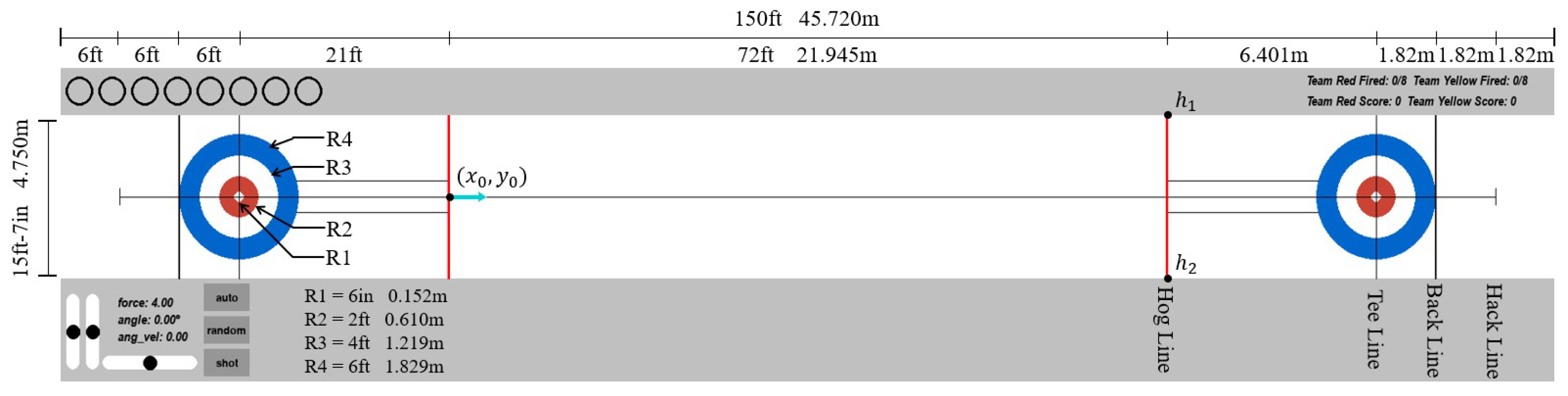
To train the RL agent effectively, we developed a full-scale custom curling simulator designed for stability, reproducibility, and efficient experimentation rather than perfect physical replication (Figure 1). The simulator follows the geometric layout and core rules defined by the World Curling Federation (WCF), including essential gameplay constraints such as the five-rock free guard zone (FGZ) rule, and provides automatic scoring for end-level evaluation. Several low-level physical effects are simplified to ensure consistent training dynamics and computational efficiency, reflecting the modeling choices commonly made in prior curling simulators.
Prior curling simulators were often designed around specific study objectives and modeling choices. Oberlin reports [16] using a Python-based simulator developed by Brunner (implemented with pygame and pymunk) and adapting it to generate training samples; the implementation includes pragmatic simplifications such as ignoring the magnitude of a rock’s angular velocity and injecting action noise to emulate execution imprecision. Silva et al. [17] employ the curling simulator of Yee et al. [11], which was designed to reflect execution uncertainty calibrated from Olympic statistics; sweeping is not modeled explicitly, and its effect is instead captured through an uncertainty model based on a heavy-tailed Student-t distribution. In contrast, our simulator is implemented as a general-purpose backend for unified DRL strategy learning, emphasizing stable and reproducible rollouts and end-level evaluation under the rules considered in this work.
The environment provides the agent with continuous control over three primary shot parameters (release force, angle, and spin), allowing it to explore a wide range of possible shots without being constrained by discrete predefined actions. Instead of reproducing exact physical interactions, the simulator focuses on preserving relative consistency among trajectories (e.g., faster throws travel farther; clockwise spins curl rightward) so that the agent can meaningfully associate actions with outcomes.
The motion of a curling stone is primarily influenced by its initial release conditions and the gradual deceleration caused by ice friction. Instead of modeling the full fluid–solid interactions that occur on real ice, our simulator employs an empirical, velocity-dependent friction model that captures the essential slowing behavior observed in curling. The frictional coefficient decreases slightly at higher speeds and increases as the stone slows, which qualitatively reproduces the stone’s curved trajectory near the end of its motion.
In addition to translational deceleration, a small asymmetric friction component is applied based on the stone’s rotational direction. This asymmetry induces gentle lateral displacement, representing the curving behavior characteristic of real curling shots. The magnitude of this effect is calibrated empirically to produce consistent curling behavior without introducing numerical instability.
All parameters, including mass, friction coefficients, and restitution constants, were tuned to maintain smooth simulation dynamics across thousands of episodes. The objective of this modeling is not to reproduce physical accuracy but to provide a coherent and stable mapping between action parameters and resulting trajectories, allowing reinforcement learning algorithms to focus on strategy optimization and policy convergence. Further refinement of the physical model, such as incorporating sweeping mechanics or stochastic ice variations, is left for future work as it lies beyond the primary scope of reinforcement learning-based strategy discovery.
A detailed description of the simulator implementation and the video-based calibration is provided in Appendix A.

2.2. Learning Curling Agents

To train the curling agent using reinforcement learning, we define the Markov Decision Process (MDP) as M = ( S , A , T , R , γ ) , where S represents the state space, A the action space, T the transition dynamics, R the reward function, and γ the discount factor. Since our approach is model-free, we do not explicitly model T but instead learn from sampled transitions. In this work, one RL episode corresponds to one end. The time step t indexes the shot order within the end, and the horizon is 16 deliveries (8 per team) under alternating turns in self-play. The episode terminates after the final delivery once all stones come to rest and the end score is computed.

2.2.1. State s

The state s t S at time step t consists of three components. The spatial component s t pos captures the positions and basic attributes of all stones on the ice, providing essential geometric information for evaluating possible shot outcomes. The contextual component s t ctx encodes turn-related information, including the current shot order, enabling the agent to plan strategically across the progression of an end. The game-level component s t game represents the relative score context, allowing the agent to adjust its decision-making between offensive and defensive strategies. Combined, these components constitute a structured state representation in s t = { s t pos , s t ctx , s t game } R 16 × 5 , formed by concatenating s t pos , s t ctx , and s t game along the column dimension, where each row corresponds to a stone and each column encodes spatial or contextual attributes relevant to curling strategy.
The stone-related component s t pos describes the spatial configuration and team identity of all stones on the sheet at time step t. Each stone is represented by a three-dimensional vector ( x i , y i , τ i ) , where x i and y i indicate the planar coordinates of the stone, and τ i { 0 , 1 } denotes its team. To improve numerical stability and make the learning invariant to the physical units of the sheet, we normalize all stone positions by the sheet dimensions. Let x min , x max , and y min , y max be horizontal and vertical boundaries of the playable area. The coordinates ( x i , y i ) are normalized as
x i x i x min x max x min , y i y i y min y max y min ,
so that x i , y i [ 0 , 1 ] for any stone inside the sheet. Stones that have not been thrown yet or have left the sheet are encoded as ( x i , y i , τ i ) = ( 1 , 1 , 1 ) to distinguish them from valid normalized positions. The complete stone state is defined as a fixed 16 × 3 structure, which corresponds to the maximum number of stones that can appear during an end.
The contextual component s t ctx encodes the shot-order information at time step t. It is represented as a one-hot vector of size 16 × 1 , where each entry t i corresponds to the i-th shot position for i = 1 , , 16 . The value t i = 1 indicates that the current turn is associated with the i-th shot, while all remaining entries are set to zero. This representation enables the agent to understand the progression within an end and to adjust its strategic decisions as the shot sequence advances. Early turns often involve guard placement or setup plays, whereas later turns typically focus on scoring attempts or takeouts. The fixed-length encoding ensures consistent contextual information throughout training and evaluation.
The game-related component s t game captures the relative score at time step t based on the current house configuration. The score is computed from the perspective of the agent’s team, which is fixed as the Red team. A positive value indicates that the agent’s team is currently leading, whereas a negative value indicates that the opponent is ahead. To maintain consistency with the dimensionality of the other state components, the scalar score is expanded into a 16 × 1 structure by repeating the same value across all entries. This design ensures that the score information aligns with the fixed-size state representation used for learning, while providing the agent with an interpretable indicator of the game’s strategic context.

2.2.2. Action a

At time step t, the agent produces a normalized action a ^ t = ( F ^ t , θ ^ t , ψ ^ t ) [ 1 , 1 ] 3 , which is mapped to the physical control variables a t = ( F t , θ t , ψ t ) used by the simulator. The physical ranges are F [ 0 , 8 ] , θ [ θ min , θ max ] , and ψ [ 1.5 , 1.5 ] . We use the affine mapping
F t = 0 + F ^ t + 1 2 × 8 , θ t = θ min + θ ^ t + 1 2 ( θ max θ min ) , ψ t = ψ ^ t × 1.5
here, F denotes the release force, θ the release angle, and ψ the angular velocity.
The bounds for the release angle are determined by the sheet geometry shown in Figure 1. Let ( x 0 , y 0 ) be the initial stone position, and let h 1 = ( x h , y h max ) and h 2 = ( x h , y h min ) denote the upper and lower endpoints of the admissible target region on the hog line. The angle toward a point ( x , y ) is
θ ( x , y ) = tan 1 y y 0 x x 0 ,
yielding the feasible range
θ min = tan 1 y h min y 0 x h x 0 , θ max = tan 1 y h max y 0 x h x 0 .
These bounds ensure that the release direction points toward permissible regions of the sheet.
Actions are selected by a stochastic policy parameterized in the normalized space. The actor outputs μ ϕ ( s t ) and log σ ϕ ( s t ) for a Gaussian distribution over a pre-squash variable u t R 3 :
ϵ t N ( 0 , I ) , u t = μ ϕ ( s t ) + σ ϕ ( s t ) ϵ t , a ^ t = tanh ( u t ) , a t = ( F t , θ t , ψ t ) ,
where ⊙ denotes element-wise multiplication and ( F t , θ t , ψ t ) is obtained from a ^ t via the affine mapping above. During evaluation, we sample actions from the Gaussian policy parameterized by μ ϕ ( s t ) and σ ϕ ( s t ) , rather than using the mean action.

2.2.3. Reward r

The reward function r ( s t , a t ) is designed to guide the agent toward accurate shot execution and strategic gameplay within a curling end. It consists of three components that jointly capture shot quality, rule-valid placement, and strategic impact on scoring.
The first component evaluates shot precision by measuring the stone’s final distance from the tee. This term encourages the agent to generate valid curling shots that land closer to the house. The distance-based reward is computed as
R dist = ( x t x T ) 2 + ( y t y T ) 2 ( x 0 x T ) 2 + ( y 0 y T ) 2 ,
where ( x t , y t ) denotes the stone’s landing position and ( x T , y T ) is the tee at the center of the house. By normalizing the final distance with respect to the initial distance, this formulation encourages progressive improvements in shot accuracy.
To ensure that learning progresses within meaningful game states, an auxiliary placement reward promotes keeping the stone inside the playable area. This term is defined as
R area = 0.15 , x min x t x max and y min y t y max , 0 , otherwise ,
where x min , x max denote the longitudinal boundaries between the hog line and the back line, and y min , y max represent the lateral rink boundaries. This reward prevents convergence to degenerate actions that launch stones outside the sheet. The constant 0.15 in R area was selected via preliminary tuning to provide a mild shaping signal that penalizes out-of-sheet outcomes without overriding the score-based objective. The effect of R area on reducing out-of-sheet outcomes is examined in a limited sensitivity test (see Section 3.3).
The third component captures the strategic value of a shot by evaluating how the scoring advantage shifts as a consequence of the current stone placement. Rather than using the absolute score differential, the reward is defined based on the incremental gain achieved by the current action relative to the previous state. Let A denote the learning agent’s team (corresponding to the red stones), and O denote the opponent’s team (corresponding to the yellow stones). Formally,
R score = λ t ( score t A score t O ) ( score t 1 A score t 1 O ) , if t > 0 , λ t ( score t A score t O ) , otherwise .
The weighting coefficient λ t increases for later shots within an end to reflect their higher strategic impact:
λ t = 1.0 , if the shot is the final delivery , 0.5 , otherwise .
We use a simple binary schedule for λ t to stabilize score-based shaping during the end. Early and intermediate shots often serve as positional setup, where the instantaneous house score can be volatile; thus we set λ t = 0.5 for non-final deliveries. For the final delivery, we set λ t = 1.0 to fully reflect its direct impact on the end outcome. In addition to these three reward components, the environment also enforces the FGZ rule. Any shot that violates this rule receives a fixed penalty of 1 . Although this penalty is not explicitly included in the mathematical formulation above, it is applied during training to ensure adherence to official gameplay regulations.
The overall reward is expressed as the sum of these three components:
r ( s t , a t ) = ( 1 p ) R dist + p ( R area + R score ) .
Here, p = 0 corresponds to Phase 1 (placement-only learning), and p = 1 corresponds to Phase 2 (strategic self-play), allowing the same MDP structure to be used while the reward focus is switched between phases. For simplicity and reproducibility, we adopt a fixed curriculum schedule: we train Phase 1 for 2000 episodes and then switch to Phase 2. This formulation jointly encourages accurate shot placement, adherence to valid gameplay regions, and strategically meaningful decisions throughout the end. From the MDP perspective, we treat the completion of an end (i.e., after the final delivery and once all stones come to rest and scoring is evaluated) as a terminal transition. A new end starts with an environment reset and is modeled as a new episode.

2.2.4. Soft Actor–Critic for Deep Reinforcement Learning

Continuous control is essential for curling because a shot is determined by continuous-valued delivery parameters such as force, angle, and angular velocity. Moreover, the effectiveness of a shot depends on future strategic possibilities including guard placement, promotion, and scoring potential. These characteristics require an RL algorithm capable of exploring a continuous action space while maintaining stability under stochastic dynamics. For these reasons, we employ the Soft Actor–Critic (SAC) algorithm [18], which provides entropy-regularized policy optimization and high sample efficiency through its off-policy learning paradigm.
Given the curling MDP, the soft Q-function is defined as
Q ( s t , a t ) = r ( s t , a t ) + γ E s t + 1 p ( · | s t , a t ) V ( s t + 1 ) ,
where the reward function r ( s t , a t ) is the composite curling reward introduced in Section 2.2.3.
The soft value function incorporates entropy regularization:
V ( s t ) = E a t π ϕ ( · | s t ) Q ( s t , a t ) α log π ϕ ( a t s t ) ,
where α is the temperature controlling the trade-off between exploration and exploitation.
Our SAC employs double Q-networks and the Soft Bellman backup:
y t = r ( s t , a t ) + γ E a t + 1 π ϕ min i = 1 , 2 Q θ i ( s t + 1 , a t + 1 ) α log π ϕ ( a t + 1 s t + 1 ) .
The policy is parameterized in the normalized action space (Section 2.2.2) and optimized using
J π ( ϕ ) = E s t D E a t π ϕ α log π ϕ ( a t s t ) Q ( s t , a t ) .
The entropy coefficient is learned automatically with
J ( α ) = E a t π ϕ α log π ϕ ( a t s t ) + H ,
where H is a target entropy chosen according to the dimensionality of the continuous action space. By integrating SAC into the proposed curling MDP, the agent learns diverse and robust strategies while maintaining training stability under continuous control. Both the policy and value functions are approximated by simple deep neural networks.
The policy network π ϕ and the two soft Q-functions Q θ 1 and Q θ 2 are implemented using multilayer perceptron (MLP) architectures. The actor network receives the flattened state s t (defined in Section 2.2.1) as input and processes it through two fully connected hidden layers of dimension 256 with ReLU activation. The output layer simultaneously produces the mean vector μ ϕ ( s t ) and the log-standard-deviation vector log σ ϕ ( s t ) for the Gaussian distribution of the pre-squash variable u t R 3 . For numerical stability, each entry of log σ ( s t ) is clipped to the interval [ 5 , 2 ] , after which exponentiation is applied to obtain the standard deviation σ ( s t ) . These parameters define a Gaussian policy, and the sampled action is passed through a hyperbolic tangent transformation to ensure that all components lie within the normalized range [ 1 , 1 ] . The resulting normalized action in then affinely rescaled to the physical ranges of ( F t , θ t , ψ t ) , as described in Section 2.2.2.
The critic networks employ the same MLP structure as the actor (two fully connected layers of width 256 and ReLU activations) but end with a single linear output neuron that estimates the state–action value Q θ i ( s t , a t ) . Although the two Q-networks share the same architecture, their parameters are initialized independently to construct the twin-Q structure of SAC. To improve training stability, all fully connected layers use orthogonal weight initialization, and biases are initialized to zero.

2.2.5. Two-Phase Learning Strategy

To train competitive curling agents, we adopt a two-phase curriculum learning strategy followed by a self-play framework. The central motivation is to decouple low-level shot acquisition from high-level strategic reasoning, thereby stabilizing exploration in the continuous action space. In Phase 1, the agent is trained in a single-agent setting to master fundamental delivery mechanics. Reward shaping focuses solely on locating the stone near the tee line ( R dist ), encouraging the agent to learn reliable release force, angle, and spin control without exposure to adversarial interaction. This stage provides a robust foundation for precise shot execution, mitigating the severe optimization difficulty that arises when strategic and physical learning are entangled from the outset.
To compactly express the two-stage curriculum, we introduce a phase indicator p { 0 , 1 } in the reward function in Section 2.2.3 that switches the objective between low-level shot acquisition and strategic scoring. During Phase 1 ( p = 0 ), the agent is trained solely to master delivery mechanics around the tee line using only the distance-based term R dist . In Phase 2 ( p = 1 ), the objective shifts to strategic play, where the agent is rewarded for creating advantageous house configurations through the area- and score-based terms R area and R score .
Once the agent demonstrates stable placement behavior, training transitions to Phase 2, where strategic learning is introduced through self-play. Two agents are instantiated: a learning agent (Red Team) and a fixed opponent (Yellow Team), both initialized from the Phase 1 policy. Unlike Phase 1, the reward function expands to include the score-based component, enabling the agent to reason about game context, offensive opportunities, and defensive maneuvers across an entire end.
To ensure stable adaptation during early competitive learning, we employ a win-rate-based opponent update mechanism. The Yellow Team serves as a frozen snapshot of a previously learned policy, while the Red Team continues to update its parameters via Soft Actor–Critic (SAC). Whenever the Red Team achieves a predefined win-rate threshold against the current Yellow Team, the opponent’s parameters are synchronized to those of the learner. This gradual opponent escalation produces a performance-driven curriculum, allowing the agent to encounter progressively stronger adversaries without abrupt shifts in opponent behavior or policy collapse. The overall Phase 2 training procedure is summarized in Algorithm 1.
Algorithm 1 Self-Play Training Process
1:Initialize Red Team (learning agent) and Yellow Team (fixed opponent)
2:Set initial policy parameters ϕ Red , ϕ Yellow ϕ Red
3:Initialize replay buffer D
4:for each episode do
5:      Initialize environment and observe initial state s 0
6:      for each shot index t in the end ( t = 1 , , 16 ) do
7:            Determine acting team c ( t ) from the shot order (alternating turns)
8:            if  c ( t ) = RED  then
9:                  a t π ϕ Red ( · s t )
10:            else
11:                  a t π ϕ Yellow ( · s t )
12:            end if
13:            Execute action and transition s t + 1 p ( · s t , a t )
14:            if  c ( t ) = RED  then
15:                 Compute reward r t = r ( s t , a t )        ▹ Red team’s perspective
16:                 Store transition D D { ( s t , a t , r t , s t + 1 ) }
17:            end if
18:      end for
19:      for each gradient update step do
20:            Update ϕ Red using SAC with replay buffer D
21:            if win_rate ( ϕ Red ) threshold  then
22:                  ϕ Yellow ϕ Red               ▹ policy synchronization
23:            end if
24:      end for
25:end for

3. Experiments and Results

In this section, we present a comprehensive experimental evaluation of the proposed unified reinforcement learning framework for strategic curling. Our goal is to verify that the proposed simulator and MDP design and two-phase curriculum enable stable long-horizon learning under continuous shot control, and to quantify how effectively the resulting policies translate mechanical shot execution into end-level strategic advantage. To this end, we conduct controlled experiments under consistent training and evaluation protocols, emphasizing fairness across algorithms and reproducibility of all reported results.
We begin by summarizing reproducibility details, including the exact code reference and the principal training configurations used throughout the study (Section 3.1). Next, we evaluate learning dynamics and competitive strength by benchmarking representative continuous-control RL methods under identical conditions, using both learning curves and head-to-head match outcomes as primary evidence (Section 3.2). We then isolate the contribution of key MDP components via ablation studies, analyzing how game-context signals, score-based shaping, and rotational control affect performance and behavior (Section 3.3). Finally, we assess whether the learned agent exhibits tactically plausible patterns by qualitatively comparing selected agent decisions with situations observed in elite curling match records, providing an interpretable link between simulated self-play strategies and real-world competitive play (Section 3.4).

3.1. Reproducibility Details

To ensure full reproducibility of the reported results, we provide an immutable reference to the exact codebase and experimental settings used in this study. The complete simulator and training pipeline, including training scripts and evaluation utilities, are publicly available at https://github.com/son-yu-seoung/Reinforcement-Learning-for-Discovering-Curling-Strategies-Using-a-Custom-Simulator (accessed on 5 November 2025). In addition, we provide a versioned release tag (v1.0.0) that uniquely identifies the precise code snapshot corresponding to this manuscript.
All experiments were conducted with fixed random seeds under identical architectural settings across SAC, A2C, and PPO. Table 1 summarizes the principal experimental configurations, including key hyperparameters and optimizer settings for each algorithm, together with the hardware and software specifications used for all runs. Using this fixed setup, we next evaluate both learning dynamics and competitive performance of the trained agents.

3.2. Evaluating RL Agents for Curling

To evaluate the effectiveness of the proposed curling RL framework, we conducted a series of experiments focusing on both quantitative and qualitative aspects of agent behavior. Our primary objective was to determine whether the proposed MDP design and the two-phase curriculum enable stable learning across different reinforcement learning algorithms.
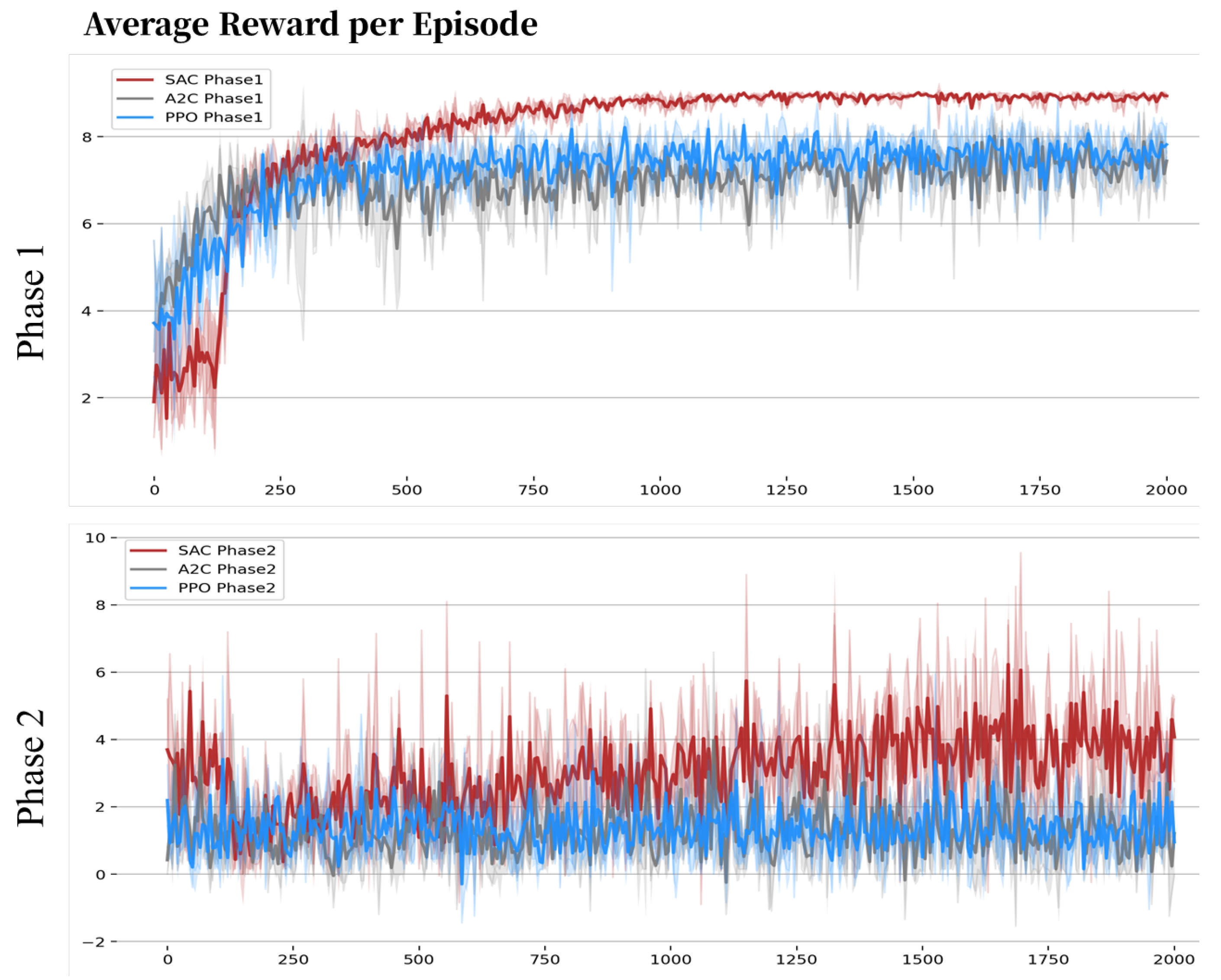
We benchmarked three representative continuous-control methods, Soft Actor–Critic (SAC), Proximal Policy Optimization (PPO), and Advantage Actor–Critic (A2C) under identical simulator conditions and architectural settings. As shown in Figure 2, during Phase 1, where only the distance-based reward is active, all agents progressively learn basic delivery mechanics. However, SAC demonstrates markedly faster convergence and reaches a substantially higher asymptotic reward than both PPO and A2C, indicating superior stability and sample efficiency in the early stage of curling skill acquisition.
The difference between algorithms becomes more pronounced in Phase 2, where the reward function transitions to the area- and score-based terms and agents enter competitive self-play. This setting introduces sparse and delayed returns, substantially increasing the difficulty of policy optimization. Under this regime, SAC continues to steadily improve and maintains stable reward progression, whereas PPO and A2C exhibit oscillatory or stagnant behavior despite extended training. These results suggest that entropy-regularized off-policy learning is particularly advantageous in curling, where continuous shot parameters and strategic game outcomes must be jointly optimized. Overall, SAC proves to be the most robust approach across both phases, successfully transferring low-level mechanical skill into high-level strategic decision-making.
Beyond the learning curves, we assess the competitive strength of the trained agents via direct head-to-head evaluation. In our experiments, each match begins with the Red team throwing first, and the teams alternate the first throw from match to match. Hammer possession within an end follows the standard curling rule: the team that does not score in an end receives the hammer in the subsequent end. In a blank end (i.e., an end in which neither team scores), the hammer is retained by the same team for the next end. As summarized in Table 2, each pairing is tested over 30 matches, where each match consists of 10 ends and the random seed is resampled per match; we report both the match-level outcome (Win–Draw–Loss from the Red team’s perspective) and the averaged score differential (Score Avg and End Score Avg).
In the Phase 2 vs. Phase 2 setting, the SAC agent exhibits the strongest overall performance. Against A2C, SAC achieves a 24–0–6 record and attains a high average score (Score Avg: 11.43 ± 4.07 ). In contrast, A2C shows a lower average score (Score Avg: 4.93 ± 2.72 ). Against PPO, SAC achieves a perfect 30–0–0 record and the largest margin (Score Avg: 16.37 ± 3.83 ). These results suggest that the combination of off-policy learning with strategic reward terms and entropy regularization enables SAC to discover advantageous shot patterns and reliably convert them into scoring outcomes. In addition, the A2C–PPO matchup indicates that A2C is comparatively weaker, recording 11–0–19, along with a lower average score.
The benefits of the proposed two-phase training strategy become more evident in Phase 2 vs. Phase 1 comparisons. SAC consistently outperforms all Phase 1 agents trained only for placement, showing particularly large gaps against A2C and PPO with records of 27–0–3 and 27–0–3, respectively. In some matches, Phase 1 agents occasionally secure wins; this can be attributed to their lack of contextual reasoning, which often leads them to take overly aggressive or poorly positioned shots that inadvertently create scoring opportunities. In contrast, the Phase 2 SAC adapts its behavior to the shot context and leverages freezes, guards, and come-around trajectories to establish multi-stone scoring positions. Overall, these findings highlight that the transition from mechanical skill acquisition (Phase 1) to strategic optimization (Phase 2) is crucial for curling performance, and that SAC can effectively exploit this transition to achieve strong competitive strength.

3.3. Ablation Studies

Among the components of the MDP M , the game-context information s t game and the score-based reward R score are crucial for strategic decision-making. Curling does not reward purely high-precision placements; agents must evaluate advantageous house configurations, deny scoring opportunities to the opponent, and adapt shot selection accordingly. Without game-context feedback, the agent tends to optimize local stone placement but fails to reason about global scoring outcomes, resulting in limited offensive or defensive intent.
Angular velocity ψ is another essential factor for tactical diversity. Removing curl forces the agent to rely solely on linear force F and release angle θ , which restricts its ability to execute core curling maneuvers such as guards, freezes, or come-arounds that require curved trajectories. Prior approaches often fix spin direction to a discrete set or eliminate rotation entirely [8,19,20], thus reducing the expressive capacity of the action space. In contrast, our formulation treats ψ as a continuous control variable, allowing for wider behavioral variation in the house.
Table 3 reports head-to-head results for the proposed agent and its ablated variants. The full model consistently dominates the ablations, showing the strongest win–draw–loss records and the largest average score margins. When we remove the game-context signals ( s t game ) and the score-based reward term ( R score ) , performance drops substantially, indicating that strategic awareness is critical for end-level decision-making. Disabling curl by fixing angular velocity ( ψ = 0 ) also causes a clear degradation: while the agent can still place stones near the house, it becomes less effective at executing tactically important curved trajectories (e.g., guards, freezes, and come-arounds), particularly against defensive responses. The most restricted variant that removes both game-context and curl performs worst overall, confirming that game-context shaping and rotational control provide complementary benefits for competitive curling play.
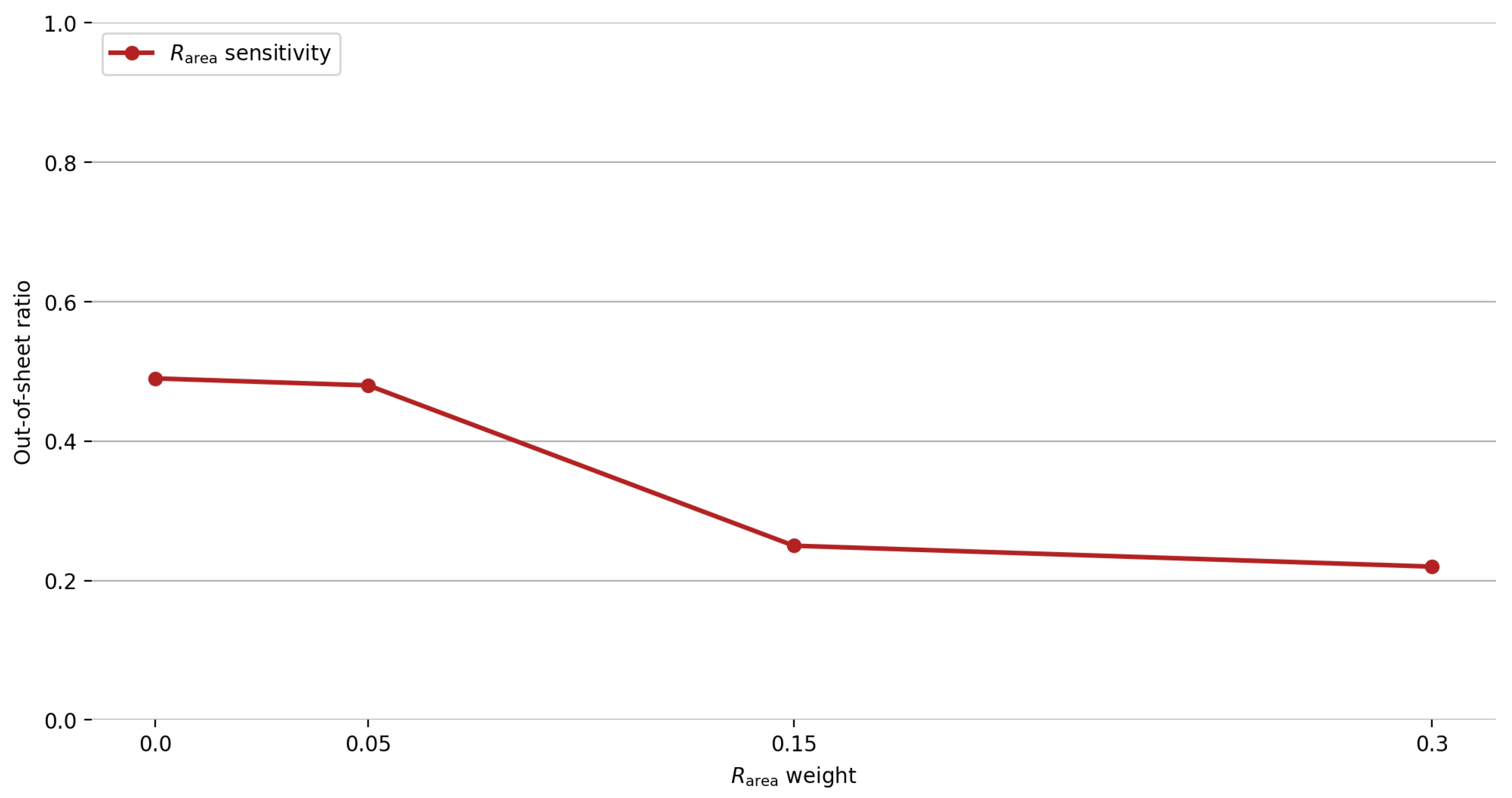
To verify that the auxiliary placement term R area functions as intended, we conduct a limited sensitivity test by varying only the weight of R area while keeping all other components of the reward and the training protocol unchanged. We report the out-of-sheet ratio, defined as the fraction of executed shots whose final stone state lies outside the playable sheet boundary. As shown in Figure 3, increasing the weight of R area lowers the out-of-sheet ratio, from about 0.5 at weights 0– 0.05 to about 0.22 at 0.3, confirming that this term provides an effective shaping signal to discourage degenerate actions that immediately exit the sheet.
Importantly, a non-zero out-of-sheet ratio is expected even under well-executed play, because this metric also counts strategically valid take-out outcomes in which the stone (or the contacted opponent stone) leaves the playing area after collision. The nonzero out-of-sheet rate at higher weights (≈0.2) is expected, since it includes both intentional take-outs and occasional exits after high-impact collisions, rather than indicating persistent execution failure.

3.4. Comparison Between the AI Agent and an Elite Curling Team

To qualitatively examine whether the AI agent’s decisions exhibit tactical patterns similar to those seen in elite curling matches, we utilized the game record data from the men’s division of the Le Gruyère AOP European Curling Championships 2023, organized by the World Curling Federation [21]. The dataset consists of a PDF file spanning a total of 500 pages, which is accessible on the website. From these pages, a total of 6512 shot images were extracted, and stone position data were automatically retrieved using the Hough Circle Transform combined with image processing techniques. To map the detected stone-center coordinates to the simulator’s sheet coordinate system, we compute two independent scaling factors. (i) The longitudinal scale ratio, s x , is defined as the ratio between the hog-to-back line distance measured in the image and the corresponding physical distance used in the simulator. (ii) The lateral scale ratio, s y , is defined as the ratio between the sheet width in the image and the sheet width in the simulator. Each detected stone center is expressed in tee-centered relative coordinates. The longitudinal component is scaled by s x , and the lateral component is scaled by s y . The scaled coordinates are then transformed into the simulator’s coordinate frame. Because the broadcast charts are generated from a consistent template, the calibration of the hog and back lines, as well as that of the sheet boundaries, is performed once and reused for all frames, which ensures consistent alignment across the entire dataset.
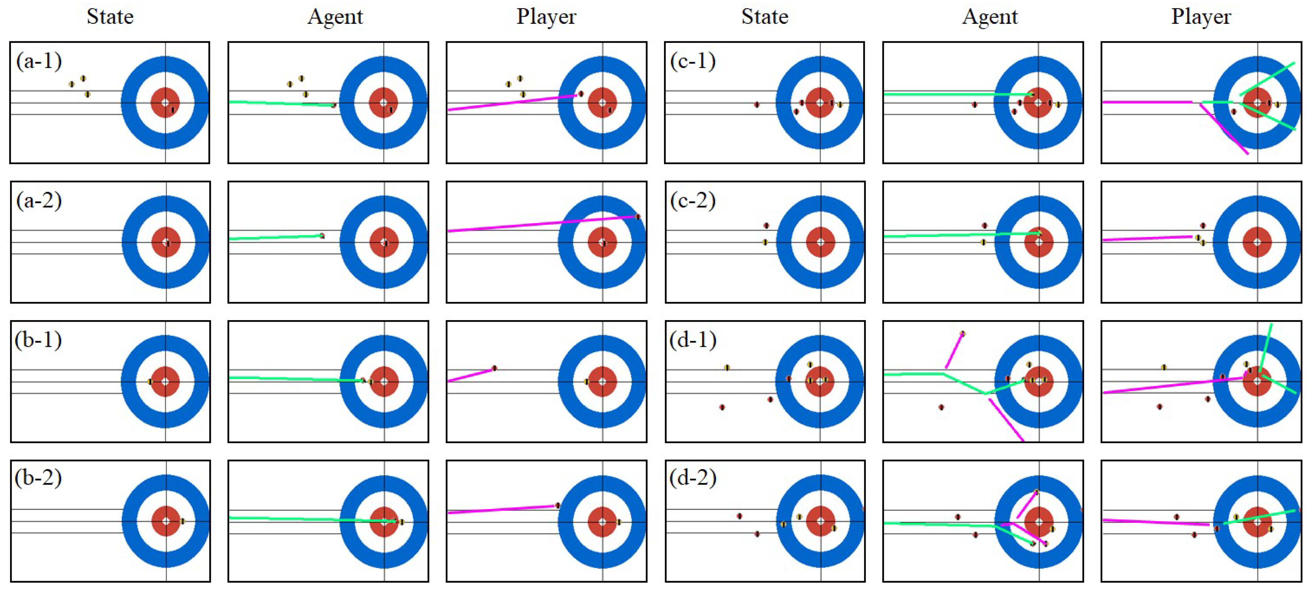
However, Figure 4 presents a qualitative case study based on a selected subset of representative situations, rather than all extracted shots. Specifically, we analyze outcomes from Guard, Freeze, Come-around, and Hit & Roll shots to probe the agent’s strategic inference across typical, defensive, and offensive contexts. By comparing the agent’s decisions with those observed in elite match play, we assess the extent to which the learned strategies align with professional behavior and highlight key differences.
In the first scenario Figure 4(a-1,a-2), the agent executed a shot that left the stone short, positioned in front of the house. This placement forced the opponent to make a direct removal attempt while securing a defensive position with minimal risk. This shot type is classified as a Guard in curling. In the second scenario Figure 4(b-1,b-2), the agent positioned the stone in a location where it could not be immediately taken out by the opponent, effectively limiting the opponent’s strategic options. This shot corresponds to a Freeze, a highly effective technique that can exert psychological pressure on the opposing team.
In scenario Figure 4(c-1,c-2), the agent considered a Come-around shot. In Figure 4(c-1), it navigated past the opponent’s guard and directly secured a scoring position in a complex house setup. In Figure 4(c-2), it skillfully passed between two stones, naturally utilizing the opponent’s stones as guards. Additionally, in scenario Figure 4(d-1,d-2), the agent executed a Hit & Roll strategy, where it not only took out the opponent’s stone but also repositioned its own stone into a more advantageous location. This is a highly advanced technique, often leading to errors among even professional players. The fact that the agent was able to learn and apply such a high-level technique without explicit guidance suggests that it can exhibit tactically plausible behaviors that resemble patterns observed in expert match play in selected examples.
The agent demonstrated proficiency in executing a variety of shot types, including Guard, Freeze, Come-around, and Hit & Roll. These examples indicate that the AI agent can execute a variety of recognizable shot patterns and adapt its decisions to different in-end situations in our simulator.

4. Discussion and Conclusions

In this work, we introduced a unified reinforcement learning framework for curling that integrates a physically grounded simulator, a curling-specific MDP formulation, and a two-phase training strategy. Unlike previous approaches that rely on discrete shot candidates or handcrafted decision rules, our framework enables agents to directly control continuous delivery parameters (release force, angle, and spin) while reasoning over evolving strategic contexts within an end. Experimental results demonstrate that this design yields stable training dynamics, human-like tactical behavior, and competitive superiority over ablated variants and alternative RL baselines.
A central finding of this study is the importance of curriculum structure in long-horizon physical sports. During Phase 1, agents learned delivery consistency under distance-only objectives, forming a foundation of reliable shot mechanics. Transitioning to Phase 2 introduced adversarial self-play and score-based rewards, enabling agents to develop both offensive and defensive strategic reasoning. As shown in the learning curves (Figure 2) and head-to-head evaluations (Table 2), SAC transferred placement proficiency into multi-stone scoring strategies, while PPO and A2C stagnated or oscillated under sparse and delayed rewards. These observations highlight that entropy-regularized off-policy learning is particularly advantageous in curling, where exploration in continuous action space must coexist with context-dependent decision-making.
The ablation results further clarify which MDP components contribute to high-level curling competence. Removing relative score context and its associated reward diminished strategic awareness, hence agents could place stones well but failed to deny opponent scoring or maintain favorable house configurations. Eliminating angular velocity constrained maneuverability and suppressed core curling patterns such as come-around and freeze. The worst-performing variant removed both, reducing the game to mechanical placement without tactical foresight (Table 3). These outcomes indicate that curling strategy emerges not merely from accuracy, but from the interaction of game-context signals and rotational control, which collectively support nuanced shot selection.
Beyond quantitative metrics, qualitative evaluations revealed that the agent autonomously discovered hallmark curling strategies, including guard, freeze, come-around, and hit-and-roll plays. These behaviors were not explicitly encoded; rather, they emerged during self-play under the proposed MDP and simulator dynamics. This suggests that reinforcement learning can model higher-order dynamic reasoning in precision sports, bridging mechanical execution and situational tactics without handcrafted heuristics.
Despite these strengths, our framework inherits several limitations. First, the simulator excludes sweeping mechanics and advanced ice variability, both of which affect real-world shot outcomes. Second, Phase 2 relies solely on self-play; while this fosters robust competitive policies, it may bias learning toward equilibrium strategies that differ from human conventions. Third, the reward shaping components use empirical scaling, which may require adaptation under different rule sets or competition formats. Addressing these limitations constitutes meaningful avenues for future work. Integrating supervised imitation from elite match data, modeling stochastic ice conditions, and incorporating sweeping as a controllable variable may further improve realism, generalization, and strategic depth.
Overall, this study demonstrates that a carefully designed reinforcement learning framework can acquire professional-level curling tactics from first principles. By combining structured state representation, continuous shot control, and staged training, our approach moves beyond simulation accuracy or isolated strategy heuristics and toward holistic curling intelligence. We anticipate that this methodology will support future research in sports analytics, strategic AI, and agent-based coaching tools for real-world curling applications.


Author Contributions

Conceptualization, Y.S.; Methodology, Y.S. and B.J.; Software, Y.S.; Validation, B.J.; Formal analysis, B.J.; Investigation, Y.S.; Data curation, J.P.; Writing—original draft, Y.S.; Writing—review and editing, B.J.; Visualization, Y.S.; Supervision, B.J.; Project administration, Y.S., J.P. and B.J.; Funding acquisition, J.P. All authors have read and agreed to the published version of the manuscript.

Funding

This research was supported by the Culture, Sports and Tourism R&D Program through the Korea Creative Content Agency grant funded by the Ministry of Culture, Sports and Tourism in 2025 (Project Name: Development of smart curling strategy coaching technology based on intelligent motion coaching analysis, Project Number: RS-2023-00227655, Contribution Rate: 100%); and in part by the Hankuk University of Foreign Studies Research Fund, in 2026.

Institutional Review Board Statement

Not applicable.

Informed Consent Statement

Not applicable.

Data Availability Statement

The data used in this study consist of experience data collected during the training process. For reproducibility, we have publicly released the complete simulator and training pipeline, including the source code, configuration files, and scripts, at https://github.com/son-yu-seoung/Reinforcement-Learning-for-Discovering-Curling-Strategies-Using-a-Custom-Simulator (accessed on 5 November 2025).

Conflicts of Interest

The authors declare no conflict of interest.

Appendix A. Detailed Physical Modeling of the Simulator

This appendix describes the detailed physical equations used in the curling simulator. The equations include velocity-dependent frictional deceleration, asymmetric friction-induced curl bias, and inelastic collision handling.

Appendix A.1. Curling Simulator

The simulator follows the geometric layout and the fundamental rules of curling as defined by the World Curling Federation [22]. Figure 1 summarizes the full sheet dimensions implemented in the environment. To support realistic gameplay flow, the FGZ rule and standard scoring procedures are implemented. A lightweight user interface provides real-time score updates. The full implementation is available on GitHub: https://github.com/son-yu-seoung/Reinforcement-Learning-for-Discovering-Curling-Strategies-Using-a-Custom-Simulator (accessed on 5 November 2025).
  • Five-rock free guard zone (FGZ) rule implementation
We enforce the FGZ rule by evaluating violations after each delivery has fully settled. During the first five deliveries of an end, an opponent stone is treated as FGZ-protected if it lies between the hog line and the tee line and outside the house in the pre-shot state. A violation is triggered if any such protected opponent stone becomes out of play as a result of the shot. In that case, the delivered stone is removed and the affected opponent stone(s) are restored to their pre-shot positions. During training, the acting agent additionally receives a fixed penalty of −1.

Appendix A.2. Curling Stone Dynamics

We model the stone as a rigid body translating on a horizontal plane with a single scalar rotational velocity about the vertical axis. Let the stone’s state at time t be position x ( t ) = [ x ( t ) , y ( t ) ] , velocity v ( t ) = [ v x ( t ) , v y ( t ) ] , and spin ω ( t ) . The initial release is parameterized by the speed v 0 > 0 , heading angle θ ( π , π ] , and spin ω 0 :
v ( 0 ) = v 0 cos θ sin θ , ω ( 0 ) = ω 0 .
  • Velocity-Dependent Friction (Tangential Deceleration)
The dominant decelerating force is kinetic friction, whose effective coefficient decreases mildly at higher speeds and increases as the stone slows. We use the empirically motivated form
μ eff ( v ) = μ 0 + μ 1 e α v , v = v 2 ,
with constants μ 0 > 0 , μ 1 0 , and α 0 . The corresponding tangential acceleration is antiparallel to the velocity:
a ( v ) = μ eff ( v ) g v max ( v , ε ) ,
where g is gravitational acceleration and ε > 0 avoids division by zero near rest.
  • Asymmetric Friction-Induced Curl Bias (Lateral Drift)
Observed curling trajectories exhibit lateral drift whose direction depends on the spin. Instead of invoking an aerodynamic Magnus effect, we model this behavior as a small asymmetric friction component producing lateral acceleration perpendicular to v :
a ( v , ω ) = κ curl ω v R 90 v max ( v , ε ) ,
where κ curl 0 is a calibrated coefficient and R 90 ( [ a , b ] ) = [ b , a ] rotates a vector by + 90 . Positive ω yields rightward drift with respect to the heading direction, while negative ω yields leftward drift.
  • Spin Decay
Spin decays exponentially due to dissipative contact:
ω ˙ ( t ) = β ω ( t ) ω ( t ) = ω 0 e β t ,
with β 0 . In discrete time with step Δ t , we use ω k + 1 = ω k e β Δ t .
  • Time Integration (Semi-Implicit Euler)
For numerical stability over long rollouts, we integrate accelerations using a semi-implicit Euler scheme. Let a k = a ( v k ) + a ( v k , ω k ) , then
v k + 1 = v k + a k Δ t , x k + 1 = x k + v k + 1 Δ t .
To avoid spurious oscillations near rest, if v k + 1 2 < v min we set v k + 1 = 0 .
  • Numerical integration and sub-stepping
The simulator advances the dynamics using a fixed time step of Δ t = 5 × 10 4 s. Within a single rendered frame, the physics update is executed 20 times by default, i.e., each frame corresponds to 20 Δ t = 0.01 s of simulated time. In each discrete update, we first resolve inter-stone collisions and then advance all stones by one integration step.
  • Stopping criterion
To avoid numerical jitter near rest, if a stone’s speed satisfies v < v s t o p , we snap it to rest by setting v 0 and ω 0 . In the current implementation, v s t o p = 0.01 m/s. A shot is considered complete when all stones satisfy the rest condition; the update loop terminates early once all velocities are zero.
  • Inelastic Collisions
Let stones i and j have masses m i and m j , centers p i and p j , radii r i and r j , and pre-impact velocities v i and v j . A collision occurs if
p i p j 2 r i + r j .
Define the collision normal
n = p i p j max ( p i p j 2 , ε ) ,
and the relative normal speed v n = ( v i v j ) · n . With normal coefficient of restitution e n [ 0 , 1 ] , the impulse magnitude is
J = ( 1 + e n ) v n 1 m i + 1 m j .
The post-impact velocities are
v i = v i + J m i n , v j = v j J m j n .
For simplicity and robustness, we do not exchange tangential impulses or torques; instead, we apply a scalar spin damping factor on collision,
ω i = ρ ω i , ω j = ρ ω j , 0 < ρ 1 ,
which empirically captures the small loss of rotational energy without introducing instability from frictional torque estimation.
  • Physical Parameters
Table A1 lists the parameters used in the simulator. Values were tuned to produce qualitatively consistent trajectories and stable long-horizon rollouts suitable for reinforcement learning experiments.
Table A1. Physical parameters used in the curling simulator.
ParameterValueDescription
μ 0 0.020Baseline friction coefficient
μ 1 0.005Velocity-dependent friction term
α 0.050Decay rate in μ eff ( v )
κ curl 0.10Asymmetric friction coefficient
e n 0.92Normal restitution coefficient
ρ 0.95Spin damping factor after collision
m18.0 kgMass of the curling stone
g9.81 m/s2Gravitational acceleration
β 0.070Spin decay rate
I0.174 kg·m2Moment of inertia
v min 0.02 m/sVelocity threshold for stopping
ε 10 6 Small constant for numerical stability
All parameters were chosen to ensure stable dynamics and to produce qualitatively curling-like motion. Top-view match footage was additionally used as a reference to calibrate coarse behavioral patterns, such as typical travel distances and curl directions. We additionally report a quantitative trajectory-level validation against top-view match footage in Appendix A.3.
  • Remarks on Model Scope
Equations (A2)–(A11) define a coherent approximate model intended to provide a stable and reproducible mapping from actions to trajectories for reinforcement learning. High-fidelity effects such as sweeping, detailed ice texture variation, and frictional torque exchange during impacts are left to future extensions, as they are orthogonal to the present study’s focus on strategy learning.

Appendix A.3. Video-Based Calibration and Quantitative Validation

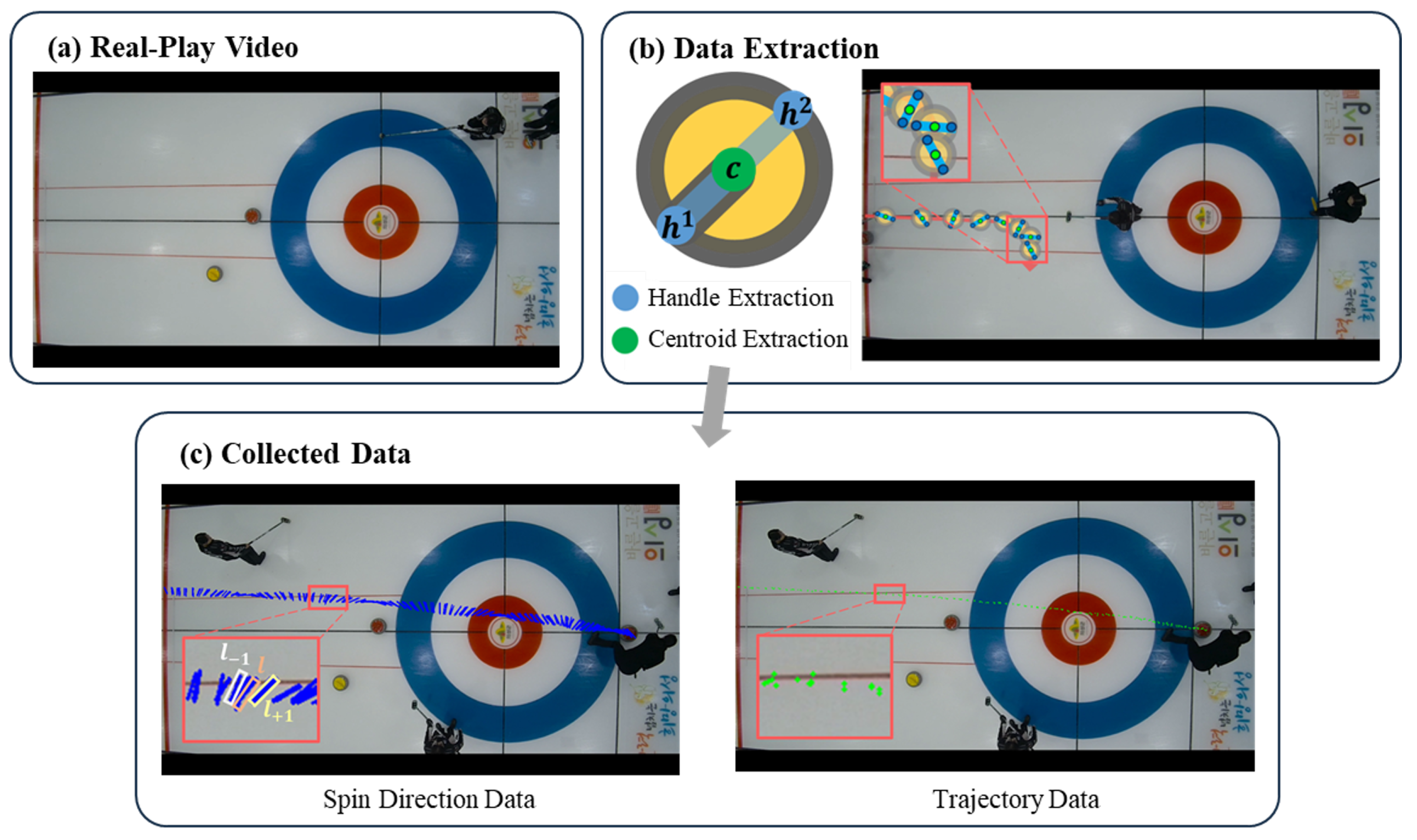
To provide reader-accessible quantitative evidence that the proposed simulator plausibly reproduces the dynamic motion of curling stones, we conducted a video-based calibration and validation using real match footage. The reference dataset consists of six top-view (planar-view) videos recorded at the Uiseong and PyeongChang curling rinks in South Korea. Each video has a resolution of 1280 × 720 at 30 fps. From a multi-camera setup installed to capture athletes’ training sessions from multiple viewpoints, we used the top-view camera (Figure A1a) for trajectory extraction and comparison.
Figure A1. Process of stone information extraction from real-play video for simulator calibration.
Mathematics 14 00403 g0a1
To reduce perspective distortion and focus on the physically meaningful segment, each clip was temporally trimmed from the moment the stone crosses the hog line to the moment the stone comes to rest. The raw videos have an average duration of 35 s, while the trimmed clips have an average duration of 9.67 s.
Specifically, to extract position and rotation information from the top-view footage, we manually annotated the stone center and the two endpoints of the handle in each frame (Figure A1b). The annotation was performed at 30 frames per second, resulting in 174–329 annotated frames per video depending on the shot duration. The resulting measurements were temporally aligned to compute trajectory errors. The quantitative comparison was performed within a Region of Interest (ROI), which corresponds to the critical zone where the stone’s curl and final placement are determined. We define the ROI as the segment from the hog line closest to the house to the back line.
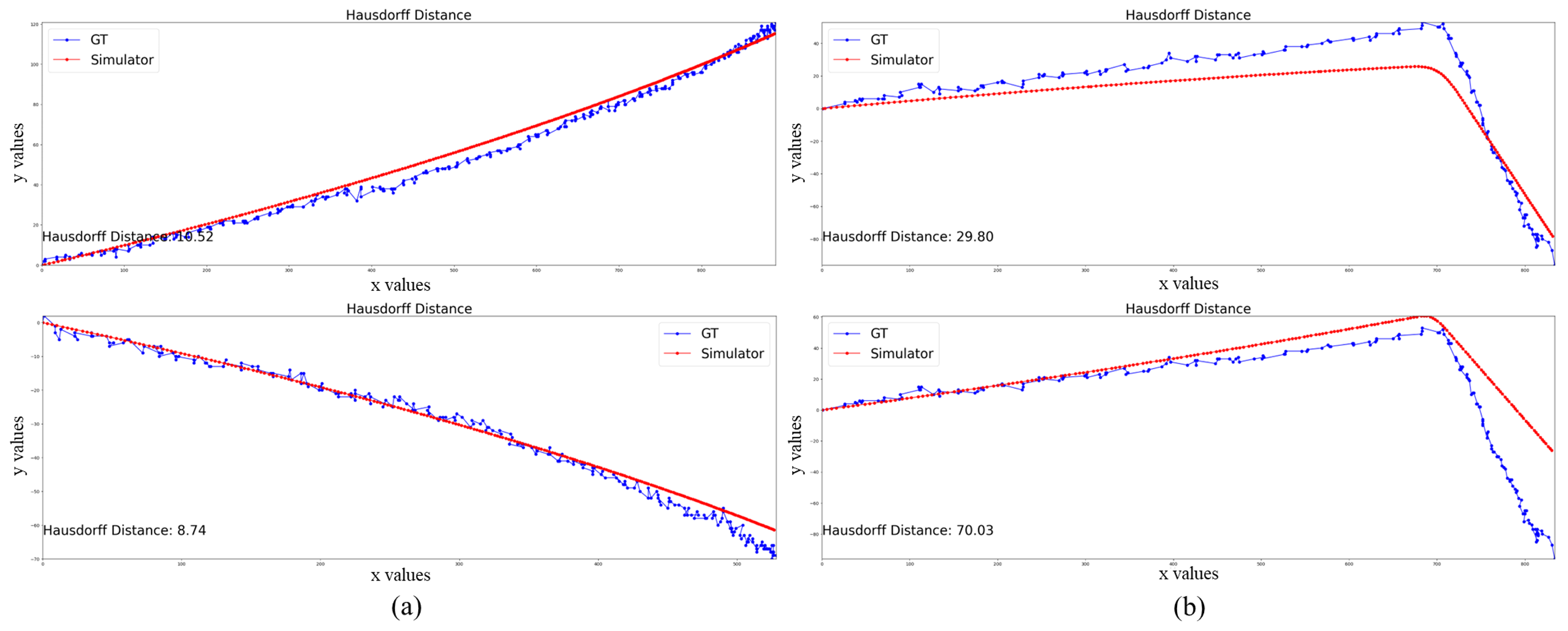
Figure A2 presents representative examples comparing real-world trajectories (GT) with simulated trajectories. In general, trajectory discrepancies are larger in collision cases than in non-collision cases, because impacts alter the stone’s position, velocity, and rotational direction, which can lead to larger deviations.
We quantify the trajectory discrepancy using the Hausdorff distance (cm) between the simulated and video-extracted GT 2D trajectories, computed on trajectory point sets restricted to the ROI. The Hausdorff distance measures the worst-case spatial deviation between two point sets, i.e., the maximum of the closest-point distances, and thus provides a conservative indicator of trajectory mismatch. As reported in Table A2, the final calibrated simulator achieves a mean Hausdorff discrepancy of 2.59 cm over six top-view clips. The discrepancy is larger for collision cases (mean 4.98 cm) than for non-collision cases (mean 1.39 cm), reflecting the additional complexity introduced by impacts. The largest observed discrepancy among the evaluated clips is 6.98 cm.
Figure A2. Representative trajectory overlays used for video-based calibration within the ROI. In all panels, the simulated trajectory is shown in red and the ground-truth (GT) 2D trajectory extracted from the top-view footage is shown in blue. (a) Example shots without collisions; (b) example shots with collisions. The trajectory discrepancy is quantified using the Hausdorff distance (in millimeters) computed between the simulated and GT trajectories restricted to the ROI.
Mathematics 14 00403 g0a2
Table A2. Quantitative trajectory discrepancy for the final calibrated simulator parameters on six top-view clips. The discrepancy is measured by the Hausdorff distance between the simulated and video-extracted 2D trajectories.
ClipCollisionDuration (s)FramesHausdorff Dist (cm)
Video 1No8.332500.87
Video 2No10.43121.96
Video 3Yes6.571972.98
Video 4No8.702611.69
Video 5No10.873291.05
Video 6Yes5.831746.98
Mean (all)2.59
Mean (non-collision)1.39
Mean (collision)4.98

References

  1. Hansen, W. Curling: The History, the Players, the Game; Foreword by Kevin Martin; Key Porter Books: Toronto, ON, Canada, 1999. [Google Scholar]
  2. Hu, C.; Zhao, Y.; Wang, Z.; Du, H.; Liu, J. Games for artificial intelligence research: A review and perspectives. IEEE Trans. Artif. Intell. 2024, 5, 5949–5968. [Google Scholar] [CrossRef] [Scilit]
  3. Mnih, V.; Kavukcuoglu, K.; Silver, D.; Rusu, A.A.; Veness, J.; Bellemare, M.G.; Graves, A.; Riedmiller, M.; Fidjeland, A.K.; Ostrovski, G.; et al. Human-level control through deep reinforcement learning. Nature 2015, 518, 529–533. [Google Scholar] [CrossRef] [Scilit] [PubMed]
  4. Silver, D.; Huang, A.; Maddison, C.J.; Guez, A.; Sifre, L.; Van Den Driessche, G.; Schrittwieser, J.; Antonoglou, I.; Panneershelvam, V.; Lanctot, M.; et al. Mastering the game of Go with deep neural networks and tree search. Nature 2016, 529, 484–489. [Google Scholar] [CrossRef] [Scilit] [PubMed]
  5. Silver, D.; Schrittwieser, J.; Simonyan, K.; Antonoglou, I.; Huang, A.; Guez, A.; Hubert, T.; Baker, L.; Lai, M.; Bolton, A.; et al. Mastering the game of go without human knowledge. Nature 2017, 550, 354–359. [Google Scholar] [CrossRef] [Scilit] [PubMed]
  6. Li, J.; Koyamada, S.; Ye, Q.; Liu, G.; Wang, C.; Yang, R.; Zhao, L.; Qin, T.; Liu, T.Y.; Hon, H.W. Suphx: Mastering mahjong with deep reinforcement learning. arXiv 2020, arXiv:2003.13590. [Google Scholar] [CrossRef] [Scilit]
  7. Zha, D.; Xie, J.; Ma, W.; Zhang, S.; Lian, X.; Hu, X.; Liu, J. Douzero: Mastering doudizhu with self-play deep reinforcement learning. In Proceedings of the International Conference on Machine Learning, PMLR, Virtual, 18–24 July 2021; pp. 12333–12344. [Google Scholar]
  8. Han, Y.; Zhou, Q.; Duan, F. A game strategy model in the digital curling system based on NFSP. Complex Intell. Syst. 2021, 8, 1857–1863. [Google Scholar] [CrossRef] [Scilit]
  9. Lin, J.; Gong, Y.; Zhao, J.; Zhou, W.; Li, H. Mastering curling with rl-revised decision tree. In Proceedings of the 2023 IEEE Conference on Games (CoG), Boston, MA, USA, 21–24 August 2023; IEEE: Piscataway, NJ, USA, 2023; pp. 1–8. [Google Scholar]
  10. Świechowski, M.; Godlewski, K.; Sawicki, B.; Mańdziuk, J. Monte Carlo tree search: A review of recent modifications and applications. Artif. Intell. Rev. 2023, 56, 2497–2562. [Google Scholar] [CrossRef] [Scilit]
  11. Yee, T.; Lisỳ, V.; Bowling, M.H.; Kambhampati, S. Monte Carlo Tree Search in Continuous Action Spaces with Execution Uncertainty. In Proceedings of the IJCAI, New York, NY, USA, 9–15 July 2016; pp. 690–697. [Google Scholar]
  12. Kocsis, L.; Szepesvári, C. Bandit based monte-carlo planning. In Proceedings of the European Conference on Machine Learning, Berlin, Germany, 18–22 September 2006; Springer: Berlin/Heidelberg, Germany, 2006; pp. 282–293. [Google Scholar]
  13. Won, D.O.; Müller, K.R.; Lee, S.W. An adaptive deep reinforcement learning framework enables curling robots with human-like performance in real-world conditions. Sci. Robot. 2020, 5, eabb9764. [Google Scholar] [CrossRef] [Scilit] [PubMed]
  14. Lee, K.; Kim, S.A.; Choi, J.; Lee, S.W. Deep reinforcement learning in continuous action spaces: A case study in the game of simulated curling. In Proceedings of the International Conference on Machine Learning, PMLR, Stockholm, Sweden, 10–15 July 2018; pp. 2937–2946. [Google Scholar]
  15. Heinrich, J.; Silver, D. Deep reinforcement learning from self-play in imperfect-information games. arXiv 2016, arXiv:1603.01121. [Google Scholar]
  16. Oberlin, P. Curling Tactics Analysis with Reinforcement Learning. Master’s Thesis, ETH Zurich, Zürich, Switzerland, 2025. [Google Scholar] [CrossRef]
  17. Silva, C.R.; Bowling, M.; Lelis, L.H. Teaching people by justifying tree search decisions: An empirical study in curling. J. Artif. Intell. Res. 2021, 72, 1083–1102. [Google Scholar] [CrossRef] [Scilit]
  18. Haarnoja, T.; Zhou, A.; Abbeel, P.; Levine, S. Soft actor-critic: Off-policy maximum entropy deep reinforcement learning with a stochastic actor. In Proceedings of the International Conference on Machine Learning, PMLR, Stockholm, Sweden, 10–15 July 2018; pp. 1861–1870. [Google Scholar]
  19. Yamamoto, M.; Kato, S.; Iizuka, H. Digital curling strategy based on game tree search. In Proceedings of the 2015 IEEE Conference on Computational Intelligence and Games (CIG), Tainan, Taiwan, 31 August–1 September 2015; IEEE: Piscataway, NJ, USA, 2015; pp. 474–480. [Google Scholar]
  20. Xiao, Q.; Li, Z.; Wang, X.; Liu, Y.; Li, Y.; Yang, C.; Li, F. Policy decision of curling in real competition scenes. Complex Intell. Syst. 2023, 9, 3301–3312. [Google Scholar] [CrossRef] [Scilit]
  21. World Curling Federation. Le Gruyère AOP European Curling Championships 2023—Men’s Game Records; World Curling Federation: Perth, Scotland, 2023. [Google Scholar]
  22. World Curling Federation. The Rules of Curling and Rules of Competition; World Curling Federation: Perth, Scotland, 2023. [Google Scholar]
Figure 1. Representation of the curling sheet, captured from the custom simulator, including key game boundaries.
Mathematics 14 00403 g001
Figure 2. Average reward per episode in Phase 1 (top) and Phase 2 (bottom). Solid lines show the mean over three independent training runs with random seeds 8, 10, and 13, and the shaded region denotes ± 1 standard deviation.
Mathematics 14 00403 g002
Figure 3. Out-of-sheet ratio as a function of the sensitivity of R area . The out-of-sheet ratio is computed as the number of out-of-sheet stones divided by the total number of thrown stones, aggregated over 30 self-play matches.
Mathematics 14 00403 g003
Figure 4. Examples of the AI agent executing strategic shots. (a-1,a-2) Guard shot, (b-1,b-2) Freeze shot, (c-1,c-2) Come-around shot, and (d-1,d-2) Hit & Roll shot. The trajectories of the agent’s executed shots are highlighted in fluorescent green, while the surrounding stone movements are depicted in fluorescent purple. In contrast, the actual player’s shot trajectories are shown in fluorescent purple, with the surrounding stone movements displayed in fluorescent green. This visualization allows for comparative analysis of AI and human strategies.
Mathematics 14 00403 g004
Table 1. Reproducibility details and key hyperparameters used in all experiments.
SACA2CPPO
General
Episode definition1 end (16 shots)1 end (16 shots)1 end (16 shots)
Discount factor γ 0.970.970.97
Optimization
OptimizerAdamAdamAdam
Learning rate 3 × 10 4 1 × 10 4 1 × 10 4
Batch size25625632
Gradient steps per update11616
Algorithm-specific
Replay buffer size4 k
Target smoothing τ 0.005
Entropy temperature α auto
Target entropy 3
PPO clip ϵ 0.2
Rollout length8 steps128 steps
Compute Resources
GPUNVIDIA RTX A6000 (48 GB)
CPU/RAMIntel(R) Xeon(R) Silver 5215R/128 GB RAM
SoftwareUbuntu 20.04, Python 3.13.5, PyTorch 2.0.1, CUDA 11.8
Table 2. Head-to-head performance of RL agents in the curling simulator. Each entry reports results over 30 matches, where one match consists of 10 ends, and the random seed is resampled for each match. Win–Draw–Loss (Red) denotes match outcomes from the Red agent’s perspective. Score Avg (R–Y) is the per-match total score averaged over 30 matches (mean ± std across matches), where the total score is the sum of end scores within a match. End Score Avg (R–Y) is the corresponding per-end average, i.e., Score Avg divided by 10. For reference, under standard curling scoring (maximum 8 points per end), the theoretical upper bound of a match total is 8 × 10 points.
CompetitionResult
Agent (Red)Agent (Yellow)MatchesWin–Draw–Loss (Red)Score Avg (R–Y)End Score Avg (R–Y)
Phase 2 vs. Phase 2
SAC (Phase 2)A2C (Phase 2)3024–0–6 11.43 ( ± 4.07 ) 4.93 ( ± 2.72 ) 1.14 ( ± 0.41 ) 0.49 ( ± 0.27 )
SAC (Phase 2)PPO (Phase 2)3030–0–0 16.37 ( ± 3.83 ) 4.80 ( ± 2.50 ) 1.64 ( ± 0.38 ) 0.48 ( ± 0.25 )
A2C (Phase 2)PPO (Phase 2)3011–0–19 6.93 ( ± 3.38 ) 7.63 ( ± 3.11 ) 0.69 ( ± 0.34 ) 0.76 ( ± 0.31 )
Phase 2 vs. Phase 1
SAC (Phase 2)SAC (Phase 1)3023–0–7 11.53 ( ± 4.93 ) 6.07 ( ± 2.77 ) 1.15 ( ± 0.49 ) 0.61 ( ± 0.28 )
SAC (Phase 2)A2C (Phase 1)3027–0–3 13.80 ( ± 3.57 ) 4.07 ( ± 2.37 ) 1.38 ( ± 0.36 ) 0.41 ( ± 0.24 )
SAC (Phase 2)PPO (Phase 1)3027–0–3 12.90 ( ± 3.57 ) 5.4 ( ± 2.61 ) 1.29 ( ± 0.36 ) 0.54 ( ± 0.26 )
Table 3. Performance evaluation of ablation models in the curling simulator. Results are reported over 30 matches, each consisting of 10 ends, and the random seed is resampled for each match. “No s t game , R score ” removes all game-context state terms and score-based reward components. “No ψ ” removes curl effects by fixing angular velocity to zero ( ψ = 0 ). Win–Draw–Loss (Red) denotes match outcomes from the Red agent’s perspective. Score Avg (R–Y) is the per-match total score averaged over 30 matches (mean ± std across matches), and End Score Avg (R–Y) is Score Avg divided by 10.
CompetitionResult
Agent (Red)Agent (Yellow)MatchesWin–Draw–Loss (Red)Score Avg (R–Y)End Score Avg (R–Y)
Proposed vs. Variants
Proposed (SAC-Phase 2)No s t game , R score 3030–0–0 16.50 ( ± 4.26 ) 1.03 ( ± 0.09 ) 1.65 ( ± 0.43 ) 0.10 ( ± 0.01 )
Proposed (SAC-Phase 2)No ψ 3027–0–3 11.77 ( ± 3.31 ) 5.33 ( ± 2.23 ) 1.18 ( ± 0.33 ) 0.53 ( ± 0.22 )
Proposed (SAC-Phase 2)No s t game , R score , ψ 3030–0–0 20.47 ( ± 4.17 ) 0.9 ( ± 0.92 ) 2.05 ( ± 0.42 ) 0.09 ( ± 0.02 )
Variants vs. Variants
No s t game , R score No ψ 300–0–30 1.40 ( ± 1.18 ) 8.13 ( ± 2.29 ) 0.14 ( ± 0.12 ) 0.81 ( ± 0.23 )
No s t game , R score No s t game , R score , ψ 3023–0–7 3.23 ( ± 1.23 ) 1.25 ( ± 1.27 ) 0.32 ( ± 0.12 ) 0.13 ( ± 0.13 )
No ψ No s t game , R score , ψ 3030–0–0 16.00 ( ± 1.97 ) 0.40 ( ± 0.76 ) 1.60 ( ± 0.20 ) 0.04 ( ± 0.08 )
Disclaimer/Publisher’s Note: The statements, opinions and data contained in all publications are solely those of the individual author(s) and contributor(s) and not of MDPI and/or the editor(s). MDPI and/or the editor(s) disclaim responsibility for any injury to people or property resulting from any ideas, methods, instructions or products referred to in the content.