An η-Power Stochastic Log-Logistic Diffusion Process: Statistical Computation and Application to Individuals Using the Internet in the United States

Abstract

A new family of stochastic $\eta$-power log-logistic diffusion processes was introduced and defined based on the classical log-logistic diffusion model. The probabilistic characteristics of the proposed process were derived through an analysis of the associated stochastic differential equation (SDE), including its explicit expressions, the transition probability density function, and the conditional and non-conditional mean functions. The statistical inference of the model was studied, and parameter estimation was performed using the maximum likelihood method based on discrete sampling paths. The proposed probabilistic and statistical framework was applied to data on individuals using the Internet in the United States to assess the practical performance of the model. The empirical results demonstrated that the inclusion of a power in the process improved the goodness of fit compared with the classical formulation, providing better agreement with the observed data. Finally, a small Monte Carlo experiment was performed to examine the robustness of the estimation procedure.

1. Introduction

Diffusion models are commonly employed to describe stochastic phenomena evolving over time in the presence of random fluctuations and are used to model many realistic stochastic systems in which uncertainty exists. Such models arise in a wide range of applications across multiple fields, including finance, engineering, biology, and economics. In many practical situations, deterministic formulations may be inadequate to fully capture this variability. Stochastic diffusion processes provide an appropriate alternative and are typically defined as solutions of stochastic differential equations of the form

$$dx\left(t\right)=f(t,x(t),\theta )dt+\sigma (t,x(t),\theta )dW\left(t\right).$$

(1)

where $f(t,x(t),\theta )$ and $\sigma (t,x(t),\theta )$ are known functions representing the drift and diffusion coefficients, respectively, $\theta$ is a vector of unknown parameters, and $W\left(t\right)$ is a standard Wiener process. For further details, see [1,2,3,4,5,6]. This paper concerns a family of diffusion processes defined by an $\eta$-power log-logistic diffusion model. The paper is devoted to the analytical properties of the model, the statistical computation of its parameters, and its application to modeling individuals using the Internet in the United States.

Considerable research effort has been devoted to the development of stochastic diffusion models for describing time-dependent phenomena subject to random fluctuations. In particular, diffusion processes derived from parametric distributions have been widely investigated due to their analytical tractability and relevance in statistical modeling. Within this framework, several diffusion models have been proposed and studied in the literature, including the Log-Logistic [7], Schumer [8], Lomax [9], Weibull [10], Square–Brennan–Schwartz [11], Brennan–Schwartz [12], Gamma [13], Gompertz [14], Rayleigh [15], Lundqvist–Korf [16], Generalized Gamma-like curve [17], and Sine-like [18] diffusion processes. In recent years, power-type transformations have been incorporated into diffusion models to enhance modeling flexibility and improve empirical performance. For example, Chakroune et al. [19] introduce a new family of Rayleigh processes defined by the power of the stochastic Rayleigh diffusion model. In this stage, we also refer to the work of Gutiérrez et al. [20], who modeled the natural gas consumption in Spain through a new stochastic gamma diffusion process driven by a power of $\tau$. A $\gamma$-power stochastic Lundqvist–Korf diffusion process ($\gamma$-SLKDP) has been developed and analyzed from computational and simulation perspectives [21]. These studies demonstrate the effectiveness of power-based diffusion formulations for capturing diverse dynamic behaviors while maintaining computational feasibility. Nevertheless, further development of power-driven diffusion models with explicit probabilistic characteristics and reliable inference procedures remains of practical interest.

Motivated by these developments, a new family of stochastic $\eta$-power log-logistic diffusion processes was introduced and defined based on the classical log-logistic diffusion model [7]. Our main contributions in this paper can be summarized as follows. First, a new family of diffusion processes is introduced for modeling time series data exhibiting different trend behaviors through the inclusion of a power parameter in the model formulation. Second, the fundamental theoretical and probabilistic properties of the proposed process are investigated, including the existence and uniqueness of the solution, the derivation of the transition probability density function, the computation of the moments, and the analysis of both the trend and conditional trend functions. Third, the parameters of the proposed diffusion process are estimated using the maximum likelihood method. Fourth, the applicability of the proposed diffusion model is illustrated using a real-world data set, and its performance is compared with an existing power-transformed diffusion model. Finally, simulation experiments based on parameter estimates obtained from the real data are performed to assess the consistency of the maximum likelihood estimators. The remainder of this paper is organized as follows. Section 2 introduces background material and preliminary concepts. Section 3 summarizes the main results and highlights the principal contributions of the paper. Section 4 describes the methodology adopted in this study, and defines the proposed stochastic diffusion process and its characteristics, including the solution of the process, the transition probability density function (TPDF), and the moments. Section 5 is dedicated to estimating the model’s parameters using the maximum likelihood (ML) estimation method, based on discrete sampling of the process. In Section 6, the performance of the proposed process is evaluated using a real-world data set. The accuracy of the forecast is assessed using a global descriptive measure of the goodness of fit (GOF) between the adjusted values and the real data using the sampling variance. The $\gamma$-power stochastic Lundqvist–Korf diffusion process is also used as a comparison model. Furthermore, a small Monte Carlo experiment is conducted to assess the robustness of the estimation procedure. Section 7 presents a discussion of the tables and figures presented in this paper. Finally, Section 8 offers concluding remarks.

2. Background

This section provides background material to support the understanding of the proposed stochastic model.

2.1. Preliminaries

This subsection begins with a brief review of the definition of Brownian motion, a fundamental example of a stochastic process. The following definition is adopted from [1].

Definition 1.

A Brownian motion (or a standard one-dimensional Wiener process) is a continuous, adapted process ${\left(W_t\right)}_{t\ge 0}$, defined on some probability space $(\Omega ,\mathcal{F},P)$, with the properties $W_0=0$ a.s., and for $0\le s<t$, the increment $W_t-W_s$ is independent of ${\mathcal{F}}_s$ and is normally distributed with mean zero and variance $t-s$.

A stochastic differential equation is an equation of the form

$$dX\left(t\right)=f(t,X(t),\theta )dt+\sigma (t,X(t),\theta )dW\left(t\right),t\in [0,T];T>0,$$

(2)

where $X\left(t\right)$ denotes the state process and $f(t,x(t),\theta )$ denotes the drift coefficient, which characterizes the deterministic trend and long-term behavior of the process, while $\sigma (t,x(t),\theta )$ is the diffusion coefficient governing the intensity of random fluctuations. The process $W\left(t\right)$ denotes a standard Brownian motion (Wiener process), representing the source of stochastic perturbations. The parameter vector $\theta \in \mathrm{\Theta }\subset {\mathbb{R}}^p$ contains the unknown model parameters to be estimated from observed data and belongs to an admissible parameter space ensuring the well-posedness of the model. Morally, Equation (2) models the balance between deterministic dynamics and random variability and provides a flexible framework for describing real-world time series evolving under uncertainty. Under suitable regularity conditions, the SDE (2) admits a well-defined stochastic process solution $X\left(t\right)$, which is commonly referred to as a diffusion process.

The classical Itô formula is recalled below, which plays a fundamental role in the analysis of stochastic differential equations; see [1] for further details.

Definition 2 (Itô Formula).

Let $X\left(t\right)$ be a stochastic process satisfying the stochastic differential equation

$$dX\left(t\right)=\mu (t,X(t\left)\right)dt+\sigma (t,X(t\left)\right)dW\left(t\right),$$

where $W\left(t\right)$ is a standard Brownian motion. Let $f(t,x)\in C^{1,2}([0,T]\times \mathbb{R})$, that is, f is once continuously differentiable in t and twice continuously differentiable in x. Then, the process $Y\left(t\right)=f(t,X(t\left)\right)$ satisfies

$$\begin{array}{cc}\hfill df(t,X(t\left)\right)& =\left({\displaystyle \frac{\partial f}{\partial t}}(t,X\left(t\right))+\mu (t,X\left(t\right)){\displaystyle \frac{\partial f}{\partial x}}(t,X\left(t\right))+{\displaystyle \frac{1}{2}}{\sigma }^2(t,X\left(t\right)){\displaystyle \frac{{\partial }^{2}f}{\partial x^2}}(t,X\left(t\right))\right)dt\hfill \\ \hfill & +\sigma (t,X\left(t\right)){\displaystyle \frac{\partial f}{\partial x}}(t,X\left(t\right))dW\left(t\right).\hfill \end{array}$$

2.2. An Overview of the Stochastic Log-Logistic Model

Throughout this subsection, we follow the formulation and results established in [7], to which the reader is referred for further details. Let $\{X\left(t\right),t\in [t_1,T],t_1>0\}$ be a diffusion process with values in $(0,\infty )$, where $X\left(t\right)$ is a stochastic log-logistic diffusion process, then $X\left(t\right)$ satisfies the following It$\widehat{\mathrm{o}}$’s SDE

$$dX\left(t\right)=\left[{\displaystyle \frac{-\ln \left(b\right)\phi \left(t\right)}{t(a+\phi (t\left)\right)}}\right]X\left(t\right)dt+\sigma X\left(t\right)dW\left(t\right);X\left(t_1\right)=x_1,$$

(3)

with $\phi \left(t\right)=b^{\ln \left(t\right)}$. And, $0<\sigma$, $0<a<1$, and $0<b<1$ are the parameters. The SED (3) has a unique solution is given by

$$X\left(t\right)=x_1\left({\displaystyle \frac{a+\phi \left(t_1\right)}{a+\phi \left(t\right)}}\right)\exp \left(-{\displaystyle \frac{{\sigma }^2}{2}}(t-t_1)+\sigma \left(W\left(t\right)-W\left(t_1\right)\right)\right).$$

(4)

From this, the process ($X\left(t\right)|X\left(s\right)=x_s$) where $s<t$ is distributed as log-normal distribution ${\mathrm{\Lambda }}_1(\mu (s,t,x_s),{\sigma }^2(t-s))$, where $\mu (s,t,x_s)$ is given by

$$\begin{array}{c}\hfill \mu (s,t,x)=\log \left(x_s\right)+\log \left({\displaystyle \frac{a+\phi \left(s\right)}{a+\phi \left(t\right)}}\right)-{\displaystyle \frac{{\sigma }^2}{2}}(t-s).\end{array}$$

Therefore, the TPDF of the process has the following form

$$\begin{array}{c}\hfill f(y,t|x_s,s)={\displaystyle \frac{1}{y}}{\left[2\pi {\sigma }^2(t-s)\right]}^{-1/2}\exp \left(-{\displaystyle \frac{{[\log \left(y\right)-\mu (s,t,x_s)]}^2}{2{\sigma }^2(t-s)}}\right).\end{array}$$

(5)

3. Main Results

The main objective of this study is to address the following research question:

How can a flexible stochastic diffusion model be constructed and statistically inferred in order to accurately describe, simulate, and forecast real-world time series?

To answer this question, we introduce a new stochastic model, referred to as the $\eta$-power stochastic log-logistic diffusion process, which is obtained by applying a power transformation to the classical log-logistic diffusion process. This construction extends classical diffusion models by incorporating a flexible drift structure and an analytically tractable transition density. The proposed process is designed to capture the main dynamic features observed in practical applications while preserving mathematical tractability for statistical inference and numerical implementation. The main results of this paper can be summarized as follows:

• We propose the $\eta$-power stochastic log-logistic diffusion process obtained via a power transformation of the classical log-logistic diffusion process as a new class of diffusion models;
• We derive explicit analytical expressions for the transition probability density function of the proposed process, which enables efficient likelihood-based parameter estimation;
• Maximum likelihood estimation procedures for the model parameters are developed based on discrete observations, together with the corresponding estimated trend functions and confidence bands;
• The performance of the model is validated through an application to real-world data, demonstrating improved fitting and forecasting capability compared with the classical log-logistic diffusion model, and it is further compared with the $\gamma$-power Stochastic Lundqvist–Korf Diffusion model, showing superior fitting performance;
• A simulation scheme is presented to generate sample paths of the proposed diffusion process, illustrating its numerical stability and practical implementation.

4. The Proposed Model

This section presents the methodological framework adopted in this study and introduces our new one-dimensional stochastic diffusion process.

4.1. Methodology

This subsection describes the construction of the proposed stochastic model and outlines the methodological framework adopted in this study. Let ${\left(X_t\right)}_{t\ge 0}$ denote the classical log-logistic diffusion process. We construct a new process ${\left(Y_t\right)}_{t\ge 0}$ by applying a power transformation of the form

$$Y_t=X_t^{\eta },\eta >0.$$

(6)

Using Itô’s formula, the stochastic differential equation satisfied by $\left(Y_t\right)$ is derived explicitly, leading to the definition of the $\eta$-power stochastic log-logistic diffusion process. The explicit drift and diffusion coefficients of the transformed process are then obtained and used to derive its transition probability density function, which forms the basis for statistical inference and numerical implementation.

4.2. The $\eta$-Power Stochastic Log-Logistic Diffusion Process ($\eta$-SLLDP)

Let $\{X\left(t\right),t\in [t_1,T],t_1>0\}$ be a stochastic log-logistic diffusion process. Then, the $\eta$-SLLDP is defined by

$$X_{\eta }\left(t\right)=X^{\eta }\left(t\right);\eta \in {\mathbb{R}}^{*},$$

(7)

where ${\mathbb{R}}^{*}$ denotes the set of all non-zero real numbers. The process $\{X_{\eta }\left(t\right),t\in [t_1,T],t_1>0\}$ is the non-homogeneous diffusion process with values in $(0,\infty )$. By applying It$\widehat{\mathrm{o}}$’s formula to (7) we have the following SDE

$$d{X}_{\eta }\left(t\right)=\left[{\displaystyle \frac{-\eta \ln \left(b\right)\phi \left(t\right)}{t(a+\phi (t\left)\right)}}+{\displaystyle \frac{\eta (\eta -1){\sigma }^2}{2}}\right]X_{\eta }\left(t\right)dt+\eta \sigma X_{\eta }\left(t\right)dW\left(t\right),$$

(8)

where $\phi \left(t\right)=b^{\ln \left(t\right)}$. And $0<\sigma$, $0<a<1$, and $0<b<1$ are the parameters. In the following, we show the existence and uniqueness of the solution for the SDE given in (8). To achieve this goal, it is sufficient to verify uniform Lipschitz and linear growth conditions, see [22], which are realized in the following theorem.

Theorem 1.

The SDE in (8) admits a unique solution.

Proof. 

Let $f(t,x(t\left)\right)$ denotes the drift coefficient, and $B^{1/2}(t,x\left(t\right))$ denotes the diffusion coefficient for the SDE given in (8). On the one hand, consider $x,y\in [0,\infty )$ and $t\in [t_1,T]$. It then follows that

$$\begin{array}{cc}\hfill & |f(t,x)-f(t,y)|+|\sqrt{B(t,x)}-\sqrt{B(t,y)}|\hfill \\ \hfill & =|f(t,x-y)|+|\sqrt{B(t,x-y)}|,\hfill \\ \hfill & =\left|\left({\displaystyle \frac{-\eta \ln \left(b\right)\phi \left(t\right)}{t(a+\phi (t\left)\right)}}+{\displaystyle \frac{\eta (\eta -1){\sigma }^2}{2}}\right)(x-y)\right|+|\eta \sigma (x-y)|,\hfill \\ \hfill & =\left(\left|\left({\displaystyle \frac{-\eta \ln \left(b\right)\phi \left(t\right)}{t(a+\phi (t\left)\right)}}+{\displaystyle \frac{\eta (\eta -1){\sigma }^2}{2}}\right)\right|+|\eta \sigma |\right)|x-y|,\hfill \\ \hfill & \le \left(\underset{t_1\le t\le T}{\sup }\left|\left({\displaystyle \frac{-\eta \ln \left(b\right)\phi \left(t\right)}{t(a+\phi (t\left)\right)}}+{\displaystyle \frac{\eta (\eta -1){\sigma }^2}{2}}\right)\right|+|\eta \sigma |\right)\left|x-y\right|.\hfill \end{array}$$

Therefore, the process satisfies a uniform Lipschitz. On the other hand, this process satisfies the linear growth condition, as for $y=0$, we have

$$\begin{array}{cc}\hfill & {|f(t,x)|}^2+{|\sqrt{B(t,x)}|}^2\le {\left(|f(t,x)|+|\sqrt{B(t,x)}|\right)}^2,\hfill \\ \hfill & \le {\left[\left(\underset{t_1\le t\le T}{\sup }\left|\left({\displaystyle \frac{-\eta \ln \left(b\right)\phi \left(t\right)}{t(a+\phi (t\left)\right)}}+{\displaystyle \frac{\eta (\eta -1){\sigma }^2}{2}}\right)\right|+|\eta \sigma |\right)|x|\right]}^2,\hfill \\ \hfill & \le {\left(\underset{t_1\le t\le T}{\sup }\left|\left({\displaystyle \frac{-\eta \ln \left(b\right)\phi \left(t\right)}{t(a+\phi (t\left)\right)}}+{\displaystyle \frac{\eta (\eta -1){\sigma }^2}{2}}\right)\right|+|\eta \sigma |\right)}^2{(1+|x|)}^2.\hfill \end{array}$$

Thus, there is an almost surely (a.s.) continuous process $\{x\left(t\right),t\in [t_1,T];t_1>0\}$ that is a.s. the unique solution of the SDE (8). □

The solution of (8) can be obtained using the formula $X_{\eta }\left(t\right)=X^{\eta }\left(t\right)$ and the Equation (4), from which we have

$$X_{\eta }\left(t\right)=X_{\eta }\left(t_1\right){\left({\displaystyle \frac{a+\phi \left(t_1\right)}{a+\phi \left(t\right)}}\right)}^{\eta }\exp \left(-{\displaystyle \frac{\eta {\sigma }^2}{2}}(t-t_1)+\eta \sigma \left(W\left(t\right)-W\left(t_1\right)\right)\right).$$

(9)

Therefore, the process ($X_{\eta }\left(t\right)|X_{\eta }\left(s\right)=x_s$) is distributed as log-normal distribution ${\mathrm{\Lambda }}_1(m(s,t,x_s),{\eta }^2{\sigma }^2(t-s))$, i.e., $\ln \left(X\right)\sim \mathcal{N}(m(s,t,x_s),{\eta }^2{\sigma }^2(t-s))$, with 

$$\begin{array}{c}\hfill m(s,t,x)=\log \left(x_s\right)+\eta \log \left({\displaystyle \frac{a+\phi \left(s\right)}{a+\phi \left(t\right)}}\right)-{\displaystyle \frac{\eta {\sigma }^2}{2}}(t-s).\end{array}$$

(10)

4.3. The Probability Distribution and Moments of the Process

The TPDF of the $\eta$-SLLDP has the following form:

$$\begin{array}{c}\hfill f(y,t|x_s,s)={\displaystyle \frac{1}{y}}{\left[2\pi {\eta }^2{\sigma }^2(t-s)\right]}^{-1/2}\exp \left(-{\displaystyle \frac{{[\log \left(y\right)-m(s,t,x_s)]}^2}{2{\eta }^2{\sigma }^2(t-s)}}\right).\end{array}$$

(11)

Taking into account that $X_{\eta }\left(t\right)|X_{\eta }\left(s\right)=x_s$ is distributed according to ${\mathrm{\Lambda }}_1(m(s,t,x_{ts}),$${\eta }^2{\sigma }^2(t-s)),$ and taking into account the properties of this distribution, the $n^{th}$ conditional moment of $X_{\eta }\left(t\right)$ given $X_{\eta }\left(s\right)$ is

$$\begin{array}{cc}\hfill E[X_{\eta }^n\left(t\right)|X_{\eta }\left(s\right)=x_s]& =\exp \left(nm(s,t,x_s)+{\displaystyle \frac{n^2{\eta }^2{\sigma }^2}{2}}(t-s)\right),\hfill \\ \hfill & =\exp \left(\log \left(x_s^n\right)+n\eta \log \left({\displaystyle \frac{a+\phi \left(s\right)}{a+\phi \left(t\right)}}\right)-{\displaystyle \frac{n\eta {\sigma }^2}{2}}(t-s)+{\displaystyle \frac{n^2{\eta }^2{\sigma }^2}{2}}(t-s)\right),\hfill \\ \hfill & =x_s^n{\left({\displaystyle \frac{a+\phi \left(s\right)}{a+\phi \left(t\right)}}\right)}^{n\eta }\exp \left({\displaystyle \frac{n(n\eta -1){\sigma }^2\eta }{2}}(t-s)\right).\hfill \end{array}$$

Then, the conditional mean, which is considered as the trend function $(n=1)$ of the process, is

$$\begin{array}{c}\hfill E[X_{\eta }\left(t\right)|X_{\eta }\left(s\right)=x_s]=x_s{\left({\displaystyle \frac{a+\phi \left(s\right)}{a+\phi \left(t\right)}}\right)}^{\eta }\exp \left({\displaystyle \frac{(\eta -1){\sigma }^2\eta }{2}}(t-s)\right).\end{array}$$

(12)

On the other hand, the mean function (MF) or the unconditional trend of the process under the assumption that $P(x\left(t_1\right)=x_1)=1$ is given by

$$\begin{array}{cc}\hfill E\left[X_{\eta }\left(t\right)\right]& =x_1{\left({\displaystyle \frac{a+\phi \left(t_1\right)}{a+\phi \left(t\right)}}\right)}^{\eta }\exp \left({\displaystyle \frac{(\eta -1){\sigma }^2\eta }{2}}(t-t_1)\right).\hfill \end{array}$$

(13)

5. Statistical Inference and Parameter Estimation of the Process

In this section, we study the ML estimation of the model parameters, which, based on Zenha’s theorem [23], leads to the corresponding aforementioned estimated and conditional estimated mean functions.

5.1. ML Estimates

Given the explicit expression of the TPDF of the process, we can estimate the parameters that appear in the drift and diffusion functions using ML method. The following proposition provides the log-likelihood function associated with the discretely observed $\eta$-SLLDP.

Proposition 1.

Let ${\left\{X_{\eta }\left(t\right)\right\}}_{t\ge 0}$ be a η-SLLDP observed at discrete times $0<t_1<t_2<\cdots <t_n=T$, and denote $x_j=X_{\eta }\left(t_j\right)$. Assume an equidistant sampling scheme $t_{j+1}-t_j=h$ for $j=1,\dots ,n-1$, and let the parameter $\mathit{\theta }={(a,b,{\sigma }^2)}^T$. Taking the initial condition as fixed, i.e., $P(X_{\eta }\left(t_1\right)=x_1)=1$, the log-likelihood function $\mathsf{\ell }(a,b,{\sigma }^2)$ is

$$\begin{array}{cc}\mathsf{\ell }(a,b,{\sigma }^2)=& -{\displaystyle \frac{n-1}{2}}\log \left(2\pi {\eta }^{2}h\right)-{\displaystyle \frac{n-1}{2}}\log \left({\sigma }^2\right)-\underset{j=1}{\sum ^{n-1}}\log \left(x_{j+1}\right)\\ & -{\displaystyle \frac{1}{2{\eta }^2{\sigma }^{2}h}}\underset{j=1}{\sum ^{n-1}}{\left[\log \left({\displaystyle \frac{x_{j+1}}{x_j}}\right)-\eta \log \left({\displaystyle \frac{a+\phi \left(t_j\right)}{a+\phi \left(t_{j+1}\right)}}\right)+{\displaystyle \frac{\eta {\sigma }^2}{2}}h\right]}^2.\end{array}$$

(14)

Proof. 

The likelihood function $\mathcal{L}\left(\mathit{\theta }\right)$ of the parameter $\mathit{\theta }={(a,b,{\sigma }^2)}^T$ can be obtained from Equation (11) as

$$\begin{array}{cc}\hfill & \mathcal{L}\left(\mathit{\theta }\right)=\underset{j=1}{\prod ^{n-1}}f(x_{j+1},t_{j+1}|x_j,t_j),\hfill \\ \hfill & =\underset{j=1}{\prod ^{n-1}}{\displaystyle \frac{1}{x_{j+1}}}{\left[2\pi {\eta }^2{\sigma }^2(t_{j+1}-t_j)\right]}^{-1/2}\exp \left(-{\displaystyle \frac{{\left[\log \left(x_{j+1}\right)-m(j,j+1,x_j)\right]}^2}{2{\eta }^2{\sigma }^2(t_{j+1}-t_j)}}\right),\hfill \\ \hfill & =\underset{j=1}{\prod ^{n-1}}{\displaystyle \frac{1}{x_{j+1}}}{\left[2\pi {\eta }^2{\sigma }^{2}h\right]}^{-1/2}\exp \left(-{\displaystyle \frac{{\left[\log \left(\frac{x_{j+1}}{x_j}\right)-\eta \log \left(\frac{a+\phi \left(t_j\right)}{a+\phi \left(t_{j+1}\right)}\right)+\frac{\eta {\sigma }^2}{2}(t_{j+1}-t_j)\right]}^2}{2{\eta }^2{\sigma }^{2}h}}\right).\hfill \end{array}$$

(15)

Taking logarithms for both sides of (15), we obtain the log-likelihood equation as in (14), and this completes the proof. □

The $\mathsf{\ell }(a,b,{\sigma }^2)$ can be maximized by solving the nonlinear likelihood equation obtained by differentiating $\mathsf{\ell }(a,b,{\sigma }^2)$ with respect to $\mathit{\theta }={(a,b,{\sigma }^2)}^T$. Unfortunately, the estimation of a, b, and ${\sigma }^2$ presents significant difficulties. The associated system of equations becomes extremely complex and admits no explicit analytical solution; therefore, numerical procedures are necessary to obtain these estimates.

5.2. Estimated Mean Functions and Confidence Bounds

The estimated conditional mean function (ECMF) represents the conditional expectation of the process at a future time, given its current observed value and the estimated model parameters. It reflects the short-term predictive behavior of the system and describes how the process is expected to evolve dynamically from a given initial state. In contrast, the estimated mean function (EMF) corresponds to the unconditional expectation of the process and characterizes the overall average trend of the stochastic dynamics over time. While the ECMF captures local and data-driven evolution conditioned on available information, the EMF provides a global description of the long-term behavior of the model. Together, ECMF and EMF offer complementary insight into both predictive performance and structural characteristics of the proposed stochastic process. The conditional mean and the mean of the $\eta$-SLLDP are estimated by replacing the parameters in Equations (12) and (13) with their ML estimators, in view of the invariance property of the ML estimates; see, for example, Theorem [5.28, 308] in [24]. Let $\widehat{a}$, $\widehat{b}$ and ${\widehat{\sigma }}^2$ be the ML estimates of a, b and ${\sigma }^2$, respectively, and let $\widehat{\phi }\left(t\right)={\widehat{b}}^{\ln \left(t\right)}$. Then, the ECMF of the process is

$$\begin{array}{c}\hfill \widehat{E}[X_{\eta }\left(t\right)|X_{\eta }\left(s\right)=x_s]=x_s{\left({\displaystyle \frac{\widehat{a}+\widehat{\phi }\left(s\right)}{\widehat{a}+\widehat{\phi }\left(t\right)}}\right)}^{\eta }\exp \left({\displaystyle \frac{(\eta -1){\widehat{\sigma }}^2\eta }{2}}(t-s)\right).\end{array}$$

(16)

Also, the EMF of the process is

$$\begin{array}{c}\hfill \widehat{E}[X_{\eta }\left(t\right)|X_{\eta }\left(t_1\right)]=x_1{\left({\displaystyle \frac{\widehat{a}+\widehat{\phi }\left(t_1\right)}{\widehat{a}+\widehat{\phi }\left(t\right)}}\right)}^{\eta }\exp \left({\displaystyle \frac{(\eta -1){\widehat{\sigma }}^2\eta }{2}}(t-t_1)\right),\end{array}$$

(17)

taking into account the assumption $P(X_{\eta }\left(t_1\right)=x_1)=1.$ Moreover, the confidence band for the MF of the process is obtained following the procedure described in [25]. The following proposition provides the derivation of the confidence band.

Proposition 2.

Let ${\left\{X\left(t\right)\right\}}_{t\ge 0}$ be an η-SLLDP and assume that $X\left(t_1\right)=x_1$ is fixed. For any $t>t_1$ and $\alpha \in (0,1)$, a $(1-\alpha )100\%$ confidence band (CB) for $X\left(t\right)$ is

$$x_{lower}\left(t\right)\le x\left(t\right)\le x_{upper}\left(t\right)$$

(18)

where

$$\begin{array}{cc}\hfill & x_{lower}\left(t\right)=x_1\exp \left[-Z_{\alpha /2}\eta \sigma \sqrt{t-t_1}+\eta \log \left({\displaystyle \frac{a+\phi \left(t_1\right)}{a+\phi \left(t\right)}}\right)-{\displaystyle \frac{\eta {\sigma }^2}{2}}(t-t_1)\right],\hfill \\ \hfill & x_{upper}\left(t\right)=x_1\exp \left[Z_{\alpha /2}\eta \sigma \sqrt{t-t_1}+\eta \log \left({\displaystyle \frac{a+\phi \left(t_1\right)}{a+\phi \left(t\right)}}\right)-{\displaystyle \frac{\eta {\sigma }^2}{2}}(t-t_1)\right].\hfill \end{array}$$

(19)

And $Z_{\alpha /2}$ is the $(1-\alpha /2)$-quantile of the standard normal distribution.

Proof. 

From Equation (11), we have that for $t>s$, $X\left(t\right)|X(s)$ follows ${\mathrm{\Lambda }}_1(m(s,t,x_s),{\eta }^2{\sigma }^2(t-s))$. Therefore, we have that

$$Z={\displaystyle \frac{\ln \left(X\left(t\right)\right)-m(s,t,x_s)}{\eta \sigma \sqrt{t-s}}}\sim \mathcal{N}(0,1).$$

(20)

Consequently, a $(1-\alpha )100\%$ confidence band for Z is determined by

$$P(-Z_{\alpha /2}\le Z\le Z_{\alpha /2})=1-\alpha ,\mathrm{for}\alpha \in (0,1),$$

(21)

which is equivalent to

$$P\left(m(s,t,x_s)-Z_{\alpha /2}\eta \sigma \sqrt{t-s}\le \ln X\left(t\right)\le m(s,t,x_s)+Z_{\alpha /2}\eta \sigma \sqrt{t-s}\right)=1-\alpha .$$

Exponentiating yields

$$P\left(e^{m(s,t,x_s)-Z_{\alpha /2}\eta \sigma \sqrt{t-s}}\le X\left(t\right)\le e^{m(s,t,x_s)+Z_{\alpha /2}\eta \sigma \sqrt{t-s}}\right)=1-\alpha .$$

Finally, substituting the explicit form of $m(s,t,x_s))$ from Equation (10),

$$\begin{array}{c}\hfill m(s,t,x)=\log \left(x_s\right)+\eta \log \left({\displaystyle \frac{a+\phi \left(s\right)}{a+\phi \left(t\right)}}\right)-{\displaystyle \frac{\eta {\sigma }^2}{2}}(t-s),\end{array}$$

and taking $s=t_1$ and $x_s=x_1$, gives exactly the bounds $x_{\mathrm{lower}}\left(t\right)$ and $x_{\mathrm{upper}}\left(t\right)$ in (19), completing the proof. □

6. Application and Numerical Results

This section presents the real data application and numerical simulations. The $\eta$-SLLDP model is fitted and compared with the $\gamma$-SLKDP [21] model, and numerical computations are performed based on the estimated parameters. All computations in this paper were performed using R software (version 4.3.1) [26].

6.1. Application

This section presents an application of our model to a real-world data set: individuals using the Internet (% of population) in the United States from 1995 to 2023. The data used in this analysis are shown in Table 1; these data are annualized and available in the World Bank database https://databank.worldbank.org/source/world-development-indicators (accessed on 3 December 2025).

Table 1. Individuals using the Internet (% of population) in the United States.

Year	1995	1996	1997	1998	1999	2000
Data	9.2400	16.4000	21.6000	30.1000	35.8000	43.0792
Year	2001	2002	2003	2004	2005	2006
Data	49.0808	58.7854	61.6971	64.7583	67.9681	68.9312
Year	2007	2008	2009	2010	2011	2012
Data	75.0000	74.0000	71.0000	71.6900	69.7295	74.7000
Year	2013	2014	2015	2016	2017	2018
Data	71.4000	73.0000	74.5542	85.5444	87.2749	88.4989
Year	2019	2020	2021	2022	2023
Data	89.4303	90.3447	91.2684	92.2016	93.1444

6.1.1. Individuals Using the Internet (% of Population) in the United States

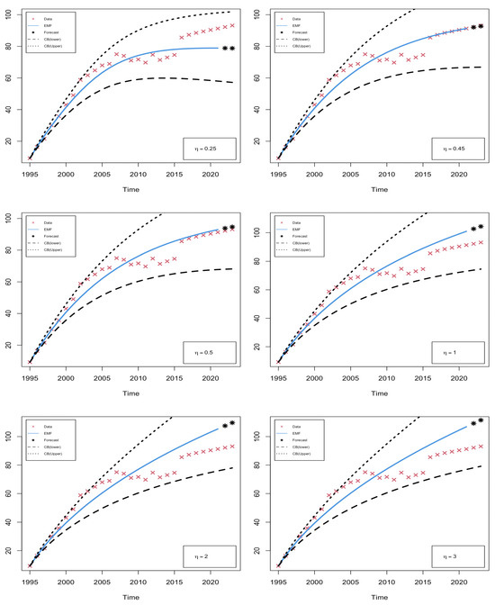
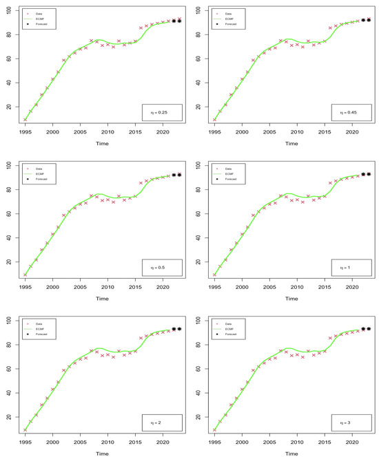
Since Internet access services were provided in the United States by the private sector during the mid-1990s, the interconnected network has expanded rapidly, driving substantial innovation in information technology and across many fields that rely on this technology. This expansion facilitated the emergence of a wide range of online services and new business models, fundamentally transforming communication, commerce, and patterns of economic interactions in the digital era. Internet users (see definition in [27]) are defined as individuals who have used the Internet at least once, from any location, in the last three months. The Internet can be accessed via a computer, mobile phone, personal digital assistant, game console, digital TV, or any other digital device. The proposed model is applied to analyze data on the percentage of individuals using the Internet in the United States during the years 1995–2023. Using data from 1995 to 2021, we train the model and estimate its parameters $\widehat{a}$, $\widehat{b}$, and $\widehat{\sigma }$ for different powers ($\eta =0.25, 0.45, 0.5, 1, 2$ and $\eta =3$). The result of this are summarized in Table 2. To forecast individuals using the Internet (% of population) in the United States for 2022 and 2023, we apply EMF and ECMF, replacing the estimated parameters into (13) and (12), respectively; see Table 3, Table 4, Table 5, Table 6, Table 7 and Table 8. Figure 1 displays the performance for our forecasts, the observed data, the EMF, and estimated confidence bands (CBs), illustrating how well the $\eta$-SLLDP fits the current data and makes accurate predictions. Figure 2 also displays the observed data, forecasts, and the ECMF.

Table 2. Estimation of the parameters for different powers.

$\mathit{\eta }$	$\widehat{\mathit{a}}$	$\widehat{\mathit{b}}$	$\widehat{\mathit{\sigma }}$
0.25	0.0001198147	0.0327607058	0.1895929565
0.45	0.003881824	0.147347894	0.107498178
0.5	0.006016280	0.17725340	0.09714150
1	0.045767700	0.40281507	0.04969654
2	0.156714130	0.60285514	0.02516242
3	0.275124390	0.68889513	0.01684088

Table 3. Predictions EMF and ECMF of the process for $\eta =0.25$.

Year	Real Data	EMF	ECMF
2022	92.2016	78.84276	91.21958
2023	93.1444	78.76999	92.1165

Table 4. Predictions EMF and ECMF of the process for $\eta =0.45$.

Year	Real Data	EMF	ECMF
2022	92.2016	92.01181	92.03106
2023	93.1444	92.70836	92.89958

Table 5. Predictions EMF and ECMF of the process for $\eta =0.5$.

Year	Real Data	EMF	ECMF
2022	92.2016	93.84579	92.1692
2023	93.1444	94.69541	93.03634

Table 6. Predictions EMF and ECMF of the process for $\eta =1$.

Year	Real Data	EMF	ECMF
2022	92.2016	102.7004	92.8443
2023	93.1444	104.3839	93.71301

Table 7. Predictions EMF and ECMF of the process for $\eta =2$.

Year	Real Data	EMF	ECMF
2022	92.2016	107.5801	93.17316
2023	93.1444	109.7306	94.04473

Table 8. Predictions EMF and ECMF of the process for $\eta =3$.

Year	Real Data	EMF	ECMF
2022	92.2016	109.2689	93.27471
2023	93.1444	111.5745	94.14707

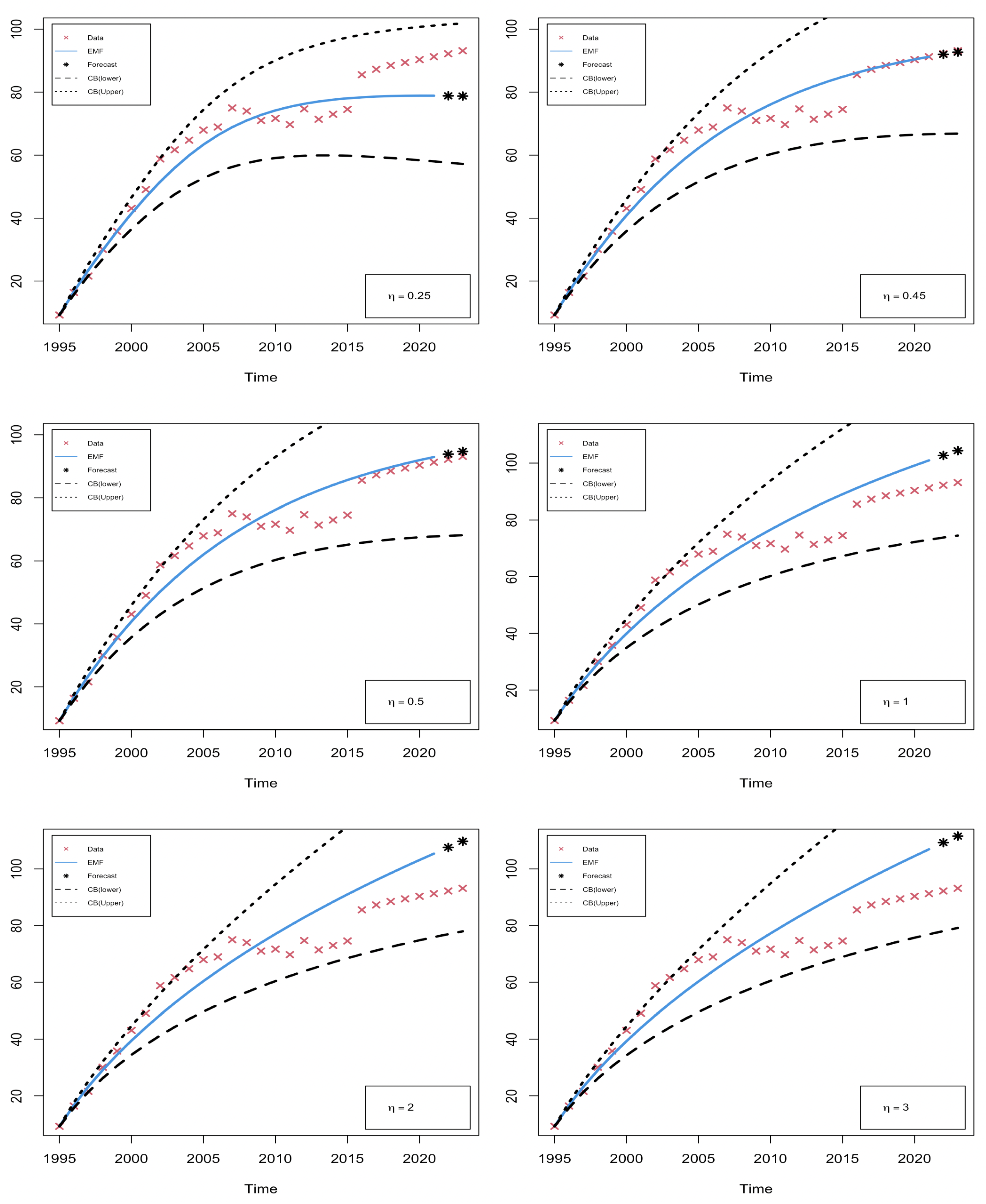
Figure 1. Real data, EMF, CB (lower), CB (upper), and the forecasted values.

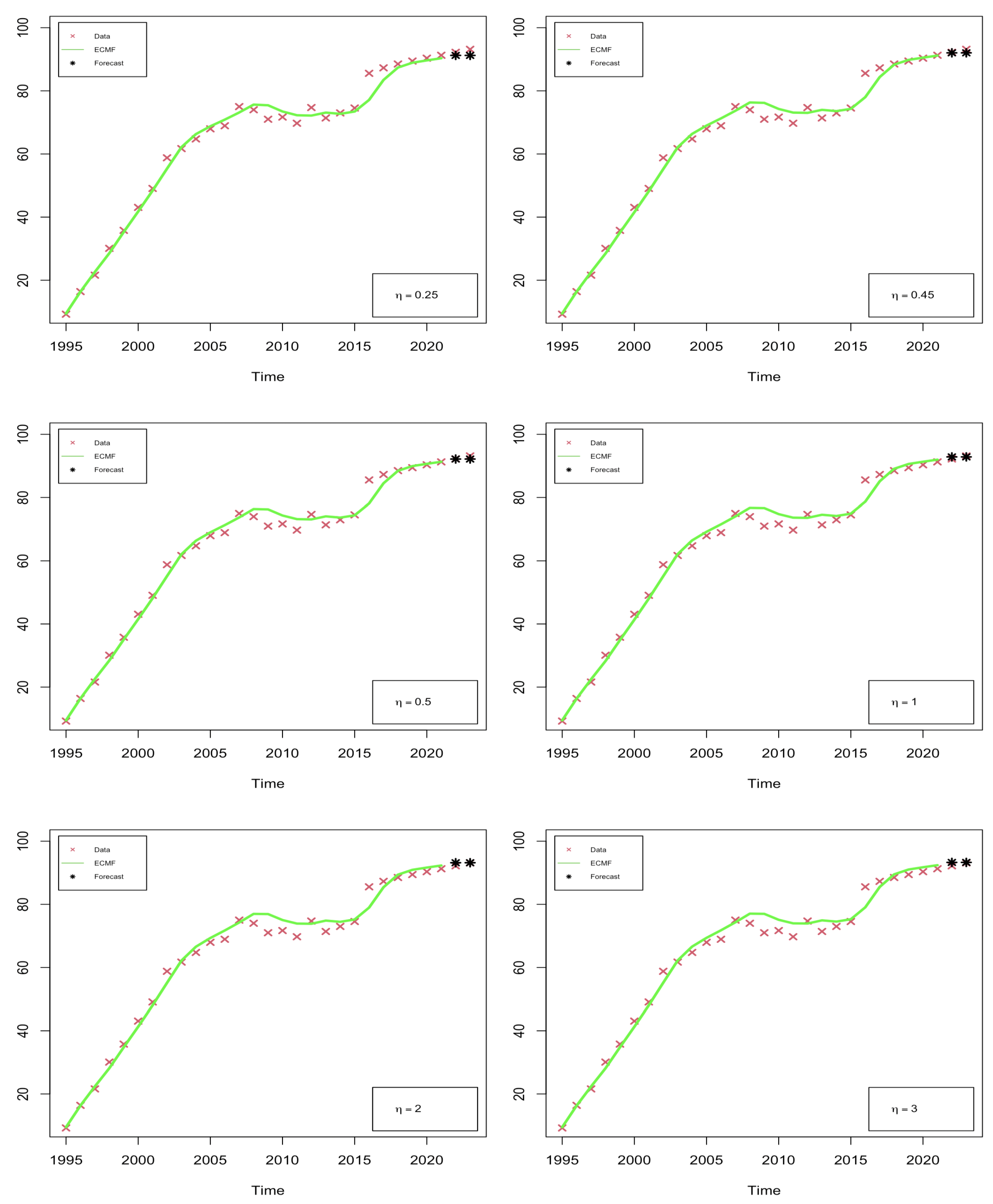
Figure 2. Real data, ECMF, and the forecasted values.

6.1.2. Goodness of Fit Analysis and Model Validation

Consider the observed data as $x\left(t_i\right)$, the mean of the real data $\overline{x}$, and the predicted data $\widehat{x}\left(t_i\right)$, which is obtained by substituting the estimated parameters in Equation (17). Let the error $e_i$ be defined as $e_i=x\left(t_i\right)-\widehat{x}\left(t_i\right)$, and let $\overline{e}$ be the mean of the errors (residuals). Over the years 1995–2021, for various values of $\eta$ ($\eta =0.25, 0.45, 0.5, 1, 2$ and $\eta =3$), the estimated parameters are calculated; the results are shown in Table 2. A global descriptive measure of the goodness of fit (GOF) between the adjusted values and the real data is calculated using the sampling variance as follows:

$$\begin{array}{cc}\hfill \mathrm{GOF}& =\left(1-{\displaystyle \frac{Var\left(e\right)}{Var\left(x\right)}}\right)\times 100\%,\hfill \end{array}$$

where the variance of error $Var\left(e\right)$ and the sampling variance of the real data $Var\left(x\right)$ are defined by

$$\begin{array}{cc}\hfill Var\left(e\right)& ={\displaystyle \frac{1}{27}}\sum _{i=1}^{27}{(e_i-\overline{e})}^2,\hfill \\ \hfill Var\left(x\right)& ={\displaystyle \frac{1}{27}}\sum _{i=1}^{27}{(x\left(t_i\right)-\overline{x})}^2.\hfill \end{array}$$

Table 9 shows the values obtained for GOF. In the case of $\eta =0.45$, we obtained the greatest value $94.94235\%$, while in the case of $\eta =1$, the GOF was $90.32621\%$. Thus, the inclusion of a power in the process improves the fit of real data.

Table 9. Goodness of fit (GOF) measures for the $\eta$-SLLDP model.

$\mathit{\eta }$	GOF
0.25	94.80362%
0.45	94.94235%
0.5	94.45417%
1	90.32621%
2	86.77910%
3	85.34479%

6.1.3. A Comparison of $\eta$-SLLDP and $\gamma$-SLKDP Models

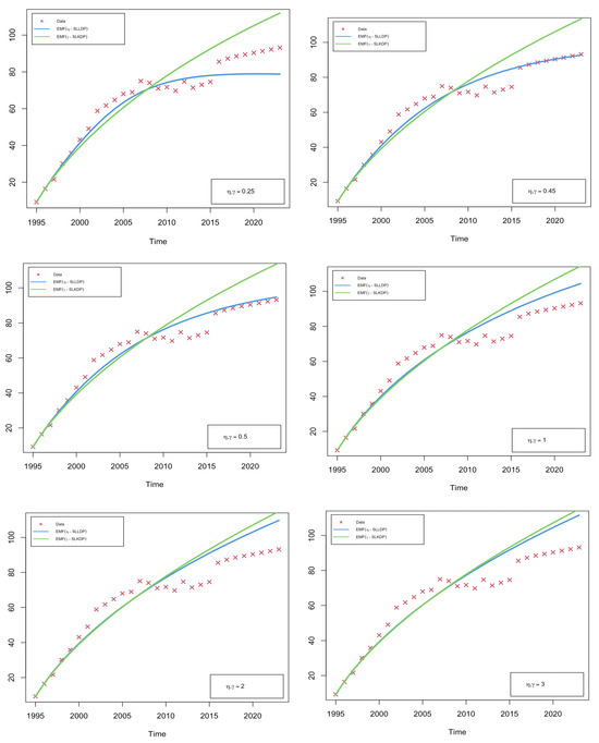
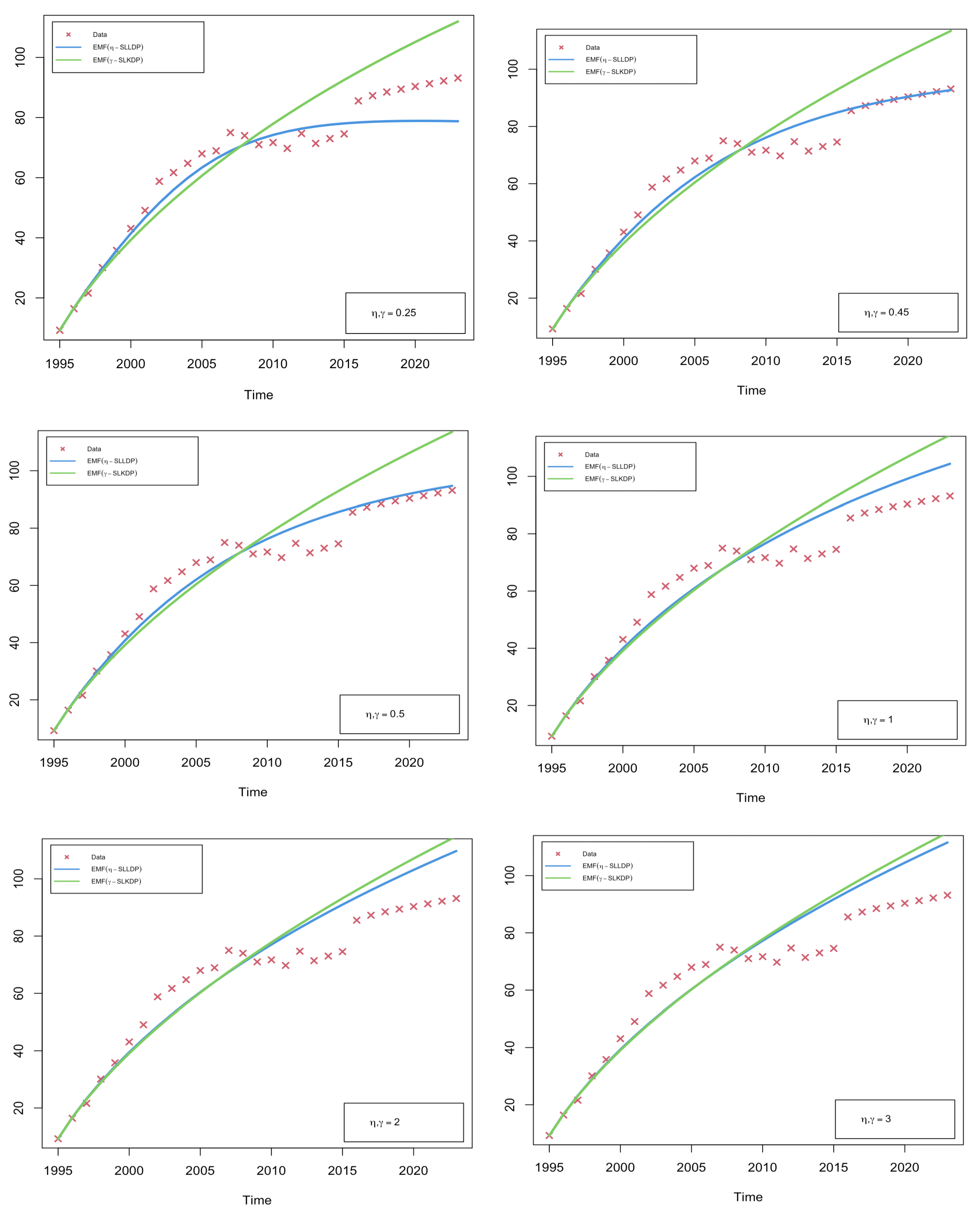
Here, the primary goal is to compare $\eta$-SLLDP and $\gamma$-SLKDP [21] models using the same real data set as in Table 1, where goodness of fit serves as the main evaluation criterion. Table 10 presents the estimated parameters for $\gamma$-SLKDP. Table 11 presents the GOF criterion, showing that the $\eta$-SLLDP has higher GOF values for all powers and thus surpasses the $\gamma$-SLKDP. Moreover, Figure 3 displays the fitted results obtained using the two models considered in this subsubsection, revealing that the $\eta$-SLLDP provides a better fit than the $\gamma$-SLKDP for the considered data set.

Table 10. Estimation of the parameters for $\gamma$-SLKDP.

$\mathit{\gamma }$	$\widehat{\mathit{\alpha }}$	$\widehat{\mathit{\beta }}$	$\widehat{\mathit{\sigma }}$
0.25	0.0757559	46.2440022	0.2033866
0.45	0.08946717	21.79842825	0.11306192
0.5	0.09120175	19.25044596	0.10176121
1	0.09906184	8.87192529	0.05088960
2	0.10302428	4.26787766	0.02544618
3	0.10434971	2.80966881	0.01696453

Table 11. Goodness of fit (GOF) measures for the $\eta$-SLLDP and $\gamma$-SLKDP models.

Power	GOF ($\mathit{\eta }$-SLLDP)	GOF ($\mathit{\gamma }$-SLKDP)
0.25	94.80362%	84.60053%
0.45	94.94235%	83.56693%
0.5	94.45417%	83.42953%
1	90.32621%	82.7875%
2	86.77910%	82.4515%
3	85.34479%	82.33713%

Figure 3. Observed data; EMF using $\eta$-SLLDP and $\gamma$-SLKDP.

6.2. Numerical Computations

In this subsection, numerical simulations are conducted to illustrate the dynamic behavior and numerical stability of the proposed $\eta$-SLLDP. The simulations are performed using the parameter estimates obtained from the real data application presented in Section 6.1. To investigate the effect of the power parameter, the simulations are carried out for several values of $\eta$, namely ($\eta =0.25, 0.45, 0.5, 1, 2$ and $\eta =3$).

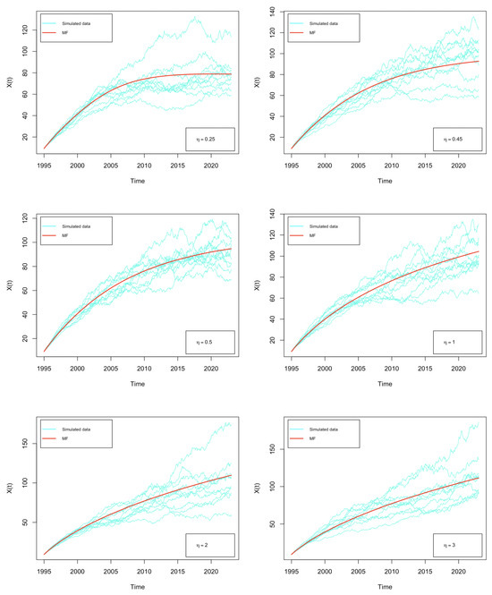
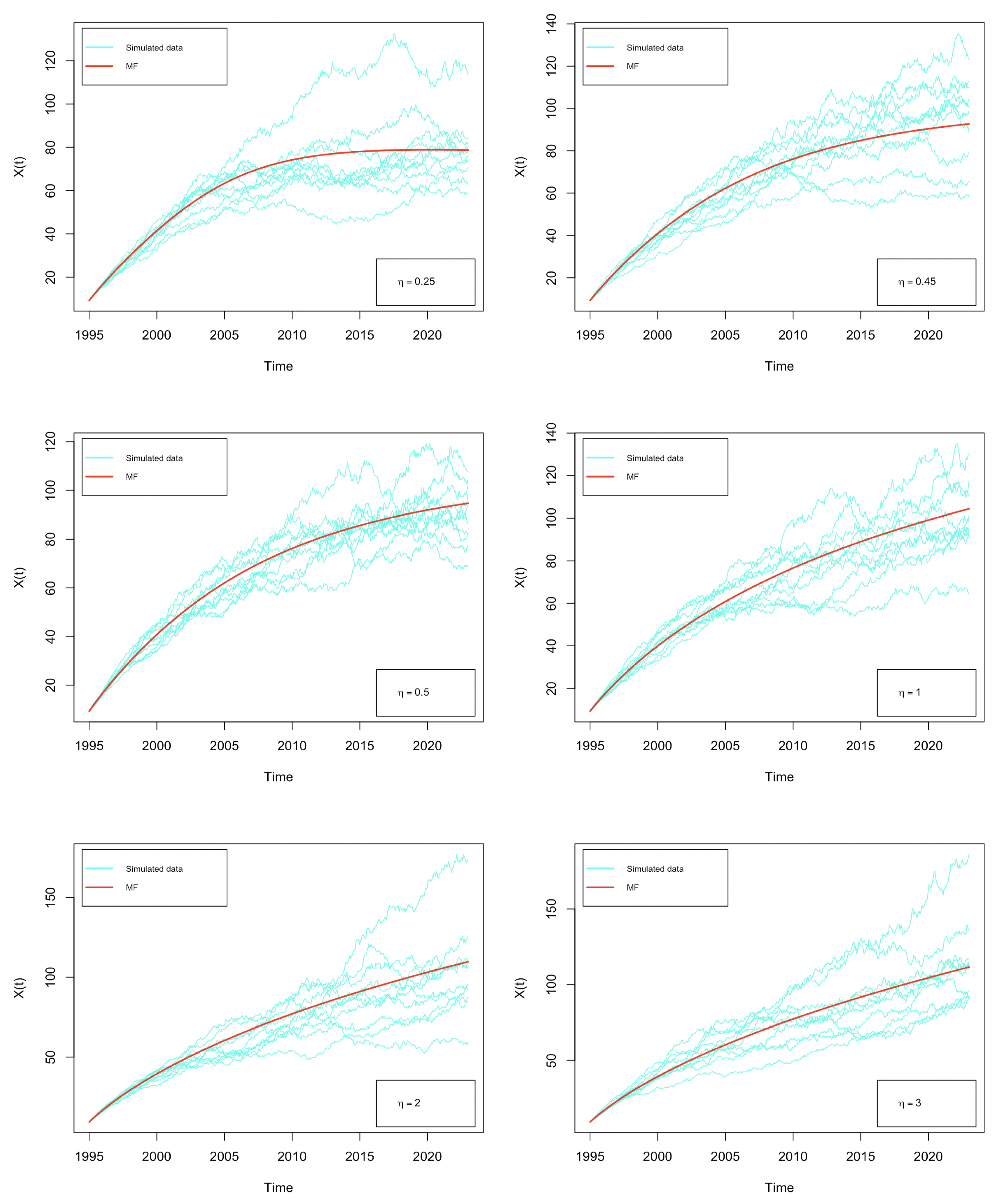
Ten sample trajectories, each containing 500 values, of the power stochastic log-logistic diffusion process are simulated using Equation (9) with a discretization step of $h=0.056$, $t_1=1995$, and the initial value $x_{t_1}=9.24$. The procedure used in this simulation is summarized in Algorithm 1. Figure 4 shows the simulated trajectories of the $\eta$-SLLDP versus MF for the values shown in Table 2.

Algorithm 1 Algorithm for simulating $\eta$-SLLDP sample trajectories.

1. Initialize, $t_1,T,N,x_1,a,b,\sigma ,\eta$. 2. Compute $\Delta :={\displaystyle \frac{T-t_1}{N}}$. 3. For $j=2,\dots ,N$, do (a) Discretize the time interval $[t_1,T]$ into N time points with each point computed as $t_j=t_{j-1}+(j-1)\Delta$; (b) Generate a standard normal observation, i.e., $Z_j\sim N(0,1)$, with the increments are computed as $W_j=W_{j-1}+\sqrt{\Delta }{Z}_j$; (c) The sample path of the $\eta$-SLLDP can be obtained upon using (9), i.e., $$X_j=X_{j-1}{\left({\displaystyle \frac{a+b^{\ln \left(t_{j-1}\right)}}{a+b^{\ln \left(t_j\right)}}}\right)}^{\eta }\exp \left(-{\displaystyle \frac{\eta {\sigma }^2}{2}}(t_j-t_{j-1})+\eta \sigma \left(W_j-W_{j-1}\right)\right).$$ 4. End do 5. Repeat Step 3 m times to obtain m sample paths.

Figure 4. Simulation along with the mean function.

7. Discussion

In this section, the figures and tables presented in the previous sections are discussed individually to interpret the numerical behavior and empirical findings of the proposed model.

Table 1 summarizes the percentage of individuals using the Internet in the United States over the period 1995–2023. The data reveal a strong upward trend, highlighting the continuous expansion of Internet accessibility and adoption over time. In the initial phase, the penetration rate increases rapidly from below 10% in 1995 to above 40% by the year 2000, indicating an accelerated diffusion of Internet technologies. During the subsequent years, the growth rate gradually moderates, with moderate fluctuations observed around the period 2007–2015. In the most recent years, the series approaches a saturation level exceeding 90%, reflecting a mature stage of technological adoption.

Table 2 reports the maximum likelihood estimates of the model parameters for different values of the power parameter $\eta$. The results indicate that the estimated parameters vary smoothly as $\eta$ changes, reflecting the flexibility of the proposed transformation in adapting the dynamics of the process. The stability of the estimates across a wide range of $\eta$ values suggests that the estimation procedure is numerically robust and does not exhibit erratic behavior. In particular, the diffusion parameter remains well-behaved, confirming the reliability of the stochastic component of the model.

Table 3, Table 4, Table 5, Table 6, Table 7 and Table 8 show that the estimated mean function varies with the choice of the parameter $\eta$. This behavior can be interpreted using the analytical expression of the mean function given in Equation (13), where $0<b<1$, which leads to ${\displaystyle \frac{a+\phi \left(t_1\right)}{a+\phi \left(t\right)}}>1$. For $0<\eta <1$, the exponent ${\displaystyle \frac{(\eta -1){\sigma }^2\eta }{2}}(t-t_1)$ is negative, so the exponential term remains below unity and introduces a moderating effect on the mean level. This moderating effect is less pronounced when $\eta$ is close to 0 or close to 1, and becomes stronger for intermediate values of $\eta$ (e.g., $\eta \approx 0.45$). For $\eta \ge 1$, the exponent is non-negative and increases with $\eta$, leading the exponential term to reach and exceed unity. In this case, the combined effect of the power and exponential components results in higher EMF values, which may contribute to overestimation relative to the observed data.

Figure 1 presents the real data together with the estimated mean function, confidence bands, and forecasted values for different values of the parameter $\eta$. The fitted curves closely track the observed trend, while most data points remain within the confidence bands, indicating reliable estimation and uncertainty assessment. The forecasted trajectories display smooth and stable behavior, supporting the predictive capability of the proposed model. Among the values considered, the best agreement with the observed data is obtained for intermediate values of $\eta$, particularly when $\eta$ is close to $0.45$. This behavior highlights the sensitivity of the fitted curves to the choice of $\eta$ and further demonstrates the flexibility of the proposed power transformation model.

Figure 2 displays the real observations together with the ECMF obtained from the fitted stochastic diffusion model for different values of the parameter $\eta$. The red crosses represent the observed data, while the green line corresponds to the estimated conditional mean function. It can be observed that, for all considered values of $\eta$, the ECMF accurately captures the global growth pattern and the saturation behavior of the process. The overall shape and long-term dynamics remain stable across different choices of $\eta$, which confirms the robustness of the estimation procedure and the adequacy of the proposed stochastic model for describing the underlying data dynamics.

Table 9 reports the GOF values for different values of $\eta$. The results show that the model performs best for intermediate values of the parameter $\eta$. The highest GOF is obtained at $\eta =0.45$ (94.94%), followed closely by $\eta =0.25$ and $\eta =0.5$. For $0<\eta <1$, the GOF values remain consistently high, suggesting that moderate attenuation induced by the $\eta$-power structure provides a balanced representation of the observed data. In particular, values of $\eta$ close to $0.45$ appear to offer an optimal compromise between under- and over-estimation. In contrast, when $\eta \ge 1$, the GOF decreases substantially as $\eta$ increases. This deterioration in fit reflects the increasingly rapid growth of the estimated mean function, which leads to systematic overestimation of the data. Overall, the results demonstrate that intermediate values of $\eta$ are more suitable for capturing the empirical dynamics, whereas larger values of $\eta$ result in poorer goodness-of-fit.

Table 10 reports the maximum likelihood estimates of the parameters for the $\gamma$-SLKDP model across different power values, showing that the scale and diffusion parameters decrease as the power increases, whereas the shape parameter increases slightly.

Figure 3 displays the fits made using the $\eta$-SLLDP and $\gamma$-SLKDP, revealing that the $\eta$-SLLDP performed much better than the $\gamma$-SLKDP in modeling the considered data set.

Table 11 presents the GOF criterion, showing that the $\eta$-SLLDP has higher GOF values for all powers and therefore outperforms the $\gamma$-SLKDP.

Figure 4 presents several Monte Carlo simulated sample paths generated from the fitted stochastic diffusion model, together with the mean function MF for different values of $\eta$ ( $\eta =0.25, 0.45, 0.5, 1, 2$ and $\eta =3$). The simulated paths exhibit increasing dispersion as time evolves, reflecting the cumulative effect of stochastic perturbations inherent in diffusion processes. At early stages, trajectories remain closely clustered around the MF, whereas variability gradually increases in later periods, which is consistent with theoretical properties of stochastic differential equations. In all cases, the MF is located approximately at the center of the simulated cloud of trajectories, indicating that the Monte Carlo simulations are correctly centered around the estimated deterministic trend. This confirms the internal consistency between parameter estimation, trend reconstruction, and numerical simulation. The overall qualitative behavior of the simulated dynamics remains stable, demonstrating the robustness of the model with respect to the choice of $\eta$.

8. Conclusions

This paper presented a study of the $\eta$-power stochastic log-logistic diffusion process, including all its probabilistic characteristics and statistical inference. The proposed model was applied to fit real data on individuals using the Internet (% of population) in the United States during the period 1995–2023. For different values of $\eta$ ($\eta =0.25,0.45,0.5,1,2$ and $\eta =3$), the parameter estimation was performed using the maximum likelihood method based on discrete sampling paths. Numerical procedures are employed to obtain the estimates. Furthermore, the EMF and the ECMF were computed. The capability of the $\eta$-SLLDP for forecasting and predicting was also examined. In addition, a global descriptive measure of the goodness of fit between the adjusted values and the real data was obtained using the sampling variance. The numerical results reported in Table 9 indicate that incorporating a power parameter into the proposed process leads to a notable improvement in goodness of fit, with the highest value 94.94235% at $\eta =0.45$, whereas for the classical case $\eta =1$ the corresponding value decreases to 90.32621%. This improvement is attributed to the additional flexibility introduced by the power structure, which allows the estimated mean function to avoid excessive damping or excessive growth, resulting in a closer fit to the observed data. Beyond the empirical application considered in this study, the flexible formulation of the model suggests potential applicability to other real-world data sets characterized by gradual stochastic dynamics and an overall increasing trend over time. Such applications may include technology adoption indicators (e.g., Internet usage), energy and environmental variables, population-related measures, and socio-economic indicators. Future research may further explore these application areas and assess the performance of the proposed model across different domains.

References

- Karatzas, I.; Shreve, S.E. Brownian Motion and Stochastic Calculus, 2nd ed.; Springer: New York, NY, USA, 1991. [Google Scholar] [CrossRef] [Scilit]
- Evans, L.C. An Introduction to Stochastic Differential Equations; American Mathematical Society: Providence, RI, USA, 2012. [Google Scholar] [CrossRef] [Scilit]
- Øksendal, B. Stochastic Differential Equations: An Introduction with Applications, 6th ed.; Springer: Berlin/Heidelberg, Germany, 2013. [Google Scholar] [CrossRef] [Scilit]
- Jacod, J.; Shiryaev, A.N. Limit Theorems for Stochastic Processes, 2nd ed.; Springer: Berlin/Heidelberg, Germany, 2002. [Google Scholar] [CrossRef] [Scilit]
- Mao, X. Stochastic Differential Equations and Applications, 2nd ed.; Elsevier: Amsterdam, The Netherlands, 2007. [Google Scholar]
- Sobczyk, K. Stochastic Differential Equations: With Applications to Physics and Engineering; Springer: Dordrecht, The Netherlands, 2001. [Google Scholar]
- El Azri, A.; Nafidi, A. A stochastic log-logistic diffusion process: Statistical computational aspects and application to real data. Stoch. Model. 2024, 40, 261–277. [Google Scholar] [CrossRef] [Scilit]
- Nafidi, A.; El Azri, A.; Gutiérrez-Sánchez, R. A Stochastic Schumacher Diffusion Process: Probability Characteristics Computation and Statistical Analysis. Methodol. Comput. Appl. Probab. 2023, 25, 66. [Google Scholar] [CrossRef] [Scilit]
- Nafidi, A.; Makroz, I.; Gutiérrez-Sánchez, R. A Stochastic Lomax Diffusion Process: Statistical Inference and Application. Mathematics 2021, 9, 100. [Google Scholar] [CrossRef] [Scilit]
- Nafidi, A.; Bahij, M.; Gutiérrez-Sánchez, R.; Achchab, B. Two-Parameter Stochastic Weibull Diffusion Model: Statistical Inference and Application to Real Modeling Example. Mathematics 2020, 8, 160. [Google Scholar] [CrossRef] [Scilit]
- Nafidi, A.; Moutabir, G.; Gutiérrez-Sánchez, R.; Ramos-Ábalos, E. Stochastic Square of the Brennan-Schwartz Diffusion Process: Statistical Computation and Application. Methodol. Comput. Appl. Probab. 2020, 7, 455–476. [Google Scholar] [CrossRef] [Scilit]
- Nafidi, A.; Moutabir, G.; Gutiérrez-Sánchez, R.; Achchab, B. Stochastic Brennan–Schwartz Diffusion Process: Statistical Computation and Application. Mathematics 2019, 7, 1062. [Google Scholar] [CrossRef] [Scilit]
- Gutiérrez, R.; Gutiérrez-Sánchez, R.; Nafidi, A. The trend of the total stock of the private car-petrol in Spain: Stochastic modelling using a new gamma diffusion process. Appl. Energy 2009, 86, 18–24. [Google Scholar] [CrossRef] [Scilit]
- Gutiérrez, R.; Gutiérrez-Sánchez, R.; Nafidi, A. Modelling and forecasting vehicle stocks using the trends of stochastic Gompertz diffusion models: The case of Spain. Appl. Stoch. Model. Bus. Ind. 2009, 25, 385–405. [Google Scholar] [CrossRef] [Scilit]
- Gutiérrez, R.; Gutiérrez-Sánchez, R.; Nafidi, A. The Stochastic Rayleigh diffusion model: Statistical inference and computational aspects. Applications to modelling of real cases. Appl. Math. Comput. 2006, 175, 628–644. [Google Scholar] [CrossRef] [Scilit]
- Nafidi, A.; El-Azri, A. A stochastic diffusion process based on the Lundqvist-Korf growth: Computational aspects and simulation. Math. Comput. Simul. 2021, 182, 25–38. [Google Scholar] [CrossRef] [Scilit]
- Alsheyab, S.; Shakhatreh, K. A new stochastic diffusion process based on generalized Gamma-like curve: Inference, computation, with applications. AIMS Math. 2024, 9, 27687–27703. [Google Scholar] [CrossRef] [Scilit]
- Alsheyab, S. A new stochastic diffusion process to model and predict electricity production from natural gas sources in the United States. Int. J. Appl. Math. 2025, 38, 1369–1388. [Google Scholar] [CrossRef] [Scilit]
- Chakroune, Y.; El Azri, A.; Nafidi, A. A τ-Power Stochastic Rayleigh Diffusion Model: Computational Aspects, Simulation and Predictive Analysis. Stochastics Qual. Control 2025, 40, 119–131. [Google Scholar] [CrossRef] [Scilit]
- Gutiérrez, R.; Gutiérrez-Sánchez, R.; Nafidi, A.; Ramos-Ábalos, E. A τ-power stochastic gamma diffusion process: Computational statistical inference and simulation aspects. A real example. Appl. Math. Comput. 2012, 219, 1576–1588. [Google Scholar] [CrossRef] [Scilit]
- El Azri, A.; Nafidi, A. A γ-power stochastic Lundqvist-Korf diffusion process: Computational aspects and simulation. Moroc. J. Pure Appl. Anal. 2022, 8, 364–374. [Google Scholar] [CrossRef] [Scilit]
- Kloeden, P.E.; Platen, E. Numerical Solution of Stochastic Differential Equations; Springer: Berlin/Heidelberg, Germany, 1992. [Google Scholar] [CrossRef] [Scilit]
- Zehna, P.W. Invariance of maximum likelihood estimators. Ann. Math. Stat. 1966, 37, 744–747. [Google Scholar] [CrossRef] [Scilit]
- Schervish, M.J. Theory of Statistics; Springer: New York, NY, USA, 1999. [Google Scholar] [CrossRef] [Scilit]
- Katsamaki, A.; Skiadas, C.H. Analytic solution and estimation of parameters on a stochastic exponential model for a technological diffusion process. Appl. Stoch. Models Data Anal. 1995, 11, 59–75. [Google Scholar] [CrossRef] [Scilit]
- R Core Team. R: A Language and Environment for Statistical Computing; R Foundation for Statistical Computing: Vienna, Austria, 2016; Available online: https://www.R-project.org/ (accessed on 3 December 2025).
- International Telecommunication Union (ITU). Individuals Using the Internet (% of Population). World Development Indicators (WDI), World Bank. 2025. Available online: https://databank.worldbank.org/source/world-development-indicators (accessed on 3 December 2025).
Disclaimer/Publisher’s Note: The statements, opinions and data contained in all publications are solely those of the individual author(s) and contributor(s) and not of MDPI and/or the editor(s). MDPI and/or the editor(s) disclaim responsibility for any injury to people or property resulting from any ideas, methods, instructions or products referred to in the content. |
© 2026 by the author. Licensee MDPI, Basel, Switzerland. This article is an open access article distributed under the terms and conditions of the Creative Commons Attribution (CC BY) license.