Article

A New Modification of Baskakov–Schurer–Stancu Operators: Weighted and Pointwise Approximation Theories


1
Department of Mathematics, Graduate of Natural and Applied Sciences, Gazi University, Beşevler, Ankara 06500, Türkiye
2
Department of Mathematics, College of Science, Qassim University, Saudi Arabia
3
Department of Mathematics, University Center for Research and Development, Chandigarh University, Mohali 140413, Punjab, India
4
Department of Mathematics, Van Yuzuncu Yil University, Van 65080, Türkiye
*
Author to whom correspondence should be addressed.
Mathematics 2026, 14(2), 241; https://doi.org/10.3390/math14020241
Submission received: 8 December 2025 / Revised: 27 December 2025 / Accepted: 4 January 2026 / Published: 8 January 2026

Abstract

The behavior of a new modification of operators of the Baskakov–Schurer–Stancu variant is discussed in this study. First, we establish certain necessary moment and central moment estimates. We then demonstrate the weighted approximation result of the suggested operators using a Korovkin-type theorem in weighted spaces. We also give the rate at which these operators converge. Next, we establish theorems of pointwise convergence. Finally, we show several graphical representations to illustrate the accuracy and functionality of the operators.

1. Introduction

A key component of mathematical analysis, approximation theory provides methodical ways to represent functions using more manageable and straightforward forms. The family of Bernstein polynomials, which S. N. Bernstein established in 1912 as part of his constructive demonstration of the Stone–Weierstrass theorem [1], is a fundamental concept in this discipline. Bernstein polynomials provide a reliable and easily understandable foundation for uniform approximation because of their positivity, continuity, and capacity to replicate endpoint values on the interval [ 0 , 1 ] . They are a common tool in the analysis of approximation processes because of their straightforward algebraic form and computational stability. Beyond their inherent theoretical value, Bernstein-type constructions represent more general topics in approximation theory, which has many uses in computational mathematics, signal processing, numerical analysis, and data fitting. Modern algorithms that need both accuracy and processing economy are based on techniques based on polynomials, splines, wavelets, and kernel approximations.
In [2], Schurer introduced a novel adaptation of Bernstein polynomials for ρ N { 0 } , Υ C [ 0 , 1 + ρ ] and ζ [ 0 , 1 ] as follows:
S ξ , ρ ( Υ ; ζ ) = σ = 0 ξ + ρ Υ σ ξ ξ + ρ σ ζ σ ( 1 ζ ) ξ + ρ σ .
Stancu [3] made a proposal in 1969 for ξ N the operators S ξ ϑ , ψ : C [ 0 , 1 ] C [ 0 , 1 ] , real parameters ϑ , ψ which are satisfied 0 ϑ ψ as below:
S ξ ϑ , ψ ( Υ ; ζ ) = σ = 0 ξ p ξ , σ ( ζ ) Υ σ + ϑ ξ + ψ ,
where the Bernstein basis functions defined by p ξ , σ ( ζ ) = ξ σ ζ σ ( 1 ζ ) ξ σ .
It should be noted that Stancu-type operators reduce to the well-known Bernstein operators explored by S. N. Bernstein [1] in 1912 when ϑ = 0 = ψ .
Inspired by the operator sequences mentioned above, many researchers have studied the results of various approximations in detail by creating modifications or generalizations of many different operator sequences. To gain a deeper understanding of this topic, numerous academic studies provide significant analyses and advancements; see [4,5,6,7,8,9,10,11,12,13,14]. These works examine the shape parameters extensively and offer detailed perspectives, practical applications in geometric modeling, and several new conceptual developments. Very recently, a novel class of Bernstein operators was derived by Usta [15] for Υ on C ( ( 0 , 1 ) ) , ξ N and ζ ( 0 , 1 ) as below:
S ξ * Υ ; ζ = 1 ξ σ = 0 ξ ξ σ ( σ ξ ζ ) 2 ζ σ 1 ( 1 ζ ) ξ σ 1 Υ σ ξ .
For Υ C [ 0 , ) , ζ ( 0 , ) and ξ N + , Cheng et al. [16] proposed and investigated the following new modification of the Baskakov-type [17] operators:
V ξ ( Υ ; ζ ) = 1 ξ σ = 0 ξ + σ 1 σ ζ σ 1 ( 1 + ζ ) ξ + σ + 1 ( ξ ζ σ ) 2 Υ σ ξ .
Motivated by [15,16], we aim to study the following new modification of Baskakov–Schurer–Stancu operators.
Let ρ 0 be a fixed positive integer and ϑ , ψ R with 0 ϑ ψ . For every function Υ C ( 0 , ) , the corresponding Baskakov–Schurer–Stancu operators are constructed as follows:
V ξ , ρ ϑ , ψ ( Υ ; ζ ) = 1 ξ + ρ σ = 0 v ξ , ρ , σ ( ζ ) ( ξ + ρ ) ζ σ 2 Υ σ + ϑ ξ + ψ ,
where
v ξ , ρ , σ ( ζ ) = ξ + ρ + σ 1 σ ζ σ 1 ( 1 + ζ ) ξ + ρ + σ + 1 .
Note that, when ϑ = ρ = ψ = 0 , operators V ξ , ρ ϑ , ψ reduce to the operators V ξ , which are constructed by Cheng et al. [16].
The layout of the paper is structured as follows: In Section 2, we present several essential moment calculations. Section 3 is devoted to the study of weighted approximation properties. In Section 4, we establish the rate of convergence of the proposed operators V ξ , ρ ϑ , ψ by means of the weighted modulus of continuity. Subsequently, Section 5 provides a collection of pointwise approximation results together with certain direct local theorems. In Section 6, we derive a Voronovskaja-type theorem. Lastly, Section 7 includes various graphical illustrations based on different parameter choices in order to show the accuracy and performance of the operators V ξ , ρ ϑ , ψ .

2. Preliminaries

We begin our analysis in this section by examining basic estimates pertaining to moments and central moments, which are essential for determining the primary findings.
Lemma 1.
Let σ = 0 σ m v ξ , ρ , σ ( ζ ) be a series of v ξ , ρ , σ base functions defined in (1). Here, σ m represents the power of the summation index and is used to compute the test functions in Lemma 2. The cases m = 0 , 1 , 2 , 3 , 4 are considered separately.
σ = 0 σ 0 v ξ , ρ , σ ( ζ ) = 1 ζ ( 1 + ζ ) , σ = 0 σ 1 v ξ , ρ , σ ( ζ ) = ξ + ρ 1 + ζ , σ = 0 σ 2 v ξ , ρ , σ ( ζ ) = ( ξ + ρ + 1 ) ( ξ + ρ ) ζ 1 + ζ + ξ + ρ 1 + ζ , σ = 0 σ 3 v ξ , ρ , σ ( ζ ) = ( ξ + ρ + 2 ) ( ξ + ρ + 1 ) ( ξ + ρ ) ζ 2 1 + ζ + 3 ( ξ + ρ + 1 ) ( ξ + ρ ) ζ 1 + ζ + ξ + ρ 1 + ζ , σ = 0 σ 4 v ξ , ρ , σ ( ζ ) = ( ξ + ρ + 3 ) ( ξ + ρ + 2 ) ( ξ + ρ + 1 ) ( ξ + ρ ) ζ 3 1 + ζ + 6 ( ξ + ρ + 2 ) ( ξ + ρ + 1 ) ( ξ + ρ ) ζ 2 1 + ζ + 7 ( ξ + ρ + 1 ) ( ξ + ρ ) ζ 1 + ζ + ξ + ρ 1 + ζ .
Proof. 
Using the negative binomial series σ = 0 n + σ 1 σ z σ = ( 1 z ) n , | z | 1 with n = ξ + ρ and z = ζ 1 + ζ , and multiplying by the factor ( 1 ζ ) ( ξ + ρ ) , we obtain that the above series equals 1.
σ = 0 σ 0 v ξ , ρ , σ ( ζ ) = σ = 0 σ 0 ξ + ρ + σ 1 σ ζ σ 1 ( 1 + ζ ) ξ + ρ + σ + 1 = 1 ζ ( 1 + ζ ) σ = 0 σ 0 ξ + ρ + σ 1 σ ζ σ ( 1 + ζ ) ξ + ρ + σ = 1 ζ ( 1 + ζ ) .
σ = 0 σ 1 v ξ , ρ , σ ( ζ ) = σ = 1 σ 1 ξ + ρ + σ 1 σ ζ σ 1 ( 1 + ζ ) ξ + ρ + σ + 1 = 1 ζ ( 1 + ζ ) σ = 1 σ ξ + ρ + σ 1 σ ζ σ ( 1 + ζ ) ξ + ρ + σ .
When we substitute σ + 1 for σ in the equation above, we obtain
σ = 0 σ 1 v ξ , ρ , σ ( ζ ) = 1 ζ ( 1 + ζ ) σ = 0 ( σ + 1 ) ξ + ρ + σ σ + 1 ζ σ + 1 ( 1 + ζ ) ξ + ρ + σ + 1 .
Using ξ + ρ to multiply and divide the equation above, we get
σ = 0 σ 1 v ξ , ρ , σ ( ζ ) = ξ + ρ 1 + ζ σ = 0 ξ + ρ + σ σ ζ σ ( 1 + ζ ) ξ + ρ + σ + 1 = ξ + ρ 1 + ζ .
σ = 0 σ 2 v ξ , ρ , σ ( ζ ) = σ = 0 σ 2 ξ + ρ + σ 1 σ ζ σ 1 ( 1 + ζ ) ξ + ρ + σ + 1 = 1 ζ ( 1 + ζ ) σ = 0 σ 2 ξ + ρ + σ 1 σ ζ σ ( 1 + ζ ) ξ + ρ + σ .
By substituting σ ( σ 1 ) + σ for σ 2 , one has
σ = 0 σ 2 v ξ , ρ , σ ( ζ ) = 1 ζ ( 1 + ζ ) σ = 2 σ ( σ 1 ) ξ + ρ + σ 1 σ ζ σ ( 1 + ζ ) ξ + ρ + σ + 1 ζ ( 1 + ζ ) σ = 1 σ ξ + ρ + σ 1 σ ζ σ ( 1 + ζ ) ξ + ρ + σ .
When we substitute σ + 2 for σ in the first summation, we obtain
σ = 0 σ 2 v ξ , ρ , σ ( ζ ) = 1 ζ ( 1 + ζ ) σ = 0 ( σ + 2 ) ( σ + 1 ) ξ + ρ + σ + 1 σ + 2 ζ σ + 2 ( 1 + ζ ) ξ + ρ + σ + 2 + σ = 0 σ 1 v ξ , ρ , σ ( ζ ) .
Using ( ξ + ρ + 1 ) ( ξ + ρ ) to multiply and divide the first summation, we get
σ = 0 σ 2 v ξ , ρ , σ ( ζ ) = ( ξ + ρ + 1 ) ( ξ + ρ ) ζ 1 + ζ σ = 0 ξ + ρ + σ + 1 σ ζ σ ( 1 + ζ ) ξ + ρ + σ + 2 + ξ + ρ 1 + ζ = ( ξ + ρ + 1 ) ( ξ + ρ ) ζ 1 + ζ + ξ + ρ 1 + ζ .
The proof consists of five assertions. Assertions σ = 0 σ 0 v ξ , ρ , σ ( ζ ) , σ = 0 σ 1 v ξ , ρ , σ ( ζ ) and σ = 0 σ 2 v ξ , ρ , σ ( ζ ) are proved explicitly above. For the proof of assertion σ = 0 σ 3 v ξ , ρ , σ ( ζ ) , we replace σ 3 with σ ( σ 1 ) ( σ 2 ) + 3 σ ( σ 1 ) + σ . Similarly, for the proof of assertion σ = 0 σ 4 v ξ , ρ , σ ( ζ ) , we replace σ 4 with σ ( σ 1 ) ( σ 2 ) ( σ 3 ) + 6 σ ( σ 1 ) ( σ 2 ) + 7 σ ( σ 1 ) + σ . Once these substitutions are made, the proof can be completed in an analogous way. □
Lemma 2.
Let ρ 0 be a fixed positive integer, and ϑ , ψ R with 0 ϑ ψ . For every ζ ( 0 , ) , the operators V ξ , ρ ϑ , ψ satisfy
V ξ , ρ ϑ , ψ ( 1 ; ζ ) = 1 , V ξ , ρ ϑ , ψ ( ϱ ; ζ ) = ( ξ + ρ + 2 ) ζ ξ + ψ + ϑ + 1 ξ + ψ , V ξ , ρ ϑ , ψ ( ϱ 2 ; ζ ) = ( ξ + ρ ) 2 + 7 ( ξ + ρ ) + 6 ζ 2 ( ξ + ψ ) 2 + ( 2 ϑ + 5 ) ( ξ + ρ ) + 4 ϑ + 6 ζ ( ξ + ψ ) 2 + ( ϑ + 1 ) 2 ( ξ + ψ ) 2 , V ξ , ρ ϑ , ψ ( ϱ 3 ; ζ ) = ( ξ + ρ ) 3 + 15 ( ξ + ρ ) 2 + 38 ( ξ + ρ ) + 24 ζ 3 ( ξ + ψ ) 3 + ( 3 ϑ + 12 ) ( ξ + ρ ) 2 + ( 21 ϑ + 48 ) ( ξ + ρ ) + 18 ϑ + 36 ζ 2 ( ξ + ψ ) 3 + ( 3 ϑ 2 + 15 ϑ + 13 ) ( ξ + ρ ) + 6 ϑ 2 + 18 ϑ + 14 ζ ( ξ + ψ ) 3 + ( ϑ + 1 ) 3 ( ξ + ψ ) 3 ,
V ξ , ρ ϑ , ψ ( ϱ 4 ; ζ ) = ( ξ + ρ ) 4 + 26 ( ξ + ρ ) 3 + 131 ( ξ + ρ ) 2 + 226 ( ξ + ρ ) + 120 ζ 4 ( ξ + ψ ) 4 + ( 4 ϑ + 22 ) ( ξ + ρ ) 3 + ( 60 ϑ + 186 ) ( ξ + ρ ) 2 + ( 152 ϑ + 404 ) ( ξ + ρ ) + 96 ϑ + 240 ζ 3 ( ξ + ψ ) 4 + ( 6 ϑ 2 + 48 ϑ + 61 ) ( ξ + ρ ) 2 + ( 42 ϑ 2 + 48 ϑ + 211 ) ( ξ + ρ ) + 144 ϑ + 150 ζ 2 ( ξ + ψ ) 4 + ( 4 ϑ 3 + 30 ϑ 2 + 52 ϑ + 29 ) ( ξ + ρ ) + 8 ϑ 3 + 26 ϑ 2 + 56 ϑ + 30 ζ ( ξ + ψ ) 4 + ( ϑ + 1 ) 4 ( ξ + ψ ) 4 .
Proof. 
From Lemma 1, we arrive at
V ξ , ρ ϑ , ψ ( 1 ; ζ ) = 1 ξ + ρ σ = 0 ξ + ρ + σ 1 σ ζ σ 1 ( 1 + ζ ) ξ + ρ + σ + 1 ( ξ + ρ ) ζ σ 2 = 1 ξ + ρ σ = 0 ξ + ρ + σ 1 σ ζ σ 1 ( 1 + ζ ) ξ + ρ + σ + 1 ( ξ + ρ ) 2 ζ 2 2 ( ξ + ρ ) ζ σ + σ 2 = ( ξ + ρ ) 2 ζ 2 ξ + ρ σ = 0 ξ + ρ + σ 1 σ ζ σ 1 ( 1 + ζ ) ξ + ρ + σ + 1 2 ( ξ + ρ ) ζ ξ + ρ σ = 0 σ ξ + ρ + σ 1 σ ζ σ 1 ( 1 + ζ ) ξ + ρ + σ + 1 + 1 ξ + ρ σ = 0 σ 2 ξ + ρ + σ 1 σ ζ σ 1 ( 1 + ζ ) ξ + ρ + σ + 1 = ( ξ + ρ ) 2 ζ 2 ξ + ρ 1 ζ ( 1 + ζ ) 2 ( ξ + ρ ) ζ ξ + ρ ξ + ρ 1 + ζ + 1 ξ + ρ ( ξ + ρ + 1 ) ( ξ + ρ ) ζ 1 + ζ + ξ + ρ 1 + ζ = ( ξ + ρ ) ζ ( 1 + ζ ) 2 ( ξ + ρ ) ζ ( 1 + ζ ) + ( ξ + ρ + 1 ) ζ 1 + ζ + 1 1 + ζ = ( ξ + ρ 2 ξ 2 ρ + ξ + ρ + 1 ) ζ ( 1 + ζ ) + 1 1 + ζ = 1 + ζ 1 + ζ = 1 .
V ξ , ρ ϑ , ψ ( ϱ ; ζ ) = 1 ξ + ρ σ = 0 ξ + ρ + σ 1 σ ζ σ 1 ( 1 + ζ ) ξ + ρ + σ + 1 ( ξ + ρ ) ζ σ 2 σ + ϑ ξ + ψ = 1 ( ξ + ρ ) ( ξ + ψ ) σ = 0 ξ + ρ + σ 1 σ ζ σ 1 ( 1 + ζ ) ξ + ρ + σ + 1 ( ξ + ρ ) ζ σ 2 σ + ϑ ξ + ψ = 1 ( ξ + ρ ) ( ξ + ψ ) σ = 0 ξ + ρ + σ 1 σ ζ σ 1 ( 1 + ζ ) ξ + ρ + σ + 1 ( ξ + ρ ) 2 ζ 2 σ 2 ( ξ + ρ ) ζ σ 2 + σ 3 + ϑ ξ + ψ = ( ξ + ρ ) 2 ζ 2 ( ξ + ρ ) ( ξ + ψ ) σ = 0 σ ξ + ρ + σ 1 σ ζ σ 1 ( 1 + ζ ) ξ + ρ + σ + 1 2 ( ξ + ρ ) ζ ( ξ + ρ ) ( ξ + ψ ) σ = 0 σ 2 ξ + ρ + σ 1 σ ζ σ 1 ( 1 + ζ ) ξ + ρ + σ + 1 + 1 ( ξ + ρ ) ( ξ + ψ ) σ = 0 σ 3 ξ + ρ + σ 1 σ ζ σ 1 ( 1 + ζ ) ξ + ρ + σ + 1 + ϑ ξ + ψ = ( ξ + ρ ) 2 ζ 2 ( ξ + ρ ) ( ξ + ψ ) ξ + ρ 1 + ζ
2 ( ξ + ρ ) ζ ( ξ + ρ ) ( ξ + ψ ) ( ξ + ρ + 1 ) ( ξ + ρ ) ζ 1 + ζ + ξ + ρ 1 + ζ + 1 ( ξ + ρ ) ( ξ + ψ ) ( ξ + ρ + 2 ) ( ξ + ρ + 1 ) ( ξ + ρ ) ζ 2 1 + ζ + 3 ( ξ + ρ + 1 ) ( ξ + ρ ) ζ 1 + ζ + ξ + ρ 1 + ζ + ϑ ξ + ψ = ( ξ + ρ ) 2 ζ 2 ( ξ + ψ ) ( 1 + ζ ) 2 ( ξ + ρ + 1 ) ( ξ + ρ ) ζ 2 ( ξ + ψ ) ( 1 + ζ ) 2 ( ξ + ρ ) ζ ( ξ + ψ ) ( 1 + ζ ) + ( ξ + ρ + 2 ) ( ξ + ρ + 1 ) ζ 2 ( ξ + ψ ) ( 1 + ζ ) + 3 ( ξ + ρ + 1 ) ζ ( ξ + ψ ) ( 1 + ζ ) + 1 ( ξ + ψ ) ( 1 + ζ ) + ϑ ξ + ψ = ξ ζ 2 + ξ ζ + ρ ζ 2 + ρ ζ + 2 ζ 2 + 2 ζ + ζ + 1 ( ξ + ψ ) ( 1 + ζ ) + ϑ ξ + ψ = ξ ζ ( 1 + ζ ) + ρ ζ ( 1 + ζ ) + 2 ζ ( 1 + ζ ) + 1 + ζ ( ξ + ψ ) ( 1 + ζ ) + ϑ ξ + ψ = ( ξ ζ + ρ ζ + 2 ζ + 1 ) ( 1 + ζ ) ( ξ + ψ ) ( 1 + ζ ) + ϑ ξ + ψ = ( ξ + ρ + 2 ) ζ ξ + ψ + ϑ + 1 ξ + ψ .
V ξ , ρ ϑ , ψ ( ϱ 2 ; ζ ) = 1 ξ + ρ σ = 0 ξ + ρ + σ 1 σ ζ σ 1 ( 1 + ζ ) ξ + ρ + σ + 1 ( ξ + ρ ) ζ σ 2 σ + ϑ ξ + ψ 2 = 1 ( ξ + ρ ) ξ + ψ 2 σ = 0 ξ + ρ + σ 1 σ ζ σ 1 ( 1 + ζ ) ξ + ρ + σ + 1 ( ξ + ρ ) ζ σ 2 ( σ + ϑ ) 2 = 1 ( ξ + ρ ) ξ + ψ 2 σ = 0 σ 4 ξ + ρ + σ 1 σ ζ σ 1 ( 1 + ζ ) ξ + ρ + σ + 1 + 2 ( ϑ ( ξ + ρ ) ζ ) ( ξ + ρ ) ξ + ψ 2 σ = 0 σ 3 ξ + ρ + σ 1 σ ζ σ 1 ( 1 + ζ ) ξ + ρ + σ + 1 + ( ξ + ρ ) 2 ζ 2 + ϑ 2 4 ϑ ( ξ + ρ ) ζ ( ξ + ρ ) ξ + ψ 2 σ = 0 σ 2 ξ + ρ + σ 1 σ ζ σ 1 ( 1 + ζ ) ξ + ρ + σ + 1 + 2 ϑ ( ξ + ρ ) 2 ζ 2 2 ϑ 2 ( ξ + ρ ) ζ ( ξ + ρ ) ξ + ψ 2 σ = 0 σ ξ + ρ + σ 1 σ ζ σ 1 ( 1 + ζ ) ξ + ρ + σ + 1 + ϑ 2 ( ξ + ρ ) 2 ζ 2 ( ξ + ρ ) ξ + ψ 2 σ = 0 ξ + ρ + σ 1 σ ζ σ 1 ( 1 + ζ ) ξ + ρ + σ + 1 = 1 ( ξ + ρ ) ξ + ψ 2 ( ( ξ + ρ + 3 ) ( ξ + ρ + 2 ) ( ξ + ρ + 1 ) ( ξ + ρ ) ζ 3 1 + ζ + 6 ( ξ + ρ + 2 ) ( ξ + ρ + 1 ) ( ξ + ρ ) ζ 2 1 + ζ + 7 ( ξ + ρ + 1 ) ( ξ + ρ ) ζ 1 + ζ + ξ + ρ 1 + ζ ) + 2 ( ϑ ( ξ + ρ ) ζ ) ( ξ + ρ ) ξ + ψ 2 ( ξ + ρ + 2 ) ( ξ + ρ + 1 ) ( ξ + ρ ) ζ 2 1 + ζ + 3 ( ξ + ρ + 1 ) ( ξ + ρ ) ζ 1 + ζ + ξ + ρ 1 + ζ + ( ξ + ρ ) 2 ζ 2 + ϑ 2 4 ϑ ( ξ + ρ ) ζ ( ξ + ρ ) ξ + ψ 2 ( ξ + ρ + 1 ) ( ξ + ρ ) ζ 1 + ζ + ξ + ρ 1 + ζ + 2 ϑ ( ξ + ρ ) 2 ζ 2 2 ϑ 2 ( ξ + ρ ) ζ ( ξ + ρ ) ξ + ψ 2 ξ + ρ 1 + ζ + ϑ 2 ( ξ + ρ ) 2 ζ 2 ( ξ + ρ ) ξ + ψ 2 1 ζ ( 1 + ζ ) = ( ξ + ρ ) 2 + 7 ( ξ + ρ ) + 6 ζ 2 ( ξ + ψ ) 2 + ( 2 ϑ + 5 ) ( ξ + ρ ) + 4 ϑ + 6 ζ ( ξ + ψ ) 2 + ( ϑ + 1 ) 2 ( ξ + ψ ) 2 .
Hence, we have established the proof equations V ξ , ρ ϑ , ψ ( 1 ; ζ ) , V ξ , ρ ϑ , ψ ( ϱ ; ζ ) and V ξ , ρ ϑ , ψ ( ϱ 2 ; ζ ) . In the same manner, the expressions for V ξ , ρ ϑ , ψ ( ϱ 3 ; ζ ) and V ξ , ρ ϑ , ψ ( ϱ 4 ; ζ ) can be derived directly. For this reason, we omit the detailed steps here. □
Lemma 3.
Let ρ 0 be a fixed positive integer, and ϑ , ψ R with 0 ϑ ψ . For every ζ ( 0 , ) , operators V ξ , ρ ϑ , ψ satisfy
V ξ , ρ ϑ , ψ ( ϱ ζ ; ζ ) = ( ρ ψ + 2 ) ζ ξ + ψ + ϑ + 1 ξ + ψ , V ξ , ρ ϑ , ψ ( ( ϱ ζ ) 2 ; ζ ) = ( ξ + ρ + 6 ) ( ξ + ρ + 1 ) 2 ( ξ + ρ + 2 ) ( ξ + ψ ) + ( ξ + ψ ) 2 ζ 2 ( ξ + ψ ) 2 + ( 2 ϑ + 5 ) ( ξ + ρ ) + 4 ϑ + 6 2 ( ϑ + 1 ) ( ξ + ψ ) ζ ( ξ + ψ ) 2 + ( ϑ + 1 ) 2 ( ξ + ψ ) 2 , V ξ , ρ ϑ , ψ ( ( ϱ ζ ) 4 ; ζ ) = ( ( ξ + ρ + 20 ) ( ξ + ρ + 3 ) ( ξ + ρ + 2 ) ( ξ + ρ + 1 ) ( ξ + ψ ) 4 4 ( ξ + ρ + 2 ) ( ξ + ρ + 1 ) ( ξ + ρ + 12 ) ( ξ + ψ ) ( ξ + ψ ) 4 + 6 ( ξ + ρ + 6 ) ( ξ + ρ + 1 ) ( ξ + ψ ) 2 ( ξ + ψ ) 4 4 ( ξ + ρ + 2 ) ( ξ + ψ ) 3 + ( ξ + ψ ) 4 ( ξ + ψ ) 4 ) ζ 4 + ( ( 4 ϑ + 22 ) ( ξ + ρ ) + 48 ϑ + 120 ( ξ + ρ + 1 ) ( ξ + ρ + 2 ) ( ξ + ψ ) 4 12 ( ϑ + 4 ) ( ξ + ρ ) + 6 ϑ + 12 ( ξ + ρ + 1 ) ( ξ + ψ ) ( ξ + ψ ) 4 + 6 ( 2 ϑ + 5 ) ( ξ + ρ ) + 4 ϑ + 6 ( ξ + ψ ) 2 4 ( ϑ + 1 ) ( ξ + ψ ) 3 ( ξ + ψ ) 4 ) ζ 3 + ( ( 6 ϑ 2 + 48 ϑ + 61 ) ( ξ + ρ ) + 36 ϑ 2 + 144 ϑ + 150 ( ξ + ρ + 1 ) ( ξ + ψ ) 4 4 ( 3 ϑ 2 + 15 ϑ + 13 ) ( ξ + ρ ) + 6 ϑ 2 + 18 ϑ + 14 ( ξ + ψ ) ( ξ + ψ ) 4 + 6 ( ϑ + 1 ) 2 ( ξ + ψ ) 2 ( ξ + ψ ) 4 ) ζ 2 + ( ( 4 ϑ + 30 ϑ 2 + 52 ϑ + 29 ) ( ξ + ρ ) + 8 ϑ 3 + 3 ϑ 2 + 56 ϑ + 30 ( ξ + ψ ) 4 4 ( ϑ + 1 ) 3 ( ξ + ψ ) ( ξ + ψ ) 4 ) ζ + ( ϑ + 1 ) 4 ( ξ + ψ ) 4 .
The proof follows from Lemma 2 and the linearity and positivity of V ξ , ρ ϑ , ψ .

3. Weighted Approximation of Operators V ξ , ρ ϑ , ψ

All functions on ( 0 , ) that satisfy the inequality | Υ ( ζ ) | S Υ ν ( ζ ) form the set B ν ( 0 , ) . Here, S Υ is a positive constant depending only on the function Υ and ν ( ζ ) = 1 + ζ 2 . Additionally, let us denote these spaces as follows:
C ν ( 0 , ) = B ν ( 0 , ) C ( 0 , )
and
C ν * ( 0 , ) = { Υ C ν ( 0 , ) : lim ξ Υ ( ζ ) ν ( ζ ) < }
and equipped with the norm
Υ ν = sup | Υ ( ζ ) | ν ( ζ ) : ζ ( 0 , ) .
Theorem 1.
For every Υ C ν * ( 0 , ) , we have
lim ξ V ξ , ρ ϑ , ψ ( Υ ) Υ ν = 0 .
Proof. 
It is sufficient to verify the following three requirements from [18,19,20,21].
lim ξ V ξ , ρ ϑ , ψ ( ϱ η ; ζ ) ζ η ν = 0 , η = 0 , 1 , 2 .
Since V ξ , ρ ϑ , ψ ( 1 ; ζ ) = 1 , condition (2) holds for η = 0 . The following inequality can be derived using Lemma 2.
V ξ , ρ ϑ , ψ ( ϱ ; ζ ) ζ ν sup ζ 0 ( ξ + ρ + 2 ) ζ ξ + ψ + ϑ + 1 ξ + ψ ζ 1 + ζ 2 = sup ζ 0 ( ρ ψ + 2 ) ζ ξ + ψ + ϑ + 1 ξ + ψ 1 + ζ 2 | ρ ψ + 2 | + ϑ + 1 ξ + ψ .
The condition in (2) is therefore satisfied to be true for η = 1 for lim ξ V ξ , ρ ϑ , ψ ( ϱ ; ζ ) ζ ν = 0 . Likewise, this can be analyzed using Lemma 2
V ξ , ρ ϑ , ψ ( ϱ 2 ; ζ ) ζ 2 ν sup ζ 0 ( ξ + ρ ) 2 + 7 ( ξ + ρ ) + 6 ζ 2 ( ξ + ψ ) 2 + ( 2 ϑ + 5 ) ( ξ + ρ ) + 4 ϑ + 6 ζ ( ξ + ψ ) 2 + ( ϑ + 1 ) 2 ( ξ + ψ ) 2 ζ 2 1 + ζ 2 = sup ζ 0 2 ( ρ ψ + 7 ) ξ + ρ 2 ψ 2 + 7 ρ + 6 ζ 2 ( ξ + ψ ) 2 + ( 2 ϑ + 5 ) ( ξ + ρ ) + 4 ϑ + 6 ζ ( ξ + ψ ) 2 + ( ϑ + 1 ) 2 ( ξ + ψ ) 2 1 + ζ 2 ( 2 | ρ ψ | + 7 ) ξ + ρ 2 + 7 ρ + 6 + ( 2 ϑ + 5 ) ( ξ + ρ ) + 4 ϑ + 6 + ( ϑ + 1 ) 2 ( ξ + ψ ) 2 .
Then, if lim ξ V ξ , ρ ϑ , ψ ( ϱ 2 ; ζ ) ζ 2 ν = 0 , it follows that condition (2) holds for η = 2 . Therefore, the assertion is proved. □

4. Rate of Convergence of Operators V ξ , ρ ϑ , ψ

Let
Ω ( Υ ; δ ) = sup ζ ( 0 , ) , | l | δ | Υ ( ζ + l ) Υ ( ζ ) | ( 1 + ζ 2 ) ( 1 + l 2 ) ,
for every Υ C ν * ( 0 , ) . The weighted modulus of continuity of the function Υ is defined by Ω ( Υ ; δ ) [22]. Moreover, the properties of Ω ( Υ ; δ ) defined in (3) are comparable to those of the usual modulus of continuity.
Theorem 2.
For Υ C ν * ( 0 , ) , S > 0 and ν ¯ ( ζ ) = 1 + ζ 5 , we derive
V ξ , ρ ϑ , ψ ( Υ ; ζ ) Υ ν ¯ S Ω Υ ; 1 ξ + ψ .
Proof. 
By the definition in (3), we get
| Υ ( ϱ ) Υ ( ζ ) | 1 + ( ϱ ζ ) 2 1 + ζ 2 1 + | ϱ ζ | δ Ω ( Υ ; δ ) .
Therefore, we have
| V ξ , ρ ϑ , ψ ( Y ( ϱ ) Y ( ζ ) ; ζ ) | V ξ , ρ ϑ , ψ ( | Y ( ϱ ) Y ( ζ ) | ; ζ ) Ω ( Y ; δ ) 1 + ζ 2 V ξ , ρ ϑ , ψ 1 + ( ϱ ζ ) 2 1 + | ϱ ζ | δ ; ζ = Ω ( Y ; δ ) 1 + ζ 2 V ξ , ρ ϑ , ψ ( 1 + ( ϱ ζ ) 2 ; ζ ) + V ξ , ρ ϑ , ψ 1 + ( ϱ ζ ) 2 | ϱ ζ | δ ; ζ .
By applying the Cauchy–Schwarz inequality to the second term of (4), we obtain
V ξ , ρ ϑ , ψ 1 + ( ϱ ζ ) 2 | ϱ ζ | δ ; ζ V ξ , ρ ϑ , ψ 1 + ( ϱ ζ ) 2 2 ; ζ V ξ , ρ ϑ , ψ | ϱ ζ | 2 δ 2 ; ζ .
Due to (4) and (5), we get
V ξ , ρ ϑ , ψ ( | Υ ( ϱ ) Υ ( ζ ) | ; ζ ) Ω ( Υ ; δ ) ( 1 + ζ 2 ) [ V ξ , ρ ϑ , ψ 1 + ( ϱ ζ 2 ; ζ ) + V ξ , ρ ϑ , ψ 1 + ( ϱ ζ ) 2 2 ; ζ V ξ , ρ ϑ , ψ | ϱ ζ | 2 δ 2 ; ζ ] .
There are positive constants S 1 and S 2 such that
V ξ , ρ ϑ , ψ ( 1 + ( ϱ ζ ) 2 ; ζ S 1 ( 1 + ζ 2 ) ,
V ξ , ρ ϑ , ψ 1 + ( ϱ ζ ) 2 2 ; ζ S 2 ( 1 + ζ 2 ) .
Here, S 1 and S 2 provide bounds, independent of ξ for large ξ for V ξ , ρ ϑ , ψ ( 1 + ( ϱ ζ ) 2 ; ζ and V ξ , ρ ϑ , ψ 1 + ( ϱ ζ ) 2 2 ; ζ .
Note that, from Lemma 3, we get
V ξ , ρ ϑ , ψ | ϱ ζ | 2 δ 2 ; ζ 1 δ ( ( ξ + ρ + 6 ) ( ξ + ρ + 1 ) 2 ( ξ + ρ + 2 ) ( ξ + ψ ) + ( ξ + ψ ) 2 ζ 2 ( ξ + ψ ) 2 + ( 2 ϑ + 5 ) ( ξ + ρ ) + 4 ϑ + 6 2 ( ϑ + 1 ) ( ξ + ψ ) ζ ( ξ + ψ ) 2 + ( ϑ + 1 ) 2 ( ξ + ψ ) 2 ) 1 2 1 δ O 1 ξ + ψ ζ 2 + ζ + 1 S 3 1 + ζ δ ξ + ψ ,
where the notation O is Big O.
Finally let S 6 = S 1 S 5 + S 2 S 3 S 4 where S 5 = sup ζ 0 1 + ζ 2 1 + ζ 3 , S 4 = sup ζ 0 ( 1 + ζ 2 ) ( 1 + ζ ) 1 + ζ 3 and S = S 6 S 7 where S 7 = sup ζ 0 ( 1 + ζ 2 ) ( 1 + ζ 3 ) 1 + ζ 5 . Moreover, let δ = 1 ξ + ψ . Combining the results (4) to (8), we obtain
| V ξ , ρ ϑ , ψ ( Υ ; ζ ) Υ ( ζ ) | S ( 1 + ζ 5 ) Ω Υ ; 1 ξ + ψ
as anticipated. □

5. Pointwise Approximation Properties by V ξ , ρ ϑ , ψ

The usual modulus of continuity of Υ C ^ B ( 0 , ) can be defined as follows:
ω ( Υ ; δ ) = sup | ζ y | δ | Υ ( ζ ) Υ ( y ) | ,
where C ^ B ( 0 , ) is the space of bounded uniformly continuous functions on ( 0 , ) .
Theorem 3.
Let Υ C ^ B ( 0 , ) ; hence, one has
| V ξ , ρ ϑ , ψ ( Υ ; ζ ) Υ ( ζ ) | 2 ω Υ ; V ξ , ρ ϑ , ψ ( ϱ ζ ) 2 ; ζ .
Proof. 
Lemma 3 and the Shisha Mond Theorem [23] give us
| V ξ , ρ ϑ , ψ ( Υ ; ζ ) Υ ( ζ ) | ω ( Υ ; δ ) 1 + 1 δ V ξ , ρ ϑ , ψ ( ϱ ζ ) 2 ; ζ 2 ω Υ ; V ξ , ρ ϑ , ψ ( ϱ ζ ) 2 ; ζ ,
where δ = V ξ , ρ ϑ , ψ ( ϱ ζ ) 2 ; ζ . □
Let us construct the space C ^ B 2 ( 0 , ) = { Υ C ^ B ( 0 , ) : Υ , Υ C ^ B ( 0 , ) } with the norm
Υ C ^ B 2 ( 0 , ) = Υ C ^ B ( 0 , ) + Υ C ^ B ( 0 , ) + Υ C ^ B ( 0 , ) ,
and
Υ C ^ B ( 0 , ) = sup { | Υ ( ζ ) | : ζ ( 0 , ) } .
The K -functional of Peetre’s [24] for δ > 0 , b C ^ B 2 ( 0 , ) , and Υ C ^ B ( 0 , ) is given by
K ( Υ ; δ ) = inf b C ^ B 2 ( 0 , ) Υ b C ^ B ( 0 , ) + δ b C ^ B 2 ( 0 , ) .
For a constant S 0 , we have
K ( Υ ; δ ) S ω 2 ( Υ ; δ ) ,
where ω 2 ( Υ ; δ ) denotes the second-order modulus of continuity of Υ C ^ B ( 0 , ) [25] and it is defined as
ω 2 ( Υ ; δ ) sup 0 < | l | δ sup ζ , ζ + l ( 0 , ) | Υ ( ζ + 2 l ) 2 Υ ( ζ + l ) + Υ ( ζ ) | .
Theorem 4.
Let Υ C ^ B ( 0 , ) . For ζ ( 0 , ) , we have
| V ξ , ρ ϑ , ψ ( Υ ; ζ ) Υ ( ζ ) | 4 S ω 2 Υ ; δ ξ ( ζ ) + ω Υ ; ( ρ ψ + 2 ) ζ ξ + ψ + ϑ + 1 ξ + ψ ,
where
δ ξ ( ζ ) = ( 2 ψ 2 4 ψ ρ + 2 ρ 2 8 ψ + 3 ξ + 11 ρ + 10 ) ζ 2 ( ξ + ψ ) 2 + ( 4 ϑ ρ 4 ϑ ψ + 8 ϑ 4 ψ + 3 ξ + 7 ρ + 10 ) ζ ( ξ + ψ ) 2 + 2 ( ϑ + 1 ) 2 ( ξ + ψ ) 2 .
Proof. 
Using Taylor’s series, we can express for Υ C ^ B ( 0 , ) and ϱ ( 0 , ) ,
b ( ϱ ) b ( ζ ) = ( ϱ ζ ) b ( ζ ) + ζ ϱ ( ϱ c ) b ( c ) d c .
Upon applying V ξ , ρ ϑ , ψ to (10), we obtain V ξ , ρ ϑ , ψ ( ϱ ζ ; ζ ) 0 . Consequently, we must define an operator in this way:
V ˇ ξ , ρ ϑ , ψ ( Υ ; ζ ) = V ξ , ρ ϑ , ψ ( Υ ; ζ ) Υ ( ξ + ρ + 2 ) ζ ξ + ψ + ϑ + 1 ξ + ψ + Υ ( ζ ) .
Applying V ˇ ξ , ρ ϑ , ψ to both sides of (10) now yields
V ˇ ξ , ρ ϑ , ψ ( b ; ζ ) b ( ζ ) = V ˇ ξ , ρ ϑ , ψ ( ϱ ζ ; ζ ) b ( ζ ) + V ˇ ξ , ρ ϑ , ψ ζ ϱ ( ϱ c ) b ( c ) d c ; ζ .
From the definition of (11), we have
V ˇ ξ , ρ ϑ , ψ ( b ; ζ ) b ( ζ ) = V ξ , ρ ϑ , ψ ζ ϱ ( ϱ c ) b ( c ) d c ; ζ ζ ( ξ + ρ + 2 ) ζ ξ + ψ + ϑ + 1 ξ + ψ ( ξ + ρ + 2 ) ζ ξ + ψ + ϑ + 1 ξ + ψ c b ( c ) d c + ζ ζ ( ζ c ) b ( c ) d c .
The linearity and positivity of V ξ , ρ ϑ , ψ are used to establish the inequality,
| V ˇ ξ , ρ ϑ , ψ ( b ; ζ ) b ( ζ ) | V ξ , ρ ϑ , ψ ζ ϱ ( ϱ c ) b ( c ) d c ; ζ + ζ ( ξ + ρ + 2 ) ζ ξ + ψ + ϑ + 1 ξ + ψ ( ξ + ρ + 2 ) ζ ξ + ψ + ϑ + 1 ξ + ψ c b ( c ) d c V ξ , ρ ϑ , ψ ζ ϱ | ϱ c | | b ( c ) | d c ; ζ + ζ ( ξ + ρ + 2 ) ζ ξ + ψ + ϑ + 1 ξ + ψ ( ξ + ρ + 2 ) ζ ξ + ψ + ϑ + 1 ξ + ψ c | b ( c ) | d c .
Then, we get
| V ˇ ξ , ρ ϑ , ψ ( b ; ζ ) b ( ζ ) | b C ^ B ( 0 , ) V ξ , ρ ϑ , ψ ( ( ϱ ζ ) 2 ; ζ ) + b C ^ B ( 0 , ) ( ρ ψ + 2 ) ζ ξ + ψ + ϑ + 1 ξ + ψ 2 .
From Lemma 3, we have
| V ˇ ξ , ρ ϑ , ψ ( b ; ζ ) b ( ζ ) | b C ^ B ( 0 , ) ( ( ξ + ρ + 6 ) ( ξ + ρ + 1 ) 2 ( ξ + ρ + 2 ) ( ξ + ψ ) + ( ξ + ψ ) 2 ζ 2 ( ξ + ψ ) 2 + ( 2 ϑ + 5 ) ( ξ + ρ ) + 4 ϑ + 6 2 ( ϑ + 1 ) ( ξ + ψ ) ζ ( ξ + ψ ) 2 + ( ϑ + 1 ) 2 ( ξ + ψ ) 2 ) + b C ^ B ( 0 , ) ( ρ ψ + 2 ) ζ ξ + ψ + ϑ + 1 ξ + ψ 2 b C ^ B ( 0 , ) δ ξ ( ζ ) ,
where
δ ξ ( ζ ) = ( 2 ψ 2 4 ψ ρ + 2 ρ 2 8 ψ + 3 ξ + 11 ρ + 10 ) ζ 2 ( ξ + ψ ) 2 + ( 4 ϑ ρ 4 ϑ ψ + 8 ϑ 4 ψ + 3 ξ + 7 ρ + 10 ) ζ ( ξ + ψ ) 2 + 2 ( ϑ + 1 ) 2 ( ξ + ψ ) 2 .
From Equation (11) for Υ C ^ B ( 0 , ) , we yield
| V ˇ ξ , ρ ϑ , ψ ( Υ ; ζ ) | | V ξ , ρ ϑ , ψ ( Υ ; ζ ) | + Υ ( ξ + ρ + 2 ) ζ ξ + ψ + ϑ + 1 ξ + ψ + | Υ ( ζ ) | V ξ , ρ ϑ , ψ ( | Υ | ; ζ ) | + Υ C ^ B ( 0 , ) + Υ C ^ B ( 0 , ) 3 Υ C ^ B ( 0 , ) .
Considering Equation (11), we get
| V ξ , ρ ϑ , ψ ( Υ ; ζ ) Υ ( ζ ) | | V ˇ ξ , ρ ϑ , ψ ( ( Υ b ) ; ζ ) ( Υ b ) ( ζ ) | + | V ˇ ξ , ρ ϑ , ψ ( b ; ζ ) b ( ζ ) | + Υ ( ξ + ρ + 2 ) ζ ξ + ψ + ϑ + 1 ξ + ψ Υ ( ζ ) .
By (9) and (11)–(14), we have
| V ξ , ρ ϑ , ψ ( Υ ; ζ ) Υ ( ζ ) | 4 Υ b C ^ B ( 0 , ) + b C ^ B ( 0 , ) δ ξ ( ζ ) + ω Υ ; ( ρ ψ + 2 ) ζ ξ + ψ + ϑ + 1 ξ + ψ .
Taking the infimum of the right-hand side of the aforementioned inequalities over b C ^ B 2 ( 0 , ) yields
| V ξ , ρ ϑ , ψ ( Υ ; ζ ) Υ ( ζ ) | 4 K ( Υ ; δ ξ ( ζ ) ) + ω Υ ; ( ρ ψ + 2 ) ζ ξ + ψ + ϑ + 1 ξ + ψ .
Accordingly, we conclude that
| V ξ , ρ ϑ , ψ ( Υ ; ζ ) Υ ( ζ ) | 4 S ω 2 ( Υ ; δ ξ ( ζ ) ) + ω Υ ; ( ρ ψ + 2 ) ζ ξ + ψ + ϑ + 1 ξ + ψ .
Theorem 5.
Let Υ L i p S ( γ ) with S > 0 and 0 < γ 1 ; then,
| V ξ , ρ ϑ , ψ ( Υ ; ζ ) Υ ( ζ ) | S V ξ , ρ ϑ , ψ ( ϱ ζ ) 2 ; ζ γ 2 ,
where L i p S ( γ ) : = { Υ C ^ B ( 0 , ) : | Υ ( ϱ ) Υ ( ζ ) | S | ϱ ζ | γ , ϱ , ζ ( 0 , ) } .
Proof. 
Since Υ L i p S ( γ ) , we have
| Υ ( ϱ ) Υ ( ζ ) | S | ϱ ζ | γ .
Using the linearity and positivity of V ξ , ρ ϑ , ψ and (15), we derive the inequality
V ξ , ρ ϑ , ψ ( | Υ ( ϱ ) Υ ( ζ ) | ; ζ ) V ξ , ρ ϑ , ψ ( S | ϱ ζ | γ ; ζ ) .
Lemma 3 and the H o ¨ lder inequality give us
| V ξ , ρ ϑ , ψ ( Υ ; ζ ) Υ ( ζ ) | S V ξ , ρ ϑ , ψ ( ϱ ζ ) 2 ; ζ γ 2 .

6. Voronovskaja Type Theorem

Theorem 6.
Let Υ C ^ B 2 ( 0 , ) . Then,
lim ξ ξ V ξ , ρ ϑ , ψ ( Υ ; ζ ) Υ ( ζ ) = ( ρ ψ + 2 ) ζ + ϑ + 1 Υ ( ζ ) + 3 2 ζ 2 + ζ Υ ( ζ ) .
Proof. 
From Lemma 3, we have
lim ξ ξ V ξ , ρ ϑ , ψ ( ϱ ζ ; ζ ) = ( ρ ψ + 2 ) ζ + ϑ + 1 ,
lim ξ ξ V ξ , ρ ϑ , ψ ( ( ϱ ζ ) 2 ; ζ ) = 3 ζ 2 + 3 ζ ,
lim ξ ξ 2 V ξ , ρ ϑ , ψ ( ( ϱ ζ ) 4 ; ζ ) = 15 ζ 4 + 30 ζ 3 + 15 ζ 2 .
With Taylor’s expansion in mind, we have
Υ ( ϱ ) = Υ ( ζ ) + Υ ( ζ ) ( ϱ ζ ) + 1 2 Υ ( ζ ) ( ϱ ζ ) 2 + α ( ϱ ; ζ ) ( ϱ ζ ) 2 ,
where α ( ϱ ; ζ ) denotes the remainder term in Peano’s form, satisfying lim ϱ ζ α ( ϱ ; ζ ) = 0 .
Applying V ξ , ρ ϑ , ψ to (19) and using its linearity, we obtain
V ξ , ρ ϑ , ψ ( Υ ; ζ ) Υ ( ζ ) = Υ ( ζ ) V ξ , ρ ϑ , ψ ( ϱ ζ ) ; ζ + 1 2 Υ ( ζ ) V ξ , ρ ϑ , ψ ( ϱ ζ ) 2 ; ζ + V ξ , ρ ϑ , ψ α ( ϱ ; ζ ) ( ϱ ζ ) 2 ; ζ .
By multiplying (20) by ξ , considering the limit ξ and applying (16) and (17), we get
lim ξ ξ V ξ , ρ ϑ , ψ ( Υ ; ζ ) Υ ( ζ ) = ( ρ ψ + 2 ) ζ + ϑ + 1 Υ ( ζ ) + 3 2 ζ 2 + ζ Υ ( ζ ) + lim ξ ξ V ξ , ρ ϑ , ψ α ( ϱ ; ζ ) ( ϱ ζ ) 2 ; ζ .
The Cauchy–Schwarz inequality applied to the second term on the right-hand side of (21) allows us to obtain
ξ V ξ , ρ ϑ , ψ α ( ϱ ; ζ ) ( ϱ ζ ) 2 ; ζ V ξ , ρ ϑ , ψ α 2 ( ϱ ; ζ ) ; ζ ξ 2 V ξ , ρ ϑ , ψ ( ϱ ζ ) 4 ; ζ .
Let Φ ( ϱ ; ζ ) = α 2 ( ϱ ; ζ ) . Given that Φ ( . ; ζ ) is continuous at ϱ ( 0 , ) and lim ϱ ζ α ( ϱ ; ζ ) = 0 , we can write
lim ϱ ζ Φ ( ϱ ; ζ ) = lim ϱ ζ Φ ( ζ ; ζ ) = 0 .
Using (18) and (22), we have
lim ξ ξ V ξ , ρ ϑ , ψ α ( ϱ ; ζ ) ( ϱ ζ ) 2 ; ζ = 0 .
Finally, we obtain from (21) and (23),
lim ξ ξ V ξ , ρ ϑ , ψ ( Υ ; ζ ) Υ ( ζ ) = ( ρ ψ + 2 ) ζ + ϑ + 1 Υ ( ζ ) + 3 2 ζ 2 + ζ Υ ( ζ ) .
This brings the proof to a close. □

7. Graphical Simulations

Graphical validation plays a crucial role in supporting theoretical approximation results. In this section, we perform a set of computational experiments to demonstrate the accuracy and effectiveness of the considered operators V ξ , ρ ϑ , ψ ( Υ ; ζ ) . Their performance is assessed using various test functions and compared against well-known approximation methods. The experimental findings confirm the theoretical analysis and highlight the practical benefits of the related approach.
Example 1.
Consider the function Υ ( ζ ) = ζ + 1 ζ 3 ζ 5 e ζ . In Figure 1a, we present the convergence behavior of operators V ξ , ρ ϑ , ψ ( Υ ; ζ ) to Υ ( ζ ) for 0 ζ 3 , ρ = 2 , ϑ = 0.1 , ψ = 0.2 and ξ = 10 , 20 , 60 , respectively. Also, in Figure 1b, we define with E ξ , ρ ϑ , ψ ( Υ ; ζ ) = | V ξ , ρ ϑ , ψ ( Υ ; ζ ) Υ ( ζ ) | the absolute error of the approximation of related operators to the considered function. It is clear that larger values of ξ enhance the performance of the operators V ξ , ρ ϑ , ψ ( Υ ; ζ ) , resulting in a more accurate approximation of Υ ( ζ ) .
Example 2.
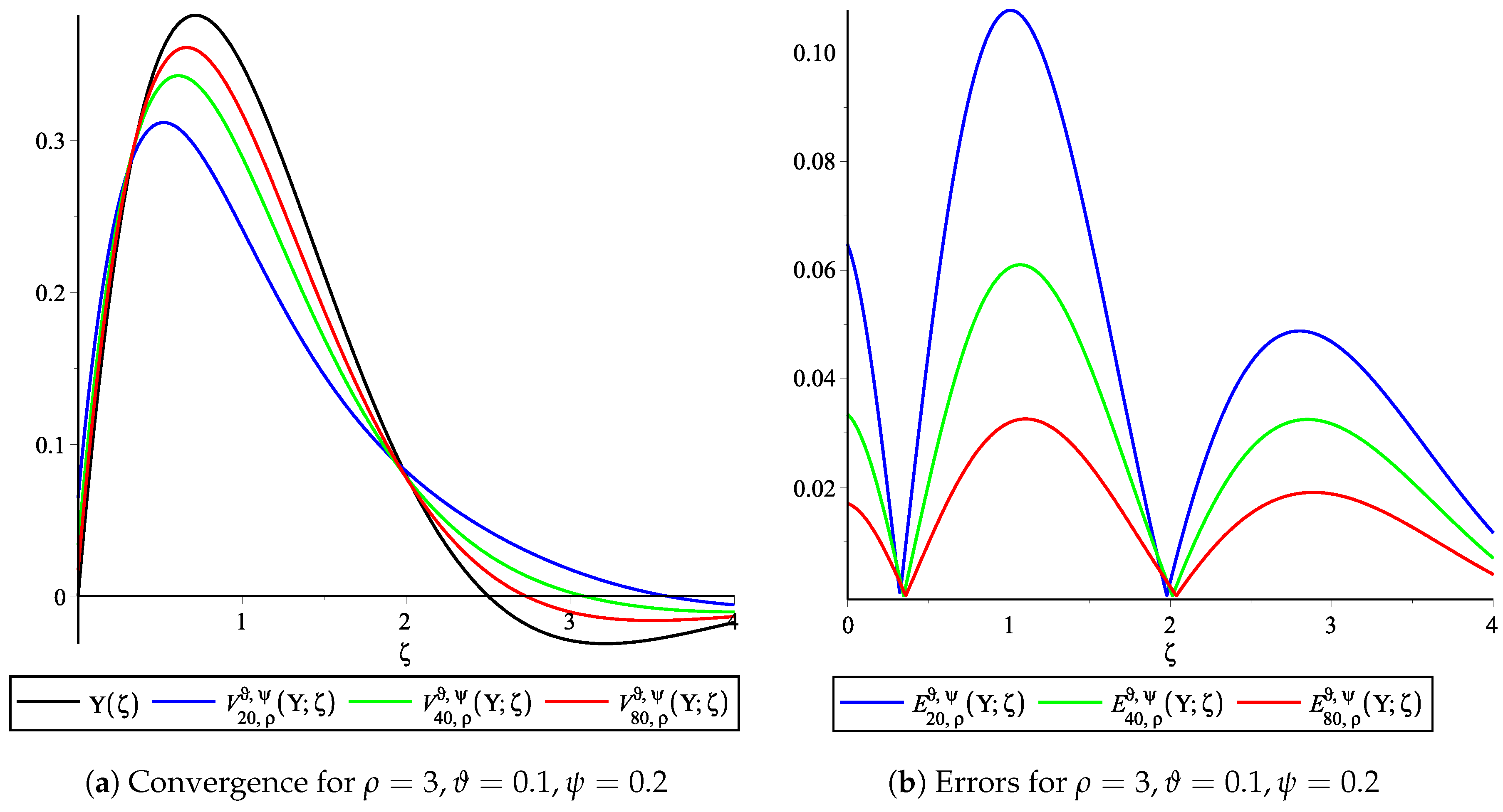
Consider the function Υ ( ζ ) = sin ( 0.4 π ζ ) e ζ . In Figure 2a, we show the convergence behavior of operators V ξ , ρ ϑ , ψ ( Υ ; ζ ) to Υ ( ζ ) for 0 ζ 4 , ρ = 3 , ϑ = 0.1 , ψ = 0.2 and ξ = 20 , 40 , 80 , respectively. Also, in Figure 2b, we define with E ξ , ρ ϑ , ψ ( Υ ; ζ ) = | V ξ , ρ ϑ , ψ ( Υ ; ζ ) Υ ( ζ ) | the absolute error of approximation of related operators to considered function. One can easily check from Figure 2 that, when ξ values increase, proposed operators V ξ , ρ ϑ , ψ ( Υ ; ζ ) provide better approximation convergence.
Example 3.
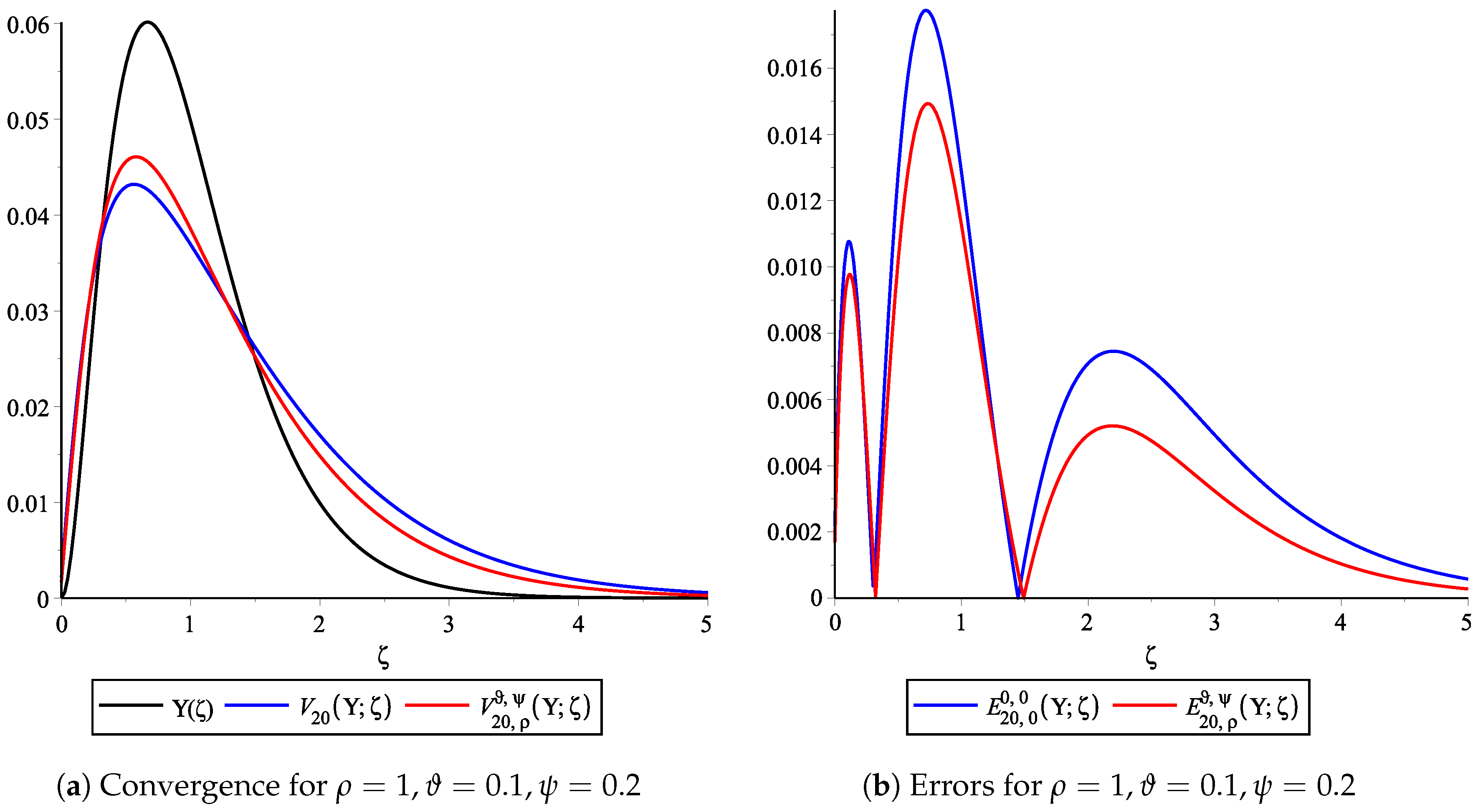
Consider the function Υ ( ζ ) = ζ 2 e 3 ζ . In Figure 3a, we compare the convergence of operators V ξ , ρ ϑ , ψ ( Υ ; ζ ) with operators V ξ ( Υ ; ζ ) for the fixed parameters 0 ζ 5 , ρ = 1 , ϑ = 0.1 , ψ = 0.2 and ξ = 20 , respectively. Also, in Figure 3b, we denote with E ξ , ρ ϑ , ψ ( Υ ; ζ ) = | V ξ , ρ ϑ , ψ ( Υ ; ζ ) Υ ( ζ ) | the absolute error of approximation of operators V ξ , ρ ϑ , ψ ( Υ ; ζ ) and V ξ ( Υ ; ζ ) to the considered function. In Figure 3, it is clearly seen that operators V ξ , ρ ϑ , ψ ( Υ ; ζ ) provide better approximation than operators V ξ ( Υ ; ζ ) .

8. Conclusions and Remarks

A novel variation of the Baskakov–Schurer–Stancu operators is presented in this paper. We derived and analyzed test functions and central moments. A Korovkin-type approximation theorem is developed based on these fundamental findings, and the weighted modulus of continuity in weighted spaces is used to analyze the rate of convergence. Additionally, functions on the Lipschitz-type class, Peetre’s K-functional and the classical modulus of continuity are used to analyze the pointwise approximation behavior. The theorem of Voronovskaja’s type is proved. Numerical examples are also provided to demonstrate the application and validity of the theoretical results. Consequently, we found that a more broad operator was developed in comparison to earlier investigations. Also, parameters ϑ , ρ , ψ used in the operators V ξ , ρ ϑ , ψ provided more flexibility in approximation.

Author Contributions

Methodology, N.F.O. and N.R.; software, M.F.; validation, M.F. and R.A.; formal analysis, M.F.; writing—original draft, N.F.O.; writing—review and editing, N.R. and R.A. All authors have read and agreed to the published version of the manuscript.

Funding

The APC was funded by the Deanship of Graduate Studies and Scientific Research at Qassim University for financial support (QU-APC-2026).

Data Availability Statement

No data were used in this manuscript.

Acknowledgments

The researchers would like to thank the Deanship of Graduate Studies and Scientific Research at Qassim University for financial support (QU-APC-2026).

Conflicts of Interest

The authors declare no conflicts of interest.

References

  1. Bernstein, S.N. Démonstration du théorème de Weierstrass fondée sur le calcul des probabilités. Comp. Comm. Soc. Mat. Charkow Ser. 1912, 13, 1–2. [Google Scholar]
  2. Schurer, F. Positive Linear Operators in Approximation Theory; Report; Mathematical Institute of the Technological University Delft: Delft, The Netherlands, 1962. [Google Scholar]
  3. Stancu, D.D. Asupra unei generalizari a polinoamelor lui Bernstein. Studia Univ. Babes-Bolyai Ser. Math.-Phys. 1969, 41, 31–45. [Google Scholar]
  4. Braha, N.L.; Mansour, T.; Özger, F.; Mursaleen, M. A new parametric formulation of Baskakov-Schurer-Szász operators with approximation properties. Adv. Stud. Euro-Tbil. Math. J. 2025, 18, 251–274. [Google Scholar] [CrossRef]
  5. Patel, P.; Rathour, L. The rate of approximation of functions in an infinite interval by positive linear operators. Georgian Math. J. 2022, 29, 575–581. [Google Scholar] [CrossRef]
  6. Mohiuddine, S.A.; Özger, F. Approximation of functions by Stancu variant of Bernstein-Kantorovich operators based on shape parameter α. Rev. R. Acad. Cienc. Exactas Fis. Nat. Ser. A Mat. 2020, 114, 70. [Google Scholar] [CrossRef]
  7. Turhan, N.; Özger, F.; Mursaleen, M. Kantorovich-Stancu type (α, λ, s)-Bernstein operators and their approximation properties. Math. Comput. Model. Dyn. Syst. 2024, 30, 228–265. [Google Scholar] [CrossRef]
  8. Yadav, J.; Mohiuddine, S.; Kajla, A.; Alotaibi, A. α-Bernstein integral type operators. Bull. Iran. Math. Soc. 2023, 49, 59. [Google Scholar] [CrossRef]
  9. Ansari, K.J.; Özger, F.; Ödemiş Özger, Z. Numerical and theoretical approximation results for Schurer-Stancu operators with shape parameter λ. Comput. Appl. Math. 2022, 41, 181. [Google Scholar] [CrossRef]
  10. Srivastava, H.M.; Ansari, K.J.; Özger, F.; Ödemis Özger, Z. A link between approximation theory and summability methods via four-dimensional infinite matrices. Mathematics 2021, 9, 1895. [Google Scholar] [CrossRef]
  11. Patel, P. On Durrmeyer variant of Mittag-Leffler operators. Dolomites Res. Notes Approx. 2025, 18, 39–46. [Google Scholar]
  12. Özger, F.; Srivastava, H.M.; Mohiuddine, S.A. Approximation of functions by a new class of generalized Bernstein-Schurer operators. Rev. R. Acad. Cienc. Exactas Fís. Nat. Ser. A Math. 2020, 114, 173. [Google Scholar] [CrossRef]
  13. Berwal, S.; Mohiuddine, S.A.; Kajla, A.; Alotaibi, A. Approximation by Riemann-Liouville type fractional α-Bernstein-Kantorovich operators. Math. Methods Appl. Sci. 2024, 47, 8275–8288. [Google Scholar] [CrossRef]
  14. Kajla, A.; Acar, T. Blending type approximation by generalized Bernstein-Durrmeyer type operators. Miskolc Math. Notes 2018, 19, 319–336. [Google Scholar] [CrossRef]
  15. Usta, F. On new modification of Bernstein operators: Theory and applications. Iran. J. Sci. Technol. Trans. Sci. 2020, 44, 1119–1124. [Google Scholar] [CrossRef]
  16. Cheng, W.T.; Mohiuddine, S.A. Construction of a new modification of Baskakov operators on (0,). Filomat 2023, 37, 139–154. [Google Scholar] [CrossRef]
  17. Baskakov, V.A. An instance of sequance of linear positive operators in the space of continuous functions. Dokl. Akad. Nauk. SSSR 1957, 113, 249–251. [Google Scholar]
  18. Gadzhiev, A.D. The convergence problem for a sequence of positive linear operators on unbounded sets, and theorems analogous to that of P.P. Korovkin. Dokl. Akad. Nauk. SSSR 1974, 218, 1001–1004. (In Russian) [Google Scholar]
  19. Gadzhiev, A.D. The convergence problem for a sequence of positive linear operators on unbounded sets, and theorems analogous to that of P.P. Korovkin. Sov. Math. Dokl. 1974, 15, 1433–1436. (In English) [Google Scholar]
  20. Gadzhiev, A.D. Theorems of the type P.P. Korovkin type theorems. Math. Zametki 1976, 5, 781–786. (In Russian) [Google Scholar]
  21. Gadzhiev, A.D. Theorems of the type P.P. Korovkin type theorems. Math. Notes 1976, 20, 996–998. (In English) [Google Scholar] [CrossRef]
  22. Ispir, N. On modified Baskakov operators on weighted spaces. Turk. J. Math. 2001, 25, 355–365. [Google Scholar]
  23. Shisha, O.; Mond, B. The degree of convergence of sequences of linear positive operators. Proc. Nat. Acad. Sci. USA 1968, 60, 1196–1200. [Google Scholar] [CrossRef] [PubMed]
  24. Peetre, J. A Theory of Interpolation of Normed Spaces; Notas de matematica 39; Instituto de Matematica Pura e Aplicada, Conselho Nacional de Pesquisas: Rio de Janeiro, Brazil, 1968. [Google Scholar]
  25. DeVore, R.A.; Lorentz, G.G. Constructive Approximation; Springer: Berlin/Heidelberg, Germany, 1993; Volume 177. [Google Scholar]
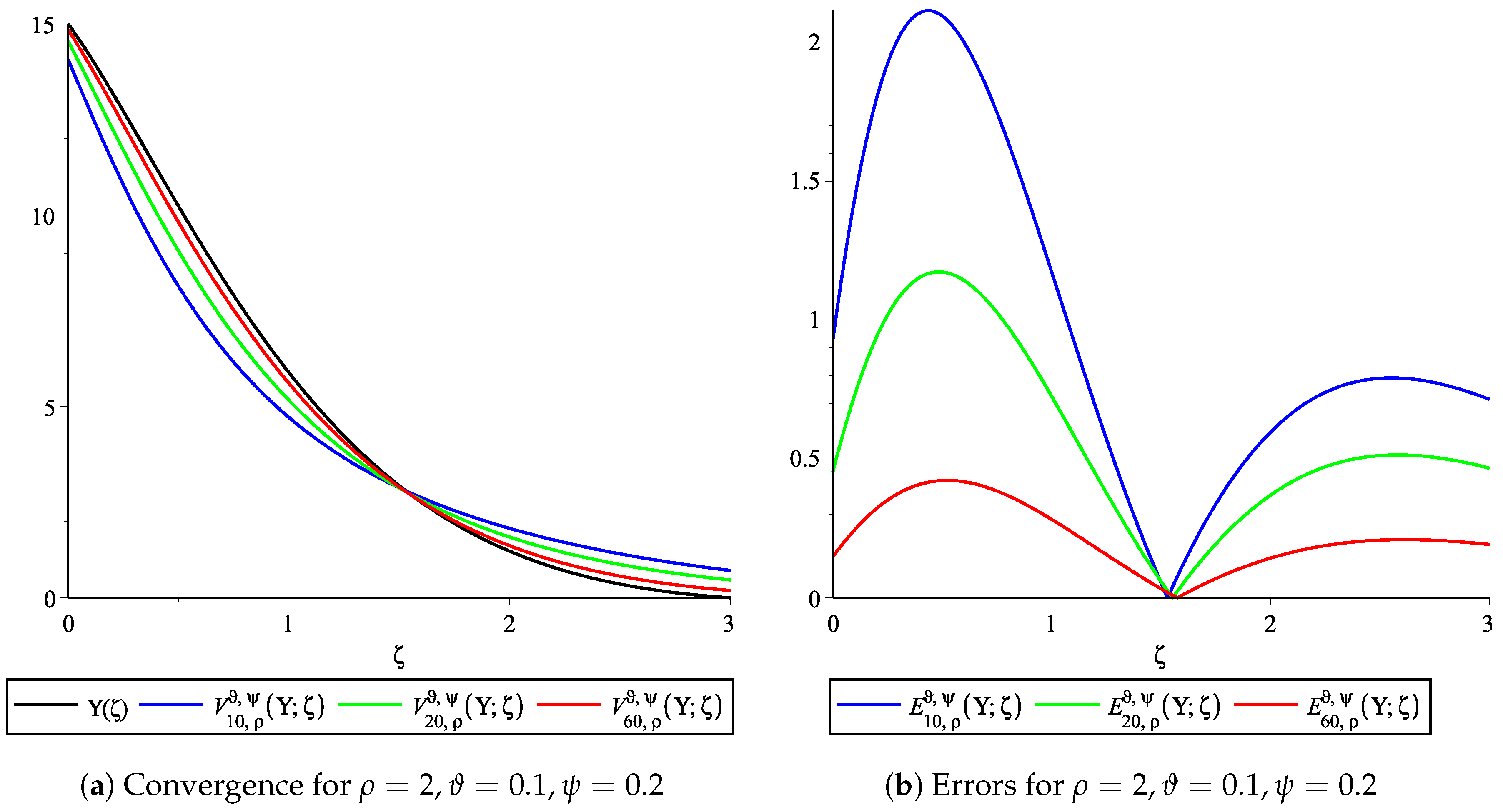
Figure 1. (a) Convergence and (b) error of approximation of operators V ξ , ρ ϑ , ψ ( Υ ; ζ ) to Υ ( ζ ) for ρ = 2 , ϑ = 0.1 , ψ = 0.2 , ξ = 10 , 20 , 60 .
Mathematics 14 00241 g001
Figure 2. (a) Convergence and (b) error of approximation of operators V ξ , ρ ϑ , ψ ( Υ ; ζ ) to Υ ( ζ ) for ρ = 3 , ϑ = 0.1 , ψ = 0.2 , ξ = 20 , 40 , 80 .
Mathematics 14 00241 g002
Figure 3. (a) Comparison of convergence and (b) error of approximation of operators V ξ , ρ ϑ , ψ ( Υ ; ζ ) with V ξ ( Υ ; ζ ) to Υ ( ζ ) for ρ = 1 , ϑ = 0.1 , ψ = 0.2 and ξ = 20 .
Mathematics 14 00241 g003
Disclaimer/Publisher’s Note: The statements, opinions and data contained in all publications are solely those of the individual author(s) and contributor(s) and not of MDPI and/or the editor(s). MDPI and/or the editor(s) disclaim responsibility for any injury to people or property resulting from any ideas, methods, instructions or products referred to in the content.