Stability and Bifurcation Structure of a Discrete-Time Chemostat Model with Nutrient Recycling

Abstract

This work aims to study the dynamic behavior of a discrete-time chemostat model involving the effect of nutrient recycling, which is a common biological phenomenon usually left out in conventional models. Based on a continuous time model involving the interrelationship between bacterial population and nutrient concentration, a new system with nutrient recycling term is obtained by introducing the process of nutrient recycling from biomass. This model is subsequently transformed to a discrete form using the forward Euler approximation scheme. Existence and stability of all possible equilibria are examined using the characteristic equation. Necessary conditions for stability and bifurcations, including transcritical and flip types, have been derived. It turns out that the considered model cannot experience Neimark–Sacker bifurcation. The results indicate that the recycling parameter plays an important role in changing stability regions and can generate complex dynamics, including oscillations and chaos. Numerical simulations are used to verify the analytical results and to show transitions between different types of system behavior. The results imply that the relationship between nutrient input, bacterial proliferation, and the recycling process has an essential influence on the dynamics and improves the comprehension of discrete ecological models.

1. Introduction

Mathematical modeling has become an essential tool for understanding the complex dynamics of biological and ecological systems. In particular, chemostat models are frequently used by microbiologists, biotechnologists, and ecologists to examine the dynamics of populations, the uptake of nutrients, and the stability of ecosystems [1,2,3]. Chemostat models have proven themselves to be an efficient tool for investigating complicated dynamics in an environment where nutrients are constantly supplied and microorganisms are removed from the environment.

Classic chemostat models usually represent the dynamics of bacterial populations based on the availability of nutrients. The interplay between biomass and nutrients can be represented using saturating functions, as the growth rate increases with the increase in nutrient availability but becomes saturated after reaching a certain level. Nonlinear interactions lead to several dynamic behaviors such as equilibrium stability, periodic behavior, and bifurcation. Understanding these dynamics is essential to determine future behaviors and devise appropriate control measures for the system.

Studies on chemostat models have significantly contributed to understanding complex biological and ecological dynamics. Pilyugin and Waltman [4] explored a chemostat model with variable yields and proved that contrary to the conventional Monod model, there was an occurrence of oscillations and subcritical Hopf bifurcation in the model, resulting in the coexistence of several limit cycles. Chemostat models with more than one limiting substrate have been considered by Mazenc and Malisoff [5], where conditions guaranteeing global asymptotic stability of the positive equilibrium points of the systems and techniques for stabilizing the controlled chemostats have been provided. Khan et al. [6] studied a chemostat model using fractional fractal derivatives and proved the existence, uniqueness, and stability of solutions, highlighting the impact of memory effects and complex media. Ben and Abdellatif [7] considered a chemostat model with inhibitory control mechanisms and showed that these controls would affect the region of stability of the system, thus giving rise to bifurcations in various forms. Sharma et al. [8] analyzed a discrete chemostat model and showed the appearance of one- and two-codimensional bifurcations, like folding, period doubling, Neimark–Sacker and resonance bifurcations, demonstrating the presence of highly complex dynamical behaviors.

In this work, we consider the following continuous-time chemostat model [9]:

$$\left\{\begin{array}{c}{\displaystyle \frac{\mathrm{d}x}{\mathrm{d}t}}={\displaystyle \frac{\alpha xy}{1+y}}-x,\hfill \\ {\displaystyle \frac{\mathrm{d}y}{\mathrm{d}t}}=-{\displaystyle \frac{xy}{1+y}}-y+\beta .\hfill \end{array}\right.$$

(1)

where $x\left(t\right)$ is the density of bacterial cells per unit volume of growth medium at time t, indicating the presence of bacteria in the chemostat. The term $y\left(t\right)$ refers to the amount of nutrients present at time t in the growth chamber, affecting the growth of bacteria. Furthermore, $\alpha$ is the natural growth rate of the bacteria, whereas $\beta$ is the supply rate of fresh nutrients to the chemostat.

Model (1) reflects the key coupling between biomass and nutrient concentration. The expression ${\displaystyle \frac{\alpha xy}{1+y}}$ models the nutrient-dependent growth via a saturating function, whereas the linear degradation rates incorporate wash-out effects. In addition, the nutrient dynamics include both uptake by the bacteria and input from an external source.

In [9], Basyouni and Khan analyzed the discrete version of system (1) which was generated by the forward Euler scheme. Their work showed that the discrete version of system (1) experiences period-doubling bifurcation. Moreover, Alsulami [10] analyzed a discretized system of Equation (1) through the use of the piecewise constant argument technique. It was found out that the discrete system experiences transcritical and period-doubling bifurcations.

Though the model (1) adequately explains several key features of the dynamics of microorganisms, it does not take into account one of the most significant factors of ecology: the regeneration of nutrients from organic matter. The actual biological world consists of organisms that do not only consume nutrients but also regenerate them through phenomena like cellular death, decay, and metabolic effluents.

To address this limitation, we extend system (1) by incorporating a nutrient recycling term, leading to the modified model:

$$\left\{\begin{array}{c}{\displaystyle \frac{\mathrm{d}x}{\mathrm{d}t}}={\displaystyle \frac{\alpha xy}{1+y}}-x,\hfill \\ {\displaystyle \frac{\mathrm{d}y}{\mathrm{d}t}}=-{\displaystyle \frac{xy}{1+y}}-y+\beta +\gamma x.\hfill \end{array}\right.$$

(2)

where the extra parameter $\gamma \ge 0$ denotes the rate of nutrient recycling from bacteria to nutrients. The expression $\gamma x$ takes into account the effects of bacteria on the recycling of nutrients via biological means such as decomposition and metabolic waste.

The incorporation of the recycling concept into the model substantially improves its dynamical properties. The interaction of consumption and production processes can be affected by recycling and thus give rise to new equilibrium configurations. In particular, the recycling process may positively influence the sustainability of bacterial communities or alter the stability criteria of equilibria.

Although continuous-time models provide valuable theoretical insights, many real-world processes evolve in discrete time due to factors such as seasonality, sampling, or numerical approximation. Moreover, continuous-time systems often do not exhibit complex behaviors such as period-doubling and chaotic dynamics due to the Poincare–Bendixson theorem [11], whereas discrete-time systems are capable of displaying such phenomena [12,13,14]. Therefore, it is of interest to study the discrete form of the model (2).

Motivated by these considerations, we discretize system (2) using the forward Euler method. This yields the following discrete system:

$$\left\{\begin{array}{c}{x}_{n+1}=x_n+h\left({\displaystyle \frac{\alpha x_n{y}_n}{1+y_n}}-x_n\right),\hfill \\ y_{n+1}=y_n+h\left(-{\displaystyle \frac{x_n{y}_n}{1+y_n}}-y_n+\beta +\gamma x_n\right),\hfill \end{array}\right.$$

(3)

where $h>0$ denotes the step size.

The primary purpose of this study is to explore the dynamical characteristics of system (3). This study highlights the existence and stability of equilibrium points and studies different types of bifurcations, such as transcritical and period-doubling bifurcations. Through detailed analysis, we derive explicit stability and bifurcation conditions, which offer an in-depth insight into the effects of model parameters on its dynamical characteristics.

The novelty of this study is based on the integration of nutrient recycling within a chemostat model and the exploration of the dynamical properties of its discrete version. The interaction between the influence of the recycling and the discrete-time nature of the system results in interesting phenomena, which have not been investigated in previous literature.

The remaining parts of the paper are structured as follows. The existence and stability of the fixed points of system (3) are examined in Section 2. Bifurcation analysis of system (3) is analyzed in Section 3, where transcritical and period-doubling bifurcations are studied via the center manifold method. Section 4 presents a comparison of continuous model (2) and discrete model (3). Section 5 discusses two approaches for controlling bifurcation and chaos in system (3). Numerical examples are provided in Section 6 to illustrate our analytical results and complexity of system (3). Finally, conclusions are drawn in Section 7 summarizing the main findings and their biological implications.

2. Topological Classification of Fixed Points

The study of the stability of the fixed points is vital for examining the dynamical behavior of the discrete chemostat model (3). Fixed points represent states where the number of bacteria and the nutrient level do not change over time. Biologically, they can be considered as extinction or persistence scenarios for the bacteria and nutrients within the framework of the model. The stability of the fixed points indicates whether the system will attain a stable state or exhibit oscillatory behavior.

2.1. Existence of Fixed Points

To find the fixed points $(x,y)$ of system (3), we solve the following system:

$$\left\{\begin{array}{c}x=x+h\left({\displaystyle \frac{\alpha xy}{1+y}}-x\right),\hfill \\ y=y+h\left(-{\displaystyle \frac{xy}{1+y}}-y+\beta +\gamma x\right),\hfill \end{array}\right.$$

(4)

The discrete system (3) admits two fixed points, namely

$$E_1=(0,\beta ),E^{*}=\left({\displaystyle \frac{\alpha (1+\beta -\alpha \beta )}{(-1+\alpha )(-1+\alpha \gamma )}},{\displaystyle \frac{1}{-1+\alpha }}\right).$$

The boundary fixed point $E_1$ always exists. It represents the extinction state of the bacterial population, where only nutrients remain in the system at a steady level set by the inflow rate $\beta$. This happens in cases where there is insufficient bacterial growth to counterbalance wash-out or negative conditions. However, the positive fixed point $E^{*}$ indicates coexistence stability where both bacteria and nutrients remain positive and stable over time. This balance exists only under the conditions $\gamma <1$, $1<\alpha <{\displaystyle \frac{1}{\gamma }}$, and $\beta >{\displaystyle \frac{1}{-1+\alpha }}$. These factors ensure that the combined effects of bacterial growth, nutrient supply, and recycling can support long-term survival.

2.2. Stability of Fixed Points

The classification of fixed points is carried out using the method described in [15,16]. The Jacobian matrix corresponding to any fixed point $(x,y)$ can be obtained by straightforward calculations as follows:

$$J(x,y)=\left[\begin{array}{cc}1+h\left(-1+{\displaystyle \frac{y\alpha }{1+y}}\right)& {\displaystyle \frac{hx\alpha }{{(1+y)}^2}}\\ h\left(-1+{\displaystyle \frac{1}{1+y}}+\gamma \right)& 1+h\left(-1-{\displaystyle \frac{x}{{(1+y)}^2}}\right)\end{array}\right].$$

Theorem 1. 

1.

If $\alpha \beta -1-\beta >0$, then $E_1$ is

(i) 

a source if $h>2$,

(ii) 

a saddle if $h<2$,

(iii) 

non-hyperbolic if $h=2$.

2.

If $\alpha \beta -1-\beta =0$, then $E_1$ is non-hyperbolic.

3.

If $\alpha \beta -1-\beta <0$, then $E_1$ is

(i) 

a sink if $h<min\left\{2,{\displaystyle \frac{2(1+\beta )}{1+\beta -\alpha \beta }}\right\}$,

(ii) 

a source if $h>max\left\{2,{\displaystyle \frac{2(1+\beta )}{1+\beta -\alpha \beta }}\right\}$,

(iii) 

a saddle if $min\left\{2,{\displaystyle \frac{2(1+\beta )}{1+\beta -\alpha \beta }}\right\}<h<max\left\{2,{\displaystyle \frac{2(1+\beta )}{1+\beta -\alpha \beta }}\right\}$,

(iv) 

non-hyperbolic if either of the subsequent conditions is satisfied:

(a) 

$h=2$,

(b) 

$h={\displaystyle \frac{2(1+\beta )}{1+\beta -\alpha \beta }}$.

Proof. 

We obtain

$$J\left(E_1\right)=\left[\begin{array}{cc}1+h\left(-1+{\displaystyle \frac{\alpha \beta }{1+\beta }}\right)& 0\\ h\left(-{\displaystyle \frac{\beta }{1+\beta }}+\gamma \right)& 1-h\end{array}\right].$$

The eigenvalues of $J\left(E_1\right)$ are ${\xi }_1=1+h\left(-1+{\displaystyle \frac{\alpha \beta }{1+\beta }}\right)$ and ${\xi }_2=1-h$. We check that

$$\left|{\xi }_2\right|\left\{\begin{array}{cc}<1,\hfill & \mathrm{if}h<2,\hfill \\ =1,\hfill & \mathrm{if}h=2,\hfill \\ >1,\hfill & \mathrm{if}h>2.\hfill \end{array}\right.$$

(5)

Moreover, it is clear that $\alpha \beta -1-\beta =0$ implies ${\xi }_1=1$. Setting $\alpha \beta -1-\beta >0$ implies ${\xi }_1>1$. Additionally, $\alpha \beta -1-\beta <0$ yields the following:

$$\left|{\xi }_1\right|\left\{\begin{array}{cc}<1,\hfill & \mathrm{if}h<{\displaystyle \frac{2(1+\beta )}{1+\beta -\alpha \beta }},\hfill \\ =1,\hfill & \mathrm{if}h={\displaystyle \frac{2(1+\beta )}{1+\beta -\alpha \beta }},\hfill \\ >1,\hfill & \mathrm{if}h>{\displaystyle \frac{2(1+\beta )}{1+\beta -\alpha \beta }}.\hfill \end{array}\right.$$

(6)

□

Next, we compute the Jacobian matrix at the positive fixed point $E^{*}$ as

$$J\left(E^{*}\right)=\left[\begin{array}{cc}1& -{\displaystyle \frac{h(-1+\alpha )(-1+(-1+\alpha \left)\beta \right)}{-1+\alpha \gamma }}\\ h\left(-{\displaystyle \frac{1}{\alpha }}+\gamma \right)& 1+{\displaystyle \frac{h\left(1+{(-1+\alpha )}^2\beta -{\alpha }^2\gamma \right)}{\alpha (-1+\alpha \gamma )}}\end{array}\right].$$

(7)

The characteristic polynomial corresponding to $J\left(E^{*}\right)$ is given by

$$\Lambda \left(\xi \right)={\xi }^2+K_1\xi +K_0,$$

where

$$\begin{array}{cc}\hfill K_1& =-2-{\displaystyle \frac{h\left(1+{(-1+\alpha )}^2\beta -{\alpha }^2\gamma \right)}{\alpha (-1+\alpha \gamma )}},\hfill \\ \hfill K_0& =1+{\displaystyle \frac{h^2(-1+\alpha )(-1+(-1+\alpha )\beta )}{\alpha }}+{\displaystyle \frac{h\left(1+{(-1+\alpha )}^2\beta -{\alpha }^2\gamma \right)}{\alpha (-1+\alpha \gamma )}}.\hfill \end{array}$$

A straightforward computation yields that

$$\begin{array}{cc}\hfill \Lambda \left(0\right)& =1+{\displaystyle \frac{h^2(-1+\alpha )(-1+(-1+\alpha )\beta )}{\alpha }}+{\displaystyle \frac{h\left(1+{(-1+\alpha )}^2\beta -{\alpha }^2\gamma \right)}{\alpha (-1+\alpha \gamma )}},\hfill \\ \hfill \Lambda (-1)& =4+{\displaystyle \frac{h\left(h(-1+\alpha )(-1+(-1+\alpha )\beta )+\frac{2\left(1+{(-1+\alpha )}^2\beta -{\alpha }^2\gamma \right)}{-1+\alpha \gamma }\right)}{\alpha }},\hfill \\ \hfill \Lambda \left(1\right)& ={\displaystyle \frac{h^2(-1+\alpha )(-1+(-1+\alpha )\beta )}{\alpha }}.\hfill \end{array}$$

Clearly, $\Lambda \left(1\right)>0$. We can rewrite $\Lambda \left(0\right)$ and $\Lambda (-1)$ as follows:

$$\begin{array}{cc}\hfill \Lambda \left(0\right)& ={\displaystyle \frac{{(\alpha -1)}^2\beta h(\alpha \gamma h-h+1)}{\alpha (\alpha \gamma -1)}}-{\displaystyle \frac{\alpha +\alpha \gamma \left(h\right(\alpha +(\alpha -1)h)-\alpha )+h(-\alpha h+h-1)}{\alpha (\alpha \gamma -1)}},\hfill \\ \hfill \Lambda (-1)& =4-{\displaystyle \frac{(\alpha -1)h^2}{\alpha }}-{\displaystyle \frac{2h\left({\alpha }^2\gamma -1\right)}{\alpha (\alpha \gamma -1)}}+{\displaystyle \frac{{(\alpha -1)}^2\beta h(\alpha \gamma h-h+2)}{\alpha (\alpha \gamma -1)}}.\hfill \end{array}$$

Theorem 2. 

The positive fixed point $E^{*}$ is

1.

a sink if $4-{\displaystyle \frac{(\alpha -1)h^2}{\alpha }}-{\displaystyle \frac{2h\left({\alpha }^2\gamma -1\right)}{\alpha (\alpha \gamma -1)}}+{\displaystyle \frac{{(\alpha -1)}^2\beta h(\alpha \gamma h-h+2)}{\alpha (\alpha \gamma -1)}}>0,1-h+h\alpha \gamma <0$ and $\beta <{\displaystyle \frac{{\alpha }^2\gamma +(\alpha -1)h(\alpha \gamma -1)-1}{{(\alpha -1)}^2(h(\alpha \gamma -1)+1)}}$,

2.

a source if $4-{\displaystyle \frac{(\alpha -1)h^2}{\alpha }}-{\displaystyle \frac{2h\left({\alpha }^2\gamma -1\right)}{\alpha (\alpha \gamma -1)}}+{\displaystyle \frac{{(\alpha -1)}^2\beta h(\alpha \gamma h-h+2)}{\alpha (\alpha \gamma -1)}}>0,1-h+h\alpha \gamma <0$ and $\beta >{\displaystyle \frac{{\alpha }^2\gamma +(\alpha -1)h(\alpha \gamma -1)-1}{{(\alpha -1)}^2(h(\alpha \gamma -1)+1)}}$,

3.

a saddle if $4-{\displaystyle \frac{(\alpha -1)h^2}{\alpha }}-{\displaystyle \frac{2h\left({\alpha }^2\gamma -1\right)}{\alpha (\alpha \gamma -1)}}+{\displaystyle \frac{{(\alpha -1)}^2\beta h(\alpha \gamma h-h+2)}{\alpha (\alpha \gamma -1)}}<0$,

4.

non-hyperbolic and the system (3) experiences period-doubling bifurcation at $E^{*}$ if

$${\displaystyle \frac{h\left(1+{(-1+\alpha )}^2\beta -{\alpha }^2\gamma \right)}{\alpha (1-\alpha \gamma )}}\ne 2,4,\mathit{and}4-{\displaystyle \frac{(\alpha -1)h^2}{\alpha }}-{\displaystyle \frac{2h\left({\alpha }^2\gamma -1\right)}{\alpha (\alpha \gamma -1)}}+{\displaystyle \frac{{(\alpha -1)}^2\beta h(\alpha \gamma h-h+2)}{\alpha (\alpha \gamma -1)}}=0.$$

Next, we show that system (3) does not undergo a Neimark–Sacker bifurcation at the positive fixed point $E^{*}$. For a Neimark–Sacker bifurcation to occur, the conditions $\Lambda \left(0\right)=1$ and $K_1^2-4K_0<0$ must be satisfied. These are equivalent to $\Lambda \left(0\right)=K_0=1$ and $-2<K_1<2$. The equation $\Lambda \left(0\right)=1$ can be written as follows:

$$\beta -{\displaystyle \frac{1}{\alpha -1}}={\displaystyle \frac{\alpha (\alpha \gamma -1)}{{(\alpha -1)}^2(1-h+h\alpha \gamma )}}.$$

(8)

Using the existence conditions for $E^{*}$

$$\gamma <1,1<\alpha <{\displaystyle \frac{1}{\gamma }},\beta >{\displaystyle \frac{1}{\alpha -1}},$$

together with (8) yields $1-h+h\alpha \gamma <0$. Next, substituting the value of $\beta$ from (8) into

$$K_1=-2-{\displaystyle \frac{h\left(1+{(-1+\alpha )}^2\beta -{\alpha }^2\gamma \right)}{\alpha (-1+\alpha \gamma )}},$$

we obtain the reduced form

$$K_1=-2+h-{\displaystyle \frac{h}{1-h+h\alpha \gamma }}.$$

(9)

We can write

$$\begin{array}{cc}\hfill K_1& =-2+h-{\displaystyle \frac{h}{1-h+h\alpha \gamma }}\hfill \\ \hfill & >-2+h-{\displaystyle \frac{h}{1-h}}.(\mathrm{because}1-h+h\alpha \gamma >1-h)\hfill \end{array}$$

Moreover,

$$\begin{array}{cc}\hfill & 1-h+h\alpha \gamma <0\hfill \\ \hfill & h(1-\alpha \gamma )>1\hfill \\ \hfill & h>{\displaystyle \frac{1}{1-\alpha \gamma }}>1.(\mathrm{because}\alpha \gamma >0\Rightarrow 1-\alpha \gamma <1)\hfill \end{array}$$

Since $h>1$, therefore we have

$$\begin{array}{c}\hfill h-{\displaystyle \frac{h}{1-h}}-4={\displaystyle \frac{{(h-2)}^2}{h-1}}\ge 0\Rightarrow h-{\displaystyle \frac{h}{1-h}}\ge 4.\end{array}$$

As a result, we have

$$\begin{array}{c}\hfill K_1>-2+h-{\displaystyle \frac{h}{1-h}}\ge -2+4=2\end{array}$$

Thus, $K_1>2$, and consequently the condition $-2<K_1<2$ cannot be satisfied. Hence, the system (3) does not experience a Neimark–Sacker bifurcation at $E^{*}$.

The above exclusion also admits a direct spectral-geometric interpretation. Let ${\xi }_1$ and ${\xi }_2$ denote the eigenvalues of $J\left(E^{*}\right)$. From the characteristic polynomial $\Lambda \left(\xi \right)={\xi }^2+K_1\xi +K_0,$ one has

$${\xi }_1+{\xi }_2=-K_1,{\xi }_1{\xi }_2=K_0.$$

At the Neimark–Sacker condition $K_0=1$, the above analysis gives $K_1>2$. Hence,

$$K_1^2-4K_0=K_1^2-4>0,$$

so the two eigenvalues are real. Furthermore, ${\xi }_1{\xi }_2=1>0$ implies that the real eigenvalues have the same sign, while ${\xi }_1+{\xi }_2=-K_1<-2$ implies that both are negative. Since ${\xi }_1{\xi }_2=1$, they are reciprocal, with one eigenvalue lying in $(-\infty ,-1)$ and the other in $(-1,0)$. Thus, the spectrum lies on the negative real axis rather than forming a complex-conjugate pair on the unit circle.

This indicates that the system (3) does not exhibit Neimark–Sacker bifurcation leading quasiperiodic oscillations around the coexistence equilibrium $E^{*}$. From a biological perspective, this implies that the interaction between bacterial growth, nutrient consumption, and recycling does not generate sustained cyclic behavior driven by Neimark–Sacker bifurcation. Instead, the system dynamics are primarily governed by transitions involving stability, period-doubling, and possible chaotic behavior.

3. Bifurcation Analysis

This section discusses the dynamical properties of the discrete chemostat model (3) through a comprehensive bifurcation analysis, especially for transcritical and period-doubling bifurcations. Bifurcations represent the dynamic properties of a system as the parameters of the system change, and they are essential in studying various biological phenomena like extinction, coexistence, and oscillation within a certain biological system. The application of bifurcation theory is necessary for a deeper understanding of the interactions between bacteria growth, nutrient input, and recycling in our model. For more details on bifurcations, see [17,18,19].

3.1. Transcritical Bifurcation at $E_1$

The transcritical bifurcation at $E_1$ is studied using condition $\left(4\right)$ as given in Theorem 1. The critical condition $\alpha \beta -1-\beta =0$ gives ${\beta }_1={\displaystyle \frac{1}{\alpha -1}},\alpha >1$, at which $E_1$ becomes non-hyperbolic with a unit eigenvalue. To investigate the local dynamics near this critical value, the bifurcation parameter is perturbed as $\beta ={\beta }_1+ϵ$. Accordingly, system (3) becomes

$$\left\{\begin{array}{c}{x}_{n+1}=x_n+h\left({\displaystyle \frac{\alpha x_n{y}_n}{1+y_n}}-x_n\right),\hfill \\ y_{n+1}=y_n+h\left(-{\displaystyle \frac{x_n{y}_n}{1+y_n}}-y_n+({\beta }_1+ϵ)+\gamma x_n\right).\hfill \end{array}\right.$$

(10)

To perform the local center-manifold analysis, we translate $E_1$ to $(0,0)$ using the substitution ${\sigma }_n=x_n,$${\tau }_n=y_n-({\beta }_1+ϵ)$. As a result, system (10) can be expressed as:

$$\left[\begin{array}{c}{\sigma }_{n+1}\\ {\tau }_{n+1}\end{array}\right]=\left[\begin{array}{cc}1& 0\\ h(-{\displaystyle \frac{1}{\alpha }}+\gamma )& 1-h\end{array}\right]\left[\begin{array}{c}{\sigma }_n\\ {\tau }_n\end{array}\right]+\left[\begin{array}{c}{\mathbb{F}}_1({\sigma }_n,{\tau }_n,ϵ)\\ {\mathbb{F}}_2({\sigma }_n,{\tau }_n,ϵ)\end{array}\right],$$

(11)

where

$$\begin{array}{cc}\hfill {\mathbb{F}}_1({\sigma }_n,{\tau }_n,ϵ)& =a_1{\sigma }_n{\tau }_n+a_2{\sigma }_nϵ+a_3{\sigma }_n{\tau }_n^2+a_4{\sigma }_n{ϵ}^2+a_5{\sigma }_n{\tau }_nϵ+O\left(4\right),\hfill \\ \hfill {\mathbb{F}}_2({\sigma }_n,{\tau }_n,ϵ)& =b_1{\sigma }_n{\tau }_n+b_2{\sigma }_nϵ+b_3{\sigma }_n{\tau }_n^2+b_4{\sigma }_n{ϵ}^2+b_5{\sigma }_n{\tau }_nϵ+O\left(4\right),\hfill \end{array}$$

$$\begin{array}{cc}\hfill a_1& ={\displaystyle \frac{h{(-1+\alpha )}^2}{\alpha }},a_2={\displaystyle \frac{h{(-1+\alpha )}^2}{\alpha }},a_3=-{\displaystyle \frac{h{(-1+\alpha )}^3}{{\alpha }^2}},a_4=-{\displaystyle \frac{h{(-1+\alpha )}^3}{{\alpha }^2}},a_5=-{\displaystyle \frac{2h{(-1+\alpha )}^3}{{\alpha }^2}},\hfill \end{array}$$

$$\begin{array}{cc}\hfill b_1& =-{\displaystyle \frac{h{(-1+\alpha )}^2}{{\alpha }^2}},b_2=-{\displaystyle \frac{h{(-1+\alpha )}^2}{{\alpha }^2}},b_3={\displaystyle \frac{h{(-1+\alpha )}^3}{{\alpha }^3}},b_4={\displaystyle \frac{h{(-1+\alpha )}^3}{{\alpha }^3}},b_5={\displaystyle \frac{2h{(-1+\alpha )}^3}{{\alpha }^3}}.\hfill \end{array}$$

At $ϵ=0$, the linear part of system (11) has eigenvalues 1 and $1-h$. The eigenvalue 1 is the critical eigenvalue associated with the transcritical bifurcation. To separate the corresponding critical eigendirection from the noncritical one, a transformation matrix is constructed using the eigenvectors associated with these two eigenvalues. Accordingly, system (11) is diagonalized by the following transformation:

$$\left[\begin{array}{c}{\sigma }_n\\ {\tau }_n\end{array}\right]=\left[\begin{array}{cc}{\displaystyle \frac{\alpha }{-1+\alpha \gamma }}& 0\\ 1& 1\end{array}\right]\left[\begin{array}{c}{\mu }_n\\ {\lambda }_n\end{array}\right].$$

(12)

Under the transformation (12), (11) becomes

$$\left[\begin{array}{c}{\mu }_{n+1}\\ {\lambda }_{n+1}\end{array}\right]=\left[\begin{array}{cc}1& 0\\ 0& 1-h\end{array}\right]\left[\begin{array}{c}{\mu }_n\\ {\lambda }_n\end{array}\right]+\left[\begin{array}{c}{\mathbb{G}}_1({\mu }_n,{\lambda }_n,ϵ)\\ {\mathbb{G}}_2({\mu }_n,{\lambda }_n,ϵ)\end{array}\right],$$

(13)

where

$$\begin{array}{cc}\hfill {\mathbb{G}}_1({\mu }_n,{\lambda }_n,ϵ)& =c_1{\mu }_n^2+c_2{\mu }_n{\lambda }_n+c_3{\mu }_nϵ+c_4{\mu }_n^3+c_5{\mu }_n^2{\lambda }_n+c_6{\mu }_n^2ϵ+c_7{\mu }_n{\lambda }_n^2+c_8{\mu }_n{ϵ}^2+c_9{\mu }_n{\lambda }_nϵ+O\left(4\right),\hfill \\ \hfill {\mathbb{G}}_2({\mu }_n,{\lambda }_n,ϵ)& =d_1{\mu }_n^2+d_2{\mu }_n{\lambda }_n+d_3{\mu }_nϵ+d_4{\mu }_n^3+d_5{\mu }_n^2{\lambda }_n+d_6{\mu }_n^2ϵ+d_7{\mu }_n{\lambda }_n^2+d_8{\mu }_n{ϵ}^2+d_9{\mu }_n{\lambda }_nϵ+O\left(4\right),\hfill \end{array}$$

$$\begin{array}{cc}\hfill c_1& ={\displaystyle \frac{h{(-1+\alpha )}^2}{\alpha }},c_2={\displaystyle \frac{h{(-1+\alpha )}^2}{\alpha }},c_3={\displaystyle \frac{h{(-1+\alpha )}^2}{\alpha }},c_4=-{\displaystyle \frac{h{(-1+\alpha )}^3}{{\alpha }^2}},c_5=-{\displaystyle \frac{2h{(-1+\alpha )}^3}{{\alpha }^2}},\hfill \end{array}$$

$$\begin{array}{cc}\hfill c_6& =-{\displaystyle \frac{2h{(-1+\alpha )}^3}{{\alpha }^2}},c_7=-{\displaystyle \frac{h{(-1+\alpha )}^3}{{\alpha }^2}},c_8=-{\displaystyle \frac{h{(-1+\alpha )}^3}{{\alpha }^2}},c_9=-{\displaystyle \frac{2h{(-1+\alpha )}^3}{{\alpha }^2}},\hfill \end{array}$$

$$\begin{array}{cc}\hfill d_1& =-{\displaystyle \frac{h{(-1+\alpha )}^2\gamma }{-1+\alpha \gamma }},d_2=-{\displaystyle \frac{h{(-1+\alpha )}^2\gamma }{-1+\alpha \gamma }},d_3=-{\displaystyle \frac{h{(-1+\alpha )}^2\gamma }{-1+\alpha \gamma }},d_4={\displaystyle \frac{h{(-1+\alpha )}^3\gamma }{\alpha (-1+\alpha \gamma )}},d_5={\displaystyle \frac{2h{(-1+\alpha )}^3\gamma }{\alpha (-1+\alpha \gamma )}},\hfill \end{array}$$

$$\begin{array}{cc}\hfill d_6& ={\displaystyle \frac{2h{(-1+\alpha )}^3\gamma }{\alpha (-1+\alpha \gamma )}},d_7={\displaystyle \frac{h{(-1+\alpha )}^3\gamma }{\alpha (-1+\alpha \gamma )}},d_8={\displaystyle \frac{h{(-1+\alpha )}^3\gamma }{\alpha (-1+\alpha \gamma )}},d_9={\displaystyle \frac{2h{(-1+\alpha )}^3\gamma }{\alpha (-1+\alpha \gamma )}}.\hfill \end{array}$$

Since the critical eigenvalue is 1, the local dynamics responsible for the transcritical bifurcation can be reduced to the corresponding one-dimensional center manifold. Let $Q^C$ denote the center manifold of (13) at the origin for $ϵ$ near zero, represented locally as

$$Q^C=\left\{({\mu }_n,{\lambda }_n,ϵ)\in {\mathbb{R}}_{+}^3|{\lambda }_n=H({\mu }_n,ϵ)=p_1{\mu }_n^2+p_2{\mu }_nϵ+p_3{ϵ}^2+O\left(3\right)\right\}.$$

Substituting the center manifold expansion into (13), we obtain

$$\begin{array}{cc}\hfill {\lambda }_{n+1}& =H({\mu }_{n+1},ϵ)=H({\mu }_n+{\mathbb{G}}_1({\mu }_n,H({\mu }_n,ϵ),ϵ),ϵ),\hfill \end{array}$$

(14)

$$\begin{array}{cc}\hfill {\lambda }_{n+1}& =(1-h){\lambda }_n+{\mathbb{G}}_2({\mu }_n,{\lambda }_n,ϵ)=(1-h)H({\mu }_n,ϵ)+{\mathbb{G}}_2({\mu }_n,H({\mu }_n,ϵ),ϵ).\hfill \end{array}$$

(15)

Equating the right-hand sides of (14) and (15) and comparing the coefficients of ${\mu }_n^2$, ${\mu }_nϵ$, and ${ϵ}^2$ yields

$$\begin{array}{cc}\hfill p_1& ={\displaystyle \frac{{(-1+\alpha )}^2\gamma }{1-\alpha \gamma }},p_2={\displaystyle \frac{{(-1+\alpha )}^2\gamma }{1-\alpha \gamma }},p_3=0.\hfill \end{array}$$

Consequently, the restriction of (13) to $Q^C$ is

$$\begin{array}{cc}\hfill \mathrm{\Phi }({\mu }_n,ϵ):={\mu }_{n+1}& ={\mu }_n+{\displaystyle \frac{h{(-1+\alpha )}^2}{\alpha }}{\mu }_n^2+{\displaystyle \frac{h{(-1+\alpha )}^2}{\alpha }}{\mu }_nϵ-{\displaystyle \frac{h{(-1+\alpha )}^3(-1+{\alpha }^2\gamma )}{{\alpha }^2(-1+\alpha \gamma )}}{\mu }_n^3\hfill \\ \hfill & -{\displaystyle \frac{h{(-1+\alpha )}^3(-2+\alpha (1+\alpha )\gamma )}{{\alpha }^2(-1+\alpha \gamma )}}{\mu }_n^2ϵ-{\displaystyle \frac{h{(-1+\alpha )}^3}{{\alpha }^2}}{\mu }_n{ϵ}^2+O\left(4\right).\hfill \end{array}$$

(16)

To verify the nondegeneracy conditions for the transcritical bifurcation, the required derivatives of the reduced map $\mathrm{\Phi }({\mu }_n,ϵ)$ at $({\mu }_n,ϵ)=(0,0)$ are evaluated as

$$\begin{array}{cc}\hfill & \mathrm{\Phi }(0,0)=0,{\mathrm{\Phi }}_{{\mu }_n}(0,0)=1,{\mathrm{\Phi }}_{ϵ}(0,0)=0,\hfill \\ \hfill & {\mathrm{\Phi }}_{{\mu }_n{\mu }_n}(0,0)={\displaystyle \frac{2h{(-1+\alpha )}^2}{\alpha }}\ne 0,{\mathrm{\Phi }}_{{\mu }_nϵ}(0,0)={\displaystyle \frac{h{(-1+\alpha )}^2}{\alpha }}\ne 0.\hfill \end{array}$$

Thus, the reduced map has a unit multiplier at the critical point, while the nonzero values of ${\mathrm{\Phi }}_{{\mu }_n{\mu }_n}$ and ${\mathrm{\Phi }}_{{\mu }_nϵ}$ verify the required nondegeneracy conditions for the transcritical bifurcation.

Theorem 3. 

If condition $\left(4\right)$ in Theorem 1 is fulfilled, then (3) goes through transcritical bifurcation at $E_1$ if β varies within a close neighborhood of ${\beta }_1={\displaystyle \frac{1}{\alpha -1}}$.

Transcritical bifurcation at $E_1$ is the switch of stability between the boundary equilibrium point $E_1$ and the positive equilibrium point $E^{*}$. In terms of biology, it implies that there is a critical level where the bacteria change from becoming extinct to surviving. The switching from extinction to coexistence occurs when the parameter $\beta$ surpasses the critical value of ${\beta }_1={\displaystyle \frac{1}{\alpha -1}}$. This reveals that the provision of nutrients plays a crucial role in supporting the growth of the bacteria.

3.2. Period-Doubling Bifurcation at $E_1$

The period-doubling bifurcation at $E_1$ is investigated using condition $(3-iv-b)$ of Theorem 1. After adding a slight perturbation $ϵ$ to h around $h_1={\displaystyle \frac{2(1+\beta )}{1+\beta -\alpha \beta }}$, system (3) becomes

$$\left\{\begin{array}{c}{x}_{n+1}=x_n+(h_1+ϵ)\left({\displaystyle \frac{\alpha x_n{y}_n}{1+y_n}}-x_n\right),\hfill \\ y_{n+1}=y_n+(h_1+ϵ)\left(-{\displaystyle \frac{x_n{y}_n}{1+y_n}}-y_n+\beta +\gamma x_n\right).\hfill \end{array}\right.$$

(17)

To perform the local center-manifold analysis, the equilibrium $E_1$ is translated to the origin by setting ${\sigma }_n=x_n$, ${\tau }_n=y_n-\beta$. Consequently, (17) takes the form

$$\left[\begin{array}{c}{\sigma }_{n+1}\\ {\tau }_{n+1}\end{array}\right]=\left[\begin{array}{cc}-1& 0\\ -{\displaystyle \frac{2\left(\beta \right(-1+\gamma )+\gamma )}{-1+(-1+\alpha )\beta }}& {\displaystyle \frac{1+\beta +\alpha \beta }{-1+(-1+\alpha )\beta }}\end{array}\right]\left[\begin{array}{c}{\sigma }_n\\ {\tau }_n\end{array}\right]+\left[\begin{array}{c}{\mathbb{F}}_1({\sigma }_n,{\tau }_n,ϵ)\\ {\mathbb{F}}_2({\sigma }_n,{\tau }_n,ϵ)\end{array}\right],$$

(18)

where

$$\begin{array}{cc}\hfill {\mathbb{F}}_1({\sigma }_n,{\tau }_n,ϵ)& =a_1{\sigma }_n{\tau }_n+a_2{\sigma }_nϵ+a_3{\sigma }_n{\tau }_n^2+a_4{\sigma }_n{\tau }_nϵ+O\left(4\right),\hfill \\ \hfill {\mathbb{F}}_2({\sigma }_n,{\tau }_n,ϵ)& =b_1{\sigma }_n{\tau }_n+b_2{\sigma }_nϵ+b_3{\tau }_nϵ+b_4{\sigma }_n{\tau }_n^2+b_5{\sigma }_n{\tau }_nϵ+O\left(4\right),\hfill \end{array}$$

$$\begin{array}{cc}\hfill a_1& =-{\displaystyle \frac{2\alpha }{(1+\beta )(-1+(-1+\alpha \left)\beta \right)}},a_2=-1+{\displaystyle \frac{\alpha \beta }{1+\beta }},a_3={\displaystyle \frac{2\alpha }{{(1+\beta )}^2(-1+(-1+\alpha )\beta )}},a_4={\displaystyle \frac{\alpha }{{(1+\beta )}^2}},\hfill \end{array}$$

$$\begin{array}{cc}\hfill b_1& ={\displaystyle \frac{2}{(1+\beta )(-1+(-1+\alpha \left)\beta \right)}},b_2=-{\displaystyle \frac{\beta }{1+\beta }}+\gamma ,b_3=-1,b_4=-{\displaystyle \frac{2}{{(1+\beta )}^2(-1+(-1+\alpha )\beta )}},b_5=-{\displaystyle \frac{1}{{(1+\beta )}^2}}.\hfill \end{array}$$

At $ϵ=0$, the linear part of (18) has eigenvalues ${\xi }_1=-1$ and ${\xi }_2={\displaystyle \frac{1+\beta +\alpha \beta }{-1+(-1+\alpha )\beta }}$. The eigenvalue $-1$ is the critical eigenvalue associated with the period-doubling bifurcation. To separate the corresponding critical eigendirection from the noncritical one, a transformation matrix is constructed using the eigenvectors associated with these two eigenvalues. Accordingly, system (18) is diagonalized by the following transformation:

$$\left[\begin{array}{c}{\sigma }_n\\ {\tau }_n\end{array}\right]=\left[\begin{array}{cc}{\displaystyle \frac{\alpha \beta }{-\beta +\gamma +\beta \gamma }}& 0\\ 1& 1\end{array}\right]\left[\begin{array}{c}{\mu }_n\\ {\lambda }_n\end{array}\right].$$

(19)

Applying the transformation (19), system (18) is rewritten as follows:

$$\left[\begin{array}{c}{\mu }_{n+1}\\ {\lambda }_{n+1}\end{array}\right]=\left[\begin{array}{cc}-1& 0\\ 0& {\displaystyle \frac{1+\beta +\alpha \beta }{-1+(-1+\alpha )\beta }}\end{array}\right]\left[\begin{array}{c}{\mu }_n\\ {\lambda }_n\end{array}\right]+\left[\begin{array}{c}{\mathbb{G}}_1({\mu }_n,{\lambda }_n,ϵ)\\ {\mathbb{G}}_2({\mu }_n,{\lambda }_n,ϵ)\end{array}\right],$$

(20)

where

$$\begin{array}{cc}\hfill {\mathbb{G}}_1({\mu }_n,{\lambda }_n,ϵ)& =c_1{\mu }_n^2+c_2{\mu }_n{\lambda }_n+c_3{\mu }_nϵ+c_4{\mu }_n^3+c_5{\mu }_n^2{\lambda }_n+c_6{\mu }_n^2ϵ+c_7{\mu }_n{\lambda }_n^2+c_8{\mu }_n{\lambda }_nϵ+O\left(4\right),\hfill \\ \hfill {\mathbb{G}}_2({\mu }_n,{\lambda }_n,ϵ)& =d_1{\mu }_n^2+d_2{\mu }_n{\lambda }_n+d_3{\lambda }_nϵ+d_4{\mu }_n^3+d_5{\mu }_n^2{\lambda }_n+d_6{\mu }_n^2ϵ+d_7{\mu }_n{\lambda }_n^2+d_8{\mu }_n{\lambda }_nϵ+O\left(4\right),\hfill \end{array}$$

$$\begin{array}{cc}\hfill c_1& =-{\displaystyle \frac{2\alpha }{(1+\beta )(-1+(-1+\alpha \left)\beta \right)}},c_2=-{\displaystyle \frac{2\alpha }{(1+\beta )(-1+(-1+\alpha \left)\beta \right)}},c_3=-1+{\displaystyle \frac{\alpha \beta }{1+\beta }},\hfill \end{array}$$

$$\begin{array}{cc}\hfill c_4& ={\displaystyle \frac{2\alpha }{{(1+\beta )}^2(-1+(-1+\alpha )\beta )}},c_5={\displaystyle \frac{4\alpha }{{(1+\beta )}^2(-1+(-1+\alpha )\beta )}},c_6={\displaystyle \frac{\alpha }{{(1+\beta )}^2}},\hfill \end{array}$$

$$\begin{array}{cc}\hfill c_7& ={\displaystyle \frac{2\alpha }{{(1+\beta )}^2(-1+(-1+\alpha )\beta )}},c_8={\displaystyle \frac{\alpha }{{(1+\beta )}^2}},d_1={\displaystyle \frac{2\alpha \gamma }{(-1+(-1+\alpha \left)\beta \right)\left(\beta \right(-1+\gamma )+\gamma )}},\hfill \end{array}$$

$$\begin{array}{c}\hfill d_2={\displaystyle \frac{2\alpha \gamma }{(-1+(-1+\alpha \left)\beta \right)\left(\beta \right(-1+\gamma )+\gamma )}},d_3=-1,d_4=-{\displaystyle \frac{2\alpha \gamma }{(1+\beta )(-1+(-1+\alpha \left)\beta \right)\left(\beta \right(-1+\gamma )+\gamma )}},\end{array}$$

$$\begin{array}{c}\hfill d_5=-{\displaystyle \frac{4\alpha \gamma }{(1+\beta )(-1+(-1+\alpha \left)\beta \right)\left(\beta \right(-1+\gamma )+\gamma )}},d_6=-{\displaystyle \frac{\alpha \gamma }{(1+\beta )\left(\beta \right(-1+\gamma )+\gamma )}},\end{array}$$

$$\begin{array}{c}\hfill d_7=-{\displaystyle \frac{2\alpha \gamma }{(1+\beta )(-1+(-1+\alpha \left)\beta \right)\left(\beta \right(-1+\gamma )+\gamma )}},d_8=-{\displaystyle \frac{\alpha \gamma }{(1+\beta )\left(\beta \right(-1+\gamma )+\gamma )}}.\end{array}$$

Next, let $Q^C$ denote the center manifold of (20) at the origin in a nearby neighborhood of $ϵ=0$. It can be determined as

$$Q^C=\left\{({\mu }_n,{\lambda }_n,ϵ)\in {\mathbb{R}}_{+}^3|{\lambda }_n=p_1{\mu }_n^2+p_2{\mu }_nϵ+p_3{ϵ}^2+O\left(3\right)\right\}.$$

It follows from the computations that

$$\begin{array}{cc}\hfill p_1& =-{\displaystyle \frac{\alpha \gamma }{(1+\beta )\left(\beta \right(-1+\gamma )+\gamma )}},p_2=0,p_3=0.\hfill \end{array}$$

Consequently, the restriction of system (20) to $Q^C$ is given by

$$\begin{array}{cc}\hfill \tilde{F}:={\mu }_{n+1}& =-{\mu }_n-{\displaystyle \frac{2\alpha }{(1+\beta )(-1+(-1+\alpha \left)\beta \right)}}{\mu }_n^2+\left(-1+{\displaystyle \frac{\alpha \beta }{1+\beta }}\right){\mu }_nϵ\hfill \\ \hfill & +{\displaystyle \frac{2\alpha (-\beta +(1+\alpha +\beta \left)\gamma \right)}{{(1+\beta )}^2(-1+(-1+\alpha )\beta )(\beta (-1+\gamma )+\gamma )}}{\mu }_n^3+{\displaystyle \frac{\alpha }{{(1+\beta )}^2}}{\mu }_n^2ϵ+O\left(4\right).\hfill \end{array}$$

(21)

According to the normal form theory for period-doubling bifurcation in discrete systems [18], the occurrence and direction of the bifurcation are determined by two nondegeneracy quantities. The first quantity guarantees transversality of the eigenvalue crossing through $-1$, while the second determines the stability and direction of the bifurcating period-2 orbit.

$$\begin{array}{cc}\hfill l_1& ={\tilde{F}}_{ϵ}{\tilde{F}}_{{\mu }_n{\mu }_n}+2{\tilde{F}}_{{\mu }_nϵ}{|}_{(0,0)}=-2+{\displaystyle \frac{2\alpha \beta }{1+\beta }}<0,\hfill \end{array}$$

(22)

$$\begin{array}{cc}\hfill l_2& ={\displaystyle \frac{1}{2}}{\left({\tilde{F}}_{{\mu }_n{\mu }_n}\right)}^2+{\displaystyle \frac{1}{3}}{\tilde{F}}_{{\mu }_n{\mu }_n{\mu }_n}{|}_{(0,0)}={\displaystyle \frac{4\alpha ((-1+\alpha ){\beta }^2(-1+\gamma )+(-1+\alpha )\gamma +\beta (1+2\alpha (-1+\gamma )-2\gamma +{\alpha }^2\gamma ))}{{(1+\beta )}^2{(-1+(-1+\alpha )\beta )}^2(\beta (-1+\gamma )+\gamma )}}.\hfill \end{array}$$

(23)

Appendix A presents intermediate calculations for computing $l_2$. In view of the above discussion, the following result holds.

Theorem 4. 

Assuming that requirement (3-iv-b) of Theorem 1 is fulfilled, system (3) experiences a period-doubling bifurcation at $E_1$ whenever $l_2$ in (23) is nonzero and h is chosen in a neighborhood of $h_1={\displaystyle \frac{2(1+\beta )}{1+\beta -\alpha \beta }}$. Additionally, the resulting period-2 orbit is stable for $l_2>0$ and unstable for $l_2<0$.

A period-doubling bifurcation at $E_1$ reveals that the system can evolve from a stable extinction state to oscillatory dynamics as the parameter h varies. Biologically, this suggests that changes in discretization or time scale may induce fluctuations even under conditions where bacteria are expected to die out. The emergence of a stable period-2 cycle represents alternating levels of nutrients and small bacterial populations, capturing possible variability in discrete ecological environments.

3.3. Period-Doubling Bifurcation at $E^{*}$

The analysis of period-doubling bifurcation at $E^{*}$ is carried out considering condition $\left(4\right)$ from Theorem 2. Equation

$$4-{\displaystyle \frac{(\alpha -1)h^2}{\alpha }}-{\displaystyle \frac{2h\left({\alpha }^2\gamma -1\right)}{\alpha (\alpha \gamma -1)}}+{\displaystyle \frac{{(\alpha -1)}^2\beta h(\alpha \gamma h-h+2)}{\alpha (\alpha \gamma -1)}}=0$$

can be expressed in the form

$$\beta ={\displaystyle \frac{4\alpha +\alpha \gamma \left(-4\alpha +(\alpha -1)h^2+2\alpha h\right)+h(-\alpha h+h-2)}{{(\alpha -1)}^{2}h(h(\alpha \gamma -1)+2)}}$$

under the condition that ${\displaystyle \frac{4\alpha +\alpha \gamma \left(-4\alpha +(\alpha -1)h^2+2\alpha h\right)+h(-\alpha h+h-2)}{{(\alpha -1)}^{2}h(h(\alpha \gamma -1)+2)}}>0$. With a small perturbation $ϵ$ applied to $\beta$ near ${\beta }_2={\displaystyle \frac{4\alpha +\alpha \gamma \left(-4\alpha +(\alpha -1)h^2+2\alpha h\right)+h(-\alpha h+h-2)}{{(\alpha -1)}^{2}h(h(\alpha \gamma -1)+2)}}$, then (3) is modified to

$$\left\{\begin{array}{c}{x}_{n+1}=x_n+h\left({\displaystyle \frac{\alpha x_n{y}_n}{1+y_n}}-x_n\right),\hfill \\ y_{n+1}=y_n+h\left(-{\displaystyle \frac{x_n{y}_n}{1+y_n}}-y_n+({\beta }_2+ϵ)+\gamma x_n\right).\hfill \end{array}\right.$$

(24)

The fixed point $E^{*}$ is shifted to $(0,0)$ via the following transformation:

$${\sigma }_n=x_n-{\displaystyle \frac{\alpha (1+({\beta }_2+ϵ)-\alpha ({\beta }_2+ϵ))}{(-1+\alpha )(-1+\alpha \gamma )}},{\tau }_n=y_n-{\displaystyle \frac{1}{-1+\alpha }}.$$

Thus, system (24) is expressed in the following form:

$$\left[\begin{array}{c}{\sigma }_{n+1}\\ {\tau }_{n+1}\end{array}\right]=\left[\begin{array}{cc}1& -{\displaystyle \frac{2(-2+h)\alpha }{2+h(-1+\alpha \gamma )}}\\ {\displaystyle \frac{h(-1+\alpha \gamma )}{\alpha }}& {\displaystyle \frac{-2+h^2(1-\alpha \gamma )+h(-1+\alpha \gamma )}{2+h(-1+\alpha \gamma )}}\end{array}\right]\left[\begin{array}{c}{\sigma }_n\\ {\tau }_n\end{array}\right]+\left[\begin{array}{c}{\mathbb{F}}_1({\sigma }_n,{\tau }_n,ϵ)\\ {\mathbb{F}}_2({\sigma }_n,{\tau }_n,ϵ)\end{array}\right],$$

(25)

where

$$\begin{array}{cc}\hfill {\mathbb{F}}_1({\sigma }_n,{\tau }_n,ϵ)& =a_1{\tau }_n^2+a_2{\sigma }_n{\tau }_n+a_3{\tau }_nϵ+a_4{\tau }_n^3+a_5{\sigma }_n{\tau }_n^2+a_6{\tau }_n^2ϵ+O\left(4\right),\hfill \\ \hfill {\mathbb{F}}_2({\sigma }_n,{\tau }_n,ϵ)& =b_1{\tau }_n^2+b_2{\sigma }_n{\tau }_n+b_3{\tau }_nϵ+b_4{\tau }_n^3+b_5{\sigma }_n{\tau }_n^2+b_6{\tau }_n^2ϵ+O\left(4\right),\hfill \end{array}$$

$$\begin{array}{cc}\hfill a_1& ={\displaystyle \frac{2(-2+h)(-1+\alpha )}{2+h(-1+\alpha \gamma )}},a_2={\displaystyle \frac{h{(-1+\alpha )}^2}{\alpha }},a_3=-{\displaystyle \frac{h{(-1+\alpha )}^2}{-1+\alpha \gamma }},a_4=-{\displaystyle \frac{2(-2+h){(-1+\alpha )}^2}{\alpha (2+h(-1+\alpha \gamma \left)\right)}},\hfill \end{array}$$

$$\begin{array}{cc}\hfill a_5& =-{\displaystyle \frac{h{(-1+\alpha )}^3}{{\alpha }^2}},a_6={\displaystyle \frac{h{(-1+\alpha )}^3}{\alpha (-1+\alpha \gamma )}},b_1=-{\displaystyle \frac{2(-2+h)(-1+\alpha )}{\alpha (2+h(-1+\alpha \gamma \left)\right)}},b_2=-{\displaystyle \frac{h{(-1+\alpha )}^2}{{\alpha }^2}},\hfill \end{array}$$

$$\begin{array}{cc}\hfill b_3& ={\displaystyle \frac{h{(-1+\alpha )}^2}{\alpha (-1+\alpha \gamma )}},b_4={\displaystyle \frac{2(-2+h){(-1+\alpha )}^2}{{\alpha }^2(2+h(-1+\alpha \gamma ))}},b_5={\displaystyle \frac{h{(-1+\alpha )}^3}{{\alpha }^3}},b_6=-{\displaystyle \frac{h{(-1+\alpha )}^3}{{\alpha }^2(-1+\alpha \gamma )}}.\hfill \end{array}$$

Next, we transform system (25) into a diagonal form via the following change of variables:

$$\left[\begin{array}{c}{\sigma }_n\\ {\tau }_n\end{array}\right]=\left[\begin{array}{cc}-{\displaystyle \frac{2\alpha -h\alpha }{2-h+h\alpha \gamma }}& {\displaystyle \frac{2\alpha }{h(-1+\alpha \gamma )}}\\ 1& 1\end{array}\right]\left[\begin{array}{c}{\mu }_n\\ {\lambda }_n\end{array}\right].$$

(26)

Using the transformation (26), (25) is changed to

$$\left[\begin{array}{c}{\mu }_{n+1}\\ {\lambda }_{n+1}\end{array}\right]=\left[\begin{array}{cc}-1& 0\\ 0& 3-h+{\displaystyle \frac{2(-2+h)}{2+h(-1+\alpha \gamma )}}\end{array}\right]\left[\begin{array}{c}{\mu }_n\\ {\lambda }_n\end{array}\right]+\left[\begin{array}{c}{\mathbb{G}}_1({\mu }_n,{\lambda }_n,ϵ)\\ {\mathbb{G}}_2({\mu }_n,{\lambda }_n,ϵ)\end{array}\right],$$

(27)

where

$$\begin{array}{cc}\hfill {\mathbb{G}}_1({\mu }_n,{\lambda }_n,ϵ)& =c_1{\mu }_n^2+c_2{\lambda }_n^2+c_3{\mu }_n{\lambda }_n+c_4{\mu }_nϵ+c_5{\lambda }_nϵ+c_6{\mu }_n^3+c_7{\lambda }_n^3+c_8{\mu }_n^2{\lambda }_n+c_9{\mu }_n^2ϵ+c_{10}{\mu }_n{\lambda }_n^2\hfill \\ \hfill & +c_{11}{\lambda }_n^2ϵ+c_{12}{\mu }_n{\lambda }_nϵ+O\left(4\right),\hfill \\ \hfill {\mathbb{G}}_2({\mu }_n,{\lambda }_n,ϵ)& =d_1{\mu }_n^2+d_2{\lambda }_n^2+d_3{\mu }_n{\lambda }_n+d_4{\mu }_nϵ+d_5{\lambda }_nϵ+d_6{\mu }_n^3+d_7{\lambda }_n^3+d_8{\mu }_n^2{\lambda }_n+d_9{\mu }_n^2ϵ+d_{10}{\mu }_n{\lambda }_n^2\hfill \\ \hfill & +d_{11}{\lambda }_n^2ϵ+d_{12}{\mu }_n{\lambda }_nϵ+O\left(4\right),\hfill \end{array}$$

$$\begin{array}{cc}\hfill c_1& ={\displaystyle \frac{(-2+h)(2+h(-1+\alpha \left)\right)(-1+\alpha )(2+h(-1+\alpha \gamma \left)\right)}{\alpha (-4+h(4-4\alpha \gamma )+h^2(-1+\alpha \gamma ))}},c_2={\displaystyle \frac{2(-1+\alpha )(2+h(-1+\alpha \gamma \left)\right)(2-2\gamma +h(-1+\alpha \gamma \left)\right)}{(-1+\alpha \gamma )(-4+h(4-4\alpha \gamma )+h^2(-1+\alpha \gamma ))}},\hfill \end{array}$$

$$\begin{array}{cc}\hfill c_3& ={\displaystyle \frac{(-1+\alpha )(2+h(-1+\alpha \gamma ))(4+\alpha (4-8\gamma )+4h(-1+\alpha \gamma )+h^2(-1+\alpha )(-1+\alpha \gamma ))}{\alpha (-1+\alpha \gamma )(-4+h(4-4\alpha \gamma )+h^2(-1+\alpha \gamma ))}},\hfill \end{array}$$

$$\begin{array}{cc}\hfill c_4& =-{\displaystyle \frac{h{(-1+\alpha )}^2{(2+h(-1+\alpha \gamma ))}^2}{\alpha (-1+\alpha \gamma )(-4+h(4-4\alpha \gamma )+h^2(-1+\alpha \gamma ))}},c_5=-{\displaystyle \frac{h{(-1+\alpha )}^2{(2+h(-1+\alpha \gamma ))}^2}{\alpha (-1+\alpha \gamma )(-4+h(4-4\alpha \gamma )+h^2(-1+\alpha \gamma ))}},\hfill \end{array}$$

$$\begin{array}{cc}\hfill c_6& =-{\displaystyle \frac{(-2+h)(2+h(-1+\alpha )){(-1+\alpha )}^2(2+h(-1+\alpha \gamma ))}{{\alpha }^2(-4+h(4-4\alpha \gamma )+h^2(-1+\alpha \gamma ))}},\hfill \end{array}$$

$$\begin{array}{cc}\hfill c_7& =-{\displaystyle \frac{2{(-1+\alpha )}^2(2+h(-1+\alpha \gamma ))(2-2\gamma +h(-1+\alpha \gamma ))}{\alpha (-1+\alpha \gamma )(-4+h(4-4\alpha \gamma )+h^2(-1+\alpha \gamma ))}},\hfill \end{array}$$

$$\begin{array}{cc}\hfill c_8& =-{\displaystyle \frac{2{(-1+\alpha )}^2(2+h(-1+\alpha \gamma ))(4+\alpha (2-6\gamma )-h(-4+\alpha )(-1+\alpha \gamma )+h^2(-1+\alpha )(-1+\alpha \gamma ))}{{\alpha }^2(-1+\alpha \gamma )(-4+h(4-4\alpha \gamma )+h^2(-1+\alpha \gamma ))}},\hfill \end{array}$$

$$\begin{array}{cc}\hfill c_9& ={\displaystyle \frac{h{(-1+\alpha )}^3{(2+h(-1+\alpha \gamma ))}^2}{{\alpha }^2(-1+\alpha \gamma )(-4+h(4-4\alpha \gamma )+h^2(-1+\alpha \gamma ))}},\hfill \end{array}$$

$$\begin{array}{cc}\hfill c_{10}& =-{\displaystyle \frac{{(-1+\alpha )}^2(2+h(-1+\alpha \gamma ))(4+\alpha (8-12\gamma )+h^2(-1+\alpha )(-1+\alpha \gamma )+2h(2+\alpha )(-1+\alpha \gamma ))}{{\alpha }^2(-1+\alpha \gamma )(-4+h(4-4\alpha \gamma )+h^2(-1+\alpha \gamma ))}},\hfill \end{array}$$

$$\begin{array}{cc}\hfill c_{11}& ={\displaystyle \frac{h{(-1+\alpha )}^3{(2+h(-1+\alpha \gamma ))}^2}{{\alpha }^2(-1+\alpha \gamma )(-4+h(4-4\alpha \gamma )+h^2(-1+\alpha \gamma ))}},c_{12}={\displaystyle \frac{2h{(-1+\alpha )}^3{(2+h(-1+\alpha \gamma ))}^2}{{\alpha }^2(-1+\alpha \gamma )(-4+h(4-4\alpha \gamma )+h^2(-1+\alpha \gamma ))}},\hfill \end{array}$$

$$\begin{array}{cc}\hfill d_1& =-{\displaystyle \frac{(-2+h)h^2(2+h(-1+\alpha ))(-1+\alpha )\gamma (-1+\alpha \gamma )}{(2+h(-1+\alpha \gamma ))(-4+h(4-4\alpha \gamma )+h^2(-1+\alpha \gamma ))}},\hfill \end{array}$$

$$\begin{array}{cc}\hfill d_2& =-{\displaystyle \frac{2h^2(-1+\alpha )\alpha \gamma (2-2\gamma +h(-1+\alpha \gamma ))}{(2+h(-1+\alpha \gamma ))(-4+h(4-4\alpha \gamma )+h^2(-1+\alpha \gamma ))}},\hfill \end{array}$$

$$\begin{array}{cc}\hfill d_3& =-{\displaystyle \frac{h^2(-1+\alpha )\gamma (4+\alpha (4-8\gamma )+4h(-1+\alpha \gamma )+h^2(-1+\alpha )(-1+\alpha \gamma ))}{(2+h(-1+\alpha \gamma ))(-4+h(4-4\alpha \gamma )+h^2(-1+\alpha \gamma ))}},d_4={\displaystyle \frac{h^3{(-1+\alpha )}^2\gamma }{-4+h(4-4\alpha \gamma )+h^2(-1+\alpha \gamma )}},\hfill \end{array}$$

$$\begin{array}{cc}\hfill d_5& ={\displaystyle \frac{h^3{(-1+\alpha )}^2\gamma }{-4+h(4-4\alpha \gamma )+h^2(-1+\alpha \gamma )}},d_6={\displaystyle \frac{(-2+h)h^2(2+h(-1+\alpha )){(-1+\alpha )}^2\gamma (-1+\alpha \gamma )}{\alpha (2+h(-1+\alpha \gamma ))(-4+h(4-4\alpha \gamma )+h^2(-1+\alpha \gamma ))}},\hfill \end{array}$$

$$\begin{array}{cc}\hfill d_7& ={\displaystyle \frac{2h^2{(-1+\alpha )}^2\gamma (2-2\gamma +h(-1+\alpha \gamma ))}{(2+h(-1+\alpha \gamma ))(-4+h(4-4\alpha \gamma )+h^2(-1+\alpha \gamma ))}},\hfill \end{array}$$

$$\begin{array}{cc}\hfill d_8& ={\displaystyle \frac{2h^2{(-1+\alpha )}^2\gamma (4+\alpha (2-6\gamma )-h(-4+\alpha )(-1+\alpha \gamma )+h^2(-1+\alpha )(-1+\alpha \gamma ))}{\alpha (2+h(-1+\alpha \gamma ))(-4+h(4-4\alpha \gamma )+h^2(-1+\alpha \gamma ))}},\hfill \end{array}$$

$$\begin{array}{cc}\hfill d_9& =-{\displaystyle \frac{h^3{(-1+\alpha )}^3\gamma }{\alpha (-4+h(4-4\alpha \gamma )+h^2(-1+\alpha \gamma ))}},\hfill \end{array}$$

$$\begin{array}{cc}\hfill d_{10}& ={\displaystyle \frac{h^2{(-1+\alpha )}^2\gamma (4+\alpha (8-12\gamma )+h^2(-1+\alpha )(-1+\alpha \gamma )+2h(2+\alpha )(-1+\alpha \gamma ))}{\alpha (2+h(-1+\alpha \gamma ))(-4+h(4-4\alpha \gamma )+h^2(-1+\alpha \gamma ))}},\hfill \end{array}$$

$$\begin{array}{cc}\hfill d_{11}& =-{\displaystyle \frac{h^3{(-1+\alpha )}^3\gamma }{\alpha (-4+h(4-4\alpha \gamma )+h^2(-1+\alpha \gamma ))}},d_{12}=-{\displaystyle \frac{2h^3{(-1+\alpha )}^3\gamma }{\alpha (-4+h(4-4\alpha \gamma )+h^2(-1+\alpha \gamma ))}}.\hfill \end{array}$$

Next, we consider that $Q^C$ represents the center manifold of (27) at the origin for $ϵ$ near zero. It admits the following approximation:

$$Q^C=\left\{({\mu }_n,{\lambda }_n,ϵ)\in {\mathbb{R}}_{+}^3|{\lambda }_n=p_1{\mu }_n^2+p_2{\mu }_nϵ+p_3{ϵ}^2+O\left(3\right)\right\}.$$

From calculations, we get

$$\begin{array}{cc}\hfill p_1& =-{\displaystyle \frac{h(2+h(-1+\alpha \left)\right)(-1+\alpha )\gamma }{-4+(-4+h)h(-1+\alpha \gamma )}},p_2={\displaystyle \frac{h^3{(-1+\alpha )}^2\gamma (2+h(-1+\alpha \gamma ))}{{(-4+(-4+h)h(-1+\alpha \gamma ))}^2}},p_3=0.\hfill \end{array}$$

Thus, system (27), when restricted to the center manifold $Q^C$, becomes:

$$\begin{array}{cc}\hfill \tilde{F}:={\mu }_{n+1}& =q_1{\mu }_n+q_2{\mu }_n^2+q_3{\mu }_nϵ+q_4{\mu }_n^3+q_5{\mu }_n^2ϵ+q_6{\mu }_n{ϵ}^2+O\left(4\right),\hfill \end{array}$$

(28)

where

$$\begin{array}{cc}\hfill q_1& =-1,q_2={\displaystyle \frac{(-2+h)(2+h(-1+\alpha \left)\right)(-1+\alpha )(2+h(-1+\alpha \gamma \left)\right)}{\alpha (-4+(-4+h\left)h\right(-1+\alpha \gamma \left)\right)}},q_3=-{\displaystyle \frac{h{(-1+\alpha )}^2{(2+h(-1+\alpha \gamma ))}^2}{\alpha (-1+\alpha \gamma )(-4+(-4+h\left)h\right(-1+\alpha \gamma \left)\right)}},\hfill \end{array}$$

$$\begin{array}{cc}\hfill q_4& =-((2+h(-1+\alpha )){(-1+\alpha )}^2({(-2+h)}^3-(-2+h)\alpha (4+h(-6+h+(2+h)\alpha ))\gamma +h^2{\alpha }^2(-2+h\alpha ){\gamma }^2)(2\hfill \\ \hfill & +h(-1+\alpha \gamma )\left)\right)/\left({\alpha }^2(-1+\alpha \gamma ){(-4+(-4+h)h(-1+\alpha \gamma ))}^2\right),\hfill \end{array}$$

$$\begin{array}{cc}\hfill q_5& ={\displaystyle \frac{(-2+h)h{(-1+\alpha )}^3{(2+h(-1+\alpha \gamma ))}^2(-8+h(-1+\alpha \gamma )(-12+h(6+h(-1+\alpha (-1+2\alpha )\gamma ))))}{{\alpha }^2(-1+\alpha \gamma ){(-4+(-4+h)h(-1+\alpha \gamma ))}^3}},\hfill \end{array}$$

$$\begin{array}{cc}\hfill q_6& =-{\displaystyle \frac{h^4{(-1+\alpha )}^4\gamma {(2+h(-1+\alpha \gamma ))}^3}{\alpha (-1+\alpha \gamma ){(-4+(-4+h)h(-1+\alpha \gamma ))}^3}}.\hfill \end{array}$$

A necessary condition for (28) to exhibit a period-doubling bifurcation is that the following two quantities are nonzero:

$$\begin{array}{cc}\hfill l_1& ={\tilde{F}}_{ϵ}{\tilde{F}}_{{\mu }_n{\mu }_n}+2{\tilde{F}}_{{\mu }_nϵ}{|}_{(0,0)}=-{\displaystyle \frac{2h{(-1+\alpha )}^2{(2+h(-1+\alpha \gamma ))}^2}{\alpha (-1+\alpha \gamma )(-4+h(4-4\alpha \gamma )+h^2(-1+\alpha \gamma ))}}<0,\hfill \\ \hfill l_2& ={\displaystyle \frac{1}{2}}{\left({\tilde{F}}_{{\mu }_n{\mu }_n}\right)}^2+{\displaystyle \frac{1}{3}}{\tilde{F}}_{{\mu }_n{\mu }_n{\mu }_n}{|}_{(0,0)}=(2(2+h(-1+\alpha )){(-1+\alpha )}^2(2+h(-1+\alpha \gamma ))(2-2\alpha \gamma +h^2(-1+\alpha )(-1+\alpha \gamma )\hfill \end{array}$$

(29)

$$\begin{array}{cc}\hfill & +h(-3-{\alpha }^2\gamma +2\alpha (1+\gamma ))\left)\right)/\left({\alpha }^2(-1+\alpha \gamma )(-4+h(4-4\alpha \gamma )+h^2(-1+\alpha \gamma ))\right).\hfill \end{array}$$

(30)

Appendix B presents intermediate calculations for computing $l_2$. Based on the above analysis, we derive the following result.

Theorem 5. 

Let condition $\left(4\right)$ of Theorem 2 be satisfied. Under this assumption, system (3) undergoes a period-doubling bifurcation at $E^{*}$ provided that $l_2$ defined in (30) is nonzero and β is taken near ${\beta }_2={\displaystyle \frac{4\alpha +\alpha \gamma \left(-4\alpha +(\alpha -1)h^2+2\alpha h\right)+h(-\alpha h+h-2)}{{(\alpha -1)}^{2}h(h(\alpha \gamma -1)+2)}}$. In addition, a period-2 orbit bifurcates, which is stable if $l_2>0$ and unstable if $l_2<0$.

The presence of a period-doubling bifurcation at $E^{*}$ shows that the system may transition from stability to oscillatory doubling behavior, eventually producing complex or chaotic dynamics. In ecological terms, this corresponds to ongoing fluctuations in both bacterial population and nutrient concentration, caused by nonlinear interactions and recycling-induced feedback effects.

4. Comparison of Continuous Model (2) and Discrete Model (3)

For comparison, the local stability and bifurcation properties of the continuous-time system (2) are briefly examined. The continuous and discrete systems possess the same equilibria $E_1$ and $E^{*}$. At the boundary equilibrium $E_1$, the eigenvalues of $J\left(E_1\right)$ are

$${\lambda }_1={\displaystyle \frac{(\alpha -1)\beta -1}{1+\beta }},{\lambda }_2=-1.$$

Thus, ${\lambda }_1=0$ at $\beta ={\displaystyle \frac{1}{\alpha -1}},$ which coincides with the transcritical bifurcation threshold obtained for the discrete system. Hence, the transcritical bifurcation is preserved under the forward Euler discretization.

At the positive equilibrium $E^{*}$, the trace and determinant of $J\left(E^{*}\right)$ are

$$tr\left(J\left(E^{*}\right)\right)={\displaystyle \frac{{\alpha }^2\gamma +{(1-\alpha )}^2(-\beta )-1}{\alpha (1-\alpha \gamma )}}<0,$$

and

$$det\left(J\left(E^{*}\right)\right)={\displaystyle \frac{(1-\alpha )\left(\right(1-\alpha )\beta +1)}{\alpha }}>0,$$

under the existence conditions of $E^{*}$. Therefore, $E^{*}$ is locally asymptotically stable in the continuous-time system. Since $tr\left(J\left(E^{*}\right)\right)<0$ under the existence conditions, the necessary condition $tr\left(J\left(E^{*}\right)\right)=0$ for a Hopf bifurcation cannot be satisfied. Hence, system (2) does not undergo a Hopf bifurcation at $E^{*}$.

Moreover, period-doubling of an equilibrium is a discrete-map phenomenon, so the period-doubling bifurcations found in discrete model (3) have no corresponding equilibrium bifurcation in the continuous model (2).

5. Chaos Control

This section focuses on controlling the complex and potentially chaotic dynamics exhibited by the discrete chemostat system (3). The occurrence of erratic oscillations and chaotic behavior in biological systems can cause instability in population levels and inefficient use of resources. Therefore, it is necessary to develop control strategies that promote stable and predictable dynamics. To achieve this, two control approaches, state feedback control and hybrid control, are employed to reduce chaos and stabilize unstable equilibria resulting from bifurcation phenomena.

We first use a state feedback control strategy, as described in [20,21], to stabilize the chaotic dynamics of (3). This strategy adds a feedback term whose effect is to change the trajectory of the system depending on its distance from the required equilibrium point. The feedback control is used to direct the system to move towards the positive equilibrium point $E^{*}$. The controlled system is given by

$$\left\{\begin{array}{c}{x}_{n+1}=x_n+h\left({\displaystyle \frac{\alpha x_n{y}_n}{1+y_n}}-x_n\right)-U_n,\hfill \\ y_{n+1}=y_n+h\left(-{\displaystyle \frac{x_n{y}_n}{1+y_n}}-y_n+\beta +\gamma x_n\right),\hfill \end{array}\right.$$

(31)

where $U_n={\kappa }_1\left(x_n-{\displaystyle \frac{\alpha (1+\beta -\alpha \beta )}{(-1+\alpha )(-1+\alpha \gamma )}}\right)+{\kappa }_2\left(y_n-{\displaystyle \frac{1}{-1+\alpha }}\right)$ denotes the feedback control input, and ${\kappa }_1,{\kappa }_2$ are the corresponding control gains. A straightforward computation yields

$$J\left(E^{*}\right)=\left[\begin{array}{cc}1-{\kappa }_1& {\displaystyle \frac{{\kappa }_2-h(-1+\alpha )(-1+(-1+\alpha )\beta )-{\kappa }_2\alpha \gamma }{-1+\alpha \gamma }}\\ {\displaystyle \frac{h(-1+\alpha \gamma )}{\alpha }}& 1+{\displaystyle \frac{h(1+{(-1+\alpha )}^2\beta -{\alpha }^2\gamma )}{\alpha (-1+\alpha \gamma )}}\end{array}\right].$$

(32)

The characteristic equation associated with $J\left(E^{*}\right)$ takes the form

$${\xi }^2+K_1\xi +K_0=0,$$

(33)

where

$$\begin{array}{cc}\hfill K_1& =-2+{\kappa }_1-{\displaystyle \frac{h(1+{(-1+\alpha )}^2\beta -{\alpha }^2\gamma )}{\alpha (-1+\alpha \gamma )}},\hfill \\ \hfill K_0& =1-{\kappa }_1+{\displaystyle \frac{h^2(-1+\alpha )(-1+(-1+\alpha )\beta )}{\alpha }}\hfill \\ \hfill & +{\displaystyle \frac{h(1+\beta -2\alpha \beta +{\alpha }^2\beta -{\alpha }^2\gamma +{\kappa }_2{(-1+\alpha \gamma )}^2-{\kappa }_1(1+{(-1+\alpha )}^2\beta -{\alpha }^2\gamma ))}{\alpha (-1+\alpha \gamma )}}.\hfill \end{array}$$

Let ${\xi }_1$ and ${\xi }_2$ be the eigenvalues determined by (33). Then, we have

$$\begin{array}{cc}\hfill {\xi }_1+{\xi }_2& =2-{\kappa }_1+{\displaystyle \frac{h(1+{(-1+\alpha )}^2\beta -{\alpha }^2\gamma )}{\alpha (-1+\alpha \gamma )}},\hfill \end{array}$$

(34)

$$\begin{array}{cc}\hfill {\xi }_1{\xi }_2& =1-{\kappa }_1+{\displaystyle \frac{h^2(-1+\alpha )(-1+(-1+\alpha )\beta )}{\alpha }}\hfill \\ \hfill & +{\displaystyle \frac{h(1+\beta -2\alpha \beta +{\alpha }^2\beta -{\alpha }^2\gamma +{\kappa }_2{(-1+\alpha \gamma )}^2-{\kappa }_1(1+{(-1+\alpha )}^2\beta -{\alpha }^2\gamma ))}{\alpha (-1+\alpha \gamma )}}.\hfill \end{array}$$

(35)

The lines of marginal stability are determined from the conditions ${\xi }_1=\pm 1$ and ${\xi }_1{\xi }_2=1$, which define the boundary where $|{\xi }_{1,2}|<1$. If ${\xi }_1{\xi }_2=1$, then equation (35) gives

$$L_1:\left(-1+{\displaystyle \frac{h(-1-{(-1+\alpha )}^2\beta +{\alpha }^2\gamma )}{\alpha (-1+\alpha \gamma )}}\right){\kappa }_1+{\displaystyle \frac{h(-1+\alpha \gamma )}{\alpha }}{\kappa }_2+L_{10}=0,$$

(36)

where $L_{10}={\displaystyle \frac{h(h(-1+\alpha )(-1+(-1+\alpha )\beta )+\frac{1+{(-1+\alpha )}^2\beta -{\alpha }^2\gamma }{-1+\alpha \gamma })}{\alpha }}$. Next, let ${\xi }_1=1$. Then, from Equations (34) and (35), we obtain

$$L_2:\left({\displaystyle \frac{h(1+{(-1+\alpha )}^2\beta -{\alpha }^2\gamma )}{\alpha (-1+\alpha \gamma )}}\right){\kappa }_1+{\displaystyle \frac{h(1-\alpha \gamma )}{\alpha }}{\kappa }_2-{\displaystyle \frac{h^2(-1+\alpha )(-1+(-1+\alpha )\beta )}{\alpha }}=0.$$

(37)

Next, let ${\xi }_1=-1$. Then, from Equations (34) and (35), we obtain

$$L_3:\left(-2+{\displaystyle \frac{h(-1-{(-1+\alpha )}^2\beta +{\alpha }^2\gamma )}{\alpha (-1+\alpha \gamma )}}\right){\kappa }_1+{\displaystyle \frac{h(-1+\alpha \gamma )}{\alpha }}{\kappa }_2+L_{30}=0,$$

(38)

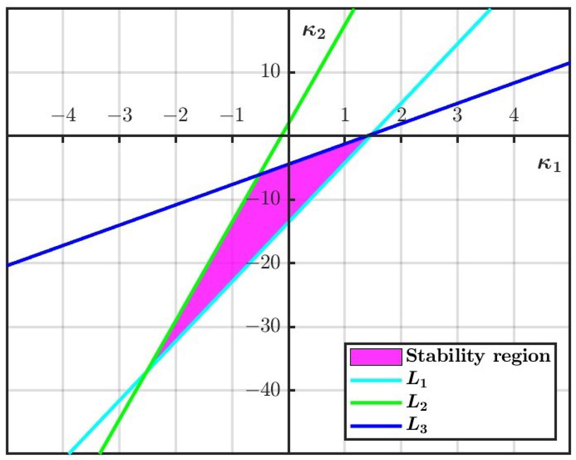
where $L_{30}=4+{\displaystyle \frac{h^2(-1+\alpha )(-1+(-1+\alpha )\beta )}{\alpha }}+{\displaystyle \frac{2h(1+{(-1+\alpha )}^2\beta -{\alpha }^2\gamma )}{\alpha (-1+\alpha \gamma )}}$. The region of stability is given by the triangular domain enclosed by $L_1$, $L_2$, and $L_3$.

The triangular region delineates the set of parameter pairs $({\kappa }_1,{\kappa }_2)$ for which the controlled system remains stable. Choosing $({\kappa }_1,{\kappa }_2)$ in this range will cause the appropriate eigenvalues to move into the interior of the unit circle, thus making the equilibrium point stable. In biological terms, this may be understood as adjusting the regulation of the bacteria and nutrient levels such that undesirable oscillations are eliminated and stability is achieved.

Afterward, we apply the technique of using a hybrid control methodology [22], which combines state feedback and parameter manipulation for achieving stability of the system. This will be done through introducing the control parameter $\rho \in (0,1)$, which basically acts as an interpolation between the uncontrolled and controlled system. The advantage of applying this method comes from its flexibility because by controlling this parameter, we will be able to steer the system toward stability in a conditionally stable manner. The controlled system is expressed by

$$\left\{\begin{array}{c}{x}_{n+1}=\rho \left(x_n+h\left({\displaystyle \frac{\alpha x_n{y}_n}{1+y_n}}-x_n\right)\right)+(1-\rho )x_n,\hfill \\ y_{n+1}=\rho \left(y_n+h\left(-{\displaystyle \frac{x_n{y}_n}{1+y_n}}-y_n+\beta +\gamma x_n\right)\right)+(1-\rho )y_n,\hfill \end{array}\right.$$

(39)

where $0<\rho <1$ is the control parameter. Both system (39) and system (3) possess identical fixed points. It is obtained that

$$J\left(E^{*}\right)=\left[\begin{array}{cc}1& -{\displaystyle \frac{h(-1+\alpha )(-1+(-1+\alpha \left)\beta \right)\rho }{-1+\alpha \gamma }}\\ {\displaystyle \frac{h(-1+\alpha \gamma )\rho }{\alpha }}& 1+{\displaystyle \frac{h(1+{(-1+\alpha )}^2\beta -{\alpha }^2\gamma )\rho }{\alpha (-1+\alpha \gamma )}}\end{array}\right],$$

(40)

then, its characteristic equation is given by

$${\xi }^2+K_1\xi +K_0=0,$$

(41)

where

$$\begin{array}{cc}\hfill K_1& ={\displaystyle \frac{-h(1+\beta )\rho +2\alpha (1+h\beta \rho )+{\alpha }^2(-h\beta \rho +\gamma (-2+h\rho ))}{\alpha (-1+\alpha \gamma )}},\hfill \\ \hfill K_0& ={\displaystyle \frac{1}{\alpha (-1+\alpha \gamma )}}(h^2{\alpha }^3\beta \gamma {\rho }^2-h(1+\beta )\rho (-1+h\rho )+\alpha (-1-2h\beta \rho +h^2(1+\gamma +\beta (2+\gamma )){\rho }^2)\hfill \\ \hfill & -{\alpha }^2(h\beta \rho (-1+h\rho )+\gamma (-1+h\rho +h^2(1+2\beta ){\rho }^2))).\hfill \end{array}$$

When $|K_1|<1+K_0<2$, there is a sink at the fixed point $E^{*}$ of (39). Therefore, one can control the stability of the equilibrium point of coexistence $E^{*}$ using the parameter $\rho$. It is possible to force the eigenvalues of the system (39) to lie within the unit circle by setting $\rho$.

Remark 1. 

Besides the state feedback and hybrid control strategies considered above, other approaches, such as parameter perturbation, adaptive control, delayed feedback control, and impulsive control, may also be employed to suppress undesirable oscillations and chaotic dynamics in discrete-time systems. For the corresponding continuous-time system (2), control can be introduced through biologically accessible quantities such as the nutrient input, dilution rate, or recycling rate. For example, feedback or adaptive control may be designed to regulate these quantities and drive the system toward a desired equilibrium. In the present model, however, the positive equilibrium of the continuous system is already locally asymptotically stable under its existence conditions. Therefore, the control strategies used here are primarily relevant to stabilizing the complex dynamics arising in the discrete-time model.

6. Numerical Examples

In this section, we present numerical simulations to complement and illustrate the analytical results. These confirm the theoretical results on stability and bifurcation, and they also reveal more intricate behaviors, including periodic oscillations and chaos. All calculations are carried out in Mathematica 13.3, while the figures are produced using MATLAB R2023a.

6.1. Transcritical Bifurcation Analysis

Assume that $\alpha =1.6$, $\gamma =0.4$, and $h=1.3$. With these parameter values, the boundary fixed point is $E_1=(0,1.66667)$. The system (3) goes through a transcritical bifurcation at $E_1$ when ${\beta }_1=1.66667$. At this critical value, the eigenvalues of $J\left(E_1\right)$ are ${\xi }_1=1$ and ${\xi }_2=-0.3$. This indicates that the fixed point is non-hyperbolic.

Furthermore, the reduced map on the center manifold is given by

$$\begin{array}{cc}\hfill \mathrm{\Phi }({\mu }_n,ϵ)& ={\mu }_n+0.2925{\mu }_n^2+0.2925{\mu }_nϵ+0.0073125{\mu }_n^3-0.102375{\mu }_n^2ϵ-0.109688{\mu }_n{ϵ}^2,\hfill \end{array}$$

and satisfies

$$\begin{array}{c}\hfill \mathrm{\Phi }(0,0)=0,{\mathrm{\Phi }}_{{\mu }_n}(0,0)=1,{\mathrm{\Phi }}_{ϵ}(0,0)=0,\\ \hfill {\mathrm{\Phi }}_{{\mu }_n{\mu }_n}(0,0)=0.585\ne 0,{\mathrm{\Phi }}_{{\mu }_nϵ}(0,0)=0.2925\ne 0,\end{array}$$

which verifies the conditions of Theorem 3 and confirms the occurrence of a transcritical bifurcation.

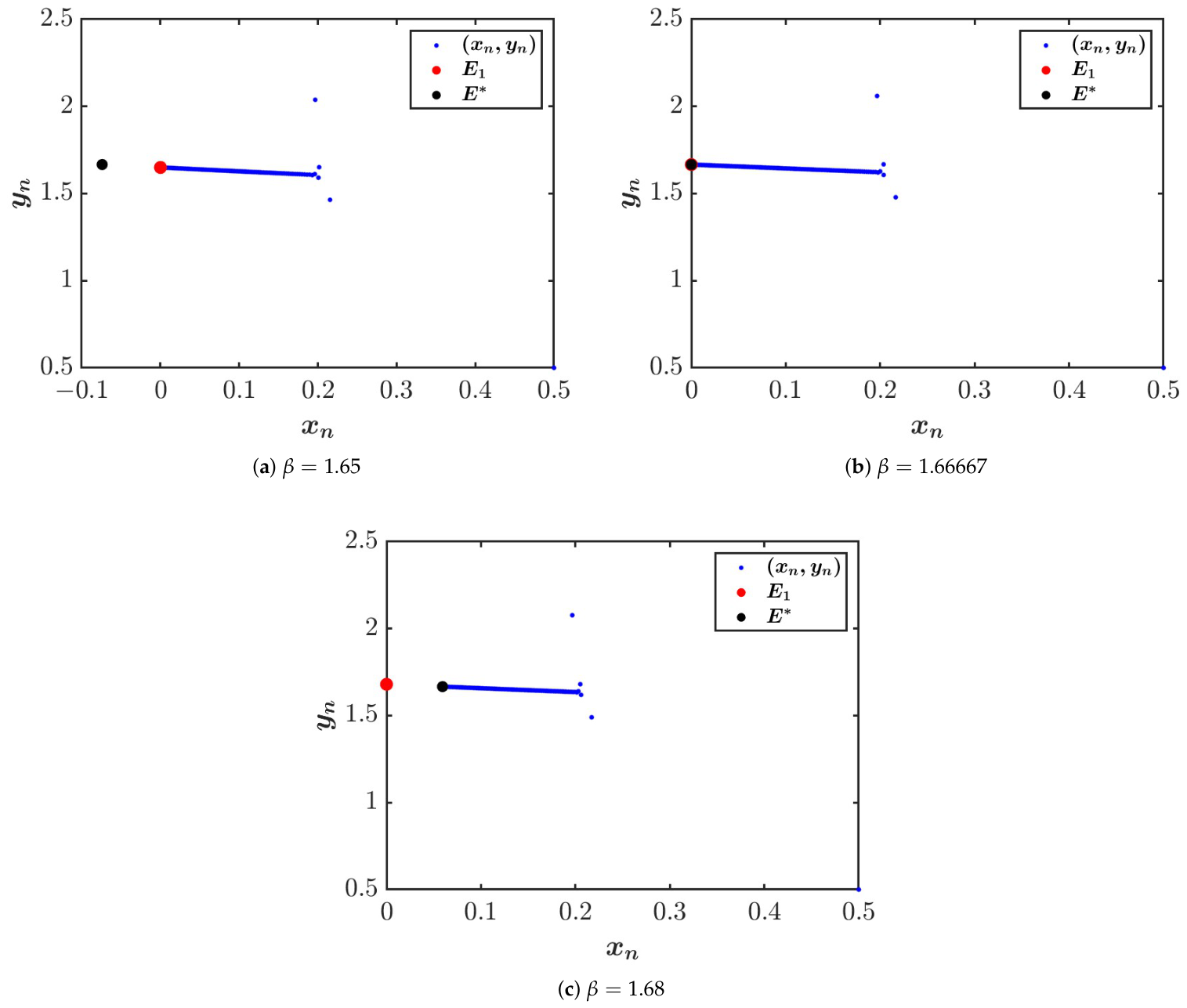
To illustrate this behavior, phase portrait diagrams are provided in Figure 1. Biologically, the equilibrium $E^{*}$ does not make sense when $\beta \le 1.66667$, because the population level of bacteria becomes non-positive. For $\beta =1.65$, as seen from Figure 1a, $E_1$ is stable but $E^{*}$ is unstable, showing extinction of bacteria. At the threshold parameter value $\beta =1.66667$, we notice that Figure 1b illustrates collision and switching of stability of the two equilibria $E_1$ and $E^{*}$. If $\beta$ surpasses this threshold value, say $\beta =1.68$, then Figure 1c indicates that the stability of $E^{*}$ switches to stability, whereas that of $E_1$ switches to instability, which means the appearance of a coexistence state. This exchange of stability between $E_1$ and $E^{*}$ clearly confirms the presence of a transcritical bifurcation in the system.

6.2. Period-Doubling Bifurcation Analysis

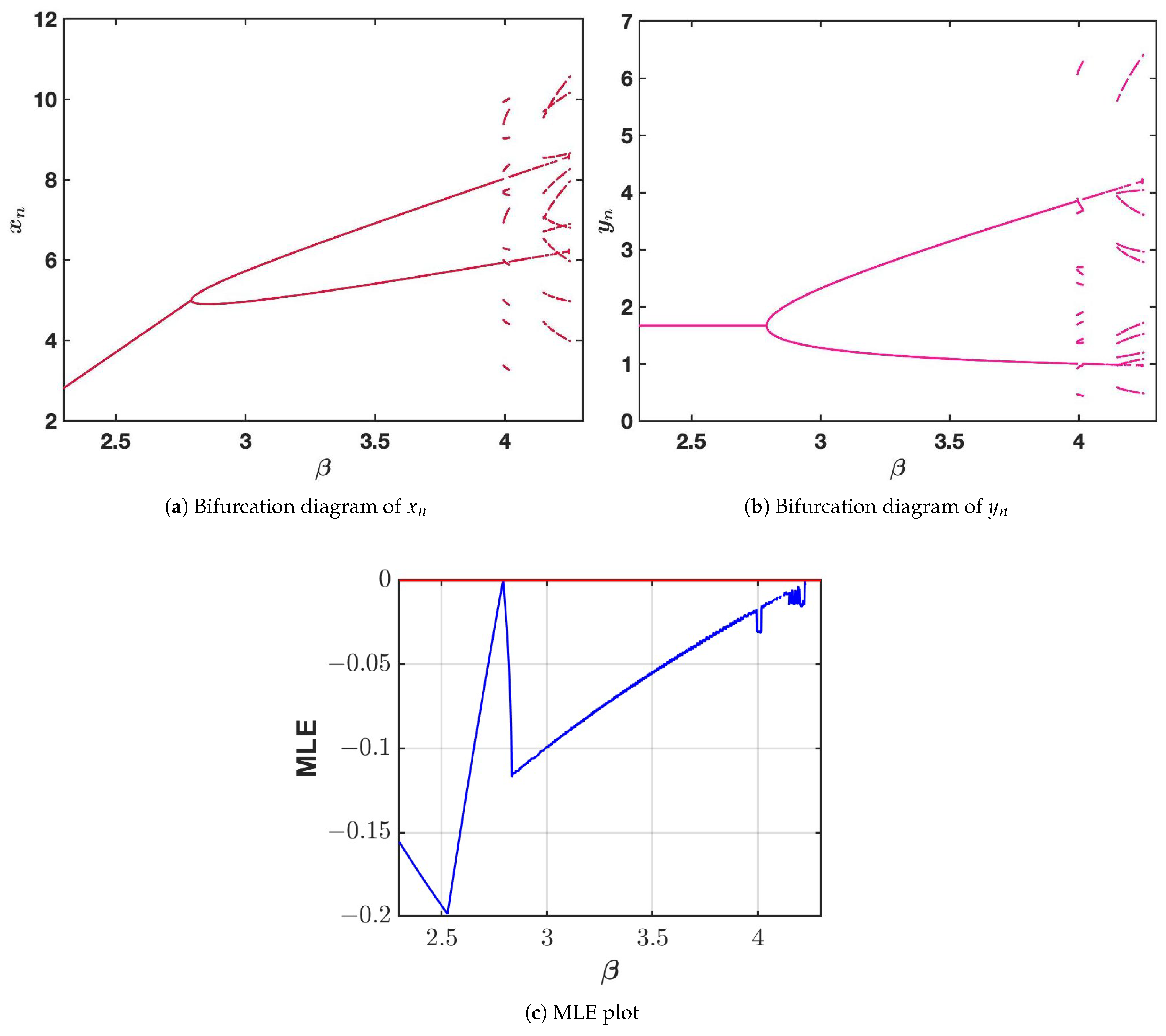
We set $\alpha =1.6$, $\gamma =0.4$, and $h=1.3$. With these parameter values, the system (3) experiences a period-doubling bifurcation at ${\beta }_2=2.79139$. The related positive fixed point is $E^{*}=(4.99877,1.66667)$. At this critical value, the eigenvalues of $J\left(E^{*}\right)$ are ${\xi }_1=-1$ and ${\xi }_2=0.786162$. This shows that one eigenvalue crosses $-1$, which confirms the period-doubling bifurcation noted in Theorem 5.

Additionally, the resulting values for the coefficients are $l_1=-1.39377\ne 0$ and $l_2=1.15242\ne 0$, indicating that all theoretical necessary conditions have been met. Because $l_2>0$, this produces a stable period-2 cycle emanating from $E^{*}$, which means that there is a transition between steady-state coexistence and oscillatory dynamics.

In order to illustrate this dynamical behavior, bifurcation diagrams against $\beta$ are depicted in Figure 2a,b in the range $\beta \in [2.3,4.3]$. It is evident from these figures that when the control parameter exceeds a certain threshold value ${\beta }_2$, the system undergoes a period-doubling bifurcation and generates a stable period-2 cycle. In this case, the MLE of the model is shown in Figure 2c. Therefore, one can observe that higher nutrient input may induce instability in the system.

Next, we choose $\alpha =1.6$, $\beta =2.5$, and $h=1.3$. Under this choice of parameters, the system undergoes a period-doubling bifurcation at $\gamma =0.447534$. The corresponding positive equilibrium is $E^{*}=(4.69573,1.66667)$. At this critical point, the eigenvalues of $J\left(E^{*}\right)$ are ${\xi }_1=-1$ and ${\xi }_2=0.841562$, showing that one eigenvalue crosses $-1$, which confirms the onset of period-doubling bifurcation as described in Theorem 5.

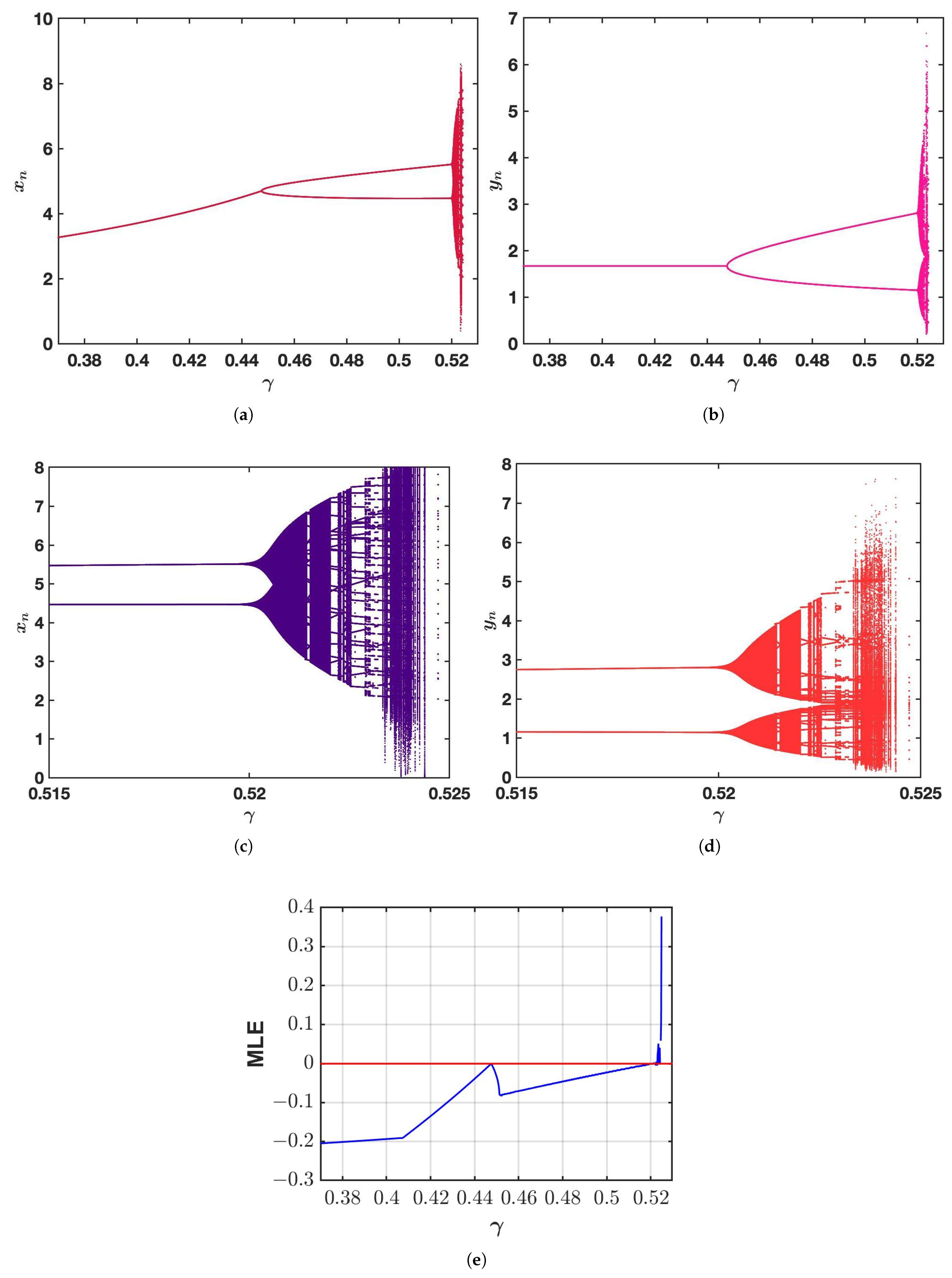
Bifurcation diagrams with respect to $\gamma$ are shown in Figure 3a,b for $\gamma \in [0.37,0.53]$. These bifurcation diagrams reveal the existence of the period doubling phenomenon when $\gamma \ge 0.447534$ and hence, the equilibrium point $E^{*}$ becomes unstable while a stable periodic orbit of period-2 arises. A magnified view of the bifurcation structure on $\gamma \in [0.515,0.525]$ is provided in Figure 3c,d, which further reveals a cascade of period-doubling bifurcations and the onset of more intricate dynamical behavior. Figure 3e shows the corresponding MLE curve. The negative value of MLE means that periodic oscillations are stable, whereas the MLE equal to zero means bifurcation. Further increase in parameter $\gamma$ leads to positive MLE, indicating chaos.

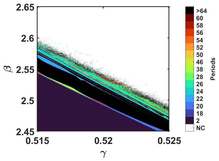
To further investigate the combined influence of the nutrient input rate $\beta$ and the recycling rate $\gamma$, a two-parameter bifurcation diagram is presented in Figure 4. Here, $\alpha =1.6$ and $h=1.3$ are fixed, while $\gamma \in [0.515,0.525]$ and $\beta \in [2.45,2.65]$ are varied simultaneously. The diagram reveals a highly structured organization of periodic windows in the $(\gamma ,\beta )$ parameter plane. In particular, regions corresponding to periodic orbits of different periods are arranged in narrow bands, showing that small simultaneous variations in the nutrient supply and recycling rates can produce substantial changes in the long-term dynamics. The occurrence of successively higher-period regions is consistent with the complex bifurcation structure observed in the one-parameter diagrams.

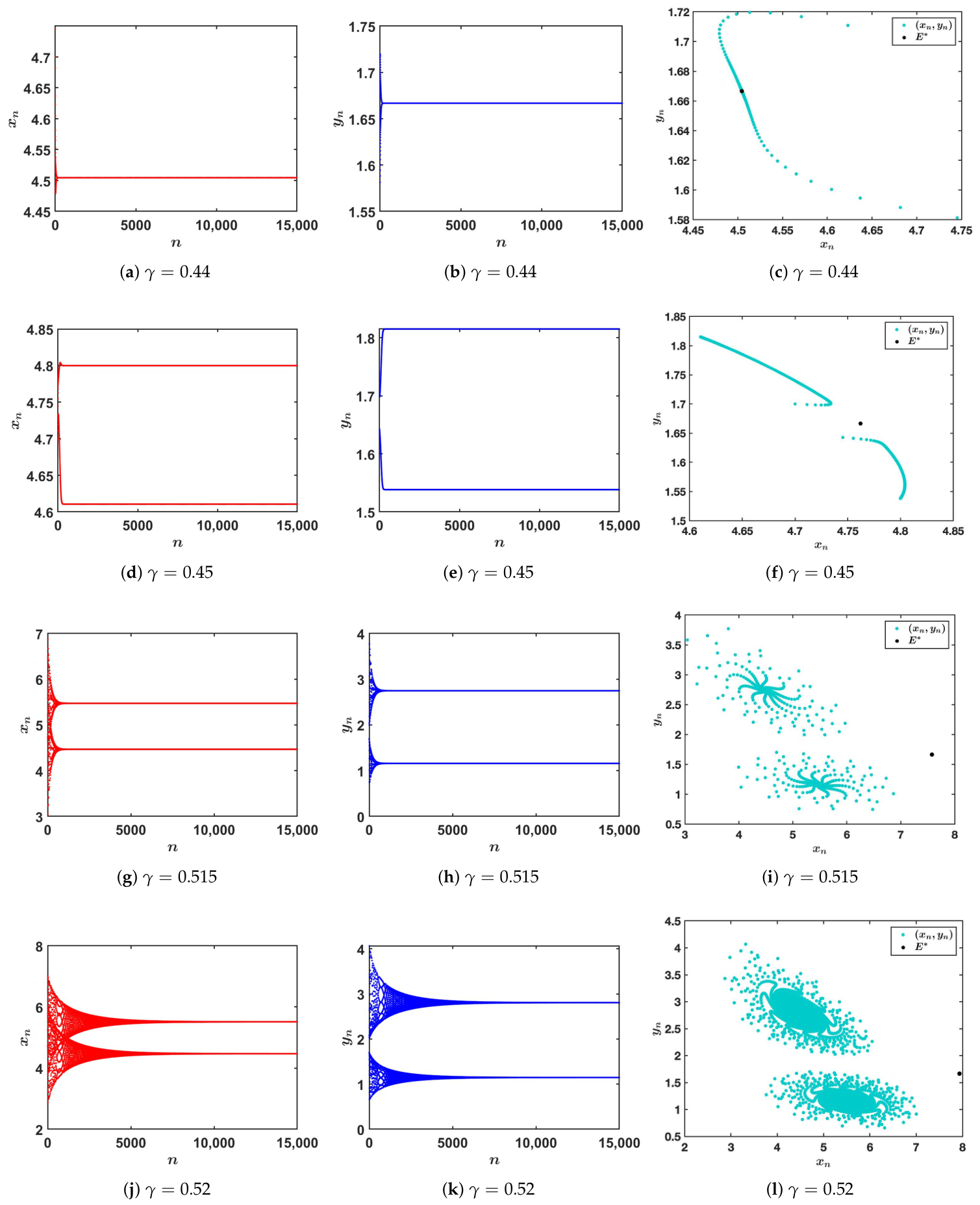
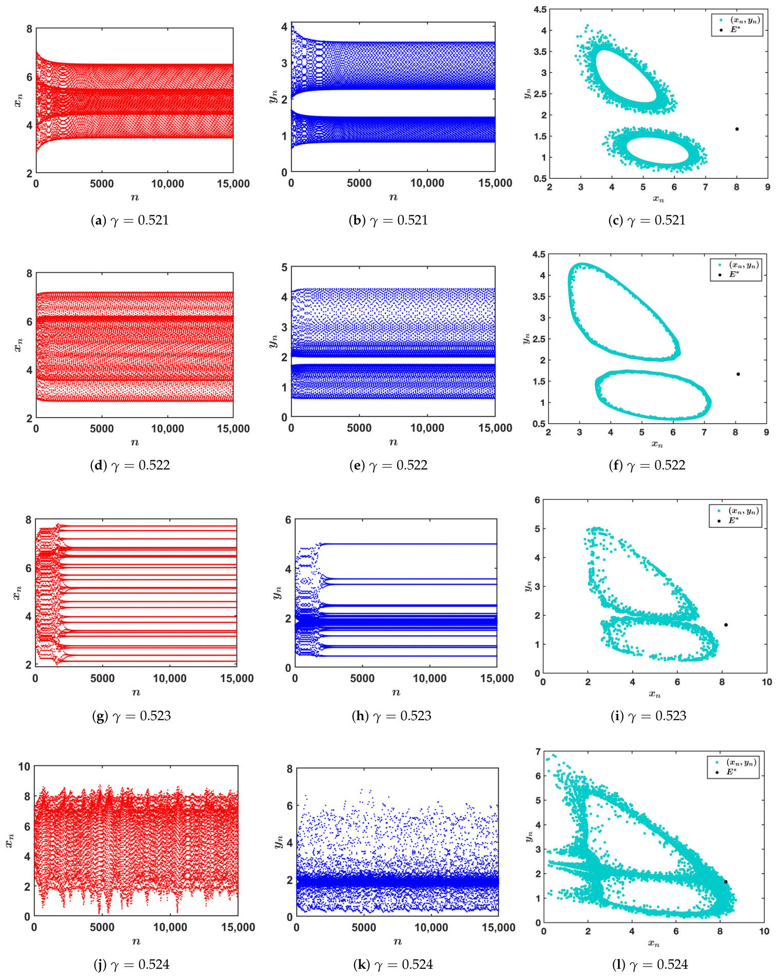
The dynamical alterations are further described by the phase portraits in Figure 5 and Figure 6. For $\gamma =0.44$, $E^{*}$ is stable, indicating steady coexistence between bacteria and nutrients. Once $\gamma$ crosses the critical threshold $\gamma =0.447534$, the equilibrium loses stability and a stable period-2 orbit appears, as seen for $\gamma =0.45$. As $\gamma$ increases further, the system undergoes a cascade of period-doubling bifurcations, yielding progressively more intricate oscillatory patterns. For larger values, such as $\gamma =0.524$, the dynamics become chaotic, with trajectories that are irregular, aperiodic, and highly sensitive to initial conditions.

Biologically, this result brings to attention the importance of the nutrient recycling rate $\gamma$. Moderate nutrient recycling ensures high nutrient levels that enable stable coexistence of species. On the other hand, high nutrient recycling can cause destabilization, leading to dramatic oscillatory dynamics in the population and nutrient density.

6.3. Influence of the Step Size on Bifurcation Thresholds

Since system (3) is obtained using the forward Euler scheme, the step size h directly influences the discrete stability and bifurcation conditions. The forward Euler method has a local truncation error of $O\left(h^2\right)$ and a global error of $O\left(h\right)$. Therefore, the bifurcation thresholds of the discrete system may depend on the selected finite step size. Indeed, the period-doubling threshold ${\beta }_2$ obtained in Theorem 5 depends explicitly on h, showing that changes in h shift the corresponding bifurcation boundary. Numerical bifurcation diagrams with respect to h are presented below to further illustrate the influence of the discretization step on the system dynamics.

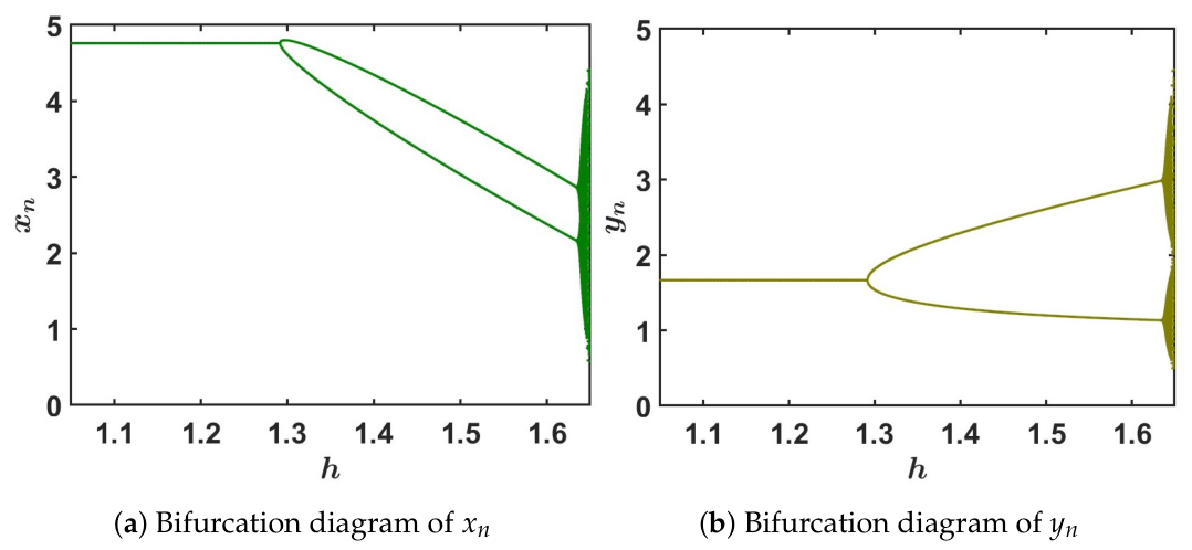
To examine the influence of the forward Euler step size on the dynamics, we fix $\alpha =1.6,\beta =2.5,\gamma =0.45,$ and vary h. For these parameter values, the critical step size for the period-doubling bifurcation is $h=1.29152$. The corresponding positive fixed point is $E^{*}=(4.7619,1.66667)$, and the eigenvalues of $J\left(E^{*}\right)$ are ${\xi }_1=-1$ and ${\xi }_2=0.843623$, confirming the period-doubling condition.

Figure 7 shows the bifurcation diagrams of $x_n$ and $y_n$ with respect to h. For $h<1.29152$, trajectories converge to the positive equilibrium. As h crosses $1.29152$, a stable period-2 orbit emerges. Thus, the numerical results confirm the analytical dependence of the discrete dynamics on the Euler step size. In particular, larger finite step sizes can destabilize the equilibrium and alter the location of the bifurcation boundaries.

Moreover,

Table 1. Variation of the critical period-doubling threshold ${\beta }_2$ with the Euler step size h.

h	Critical Value ${\mathit{\beta }}_2$	h	Critical Value ${\mathit{\beta }}_2$
0.1	25.6468	0.9	3.40693
0.2	13.1893	1.0	3.1137
0.3	9.02768	1.1	2.87019
0.4	6.93974	1.2	2.66382
0.5	5.681	1.3	2.48584
0.6	4.83665	1.4	2.33002
0.7	4.22887	1.5	2.19175
0.8	3.76877	1.6	2.06758

reports the critical values of ${\beta }_2$ obtained for different values of h, while the remaining parameters are kept fixed as $\alpha =1.6$ and $\gamma =0.45$. It demonstrates a clear shift in the period-doubling threshold as the Euler step size is varied. Thus, increasing h shifts the period-doubling boundary toward smaller values of $\beta$, whereas decreasing h shifts it toward larger values.

6.4. Basins of Attraction and Multistability

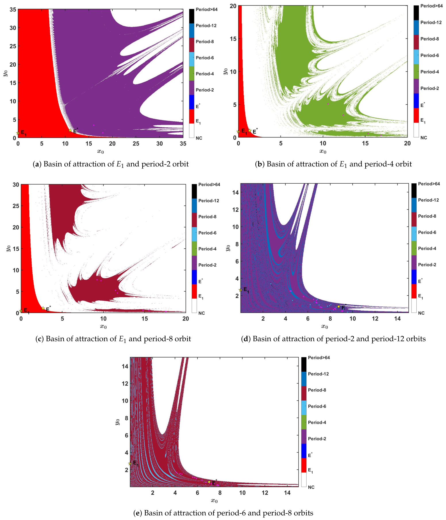
To further investigate the global dynamics of system (3), the basins of attraction associated with different coexisting attractors are examined. Unlike one- and two-parameter bifurcation diagrams, which describe changes in the asymptotic dynamics as model parameters vary, basin diagrams reveal the dependence of long-term behavior on the initial conditions $(x_0,y_0)$ for fixed parameter values. In each diagram, a grid of initial conditions is iterated under system (3), with each initial condition classified according to the attractor approached by the corresponding trajectory. The resulting basin structure thus provides a direct visualization of multistability and the sensitivity of the asymptotic dynamics to the choice of initial conditions.

Figure 8a–e illustrate the basins of attraction of system (3) and reveal the presence of multistability for different parameter sets given in

Table 2. Parameter values used for basin of attraction plots.

Figure	Parameter Values
Figure 8a	$\alpha =1.50,\beta =1.30,\gamma =0.73,h=0.74.$
Figure 8b	$\alpha =1.98,\beta =0.88,\gamma =0.61,h=0.684.$
Figure 8c	$\alpha =1.97,\beta =0.455,\gamma =0.723,h=0.812.$
Figure 8d	$\alpha =2.374,\beta =2.651,\gamma =0.2014,h=0.861.$
Figure 8e	$\alpha =2.736,\beta =2.711,\gamma =0.0623,h=0.890.$

. In particular, the coexistence of the boundary equilibrium $E_1$ with period-2, period-4, and period-8 attractors is observed, while other parameter choices exhibit coexistence between period-2 and period-12 attractors and between period-6 and period-8 attractors. The distinct and intricately structured basins demonstrate that, for the same parameter values, different initial conditions may lead to qualitatively different long-term behaviors. Thus, the basin analysis complements the bifurcation diagrams and phase portraits by showing that the asymptotic dynamics depend not only on the model parameters but also strongly on the initial state. Biologically, this multistability implies that identical environmental conditions may result in different long-term bacteria-nutrient dynamics, ranging from bacterial extinction to persistent oscillatory regimes, depending on the initial bacterial and nutrient concentrations.

6.5. Chaos Control Examples

Let us analyze the efficacy of the control approaches presented for stabilization of the system dynamics. To begin with, we analyze the state feedback control technique. By employing the parameters $\alpha =1.6$, $\beta =2.5$, $\gamma =0.5$, and $h=1.3$, the marginal stability lines for the controlled system (31) are determined as

$$\begin{array}{c}\hfill L_1:{\kappa }_2=9.34615{\kappa }_1-13.55,L_2:{\kappa }_2=15.5{\kappa }_1+1.95,L_3:{\kappa }_2={\kappa }_1-4.43462.\end{array}$$

The stability region bounded by these lines is depicted in Figure 9, which gives the range of acceptable values for feedback gains $({\kappa }_1,{\kappa }_2)$ to ensure local stability of the controlled system.

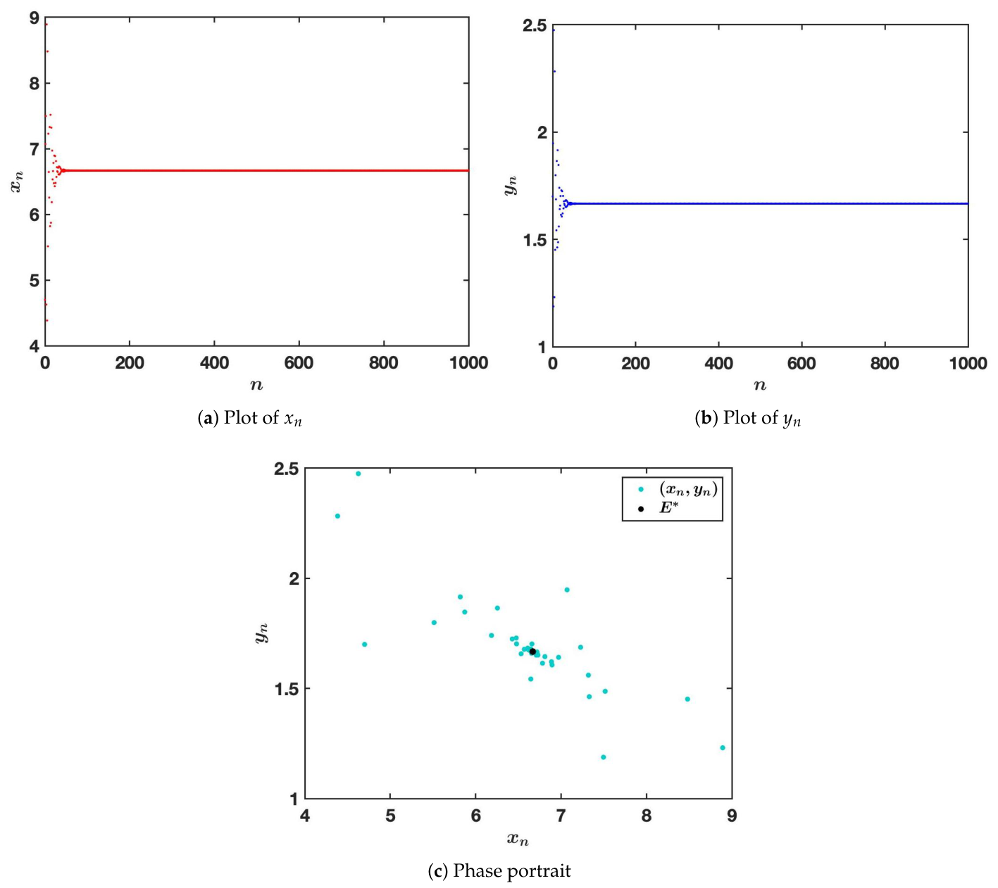
Under these parameter conditions, the positive fixed point $E^{*}=(6.66667,1.66667)$ of the system (3) is unstable. For this equilibrium point to become stable, we use the control force $U_n={\kappa }_1(x_n-6.66667)+{\kappa }_2(y_n-1.66667)$, where ${\kappa }_1=1.16$ and ${\kappa }_2=-1.31$ belong to the stability region. The time series plots of $x_n$ and $y_n$ are shown in Figure 10a and Figure 10b, respectively, while the associated phase portrait is given in Figure 10c. From these graphs, it is clear that the feedback control method suppresses oscillations and stabilizes the system at the desired equilibrium without chaotic and period-doubling behavior.

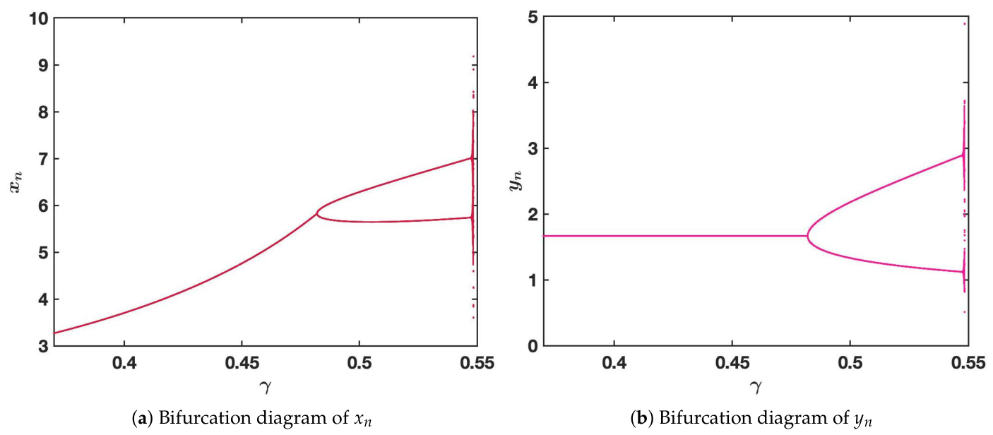
We now analyze the efficacy of the hybrid control scheme. For the controlled system (39), the parameters are fixed as $\rho =0.9$, $\alpha =1.6$, $\beta =2.5$, and $h=1.3$, while $\gamma$ is varied. The bifurcation diagrams shown in Figure 11 reveal that the period-doubling bifurcation occurs at $\gamma =0.48193$, which is higher than the corresponding bifurcation value for the uncontrolled system (3). This shift indicates that the hybrid control strategy delays the onset of instability and expands the range of parameter values over which the system remains stable.

From a biological point of view, these control strategies can be interpreted as regulatory mechanisms to stabilize the dynamics of populations. In contrast, the feedback control approach compensates for deviations from equilibrium by controlling the system actively while the hybrid control approach controls the system indirectly through a weighted sum of controlled dynamics and uncontrolled open-loop dynamics. Both approaches result in suppressing unwanted oscillations, yielding stable coexistence mechanics between bacteria and carbon sources.

7. Conclusions

This study proposed and investigated a novel discrete-time chemostat model with nutrient recycling. By adding the recycling parameter, the classical model is improved in such a way that it considers the internal feedback process caused by the regeneration of nutrients by biomass. The addition of the recycling parameter makes the ecological interaction more practical and also makes the dynamics of the system richer. Two meaningful equilibria of the system are obtained, and the stability conditions for both the equilibria are explicitly calculated by linearization and characteristic equations.

The bifurcation analysis reveals that the system undergoes both transcritical and period-doubling bifurcations. The transcritical bifurcation describes the transition from extinction to persistence as nutrient input crosses a critical threshold, and the period-doubling bifurcation points to the onset of oscillatory and potentially chaotic dynamics. Also, it is proved that there is no Neimark–Sacker bifurcation in this model. These analytical results are strongly supported by numerical simulations and clearly show the emergence of complex dynamics as parameters in the system change.

In comparison with existing chemostat models, the present model provided a broader description by incorporating nutrient recycling into a discrete-time framework and examining its interaction with discretization. In the continuous-time framework of [3], nutrient recycling was incorporated with mutualistic bacterial interactions, with emphasis on positivity, boundedness, coexistence, stability, persistence, and control. In contrast, the discrete chemostat model in [8] exhibited fold, period-doubling, Neimark–Sacker, and $R_4$ resonance bifurcations but did not include nutrient recycling. Alsulami [10] considered a chemostat model without nutrient recycling and discretized it using the piecewise constant argument method, which preserved non-negativity and produced transcritical and period-doubling bifurcations. In contrast, the present model incorporated the recycling term and employed forward Euler discretization, so that both the recycling parameter $\gamma$ and the step size h directly affect the stability and bifurcation conditions. Unlike [8], the present model exhibited period-doubling and complex dynamics while analytically excluding a Neimark–Sacker bifurcation at the positive equilibrium.

The proposed two-dimensional framework can be extended to higher-dimensional chemostat models by incorporating additional biologically relevant variables. For example, a three-dimensional model may include bacterial biomass, nutrient concentration, and recycled organic matter, while a four-dimensional model may further incorporate a competing microbial population. Such extensions could provide a more realistic description of nutrient recycling in complex microbial communities and constitute an interesting direction for future research. Future studies may also consider time delays, stochastic effects, and alternative positivity-preserving discretization schemes to examine their influence on the stability and bifurcation structure.

References

1. Santiago-Rodriguez, T.M.; Ly, M.; Daigneault, M.C.; Brown, I.H.L.; McDonald, J.A.K.; Bonilla, N.; Vercoe, E.A.; Pride, D.T. Chemostat culture systems support diverse bacteriophage communities from human feces. Microbiome 2025, 3, 58. [Google Scholar] [CrossRef] [Scilit] [PubMed]
2. Spagnolo, F.; Caballero, I.; Goldblatt, A.; Loccisano, M.J.; Mahe, M.I.; Mejia, Y.; Melvani, N.; Nagel, A.; Stanciu, A.; Kannoly, S.; et al. A chemostat-based model for growing bacterial biofilms. Microbiol. Spectr. 2025, 13, e02333-25. [Google Scholar] [CrossRef] [Scilit] [PubMed]
3. Alalhareth, F.K.; Aljohani, A.R.; Alharbi, M.H.; Hajji, M.E. Modeling, stability analysis, and optimal control of a chemostat model for mutualistic bacterial species with leachate recycling. AIMS Math. 2025, 10, 28714–28752. [Google Scholar] [CrossRef] [Scilit]
4. Pilyugin, S.S.; Waltman, P. Multiple limit cycles in the chemostat with variable yield. Math. Biosci. 2003, 182, 151–166. [Google Scholar] [CrossRef] [Scilit] [PubMed]
5. Mazenc, F.; Malisoff, M. Stability and stabilization for models of chemostats with multiple limiting substrates. J. Biol. Dyn. 2012, 6, 612–627. [Google Scholar] [CrossRef] [Scilit] [PubMed]
6. Khan, Z.A.; Shah, K.; Abdalla, B.; Abdeljawad, T. A numerical study of complex dynamics of a chemostat model under fractal-fractional derivative. Fractals 2023, 31, 2340181. [Google Scholar] [CrossRef] [Scilit]
7. Ali, N.B.; Abdellatif, N. Stability and bifurcations in a model of chemostat with two inter-connected inhibitions and a negative feedback loop. Math. Methods Appl. Sci. 2025, 48, 658–677. [Google Scholar] [CrossRef] [Scilit]
8. Sharma, V.S.; Mangal, S.; Singh, A. A complex dynamics of discrete-time chemostat model: Codimension-one and two bifurcations analysis. J. Appl. Math. Comput. 2025, 71, 8767–8794. [Google Scholar] [CrossRef] [Scilit]
9. Al-Basyouni, K.S.N.; Khan, A.Q. Bifurcation analysis of a discrete-time chemostat model. Math. Probl. Eng. 2023, 2023, 7518261. [Google Scholar] [CrossRef] [Scilit]
10. Alsulami, I.M. On the stability, chaos and bifurcation analysis of a discrete-time chemostat model using the piecewise constant argument method. AIMS Math. 2024, 9, 33861–33878. [Google Scholar] [CrossRef] [Scilit]
11. Strogatz, S.H. Nonlinear Dynamics and Chaos: With Applications to Physics, Biology, Chemistry, and Engineering, 2nd ed.; CRC Press: Boca Raton, FL, USA, 2018. [Google Scholar] [CrossRef] [Scilit]
12. Chong, Y.; Kashyap, A.J.; Chen, S.; Chen, F. Dynamics analysis of a discrete-time commensalism model with additive Allee for the host species. Axioms 2023, 12, 1031. [Google Scholar] [CrossRef] [Scilit]
13. Ahmed, R.; Khan, A.Q.; Amer, M.; Faizan, A.; Ahmed, I. Complex dynamics of a discretized predator-prey system with prey refuge using a piecewise constant argument method. Int. J. Bifurc. Chaos 2024, 34, 2450120. [Google Scholar] [CrossRef] [Scilit]
14. Almatrafi, M.B.; Berkal, M.; Ahmed, R. Dynamical transitions and chaos control in a discrete predator-prey model with Gompertz growth and Holling type III response. Chaos Solitons Fractals 2025, 200, 117071. [Google Scholar] [CrossRef] [Scilit]
15. Ahmed, R.; Yazdani, M.S. Complex dynamics of a discrete-time model with prey refuge and Holling type-II functional response. J. Math. Comput. Sci. 2022, 12, 113. [Google Scholar] [CrossRef] [Scilit]
16. Tassaddiq, A.; Mehmood, A.; Ahmed, R. Impact of carrying capacity on the dynamics of a discrete-time plant-herbivore system. Chaos Solitons Fractals 2025, 201, 117284. [Google Scholar] [CrossRef] [Scilit]
17. Guckenheimer, J.; Holmes, P. Nonlinear Oscillations, Dynamical Systems, and Bifurcations of Vector Fields; Springer: New York, NY, USA, 1983; Volume 42. [Google Scholar] [CrossRef] [Scilit]
18. Wiggins, S.; Golubitsky, M. Introduction to Applied Nonlinear Dynamical Systems and Chaos; Springer: Berlin/Heidelberg, Germany, 2003; Volume 2. [Google Scholar] [CrossRef] [Scilit]
19. Kuznetsov, Y.A. Elements of Applied Bifurcation Theory; Springer: New York, NY, USA, 2004; Volume 112. [Google Scholar] [CrossRef] [Scilit]
20. Chen, G.; Dong, X. From Chaos to Order: Methodologies, Perspectives and Applications; World Scientific: Singapore, 1998; Volume 24. [Google Scholar] [CrossRef]
21. Lei, C.; Han, X.; Wang, W. Bifurcation analysis and chaos control of a discrete-time prey-predator model with fear factor. Math. Biosci. Eng. 2022, 19, 6659–6679. [Google Scholar] [CrossRef] [Scilit] [PubMed]
22. Luo, X.S.; Chen, G.; Wang, B.H.; Fang, J.Q. Hybrid control of period-doubling bifurcation and chaos in discrete nonlinear dynamical systems. Chaos Solitons Fractals 2003, 18, 775–783. [Google Scholar] [CrossRef] [Scilit]
Figure 1. Phase portraits of the system (3) showing the transcritical bifurcation with respect to β . Fixed parameter values are α = 1.6 ,   γ = 0.4 ,   h = 1.3 ,   and initial conditions are x 0 = 0.5 ,   y 0 = 0.5 .
Mathematics 14 03398 g001
Figure 2. Bifurcation diagrams and MLE plot of (3) varying β . Fixed parameter values are α = 1.6 , γ = 0.4 ,   h = 1.3 ,   and initial conditions are x 0 = 4.9 ,   y 0 = 1.7 .
Mathematics 14 03398 g002
Figure 3. Bifurcation diagrams and MLE plot of (3) varying γ . Fixed parameter values are α = 1.6 , β = 2.5 ,   h = 1.3 ,   and initial conditions are x 0 = 4.7 ,   y 0 = 1.7 .
Mathematics 14 03398 g003
Figure 4. Bifurcation diagram of system (3) in ( γ ,   β ) –plane by varying γ [ 0.515 ,   0.525 ] and β [ 2.45 ,   2.65 ] . Fixed parameter values are α = 1.6 and h = 1.3 with initial values x 0 = 4.7 and y 0 = 1.7 . Colors indicate the detected periodicities, > 64 denotes parameter values for which no period up to 64 was detected, while NC denotes cases for which the numerical iteration does not converge.
Mathematics 14 03398 g004
Figure 5. Time series plots and phase portraits of (3) for γ { 0.44 ,   0.45 ,   0.515 ,   0.52 } and fixing α = 1.6 ,   β = 2.5 ,   h = 1.3 , x 0 = 4.7 , y 0 = 1.7 .
Mathematics 14 03398 g005
Figure 6. Time series plots and phase portraits of (3) for γ { 0.521 ,   0.522 ,   0.523 ,   0.524 } and fixing α = 1.6 ,   β = 2.5 ,   h = 1.3 , x 0 = 4.7 , y 0 = 1.7 .
Mathematics 14 03398 g006
Figure 7. Bifurcation diagrams of (3) varying h [ 1.05 ,   1.65 ] . Fixed parameter values are α = 1.6 , β = 2.5 , γ = 0.45 ,   and initial conditions are x 0 = 4.7 ,   y 0 = 1.7 .
Mathematics 14 03398 g007
Figure 8. Basins of attraction of system (3) for different parameter sets given in Table 2, illustrating the coexistence of multiple attractors.
Mathematics 14 03398 g008
Figure 9. Stability region for the controlled model (31) with α = 1.6 ,   β = 2.5 ,   γ = 0.5 ,   h = 1.3 .
Mathematics 14 03398 g009
Figure 10. Time series plots and phase portrait of (31) with α = 1.6 ,   β = 2.5 ,   γ = 0.5 ,   h = 1.3 , κ 1 = 1.16 , κ 2 = 1.31 , x 0 = 4.7 ,   y 0 = 1.7 .
Mathematics 14 03398 g010
Figure 11. Bifurcation diagram of model (39) varying γ in [ 0.37 ,   0.55 ] . Fixed parameter values are ρ = 0.9 ,   α = 1.6 ,   β = 2.5 ,   h = 1.3 ,   and initial conditions are x 0 = 4.7 ,   y 0 = 1.7 .
Mathematics 14 03398 g011