Chaotic-Saddle-Organized Hidden Bursting Oscillations in a 4D Slow–Fast System with No Equilibria

Abstract

Bursting oscillations, characterized by alternating quiescent and spiking states, are a fundamental class of nonlinear dynamics that play a crucial role in diverse scientific fields. Therefore, understanding the mechanisms that generate bursting is of both theoretical and practical importance. Bursting is typically studied as a class of self-excited or forced oscillations in classical slow–fast dynamics, with analysis relying on stable invariant sets and their bifurcations. In contrast to these cases, we extend the analysis to hidden bursting in a 4D slow–fast system with no equilibria using classical slow–fast decomposition. Specifically, we show how chaotic saddle dynamics in the fast subsystem organize the bursting mechanism. Bifurcation and basin analyses identify two symmetric chaotic saddle ranges between interior crises and the folds of limit cycles. When quiescent-to-spiking transitions fall within these ranges, chaotic saddles render the full system highly sensitive to parameters, acting as the organizing center for hidden bursting. By tuning the slow adaptation strength, we uncover three transition-path modes: lift-captured double-reversal (LCDR), lift-escape single-reversal (LESR), and direct-captured no-reversal (DCNR). These modes and their combinations classify the observed bursting patterns. These findings show that non-attracting invariant sets can affect bursting dynamics, offering a new perspective on bursting dynamics.

1. Introduction

In recent decades, hidden attractors have attracted considerable attention in nonlinear science. These are attractors whose basins of attraction do not intersect any neighborhood of an equilibrium point [1]. This distinguishes them from self-excited attractors, which can be located by trajectories starting from vicinities of unstable equilibria. Although its conceptual roots can be traced back to Hilbert’s 16th problem [2,3], the concept of hidden attractors was systematically introduced and formalized following the discovery of unpredicted chaotic attractors in Chua’s circuit [1,4,5,6,7,8,9], marking a significant paradigm shift in the classical theory of oscillations [10].

Generally, systems with no equilibria are a class of autonomous systems defined by the absence of equilibrium points. By definition, all bounded oscillations in such systems are necessarily hidden attractors [11]. A variety of such systems have been proposed to explore their complex dynamics, including hidden periodic cycles, hidden chaos, and hidden hyperchaos [12,13,14,15,16]. Recently, hidden bursting oscillations have also been reported in such systems. Zhang and Zeng constructed a simple Jerk-like system without equilibrium, revealing asymmetric coexisting hidden attractors and bursting oscillations [17]. Yan et al. proposed a four-dimensional memristive Hindmarsh–Rose neuron model with no equilibria that produces diverse hidden firing patterns, including periodic bursting, chaotic bursting, and transient chaotic bursting [18]. More recently, Zhang et al. designed a four-dimensional no-equilibrium chaotic system and experimentally verified its controlled periodic and chaotic bursting oscillations through circuit implementation [19]. Although these studies demonstrate that systems with no equilibria can serve as promising platforms for generating rich hidden bursting phenomena, the underlying dynamical mechanisms remain to be further elucidated.

In classical slow–fast dynamics, bursting oscillations are understood through the decomposition of the full system into fast and slow subsystems, known as the slow–fast decomposition method [20]. In this framework, the quiescent and spiking states correspond to stable equilibria and stable non-equilibrium invariant sets of the fast subsystem, respectively, with transitions between them induced by bifurcations as the slow variable sweeps across critical thresholds [21,22]. This framework has been extensively validated and extended over the past decades [23,24,25,26,27,28]. Zhang et al. further extended this framework to systems with slow external excitation by treating the excitation term as a generalized slow variable [29], and this modified method has been widely applied to reveal bursting mechanisms in such systems [30,31,32,33,34,35]. In this context, the slow–fast systems studied in previous works can be divided into two classes. The first class consists of systems with equilibria, where a clear timescale separation exists among the state variables. The bursting behaviors in these systems are a class of self-excited oscillations. The second class consists of systems with slow external excitation, where the bursting behaviors are a class of forced oscillations driven by the external excitation.

Despite the success of this framework, it focuses exclusively on stable invariant sets of the fast subsystem. However, non-attracting invariant sets, such as chaotic saddles, are ubiquitous in nonlinear dynamics. Unlike regular saddles, chaotic saddles possess a fractal structure of intertwined stable and unstable manifolds [36]. Trajectories near such sets exhibit transient chaos: finite-time chaotic behavior that eventually decays to a coexisting stable attractor. Whether such non-attracting sets can participate in the organization of bursting dynamics remains an open question. Recent work by Zhao et al. [37] demonstrated that chaotic saddles can organize chaotic bursting in a system with slow external excitation, where the trajectory is forced unidirectionally through the saddle region. However, the role of chaotic saddles in autonomous slow–fast systems has not been investigated.

To fill this gap, we introduce a 4D autonomous slow–fast system with no equilibria while retaining well-defined fast-subsystem structures. We demonstrate that chaotic saddles within this system act as unavoidable passage regions for bursting orbits, giving rise to three distinct transition-path modes. Unlike Ref. [37], where chaotic saddles organize bursting under slow external forcing, the novelty here lies in combining an autonomous slow–fast feedback structure, a system with no equilibria (so that all bounded oscillations are hidden), and three distinct transition-path modes with their compound combinations. Furthermore, the system symmetry implies that each asymmetric bursting pattern is accompanied by a symmetric counterpart, indicating the coexistence of hidden bursting attractors.

This paper is organized as follows. Section 2 presents the mathematical model. In Section 3, we employ slow–fast decomposition under certain parameter values to analyze the dynamical properties of the fast and slow subsystems, with particular emphasis on the chaotic saddle dynamics. Section 4 systematically investigates the hidden bursting oscillations organized by the chaotic saddles, uncovering three distinct transition-path modes and their compound combinations. Section 5 concludes this paper.

2. Mathematical Model

Ahmad et al. proposed a structurally simple 4D system with no equilibria based on a diffusionless Lorenz system [15]. The system consists of seven algebraic terms and two quadratic nonlinearities, and its mathematical model can be expressed as

$$\left\{\begin{array}{c}\dot{x}=y-x+w,\hfill \\ \dot{y}=-axz,\hfill \\ \dot{z}=xy-1,\hfill \\ \dot{w}=-bx,\hfill \end{array}\right.$$

(1)

where a and b are non-zero parameters. In [15], the authors reported hidden dynamics in this system, ranging from limit cycles and chaos to hyperchaos, with no multistability.

Based on our objectives, this paper focuses on the following modified version:

$$\left\{\begin{array}{c}\dot{x}=y-x+v,\hfill \\ \dot{y}=-\alpha \left(10xz+x^3\right),\hfill \\ \dot{z}=\mu xy-\delta ,\hfill \\ \dot{v}=-\beta x,\hfill \end{array}\right.$$

(2)

where the parameters a and b and state variable w in system (1) are rewritten as $\alpha$, $\beta$, and v, respectively, for notational consistency.

Compared with the original system (1), two major modifications are introduced. First, the second equation $\dot{y}$ is extended to $-\alpha (10xz+x^3)$. The term $10xz$ is obtained by a linear scaling transformation $z\mapsto 10z$, which reduces the oscillation amplitude of z by a factor of ten, thereby aligning its magnitude with those of other state variables. The added cubic term $x^3$ further enriches the system’s nonlinearity. Second, the equation $\dot{z}$ is generalized to $\mu xy-\delta$ by introducing two independent parameters $\mu$ and $\delta$. This modification decouples the coupling strength between x and y from the baseline constant, while $\mu$ and $\delta$ absorb the factor of $0.1$ introduced by $z\mapsto 10z$. In addition, the parameters $\alpha ,\mu ,\delta$, and $\beta$ are chosen as positive values in this paper.

As will be demonstrated, these modifications still allow system (2) to possess no equilibria, meaning its attractors remain hidden. Moreover, this system can exhibit hidden multistability and complex hidden bursting oscillations under specific parameter conditions, which are not present in the original model.

A fundamental property of system (2) is the absence of equilibrium points. We prove this by contradiction. An equilibrium point $(x^{*},y^{*},z^{*},v^{*})$ must satisfy $y^{*}-x^{*}+v^{*}=0$, $-\alpha (10x^{*}{z}^{*}+{\left(x^{*}\right)}^3)=0$, $\mu x^{*}{y}^{*}-\delta =0$, and $-\beta x^{*}=0$. Since $\beta >0$, the last equation immediately gives $x^{*}=0$. Substituting $x^{*}=0$ into the second equation yields $0=0$, so it imposes no further restriction on $y^{*}$ and $z^{*}$. The first equation then gives $y^{*}=-v^{*}$. Finally, substituting $x^{*}=0$ and $y^{*}=-v^{*}$ into the third equation yields $-\delta =0$, i.e., $\delta =0$, which contradicts the assumption $\delta >0$. Hence, system (2) possesses no equilibrium point. Furthermore, the divergence of the vector field is

$${\displaystyle \frac{\partial \dot{x}}{\partial x}}+{\displaystyle \frac{\partial \dot{y}}{\partial y}}+{\displaystyle \frac{\partial \dot{z}}{\partial z}}+{\displaystyle \frac{\partial \dot{v}}{\partial v}}=-1<0.$$

(3)

This constant negative divergence implies that phase space volumes contract exponentially, confirming that the system is dissipative. Following the definition of Leonov and Kuznetsov [1], an attractor is called self-excited if its basin of attraction intersects any arbitrarily small neighborhood of an equilibrium point, and hidden otherwise. Equivalently, an attractor is hidden if its basin of attraction does not intersect any neighborhood of any equilibrium point. Since system (2) has no equilibria, no such neighborhood exists, and the basin of attraction of any bounded attractor cannot intersect a neighborhood of an equilibrium point. Therefore, by definition, every bounded attractor of system (2) is a hidden attractor. In addition, the system possesses the symmetry $(x,y,z,v)\mapsto (-x,-y,z,-v)$. This symmetry will play a key role in the pairwise occurrence of chaotic saddles discussed later.

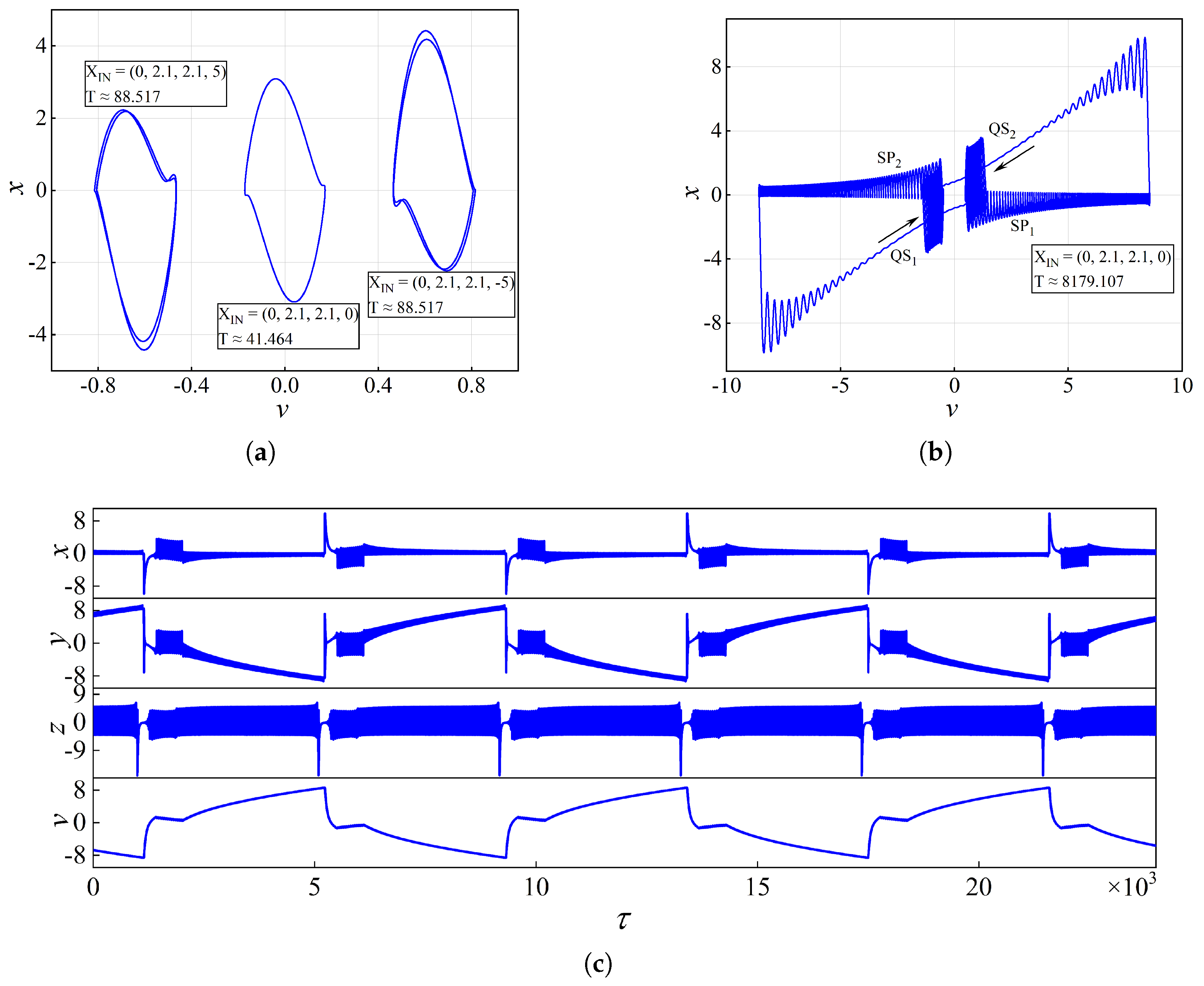
To further illustrate the hidden attractors mentioned above and to provide feasible parameter conditions for exploring the underlying chaotic saddle dynamics, we fix $\alpha =0.02$, $\beta =0.02$, and $\delta =0.4$ and examine two values of $\mu$. At $\mu =0.25$, three coexisting hidden limit cycles emerge (Figure 1a), confirming that hidden multistability can be observed in system (2). At $\mu =0.6$, as shown in Figure 1b,c, the system exhibits a hidden bursting oscillation with two quiescent and two spiking states. During this bursting, v exhibits a periodic relaxation, modulating x, y, and z to alternate between quiescent and spiking states. This reveals a clear slow–fast separation: x, y, and z act as fast variables, while v serves as the slow variable. Particularly, as emphasized by the black boxes in Figure 1b, the relatively large-amplitude oscillations in the spiking states are caused by chaotic saddle dynamics rather than by attractors, which will be investigated in Section 4.

3. Dynamical Analysis of the Fast and Slow Subsystems

The hidden bursting shown in Figure 1b suggests that the full-system state variables can be divided into a fast-variable group $(x,y,z)$ and a single slow variable v, giving rise to a clear slow–fast timescale separation. To quantify this separation, we introduce the small parameter $ϵ=\beta$ explicitly and rewrite system (2) in the standard singularly perturbed form

$$\left\{\begin{array}{c}\dot{x}=y-x+v,\hfill \\ \dot{y}=-\alpha \left(10xz+x^3\right),\hfill \\ \dot{z}=\mu xy-\delta ,\hfill \\ \dot{v}=-ϵx,\hfill \end{array}\right.$$

(4)

where $ϵ=\beta$ measures the ratio between the fast and slow timescales. In the singular limit $ϵ\to 0$, system (4) reduces to the layer problem (fast subsystem), and as such,

$$\left\{\begin{array}{c}\dot{x}=y-x+v,\hfill \\ \dot{y}=-\alpha \left(10xz+x^3\right),\hfill \\ \dot{z}=\mu xy-\delta ,\hfill \end{array}\right.$$

(5)

in which the slow variable v acts as a constant parameter, and the slow problem (slow subsystem) is defined as

$${\displaystyle \frac{dv}{d\tau }}=-ϵx,\mathrm{or}\mathrm{equivalently}{\displaystyle \frac{dv}{dt}}=-x,t=ϵ\tau ,$$

(6)

which describes the slow drift of v on the critical manifold. The layer problem (5) governs the fast dynamics at a fixed v, while the slow problem (6) determines how v evolves along the critical manifold. This decomposition provides the mathematical basis for the slow–fast analysis in the following subsections. For the parameter set used in this paper ($\alpha =0.02$, $\beta =0.02$, $\mu =0.6$, $\delta =0.4$), we have $ϵ=0.02$, which is sufficiently small to justify the separation of timescales observed in Figure 1.

Under this parameter set, the layer problem (5) takes the explicit form

$$\left\{\begin{array}{c}\dot{x}=y-x+v,\hfill \\ \dot{y}=-0.2xz-0.02x^3,\hfill \\ \dot{z}=0.6xy-0.4,\hfill \end{array}\right.$$

(7)

and the slow problem (6) reduces to

$$\dot{v}=-0.02x,$$

(8)

where the numerical coefficients follow from the parameter set corresponding to the hidden bursting in Figure 1b.

In classical bursting dynamics, the quiescent states are typically traced to stable equilibrium sets in the fast subsystem, while the spiking states are traced to stable non-equilibrium sets. The slow variable evolves on a much slower timescale and modulates the fast subsystem as a slowly varying parameter, thereby driving the full-system trajectory through transitions between these distinct dynamical regimes via related bifurcations. In what follows, we analyze the fast subsystem (7) in detail by treating v as a bifurcation parameter, and then examine the dynamics of the slow subsystem (8).

3.1. Equilibrium Analysis of the Fast Subsystem

Treating v as a bifurcation parameter, we first identify the equilibrium points of the fast subsystem (7). Setting $\dot{x}=\dot{y}=\dot{z}=0$ yields two equilibrium branches

$${\mathrm{EB}}_{\pm }:=\left\{(\overline{x},\overline{y},\overline{z})|\overline{x}=x_{\pm }^{*},\overline{y}={\displaystyle \frac{2}{3x_{\pm }^{*}}},\overline{z}=-{\displaystyle \frac{{\left(x_{\pm }^{*}\right)}^2}{10}},x_{\pm }^{*}={\displaystyle \frac{3v\pm \sqrt{9v^2+24}}{6}}\right\},$$

(9)

which together form the critical manifold. The two branches are symmetric about the origin and exist for all $v\in \mathbb{R}$.

The Jacobian evaluated on ${\mathrm{EB}}_{\pm }$ yields the characteristic polynomial

$$f\left(\lambda \right)={\lambda }^3+{\lambda }^2+a_1\lambda +a_2,a_1={\displaystyle \frac{4}{25}}{\overline{x}}^2,a_2={\displaystyle \frac{1}{25}}(3{\overline{x}}^2+2).$$

(10)

Since $a_1>0$ and $a_2>0$ for all $\overline{x}$, the Routh–Hurwitz criterion reduces to $a_1>a_2$, which is equivalent to ${\overline{x}}^2>2$. Under this condition, the corresponding segment of the critical manifold is locally stable. The full-system trajectory restricted to this stable segment corresponds to the quiescent state of the bursting oscillation.

To determine the possible bifurcations on the critical manifold, we compute the discriminant of $f\left(\lambda \right)$, as follows:

$$\Delta =-{\displaystyle \frac{256}{15625}}{\overline{x}}^6-{\displaystyle \frac{11}{625}}{\overline{x}}^4-{\displaystyle \frac{96}{125}}{\overline{x}}^2-{\displaystyle \frac{308}{625}}.$$

(11)

All terms in $\Delta$ are negative for any real $\overline{x}$, hence $\Delta <0$ identically. The characteristic polynomial therefore always possesses one real root and one pair of complex conjugate roots. Since $a_2>0$ rules out fold bifurcations, the only possible bifurcation of equilibria is of the Hopf type.

The Hopf bifurcation condition ${\overline{x}}^2=2$ corresponds to $v=\pm 2\sqrt{2}/3$. At these points, the eigenvalues are ${\lambda }_1=-1$ and ${\lambda }_{2,3}=\pm \frac{2\sqrt{2}}{5}\mathrm{i}$, and the transversality condition $\frac{d\mathrm{Re}\left(\lambda \right)}{dv}{|}_{v=2\sqrt{2}/3}=-\frac{\sqrt{2}}{44}\ne 0$ is satisfied. Furthermore, the non-degeneracy condition is verified numerically, confirming that both Hopf bifurcations are subcritical, as will be shown by numerical continuation in Section 3.3.

At the subcritical Hopf bifurcation, the critical manifold changes from a stable focus to a saddle focus. When the full-system trajectory slides along the stable segment of the critical manifold, it exhibits its quiescent state. As the trajectory drifts past the Hopf point, it is repelled from the now-unstable manifold and exits the quiescent state. The spiking state that follows emerges when the full-system trajectory oscillates along a stable non-equilibrium set, such as a stable limit cycle or a chaotic attractor. For convenience, we term these stable non-equilibrium sets as spike attractors (SPAs). However, for the hidden bursting oscillations considered in this paper, the underlying dynamical mechanisms rely not only on the stable invariant sets of the fast subsystem (7) but also on the unstable invariant sets and their associated bifurcations. Therefore, we will systematically analyze the invariant sets and their dynamics in the next three subsections.

3.2. Invariant Set Structure of the Fast Subsystem at $v=0$

At $v=0$, which lies between the two Hopf bifurcation points identified in Section 3.1, both equilibrium branches ${\mathrm{EB}}_{\pm }$ are saddle foci. The dynamics of the fast subsystem are therefore governed entirely by non-equilibrium invariant sets. Moreover, the fast subsystem possesses the symmetry $(x,y,z)\mapsto (-x,-y,z)$. This makes $v=0$ a natural starting point for examining the invariant sets of the fast subsystem before tracing its evolution under varying v.

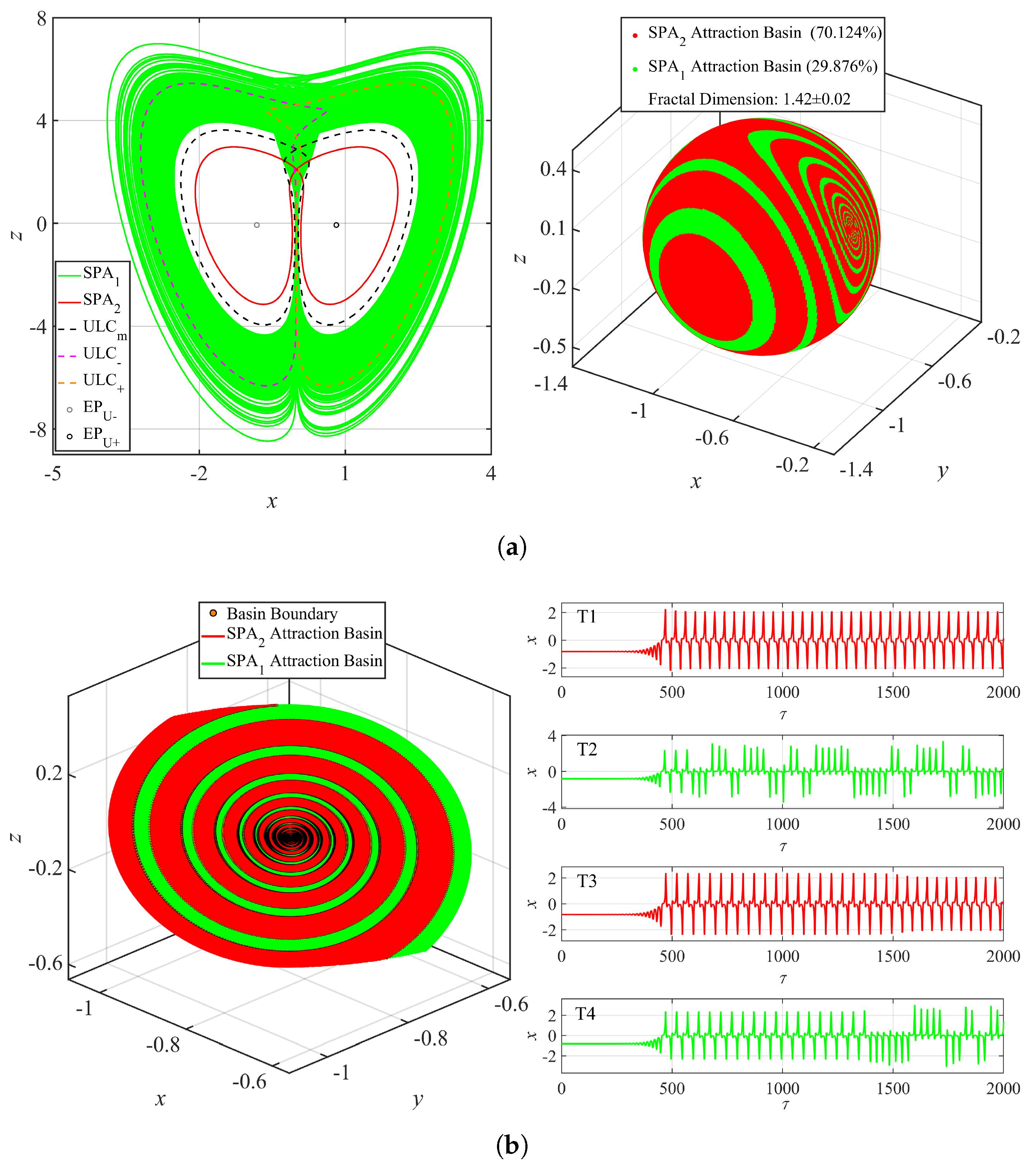
Figure 2a displays the invariant sets (left panel) and the spherical basin portrait (right panel) at $v=0$. The innermost elements are the two saddle foci ${\mathrm{EP}}_{\mathrm{U}\pm }$, enclosed by a stable limit cycle ${\mathrm{SPA}}_2$ (solid red, initialized from $(x,y,z)=(0.1,-0.1,-0.17)$). Surrounding ${\mathrm{SPA}}_2$ lies an unstable limit cycle ${\mathrm{ULC}}_{\mathrm{m}}$ (dashed black). The outermost region contains a chaotic attractor ${\mathrm{SPA}}_1$ (solid green, initialized from $(x,y,z)=(3.1,-3.1,-3.17)$), within which two mutually symmetric unstable limit cycles ${\mathrm{ULC}}_{\pm }$ (dashed orange and magenta) are embedded. The stability indicators of all invariant sets are provided in

Table A1. Summary of the invariant sets in Figure 2a, including stability indicators, values and types.

Invariant Set	Stability Indicator	Value	Type
${\mathrm{SPA}}_1$	Lyapunov exponents $(L{E}_1^{FS},L{E}_2^{FS},L{E}_3^{FS})$	$L{E}_1^{FS}\approx 0.0279$	chaotic attractor
		$L{E}_2^{FS}\approx 0$
		$L{E}_3^{FS}\approx -1.0279$
${\mathrm{SPA}}_2$	Floquet multipliers $({\Lambda }_1^2,{\Lambda }_2^2,{\Lambda }_3^2)$	${\Lambda }_1^2\approx 0.0869$	stable limit cycle
		${\Lambda }_2^2=1$
		${\Lambda }_3^2\approx {10}^{-16}$
${\mathrm{ULC}}_{\mathrm{m}}$	Floquet multipliers $({\Lambda }_1^m,{\Lambda }_2^m,{\Lambda }_3^m)$	${\Lambda }_1^m\approx 3.4612$	saddle limit cycle
		${\Lambda }_2^m=1$
		${\Lambda }_3^m\approx {10}^{-15}$
${\mathrm{ULC}}_{\pm }$	Floquet multipliers $({\Lambda }_1^{\pm },{\Lambda }_2^{\pm },{\Lambda }_3^{\pm })$	${\Lambda }_1^{\pm }\approx 11.0175$	saddle limit cycle
		${\Lambda }_2^{\pm }=1$
		${\Lambda }_3^{\pm }\approx {10}^{-18}$
${\mathrm{EP}}_{\mathrm{U}\pm }$	Eigenvalues $({\lambda }_1^{\pm },{\lambda }_2^{\pm },{\lambda }_3^{\pm })$	${\lambda }_1^{\pm }\approx -1.0045$	saddle focus
		${\lambda }_2^{\pm }\approx 0.0223+0.3907i$
		${\lambda }_3^{\pm }\approx 0.0223-0.3907i$

. Among these sets, ${\mathrm{SPA}}_1$ and ${\mathrm{SPA}}_2$ are both attracting, giving rise to bistability. The spherical basin portrait, computed with a sphere centered at ${\mathrm{EP}}_{\mathrm{U}-}$ (radius $0.5$), shows that their basins occupy approximately $29.876\%$ and $70.124\%$ of the sphere, respectively. The basin boundary is fractal, with an estimated fractal dimension $D_0=1.42\pm 0.02$. The details of the estimation method and the convergence test are provided in Appendix B.

As is well known, the transitions from quiescent to spiking states occur after the critical manifold loses its stability. This means that here, these transitions occur at saddle foci, where the full-system trajectories depart the critical manifold along the unstable manifolds of the saddle foci. This motivates us to explore the transient dynamics of the fast-subsystem trajectories originating from the unstable manifold of ${\mathrm{EP}}_{\mathrm{U}-}$. This can provide us a guideline for understanding hidden bursting in this paper.

We now further investigate this through basin analysis in the region near the unstable manifold of ${\mathrm{EP}}_{\mathrm{U}-}$, as shown in Figure 2b. The left panel shows the basins in this region, and the right panel shows four representative trajectories (T1–T4). Trajectories deep within distinct basins converge rapidly to their respective attractors (T1 to ${\mathrm{SPA}}_2$, T2 to ${\mathrm{SPA}}_1$). Along the basin boundary, a heteroclinic connection links ${\mathrm{EP}}_{\mathrm{U}-}$ to the saddle limit cycle ${\mathrm{ULC}}_{\mathrm{m}}$. From ${\mathrm{ULC}}_{\mathrm{m}}$, two distinct routes emerge: T3 approaches ${\mathrm{SPA}}_2$, while T4 converges to ${\mathrm{SPA}}_1$. This identifies ${\mathrm{ULC}}_{\mathrm{m}}$ as a gateway. Here and throughout this paper, a gateway refers to a saddle-type invariant set whose stable and unstable manifolds mediate the transition between two coexisting attractors, so that trajectories on the basin boundary pass through a neighborhood of this set before converging to either attractor. Assuming that the full system (2) exits a quiescent state near ${\mathrm{EP}}_{\mathrm{U}-}$ at $v=0$, the following spiking state can be predicted by the four representative trajectories (T1–T4) shown in Figure 2b.

In summary, at $v=0$, the fast subsystem possesses a layered invariant set structure with ${\mathrm{ULC}}_{\mathrm{m}}$ acting as the basin boundary between the chaotic attractor ${\mathrm{SPA}}_1$ and the stable limit cycle ${\mathrm{SPA}}_2$. This structure serves as the reference configuration for the numerical continuation analysis presented in the next subsection.

3.3. Bifurcation Analysis via Numerical Continuation

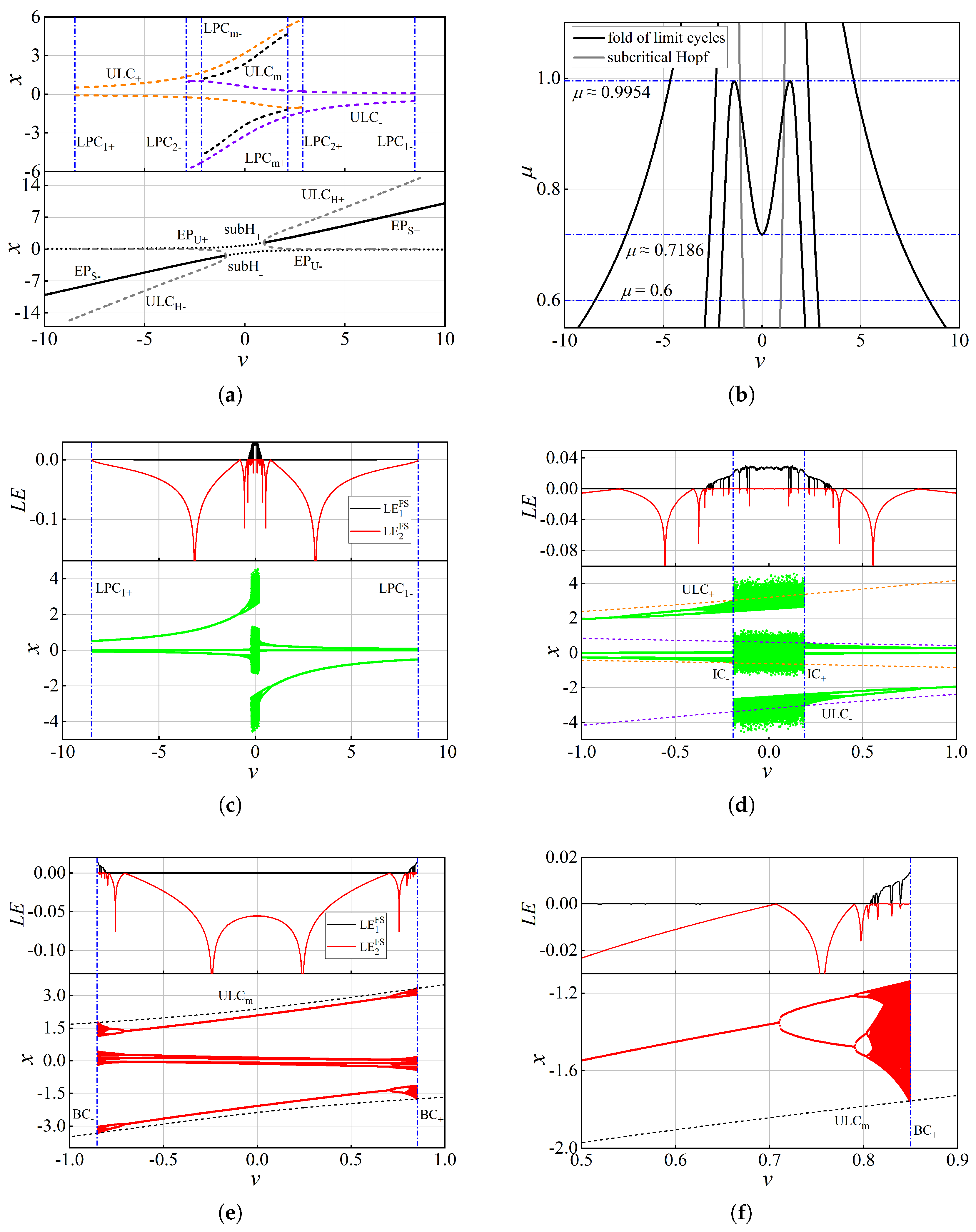
Building on the structure at $v=0$, we now treat v as a continuously varying parameter to track the evolution of these invariant sets and their bifurcations via numerical continuation. Figure 3 shows the resulting bifurcation diagrams for $v\in [-10,10]$. The key bifurcation points detected during continuation are listed in

Table A2. Key bifurcations in Figure 3, including labels, types and critical values.

Bifurcation Label	Bifurcation Type	Critical Value
${\mathrm{IC}}_{\pm }$	interior crisis	$v\approx \pm 0.1859$
${\mathrm{BC}}_{\pm }$	boundary crisis	$v\approx \pm 0.8492$
${\mathrm{subH}}_{\pm }$	subcritical Hopf	$v\approx \pm 0.9428$
${\mathrm{LPC}}_{\mathrm{m}\pm }$	fold of limit cycles	$v\approx \pm 2.1165$
${\mathrm{LPC}}_{2\pm }$	fold of limit cycles	$v\approx \pm 2.8282$
${\mathrm{LPC}}_{1\pm }$	fold of limit cycles	$v\approx \mp 8.4609$

.

In Figure 3a, two subcritical Hopf bifurcations ${\mathrm{subH}}_{\pm }$ divide the equilibrium branches ${\mathrm{EB}}_{\pm }$ into stable foci ${\mathrm{EB}}_{\mathrm{S}\pm }$ (solid black) and saddle foci ${\mathrm{EB}}_{\mathrm{U}\pm }$ (dotted black). Unstable limit cycles ${\mathrm{ULC}}_{\mathrm{H}\pm }$ (dashed gray) emanate from these Hopf points, each surrounding the corresponding stable focus branch. The three unstable limit cycles vanish via the folds of limit cycles: ${\mathrm{ULC}}_{\mathrm{m}}$ at ${\mathrm{LPC}}_{\mathrm{m}\pm }$ and ${\mathrm{ULC}}_{\pm }$ at ${\mathrm{LPC}}_{2\pm }$.

By continuing the bifurcation points obtained from Figure 3a in two parameters using MatCont [38], we can plot the two-parameter bifurcation sets in the $(v,\mu )$-plane (Figure 3b) with $\mu \in [0.55,1.1]$. Within the focused area, although the subcritical Hopf bifurcation set (gray curves) monotonically extends with increasing $\mu$, two critical values, $\mu \approx 0.7186$ and $\mu \approx 0.9954$, divide the fold of limit cycles bifurcation set (black curves) into three regions. These three regions correspond to three bifurcation regimes where v continuously varies from $-10$ to 10. Specifically, we can detect six, eight and four folds of limit cycles in $\mu \in (0.55,0.7186)$, $\mu \in (0.7186,0.9954)$ and $\mu \in (0.9954,1.1)$, respectively.

Figure 3c,e display the one-parameter bifurcation analyses for the attractors ${\mathrm{SPA}}_1$ and ${\mathrm{SPA}}_2$, assisted with the computed Lyapunov exponents, showing that these two attractors undergo more intricate transitions. Specifically, ${\mathrm{SPA}}_1$ collides with the saddle limit cycles ${\mathrm{ULC}}_{\pm }$ at $v\approx \pm 0.1859$, after which the chaotic attractor is confined to the region enclosed by these two unstable limit cycles. This event marks two interior crises ${\mathrm{IC}}_{\pm }$ (Figure 3d). Following these crises, ${\mathrm{SPA}}_1$ undergoes an inverse period-doubling cascade and becomes a stable limit cycle, which persists until $v\approx \mp 8.4609$, where it vanishes via a fold of limit cycles, denoted ${\mathrm{LPC}}_{1\pm }$. Meanwhile, ${\mathrm{SPA}}_2$ undergoes a period-doubling cascade to chaos. Its subsequent collision with the middle unstable limit cycle ${\mathrm{ULC}}_{\mathrm{m}}$ at $v\approx \pm 0.8492$ induces boundary crises ${\mathrm{BC}}_{\pm }$ (Figure 3e,f), after which ${\mathrm{SPA}}_2$ ceases to exist.

It is well established that interior and boundary crises induce transient chaos, with chaotic saddles typically accompanied by narrow periodic windows that vanish rapidly as the parameter varies [39,40,41]. This implies that the chaotic saddle dynamics induced by the crises ${\mathrm{IC}}_{\pm }$ and ${\mathrm{BC}}_{\pm }$ govern the fast subsystem, a key mechanism for the hidden bursting studied here. However, chaotic saddles are inherently difficult to visualize. Alternatively, we can trace the representative low-period unstable limit cycles, whose intertwined manifolds form the fundamental skeleton of the chaotic saddle [39].

Here and throughout this paper, the skeleton of a chaotic saddle refers to the collection of low-period unstable limit cycles whose intertwined stable and unstable manifolds form the fundamental geometric structure of the chaotic saddle, and among which trajectories on the chaotic saddle wander. Thus, in the next subsection, we investigate these fast-subsystem dynamics by tracking these cycles and their bifurcations.

3.4. Chaotic Saddle Dynamics in the Fast Subsystem

Following the premise introduced above, we characterize the chaotic saddle dynamics by tracing the evolution of representative unstable limit cycles as v varies, combined with a verification of transient chaos. Owing to the system’s symmetry, we focus on the chaotic saddle labeled ${\mathrm{CS}}_{+}$, located within the parameter regime $v>0$.

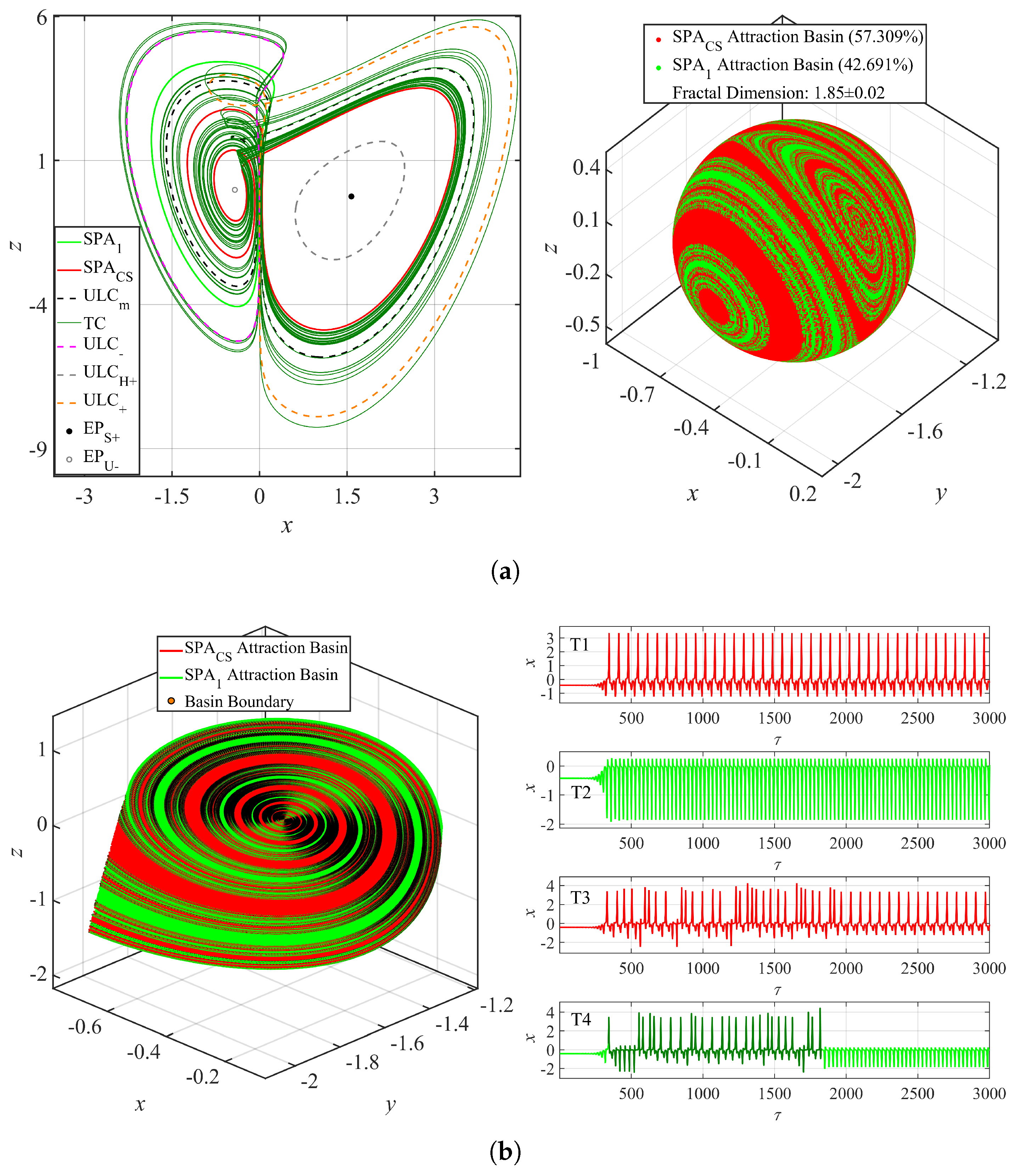
After the crises ${\mathrm{IC}}_{+}$ and ${\mathrm{BC}}_{+}$, as v increases, we employ the four low-period unstable limit cycles ${\mathrm{ULC}}_{\mathrm{m}}$, ${\mathrm{ULC}}_{+}$, ${\mathrm{ULC}}_{-}$, and ${\mathrm{ULC}}_{\mathrm{H}+}$ (shown in Figure 3a) to probe the chaotic saddle dynamics in the fast subsystem. We first examine the fast subsystem at $v=1.15$, where an additional stable limit cycle ${\mathrm{SPA}}_{\mathrm{CS}}$ emerges, initialized from $(x,y,z)=(-1,1.5,-2)$. This introduces a tristable regime among ${\mathrm{SPA}}_{\mathrm{CS}}$, ${\mathrm{SPA}}_1$, and the stable focus ${\mathrm{EP}}_{\mathrm{S}+}$. To further explore the underlying chaotic saddle dynamics, Figure 4 presents a detailed dynamical analysis at this parameter point.

The left panel of Figure 4a shows the observed invariant sets. The transient chaotic trajectory $\mathrm{TC}$ (dark green), extracted from trajectory T4 in Figure 4b, traces a structure that approximates the chaotic saddle ${\mathrm{CS}}_{+}$, with ${\mathrm{SPA}}_{\mathrm{CS}}$ lying close to its edge. This trajectory wanders among the three unstable limit cycles ${\mathrm{ULC}}_{\pm }$ and ${\mathrm{ULC}}_{\mathrm{m}}$, indicating that these cycles act as the fundamental skeleton of ${\mathrm{CS}}_{+}$.

The spherical basin portrait (right panel of Figure 4a) reveals that ${\mathrm{SPA}}_{\mathrm{CS}}$ and ${\mathrm{SPA}}_1$ occupy approximately $57.309\%$ and $42.691\%$ of the sphere, respectively. The basin of ${\mathrm{EP}}_{\mathrm{S}+}$ is absent from the portrait because, for the chosen sphere radius, this attractor has no basin points on the spherical surface. Unlike the smooth spiral patterns observed at $v=0$, the basin boundary here is highly fragmented, with a fractal dimension $D_0=1.85\pm 0.02$, which is significantly higher than $D_0=1.42\pm 0.02$ at $v=0$. This suggests that the unstable manifold of ${\mathrm{EP}}_{\mathrm{U}-}$ connects to the stable manifold of ${\mathrm{CS}}_{+}$.

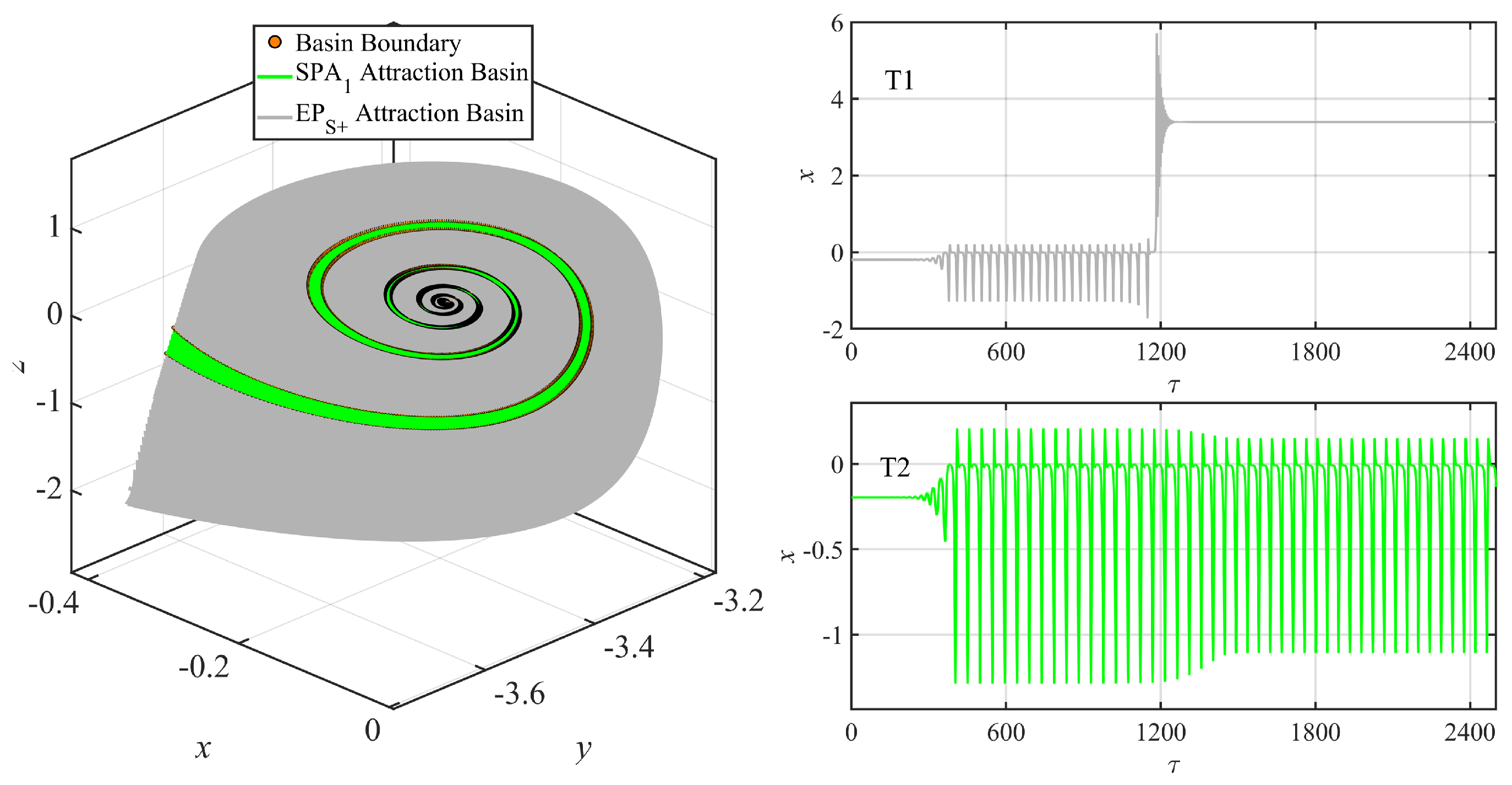
The basin structure near the unstable manifold of ${\mathrm{EP}}_{\mathrm{U}-}$ (left panel of Figure 4b) reveals a far more complex basin boundary than that at $v=0$. This complexity can be further illustrated by the four representative trajectories in the right panel of Figure 4b. Trajectories deep within individual basins (T1, T2) converge rapidly. Near the basin boundaries, T3 and T4 first enter the region of the chaotic saddle, exhibiting prolonged transient chaos before converging to their respective attractors. Each basin boundary therefore defines a heteroclinic connection from ${\mathrm{EP}}_{\mathrm{U}-}$ to ${\mathrm{CS}}_{+}$, and ${\mathrm{CS}}_{+}$ serves as the gateway mediating transitions between ${\mathrm{SPA}}_1$ and ${\mathrm{SPA}}_{\mathrm{CS}}$.

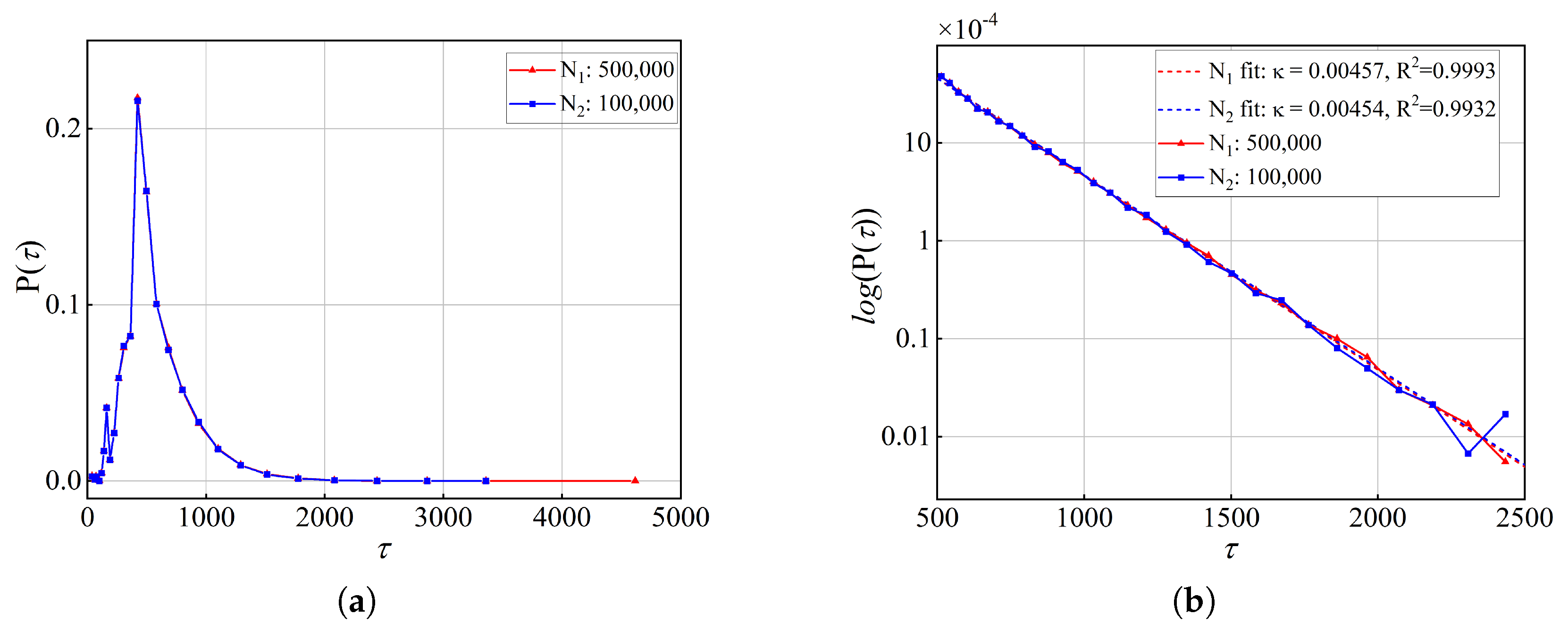
To provide direct evidence for the chaotic saddle that organizes the basin structure, we perform spherical sprinkling on a sphere of radius $r=0.15$ centered at the maximum point of the saddle-type limit cycle ${\mathrm{ULC}}_m$. This center is chosen for two reasons. First, since ${\mathrm{ULC}}_m$ forms part of the skeleton of the chaotic saddle ${\mathrm{CS}}_{+}$, placing the center at its maximum ensures that the sphere intersects ${\mathrm{CS}}_{+}$ transversely. Second, the radius $r=0.15$ is chosen, as it is small enough that the sphere does not intersect any coexisting attractor, so that the sprinkled initial conditions probe the transient region rather than converging immediately to an attractor. Initial conditions are distributed quasi-uniformly on the sphere using Fibonacci sampling, and each is integrated with an adaptive Runge–Kutta–Fehlberg (RK45) scheme (tolerances ${10}^{-8}$) until it reaches an $\epsilon$-neighborhood ($\epsilon ={10}^{-3}$) of either ${\mathrm{SPA}}_1$ or ${\mathrm{SPA}}_{CS}$. To verify convergence, we use $N=\mathrm{100,000}$ and $N=\mathrm{500,000}$ initial conditions. The escape-time distributions $P\left(\tau \right)$ are shown in Figure 5a. Both curves exhibit a well-defined exponential regime over $\tau \in [500,2500]$, spanning nearly five orders of magnitude. Least-squares fits of $logP\left(\tau \right)$ versus $\tau$ over the exponential regime (Figure 5b) give $\kappa =0.00454\pm 0.00013$ ($N=\mathrm{100,000}$) and $\kappa =0.00457\pm 0.00007$ ($N=\mathrm{500,000}$), where the uncertainties are 95% confidence intervals from the linear regression. The two values agree within $0.63\%$, confirming convergence of the transient lifetime statistics. The coefficients of determination are $R^2=0.9932$ and $R^2=0.9993$, respectively, confirming the exponential character of the distribution.

Collectively, these observations establish a causal link among the chaotic saddle, the fractal basin boundaries, and the prolonged transient chaos: the existence of ${\mathrm{CS}}_{+}$ manifests itself through the highly fragmented basins and the heteroclinic connections from ${\mathrm{EP}}_{\mathrm{U}-}$ to ${\mathrm{CS}}_{+}$. In contrast, once the saddle’s skeleton collapses, we expect these fractal boundaries and long-lived chaotic transients to vanish simultaneously. The analysis at $v=3.2$ below confirms this prediction and serves as a direct indicator for the disappearance of ${\mathrm{CS}}_{+}$.

Although ${\mathrm{ULC}}_{\mathrm{m}}$ forms part of the skeleton supporting the chaotic saddle ${\mathrm{CS}}_{+}$, its disappearance via ${\mathrm{LPC}}_{\mathrm{m}+}$ does not immediately destroy the saddle. Instead, the unstable limit cycle ${\mathrm{ULC}}_{\mathrm{H}+}$, which originates from ${\mathrm{subH}}_{+}$, joins ${\mathrm{ULC}}_{\pm }$ to form a new skeleton that sustains the chaotic saddle. Moreover, a heteroclinic orbit from ${\mathrm{EP}}_{\mathrm{U}-}$ to ${\mathrm{ULC}}_{\mathrm{H}+}$ emerges at $v\approx 2.1432$, thereby mediating a transition route ${\mathrm{EP}}_{\mathrm{U}-}\to {\mathrm{ULC}}_{\mathrm{H}+}\to {\mathrm{EP}}_{\mathrm{S}+}$. This reconstructed skeleton persists until ${\mathrm{ULC}}_{+}$ disappears via ${\mathrm{LPC}}_{2+}$, at which point the supporting structure is destroyed and the chaotic saddle collapses rapidly.

Considering that the chaotic saddle dynamics within the parameter regime $v>2$ do not participate in the hidden bursting studied in this paper, we select a value of v exceeding ${\mathrm{LPC}}_{2+}$ to investigate the dissolution of ${\mathrm{CS}}_{+}$.

For example, at $v=3.2$, where the parameter exceeds ${\mathrm{LPC}}_{2+}$ ($v\approx 2.8282$) but is not too far from it, the fast subsystem exhibits a bistable regime between ${\mathrm{EP}}_{\mathrm{S}+}$ and ${\mathrm{SPA}}_1$. Figure 6 displays the dynamical analysis near ${\mathrm{EP}}_{\mathrm{U}-}$ at this parameter point. In the basin portrait (left), two accompanying spiral-shaped basin boundaries divide the region near ${\mathrm{EP}}_{\mathrm{U}-}$ into two parts. This is similar to the case at $v=0$ but entirely different from that at $v=1.15$, indicating that ${\mathrm{CS}}_{+}$ has disappeared. Meanwhile, the two representative trajectories (T1 and T2) show that each basin boundary defines a heteroclinic connection from ${\mathrm{EP}}_{\mathrm{U}-}$ to ${\mathrm{ULC}}_{\mathrm{H}+}$, with ${\mathrm{ULC}}_{\mathrm{H}+}$ serving as the gateway mediating transitions between ${\mathrm{SPA}}_1$ and ${\mathrm{EP}}_{\mathrm{S}+}$.

According to the above analysis, as v increases, the chaotic saddle ${\mathrm{CS}}_{+}$ emerges via the interior crisis ${\mathrm{IC}}_{+}$ and subsequently collapses following the fold of limit cycles ${\mathrm{LPC}}_{2+}$. Thus, considering the symmetry, we identify two mutually symmetric chaotic saddles, ${\mathrm{CS}}_{+}$ and ${\mathrm{CS}}_{-}$, which exist in the ranges $v\in [{\mathrm{IC}}_{+},{\mathrm{LPC}}_{2+}]$ and $v\in [{\mathrm{LPC}}_{2-},{\mathrm{IC}}_{-}]$, respectively. Here and throughout this paper, a chaotic saddle range refers to the interval of the slow variable v over which the corresponding chaotic saddle ${\mathrm{CS}}_{\pm }$ exists in the fast subsystem; it is bounded below by the interior crisis ${\mathrm{IC}}_{\pm }$ and above by the fold of limit cycles ${\mathrm{LPC}}_{2\pm }$ (see Table A2).

Notably, within these ranges, the two chaotic saddles coexist with a persistent spike attractor ${\mathrm{SPA}}_1$. As will be shown, whenever a hidden bursting trajectory exits a quiescent state within these ranges, this coexistence gives rise to a subsequent spiking state that is not only diverse but also unpredictable. Moreover, unlike slow–fast systems driven solely by slow external excitation, our slow subsystem (8) features a feedback loop in which v receives input from the fast variable x while simultaneously modulating the fast-subsystem dynamics. This feedback loop further exacerbates the complexity of the hidden bursting dynamics, thus motivating us to investigate the slow-subsystem dynamics in the next subsection.

3.5. Dynamics of the Slow Subsystem

In the slow subsystem (8), the condition $\dot{v}=0$ defines the v-nullcline at $x=0$, from which three distinct evolutionary scenarios emerge:

(i)

Confined trajectory: If the full-system trajectory evolves entirely within the half-plane $x>0$, then $\dot{v}<0$ and v decreases monotonically. Conversely, if the trajectory remains within $x<0$, then $\dot{v}>0$ and v increases monotonically.

(ii)

Nullcline crossing: If the trajectory crosses $x=0$, the sign of $\dot{v}$ reverses, and the drift direction of v changes accordingly.

(iii)

Needle-threading behavior: If the trajectory repeatedly pierces the nullcline $x=0$, the drift direction of v reverses periodically, generating sustained oscillations of the slow variable.

Here and throughout this paper, the term needle-threading behavior refers to the scenario in (iii), i.e., the repeated crossing of the v-nullcline $x=0$ by a trajectory, which periodically reverses the drift direction of the slow variable v and thereby sustains the slow oscillations.

For a needle-threading trajectory $\Gamma (x_i,y_i,z_i,v_i)$ with $i=1,2,\dots ,n$, we define the arithmetic mean of the x-coordinate as

$$X_{\mathrm{AVER}}={\displaystyle \frac{1}{n}}{\displaystyle \sum _{i=1}^n}{x}_i.$$

(12)

When $X_{\mathrm{AVER}}>0$, the slow variable v drifts toward the negative direction over the duration of the sustained oscillations. Conversely, when $X_{\mathrm{AVER}}<0$, the drift direction is toward a positive v. In the special case $X_{\mathrm{AVER}}\approx 0$, the net change in v between the endpoints of $\Gamma$ is negligible.

The dynamics of v can therefore be understood through the attractors that govern the fast subsystem at a given v. For instance, the two equilibrium branches ${\mathrm{EB}}_{\pm }$ are confined to the half-planes $x>0$ and $x<0$, respectively, implying that v evolves monotonically when the full-system trajectory slides along either branch.

In addition, as shown in Figure 3c,e, the two attractors ${\mathrm{SPA}}_1$ and ${\mathrm{SPA}}_2$ straddle the v-nullcline within their ranges of existence. Taking ${\mathrm{SPA}}_1$ at $v=1.15$ as an example (see Figure 4a), it lies predominantly in the region $x<0$. Consequently, one full cycle along ${\mathrm{SPA}}_1$ yields $X_{\mathrm{AVER}}<0$, resulting in a net increase in v. A similar reasoning applies to other attractors and their combinations. We note that the needle-threading behavior is not restricted to attractors. Transient chaotic trajectories, such as those wandering near the chaotic saddle ${\mathrm{CS}}_{+}$, also repeatedly cross the v-nullcline, and their net drift direction is governed by the sign of $X_{\mathrm{AVER}}$ in the same manner. This will be shown to play a crucial role in shaping the transition-path modes during bursting, as discussed in Section 4.

4. Hidden Bursting Oscillations and Generation Mechanisms

Building on the slow–fast decomposition established in Section 3, this section presents a numerical exploration of the hidden bursting phenomena and their generation mechanisms, with particular emphasis on the role of chaotic saddle dynamics.

As illustrated by the basin analysis in Figure 4b, the fast subsystem (7) exhibits high sensitivity to initial conditions near the saddle focus, owing to the presence of the chaotic saddle. This sensitivity implies that the full system is also highly sensitive to the slow adaptation strength $\beta$ whenever the full-system trajectories evolve on the chaotic saddles. A small change in $\beta$ alters the rate at which v evolves, thereby shifting the entry conditions into the chaotic saddle regime. The resulting variation in transition behavior motivates us to study the bursting phenomena using $\beta$ as a control parameter.

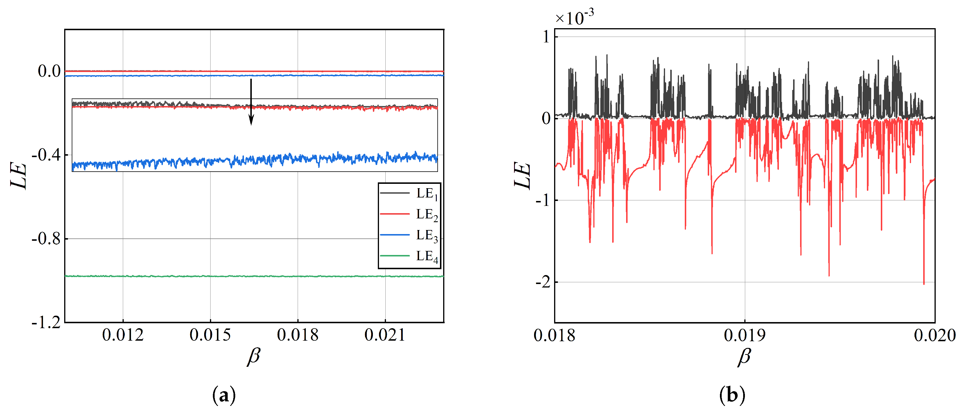
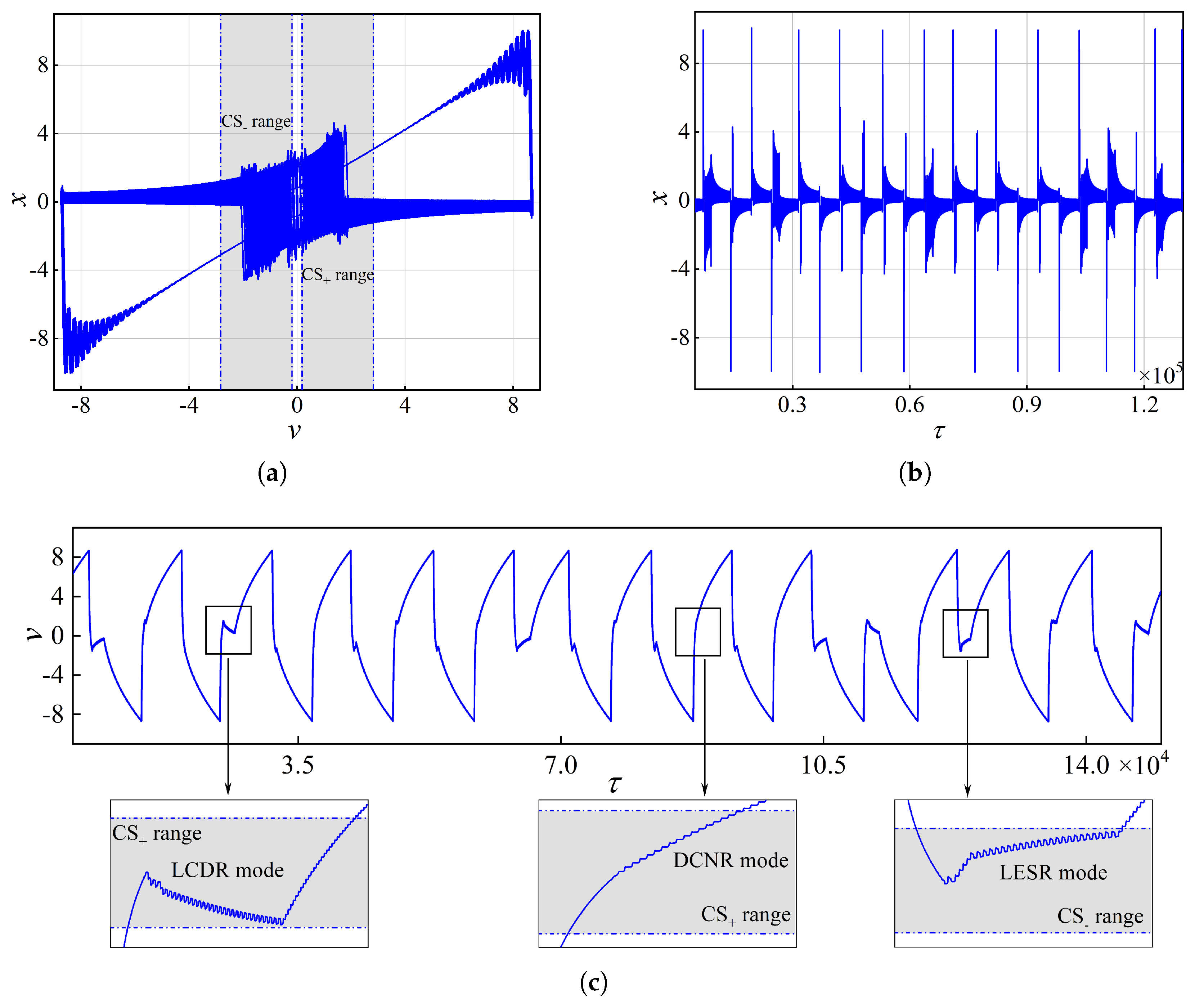
As a preliminary investigation, we compute the Lyapunov exponent spectrum of the full system for $\beta \in [0.01,0.023]$, sorted as $L{E}_1>L{E}_2>L{E}_3>L{E}_4$, as shown in Figure 7a. From a macroscopic viewpoint, the four Lyapunov exponents appear nearly constant over this interval, with the largest exponents on the order of ${10}^{-3}$. However, the magnified view reveals that the exponents actually exhibit small-scale but violent oscillations as $\beta$ varies. This further confirms that the full-system dynamics are highly sensitive to the slow adaptation strength. As shown in Figure 7b, this sensitivity becomes even more pronounced when we focus on the $\beta$ range $[0.018,0.02]$ and isolate the largest and second-largest Lyapunov exponents. Within this narrow window, the full system displays frequent alternations between periodic and chaotic behaviors. Furthermore,

Table A3. Lyapunov exponents of the bursting patterns analyzed in this paper, extracted from Figure 11. Values of order ${10}^{-5}$ or smaller are taken as zero.

Parameter $\mathit{\beta }$	Location (Figure)	$({\mathit{LE}}_1,{\mathit{LE}}_2,{\mathit{LE}}_3,{\mathit{LE}}_4)$
$0.01322$	Figure 12a	$(0.0008,0,-0.0213,-0.9794)$
$0.01826$	Figure 11b	$(0,-0.0007,-0.0201,-0.9792)$
$0.0192$	Figure 11a	$(0,-0.0005,-0.0203,-0.9792)$
$0.01972$	Figure 10a	$(0,-0.0007,-0.0211,-0.9781)$
$0.01984$	Figure 9a	$(0,-0.0009,-0.0192,-0.9799)$
$0.02$	Figure 8a	$(0,-0.0007,-0.0211,-0.9781)$

lists the Lyapunov exponents of the six bursting patterns presented in this paper, extracted from the Lyapunov spectrum in Figure 7. The five periodic bursting patterns are each located within different periodic windows.

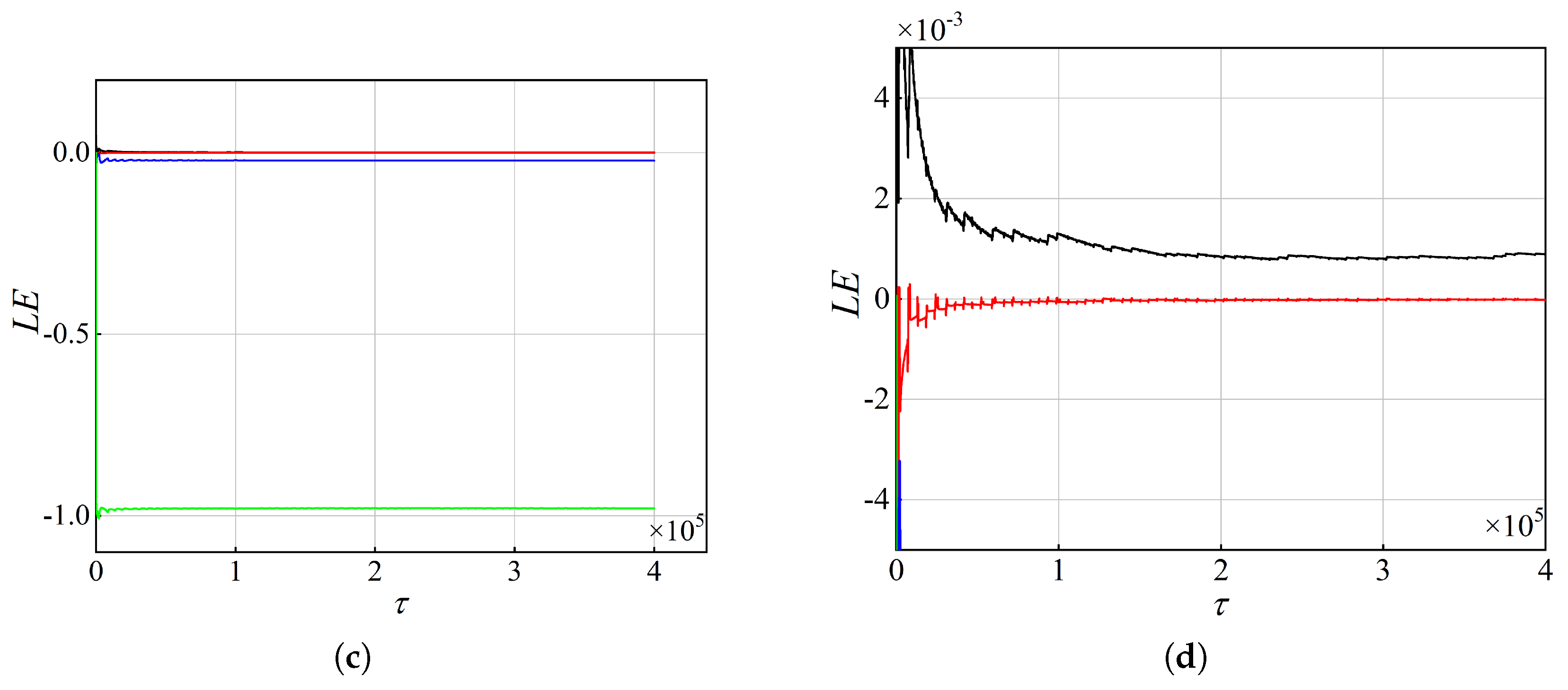
To verify the convergence of the largest Lyapunov exponent, Figure 7c,d show $L{E}_1$ at $\beta =0.01322$ as a function of the integration time $\tau$. The first $5\times {10}^4$ time units are discarded as transient, and the exponent is computed over a total of $4\times {10}^5$ time units. As shown in the local magnification in Figure 7d, $L{E}_1$ converges to a constant positive value of approximately $0.0008$ for $\tau \ge 2\times {10}^5$, confirming that the positive exponent reflects genuine weak chaos rather than a long transient or quasiperiodic dynamics.

4.1. Hidden Delayed-subH/LPC Bursting with Lift-Captured Double-Reversal (LCDR)

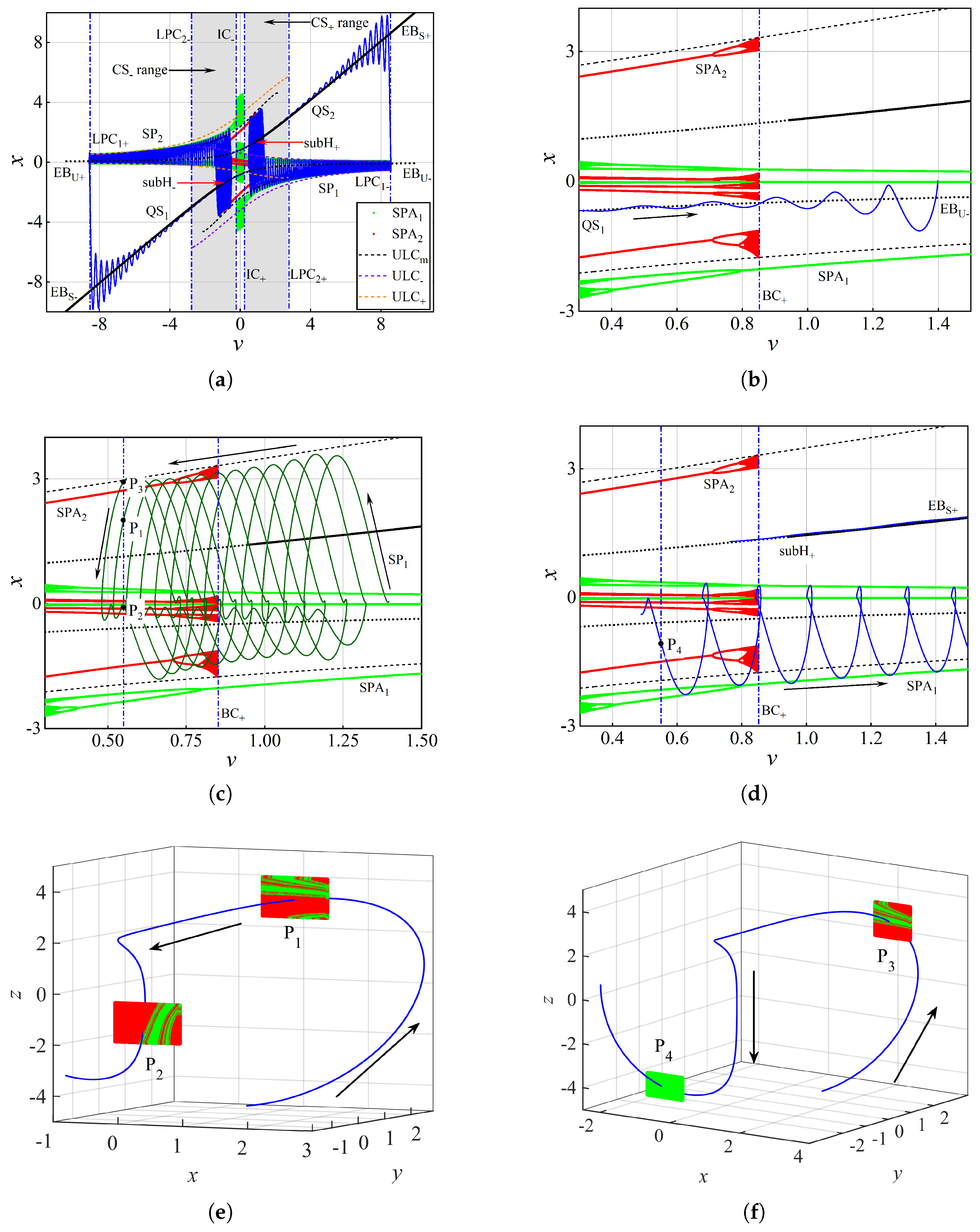
In this subsection, we investigate the dynamical generation mechanism for the periodic bursting phenomenon shown in Figure 1b at $\beta =0.02$. Superimposing the bursting trajectory onto the one-parameter bifurcation diagram, Figure 8a illustrates the general generation mechanism for this bursting pattern via the classical slow–fast analysis method.

Generally speaking, the spiking states ${\mathrm{SP}}_i(i=1,2)$ and the quiescent states ${\mathrm{QS}}_i(i=1,2)$ can be explained by the full-system trajectory evolving on different attractors of the fast subsystem. The quiescent state ${\mathrm{QS}}_1$ is caused by the trajectory sliding along the lower stable equilibrium branch ${\mathrm{EB}}_{\mathrm{S}-}$, while the spiking state ${\mathrm{SP}}_1$ is induced by the trajectory mainly oscillating along the right branch of ${\mathrm{SPA}}_1$. The dynamical causation for ${\mathrm{QS}}_2$ and ${\mathrm{SP}}_2$ follows immediately by symmetry. During this bursting rhythm, two important bifurcations govern the four transitions between spiking and quiescent states. The two subcritical Hopf bifurcations ${\mathrm{subH}}_{\pm }$, which destabilize ${\mathrm{EB}}_{\mathrm{S}\pm }$, dominate the transition routes ${\mathrm{QS}}_1\to {\mathrm{SP}}_1$ and ${\mathrm{QS}}_2\to {\mathrm{SP}}_2$. The two folds of limit cycles ${\mathrm{LPC}}_{1\mp }$, where ${\mathrm{SPA}}_1$ disappears, govern the transition routes ${\mathrm{SP}}_1\to {\mathrm{QS}}_2$ and ${\mathrm{SP}}_2\to {\mathrm{QS}}_1$.

Note that ${\mathrm{subH}}_{-}$ lies within ${\mathrm{CS}}_{-}$ while ${\mathrm{subH}}_{+}$ lies within ${\mathrm{CS}}_{+}$. However, the transition ${\mathrm{QS}}_1\to {\mathrm{SP}}_1$ occurs within ${\mathrm{CS}}_{+}$, and ${\mathrm{QS}}_2\to {\mathrm{SP}}_2$ occurs within ${\mathrm{CS}}_{-}$. Each transition therefore takes place in the chaotic saddle range opposite to that containing the corresponding Hopf bifurcation. Moreover, both spiking states ${\mathrm{SP}}_i(i=1,2)$ exhibit a sudden amplitude change within these chaotic saddle ranges. Together, these features define a unique bursting dynamic structure. To illustrate this, we consider the bursting trajectory that passes near ${\mathrm{subH}}_{-}$ and then remains within the ${\mathrm{CS}}_{+}$ range. For convenience, we divide this unique bursting structure into three stages, sequentially denoted as Stage I (Figure 8b), Stage II (Figure 8c), and Stage III (Figure 8d).

First of all, the slow passage effect, which is a common feature of Hopf bifurcations in slow–fast dynamics [42], appears near ${\mathrm{subH}}_{-}$ within the ${\mathrm{CS}}_{-}$ range. This delays the transition, allowing the full-system trajectory to remain in the quiescent state ${\mathrm{QS}}_1$ until it enters the ${\mathrm{CS}}_{+}$ range. There, the full system gradually departs from the unstable equilibrium branch ${\mathrm{EB}}_{\mathrm{U}-}$, entering Stage I before crossing the v-nullcline at $x=0$. During this stage, the trajectory is confined within the negative x-half-plane. Accordingly, the slow variable v monotonically increases toward the positive-v direction.

After Stage I, the trajectory transitions to ${\mathrm{SP}}_1$ by crossing the v-nullcline at $v\approx 1.4$. Near this v-range, heteroclinic connections from the saddle focus ${\mathrm{EB}}_{\mathrm{U}-}$ to ${\mathrm{CS}}_{+}$, as illustrated in Figure 4, can enhance the dynamical complexity. Here and throughout this paper, lift refers to the process by which a trajectory entering the chaotic saddle range is temporarily trapped by the chaotic saddle and thereby acquires a cluster of large-amplitude oscillations instead of converging directly to a coexisting attractor. For instance, here, the trajectory, lifted by ${\mathrm{CS}}_{+}$, exhibits a cluster of large-amplitude oscillations (dark green curve in Figure 8c). These large-amplitude oscillations, which define Stage II, are analogous to the transient chaotic trajectories wandering around the unstable limit cycle ${\mathrm{ULC}}_{\mathrm{m}}$. As $\tau$ increases, these oscillations also exhibit needle-threading behavior, accompanied by a gradually diminishing positive shift in the x-direction. Here, the needle-threading behavior manifests as oscillations in v, while the positive shift corresponds to a positive arithmetic mean of x, as defined in Equation (12). Quantitatively, the mean over this stage is computed as $X_{\mathrm{AVER}}\approx 0.0719$. Accordingly, v displays biased oscillations with a small net negative change per cycle. This reverses the bursting evolution path toward the negative-v direction, so that the large-amplitude oscillations, modulated by v, extend into the negative-v direction.

At the later stage of the large-amplitude oscillations, the full-system trajectory, still remaining on ${\mathrm{CS}}_{+}$, enters a bistability regime consisting of ${\mathrm{SPA}}_1$ and ${\mathrm{SPA}}_2$. At this moment, it faces a competition between these coexisting attractors. Here and throughout this paper, capture refers to the process in which a trajectory leaving the chaotic saddle converges to one of the coexisting attractors of the fast subsystem, such as ${\mathrm{SPA}}_1$ or ${\mathrm{SPA}}_2$; the outcome of capture is determined by which basin the trajectory enters. To determine the selection outcome, we perform a basin analysis on the last two oscillations. Instead of using the entire trajectory, we sequentially extract four representative points at $v=0.55$, labeled ${\mathrm{P}}_i$ ($i=1,2,3,4$). Figure 8e shows the trajectory approaching the fractal basin boundaries from within the basin of ${\mathrm{SPA}}_2$ during the evolution from ${\mathrm{P}}_1$ to ${\mathrm{P}}_2$. In contrast, Figure 8f shows that the trajectory at ${\mathrm{P}}_3$, located on the fractal basin boundary, enters the basin of ${\mathrm{SPA}}_1$ at ${\mathrm{P}}_4$, a point far from the boundary. This indicates that the trajectory is ultimately captured by ${\mathrm{SPA}}_1$, resulting in an abrupt amplitude decrease in ${\mathrm{SP}}_1$.

Subsequently, the trajectory exhibits needle-threading behavior by repeating the oscillation structure of ${\mathrm{SPA}}_1$, thereby defining Stage III. During this stage, ${\mathrm{SPA}}_1$ is predominantly confined to the $x<0$ half-plane, only briefly piercing into $x>0$. This strong negative bias is confirmed by the calculated mean, $X_{\mathrm{AVER}}\approx -0.2329$, whose magnitude is more than three times that of Stage II. This large negative $X_{\mathrm{AVER}}$ imparts a strong net positive increment per cycle in v. Consequently, v exhibits a staircase-like pattern in the positive-v direction. This reverses the bursting evolution path again, regulating ${\mathrm{SP}}_1$ toward the positive-v direction along ${\mathrm{SPA}}_1$.

So far, via slow–fast decomposition, we have revealed the generation mechanism underlying the symmetric periodic delayed-subH/LPC bursting at $\beta =0.02$. This bursting is characterized by a lift-captured double-reversal induced by chaotic saddle dynamics. To highlight the organizing role of the chaotic saddle, and to distinguish it from the classical delayed-subH/LPC bursting paradigm, we denote this bursting pattern as the hidden delayed-subH/LPC bursting with lift-captured double-reversal (LCDR). In the following subsections, this classification scheme will be consistently applied to identify other types of hidden bursting.

4.2. Hidden Delayed-subH/LPC Bursting with Lift-Escape Single-Reversal (LESR)

A slight reduction in the slow adaptation strength from $\beta =0.02$ to $\beta =0.01984$ qualitatively changes the bursting pattern. At $\beta =0.01984$, we observe an asymmetric periodic bursting oscillation.

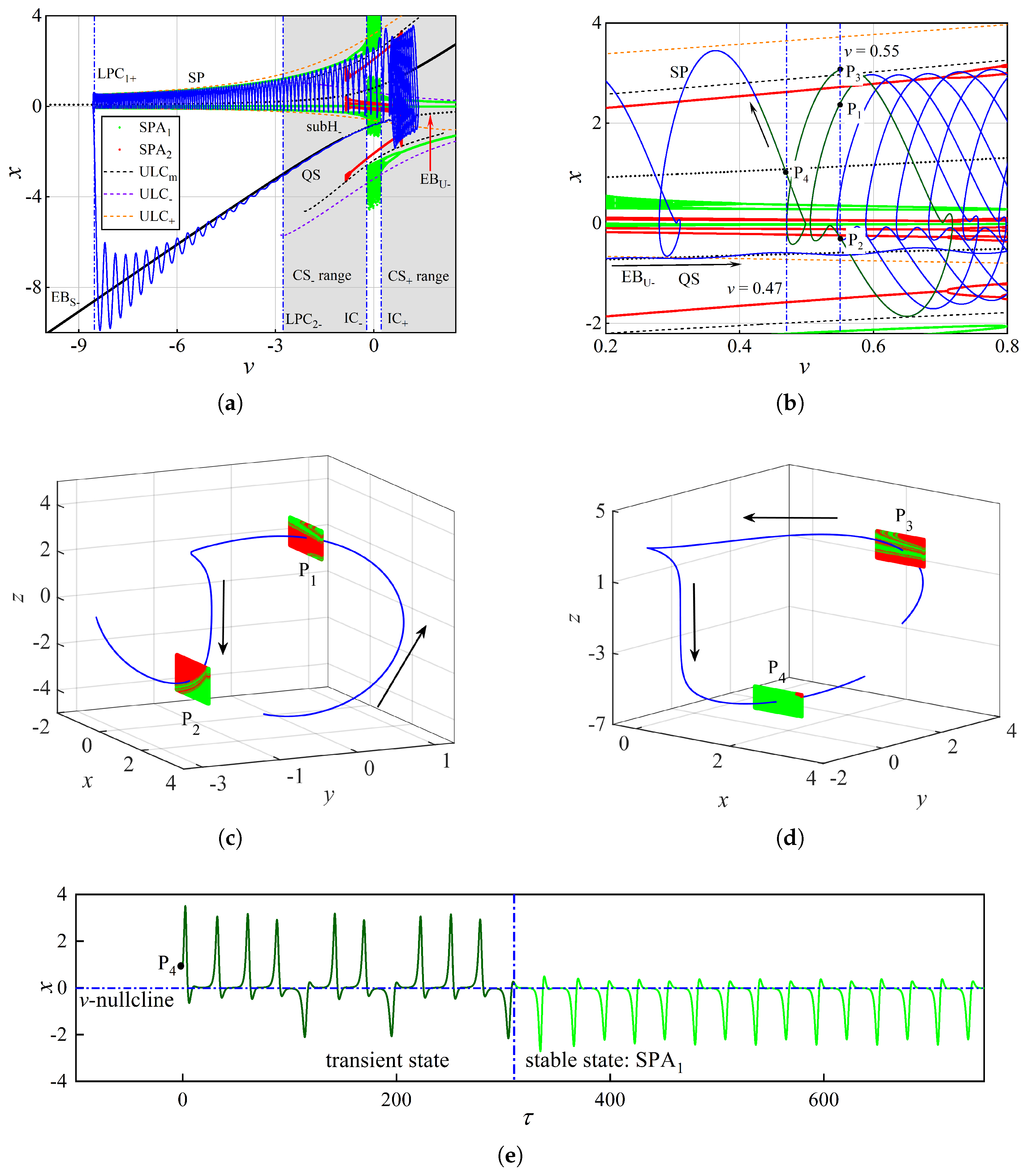
In Figure 9a, we superimpose this bursting behavior on the bifurcation diagram in the $(v,x)$-plane. Here, the trajectory mainly transitions between ${\mathrm{EB}}_{-}$ and the left branch of ${\mathrm{SPA}}_1$, forming a bursting pattern that consists of a single quiescent state $\mathrm{QS}$ and a single spiking state $\mathrm{SP}$. The right branch of ${\mathrm{SPA}}_1$ is not accessed because the slow modulation of v does not drive the trajectory into the corresponding v-range. The two bifurcations ${\mathrm{subH}}_{-}$ and ${\mathrm{LPC}}_{+}$ govern the transition sequences $\mathrm{QS}\to \mathrm{SP}$ and $\mathrm{SP}\to \mathrm{QS}$, respectively. Moreover, the inherent slow passage effect, maintaining the trajectory in the positive-v direction, also allows $\mathrm{QS}$ to extend into the ${\mathrm{CS}}_{+}$ range. Then, similar to the previous case, the trajectory, lifted by ${\mathrm{CS}}_{+}$, exhibits a cluster of large-amplitude oscillations once it transitions to $\mathrm{SP}$. These oscillations are analogous to the transient chaotic trajectories wandering around the saddle-type limit cycle ${\mathrm{ULC}}_{\mathrm{m}}$, thus reversing the bursting evolution path toward the negative-v direction. Subsequently, an abrupt amplitude decrease can also be observed within the bistability regime, consisting of ${\mathrm{SPA}}_1$ and ${\mathrm{SPA}}_2$, ending those large-amplitude oscillations.

However, as shown in Figure 9b, after the abrupt amplitude decrease, the trajectory continues drifting in the negative-v direction, rather than reversing its path, as in the LCDR case. This distinctive evolution process defines the unique bursting structure observed here. The structure also originates from the fractal basin boundaries. To illustrate this via basin analysis, we select four representative points, ${\mathrm{P}}_1$, ${\mathrm{P}}_2$, ${\mathrm{P}}_3$, and ${\mathrm{P}}_4$, along the dark green trajectory, with v-values of $0.55$ and $0.47$, respectively. While traveling from ${\mathrm{P}}_1$ to ${\mathrm{P}}_2$, as shown in Figure 9c, the trajectory within the basin of ${\mathrm{SPA}}_2$ gradually approaches the basin boundaries. After that, the trajectory crosses into the basin of ${\mathrm{SPA}}_1$, represented by ${\mathrm{P}}_3$ and ${\mathrm{P}}_4$ in Figure 9d.

Although the basin result shows that the trajectory should converge to ${\mathrm{SPA}}_1$ upon increasing $\tau$, the chaotic saddle ${\mathrm{CS}}_{+}$ may induce a complex transient state, thus causing the unique structure in this case. To further explain this, we focus on the response of the fast subsystem by setting the initial condition to ${\mathrm{P}}_4$. The time series of x in Figure 9e shows that the fast subsystem maintains a prolonged transient state before completely converging to ${\mathrm{SPA}}_1$. Crucially, in the early stage, this transient state exhibits several oscillations that are predominantly confined to the positive x-half-plane, guaranteeing that the mean $X_{\mathrm{AVER}}$ is positive. Here and throughout this paper, escape refers to the process in which a trajectory leaves the chaotic saddle range in the slow direction before being captured by any coexisting attractor, so that the large-amplitude oscillations are terminated and the trajectory rapidly exits the chaotic saddle range. Supported by this, the full-system trajectory rapidly escapes the ${\mathrm{CS}}_{+}$ range along the negative-v direction before ultimately converging to ${\mathrm{SPA}}_1$.

As a result, the chaotic saddle ${\mathrm{CS}}_{+}$ lifts the trajectory into a cluster of large-amplitude oscillations, reversing the bursting evolution path, while the induced transient state enables the trajectory to then escape the ${\mathrm{CS}}_{+}$ range. We name this bursting behavior the hidden delayed-subH/LPC bursting with lift-escape single-reversal (LESR).

4.3. Hidden Delayed-subH/LPC Bursting with Direct-Captured No-Reversal (DCNR)

To further discuss the regulation of the bursting pattern by the chaotic saddle dynamics, we now consider the response of the full system at $\beta =0.0192$. In this case, the full system exhibits a symmetric bursting behavior consisting of two quiescent states and two spiking states, labeled ${\mathrm{QS}}_i$ and ${\mathrm{SP}}_i$ ($i=1,2$), respectively.

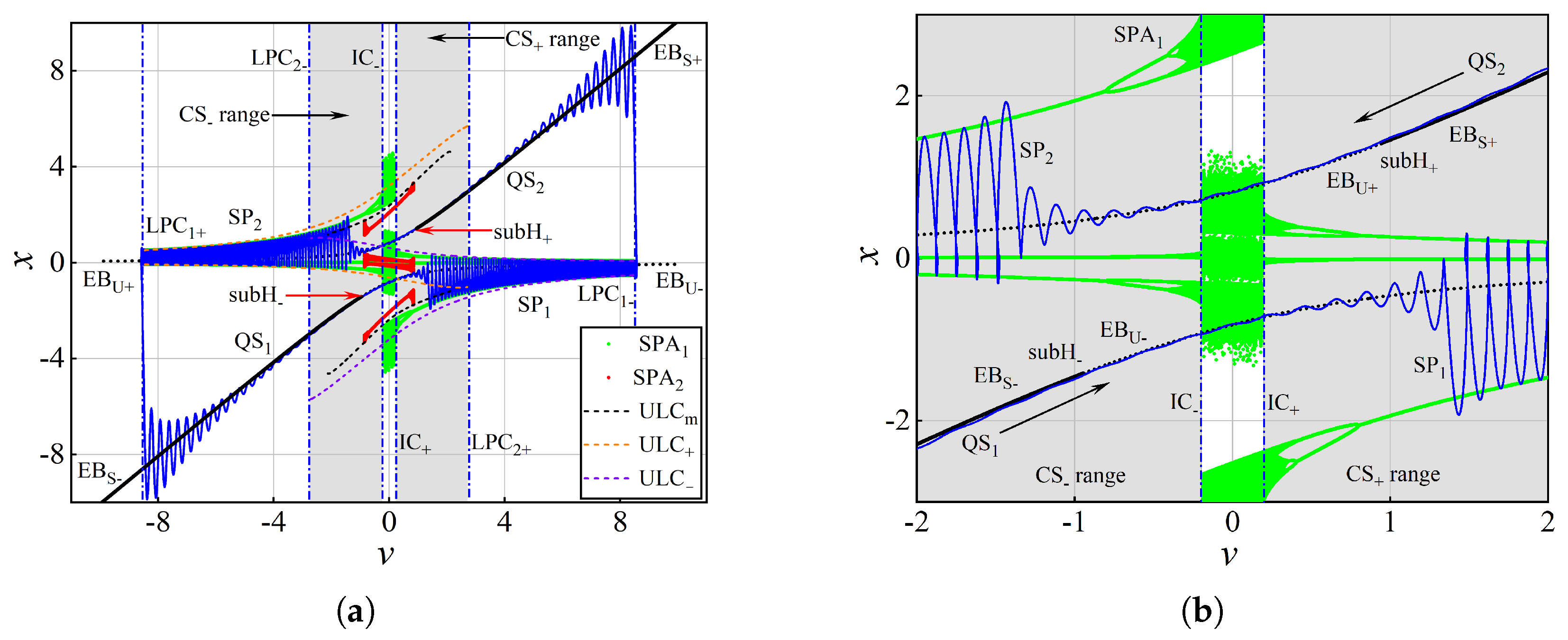
Superimposing this bursting trajectory on the bifurcation diagram, we perform the slow–fast analysis in Figure 10. From Figure 10a, this bursting pattern closely resembles the LCDR case at $\beta =0.02$. The transitions between quiescent and spiking states are governed by the subcritical Hopf bifurcations and the folds of limit cycles. However, in contrast to the previous two cases, there are no large-amplitude oscillations within the chaotic saddle ranges. As shown in Figure 10b, during the two symmetric transitions ${\mathrm{QS}}_1\to {\mathrm{SP}}_1$ and ${\mathrm{QS}}_2\to {\mathrm{SP}}_2$, the trajectories enter ${\mathrm{SP}}_1$ and ${\mathrm{SP}}_2$ by being directly captured by ${\mathrm{SPA}}_1$, rather than being first lifted by ${\mathrm{CS}}_{\pm }$. This can be understood through the basin analysis in Figure 4. Although that analysis was performed at a fixed $v=1.15$, the underlying mechanism applies here. When the trajectory enters the ${\mathrm{CS}}_{+}$ range near ${\mathrm{EP}}_{\mathrm{U}-}$, it can converge directly to ${\mathrm{SPA}}_1$ without undergoing a prolonged transient excursion on the chaotic saddle, as illustrated by trajectory T1 in Figure 4b. After converging to ${\mathrm{SPA}}_1$, the full-system trajectory oscillates along the right and left branches of ${\mathrm{SPA}}_1$, exhibiting ${\mathrm{SP}}_1$ and ${\mathrm{SP}}_2$, respectively.

As mentioned earlier, the right branch of ${\mathrm{SPA}}_1$ yields a positive $X_{\mathrm{AVER}}$, while the left branch yields a negative $X_{\mathrm{AVER}}$. Regulated by the slow-subsystem dynamics under this condition, this bursting pattern maintains its evolution path unchanged after the transitions from quiescent to spiking states. Thus, there is no reversal of the bursting evolution path within the two chaotic saddle ranges. We denote this bursting pattern as the hidden delayed-subH/LPC bursting with direct-captured no-reversal (DCNR).

4.4. Hidden Bursting Patterns with Compound-Path Modes

The three bursting patterns analyzed above correspond to the three distinct transition-path modes within the chaotic saddle ranges: LCDR at $\beta =0.02$, LESR at $\beta =0.01984$, and DCNR at $\beta =0.0192$. Each of these patterns exhibits only a single path mode. However, the dynamical complexity induced by the chaotic saddles suggests that bursting patterns may exist that combine different path modes within a single episode. Two illustrative cases are presented in Figure 11.

At $\beta =0.01972$, we observe an asymmetric periodic bursting pattern that combines two different path modes, as shown in Figure 11a,c. Within a single bursting episode, the trajectory transitions between two quiescent states, ${\mathrm{QS}}_1$ and ${\mathrm{QS}}_2$, and two spiking states, ${\mathrm{SP}}_1$ and ${\mathrm{SP}}_2$. This bursting pattern sequentially exhibits the LCDR path mode within the ${\mathrm{CS}}_{+}$ range and the DCNR path mode within the ${\mathrm{CS}}_{-}$ range.

At $\beta =0.01826$, the full system exhibits an asymmetric periodic bursting pattern that combines three distinct path modes, as shown in Figure 11b,d. This bursting pattern exhibits a combination of the cases at $\beta =0.01984$ (LESR) and $\beta =0.01972$ (LCDR and DCNR). Specifically, while alternating among three quiescent states, ${\mathrm{QS}}_1$, ${\mathrm{QS}}_2$ and ${\mathrm{QS}}_3$, and three spiking states, ${\mathrm{SP}}_1$, ${\mathrm{SP}}_2$, and ${\mathrm{SP}}_3$, it undergoes the path sequence LCDR → DCNR → LESR.

In classical slow–fast systems, a bursting pattern that involves multiple bifurcation mechanisms within a single episode is termed a compound bursting pattern [43,44]. By analogy, the bursting patterns identified here, which combine distinct transition-path modes, are referred to as hidden bursting patterns with compound modes.

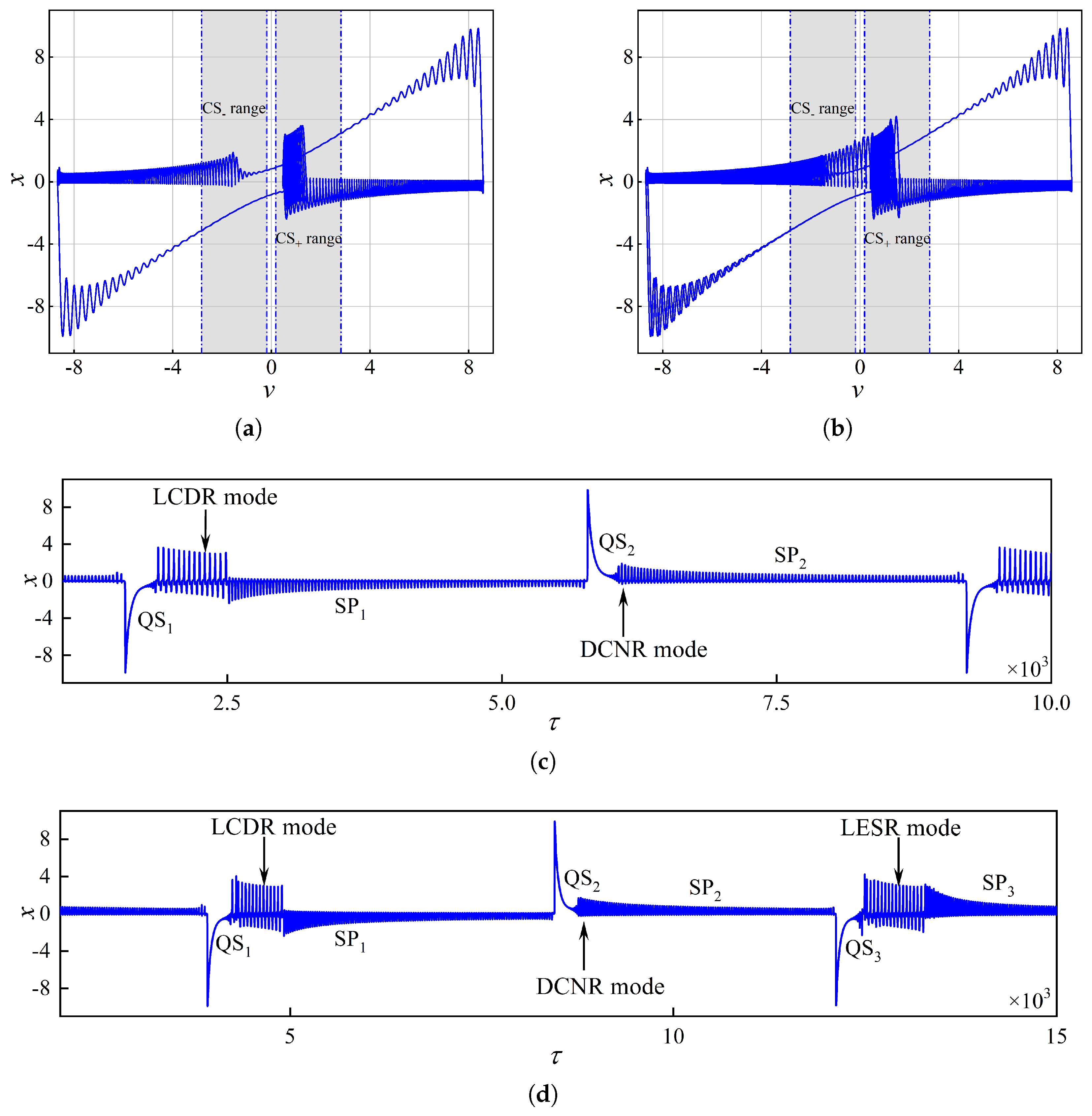
As shown in the full-system Lyapunov exponent spectrum (Figure 7), the full system displays frequent alternations between periodic and chaotic behaviors. Thus, among the compound-path bursting patterns, a particularly significant case is chaotic bursting behavior, which is ergodic among the three transition-path modes investigated above. For instance, as shown in Figure 12, the full system at $\beta =0.01322$ exhibits chaotic bursting, as confirmed by its positive largest Lyapunov exponent in Table A3. Combining the phase portrait in Figure 12a with the time series of x in Figure 12b, we find that this chaotic bursting behavior differs fundamentally from the globally irregular chaos in single-timescale systems. Here, the irregular behavior is mainly confined to the chaotic saddle ranges.

To further illustrate this irregular behavior, we analyze the slow dynamics using the time series of v in Figure 12c. The result shows that the three path modes randomly emerge within the two chaotic saddle ranges. Together with the structural differences induced by sensitivity to initial conditions within the chaotic saddle ranges, this distinct random behavior produces the chaotic compound bursting pattern at $\beta =0.01322$.

In summary, the slow–fast analysis revealed that the hidden bursting oscillations are fundamentally shaped by the dynamical properties of the chaotic saddles ${\mathrm{CS}}_{\pm }$. Within the chaotic saddle ranges, the bursting trajectories can exhibit three distinct transition-path modes, LCDR, LESR, or DCNR, depending on whether the trajectory is lifted, escapes, or is directly captured. Furthermore, these modes can be sequentially combined within a single bursting episode, leading to compound bursting patterns. In the most complex case, the trajectory becomes ergodic among these modes, giving rise to chaotic bursting. These results demonstrate that chaotic saddle dynamics, rather than merely acting as transient noise, serve as an active regulatory mechanism that determines the selection of bursting pathways in the fast subsystem, thereby distinguishing our mechanism from those driven solely by stable invariant sets.

4.5. Mode Identification over a Continuous Parameter Interval

In the preceding subsections, we revealed the hidden bursting patterns of the LCDR, LESR, and DCNR, as well as their compound-path modes for specific values of $\beta$, through slow–fast decomposition, Lyapunov spectrum, and basin analysis. To systematically distinguish these modes over a continuous parameter interval, this subsection proposes an identification method based on the one-dimensional bifurcation diagram of the Poincaré section.

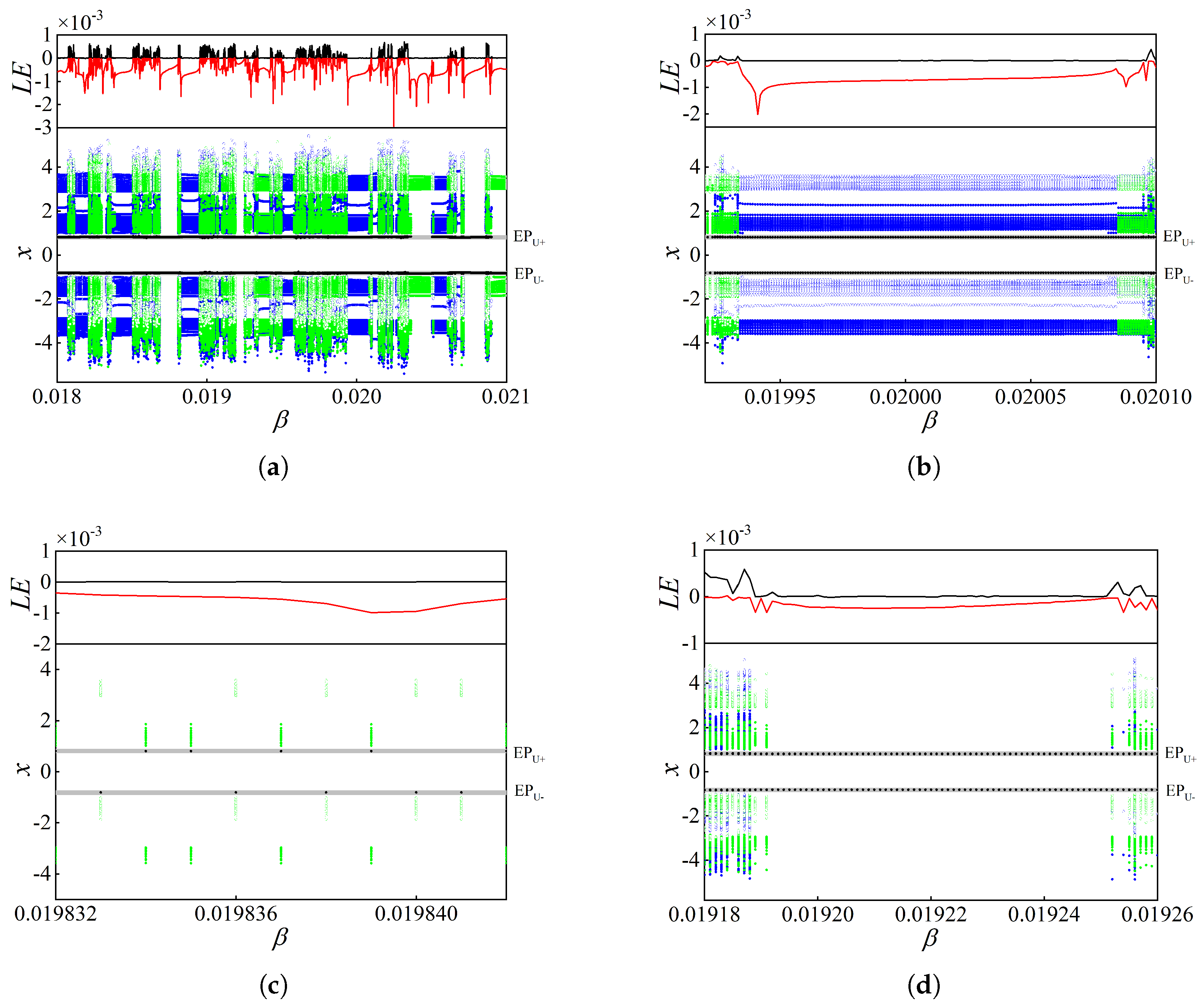
In the hidden bursting behaviors presented in this paper, the slow passage effect drives trajectories across $v=0$ along the unstable equilibrium branches ${\mathrm{EB}}_{U+}$ or ${\mathrm{EB}}_{U-}$. They subsequently enter the corresponding chaotic saddle ranges ${\mathrm{CS}}_{-}$ or ${\mathrm{CS}}_{+}$, within which they complete the quiescent-to-spiking transitions. Once these transitions occur, the trajectories undergo the three distinct transition-path modes presented in Figure 8a (LCDR), Figure 9a (LESR), and Figure 10a (DCNR). Among these modes, chaotic-saddle-induced large-amplitude oscillations are observed in both the LCDR and LESR modes, distinguishing them from the DCNR mode, which exhibits only relatively small-amplitude oscillations. Crucially, trajectories in the LCDR and LESR modes exit the chaotic saddle ranges at $v\approx \pm 2.8282$ and $v\approx \pm 0.1859$, respectively. These two exit thresholds therefore provide a geometric criterion for separating the LCDR mode from the LESR mode.

Based on the above dynamical and geometric features, the transition-path mode for a quiescent-to-spiking transition in system (2) can be identified through the following two-step procedure. First, a Poincaré section is established at $v=0$ to detect the quiescent state, which is identified when the trajectory transversely crosses this section in a small neighborhood of either ${\mathrm{EB}}_{U\pm }$. Second, once a quiescent state is successfully detected, the subsequent spiking state is examined to determine whether chaotic-saddle-induced large-amplitude oscillations are present. If such oscillations are absent, the transition-path mode is identified as DCNR. If they are present, the location at which the trajectory exits the corresponding chaotic saddle region is then extracted: an exit near $v\approx \pm 2.8282$ identifies the LCDR mode, whereas an exit near $v\approx \pm 0.1859$ identifies the LESR mode. This Poincaré bifurcation diagram, complemented by the Lyapunov spectrum, thus provides a systematic framework for identifying bursting modes over a continuous interval of $\beta$.

Figure 13a presents the identification of bursting modes for $\beta \in [0.018,0.021]$. As shown at $\beta =0.02$ in Figure 13b, the single black point near each saddle focus ${\mathrm{EP}}_{U\pm }$ corresponds to the two quiescent states of the periodic bursting behavior presented in Figure 8a, while the filled and open blue dots represent the LCDR mode within the ${\mathrm{CS}}_{-}$ and ${\mathrm{CS}}_{+}$ ranges, respectively. At $\beta =0.01984$ in Figure 13c, only a single black point is detected near ${\mathrm{EP}}_{U-}$ at $v=0$, representing the single quiescent state of the periodic bursting behavior in Figure 9a, while the open green dots represent the LESR mode within the ${\mathrm{CS}}_{+}$ range. As seen at $\beta =0.0192$ in Figure 13d, the two quiescent states in Figure 10a are characterized by the two black points near ${\mathrm{EP}}_{U\pm }$, and the absence of the chaotic-saddle-induced large-amplitude oscillations corresponds to the DCNR mode of this periodic bursting behavior. The above analysis shows that the one-parameter bifurcation diagram (Figure 13a) successfully identifies the periodic bursting behaviors observed in Section 4.1, Section 4.2 and Section 4.3.

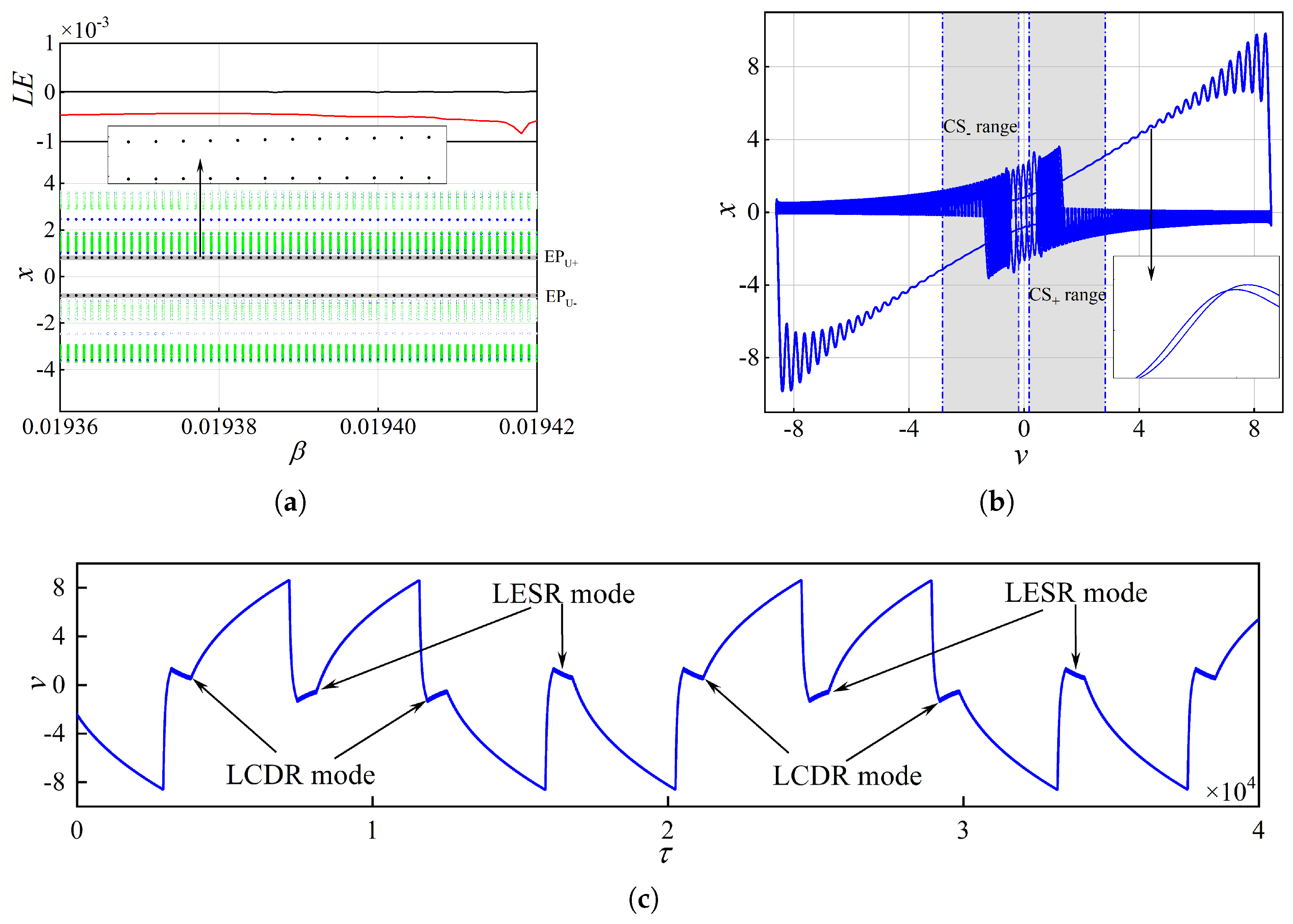
Furthermore, another symmetrical periodic bursting behavior with compound-path mode, distinguished from the two cases presented in Figure 11, can be identified when we apply the proposed method on $\beta \in [0.01936,0.01946]$. As shown in Figure 14a, a pair of black points near each ${\mathrm{EP}}_{U\pm }$ can be observed at a fixed $\beta$, indicating that the quiescent-to-spiking transition occurs twice in each chaotic saddle range. Meanwhile, open and filled dots (both blue and green) appear in the ${\mathrm{CS}}_{+}$ and ${\mathrm{CS}}_{-}$ ranges, respectively, indicating that both the LCDR and LESR modes occur in each chaotic saddle range. Consequently, the newly identified compound bursting behavior exhibits a combination of the LCDR and LESR modes. As confirmed by the phase portrait (Figure 14b) and the time series (Figure 14c) at $\beta =0.0194$, this compound bursting mode follows the following transition sequence in each period: LCDR (${\mathrm{CS}}_{+}$) → LESR (${\mathrm{CS}}_{-}$) → LCDR (${\mathrm{CS}}_{-}$) → LESR (${\mathrm{CS}}_{+}$).

Based on the above results, the chaotic-saddle-organized bursting modes over a continuous interval of $\beta$ can be systematically identified using the proposed method. In particular, this method is highly effective for identifying periodic bursting behaviors in which the quiescent-to-spiking transition occurs no more than twice in each chaotic saddle range. For chaotic bursting behaviors, this method remains applicable since it incorporates the Lyapunov spectrum. However, for more complicated periodic bursting behaviors where the quiescent-to-spiking transition occurs more than twice in each chaotic saddle range, this method requires further improvement by introducing additional information, such as temporal information.

5. Conclusions and Discussions

Through the analysis of a 4D slow–fast system with no equilibria, we have revealed the chaotic-saddle-organized bursting mechanism. Our main findings are as follows. First, two chaotic saddle ranges are identified in the fast subsystem, where intertwined unstable limit cycles and their heteroclinic connections form the skeleton of the chaotic saddles, inducing highly fractal basin boundaries ($D_0=1.85\pm 0.02$). Second, by varying the slow adaptation strength $\beta$, three distinct transition-path modes emerge within the chaotic saddle ranges: lift-captured double-reversal (LCDR), lift-escape single-reversal (LESR), and direct-captured no-reversal (DCNR). The full system can exhibit each mode individually or combine them into compound-path bursting patterns. These modes demonstrate that chaotic saddle dynamics actively select and organize bursting dynamics, while the Lyapunov spectrum confirms the frequent alternations between periodic and chaotic windows underlying this complex behavior.

In most previous studies, bursting dynamics are interpreted within the framework of slow–fast systems, where quiescent and spiking states are attributed to the stable invariant sets of the fast subsystem and their bifurcations. Our work extends this classical paradigm to hidden bursting in slow–fast systems with no equilibria. Specifically, we demonstrate that although the quiescent state remains sustained by the equilibrium branches of the fast subsystem, the subsequent transition from the quiescent to the spiking state is actively organized by the chaotic saddle in a regime where it coexists with a persistent spike attractor. This finding reveals that non-attracting invariant sets can also give rise to rich bursting dynamics. More broadly, it suggests that in the study of bursting dynamics, attention should not be confined solely to stable invariant sets and their bifurcations; the roles of non-attracting invariant sets and their dynamical behaviors deserve equal consideration. The chaotic saddle uncovered here also provides a generic mechanism for complex long transients: trajectories in its vicinity exhibit prolonged irregular oscillations before converging. This suggests that similar hidden bursting may underlie transient phenomena in other multiscale systems. Nevertheless, several questions remain open for further investigation. For instance, the present study is limited to a single-parameter analysis of the fast-subsystem dynamics, particularly the chaotic saddles, as modulated by the slow variable. Moreover, whether systems with no equilibria possess unique hidden bursting mechanisms remains an open question. Furthermore, synchronization control is a fundamental topic in bursting dynamics [45,46]. Thus, investigating how chaotic-saddle-organized bursting dynamics behave in coupled systems and how they influence network-level synchronization would be a valuable direction for future research.

In contrast to the IFOC induction-motor system studied by Kemnang Tsafack et al. [47], where bursting arises from saddle-node and Hopf bifurcations of stable invariant sets in an externally driven model with equilibria, the bursting reported here is organized by a chaotic saddle in an autonomous slow–fast system with no equilibria, so that all bounded oscillations are hidden. Moreover, the transition-path modes identified here (LCDR, LESR, and DCNR) are not present in the motor system, where bursting is classified by conventional bifurcation scenarios. It should be noted that the present study is devoted to the dynamical mechanism of chaotic-saddle-organized hidden bursting, and no circuit implementation is attempted here. A circuit realization of system (2) and a Simulink-based verification, following the approach in Ref. [48], will be an interesting direction for future work.

References

1. Leonov, G.A.; Kuznetsov, N.V. Hidden attractors in dynamical systems. From hidden oscillations in Hilbert-Kolmogorov, Aizerman, and Kalman problems to hidden chaotic attractor in Chua circuits. Int. J. Bifurc. Chaos 2013, 23, 1330002. [Google Scholar] [CrossRef] [Scilit]
2. Hilbert, D. Mathematical problems. Bull. Am. Math. Soc. 1902, 8, 437–479. [Google Scholar] [CrossRef] [Scilit]
3. Bautin, N. The number of limit cycles originating in a case of variable coefficients of an equilibrium state of focus or center type. C. R. Acad. Bulg. Sci. 1939, 24, 669–672. [Google Scholar]
4. Kuznetsov, N.V.; Leonov, G.A.; Vagaitsev, V.I. Analytical-numerical method for attractor localization of generalized Chua’s system. IFAC Proc. Vol. 2010, 43, 29–33. [Google Scholar] [CrossRef] [Scilit]
5. Leonov, G.A.; Kuznetsov, N.V.; Vagaitsev, V.I. Localization of hidden Chua’s attractors. Phys. Lett. A 2011, 375, 2230–2233. [Google Scholar] [CrossRef] [Scilit]
6. Bragin, V.O.; Vagaitsev, V.I.; Kuznetsov, N.V.; Leonov, G.A. Algorithms for finding hidden oscillations in nonlinear systems. The Aizerman and Kalman conjectures and Chua’s circuits. J. Comput. Syst. Sci. Int. 2011, 50, 511–543. [Google Scholar] [CrossRef] [Scilit]
7. Leonov, G.A.; Kuznetsov, N.V.; Vagaitsev, V.I. Hidden attractor in smooth Chua systems. Physica D 2012, 241, 1482–1486. [Google Scholar] [CrossRef] [Scilit]
8. Stankevich, N.V.; Kuznetsov, N.V.; Leonov, G.A.; Chua, L.O. Scenario of the birth of hidden attractors in the Chua circuit. Int. J. Bifurc. Chaos 2017, 27, 1730038. [Google Scholar] [CrossRef] [Scilit]
9. Kuznetsov, N.; Mokaev, T.; Kuznetsova, O.; Kudryashova, E. Hidden attractors in Chua circuit: Mathematical theory meets physical experiments. Nonlinear Dyn. 2023, 111, 5859–5887. [Google Scholar] [CrossRef] [Scilit]
10. Kuznetsov, N.V. Theory of hidden oscillations and stability of control systems. J. Comput. Syst. Sci. Int. 2020, 59, 647–668. [Google Scholar] [CrossRef] [Scilit]
11. Guan, X.; Xie, Y. A review on methods for localization of hidden attractors. Nonlinear Dyn. 2025, 113, 22223–22255. [Google Scholar] [CrossRef] [Scilit]
12. Jafari, S.; Sprott, J.C.; Hashemi Golpayegani, S.M.R. Elementary quadratic chaotic flows with no equilibria. Phys. Lett. A 2013, 377, 699–702. [Google Scholar] [CrossRef] [Scilit]
13. Kuznetsov, N.; Leonov, G. Hidden attractors in dynamical systems: Systems with no equilibria, multistability and coexisting attractors. IFAC Proc. Vol. 2014, 47, 5445–5454. [Google Scholar] [CrossRef] [Scilit]
14. Wei, Z.C.; Wang, R.R.; Liu, A.P. A new finding of the existence of hidden hyperchaotic attractors with no equilibria. Math. Comput. Simul. 2014, 100, 13–23. [Google Scholar] [CrossRef] [Scilit]
15. Ahmad, I.; Srisuchinwong, B.; San-Um, W. On the first hyperchaotic hyperjerk system with no equilibria: A simple circuit for hidden attractors. IEEE Access 2018, 6, 35449–35456. [Google Scholar] [CrossRef] [Scilit]
16. Zhang, L.P.; Liu, Y.; Wei, Z.C.; Jiang, H.B.; Bi, Q.S. Hidden attractors in a class of two-dimensional rational memristive maps with no fixed points. Eur. Phys. J. Spec. Top. 2022, 231, 2173–2182. [Google Scholar] [CrossRef] [Scilit]
17. Zhang, S.; Zeng, Y.C. A simple Jerk-like system without equilibrium: Asymmetric coexisting hidden attractors, bursting oscillation and double full Feigenbaum remerging trees. Chaos Solitons Fract. 2019, 120, 25–40. [Google Scholar] [CrossRef] [Scilit]
18. Yan, S.H.; Zhang, Y.Y.; Ren, Y.; Sun, X.; Wang, E.T.; Song, Z.L. Four-dimensional Hindmarsh-Rose neuron model with hidden firing multistability based on two memristors. Phys. Scr. 2022, 97, 125203. [Google Scholar] [CrossRef] [Scilit]
19. Zhang, J.; Hou, J.Y.; Xie, Q.G.; Guo, Y. Circuit realization and application of a chaotic system with hidden attractor, controlled spike discharge and offset boosting. Nonlinear Dyn. 2024, 112, 18551–18579. [Google Scholar] [CrossRef] [Scilit]
20. Rinzel, J. A formal classification of bursting mechanisms in excitable systems. In Mathematical Topics in Population Biology, Morphogenesis and Neurosciences; Teramoto, E., Yamaguti, M., Eds.; Lecture Notes in Biomathematics; Springer: Berlin, Germany, 1987; Volume 71, pp. 267–281. [Google Scholar] [CrossRef] [Scilit]
21. Izhikevich, E.M. Neural excitability, spiking and bursting. Int. J. Bifurc. Chaos 2000, 10, 1171–1266. [Google Scholar] [CrossRef] [Scilit]
22. Izhikevich, E.M.; Desai, N.S.; Walcott, E.C.; Hoppensteadt, F.C. Bursts as a unit of neural information: Selective communication via resonance. Trends Neurosci. 2003, 26, 161–167. [Google Scholar] [CrossRef] [Scilit] [PubMed]
23. Richard, B.; Jonathan, E.R. Multi-timescale systems and fast-slow analysis. Math. Biosci. 2017, 287, 105–121. [Google Scholar] [CrossRef] [Scilit] [PubMed]
24. Ciszak, M.; Marino, F. Type-III intermittency in emergent bursting dynamics of globally coupled rotators. Chaos Solitons Fract. 2025, 194, 116150. [Google Scholar] [CrossRef] [Scilit]
25. Yang, Y.; Jiang, J.J.; Shi, X.H.; Qin, W.J. Bifurcations and the switching of spiking and bursting in the extended Hindmarsh–Rose neuronal system. Adv. Cont. Discr. Mod. 2026, 2026, 63. [Google Scholar] [CrossRef] [Scilit]
26. Duan, L.X.; Chen, X.L.; Xia, L.Y.; Wang, Z.H. Dynamics and control of mixed bursting in nonlinear pre-Bötzinger complex systems. Nonlinear Dyn. 2024, 112, 8539–8556. [Google Scholar] [CrossRef] [Scilit]
27. Ma, F.; Duan, L.X.; Wang, Z.H.; Zhao, Y. Bifurcation and multiple timescale dynamics of mixed bursting in the neuronal model. Eur. Phys. J. B 2024, 97, 95. [Google Scholar] [CrossRef] [Scilit]
28. Zhao, Y.Q.; Liu, M.T.; Shi, X.; Yang, Y.Y. Bifurcation analysis with two slow variables of firing patterns and mixed bursting in respiratory neurons. Nonlinear Dyn. 2026, 114, 599. [Google Scholar] [CrossRef] [Scilit]
29. Zhang, Z.D.; Chen, Z.Y.; Bi, Q.S. Modified slow-fast analysis method for slow-fast dynamical systems with two scales in frequency domain. Theor. Appl. Mech. Lett. 2019, 9, 358–362. [Google Scholar] [CrossRef]
30. Bao, B.C.; Chen, L.H.; Bao, H.; Chen, M.; Xu, Q. Bursting dynamics in a memristive system with slow-fast timescales. Chaos Solitons Fract. 2024, 181, 114608. [Google Scholar] [CrossRef] [Scilit]
31. Lyu, W.P.; Li, S.L.; Chen, Z.Y.; Bi, Q.S. Bursting dynamics in a singular vector field with codimension three triple zero bifurcation. Mathematics 2023, 11, 2486. [Google Scholar] [CrossRef] [Scilit]
32. Jiang, S.P.; Han, X.J.; Yu, H.L. A novel route to bursting by frequency switching in the slowly forced Duffing system. Nonlinear Dyn. 2024, 112, 19013–19022. [Google Scholar] [CrossRef] [Scilit]
33. Wang, K.; Han, N. Bursting oscillations analysis of the irrational pendulum system. Eur. Phys. J. Plus 2025, 140, 648. [Google Scholar] [CrossRef] [Scilit]
34. Zhang, D.J.; Qian, Y.H. Quasi-periodic bursting in a kind of Duffing–Van der Pol system with two excitation terms. J. Vib. Eng. Technol. 2025, 13, 1. [Google Scholar] [CrossRef] [Scilit]
35. Zhang, C.; Wang, Z.X.; Bi, Q.S. Bursting oscillations in a modified Chua’s circuit of Filippov type with double-frequency excitation. Nonlinear Dyn. 2026, 114, 272. [Google Scholar] [CrossRef] [Scilit]
36. Grebogi, C.; Ott, E.; Yorke, J.A. Crises, sudden changes in chaotic attractors, and transient chaos. Physica D 1983, 7, 181–200. [Google Scholar] [CrossRef] [Scilit]
37. Zhao, H.Q.; Ma, X.D.; Bi, Q.S. Chaotic bursting patterns induced by transient chaos in a smooth three-dimensional dynamic model. Int. J. Non-Linear Mech. 2024, 159, 104592. [Google Scholar] [CrossRef] [Scilit]
38. Dhooge, A.; Govaerts, W.; Kuznetsov, Y.A. MATCONT: A MATLAB package for numerical bifurcation analysis of ODEs. ACM Trans. Math. Softw. 2003, 29, 141–164. [Google Scholar] [CrossRef] [Scilit]
39. Grebogi, C.; Ott, E.; Yorke, J.A. Critical exponent of chaotic transients in nonlinear dynamical systems. Phys. Rev. Lett. 1986, 57, 1284–1287. [Google Scholar] [CrossRef] [Scilit] [PubMed]
40. Lai, Y.C.; Winslow, R.L. Geometric properties of the chaotic saddle responsible for supertransients in spatiotemporal chaotic systems. Phys. Rev. Lett. 1995, 74, 5208–5211. [Google Scholar] [CrossRef] [Scilit] [PubMed]
41. Tél, T.; Lai, Y.C. Chaotic saddles and their role in transient chaos. Phys. Rep. 2008, 460, 245–298. [Google Scholar] [CrossRef] [Scilit]
42. Han, X.J.; Bi, Q.S.; Zhang, C.; Yu, Y. Delayed bifurcations to repetitive spiking and classification of delay-induced bursting. Int. J. Bifurc. Chaos 2014, 24, 1450098. [Google Scholar] [CrossRef] [Scilit]
43. Ma, X.D.; Xia, D.X.; Jiang, W.A.; Liu, M.; Bi, Q.S. Compound bursting behaviors in a forced Mathieu-van der Pol-Duffing system. Chaos Solitons Fract. 2021, 147, 110967. [Google Scholar] [CrossRef] [Scilit]
44. Wei, M.K.; Jiang, W.A.; Ma, X.D.; Zhang, X.F.; Han, X.J.; Bi, Q.S. Compound bursting dynamics in a parametrically and externally excited mechanical system. Chaos Solitons Fract. 2021, 143, 110605. [Google Scholar] [CrossRef] [Scilit]
45. Wu, F.Q.; Guo, Y.T.; Ma, J.; Jin, W.Y. Synchronization of bursting memristive Josephson junctions via resistive and magnetic coupling. Appl. Math. Comput. 2023, 456, 128131. [Google Scholar] [CrossRef] [Scilit]
46. Wu, F.Q.; Meng, H.; Ma, J. Reproduced neuron-like excitability and bursting synchronization of memristive Josephson junctions loaded inductor. Neural Netw. 2024, 169, 607–621. [Google Scholar] [CrossRef] [Scilit] [PubMed]
47. Kemnang Tsafack, A.S.; Mboupda Pone, J.R.; Cheukem, A.; Kengne, R.; Kenne, G. Coexisting attractors and bursting oscillations in IFOC of 3-phase induction motor. Eur. Phys. J. Spec. Top. 2020, 229, 989–1006. [Google Scholar] [CrossRef] [Scilit]
48. Liu, X.; Zhao, L.; Jin, J. A noise-tolerant fuzzy-type zeroing neural network for robust synchronization of chaotic systems. Concurr. Comput. Pract. Exper. 2024, 36, e8218. [Google Scholar] [CrossRef] [Scilit]
Figure 1. Self-sustained oscillations with α = 0.02 , β = 0.02 , and δ = 0.4 . (a) Three coexisting limit cycles in the ( v , x ) plane for μ = 0.25 . The initial condition X IN and period T are annotated. (b) Periodic point-cycle bursting in the ( v , x ) plane for μ = 0.6 . (c) Time series of the bursting oscillation in (b). The four traces from top to bottom correspond to x, y, z, and v.
Mathematics 14 03396 g001
Figure 2. Dynamical analysis of the fast subsystem at v = 0 . (a) Invariant sets in the ( x , z ) -plane (left) and spherical basin portrait for SPA 1 and SPA 2 (right). (b) Basins (left) and four representative trajectories (right) near the unstable manifold of EP U .
Mathematics 14 03396 g002
Figure 3. Bifurcation analysis of the invariant sets from Figure 2a, where the unstable limit cycles are represented by maxima of x, and the attractors are represented by extreme values of x. (a) One-parameter bifurcation analysis for saddle-type invariant sets: ULC m and ULC ± (top); EP U ± (bottom). (b) Two-parameter analysis for the bifurcations obtained in (a), plotted in the ( v , μ ) -plane. (c,e) display the analysis for attractors SPA 1 (green dots) and SPA 2 (red dots): largest and second-largest Lyapunov exponents (top), and one-parameter bifurcation diagram (bottom). (d,f) display the local enlargements of (c,e), respectively.
Mathematics 14 03396 g003
Figure 4. Dynamical analysis of the fast subsystem at v = 1.15 . (a) Invariant sets in the ( x , z ) -plane (left) and spherical basin portrait for SPA 1 and SPA CS (right). The transient chaotic trajectory TC (dark green), extracted from T 4 in (b), approximates the structure of CS + . (b) Basins (left) and four representative trajectories (right) near the unstable manifold of EP U .
Mathematics 14 03396 g004
Figure 5. Transient lifetime statistics from spherical sprinkling at ULC m . (a) Escape-time distribution P ( τ ) for N = 100,000 (blue squares) and N = 500,000 (red triangles) initial conditions. (b) Exponential fits of log P ( τ ) versus τ over the regime τ [ 500 , 2500 ] . Least-squares fits give escape rates κ = 0.00454 ± 0.00013 ( N = 100,000 , R 2 = 0.9932 ) and κ = 0.00457 ± 0.00007 ( N = 500,000 , R 2 = 0.9993 ), agreeing within 0.63 % .
Mathematics 14 03396 g005
Figure 6. Basins (left) and two representative trajectories (right) near the unstable manifold of EP U at v = 3.2 , where the basin of EP S + and the related transient trajectory are colored in light gray.
Mathematics 14 03396 g006
Figure 7. Lyapunov exponents of the full system with respect to β . (a) β [ 0.01 , 0.023 ] ; (b) local magnification of (a) within β [ 0.018 , 0.02 ] ; (c) convergence of the largest Lyapunov exponent LE 1 at β = 0.01322 as a function of the integration time τ ; (d) local magnification of (c) for τ 2 × 10 5 . In (c), the first 5 × 10 4 time units are discarded as transient, and the exponent is computed over a total of 4 × 10 5 time units. In (d), LE 1 converges to a constant positive value of approximately 0.0008.
Mathematics 14 03396 g007aMathematics 14 03396 g007b
Figure 8. Slow–fast analysis of the periodic bursting pattern at β = 0.02 . (a) Phase portrait superimposed on the bifurcation diagram. (bd) Trajectory segments of Stage I, II, and III within the CS + range, respectively. (e) Basin analysis for point P 1 to P 2 , marked in (c). (f) Basin analysis for point P 3 marked in (c) and P 4 marked in (d).
Mathematics 14 03396 g008
Figure 9. Slow–fast analysis of the periodic bursting pattern at β = 0.01984 . (a) Phase portrait superimposed on bifurcation diagram; (b) local enlargement showing abrupt amplitude decrease; (c,d) basin analyses using the four points marked in (b) as initial conditions; (e) time series of x for the fast subsystem trajectory starting from P 4 .
Mathematics 14 03396 g009
Figure 10. Slow–fast analysis of the periodic bursting pattern at β = 0.0192 . (a) Phase portrait superimposed on bifurcation diagram; (b) Local enlargement near transitions from quiescent states to spiking states.
Mathematics 14 03396 g010
Figure 11. Two distinct periodic compound bursting patterns, where (a,b) respectively display the phase portraits at β = 0.01972 and β = 0.01826 , with corresponding time series of x presented in (c,d).
Mathematics 14 03396 g011
Figure 12. Chaotic compound bursting pattern at β = 0.01322 . (a) Phase portrait in ( v , x ) -plane; (b) Time series of x; (c) Time series of v.
Mathematics 14 03396 g012
Figure 13. Identification of bursting modes via one-parameter bifurcation analysis in β (step size 10 6 ). (Upper panels) Largest and second-largest Lyapunov exponents (from Figure 7). (Lower panels) Poincaré bifurcation diagram in the ( β , x ) -plane. Black dots near the saddle foci EP U ± (thick gray lines, obtained by substituting v = 0 into Equation (9)) indicate quiescent states. Blue and green dots ( | x | > 1 ) denote the extrema of chaotic-saddle-induced large-amplitude oscillations; filled/open blue (green) dots show the LCDR (LESR) mode within CS ( CS + ). (a) β [ 0.018 , 0.021 ] ; (bd) local enlargements for LCDR, LESR, and DCNR modes, respectively.
Mathematics 14 03396 g013
Figure 14. Periodic bursting behavior with the following compound mode sequence: LCDR ( CS + ) → LESR ( CS ) → LCDR ( CS ) → LESR ( CS + ). (a) The identification method applied on β [ 0.01936 , 0.01946 ] ; (b,c) display the phase portrait in the ( v , x ) -plane and the time series of v at β = 0.0194 , respectively.
Mathematics 14 03396 g014
Disclaimer/Publisher’s Note: The statements, opinions and data contained in all publications are solely those of the individual author(s) and contributor(s) and not of MDPI and/or the editor(s). MDPI and/or the editor(s) disclaim responsibility for any injury to people or property resulting from any ideas, methods, instructions or products referred to in the content.