A Composite Evaluation Framework for Dimensionality Reduction Methods in Industry 4.0 Data

Abstract

Dimensionality reduction is essential in industrial analytics, as high-dimensional process data often contain redundant and correlated variables that increase computational burden and model complexity. This study proposes a weighted composite evaluation framework (S_wc) that jointly considers predictive performance, computational execution time, and representation dimensionality when comparing feature selection (FS) and feature extraction (FE) methods. The framework was evaluated on the Tennessee Eastman Process benchmark using seven fault classes, 52 process variables, a common XGBoost classifier, and 10 independently seeded stratified repetitions. Nine FS methods and four FE methods were benchmarked across four operational weighting scenarios: Balanced, Predictive Focus, Efficiency Focus, and Compactness Focus. Among the FE techniques, linear discriminant analysis (LDA) consistently achieved the highest composite score across all scenarios (mean rank = 1.00) due to its high-class separability and minimal computational overhead. For FS methods, forward selection and XGBoost-based selection jointly achieved the leading overall average rank (mean rank = 1.50), with XGBoost leading under predictive- and compactness-focused scenarios, while forward selection led under Balanced and Efficiency Focus constraints. Nonparametric statistical analysis indicated significant overall differences among methods based on the Friedman test (p < 0.05), while no individual pairwise comparison remained significant after Holm correction. The results demonstrate that evaluating methods solely by predictive performance provides an incomplete assessment. The proposed framework serves as a transparent multicriteria decision support mechanism for selecting dimensionality reduction strategies aligned with specific Industry 4.0 operational priorities.

1. Introduction

The continuous development of digital technologies has fundamentally transformed modern manufacturing systems. Within this transformation, Industry 4.0 has introduced highly interconnected and data-driven production environments through the integration of advanced sensing technologies, industrial Internet of Things (IIoT), automation systems, and intelligent data analytics [1,2]. Consequently, modern industrial facilities continuously generate large volumes of heterogeneous data from sensors, machines, controllers, and communication networks. These data provide valuable information about process conditions, equipment behavior, product quality, and operational performance, supporting advanced applications such as fault diagnosis, predictive maintenance, process optimization, and intelligent decision support [3].

However, the increasing dimensionality and complexity of industrial datasets introduce important challenges for machine learning-based analysis. Industrial process data may contain redundant variables, multicollinearity, measurement noise, nonlinear relationships, and complex interactions among process parameters. Such characteristics can increase computational requirements, reduce model interpretability, and introduce unnecessary complexity into predictive models [4]. Consequently, dimensionality reduction is a crucial preprocessing strategy for obtaining more compact representations while retaining information relevant to the prediction task.

Dimensionality reduction methods are generally categorized into feature selection (FS) and feature extraction (FE) approaches [5]. Feature selection identifies a subset of the original variables, thereby preserving their physical meaning and domain interpretability. This property is particularly relevant in industrial applications, where the relationship between process variables and system behavior provides vital information for fault root cause analysis and operational decision-making [4]. Feature extraction, in contrast, transforms original variables into a lower-dimensional latent space. Such transformations provide compact representations of complex datasets, although the resulting features may be less directly interpretable in terms of physical process parameters [6,7].

A wide range of feature selection methods has been developed, broadly categorized into filter, wrapper, and embedded approaches. Filter methods such as Pearson correlation and mutual information evaluate feature relevance using statistical or information theoretic criteria, providing computationally efficient dimensionality reduction [4,5,8]. Wrapper methods evaluate candidate feature subsets according to the performance of a predictive model and can account for complex variable interactions, although their computational requirements are typically higher [9,10]. Embedded approaches perform feature selection inherently during the model training process. Representative examples include LASSO, elastic net, random forest, and XGBoost, which incorporate variable selection or importance scoring directly into the learning procedure [11,12,13,14].

Feature extraction methods provide an alternative strategy by constructing a new representation from original variables. Principal component analysis (PCA) is one of the most widely used linear dimensionality reduction techniques, providing a representation based on directions of maximum variance [15]. Linear discriminant analysis (LDA) performs supervised dimensionality reduction by seeking directions that enhance class separability and has been extensively applied in classification tasks [16,17]. In multivariate statistical modeling, methods such as partial least squares regression (PLSR) have also addressed relationships between predictor and response variables [18,19]. Furthermore, nonlinear and deep learning approaches, including Kernel PCA, t-SNE, UMAP, and autoencoders, provide powerful alternative representations for datasets containing nonlinear structures [6,20,21,22].

Although these methods have been extensively investigated, their effectiveness is commonly assessed using a limited number of performance indicators. Predictive performance is frequently emphasized, whereas computational cost and representation compactness receive less systematic attention. In practical industrial applications, however, these criteria can directly conflict. A method providing high predictive performance may retain a relatively large number of variables or require substantial computational time, whereas a highly compact method may reduce processing requirements at the expense of classification accuracy. Therefore, comparing dimensionality reduction strategies requires evaluating multiple criteria simultaneously rather than relying on predictive performance alone.

Multicriteria evaluation provides a systematic framework for comparing alternatives when several potentially conflicting objectives must be balanced [23]. For dimensionality reduction, predictive performance acts as a benefit criterion, whereas computational time and representation dimensionality serve as cost criteria. Integrating these criteria into a unified composite evaluation score provides a more informative basis for comparing alternative dimensionality reduction strategies than single metric evaluations [24,25].

Motivated by this requirement, this study proposes a weighted composite evaluation framework for the comparative assessment of dimensionality reduction methods in industrial fault diagnosis. Rather than introducing a new feature selection or extraction algorithm, this study focuses on establishing a unified decision support framework to evaluate representations according to three complementary aspects: predictive performance, computational efficiency, and representation compactness. The framework combines these criteria into a single composite score (S_wc), allowing the explicit control of relative priorities across operational weighting scenarios.

The proposed framework is evaluated on the Tennessee Eastman Process (TEP) benchmark dataset, a standard baseline for industrial process monitoring and fault diagnosis research. The dataset provides a challenging multiclass classification environment characterized by 52 continuous process variables across multiple operational fault categories. Representative feature selection methods (covering filter, wrapper, and embedded strategies) and feature extraction methods (linear, nonlinear, and deep learning techniques) are evaluated under a common experimental protocol using a fixed XGBoost classifier and 10 independently seeded stratified train–test repetitions.

The main contributions of this study are threefold:

• A unified composite evaluation framework (S_wc) is developed to evaluate dimensionality reduction methods by simultaneously integrating predictive capability, computational time, and feature space dimensionality.
• Comprehensive FS and FE strategies are benchmarked under a strictly controlled experimental protocol using the same industrial benchmark dataset, classification model, and repeated stratified evaluation procedure, enabling rigorous cross-method comparisons.
• Sensitivity analysis across four operational weighting scenarios (Balanced, Predictive Focus, Efficiency Focus, and Compactness Focus), along with nonparametric statistical testing, is conducted to evaluate rank stability and practical trade-offs under shifting operational priorities.

The remainder of this paper is organized as follows. Section 2 presents the theoretical background of the evaluated dimensionality reduction methods. Section 3 describes the proposed composite evaluation framework and experimental methodology. Section 4 presents the experimental results, sensitivity analyses, and statistical evaluations. Section 5 discusses the findings and their practical implications. Finally, Section 6 concludes the study and outlines future research directions.

2. Dimensionality Reduction Methods for Industry 4.0 Applications

Industry 4.0 has introduced highly interconnected manufacturing environments in which large-scale data are continuously generated from sensors, machines, controllers, and industrial communication systems [1,2,3]. The increasing dimensionality of industrial datasets creates challenges related to computational efficiency, redundant information, noise accumulation, and model interpretability. Therefore, dimensionality reduction has become an essential approach for improving the efficiency and reliability of industrial data analytics systems [3,26].

Dimensionality reduction techniques are generally classified into two main categories: feature selection and feature extraction [5]. Feature selection identifies informative variables from the original feature space while preserving their physical meaning, making it particularly suitable for interpretable industrial applications. Feature extraction, in contrast, transforms original variables into lower-dimensional latent representations through linear or nonlinear mappings, which can provide improved representation capability but may reduce direct interpretability [6].

Feature selection approaches are commonly divided into filter-based, wrapper-based, and embedded methods according to their relationship with the predictive model [4,27]. Filter methods evaluate feature relevance using statistical criteria, wrapper methods search for optimal feature subsets based on model performance, and embedded methods perform feature selection during model training. Representative approaches used in industrial analytics are summarized in

Table 1. Representative feature selection strategies considered in industrial analytics.

Category	Representative Methods	Main Advantage	Main Limitation
Filter-Based	Pearson Correlation, Mutual Information	Computationally efficient and scalable; independent of the predictive model	Feature interactions and model-specific relationships are not considered
Wrapper-Based	Forward Selection, Backward Selection, Recursive Feature Elimination (RFE)	Considers feature interactions and directly optimizes predictive performance	Computationally demanding due to repeated model evaluation
Embedded	LASSO, Elastic Net, Random Forest, XGBoost	Integrates feature selection with model training and provides a balance between accuracy and efficiency	Performance depends on the underlying learning algorithm

.

Feature extraction methods include linear transformation techniques, nonlinear manifold learning approaches, and deep learning-based representations. Linear methods such as principal component analysis (PCA) and linear discriminant analysis (LDA) provide computational efficiency and interpretability, whereas nonlinear approaches such as UMAP and autoencoders are capable of capturing complex relationships in high-dimensional industrial data [20,21,28]. Representative feature extraction methods are presented in

Table 2. Representative feature extraction strategies considered in industrial analytics.

Category	Representative Methods	Representation Type	Main Characteristics
Linear Methods	PCA, LDA	Linear latent transformation	Computationally efficient and interpretable; may be limited in capturing nonlinear relationships
Nonlinear Manifold Methods	Uniform Manifold Approximation and Projection (UMAP)	Nonlinear latent representation	Captures complex data structures while preserving local and global relationships
Deep Learning-Based Methods	Autoencoder	Deep nonlinear latent representation	Learns hierarchical features but requires higher computational resources and reduces interpretability

.

2.1. Feature Selection Methods

Feature selection aims to identify a compact subset of informative variables while eliminating irrelevant, redundant, and noisy features from high-dimensional datasets. In industrial analytics, feature selection contributes to improved computational efficiency, enhanced model interpretability, and reduced overfitting risk. Existing feature selection approaches are generally categorized into filter-based, wrapper-based, optimization-assisted, and embedded methodologies according to their interaction with predictive learning algorithms [4,27,29].

2.1.1. Filter-Based Methods

Filter-based methods evaluate feature relevance independently of the predictive learning algorithm by relying on statistical or information theoretic criteria. Due to their computational efficiency and scalability, these methods are frequently utilized as preprocessing tools in high-dimensional industrial datasets. Common filter approaches include Pearson correlation analysis and mutual information (MI) [4,5,8].

Pearson correlation analysis measures linear dependency between variables and is widely utilized for redundancy elimination and multicollinearity reduction in industrial datasets. The Pearson correlation coefficient is defined as [30]:

$${\mathrm{r}}_{\mathrm{x}\mathrm{y}}={\displaystyle \frac{{\displaystyle \sum _{\mathrm{i}=1}^{\mathrm{n}}\left({\mathrm{x}}_{\mathrm{i}}-\overline{\mathrm{x}}\right)\left({\mathrm{y}}_{\mathrm{i}}-\overline{\mathrm{y}}\right)}}{\sqrt{{\displaystyle \sum _{\mathrm{i}=1}^{\mathrm{n}}{\left({\mathrm{x}}_{\mathrm{i}}-\overline{\mathrm{x}}\right)}^2{\displaystyle \sum _{\mathrm{i}=1}^{\mathrm{n}}{\left({\mathrm{y}}_{\mathrm{i}}-\overline{\mathrm{y}}\right)}^2}}}}}$$

(1)

Here, x_i and y_i represent the observed values of variables X and Y, respectively, whereas $\overline{\mathrm{x}}$ and $\overline{\mathrm{y}}$ denote their corresponding sample means. Features exhibiting excessively high correlation structures may introduce redundant information and negatively affect model stability.

Unlike correlation-based approaches, mutual information captures both linear and nonlinear dependency structures by quantifying the amount of shared information between variables [31,32,33].

If X and Y are continuous random variables, the joint density function is p(x, y), and the marginal densities are p_X(x) and p_Y(y), then MI is written as:

$$\mathrm{M}\mathrm{I}(\mathrm{X};\mathrm{Y})={\displaystyle \underset{\mathrm{x}}{\int }{\displaystyle \underset{\mathrm{y}}{\int }\mathrm{p}(\mathrm{x},\mathrm{y})\log \frac{\mathrm{p}(\mathrm{x},\mathrm{y})}{{\mathrm{p}}_{\mathrm{X}}(\mathrm{x}){\mathrm{p}}_{\mathrm{Y}}(\mathrm{y})}}}\mathrm{d}\mathrm{y}\mathrm{d}\mathrm{x}.$$

(2)

Because MI does not assume linear relationships, it is particularly advantageous for industrial sensor datasets characterized by nonlinear operational dependencies [5]. However, filter-based approaches generally ignore feature interactions and classifier-specific relationships, potentially excluding feature combinations that may collectively contain important predictive information.

2.1.2. Wrapper-Based Methods

Wrapper-based feature selection approaches evaluate candidate feature subsets directly according to predictive model performance. Unlike filter-based approaches, wrapper methods explicitly account for feature interactions and classifier-specific relationships, thereby often achieving superior predictive capability [10]. However, repeated model training substantially increases computational complexity, particularly in high-dimensional industrial datasets.

Among wrapper methods, forward selection (FS) and backward selection (BS) are the most widely used search strategies. FS begins with an empty feature subset and sequentially adds the variable that provides the greatest improvement in model performance, whereas BS starts with the complete feature set and iteratively removes the least informative variables according to criteria such as accuracy, R², AIC, or BIC [9,34]. These approaches are frequently applied in Industry 4.0 environments because they preserve interpretability while improving predictive performance in applications such as fault diagnosis, quality monitoring, and process optimization [1,35].

Recursive feature elimination (RFE) is another wrapper-based technique that iteratively removes the least informative variables according to model-specific importance scores until an optimal feature subset is obtained. Although RFE frequently improves classification and prediction performance, its computational cost may become substantial for large-scale industrial applications involving thousands of variables [36].

2.1.3. Embedded-Based Methods

Embedded methods integrate feature selection directly into the model optimization process, thereby balancing predictive performance and computational efficiency. These methods are particularly suitable for industrial datasets characterized by high dimensionality, multicollinearity, and sparse variable structures.

Random forest (RF) estimates feature importance according to impurity reduction obtained during tree construction, whereas Extreme Gradient Boosting (XGBoost) evaluates feature contribution through gradient-boosted optimization mechanisms [11,12,26,37]. Because these approaches perform feature evaluation during model construction, they provide computational advantages compared with iterative wrapper-based strategies.

Regularization-based approaches such as LASSO and elastic net simultaneously perform coefficient estimation and feature selection by penalizing model complexity [13,14,38]. LASSO introduces an L1 regularization penalty that forces some regression coefficients toward zero, thereby eliminating noninformative variables. Mathematically, the LASSO, ridge, and elastic net penalty functions can be defined as follows:

$$\underset{\mathrm{\beta }}{\min }\left({\displaystyle \sum _{\mathrm{i}=1}^{\mathrm{n}}{\left({\mathrm{y}}_{\mathrm{i}}-{\mathrm{X}}_{\mathrm{i}}\mathrm{\beta }\right)}^2+\mathrm{\lambda }{\displaystyle \sum _{\mathrm{j}=1}^{\mathrm{p}}\left|{\mathrm{\beta }}_{\mathrm{j}}\right|}}\right)$$

(3)

$$\underset{\mathrm{\beta }}{\min }\left({\displaystyle \sum _{\mathrm{i}=1}^{\mathrm{n}}{\left({\mathrm{y}}_{\mathrm{i}}-{\mathrm{X}}_{\mathrm{i}}\mathrm{\beta }\right)}^2+\mathrm{\lambda }{\displaystyle \sum _{\mathrm{j}=1}^{\mathrm{p}}{\mathrm{\beta }}_{\mathrm{j}}^2}}\right)$$

(4)

$$\underset{\mathrm{\beta }}{\min }\left({\displaystyle \sum _{\mathrm{i}=1}^{\mathrm{n}}{\left({\mathrm{y}}_{\mathrm{i}}-{\mathrm{X}}_{\mathrm{i}}\mathrm{\beta }\right)}^2+\mathrm{\lambda }\left(\mathrm{\alpha }{\displaystyle \sum _{\mathrm{j}=1}^{\mathrm{p}}\left|{\mathrm{\beta }}_{\mathrm{j}}\right|+\frac{1-\mathrm{\alpha }}{2}{\displaystyle \sum _{\mathrm{j}=1}^{\mathrm{p}}{\mathrm{\beta }}_{\mathrm{j}}^2}}\right)}\right)$$

(5)

Here, λ is the parameter, and α provides a balance between LASSO and Ridge. These equations help all three techniques control model complexity and the risk of overfitting [14,39].

2.2. Feature Extraction Strategies

Feature extraction methods transform the original feature space into lower-dimensional latent representations while preserving informative structural characteristics of the data. Unlike feature selection approaches, feature extraction methods generate new variables through linear or nonlinear transformations, thereby improving representational efficiency and noise suppression in high-dimensional industrial datasets.

2.2.1. Linear Feature Extraction Methods

Linear dimensionality reduction methods remain among the most widely utilized approaches in industrial analytics due to their mathematical interpretability, computational efficiency, and scalability [28].

• Principal Component Analysis (PCA): Principal component analysis (PCA) transforms correlated variables into orthogonal principal components that maximize explained variance [15]. The first k components are selected to form a reduced representation:

  Z = XW

  (6)

  Here, X ∈ R ^n×p denotes the original data matrix, W represents the p × k dimensional principal component matrix consisting of k selected eigenvectors, and Z corresponds to the lower-dimensional latent representation. PCA is highly effective for variance compression and noise reduction in industrial monitoring systems. However, PCA is unsupervised and variance-oriented; therefore, extracted components may not preserve class-discriminative information in classification-oriented industrial tasks [40,41]. In the context of Industry 4.0 applications, data-driven dimensionality reduction must balance both global variance representation and class separability for effective fault detection [42].
• Linear Discriminant Analysis (LDA): Unlike PCA, linear discriminant analysis (LDA) is a supervised dimensionality reduction technique that maximizes between-class separability while minimizing within-class variability [16]. This optimization is expressed as follows:

  $$\mathrm{W}=\arg \max {\displaystyle \frac{\left|{\mathrm{W}}^{\mathrm{T}}{\mathrm{S}}_{\mathrm{\beta }}\mathrm{W}\right|}{\left|{\mathrm{W}}^{\mathrm{T}}{\mathrm{S}}_{\mathrm{W}}\mathrm{W}\right|}}$$

  (7)

  Here, ${\mathrm{S}}_{\mathrm{\beta }}$ and S_W denote between-class and within-class scatter matrices, respectively. Due to its supervised structure, LDA is particularly suitable for industrial classification tasks such as fault diagnosis and quality monitoring [17].

2.2.2. Nonlinear Manifold Learning Methods

Linear dimensionality reduction techniques may fail to adequately capture complex nonlinear dependencies frequently observed in industrial sensor and operational data. Consequently, manifold learning approaches have gained increasing importance in Industry 4.0 analytics [6,43].

• Uniform Manifold Approximation and Projection (UMAP): UMAP is a nonlinear manifold learning method designed to preserve both local and global structural characteristics while providing improved scalability compared with traditional manifold learning approaches. Due to its computational efficiency and topology-preserving capability, UMAP has gained increasing attention in industrial anomaly detection and sensor analytics applications [21].
• Autoencoder-Based Feature Extraction: Deep learning-based dimensionality reduction approaches have emerged as powerful alternatives for modeling complex nonlinear relationships inherent in industrial big data systems. These methods are capable of learning hierarchical latent representations that cannot be adequately captured by traditional linear techniques.

Among deep representation learning methods, autoencoders (AE) are among the most widely utilized architectures for nonlinear dimensionality reduction. An autoencoder consists of an encoder network that transforms input observations into compressed latent representations and a decoder network that reconstructs the original observations [20]. The training objective of the autoencoder is to minimize the reconstruction error between the original input and its reconstruction. A commonly used loss function is the mean squared error (MSE):

$$\mathrm{L}(\mathrm{x},\widehat{\mathrm{x}})={\displaystyle \frac{1}{\mathrm{N}}}{{\displaystyle \sum _{\mathrm{i}=1}^{\mathrm{N}}‖{\mathrm{x}}_{\mathrm{i}}-{\widehat{\mathrm{x}}}_{\mathrm{i}}‖}}^2$$

(8)

where N denotes the number of samples. Through this optimization process, the network learns a compact and information-rich latent representation that captures the essential structure of the data.

Unlike traditional dimensionality reduction approaches, autoencoders can model highly nonlinear and hierarchical feature interactions through multilayer neural architectures. Consequently, deep representation learning approaches have become increasingly important in predictive maintenance, anomaly detection, intelligent manufacturing, and industrial process optimization applications. Nevertheless, increased computational demand and reduced interpretability remain important practical limitations for industrial deployment scenarios.

3. Proposed Composite Score for the Evaluation of Dimensionality Reduction Methods

Dimensionality reduction methods can be evaluated from several complementary perspectives, including predictive performance, computational efficiency, and representation compactness. These criteria reflect different aspects of model behavior and may produce different rankings when considered separately. A method may achieve high classification performance while requiring greater computational time or retaining a relatively large number of variables or latent dimensions. Conversely, a highly compact representation may reduce computational requirements while causing a loss in predictive performance.

Accordingly, the evaluation of dimensionality reduction methods can be formulated as a multicriteria decision-making (MCDM) problem. In the present study, predictive performance is treated as a benefit criterion, whereas computational time and representation dimensionality are treated as cost criteria. The proposed framework combines these criteria into a single composite score through weighted scalarization. This approach provides a quantitative basis for ranking dimensionality reduction methods according to the trade-off between predictive capability and computational complexity.

According to multicriteria decision-making theory, multiple benefit and cost criteria can be transformed into a unified scalar index through appropriate normalization and weighting procedures [23]. In the present study, predictive performance is treated as the primary benefit criterion, whereas computational time and representation dimensionality are treated as cost criteria.

Let the original dataset be represented as X ∈ R^n×p, where n denotes the number of observations and p represents the number of original variables. After applying a dimensionality reduction method, the original feature space is transformed into a reduced representation Z ∈ R^n×d, where d represents the number of retained dimensions and d < p. The multicriteria evaluation of dimensionality reduction can therefore be formulated as:

• Maximize P(Z);
• Subject to: D(Z) < D(X);
• Minimize T(Z)

Where P(Z) represents predictive performance, D(Z) denotes the dimensionality of the representation, and T(Z) represents the computational time required by the dimensionality reduction algorithm. These criteria are inherently conflicting. Increasing predictive performance generally requires preserving additional information, whereas reducing dimensionality requires eliminating redundant or irrelevant variables. Similarly, more complex algorithms may provide improved predictive capability but require higher computational resources. Therefore, no single method can simultaneously optimize all criteria, and a trade-off solution is required [23,24].

In a general multicriteria evaluation framework, the problem formulation can be expressed as:

• Maximize: f₁(x), f₂(x), …, f_m(x);
• Minimize: g₁(x), g₂(x), …, g_k(x) (cost criteria).

Here f_i(x) represents benefit-type criteria and g_j(x) represents cost-type criteria. For the dimensionality reduction problem considered in this study, the evaluation criteria are defined as:

• Maximize predictive performance;
• Minimize computational time;
• Minimize representation dimensionality.

In the present application, the benefit criteria are the classification performance metrics, namely Accuracy, Precision, Recall, and F1-score. The cost criteria are computational time and representation dimensionality. Because these criteria have different scales and optimization directions, they cannot be directly combined without normalization. Min–Max normalization is therefore applied to the criteria before their incorporation into the final composite score.

3.1. Proposed Composite Evaluation Framework

The proposed composite score represents the difference between a weighted predictive performance component and weighted complexity penalties. It is defined as:

S_wc = P − C

(9)

where the performance term (P) represents the weighted contribution of predictive criteria and the complexity term (C) represents the weighted penalties associated with computational cost and dimensionality. For a method evaluated using m predictive criteria, the predictive component is defined as:

$$P={\sum }_{i=1}^m{w}_i{P}_i$$

(10)

where $P_i$ represents ith predictive performance criterion and $w_i$ represents its corresponding weighting coefficient. The complexity component is defined as:

$$C={\sum }_{j=1}^k{\lambda }_j{C}_j$$

(11)

where $C_j$ represents the jth cost criterion, ${\lambda }_j$ represents its penalty weighting coefficient. Consequently, the final weighted composite evaluation score is expressed as:

$$S_{wc}={\sum }_{i=1}^m{w}_i{P}_i-{\sum }_{j=1}^k{\lambda }_j{C}_j.$$

(12)

In the implementation used in this study, four predictive criteria (m = 4) and two cost criteria (k = 2) are evaluated. The predictive criteria comprise Accuracy, Precision, Recall, and F1-score, whereas the cost criteria correspond to normalized computational time and normalized representation dimensionality. Under the primary balanced scenario, the weighting vector for the predictive criteria is defined as:

$$w_{acc}{=0.30 , w}_{prec}=0.10,w_{rec}=0.10,w_{F1}=0.10$$

And penalty weights for the complexity criteria are assigned as:

$${\lambda }_{time}=0.20,{\lambda }_{dim}=0.20.$$

Thus, the weighting parameters satisfy the unit normalization constraint:

$${\sum }_{i=1}^m{w}_i+{\sum }_{j=1}^k{\lambda }_j=1.$$

(13)

Accordingly,

$${(w}_{acc}{+w}_{prec}+w_{rec}+w_{F1})+{(\lambda }_{time}+{\lambda }_{dim})=(0.30+0.10+0.10+0.10)+(0.20+0.20)=1.$$

Therefore, the selected weighting configuration strictly satisfies the normalization constraint in Equation (13). This weighting scheme prioritizes overall predictive capability (w_pred = 0.60) while simultaneously penalizing execution time and model complexity (λ_cost = 0.40). This design aligns with multicriteria performance-complexity trade-offs widely established in the machine learning and dimensionality reduction literature [24,25].

3.2. Normalization of Cost Criteria

The predictive criteria are expressed on a comparable scale, whereas computational time and representation dimensionality may have substantially different numerical ranges. To ensure comparability, both cost criteria are normalized separately within each methodological group. For a generic cost criterion C, min–max normalization is defined as:

$${\mathrm{C}}^{\mathrm{*}}={\displaystyle \frac{\mathrm{C}-{\mathrm{c}}_{\mathrm{m}\mathrm{i}\mathrm{n}}}{{\mathrm{c}}_{\mathrm{m}\mathrm{a}\mathrm{x}}-{\mathrm{c}}_{\mathrm{m}\mathrm{i}\mathrm{n}}}}$$

(14)

where $C^{*}$ is the normalized cost value, and $c_{min}$ and $c_{max}$ represent the minimum and maximum values observed within the corresponding methodological group.

For computational time, the normalized value is:

$${\mathrm{T}\mathrm{i}\mathrm{m}\mathrm{e}}^{\mathrm{*}}={\displaystyle \frac{\mathrm{T}\mathrm{i}\mathrm{m}\mathrm{e}-{\mathrm{T}\mathrm{i}\mathrm{m}\mathrm{e}}_{\mathrm{m}\mathrm{i}\mathrm{n}}}{{\mathrm{T}\mathrm{i}\mathrm{m}\mathrm{e}}_{\mathrm{m}\mathrm{a}\mathrm{x}}-{\mathrm{T}\mathrm{i}\mathrm{m}\mathrm{e}}_{\mathrm{m}\mathrm{i}\mathrm{n}}}}$$

(15)

where Time represents the total measured time for a method. For feature selection methods, this quantity includes both the feature selection preparation time and the subsequent XGBoost classification time. For feature extraction methods, it includes the dimensionality reduction time and the subsequent XGBoost classification time. ${Time}_{min}$ and ${Time}_{max}$ denote the minimum and maximum execution times observed within the corresponding methodological group.

The normalized representation dimensionality is calculated as:

$${\mathrm{D}\mathrm{i}\mathrm{m}\mathrm{e}\mathrm{n}\mathrm{s}\mathrm{i}\mathrm{o}\mathrm{n}}^{\mathrm{*}}={\displaystyle \frac{\mathrm{D}\mathrm{i}\mathrm{m}\mathrm{e}\mathrm{n}\mathrm{s}\mathrm{i}\mathrm{o}\mathrm{n}-{\mathrm{D}\mathrm{i}\mathrm{m}\mathrm{e}\mathrm{n}\mathrm{s}\mathrm{i}\mathrm{o}\mathrm{n}}_{\mathrm{m}\mathrm{i}\mathrm{n}}}{{\mathrm{D}\mathrm{i}\mathrm{m}\mathrm{e}\mathrm{n}\mathrm{s}\mathrm{i}\mathrm{o}\mathrm{n}}_{\mathrm{m}\mathrm{a}\mathrm{x}}-{\mathrm{D}\mathrm{i}\mathrm{m}\mathrm{e}\mathrm{n}\mathrm{s}\mathrm{i}\mathrm{o}\mathrm{n}}_{\mathrm{m}\mathrm{i}\mathrm{n}}}}$$

(16)

where $Dimension$ denotes the number of retained dimensions. For feature selection methods, this corresponds to the number of selected original variables, whereas for feature extraction methods, it corresponds to the number of extracted latent components. ${Dimension}_{min}$ and ${Dimension}_{max}$ represent the minimum and maximum dimensionalities observed within the corresponding methodological group.

The normalization is performed separately for the feature selection and feature extraction groups. Consequently, the normalized values represent the relative computational cost and representation dimensionality of methods within their respective methodological groups. A value close to zero indicates a relatively low cost, whereas a value close to one indicates a relatively high cost within the corresponding group. When all methods within a methodological group have identical values for a given cost criterion, the implementation assigns a normalized value of zero to that criterion to avoid division by zero. This procedure ensures numerical stability without introducing an artificial penalty.

3.3. Composite Score for Feature Selection Methods

Feature selection methods retain a subset of the original process variables while removing variables considered less informative for the classification task. Their evaluation therefore requires simultaneous consideration of predictive performance and the compactness of the selected variable subset.

Four classification metrics are used to quantify predictive performance: Accuracy, Precision, Recall, and F1-score. The predictive component for feature selection is defined as:

$$P_{FS}=w_{acc}Accuracy+w_{prec}Precision+w_{rec}Recall+w_{F1}{F}_1.$$

(17)

The complexity component is

$$C_{FS}={\lambda }_{time}{Time}^{*}+{\lambda }_{dim}{Dimension}^{*},$$

(18)

where ${Time}^{*}$ is the normalized total computational time and ${Dimension}^{*}$ the normalized number of selected variables. The final weighted composite score for feature selection ($S_{wc,FS}$) is therefore defined as:

$$S_{wc,FS}=P_{FS}-C_{FS},$$

(19)

or equivalently:

$$S_{wc,FS}=w_{acc}Accuracy+w_{prec}Precision+w_{rec}Recall+w_{F1}{F}_1-{\lambda }_1{Time}^{*}-{\lambda }_{dim}{Dimension}^{*}.$$

The use of four predictive metrics provides a multidimensional assessment of classification behavior. Accuracy measures overall classification correctness, whereas Precision and Recall provide complementary information regarding false-positive and false-negative behavior. The F1-score provides a joint measure of Precision and Recall. The simultaneous use of these metrics reduces dependence on a single predictive measure when comparing feature selection methods.

Nine feature selection procedures are evaluated in the experimental pipeline: XGBoost importance, forward selection, backward elimination, mutual information, recursive feature elimination, LASSO, Pearson correlation, random forest importance, and elastic net. The number of selected variables is method-specific and follows the predefined settings implemented in the R analysis pipeline.

For XGBoost, the nine highest-ranked variables are retained. Random forest retains the 12 highest-ranked variables, mutual information retains 12 variables, LASSO and elastic net retain up to 14 variables, recursive feature elimination retains eight variables, backward elimination retains 10 variables, and forward selection retains 10 variables. Pearson correlation removes highly correlated variables using a correlation threshold of 0.85, and therefore its final dimensionality is determined by the correlation structure of the training data rather than by a fixed target dimension.

3.4. Composite Score for Feature Extraction Methods

Feature extraction methods transform the original variables into new lower-dimensional representations. Unlike feature selection, the resulting dimensions do not necessarily correspond directly to individual original process variables. The evaluation of feature extraction methods therefore considers predictive performance, computational time, and the size of the resulting latent representation.

The predictive component is defined as:

$$P_{FE}=w_{acc}Accuracy+w_{prec}Precision+w_{rec}Recall+w_{F1}{F}_1$$

(20)

The corresponding complexity component is:

$$C_{FE}={\lambda }_{time}{Time}^{*}+{\lambda }_{dim}{Dimension}^{*}.$$

(21)

The final weighted composite score for feature extraction $S_{wc,FE}$ is defined as:

$$S_{wc,FE}=P_{FE}-C_{FE},$$

(22)

or equivalently:

$$S_{wc,FE}=w_{acc}Accuracy+w_{prec}Precision+w_{rec}Recall+w_{F1}{F}_1-{\lambda }_1{Time}^{*}-{\lambda }_{dim}{Dimension}^{*}.$$

Four feature extraction methods are evaluated: PCA, LDA, UMAP, and a shallow matrix-based autoencoder.

PCA is fitted using the standardized training data, and the first 14 principal components are retained. LDA is fitted using the standardized training data, and the resulting discriminant representation is used for classification. UMAP is fitted using a maximum of 3000 randomly selected training observations, with six output dimensions, 15 nearest neighbors, and 75 optimization epochs. The transformed training and test observations are then classified using the same XGBoost framework used for the feature selection methods.

The autoencoder is implemented directly through matrix-based forward and backward propagation rather than through a high-level neural network framework. The encoder contains six latent dimensions and uses a hyperbolic tangent activation function. The model is fitted using up to 3000 training observations for 40 epochs with a batch size of 512, a learning rate of 0.01, and an L2 regularization coefficient of 10⁻⁴. The encoder output constitutes the six-dimensional representation used for subsequent XGBoost classification.

For the autoencoder, reconstruction mean squared error is calculated after training and retained as a model-specific diagnostic. However, reconstruction error is not included in the composite score. This decision ensures that all feature extraction methods are evaluated using the same predictive and complexity criteria. The autoencoder reconstruction error is therefore used only to characterize the behavior of the autoencoder and is not used as an additional criterion in the comparative ranking.

The feature extraction composite score consequently evaluates the predictive utility of each transformed representation together with its computational requirement and dimensionality. This formulation is particularly relevant because PCA, LDA, UMAP, and the autoencoder produce representations with substantially different transformation mechanisms and computational characteristics.

3.5. Evaluation Strategy

A repeated stratified evaluation design was used to provide a consistent basis for comparison among the dimensionality reduction methods. The analysis considered seven fault classes from the Tennessee Eastman Process (TEP), corresponding to fault numbers 1, 2, 6, 7, 8, 13, and 14. Up to 4000 observations were sampled from each fault class, resulting in a maximum dataset size of 28,000 observations. The resulting evaluation set contained 52 numerical process variables after removing identifier attributes (fault number, simulation run, and sample index).

For each repetition, observations were divided into training and test subsets using an 80:20 stratified partition. Standardization was performed exclusively using the training data parameters (mean and standard deviation), and the exact same transformation was subsequently applied to the test data to prevent data leakage.

A 52-variable XGBoost classifier was first evaluated as the baseline model. The same XGBoost classification framework was subsequently applied to the representations produced by both feature selection and feature extraction methods. The XGBoost model used multiclass soft probability prediction with seven classes, a maximum tree depth of five, a learning rate of 0.15, 30 boosting rounds for the baseline and downstream evaluations, subsampling of 0.85, column subsampling of 0.85, and four computational threads.

The feature selection group evaluated nine techniques: XGBoost importance, forward selection, backward elimination, mutual information, recursive feature elimination (RFE), LASSO, Pearson correlation, random forest importance, and elastic net. Each method was fitted on the standardized training data, and the selected variable subset was used to train and test the XGBoost classifier. The feature extraction group evaluated four techniques: PCA, LDA, UMAP, and the matrix-based autoencoder. Transformations were learned from the training subset only, projected onto both training and test subsets, and evaluated using the identical XGBoost classifier setup.

The complete experimental pipeline was repeated 10 times using predefined random seeds (1001 through 1010). This repeated structure quantified variations in predictive performance, computational execution time, feature space dimensionality, weighted composite score (S_wc), and method rankings across alternative data partitions.

For each repetition, Accuracy, Precision, Recall, F1-score, computational time, and representation dimensionality were recorded. Precision, Recall, and F1-score were obtained from the multiclass confusion matrix. For multiclass classification, the corresponding class-wise measures were averaged across classes. Computational time included both the dimensionality reduction or feature selection preparation stage and the subsequent XGBoost classification stage. The number of selected variables was used as the dimensionality measure for feature selection, whereas the number of extracted components was used for feature extraction.

Composite scores were computed independently for the FS and FE groups. Within each group, computational time and dimensionality were normalized using min–max normalization based on group-specific minimum and maximum values. For each method, Accuracy, Precision, Recall, F1-score, computational time, and representation dimensionality were first averaged across the 10 repeated stratified train–test partitions. These method-level mean values were then used to calculate four scenario-specific composite scores (S_wc, corresponding to the balanced, Predictive Focus, Efficiency Focus, and Compactness Focus weighting schemes). Thus, each method was represented by four S_wc values, one for each weighting scenario. The resulting scenario-level composite scores were subsequently used for the sensitivity and statistical analyses. Standard deviations of the 10 repetition level results were retained as descriptive indicators of variation and stability but were not used as separate observations in the statistical tests.

In addition to the primary balanced weighting configuration, sensitivity analysis was conducted using three alternative weighting scenarios: Predictive Focus, Efficiency Focus, and Compactness Focus. The Balanced scenario assigned weights of 0.30, 0.10, 0.10, and 0.10 to Accuracy, Precision, Recall, and F1-score, respectively, and penalties of 0.20 to both computational time and dimensionality. The Predictive Focus scenario increased the relative contribution of predictive criteria, whereas the Efficiency Focus scenario assigned greater weight to computational time. The Compactness Focus scenario assigned the largest cost weight to representation dimensionality. The weights in each scenario sum to one. The dimensionality weight was calculated as the residual weight,

$${{\lambda }_{dim}=1-w_{pred}-\lambda }_{time},$$

subject to a nonnegative dimensionality weight. Within the predictive component of this grid analysis, Accuracy received one-half of the predictive weight, while Precision, Recall, and F1-score each received one-sixth. This grid analysis evaluated the frequency with which each method achieved rank 1 across alternative weighting regimes.

Method ranking stability was evaluated across the four weighting scenarios. For each scenario, methods were ranked according to their scenario-specific S_wc values, with rank 1 representing the highest score. Across the four scenarios, mean rank, median rank, minimum rank, maximum rank, interquartile range (IQR), and standard deviation (SD) were calculated for each method.

Statistical differences were assessed separately for the FS and FE groups. The nonparametric Friedman test was used as the omnibus test across repeated executions, supplemented by Kendall’s coefficient of concordance (W) to quantify overall ranking agreement. Post-hoc pairwise comparisons were performed using paired Wilcoxon signed-rank tests, with p-values adjusted via the Holm procedure to control family-wise error rates at a significance level of α = 0.05.

This comprehensive evaluation strategy establishes a rigorous, unified basis for benchmarking dimensionality reduction techniques by balancing classification performance against operational computational overhead and representation size.

4. Experimental Setup and Results

This section presents the experimental evaluation of the proposed composite scoring framework. The experiments were designed to compare feature selection (FS) and feature extraction (FE) methods under a common experimental protocol. The same downstream classification framework and evaluation criteria were used for all methods. Data preprocessing, dimensionality reduction, and model fitting were performed within each training partition to reduce the risk of information leakage. The complete analysis was implemented in R (Version 4.3.1) using the XGBoost, caret, random forest, glmnet, MASS, and umap packages.

4.1. Tennessee Eastman Process Dataset

The experimental evaluation was conducted using the Tennessee Eastman Process (TEP) simulation dataset introduced by [44]. The TEP is a widely used benchmark for process monitoring, fault detection, fault diagnosis, and classification because it provides a simulated representation of a continuous chemical manufacturing process under normal and faulty operating conditions.

The dataset used in the present study contains 52 numerical process variables after the identifier variables faultNumber, simulationRun, and sample were excluded from the analysis. Seven fault classes were selected for the multiclass classification task: Fault 1, Fault 2, Fault 6, Fault 7, Fault 8, Fault 13, and Fault 14. These classes were selected to provide a heterogeneous multiclass fault diagnosis setting involving different fault characteristics.

To obtain a balanced experimental dataset, up to 4000 observations were sampled from each selected fault class. Because all seven selected classes contained at least 4000 observations in the analyzed dataset, the resulting dataset comprised 28,000 observations. Thus, the class distribution was balanced, with 4000 observations per fault class.

For each experimental repetition, the observations were divided into training and test subsets using an 80:20 stratified partition. With 28,000 observations, this procedure resulted in approximately 22,400 training observations and 5600 test observations per repetition. Stratified sampling was performed using the class labels to preserve the relative representation of the seven fault classes in both partitions.

The dataset construction and sampling procedure were fixed before the repeated experimental evaluation. A fixed seed of 2026 was used for the initial class-balanced sampling, whereas seeds from 1001 to 1010 were subsequently used for the 10 repeated train–test partitions.

4.2. Data Preprocessing and Experimental Protocol

The analysis followed a repeated stratified experimental protocol consisting of data partitioning, standardization, feature selection or feature extraction, downstream classification, performance evaluation, and composite score calculation.

For each of the 10 repetitions, the data were first divided into training and test subsets using an 80:20 stratified split. Standardization was then performed using the training subset only. For a training observation $x_{ij}$, the standardized value was calculated as:

$${\mathrm{z}}_{ij}={\displaystyle \frac{{\mathrm{X}}_{\mathrm{i}\mathrm{j}}-{\mu }_j^{\left(train\right)}}{{\sigma }_j^{\left(train\right)}}}$$

(23)

where, ${\mathrm{x}}_{\mathrm{i}\mathrm{j}}$ denotes the value of variable j for observation i, ${\mu }_j^{\left(train\right)}$ is the mean of variable j calculated from the training set, and ${\sigma }_j^{\left(train\right)}$ is its corresponding training set standard deviation. The same training-derived transformation parameters were subsequently applied to the test data. Therefore, the test observations did not contribute to the estimation of the scaling parameters.

The complete experimental pipeline was repeated 10 times using the predefined random seeds 1001 through 1010. Each repetition therefore used a different stratified train–test partition while maintaining the same methodological settings. This repeated design was used to quantify variation in predictive performance, computational time, representation dimensionality, and composite score across the experimental repetitions.

Following standardization, two methodological paths were considered. The first path applied feature selection methods to the standardized process variables and retained a subset of the original variables. The second path applied feature extraction methods to generate lower-dimensional representations of the standardized process space. The resulting feature subsets and extracted representations were subsequently evaluated using the same downstream classifier.

XGBoost was used as the common downstream multiclass classifier. The classifier was configured with the multi: softprob objective and seven output classes. The maximum tree depth was set to 5, the learning rate was 0.15, and the number of boosting rounds was 30. The subsample and column subsampling ratios were both set to 0.85. The minimum child weight was set to 1, and four computational threads were used. Multiclass log-loss (mlogloss) was specified as the evaluation metric during model training.

The same classification framework was used for the baseline model and for the representations generated by the dimensionality reduction methods. The baseline model was trained using all 52 standardized process variables. For feature selection methods, the classifier was trained using only the variables selected from the training data. For feature extraction methods, the classifier was trained using the transformed representation obtained from the corresponding training data.

The nine feature selection methods evaluated in the experiments were XGBoost importance, random forest importance, mutual information, LASSO, elastic net, recursive feature elimination, backward elimination, forward selection, and Pearson correlation. The four feature extraction methods were principal component analysis (PCA), linear discriminant analysis (LDA), uniform manifold approximation and projection (UMAP), and the proposed matrix-based shallow autoencoder.

For XGBoost-based feature selection, the nine highest-ranked variables according to feature importance were retained. Random forest retained the 12 highest-ranked variables, whereas mutual information retained 12 variables. LASSO and elastic net were configured to retain up to 14 variables. Recursive feature elimination retained eight variables, while backward and forward selection were configured to retain 10 variables. Pearson correlation was implemented using a correlation threshold of 0.85, and its final dimensionality was determined by the resulting correlation-based variable removal procedure.

For PCA, the first 14 principal components were retained. LDA generated the discriminant representation directly from the standardized training data. UMAP was fitted using up to 3000 randomly sampled training observations, with six output dimensions, 15 nearest neighbors, and 75 optimization epochs. The autoencoder was fitted using up to 3000 training observations and generated a six-dimensional latent representation. The autoencoder used 40 training epochs, a batch size of 512, a learning rate of 0.01, and an L2 regularization coefficient of 10⁻⁴.

The autoencoder was implemented through explicit matrix-based forward and backward propagation. A hyperbolic tangent activation function was used in the encoder, and the six-dimensional latent representation was subsequently supplied to the XGBoost classifier. Reconstruction mean squared error was calculated after training and stored as a model-specific diagnostic. It was not included in the composite score because the final comparative evaluation was based on the common criteria applied consistently to all feature extraction methods.

Predictive performance was assessed using Accuracy, Precision, Recall, and F1-score. For multiclass classification, Precision, Recall, and F1-score were calculated from the class-wise confusion matrix and averaged across the seven classes. Computational time was also recorded for each evaluated method. For feature selection methods, the recorded total time included both the feature selection preparation time and the subsequent XGBoost classification time. For feature extraction methods, the corresponding total time included the transformation time and the subsequent classification time.

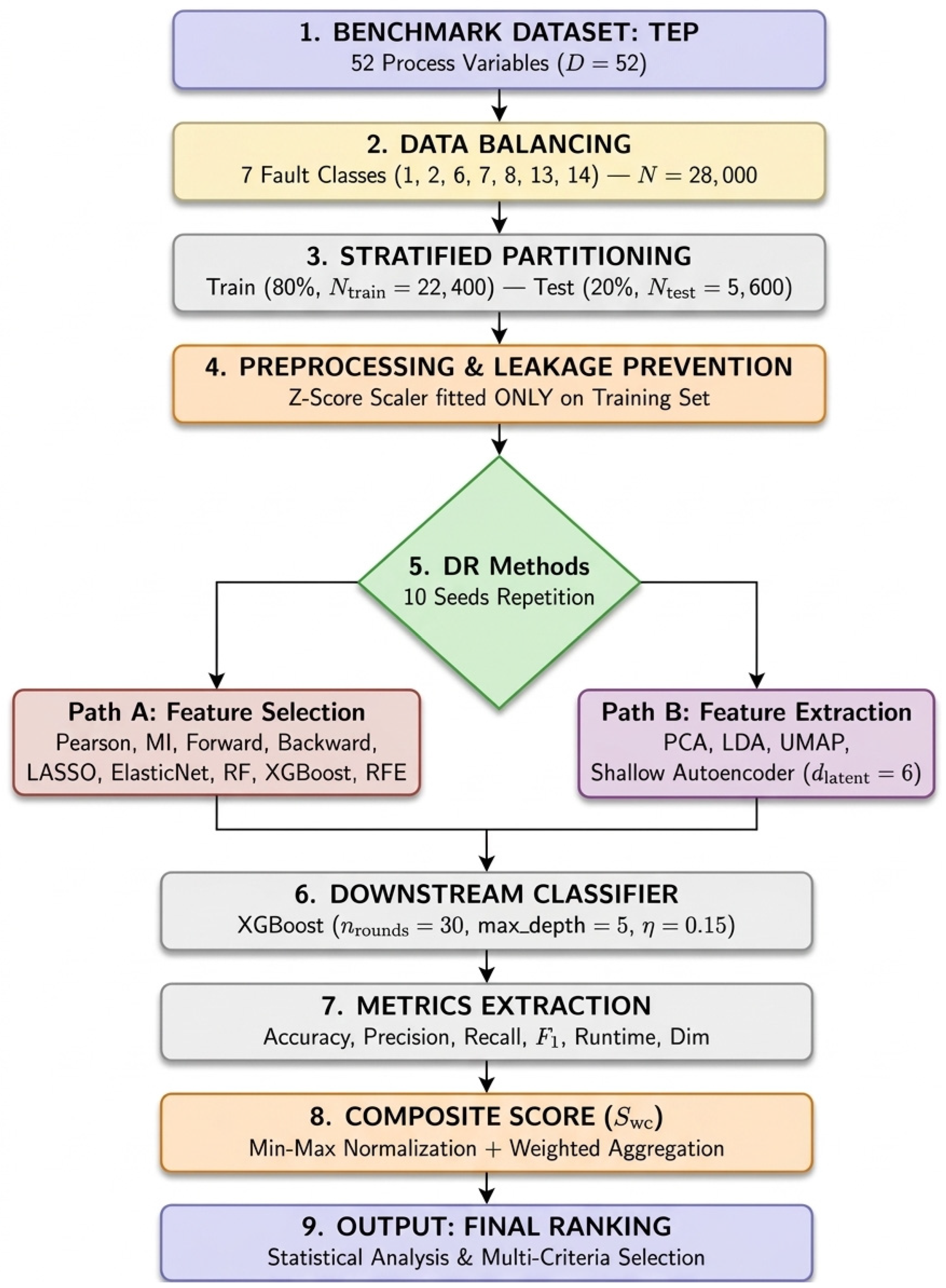
Representation dimensionality was recorded as the number of selected variables for feature selection methods and the number of extracted dimensions for feature extraction methods. These quantities, together with the predictive performance measures and computational time, were subsequently used in the composite score described in Section 3. The overall experimental procedure is summarized in Figure 1. The workflow begins with the balanced TEP dataset and stratified train–test partitioning, followed by training set-based standardization. The resulting data are processed through either the feature selection or feature extraction path. Each resulting representation is then evaluated using the common XGBoost classifier. Predictive performance, computational time, and representation dimensionality are recorded for each repetition. Finally, these quantities are incorporated into the composite scoring framework to obtain method-specific scores and rankings. The repeated experimental design provides a common basis for evaluating the competing dimensionality reduction methods. By maintaining the same data partition strategy, preprocessing procedure, downstream classifier, predictive metrics, and scoring procedure across methods, the comparison focuses on the relative trade-off among predictive performance, computational cost, and representation compactness.

4.3. Baseline Classification Performance

The baseline results indicate that the complete process variable representation provides a strong and stable reference for the classification task. Before evaluating feature selection (FS) and feature extraction (FE) strategies, a baseline experiment was conducted using all 52 process variables. The variables were standardized using the training partition only, and the XGBoost multiclass classifier was evaluated over 10 independently generated stratified train–test partitions. The mean and standard deviation of the obtained metrics are reported in

Table 3. Baseline performance of XGBoost using the complete process variable representation.

Method	Features	Accuracy	Precision	Recall	F1-Score	Time (s)
Baseline XGBoost	52	0.9354 ± 0.0024	0.9456 ± 0.0019	0.9354 ± 0.0024	0.9381 ± 0.0022	12.45 ± 5.53

.

The low standard deviations of the predictive metrics indicate consistent performance across the repeated partitions. This baseline is used as a reference rather than included in the composite ranking, because the proposed criterion is intended to compare alternative FS and FE representations in terms of predictive performance, dimensionality, and computational cost.

4.4. Overall Performance of Feature Selection Methods

The results show that the feature selection methods provide different trade-offs between predictive performance, computational time, and the number of selected features. Pearson correlation achieves the highest predictive performance among the FS methods, with an F1-score of 0.9333 ± 0.0021 using 35 features. Backward elimination also provides competitive predictive accuracy, achieving an F1-score of 0.9266 ± 0.0042 with only 10 selected features.

Table 4. Raw performance of feature selection methods over 10 stratified repetitions.

Method	Accuracy	Precision	Recall	F1-Score	Time (s)	Selected Features
Backward Elimination	0.9233 ± 0.0044	0.9353 ± 0.0045	0.9233 ± 0.0044	0.9266 ± 0.0042	32.54 ± 21.50	10
Elastic Net	0.8270 ± 0.0039	0.8583 ± 0.0031	0.8270 ± 0.0039	0.8313 ± 0.0038	18.21 ± 9.26	14
Forward Selection	0.8874 ± 0.0020	0.9042 ± 0.0020	0.8874 ± 0.0020	0.8893 ± 0.0020	4.44 ± 3.26	10
LASSO	0.8986 ± 0.0189	0.9180 ± 0.0137	0.8986 ± 0.0189	0.9019 ± 0.0179	36.76 ± 19.24	14
Mutual Information	0.8905 ± 0.0026	0.9081 ± 0.0024	0.8905 ± 0.0026	0.8928 ± 0.0026	5.14 ± 3.97	12
Pearson	0.9303 ± 0.0024	0.9412 ± 0.0014	0.9303 ± 0.0024	0.9333 ± 0.0021	9.52 ± 7.15	35
RFE	0.9106 ± 0.0039	0.9244 ± 0.0038	0.9106 ± 0.0039	0.9145 ± 0.0036	46.40 ± 35.34	8
Random Forest	0.9153 ± 0.0061	0.9293 ± 0.0049	0.9153 ± 0.0061	0.9192 ± 0.0056	70.71 ± 27.77	12
XGBoost	0.9153 ± 0.0069	0.9284 ± 0.0066	0.9153 ± 0.0069	0.9189 ± 0.0067	12.63 ± 6.41	9

presents the mean and standard deviation of the raw classification metrics, computational time, and number of selected features obtained over 10 independently generated stratified train–test partitions.

Pearson correlation offers the closest predictive performance to the baseline (0.9381 F1-score) while reducing the feature set from 52 to 35. Conversely, methods such as forward selection and mutual information achieve much lower computational times and moderate feature compression, but with a slight compromise in predictive performance. These clear trade-offs emphasize that evaluating feature selection strategies based solely on classification accuracy is insufficient, thereby justifying the application of the proposed multicriteria composite score (S_wc).

4.5. Overall Performance of Feature Extraction Methods

The results show clear differences among the feature extraction (FE) methods in terms of predictive performance, computational cost, and latent space dimensionality. LDA provides the highest predictive performance among the evaluated FE methods, achieving an F1-score of 0.8874 ± 0.0029 with six dimensions. In contrast, the autoencoder exhibits the lowest predictive accuracy (0.6627 ± 0.0236 F1-score), while UMAP requires substantially higher computational time despite utilizing the same target dimension as LDA (six dimensions).

Table 5. Raw performance of feature extraction methods over 10 stratified repetitions.

Method	Accuracy	Precision	Recall	F1-Score	Time (s)	Dimensions
Autoencoder	0.6664 ± 0.0223	0.6916 ± 0.0223	0.6664 ± 0.0223	0.6627 ± 0.0236	5.71 ± 3.26	6
LDA	0.8836 ± 0.0030	0.9053 ± 0.0023	0.8836 ± 0.0030	0.8874 ± 0.0029	4.08 ± 2.66	6
PCA	0.8290 ± 0.0054	0.8485 ± 0.0049	0.8290 ± 0.0054	0.8306 ± 0.0054	5.58 ± 4.58	14
UMAP	0.7844 ± 0.0149	0.8059 ± 0.0168	0.7844 ± 0.0149	0.7901 ± 0.0154	155.06 ± 71.85	6

presents the mean and standard deviation of the classification metrics, computational time, and reduced dimensions obtained over 10 independently generated stratified train–test partitions.

Among the evaluated FE techniques, LDA yields the highest predictive scores alongside the lowest execution time. PCA achieves intermediate predictive accuracy using a 14-dimensional representation. Although UMAP reduces the feature space to six dimensions, its high computational execution time (155.06 ± 71.85 s) impacts its practical efficiency in this configuration.

4.6. Sensitivity of the Composite Ranking to Weight Selection

To assess the sensitivity of the proposed composite ranking framework, four weighting scenarios were evaluated. These scenarios represent different operational priorities among predictive performance, computational efficiency, and representation dimensionality. The Balanced scenario assigns moderate importance across all criteria, whereas the Predictive Focus scenario places primary emphasis on classification performance. The Efficiency Focus scenario increases the weight assigned to execution time, while the Compactness Focus scenario prioritizes feature space dimensionality reduction.

Table 6. Weighting scenarios used in the sensitivity analysis.

Scenario	wacc	wprec	wrec	WF1	λtime	λdim
Balanced	0.30	0.10	0.10	0.10	0.20	0.20
Predictive Focus	0.35	0.12	0.12	0.11	0.15	0.15
Efficiency Focus	0.25	0.08	0.08	0.09	0.30	0.20
Compactness Focus	0.25	0.08	0.08	0.09	0.15	0.35

summarizes the weighting schemes applied in the sensitivity analysis. The weights are distributed across Accuracy, Precision, Recall, F1-score, computational time, and dimensionality, with the total weight normalized to one for each scenario.

These scenarios provide a controlled basis for examining whether shifts in criteria importance alter the relative ordering of the FS and FE methods. As reported in

Table 7. Scenario-based composite evaluation of feature selection methods.

Scenario	Method	Predictive Component	Time Penalty	Dimension Penalty	Composite Score (Swc)	Rank
Balanced	Forward Selection	0.53431	0.00000	0.01481	0.51950	1
	XGBoost	0.55085	0.02472	0.00741	0.51873	2
	Mutual Information	0.53629	0.00211	0.02963	0.50455	3
	Backward Elimination	0.55551	0.08480	0.01481	0.45589	4
	RFE	0.54813	0.12663	0.00000	0.42150	5
	Elastic Net	0.49976	0.04156	0.04444	0.41376	6
	LASSO	0.54143	0.09754	0.04444	0.39945	7
	Pearson	0.55957	0.01533	0.20000	0.34424	8
	Random Forest	0.55097	0.20000	0.02963	0.32134	9
Predictive Focus	XGBoost	0.64268	0.01854	0.00556	0.61858	1
	Forward Selection	0.62341	0.00000	0.01111	0.61229	2
	Mutual Information	0.62572	0.00158	0.02222	0.60191	3
	Backward Elimination	0.64811	0.06360	0.01111	0.57340	4
	RFE	0.63951	0.09498	0.00000	0.54453	5
	LASSO	0.63171	0.07316	0.03333	0.52522	6
	Elastic Net	0.58313	0.03117	0.03333	0.51863	7
	Pearson	0.65285	0.01150	0.15000	0.49135	8
	Random Forest	0.64282	0.15000	0.02222	0.47060	9
Efficiency Focus	Forward Selection	0.44522	0.00000	0.01481	0.43040	1
	XGBoost	0.45902	0.03708	0.00741	0.41454	2
	Mutual Information	0.44687	0.00317	0.02963	0.41407	3
	Backward Elimination	0.46291	0.12721	0.01481	0.32089	4
	Elastic Net	0.41639	0.06234	0.04444	0.30961	5
	RFE	0.45676	0.18995	0.00000	0.26680	6
	LASSO	0.45115	0.14631	0.04444	0.26039	7
	Pearson	0.46629	0.02300	0.20000	0.24330	8
	Random Forest	0.45912	0.30000	0.02963	0.12949	9
Compactness Focus	XGBoost	0.45902	0.01854	0.01296	0.42752	1
	Forward Selection	0.44522	0.00000	0.02593	0.41929	2
	Mutual Information	0.44687	0.00158	0.05185	0.39343	3
	Backward Elimination	0.46291	0.06360	0.02593	0.37338	4
	RFE	0.45676	0.09498	0.00000	0.36178	5
	Elastic Net	0.41639	0.03117	0.07778	0.30745	6
	LASSO	0.45115	0.07316	0.07778	0.30022	7
	Random Forest	0.45912	0.15000	0.05185	0.25727	8
	Pearson	0.46629	0.01150	0.35000	0.10479	9

Note: The predictive component was calculated from the mean Accuracy, Precision, Recall, and F1-score values reported in the raw performance results using the corresponding scenario-specific weights in Table 6. No additional normalization was applied to these predictive metrics. Computational time and dimensionality were normalized independently for the FS methods using min–max normalization.

, the scenario-based composite scores show that the relative ranking of the leading methods remains stable, although minor positional shifts occur under specific weighting profiles.

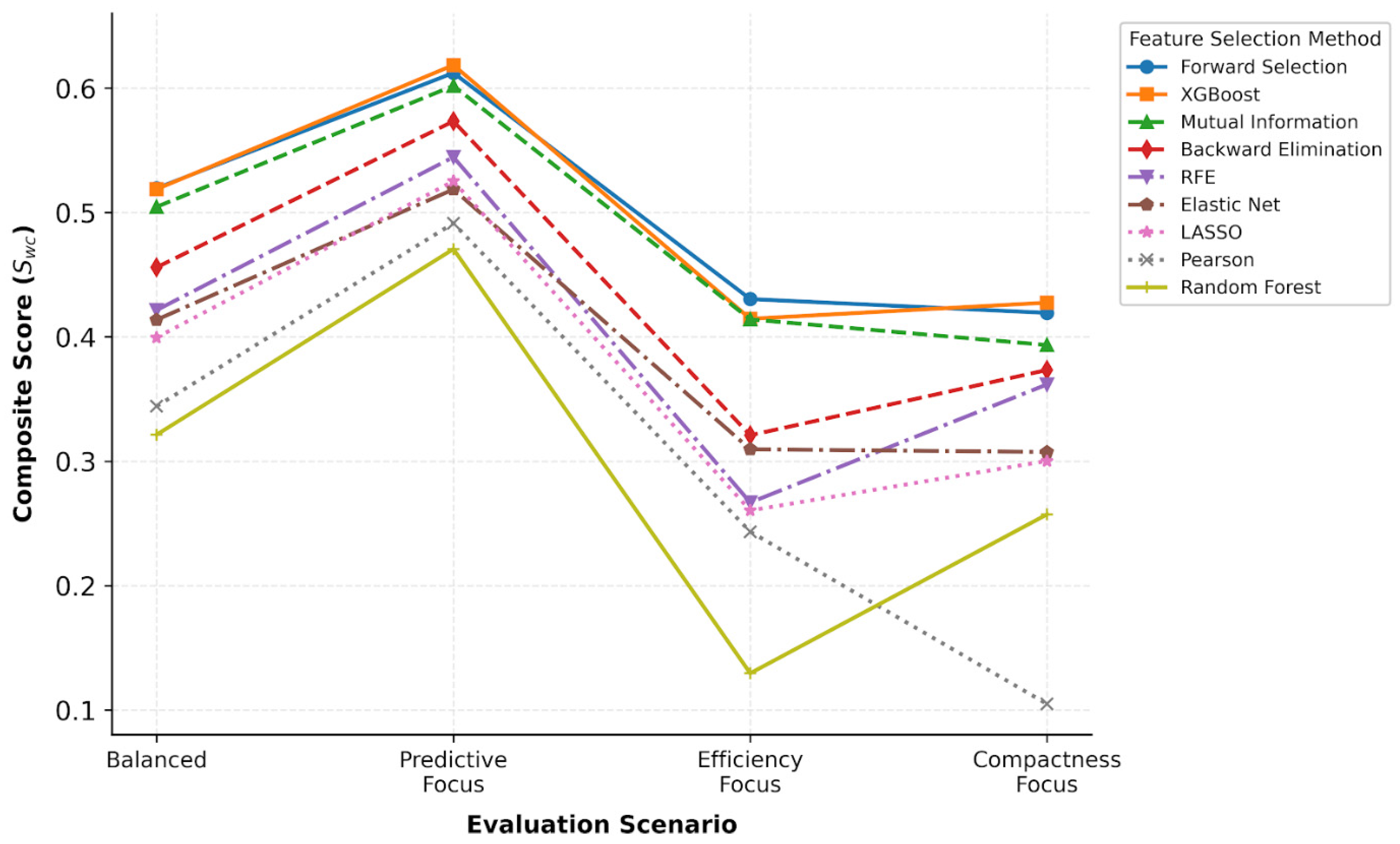
As illustrated in Figure 2, the composite evaluation framework demonstrates consistent ranking stability across varying evaluation priorities, confirming that top-tier methods retain their competitive advantage regardless of moderate weight variations.

The composite evaluation scores (S_wc) presented in Figure 2 illustrate the performance stability and sensitivity of feature selection methods across various evaluation scenarios. Across all scenarios, forward selection, XGBoost, and mutual information consistently demonstrated high performance, forming the top-performing trio. In the “Predictive Focus” scenario, scores for all methods rose to peak levels, with XGBoost achieving the highest value at 0.61858. Conversely, in the “Efficiency Focus” scenario, a marked decline in scores was observed across all methods due to the computational time penalty; here, forward selection (0.43040), characterized by low computational cost, rose to first place. Random forest, which incurred the highest time penalty, dropped to a score of 0.12949, experiencing the sharpest decline in performance. In the “Compactness Focus” scenario, performance patterns shifted as the weight of the dimensionality penalty increased. The Pearson correlation method, which selects a large number of features, fell to last place with a score of 0.10479 due to this penalty. In contrast, methods such as RFE and random forest showed a resurgence in this scenario, benefiting from their ability to select fewer features. Overall, forward selection and XGBoost emerged as the standout methods, maintaining a balanced performance profile across all experimental scenarios.

Following the evaluation of the feature selection methods, the same composite ranking framework was applied to the feature extraction (FE) methods.

Table 8. Scenario-based composite evaluation of feature extraction methods.

Scenario	Method	Predictive Component	Time Penalty	Dimension Penalty	Composite Score (Swc)	Rank
Balanced	LDA	0.53271	0.00000	0.00000	0.53271	1
	Autoencoder	0.40199	0.00216	0.00000	0.39983	2
	PCA	0.49951	0.00199	0.20000	0.29752	3
	UMAP	0.47336	0.20000	0.00000	0.27336	4
Predictive Focus	LDA	0.62154	0.00000	0.00000	0.62154	1
	Autoencoder	0.46910	0.00162	0.00000	0.46748	2
	PCA	0.58282	0.00149	0.15000	0.43133	3
	UMAP	0.55229	0.15000	0.00000	0.40229	4
Efficiency Focus	LDA	0.44388	0.00000	0.00000	0.44388	1
	Autoencoder	0.33488	0.00324	0.00000	0.33164	2
	PCA	0.41620	0.00298	0.20000	0.21322	3
	UMAP	0.39443	0.30000	0.00000	0.09443	4
Compactness Focus	LDA	0.44388	0.00000	0.00000	0.44388	1
	Autoencoder	0.33488	0.00162	0.00000	0.33326	2
	PCA	0.41620	0.00149	0.35000	0.06471	3
	UMAP	0.39443	0.15000	0.00000	0.24443	4

Note: The predictive component was calculated from the mean Accuracy, Precision, Recall, and F1-score values reported in the raw performance results using the corresponding scenario-specific weights in Table 6. No additional normalization was applied to these predictive metrics. Computational time and dimensionality were normalized independently for the FE methods using min–max normalization, where dimensionality represents the extracted latent space size.

presents the resulting performance scores and rank orders across the four weighting scenarios, allowing for an analysis of whether the relative performance order of the FE representations remains stable.

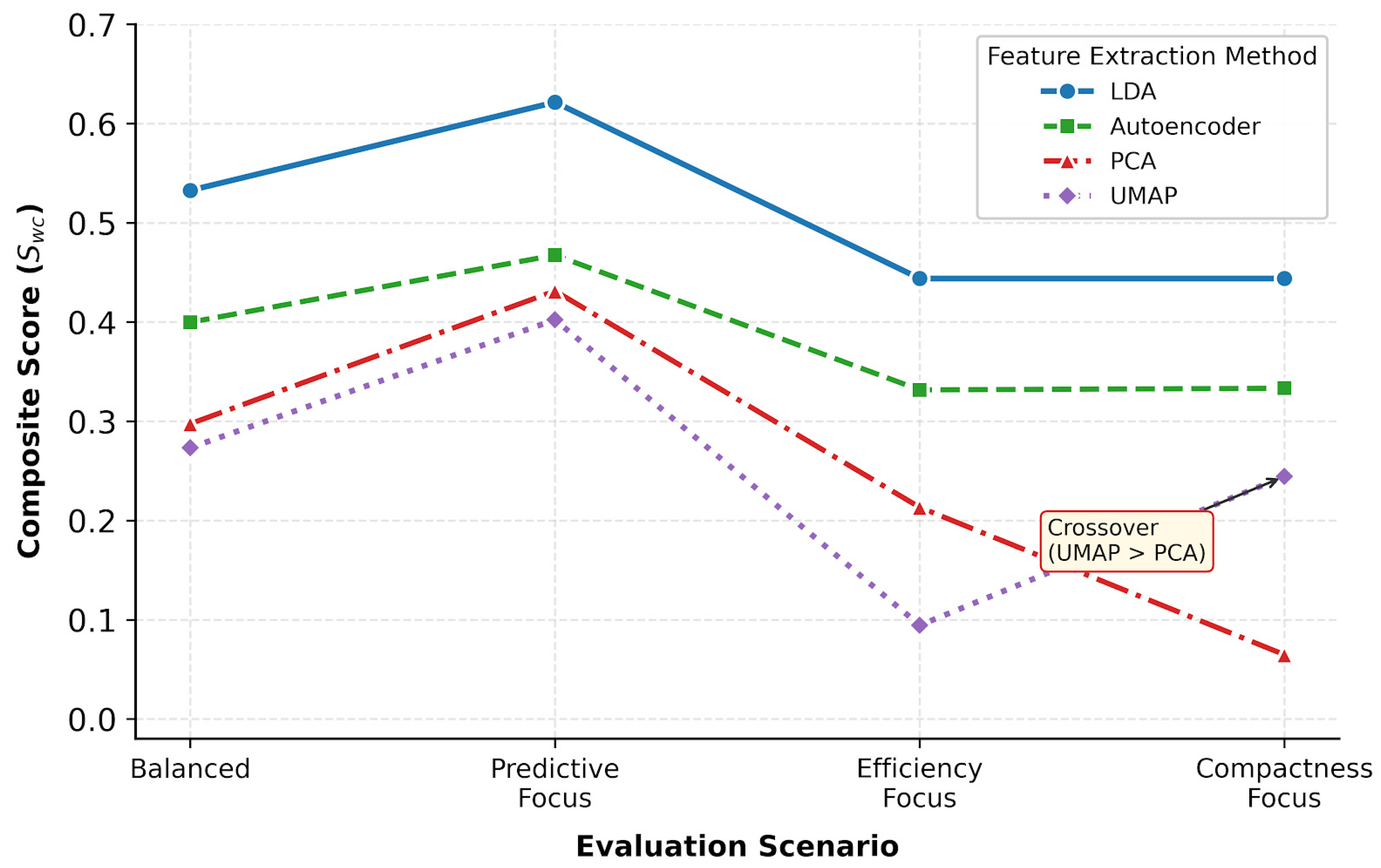
Figure 3 illustrates the trajectory of composite scores (S_wc) across the four weighting scenarios for all evaluated feature extraction methods based on the detailed results in Table 8.

The graphical representation highlights two main trends:

• A dominant performance profile is observed for LDA and autoencoder, which consistently occupy the top two positions across all evaluation profiles. LDA maintains the highest composite score in every scenario (Swc = 0.53271 in Balanced, 0.62154 in Predictive Focus, and 0.44388 in both Efficiency and Compactness Focus) because it combines the highest predictive component with zero time and dimensionality penalties under the evaluated FE methods. Meanwhile, autoencoder follows as a stable runner-up across all four scenarios, with composite scores ranging from 0.33164 to 0.46748. Its consistent second-place ranking is supported by its six-dimensional representation and relatively low computational time, although its predictive performance remains substantially lower than that of LDA.
• Substantial trajectory shifts occur among the lower-ranked methods depending on specific scenario penalties. UMAP experiences a sharp decline under the Efficiency Focus scenario (S_wc = 0.09443) owing to its high execution time penalty (0.30000), whereas PCA suffers its heaviest drop under the Compactness Focus scenario (S_wc = 0.06471) due to its higher feature retention penalty (0.35000). Consequently, a notable rank crossover occurs under the Compactness Focus scenario, where UMAP (S_wc = 0.24443) surpasses PCA to claim the third position.

The trajectories confirm that while supervised and deep learning-based feature extraction methods maintain consistent advantage profiles, unsupervised statistical approaches like PCA and nonlinear embeddings like UMAP exhibit strong sensitivity to operational penalty structures.

To synthesize the sensitivity analysis across all four weighting profiles,

Table 9. Rank stability of FS and FE methods across weighting scenarios.

Group	Method	Mean Rank	SD Rank	Min Rank	Max Rank	IQR Rank
FE	LDA	1.00	0.00	1	1	0.00
FE	Autoencoder	2.00	0.00	2	2	0.00
FE	PCA	3.25	0.50	3	4	0.25
FE	UMAP	3.75	0.50	3	4	0.25
FS	Forward Selection	1.50	0.58	1	2	1.00
FS	XGBoost	1.50	0.58	1	2	1.00
FS	Mutual Information	3.00	0.00	3	3	0.00
FS	Backward Elimination	4.00	0.00	4	4	0.00
FS	RFE	5.25	0.50	5	6	0.25
FS	Elastic Net	6.00	0.82	5	7	0.50
FS	LASSO	6.75	0.50	6	7	0.25
FS	Pearson	8.25	0.50	8	9	0.25
FS	Random Forest	8.75	0.50	8	9	0.25

summarizes the descriptive rank stability statistics for both feature selection (FS) and feature extraction (FE) methods.

The summary statistics in Table 9 indicate a high degree of rank stability across the four weighting scenarios. In the FE group, LDA and autoencoder exhibit complete ranking invariance (SD = 0.00, IQR = 0.00), maintaining ranks 1 and 2 in all four scenarios, respectively. PCA and UMAP show limited positional variation, with each method occupying ranks 3 and 4 across the scenarios (SD = 0.50, IQR = 0.25). In the FS group, mutual information and backward elimination also maintain fixed positions, with mean ranks of 3.00 and 4.00, respectively, and SD = 0.00. Forward selection and XGBoost alternate between ranks 1 and 2, resulting in identical mean ranks of 1.50 (SD = 0.58, IQR = 1.00). The remaining FS methods exhibit relatively limited rank variation, with the largest variability observed for elastic net (SD = 0.82, IQR = 0.50). The rank statistics indicate that the relative ordering of the methods was largely stable across the four weighting scenarios, with variation mainly occurring among methods with closely competing composite scores.

4.7. Statistical Analysis of Method Differences and Ranking Consistency

Nonparametric statistical tests were used to evaluate differences among the feature selection (FS) and feature extraction (FE) methods based on their scenario-level composite scores (S_wc). For each method, Accuracy, Precision, Recall, F1-score, computational time, and representation dimensionality were first obtained from 10 independently generated stratified train–test partitions. The mean value of each metric across the 10 repetitions was then calculated for each method. These mean values were subsequently combined using the four predefined weighting scenarios: Balanced, Predictive Focus, Efficiency Focus, and Compactness Focus to obtain four scenario-specific S_wc values for each method. Thus, the statistical analyses were performed on these four scenario-level S_wc values per method, rather than on the individual observations from the 10 train–test repetitions.

The Friedman test was used to assess whether statistically significant differences existed among the methods within each FS and FE group based on their scenario-level composite scores. Kendall’s W was calculated to quantify the consistency of method rankings across the four weighting scenarios. For post-hoc analysis, paired Wilcoxon signed-rank tests were performed between methods using their four matched scenario-level composite scores, and the resulting p-values were adjusted using the Holm–Bonferroni procedure to account for multiple pairwise comparisons in

Table 10. Overall statistical evaluation and post-hoc comparison of feature selection and feature extraction methods based on scenario-level composite scores (S_wc).

Group	Friedman χ2	df	p-Value	Kendall’s W	Post-Hoc Result (Wilcoxon + Holm)
FS	31.067	8	<0.001	0.971	No individual pair remained significant after Holm correction
FE	11.100	3	0.0112	0.925	No individual pair remained significant after Holm correction

.

The Friedman test indicated statistically significant overall differences among the methods in both groups. For FS, the test yielded χ² (8) = 31.067, p < 0.001, with a Kendall’s W of 0.971. For FE, the corresponding values were χ² (3) = 11.100, p = 0.0112, and Kendall’s W = 0.925. These high Kendall’s W values indicate that the relative ranking of the methods was highly consistent across the four weighting scenarios.

Although the Friedman tests indicated statistically significant overall differences among the methods, none of the individual pairwise comparisons remained statistically significant after Holm–Bonferroni correction. This finding should be interpreted in the context of the statistical unit used in the analysis. The pairwise Wilcoxon tests were based on only four matched scenario-level S_wc observations per method, corresponding to the four weighting scenarios. Therefore, the significant omnibus Friedman results indicate differences in the overall ranking structure among methods, whereas the absence of significant Holm-adjusted pairwise comparisons does not provide sufficient evidence to claim statistically significant superiority of any specific method over another. The observed differences in S_wc and rank should consequently be interpreted as comparative patterns under the predefined weighting scenarios rather than as statistically confirmed pairwise differences. In particular, the leading FS methods, including forward selection, XGBoost, and mutual information, consistently occupied the highest ranks, whereas Pearson correlation and random forest were positioned toward the lower end of the ranking. Similarly, LDA consistently achieved the highest composite score among the FE methods, followed by the autoencoder, whereas PCA and UMAP occupied the lower-ranked positions, with their relative ordering varying under the Compactness Focus scenario.

The results indicate that the weighting profile affected the magnitude of the composite scores but did not substantially alter the relative ranking structure of the methods. The high Kendall’s W values therefore provide evidence of ranking stability across the four evaluation scenarios, whereas the nonsignificant Holm-adjusted pairwise tests indicate that specific pairwise differences should not be interpreted as statistically confirmed.

5. Discussion

The experimental results demonstrate that the evaluation of dimensionality reduction methods depends on the criteria considered during the assessment process. Predictive performance is an important criterion for fault diagnosis, but it does not fully describe the computational and representational characteristics of a method. In the proposed framework, Accuracy, Precision, Recall, F1-score, computational time, and representation dimensionality were obtained from 10 repeated stratified train–test experiments. For each method, the results across the 10 repetitions were first averaged, and these mean values were subsequently used to calculate the weighted composite score (S_wc) under four evaluation scenarios: Balanced, Predictive Focus, Efficiency Focus, and Compactness Focus. The FS and FE methods were evaluated separately using the same procedure. Therefore, the resulting composite scores represent a combined assessment of predictive performance, computational cost, and representation size rather than predictive performance alone.

The sensitivity analysis showed that changing the weighting profile affected the magnitude of the composite scores and, for some methods, their relative positions. Nevertheless, several methods maintained stable ranking profiles across the four scenarios. The statistical analysis was conducted using the four scenario-level composite scores derived from the mean results of the 10 repetitions. The Friedman tests indicated overall differences among the methods in both the FS and FE groups, while the high Kendall’s coefficients of concordance indicated strong consistency of the rankings across the weighting scenarios. However, none of the pairwise Wilcoxon signed-rank comparisons remained statistically significant after Holm correction. Thus, the observed ranking differences should be interpreted as comparative performance patterns under the evaluated weighting profiles rather than as evidence of statistically confirmed pairwise superiority.

5.1. Discussion of Feature Extraction Results

Among the evaluated feature extraction (FE) methods, linear discriminant analysis (LDA) achieved the highest composite score in all four weighting scenarios and maintained rank 1 throughout the sensitivity analysis. Its composite scores were 0.53271, 0.62154, 0.44388, and 0.44388 for the Balanced, Predictive Focus, Efficiency Focus, and Compactness Focus scenarios, respectively. LDA also produced a six-dimensional representation and had the lowest mean computational time among the evaluated FE methods. Its mean F1-score was 0.8874, providing a favorable combination of predictive performance, computational efficiency, and representation compactness. The supervised nature of LDA allows the transformation to incorporate class information, which can be advantageous when the objective is to obtain representations that preserve class-discriminative information.

The autoencoder consistently occupied the second position across all four weighting scenarios. It generated a six-dimensional latent representation and required relatively low computational time. However, its predictive performance was lower than that of LDA, with a mean F1-score of 0.6627 compared with 0.8874 for LDA. Its second position in the composite ranking reflects the combination of its predictive performance with its low computational time and compact six-dimensional representations. The result indicates that the compact latent representation obtained by the autoencoder remained competitive when computational and dimensionality criteria were included in the evaluation. The use of neural networks for learning low-dimensional representations is consistent with the dimensionality reduction approach described by [20].

PCA ranked third under the Balanced, Predictive Focus, and Efficiency Focus scenarios and moved to fourth position under the Compactness Focus scenario. PCA achieved a mean F1-score of 0.8306 using 14 components. Although its predictive performance was higher than that of the autoencoder, its 14-dimensional representation was larger than the six-dimensional representations produced by LDA, autoencoder, and UMAP. Consequently, PCA received a dimensionality penalty that became more influential as greater weight was assigned to representation compactness. This effect was most pronounced under the Compactness Focus scenario, where the dimensionality penalty reached 0.35000, and PCA moved to fourth position. The result is consistent with the fundamental objective of PCA, which constructs components that successively maximize variance rather than directly optimizing class separation [45].

UMAP produced a six-dimensional representation and achieved a mean F1-score of 0.7901. However, its mean computational time was substantially higher than that of the other FE methods, reaching 155.06 s. Consequently, the computational time penalty had a strong effect on its composite score, particularly under the Efficiency Focus scenario, where UMAP obtained a score of 0.09443 and ranked fourth. Under the Compactness Focus scenario, UMAP moved to third position and exceeded PCA because the increased dimensionality weight imposed a larger penalty on PCA’s 14-dimensional representation, whereas UMAP retained a six-dimensional representation and therefore received no dimensionality penalty. These results illustrate how computational cost and representation dimensionality can influence the comparative evaluation of nonlinear dimensionality reduction methods [21].

The FE results indicate that LDA provided the most favorable composite profile under the experimental conditions considered in this study. The stable second position of the autoencoder demonstrates that compact latent representations can remain competitive when computational time and dimensionality are explicitly incorporated into the evaluation. The different positions of PCA and UMAP across the weighting scenarios further show that the preferred method can depend on the relative importance assigned to the evaluation criteria.

5.2. Discussion of Feature Selection Results

The feature selection (FS) results demonstrate more pronounced trade-offs between predictive performance, computational time, and the number of selected variables. This observation is consistent with recent industrial fault classification research emphasizing the potential of feature selection to reduce redundant process variables while maintaining diagnostic performance [46].

Pearson correlation achieved the highest predictive performance among the FS methods, with a mean Accuracy of 0.9303 and a mean F1-score of 0.9333. However, it retained 35 of the original 52 variables, representing the largest feature subset among the evaluated FS methods. Consequently, Pearson received the highest dimensionality penalty in the FS group, which substantially reduced its composite score despite its strong predictive performance. This result demonstrates that the method with the highest predictive performance does not necessarily achieve the highest composite ranking when computational cost and representation dimensionality are considered simultaneously.

Forward selection and XGBoost-based feature selection formed the leading group across the four weighting scenarios. Both methods alternated between the first and second positions, resulting in identical mean ranks of 1.50 (SD = 0.58, IQR = 1.00). Forward selection ranked first under the Balanced and Efficiency Focus scenarios, with composite scores of 0.51950 and 0.43040, respectively. Its relatively low computational time of 4.44 s and 10 selected variables contributed to its favorable composite performance, particularly when greater emphasis was placed on computational efficiency. XGBoost-based selection ranked first under the Predictive Focus and Compactness Focus scenarios, achieving composite scores of 0.61858 and 0.42752, respectively, while retaining nine variables. Its first-place position under the Predictive Focus scenario reflects its stronger predictive component, whereas its nine-variable representation also provided a favorable dimensionality profile. These results indicate that the relative position of forward selection and XGBoost-based selection depended on the weighting assigned to predictive performance, computational time, and dimensionality rather than on predictive performance alone.

Mutual information consistently ranked third across all four scenarios, with a mean rank of 3.00. Its relatively low computational time and moderate feature reduction allowed it to maintain a stable composite profile. Backward elimination also showed complete ranking stability, maintaining fourth position in all scenarios with a mean rank of 4.00. Although backward elimination provided relatively strong predictive performance, its computational time was higher than that of forward selection and mutual information.

RFE selected only eight variables, providing the smallest feature subset among the FS methods. However, its iterative feature elimination procedure resulted in a comparatively high computational time. Therefore, the advantage of its compact representation was partly offset by its computational penalty, resulting in a mean rank of 5.25 across the four scenarios.

Elastic net and LASSO occupied the middle to lower part of the FS ranking. Both methods produced moderate feature subsets, but their predictive and computational profiles resulted in lower composite scores than those of the leading FS methods. Random forest was particularly sensitive to computational weighting because it had the highest mean execution time among the FS methods, at 70.71 s. Its composite score consequently decreased substantially under the Efficiency Focus scenario, reaching 0.12949.

The FS results show that the method providing the highest predictive performance does not necessarily achieve the highest composite score. Pearson correlation illustrates this trade-off because its relatively high predictive performance was accompanied by a substantially larger feature set. In contrast, forward selection and XGBoost-based selection provided more favorable overall profiles by combining competitive predictive performance with smaller feature subsets and lower computational requirements.

5.3. Importance of Multicriteria Evaluation in Industrial Applications

Modern industrial machine learning systems must often satisfy several operational requirements simultaneously. Recent studies in smart manufacturing and industrial fault diagnosis have emphasized the importance of considering predictive performance together with computational complexity, scalability, memory requirements, and latency [47,48,49]. While diagnostic reliability remains important, computational requirements and representation size can also influence the feasibility of practical deployment, particularly in resource-constrained environments.

The proposed framework evaluates dimensionality reduction methods using predictive performance, computational time, and representation dimensionality within a weighted composite score. Different weighting scenarios allow the relative importance of these criteria to be assessed under alternative evaluation priorities.

The results illustrate these trade-offs. Pearson correlation achieved high predictive performance but retained 35 variables, whereas UMAP required substantially higher computational time despite producing a six-dimensional representation. In contrast, forward selection, XGBoost-based selection, and LDA achieved higher composite rankings by providing more balanced profiles across the evaluated criteria.

The sensitivity analysis showed that moderate changes in the weighting priorities did not substantially alter the ranking structure of the leading methods. LDA and autoencoder maintained the first and second positions across all FE scenarios, while forward selection, XGBoost-based selection, and mutual information remained the leading FS methods. This ranking stability is supported by the high Kendall’s W values for FS (W = 0.971) and FE (W = 0.925).

The Friedman tests indicated significant overall differences among the methods in both groups. However, no individual pairwise comparison remained significant after Holm correction. Thus, the results support strong consistency in the overall ranking structure but do not establish statistically significant pairwise superiority between individual methods.

5.4. Practical Implications

The proposed framework provides a structured comparison of dimensionality reduction methods when predictive performance, computational cost, and representation size must be considered simultaneously. This is particularly useful when methods provide similar predictive performance but differ in computational requirements or dimensionality.

Feature selection and feature extraction also involve different practical considerations [46]. Feature selection preserves the original process variables, which can facilitate physical interpretation and sensor-level traceability. Feature extraction instead transforms the original variables into a latent representation. Although this can provide substantial dimensional compression, the resulting components generally have less direct correspondence with individual physical process variables.

Under the experimental conditions considered in this study, LDA provided the highest composite ranking among the FE methods, whereas forward selection and XGBoost-based selection formed the leading FS group. These results represent the comparative behavior of the evaluated methods for the selected TEP fault classes, experimental settings, downstream XGBoost classifier, and weighting configurations, rather than universal rankings.

An important practical advantage of the proposed framework is its flexibility. The relative importance assigned to predictive performance, computational time, and dimensionality can be modified according to the intended application. For example, greater emphasis on computational time may be appropriate for resource-constrained or near real-time monitoring, whereas greater emphasis on predictive performance may be appropriate for applications where classification accuracy is the primary concern. The same evaluation framework can therefore be adapted without changing the underlying experimental procedure.

5.5. Limitations and Future Research Directions

Several limitations should be considered when interpreting the findings of this study.

• Dataset Scope: The evaluation was conducted using selected fault classes from the Tennessee Eastman Process (TEP) benchmark. Additional industrial and real-world datasets should be evaluated to assess the generalizability of the proposed framework [48,49].
• Classifier Dependency: XGBoost was used as the common downstream classifier to maintain a controlled comparison among the dimensionality reduction methods. However, the interaction between dimensionality reduction techniques and the downstream learning algorithm may affect the resulting predictive performance and composite scores. Future studies should therefore examine alternative classifiers, including neural networks, support vector machines, and other gradient boosting approaches.
• Weight Determination: The composite score depends on predefined weighting scenarios. Although the present study examined Balanced, Predictive Focus, Efficiency Focus, and Compactness Focus scenarios, alternative weighting strategies may produce different composite scores and rankings. Future research could investigate data-driven or adaptive weighting approaches, including multicriteria decision-making methods such as AHP and TOPSIS.
• Statistical Evaluation: The statistical analysis was performed using four scenario-level composite scores calculated from the mean results of the 10 repeated experiments. This approach was used to evaluate the consistency of method rankings across the predefined weighting profiles. The Friedman tests indicated significant overall differences for both FS and FE, and the high Kendall’s W values indicated strong ranking agreement. However, the limited number of scenario-level observations restricted the resolution of pairwise statistical comparisons. None of the pairwise Wilcoxon signed-rank comparisons remained significant after Holm correction. Future research could examine a larger number of weighting scenarios to provide a more detailed assessment of ranking differences.
• Expanded Evaluation Criteria: The current framework incorporates predictive performance, computational time, and representation dimensionality. Future extensions could include additional deployment-related criteria such as memory usage, energy consumption, inference latency, interpretability, and robustness to noise. These criteria may provide further information for evaluating dimensionality reduction methods in practical industrial environments.

6. Conclusions

This study proposed a weighted composite evaluation framework for comparing feature selection (FS) and feature extraction (FE) methods in industrial fault diagnosis. The framework combines predictive performance, computational time, and representation dimensionality into a single composite score. For each method, the evaluation criteria obtained from 10 repeated stratified train–test experiments were first averaged. These mean values were then used to calculate weighted composite scores under four evaluation scenarios: Balanced, Predictive Focus, Efficiency Focus, and Compactness Focus. The same procedure was applied separately to the FS and FE groups.

The experimental results on the Tennessee Eastman Process dataset showed clear differences in the trade-offs among predictive performance, computational cost, and representation size. Within the FE group, LDA achieved the highest composite score in all four weighting scenarios and maintained rank 1 throughout the sensitivity analysis. The autoencoder consistently ranked second, while PCA and UMAP occupied the third and fourth positions, with their relative ordering changing under the Compactness Focus scenario.

Within the FS group, forward selection and XGBoost-based feature selection showed the most stable high-ranking profiles. Both methods alternated between the first and second positions across the four weighting scenarios, resulting in an identical mean rank of 1.50. Mutual information consistently ranked third. Pearson correlation achieved relatively high predictive performance but was penalized by its larger retained feature set, while random forest was more strongly affected by its computational time.

The statistical analysis was conducted using the scenario-level composite scores derived from the mean results of the 10 repetitions. The Friedman test indicated overall differences among the methods in both the FS and FE groups, with χ² (8) = 31.067, p < 0.001 for FS and χ² (3) = 11.100, p = 0.0112 for FE. Kendall’s coefficients of concordance were high for both groups (W = 0.971 for FS and W = 0.925 for FE), indicating strong consistency in the method rankings across the four weighting scenarios. However, none of the individual pairwise Wilcoxon signed-rank comparisons remained statistically significant after Holm correction. Therefore, the results support stable differences in the overall ranking structure, but they do not provide statistical evidence of pairwise superiority between specific methods after multiple comparison adjustment.

The findings demonstrate that evaluating dimensionality reduction methods using predictive performance alone may not reflect their computational and representational characteristics. The proposed composite framework provides a simple way to incorporate these criteria and examine how method rankings change according to different evaluation priorities. The results are specific to the selected TEP fault classes, experimental settings, downstream XGBoost classifier, and weighting configurations. Future studies can extend the framework to additional industrial datasets, alternative classifiers, adaptive weighting approaches, and deployment-related criteria such as memory usage and energy consumption.