Article

Joint Posterior Reachable-Region Prediction via Local Markov Factor Graphs

1
School of Astronautics, Harbin Institute of Technology, Harbin 150001, China
2
Xi’an Modern Control Technology Research Institute, Xi’an 710065, China
*
Author to whom correspondence should be addressed.
Mathematics 2026, 14(18), 3383; https://doi.org/10.3390/math14183383 (registering DOI)
Submission received: 13 August 2026 / Revised: 8 September 2026 / Accepted: 10 September 2026 / Published: 17 September 2026
(This article belongs to the Section D1: Probability and Statistics)

Abstract

Predicting the future occupied regions of non-cooperative space objects is critical for close-range situational awareness, on-orbit servicing, and collision risk assessment. Yet, conventional target-wise estimators discard the cross-target uncertainty correlations induced by a shared chaser state, whereas reachable-set propagation methods often prescribe disturbance bounds independent of current observations. With known target identities, this paper presents a joint multi-target state estimation and probabilistic reachable-region prediction method based on a local Markov factor graph. The graph unifies chaser and target states, relative-position measurements, equivalent maneuver variables, and history-supported behavior and pair-interaction factors. Schur complement analysis demonstrates how marginalizing the shared chaser state induces cross-target covariance and transfers information through common observations. The finite-graph posterior is then mapped to a corrected-dynamics inferred-control (CDIC) framework to produce target- and time-indexed probabilistic position regions for evaluating orbital safety. Monte Carlo simulations with common random numbers demonstrate that the joint formulation falls back to independent target estimation when relation evidence is absent, while persistent shared evidence improves prediction-center accuracy and empirical trajectory containment. Parameter-sensitivity and randomized-configuration tests delimit this evidence-conditioned benefit. These findings identify the operating regime where cross-target information improves multi-object state estimation, equivalent-maneuver inference, and probabilistic reachable set prediction.

1. Introduction

Spacecraft close-proximity operations are fundamental to on-orbit servicing, debris removal, and space situational awareness. In non-cooperative cases, however, targets do not provide navigation messages, cooperative markers, or an affirmed maneuver plan. The chaser must infer both the present state and the future occupied region of each target from relative measurements. When several known targets are observed from one uncertain chaser, their likelihoods share the chaser state. Target-wise estimation removes this dependence before prediction and therefore cannot, in general, reproduce the target marginals or cross-covariances of the joint posterior.
Clohessy and Wiltshire established the classical linearized relative-motion dynamics for nearly circular reference orbits, and Yamanaka and Ankersen extended transition modeling to arbitrary elliptical reference orbits [1,2]. At the same time, factor graphs provide a sparse probabilistic modeling tool capable of combining dynamics, measurements, priors, and local constraints within a single graphical architecture [3]. Bayes-tree methods preserve this sparsity during incremental inference [4], while exactly sparse Gaussian process regression and simultaneous trajectory estimation and planning connect historical estimation with future transitions [5,6,7]. For multi-object region prediction, direct target-pair information must nevertheless be distinguished from dependence induced by eliminating a shared state, and the conditions under which the joint posterior reduces to target-wise form must be stated explicitly.
Recent studies have increasingly treated the motion of non-cooperative space objects as a behavior- or intention-recognition problem rather than as purely kinematic extrapolation. Recurrent, attention-based, and transformer models extract intention from noisy, incomplete, or constrained time series [8,9,10,11,12], while strategy and maneuver-intention predictors infer parameters or possible future states for pursuit–evasion and proximity operations [13,14]. These studies confirm that finite histories contain information about latent motion tendencies. Most such models nevertheless output a discrete label, a strategy class, or a learned future trajectory, rather than a target-matched probabilistic occupied region with an interpretable relationship to measurement uncertainty, maneuver capability, and prediction horizon. This gap motivates the use of latent equivalent maneuvers and local Markov coupling to construct continuous probabilistic reachable regions from online measurements.
Reachability analysis provides the complementary set-valued machinery. Ellipsoidal and polyhedral approximations characterize spacecraft states attainable under energy-limited or bounded control [15,16], whereas uncertain initial states and process noise generate three-dimensional relative reachable domains [17,18,19]. Ellipsotopes generalize several convex-set representations while retaining linear-map and Minkowski-sum operations [20]. These results also show why a posterior probability region, an independently specified residual support, and a deterministic physical dilation must be treated as distinct sets. Combining them requires an explicit predictive probability measure and a set-inclusion argument.
The reviewed methods fall into two broad classes. State- or set-estimation methods export target-wise posteriors after removing dependence induced by the shared observer state, whereas reachable-set and chance-constrained methods generally prescribe a disturbance model or prediction distribution. The proposed finite-history local Markov factor graph combines both classes through a shared chaser chain, augmented target states, latent equivalent maneuvers, and history-supported target-pair factors. Eliminating the shared block from the sparse MAP information system produces an explicit Schur complement for the target information matrix and vector. The Schur-complement analysis separates direct pairwise information from shared-state-induced information, propagates the associated covariance blocks through the relative-motion dynamics, and characterizes the vanishing-coupling limit. The posterior moments are subsequently mapped into a corrected-dynamics inferred-control (CDIC) construction containing a target-wise posterior region, residual maneuver support, deterministic dilation, and a time-indexed tube. A dependence-free probability bound and a support-function construction complete the set-valued interpretation.
The proposed inference layer is termed space-object inference and reachability (SOIR). SOIR produces target- and time-indexed probabilistic reachable sets for downstream collision-risk assessment rather than performing data association or closed-loop guidance. Multi-object Monte Carlo simulations evaluate the regions under weak, partial, persistent, and signed relations, randomized configurations, and correlated-future stress conditions. Section 2 formulates the joint estimation and reachability model, Section 3 presents the numerical evaluation, and Section 4 summarizes the principal findings, applicability, and limitations.

2. Materials and Methods

2.1. Problem Formulation

2.1.1. Notation and Scenario Geometry

The multi-target scenario is a close-proximity observation problem described in the local orbital frame O . At the current update epoch t i , the chaser state is denoted by x i A , and the augmented state of target B j is denoted by y i B j , j = 1 , , N B , with  N B 2 in the coupled formulation. The supplied relative measurement z i , j couples the shared chaser state and each target state through their relative translational geometry.
Let Δ t be the uniform propagation interval. The finite history contains L h transition intervals and, thus, L h + 1 state epochs, indexed by i L h : i . Meanwhile, the future prediction contains L p transition intervals. Their durations are T h = L h Δ t and T p = L p Δ t . The shorter integer lengths L b and L c specify the behavior-evidence and coupling-score histories, respectively. Let n η be the dimension of the equivalent maneuver state. The required position-selection matrices are defined as follows:
S ρ x = I 3 0 3 × 3 , S ρ y = S ρ x 0 3 × n η ,
so that ρ k A = S ρ x x k A and ρ k B j = S ρ y y k B j .

2.1.2. Chaser Dynamics

The local orbital transition matrices are derived from a standard relative motion model or numerical state-transition propagation. Known deterministic perturbations are included to construct the transition matrices, while unresolved model error is represented by the process covariance [1,2,21,22,23,24].
The physical state of object q { A , B 1 , , B N B } is represented by the following:
x k q = ( ρ k q ) T ( v k q ) T T R 6 , v k q = ρ ˙ k q .
The known control input drives the chaser transition, which is expressed as follows:
x k + 1 A = F k A x k A + G k A u k A + ω k A , ω k A N ( 0 , Q k A , d ) .
The control u k A is a known conditional input not included in the active optimization variables.

2.1.3. Augmented Target State

For target B j , j = 1 , , N B , the physical state with the equivalent maneuver is augmented as follows:
y k B j = ( x k B j ) T ( η k B j ) T T , x k B j = ( ρ k B j ) T ( v k B j ) T T .
The equivalent acceleration η k B j represents a small unmodeled thrust, a behavior-induced perturbation, or a short-term maneuver tendency. The physical state and maneuver then evolve according to
x k + 1 B j = F k B j x k B j + G k B j η k B j + ς k , j B , ς k , j B N ( 0 , Q k , j B , d ) ,
η k + 1 B j = κ η η k B j + ν k , j η , ν k , j η N 0 , Q k , j η ( e ˜ j , k ) , 0 κ η < 1 , Q k , j η ( ϵ ) = Q η , 0 GM + ϵ Q η , ev GM , ϵ [ 0 , 1 ] .
The coefficient κ η denotes the discrete persistence of the latent equivalent-maneuver conditional mean. A continuous-time Gauss–Markov parameterization could impose κ η = exp ( Δ t / τ ) for a generic time constant τ > 0 , whereas Equation (6) requires only 0 κ η < 1 . The numerical implementation calibrates conditional-mean persistence independently of the auxiliary, history-calibrated forecast-covariance memory reported in Section 3. The covariance-memory law does not determine the latent conditional mean. Matrix Q η , 0 GM S + + n η represents the nominal maneuver-innovation covariance, and  Q η , ev GM S + n η represents the event-dependent relaxation increment. ϵ serves as a generic event-intensity argument of Q k , j η ( ϵ ) . The soft box penalty estimates the event state, and the interval-clipping operator clip [ 0 , 1 ] ( a ) : = min { 1 , max { 0 , a } } supplies the raw event refresh. At outer iteration r, the covariance argument e ˜ j , k ( r ) is held fixed during the inner solve. The raw event refresh is clip [ 0 , 1 ] ( e ^ j , k ( r ) ) , whereas the next covariance argument is obtained by the under-relaxed update in Equation (32c). The initial argument is set from the entry prior. This bounded covariance argument introduces neither an additional factor nor a MAP residual. Proper boundary information and Levenberg–Marquardt damping stabilize the inner numerical solve [25,26]; the reported posterior covariance is nevertheless formed from the final undamped information matrix.
Stacking Equations (5) and (6) yields the augmented form
y k + 1 B j = A k η , j y k B j + υ k , j y , A k η , j = F k B j G k B j 0 n η × 6 κ η I n η ,
υ k , j y = ( ς k , j B ) T ( ν k , j η ) T T , υ k , j y N ( 0 , Q k , j y ) , Q k , j y = Q k , j y ( e ˜ j , k ) , Q k , j y ( ϵ ) = Q k , j B , d 0 6 × n η 0 n η × 6 Q k , j η ( ϵ ) .

2.1.4. Relative Measurement

The estimator accepts time-stamped three-dimensional relative-position measurements in the local orbital frame. Sensor calibration, frame conversion, and any front-end measurement reconstruction are completed upstream and are therefore outside the factor-graph state and the present derivation. All subsequent factors use the following measurement equation:
z k , j = h k , j x k A , y k B j + ε k , j z , h k , j x k A , y k B j = S ρ y y k B j S ρ x x k A , ε k , j z N ( 0 , R k , j e ) , R k , j e S + + 3 .
Here, z k , j R 3 is the supplied measurement, h k , j ( · ) denotes the measurement function, and  R k , j e is the associated effective covariance. Define n z : = dim ( z k , j ) = 3 for the relative-position interface used here. Retaining n z in the normalized innovation and probability expressions below makes their dependence on measurement dimension explicit. Let C k , j denote the conditioning information available at or before measurement epoch t k . The measurement interface is specified by the conditional moment relations
E ε k , j z C k , j = 0 , R k , j e : = Cov ε k , j z C k , j = E ε k , j z ( ε k , j z ) T C k , j 0 .
The conditional-moment definition introduces anisotropic and time-varying uncertainty without adding a sensor-level parameterization to the factor graph. The pair ( z k , j , R k , j e ) is supplied to SOIR and held fixed during one posterior solve. The measurement–covariance pair is specified independently of future truth, scenario labels, and coverage outcomes. Historical innovations enter only the event-intensity estimate and associated maneuver-process covariance update. Historical innovations neither replace nor rescale the supplied measurement covariance.

2.1.5. Prediction-Feasibility Conditions

The measurement interface in Equation (9) is conditioned on valid upstream measurements and a positive-definite effective covariance. The common-translation gauge of the relative measurements is fixed by the proper chaser-navigation prior at the history-window boundary. The reachable region is constructed only after the finite-graph solve converges and the selected target-position marginals pass the finite-value, symmetry, and positive-definiteness checks described below. These checks establish the numerical admissibility of the local conditional prediction at the current forecast origin; they do not imply global nonlinear observability, physical identifiability of every auxiliary variable, or uniqueness of the nonlinear MAP solution.

2.2. Local Markov Factor Graph

The posterior distribution is represented by sparse local factors associated with the boundary prior, orbital dynamics, measurement likelihood, behavior and equivalent-maneuver evidence, and evidence-supported historical cross-target relations. The local-factor representation follows the standard factor-graph smoothing paradigm in which the global posterior is decomposed into functions involving only the incident variables. The dynamic and measurement factors represent state-space priors and measurement likelihoods, respectively, while the relative-motion transition factors preserve local temporal dependencies. The Gauss–Markov equivalent-maneuver factor is consistent with established maneuvering-target models. The event state modifies the target-local maneuver process without introducing an additional physical motion model [3,4,25,26,27,28,29].
Each Gaussian residual factor follows the common convention
ϕ ζ ( Θ ζ ) exp 1 2 r ζ ( Θ ζ ) Ω ζ 2 , r Ω 2 = r T Ω r ,
where Ω ζ and Θ ζ are the factor information matrix and local scope, respectively. The residual and information matrix specified for each factor below therefore define its Gaussian contribution without repeating Equation (11).

2.2.1. Active Variables

In the transition-only interface, the graph at t i contains only measured-history and current-epoch variables:
Θ i a = { x i L h : i A , y i L h : i B 1 , , y i L h : i B N B , m 1 : N B , i L h : i b , e 1 : N B , i L h : i } .
The vector m j , k b R n η denotes a dynamically regularized behavior–maneuver summary state, and  e j , k R denotes an unconstrained optimization coordinate for a target-wise soft event/change-point intensity. The corresponding soft-limit residual attracts e j , k toward [ 0 , 1 ] , whereas only the bounded outer-configuration value e ˜ j , k [ 0 , 1 ] enters the covariance function. The associated entry priors and temporal factors are defined below.
In the transition-only interface, the future target variables y ˇ i + 1 : i + L p B j are not MAP variables in Equation (12). The solved current joint posterior is propagated with the augmented orbital transition model and process covariance already used by the target dynamics. The future construction therefore requires neither a fitted CV, CA, or CT reference state nor a kinematic reference trajectory or future-truth information.

2.2.2. Equivalent Maneuver Residual Group

The chaser and target dynamic residuals are based on the same transitions as Equations (3) and (5):
r k A , d = x k + 1 A F k A x k A G k A u k A ,
r k , j B , d = x k + 1 B j F k B j x k B j G k B j η k B j .
Factors ϕ k A , d and ϕ k , j B , d follow the formulation in Equation (11), with information matrices ( Q k A , d ) 1 and ( Q k , j B , d ) 1 , respectively. The equivalent maneuver factor consists of a Gauss–Markov innovation term, an energy regularization term, and a componentwise squared limit penalty:
r k , j η GM = η k + 1 B j κ η η k B j , r k , j η E = η k B j , [ r k , j η ] a = max 0 , | [ η k B j ] a | η ¯ j , a , a = 1 , , n η .
Here, η ¯ j = [ η ¯ j , 1 , , η ¯ j , n η ] T denotes the per-axis acceleration bounds, while Q η E , Q η S + + n η represent the energy and soft-limit covariance parameters. Any scalar weighting coefficients are absorbed into these covariance terms, thereby avoiding redundant weight-covariance parameterization. The innovation covariance is identical to the event-dependent covariance Q k , j η ( e ˜ j , k ) defined in Equation (6) and remains constant during each inner least-squares solve.
Substituting these residual terms into the Gaussian factor formulation yields the following:
ϕ k , j η exp { 1 2 [ r k , j η GM [ Q k , j η ( e ˜ j , k ) ] 1 2 + r k , j η E Q η E 1 2 + r k , j η Q η 1 2 ] } .
The event-intensity value fixed during the inner iteration satisfies 0 e ˜ j , k 1 .
The event intensity influences only the Gauss–Markov innovation covariance and remains constant throughout an inner iteration. The limit term is implemented as a soft componentwise squared penalty aligned with the per-axis bounds used in the simulation settings. The limit term is not a hard feasibility constraint.

2.2.3. Gaussian Measurement Residuals

For the relative-position likelihood in Equation (9), the three-dimensional residual is constructed as follows:
r k , j z = z k , j h k , j x k A , y k B j .
Each residual component is expressed in meters. The same positive-definite R k , j e and the corresponding three-dimensional whitened residual are used consistently in the measurement factor, MAP objective, event evidence calculation, and local covariance computation. The quadratic factor below represents the standard whitened Gaussian likelihood formulation used in statistical orbit determination, nonlinear state estimation, and factor graph smoothing [4,26,27,30].
Whitening the residual using R k , j e leads to the squared Mahalanobis energy:
s k , j z = ( r k , j z ) T ( R k , j e ) 1 r k , j z .
The reported factor ϕ k , j z follows Equation (11) with Ω k , j z = ( R k , j e ) 1 . Thus, the likelihood model, linearized information system, and reported covariance are all based on the same Gaussian information matrix.

2.2.4. Behavior and Event Factors

Let k 0 = i L h denote the first active epoch, and let L b be the order of the behavior-evidence history. Define nonnegative weights β such that = 0 L b β = 1 . Let the configured entry prior provide the initial mean and covariance ( m ¯ j , k 0 b , , P m , j , k 0 ) . Matrix F m R n η × n η represents the behavior-state transition matrix, while Q m , Q b S + + n η denote the transition and maneuver-history evidence covariances.
The behavior residuals are introduced as follows:
r j , k 0 b , 0 = m j , k 0 b m ¯ j , k 0 b , , r k , j b , d = m j , k b F m m j , k 1 b , r k , j b , η = m j , k b = 0 L b β η k B j .
The factors ϕ j b , 0 , ϕ k , j b , d , and  ϕ k , j b , η use the three residuals defined in Equation (19) and the corresponding information matrices ( P m , j , k 0 ) 1 , Q m 1 , and  Q b 1 , respectively, following the convention of Equation (11). Consequently, m j , k b cannot be selected independently at every epoch. Instead, it must satisfy the prior/transition constraints while simultaneously explaining the recent equivalent maneuver history. For every batch solve, ϕ j b , 0 is absorbed once into the configured boundary potential Ψ i entry and is not multiplied as an additional factor.
The posterior behavior state enters the pairwise residual below, allowing the behavior factor to contribute information to η and the coupled target posterior. The event variable serves as a target-wise soft change-point coordinate e j , k R whose covariance argument is restricted to [ 0 , 1 ] . At each outer relinearization, the measurement energy s k , j z from Equation (18) and the normalized maneuver-innovation score are evaluated and held fixed as follows:
s k , j η = ( r k 1 , j η GM ) T ( Q η , 0 GM ) 1 r k 1 , j η GM , ν j , k = 1 2 s k , j z / n z + s k , j η / n η , e ¯ j , k = sigm g e ( ν j , k θ e ) , sigm ( a ) : = 1 + exp ( a ) 1 .
Here, ν j , k denotes the dimension-normalized mean of the measurement and maneuver-innovation energies, g e > 0 is the fixed logistic gain, and  θ e > 0 represents the normalized event threshold. Residual r k 1 , j η GM is defined in Equation (15), with  Q η , 0 GM S + + n η being the nominal covariance. The evaluated event-evidence quantities remain fixed during each inner nonlinear solve.
The event state is constrained through temporal, evidence, and box-limit residuals:
r k , j e , d = e j , k κ e e j , k 1 , r k , j e , z = e j , k e ¯ j , k , r k , j e , l i m = max ( 0 , e j , k ) max ( 0 , e j , k 1 ) , ϕ k , j e exp 1 2 r k , j e , d r k , j e , z r k , j e , l i m Q e 1 2 .
0 κ e < 1 is the event-state persistence coefficient, while Q e S + + 4 weights the scalar transition residual, scalar evidence residual, and two box-limit residuals.
At the first active epoch, κ e e j , k 1 is replaced by the configured event-prior mean. Holding ( s k , j z , s k , j η ) constant within an inner Gauss–Newton/LM solve prevents repeated differentiation through the same measurement residual. Both energy quantities are refreshed at the next outer iteration or forecast-origin batch solve.
A high event intensity relaxes the Gauss–Markov maneuver-innovation covariance through the covariance definition in Equation (6) and the corresponding factor realization in Equation (16), thus facilitating abrupt but measurement-supported maneuver changes without converting the event variable into an unconstrained switch.

2.2.5. Correlation Matrix and Coupling Weights

The evidence-supported information exchange between target chains is encoded through the sparse coupling coefficient matrix.
K i c = [ κ j l , i ] N B × N B , κ j j , i = 0 , 0 κ j l , i = κ l j , i 1 .
The matrix entries are weak data-dependent weights computed before the inner solve based on history-only fits and the measurement geometry available at the current forecast origin. In the notation below, ρ ^ j , k h , v ^ j , k h , and  η ^ j , k h are the position, velocity, and maneuver subblocks of the measurement-conditioned target history estimate. The index k = i denotes the corresponding values at the current forecast origin. The vector m ^ j , k b , h is the associated behavior-state history estimate. All four history estimates depend only on the entry information and measurements in Z 0 : i , remain fixed before active pair factors are assembled, and are not additional MAP variables. A representative score combining the four sources is
κ ˜ j l , i = w ρ exp ρ ^ j , i h ρ ^ l , i h 2 2 2 σ ρ 2 + w v exp v ^ j , i h v ^ l , i h 2 2 2 σ v 2 + w exp ^ j , i h ^ l , i h 2 2 2 σ 2 + w η exp η j , i h , avg η l , i h , avg 2 2 2 σ η 2 ,
The score weights satisfy w ρ , w v , w , w η 0 and w ρ + w v + w + w η = 1 , while σ ρ , σ v , σ , σ η > 0 represent the fixed normalization scales.
With the measurement-derived direction ^ j , i h = z i , j / z i , j 2 and the previously defined averaging length L c , the history-averaged maneuver is
η j , i h , avg = 1 L c + 1 s = i L c i η ^ j , s h .
κ j l , i = min ( 1 , κ ˜ j l , i ) , κ ˜ j l , i κ min , 0 , κ ˜ j l , i < κ min .
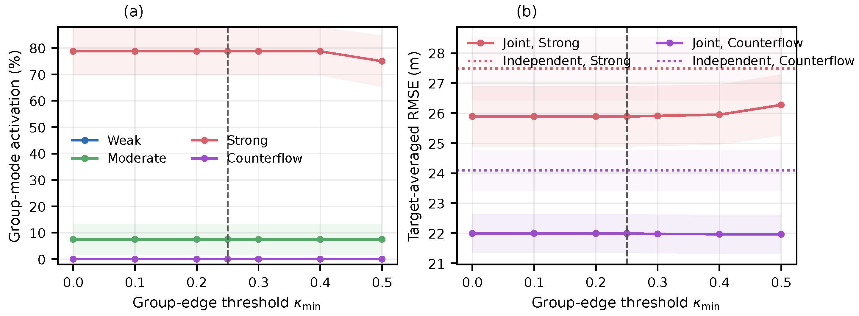
The threshold κ min [ 0 , 1 ] in Equation (25) sparsifies the global group-evidence edge-discovery path by setting subthreshold group scores to zero. Separately validated pair-relation hypotheses remain subject to distinct history-fit and held-out reliability criteria. Consequently, κ min is not a universal switch over every relation path.
The coupling weights determine the pair interaction factors inserted into the active graph and the corresponding MAP information contributions. Each forecast-origin computation first solves the target-local history graph without active pair factors. The history-only fit then determines the coupling scores and pair references used to assemble the final joint MAP problem. The preliminary fit uses no future measurement and is not reported as an independent estimator. Within a single MAP solve, K i c is fixed at the current forecast origin and is recomputed only before the next forecast-origin solve. The active pair set is E i c = { ( j , l ) : 1 j < l N B , κ j l , i > 0 } . No separately tuned coupling summary is fed back into the estimator.
The pair interaction factor is weighted by K i c . Define the relative-position and behavior differences by Δ ρ j l , k = ρ k B j ρ k B l and Δ m j l , k b = m j , k b m l , k b . References for both differences are obtained from the history-only fit at the current forecast origin and held fixed during the inner solve:
Δ ρ ¯ j l , k h = ρ ^ j , k h ρ ^ l , k h , Δ m ¯ j l , k b , h = m ^ j , k b , h m ^ l , k b , h .
where superscript h denotes a history-window estimate based on the finite graph at the current forecast origin before the pair reference is fixed. Both references are known during the current MAP solve, without employing any measurement later than t i or implying that a posterior from forecast origin i 1 is carried into forecast origin i. Stacking the position and behavior blocks yields the following:
r k , j l pair = κ j l , i Δ ρ j l , k Δ ρ ¯ j l , k h Δ m j l , k b Δ m ¯ j l , k b , h , Q pair = blkdiag σ pair , ρ 2 I 3 , σ pair , m 2 I n η .
Substituting the pairwise residual r k , j l pair from Equation (27) and the information matrix Q pair 1 into the generic Gaussian factor form in Equation (11) yields the pair factor ϕ k , j , l pair . The history-derived pair references and block covariance are kept identical in the Independent/Joint comparison. If  κ j l , i = 0 , Equation (27) vanishes and the corresponding pair factor contributes no information. The square-root weight in Equation (27) scales the information contribution linearly with the coupling score because κ r Q 1 2 = κ r T Q 1 r . Thresholding suppresses pair information when the history does not support a cross-target relation.
At each forecast origin, κ j l , i is recomputed from measurements no later than t i using Equations (23)–(25) and fixed during the solve. Thus, future truth is excluded from the coupling update.

2.2.6. Dynamics-Consistent Future Transition Factor

After solving the history-window posterior, each target is propagated through the augmented dynamics in Equation (7). Set y ˇ i B j = y i B j , e ˇ j , i i = clip [ 0 , 1 ] ( e ^ j , i ) , and  e ˇ j , k + 1 i = κ e e ˇ j , k i when no future measurement evidence is available. For k = i , , i + L p 1 , the normalized Markov transition factor under the independent-innovation baseline defines the complete conditional kernel:
ϕ k , j pred : = N y ˇ k + 1 B j ; A k η , j y ˇ k B j , Q k , j y ( e ˇ j , k i ) , p Y ˇ i + 1 : i + L p Θ i a , Z 0 : i = j = 1 N B k = i i + L p 1 ϕ k , j pred .
where Y ˇ i + 1 : i + L p = { y ˇ i + 1 : i + L p B j } j = 1 N B .
Equation (28) is conditional on the current active variables. Integrating the conditional kernel against the solved historical posterior gives the marginal future distribution:
p ( Y ˇ i + 1 : i + L p Z 0 : i ) = p ( Y ˇ i + 1 : i + L p Θ i a , Z 0 : i ) p ( Θ i a Z 0 : i ) d Θ i a .
The product kernel does not imply marginal independence. Equation (29) propagates historical dependence through the joint posterior into future means and covariance blocks. Marginal ellipsoids use diagonal blocks, whereas relative-position uncertainty also uses cross-target blocks. Consistent with the transition-only formulation, no target-pair reference factor is imposed after t i .

2.2.7. Factorization

Let Z 0 : i = { z k , j : 0 k i , 1 j N B } denote the measurement history. With the previously defined k 0 = i L h , we define the following:
K i 0 = { k 0 , , i } , K i = { k 0 , , i 1 } , K i + = { k 0 + 1 , , i } ,
The superscripts −, 0, and + label transition-departure, complete-window, and transition-arrival epoch sets, respectively; the superscripts do not denote prior and posterior updates. Here, K i b = { k K i 0 : k L b k 0 } . Let Θ i , k 0 entry collect the blocks of Θ i a at the first active epoch, and let Θ ¯ i , k 0 entry and P i , k 0 entry 0 denote the configured entry mean and covariance. The proper Gaussian entry potential is
Ψ i entry Θ i , k 0 entry exp 1 2 Θ i , k 0 entry Θ ¯ i , k 0 entry ( P i , k 0 entry ) 1 2 .
The entry potential makes explicit the boundary information already represented by F i entry and does not introduce an additional factor. The preceding coupling-weight subsection defines the active pair set E i c . The entry potential and active pair set yield the historical/current posterior factorization:
p ( Θ i a Z 0 : i ) Ψ i entry k K i ϕ k A , d j = 1 N B k K i ϕ k , j B , d j = 1 N B k K i 0 ϕ k , j z j = 1 N B k K i ϕ k , j η · j = 1 N B k K i + ϕ k , j b , d j = 1 N B k K i b ϕ k , j b , η j = 1 N B k K i + ϕ k , j e · ( j , l ) E i c k K i 0 ϕ k , j , l pair .
Let F i denote the set of all factor instances appearing in Equation (31). Composing Equation (31) with the transition kernel in Equation (28) yields the future predictive distribution without a second history-fitted motion model.
Two models are defined: Independent SOIR and Joint SOIR. Independent SOIR retains all target-local factors and the same dynamics-based prediction kernel, but it solves one chaser–target chain per object and sets the cross-target pair paths to zero. Joint SOIR retains one shared chaser chain and the active pair factors in the same posterior.
The resulting hierarchy separates the optimized graph states, history-updated coupling quantities, calibrated inputs, and propagated future moments.
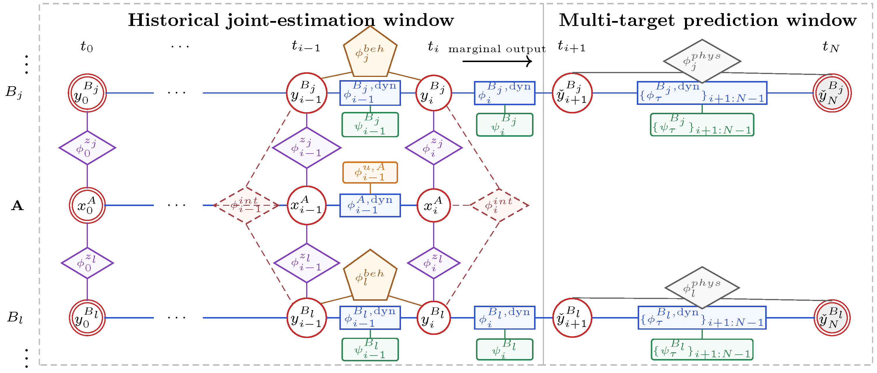
For the transition-only interface, Figure 1 provides a compact counterpart of Equation (31). Blue modules represent { ϕ A , d , ϕ B , d } , purple modules represent ϕ z , each brown ϕ beh aggregates { ϕ η , ϕ b , d , ϕ b , η , ϕ e } , and red dashed ϕ int modules represent active ϕ pair paths. The entry potential is implicit at the left boundary, while ϕ u , A marks a known conditioned input. Future blue chains and the gray/green support nodes denote the prediction and reachable-set interfaces rather than additional posterior likelihoods. All factor families of this historical-window construction are displayed explicitly or through the stated aggregates.

2.2.8. Local Markov Blanket and Conditional Independence

For a variable block ϑ , only factors whose scopes contain ϑ contribute to the conditional density. The graph Markov blanket of ϑ is therefore the union of the remaining variables in the incident factor scopes. For a current target state, the Markov blanket contains the adjacent dynamics, current measurement, maneuver, behavior, event, and active pair variables. Future states are conditional outputs of the historical-window MAP problem and are generated by the target-local transition kernel in Equation (28). Shared-state and pair information enter prediction through the solved target means, marginal covariances, and cross-covariance blocks, rather than through future truth or unavailable measurements.

2.3. Joint Posterior and Time-Indexed Reachable Sets

2.3.1. Historical-Window MAP Estimation

At one outer relinearization, the restricted event values, event-evidence energies, and event-dependent factor information matrices are fixed before the inner solve. The coupling scores and pair references are computed once at the current forecast origin and remain fixed throughout the nonlinear MAP solve. Conditional on the fixed quantities, taking the negative logarithm of Equation (31) and substituting the residual energies defined above yields the explicit MAP subproblem. Normalization terms that are constant with respect to the active variables do not affect the optimizer, giving
Θ i = arg max Θ i a p ( Θ i a Z 0 : i ) = arg min Θ i a J i ( Θ i a ) , J i = 1 2 { Θ i , k 0 entry Θ ¯ i , k 0 entry ( P i , k 0 entry ) 1 2 + k K i r k A , d ( Q k A , d ) 1 2 + j = 1 N B k K i r k , j B , d ( Q k , j B , d ) 1 2 + j = 1 N B k K i 0 r k , j z ( R k , j e ) 1 2 + j = 1 N B k K i r k , j η GM [ Q k , j η ( e ˜ j , k ) ] 1 2 + r k , j η E Q η E 1 2 + r k , j η Q η 1 2 + j = 1 N B k K i + r k , j b , d Q m 1 2 + j = 1 N B k K i b r k , j b , η Q b 1 2 + j = 1 N B k K i + r k , j e , d r k , j e , z r k , j e , l i m Q e 1 2 + ( j , l ) E i c k K i 0 r k , j l pair Q pair 1 2 } .
Equation (32a) contains only the factors defined above and therefore introduces no additional cost term. For a fixed outer configuration, Equation (32a) is a conditional MAP problem. The reported estimate is conditioned on the final accepted configuration and does not jointly optimize the history-derived scores and covariance arguments.
At forecast origin i, r indexes the outer configuration refresh and s it indexes the inner nonlinear iteration. History-derived pair quantities, entry priors, measurement covariances, and calibration constants remain fixed. Let col ( · ) denote vertical concatenation in lexicographic ( j , k ) order. The interval-clipping and event-evidence functions defined above give
c i ( r ) : = col { e ˜ j , k ( r ) , e ¯ j , k ( r ) } 1 j N B , k K i 0 [ 0 , 1 ] 2 N B | K i 0 | , G i ( Θ i a ) : = col { clip [ 0 , 1 ] ( e j , k ) , e ¯ j , k ( Θ i a ) } 1 j N B , k K i 0 .
The energies in Equation (20) are intermediate evaluations within G i and are not additional configuration coordinates. All entries of Θ i a , including e j , k and the maneuver states, remain optimization variables. During one inner solve, only e ˜ j , k and e ¯ j , k are held fixed as covariance arguments and evidence targets.
Let J i denote the objective in Equation (32a). The ideal conditional solution map and the associated outer map are
S i ( c ) = argmin Θ i a J i ( Θ i a ; c ) , T i , ω ( c ) = ( 1 ω ) c + ω G i S i ( c ) , 0 < ω 1 , c i ( r + 1 ) = T i , ω ( c i ( r ) ) .
For each fixed c i ( r ) , the inner Gauss–Newton/Levenberg–Marquardt iterations compute an accepted finite-iteration approximation to S i ( c i ( r ) ) by minimizing the conditional objective J i ( Θ i a ; c i ( r ) ) . Equation (61) specifies the inner stopping test, and  Section 2.3.5 specifies the damping, acceptance, and failure-handling rules. Only an accepted inner solution is supplied to G i . The subsequent evaluation of G i is a deterministic configuration-consistency refresh rather than a second optimization step. The raw refresh is under-relaxed when 0 < ω < 1 , whereas ω = 1 applies it directly. Thus, SolveMap nests conditional minimization within a fixed-point configuration update. Because the configuration refresh is not required to decrease a common objective across outer iterations, the complete procedure is not claimed to be a block-coordinate descent or majorization–minimization algorithm.
On a fixed soft-limit branch, suppose that the conditional objective has a positive-definite Hessian with strong-convexity modulus m i > 0 , as characterized by the positive-definiteness argument below. The corresponding ideal map S i is then single-valued. Suppose further that S i is Lipschitz on the compact hypercube in Equation (32b) with constant L S , i , and that G i is Lipschitz on the corresponding bounded solution image with constant L G , i . If
L T , i , ω : = 1 ω + ω L G , i L S , i < 1 , c i ( r ) c i 2 L T , i , ω r c i ( 0 ) c i 2 , c ˜ i ( r + 1 ) c i 2 L T , i , ω c ˜ i ( r ) c i 2 + δ r ,
Here, c ˜ i ( r ) denotes the sequence generated by the finite inner solves, and  δ r bounds the corresponding error in the configuration refresh. Under the stated local assumptions and L T , i , ω < 1 , the contraction principle guarantees a unique local fixed point for the ideal outer map. If  δ r 0 , the  inexact iteration converges to the same fixed point. If only δ r δ ¯ is available, then
lim sup r c ˜ i ( r ) c i 2 δ ¯ 1 L T , i , ω .
The strict contraction inequality is an additional sufficient condition; bounded covariances, under-relaxation, and a small observed update do not by themselves establish it. This condition is analytical rather than an operational stopping test. The implementation does not estimate L S , i , L G , i , or  L T , i , ω . Instead, the inner solve is terminated according to Equation (61), and the outer configuration is accepted when the observable consistency residual satisfies r out , i ( r ) ε out , as specified in Section 2.3.5. The convergence result therefore characterizes the ideal outer map under the stated contraction assumption; however, without numerical bounds on L T , i , ω and δ ¯ , the  quantity δ ¯ / ( 1 L T , i , ω ) is not used as a computed a posteriori error radius.
For the transition-only historical-window objective in Equation (32a), future states are conditional outputs rather than additional observations or history-window optimization variables. Therefore, prediction factors are excluded from the MAP objective.
After linearization, we have the following:
δ Θ i = arg min δ Θ i W i 1 / 2 ( J i δ Θ i + r ^ i ) 2 2 ,
Here, r ^ i denotes the stacked residual evaluated at the current linearization point, J i is the corresponding stacked Jacobian, and  W i represents the block-diagonal matrix containing the associated factor information matrices. In terms of the target dynamics, we obtain the following:
r k , j B , d r ^ k , j B , d + δ x k + 1 B j F k B j δ x k B j G k B j δ η k B j .
Λ i = ζ F i J ζ T Ω ζ J ζ , ξ i = ζ F i J ζ T Ω ζ r ^ ζ , Λ i δ Θ i = ξ i .    
The covariance used below is the local Laplace–Gauss–Newton approximation evaluated at the converged mode.
For the relative-position interface in Equation (9), fixing the outer configuration makes the stated measurement, transition, behavior, and pair residuals affine. The soft-limit residuals are also affine within each smooth branch. Consequently,
Θ 2 J i = ζ J ζ T Ω ζ J ζ = Λ i .
Within a fixed active branch, the residual Jacobians are constant, so Λ i is the exact Hessian of the conditional quadratic objective and introduces no additional linearization-curvature error on that branch. This conclusion is local: initialization and branch switching can affect the accepted solution, while upstream reconstruction error and dynamics mismatch remain outside the guarantee. The Hessian identity therefore does not imply a globally Gaussian posterior, and moment-preserving propagation does not by itself guarantee empirical coverage.

2.3.2. Posterior Prediction

Let y ^ i B j and P j l , i B be the current target means and covariance blocks extracted from the solved joint posterior. Specifically, the Boolean selectors defined later in Equation (62) give y ^ i B j : = μ i B j = S j y Θ ^ i , e ^ j , i = S j e Θ ^ i , and  P j l , i B = S j y P Θ , i ( S l y ) T . The diagonal blocks initialize target-wise propagation, whereas the off-diagonal blocks retain the cross-target dependence induced by the shared chaser and active historical pair paths.
The augmented transition product is defined by
Φ j , b : a B = A b 1 η , j A b 2 η , j A a η , j , b > a , I 6 + n η , b = a .
At forecast origin i, future observations are unavailable and future process innovations have not yet been realized. This lack of information does not imply physical independence. Rather, without an additional predictive model, the available history alone does not uniquely determine the future cross-innovation covariance kernel. The independent-innovation baseline therefore assumes that the future process innovations { υ k , j y } are zero mean and conditionally independent across future epochs and targets given Z 0 : i . The stacked future innovation sequence is also assumed to be conditionally independent of the forecast-origin joint state given Z 0 : i . History-supported posterior dependence is nevertheless retained in the initial cross-covariance blocks P j l , i B and subsequently propagated by the state-transition model. In addition, the conditional mean of the equivalent maneuver retains the Gauss–Markov memory specified by κ η in Equation (6). Under these assumptions, the baseline recursion is initialized by ( μ i i B j , P i i B j ) = ( y ^ i B j , P j j , i B ) , and the moments propagate as follows:
μ k + 1 i B j = A k η , j μ k i B j , P k + 1 i B j = A k η , j P k i B j ( A k η , j ) T + Q k , j y ( e ˇ j , k i ) , k = i , , i + L p 1 .
Let Π j , τ ρ denote τ applications of Equation (37), followed by the position marginal in Equation (39). The propagation operator satisfies
( μ ρ , i + τ B j , P ρ , i + τ B j ) = Π j , τ ρ ( y ^ i B j , P j j , i B , e ^ j , i ) .
The propagation operator introduces neither an additional motion model nor covariance inflation beyond the stated recursion. For  j l , independent future process innovations yield
P j l , i + τ i B , 0 = Φ j , i + τ : i B P j l , i B ( Φ l , i + τ : i B ) T .
Under the independent-innovation baseline, future target dependence is inherited from the current joint posterior rather than introduced through a fitted future reference.
To expose the terms omitted by the independent-innovation baseline, consider zero-mean future disturbances with finite second moments and conditional covariance blocks
Q j l υ ( s , u ) : = Cov υ s , j y , υ u , l y Z 0 : i , s , u = i , , i + L p 1 .
Require Q j l υ ( s , u ) = [ Q l j υ ( u , s ) ] T , Q j j υ ( s , s ) = Q s , j y ( e ˇ j , s i ) , and a positive-semidefinite stacked covariance. With the forecast-origin joint state conditionally independent of the entire future sequence, for all j , l ,
P j l , i + τ i B , Q = Φ j , i + τ : i B P j l , i B ( Φ l , i + τ : i B ) T + s = i i + τ 1 u = i i + τ 1 Φ j , i + τ : s + 1 B Q j l υ ( s , u ) ( Φ l , i + τ : u + 1 B ) T .
The superscripts 0 and Q denote, respectively, the independent-innovation baseline and propagation with the specified covariance kernel Q j l υ ( s , u ) ; they are not labels for the Independent and Joint SOIR estimators. Retaining the prescribed diagonal blocks and setting Q j l υ ( s , u ) = 0 for ( j , s ) ( l , u ) reduces the generalized recursion to Equations (37) and (38). Blocks with s u represent temporal correlation and are required because a propagated state accumulates innovations from earlier epochs. Conditional dependence between the forecast-origin state and future innovations would introduce additional state–innovation cross terms.
Joint Gaussianity of the forecast-origin state and the stacked future innovation sequence, rather than Gaussian marginal laws alone, is sufficient for the Gaussian predicted-position law. When the diagonal innovation blocks are retained, cross-target innovation blocks leave the target-wise marginal moments unchanged but modify the relative-position covariance in Equation (60). The remaining position projection and CDIC construction are unchanged. This correlated-innovation model is an analytical extension; Algorithm 1 retains the independent-innovation recursion.
Algorithm 1 Finite-history joint posterior and dynamics-based reachable envelope construction
Require: 
Boundary t i , measurements Z 0 : i , entry priors, prediction length L p , confidence level α
Ensure: 
Target envelopes and propagated target covariance blocks
  1:
Obtain the target-local history fit from Z 0 : i
  2:
Update K i c , pair references, and  E i c from that fit
  3:
Assemble F i by Equation (31)
  4:
( Θ ^ i , Λ i , ξ i , status i )  SolveMap  ( F i , Θ i a )
  5:
if  status i converged  then
  6:
      return no envelope and a non-convergence flag
  7:
end if
  8:
Extract { y ^ i B j , e ^ j , i , P j l , i B } by Equation (62)
  9:
for  j = 1 to N B  do
10:
      for  τ = 1 to L p  do
11:
           Propagate ( μ ρ , i + τ B j , P ρ , i + τ B j ) Π j , τ ρ ( y ^ i B j , P j j , i B , e ^ j , i )
12:
        Construct E j , i + τ CDIC ( α ) and, when calibrated, the optional set-valued completion
13:
      end for
14:
end for
15:
Propagate cross-covariances by Equation (38)
Applying S ρ y to the first mean update in Equation (37) directly produces the first predicted position displacement without an additional direction or fitted future reference. Under the stated joint Gaussian conditions, projecting the propagated augmented state yields the position marginal
ρ i + τ B j N ( μ ρ , i + τ B j , P ρ , i + τ B j ) ,
where
μ ρ , i + τ B j = S ρ y μ i + τ i B j , P ρ , i + τ B j = S ρ y P i + τ i B j ( S ρ y ) T .

2.3.3. Corrected-Dynamics Inferred-Control Reachable Envelope

Let α ( 0 , 1 ) denote probability content under the local Gaussian law q j , τ , with P ρ , i + τ B j 0 , and let χ d 2 ( α ) be the corresponding chi-square quantile. We have
E j , i + τ CDIC ( α ) = ρ : ( ρ μ ρ , i + τ B j ) T ( P ρ , i + τ B j ) 1 ( ρ μ ρ , i + τ B j ) χ 3 2 ( α ) .
The posterior ellipsoid supplies the center and covariance component of the time-indexed region.
To allocate maneuver uncertainty without counting the same component twice, define the maneuver selector S η y = [ 0 n η × 6 I n η ] . The propagated maneuver moments are μ η , j , s i = S η y μ s i B j and P η , j , s i = S η y P s i B j ( S η y ) T . The corresponding covariance allowance and residual physical budget are
ς η , j , s p ( α η ) = χ n η 2 ( α η ) diag ( P η , j , s i ) , b η , j , s = η ¯ j | μ η , j , s i | ς η , j , s p ( α η ) + , Δ U η , j , s = δ η : | δ η | b η , j , s .
The allocation level α η determines b η , j , s and therefore, through Equation (42), the geometry of C j , i i + τ η . The set suppresses the dependence on α η for readability. The allocation level α η is neither equal to β η nor an additional probability multiplier. All operations in Equation (41) are componentwise, with ( a ) + : = max { a , 0 } .
The residual support maps into position space as follows:
C j , i i + τ η = s = i i + τ 1 S ρ y Φ j , i + τ : s + 1 B G s B j 0 n η × n η Δ U η , j , s .
Let r geom , j be the target’s geometric radius and r safe , j an additional operational margin. With r dil , j = r geom , j + r safe , j and B ( r ) : = { d R 3 : d 2 r } , the target-wise occupied region is
R j , i + τ CDIC ( α ) = E j , i + τ CDIC ( α ) C j , i i + τ η B ( r dil , j ) .
Appendix A derives a conservative ellipsoidal outer approximation for downstream set computations.
Let ρ i + τ B j , ctr be the true target-center position. An occupied point is represented by
ρ i + τ B j , occ = ρ i + τ B j , ctr + e dil , ρ i + τ B j , ctr μ ρ , i + τ B j = e G + e η .
Here, e G is the modeled posterior position error, e η is the displacement induced by unresolved residual maneuvers, and e dil is a physical offset.
Assumption 1
(Posterior and residual-support events). Conditional on Z 0 : i , the occupied-point error admits the decomposition in Equation (44) under the joint predictive measure P q , η . Define the component events
A G : = e G E j , i + τ CDIC ( α ) { μ ρ , i + τ B j } , A η : = e η C j , i i + τ η .
Under P q , η , the marginal law of e G is the centered local Gaussian law induced by q j , τ . For some β η [ 0 , 1 ] , assume that
P q , η ( A G Z 0 : i ) = α , P q , η ( A η Z 0 : i ) β η .
The allocation level α η determines the geometry of A η through the construction of b η , j , s and C j , i i + τ η , whereas β η is a separate lower bound on the conditional residual-support probability. Consequently, β η cannot be inferred from α η alone. Finally, the deterministic dilation error satisfies e dil B ( r dil , j ) .
The probability statement follows from the Fréchet–Hoeffding inequality and does not require conditional independence [31].
Proposition 1
(Target-wise CDIC containment). Under Assumption 1, every realization in A G A η produces an occupied point in the CDIC region of Equation (43). Moreover,
P q , η ρ i + τ B j , occ R j , i + τ CDIC ( α ) Z 0 : i max ( 0 , α + β η 1 ) .
Proof. 
For every outcome in A G A η , Equation (44) and the deterministic geometric bound give
ρ i + τ B j , occ = μ ρ , i + τ B j + e G + e η + e dil E j , i + τ CDIC ( α ) C j , i i + τ η B ( r dil , j ) = R j , i + τ CDIC ( α ) .
Taking conditional probabilities, using P q , η ( A G A η Z 0 : i ) 1 , and applying nonnegativity gives
P q , η ( ρ i + τ B j , occ R j , i + τ CDIC ( α ) Z 0 : i ) P q , η ( A G A η Z 0 : i ) = P q , η ( A G Z 0 : i ) + P q , η ( A η Z 0 : i ) P q , η ( A G A η Z 0 : i ) max ( 0 , α + β η 1 ) ,
The final inequality establishes Equation (47). □
Remark 1
(Dependence-free interpretation). With only the two marginal event probabilities, [ α + β η 1 ] + is sharp for A G A η , but not necessarily for the larger complete-CDIC event; no independence is required. Setting β η = 1 requires almost-sure residual containment, after which the lower bound is α.
Proposition 1 is a conditional predictive-model statement. The proposition does not equate the nominal level with frequentist truth coverage, which is assessed separately in Section 3.
Under the local Laplace approximation for extracting the posterior moments, we obtain the following:
q j , τ ( ρ Z 0 : i ) = N ( μ ρ , i + τ B j , P ρ , i + τ B j ) , E j , i + τ CDIC ( α ) q j , τ ( ρ Z 0 : i ) d ρ = α .
Finally, the target and scenario tubes retain both the object and time indices:
R j , i CDIC ( α ) = τ = 1 L p R j , i + τ CDIC ( α ) × { t i + τ } , O i S ( α ) = τ = 1 L p j = 1 N B R j , i + τ CDIC ( α ) × { t i + τ } .
The physical space–time union is not a joint confidence region. At one prediction time, simultaneous multi-target containment is the event intersection
j = 1 N B ρ i + τ B j , occ R j , i + τ CDIC ( α ) .
The conditional probability of this intersection is not determined by α . Extending the intersection over prediction times gives target–time simultaneous coverage, whose probability also differs from the per-target all-query frequency in Section 3.

2.3.4. Joint Posterior Marginalization and Reachability Mapping

For the independent-innovation baseline, cross-target dependence is inherited from the solved MAP system rather than introduced by a post-processing scale. Let Θ B collect all target-specific state, maneuver, behavior, and event variables, and let Θ sh collect the shared chaser chain. Boolean selectors S B and S sh extract the two aggregate blocks from the active ordering. Define Λ U V = S U Λ i S V T and ξ U = S U ξ i for U , V { B , sh } .
Assumption 2
(Anchored local information structure). At the accepted fixed outer configuration, every active coordinate belongs to a complete transition chain with a proper positive-definite entry prior and positive-definite transition covariances. All remaining Gauss–Newton factor contributions are positive semidefinite.
To establish positive definiteness, let L i denote the stacked entry and transition residual Jacobians from Assumption 2. If L i v = 0 , the entry rows force the first perturbation of every active chain to zero, and the transition rows recursively force all subsequent perturbations to zero. Hence, L i has full column rank. Let w i > 0 be a common lower bound on the minimum eigenvalues of the entry and transition information matrices. Since all remaining factor contributions are positive semidefinite,
v T Λ i v w i L i v 2 2 m i v 2 2 > 0 , v 0 , m i : = w i σ min ( L i ) 2 > 0 .
Therefore, Λ i 0 on the selected active coordinates. This is a structural exact-arithmetic result; numerical conditioning and covariance admissibility are checked separately in Section 2.3.5.
Partitioning the positive-definite active information system according to the target-specific and shared-state coordinates gives
Λ B B Λ B sh Λ sh B Λ sh sh δ Θ B δ Θ sh = ξ B ξ sh .
The block Λ B B contains the target-local factors and all active direct pair factors, whereas the off-diagonal blocks represent the connections between the target variables and the common uncertain chaser states. Since Λ i 0 , its shared principal block satisfies Λ sh sh 0 and is therefore invertible. The associated target Schur complement is consequently well defined and positive definite [32]. Proposition 2 gives the resulting reduced target system and identifies the dependence induced by eliminating the shared variables.
Proposition 2
(Shared-variable reduced information). Under Assumption 2, eliminating the shared block produces the reduced target system
Λ B m δ Θ B = ξ B m , P B m = ( Λ B m ) 1 ,
where
Λ B m = Λ B B Λ B sh Λ sh sh 1 Λ sh B , ξ B m = ξ B Λ B sh Λ sh sh 1 ξ sh .
For j l , the off-diagonal target block of Λ B m is
[ Λ B m ] j l = [ Λ B B ] j l Λ B j sh Λ sh sh 1 Λ sh B l .
Thus direct pair factors and uncertain shared variables are two distinct sources of target dependence in the reduced information matrix.
Proof. 
The positive-definite system in Equation (52) has the following block rows:
Λ B B δ Θ B + Λ B sh δ Θ sh = ξ B , Λ sh B δ Θ B + Λ sh sh δ Θ sh = ξ sh .
The positive definiteness of Λ sh sh permits the solution of the second row as follows:
δ Θ sh = Λ sh sh 1 ξ sh Λ sh B δ Θ B .
Substituting Equation (57) into the first row of Equation (56) yields
Λ B B Λ B sh Λ sh sh 1 Λ sh B δ Θ B = ξ B Λ B sh Λ sh sh 1 ξ sh ,
The substitution identifies Λ B m and ξ B m in Equation (54). Inverting the reduced precision yields the exact target marginal covariance P B m of the stated local Gaussian model. Selecting the ( j , l ) target block of Equation (54) yields Equation (55). □
Corollary 1
(Vanishing-coupling limit). For every j l , suppose that
[ Λ B B ] j l = 0 , Λ B j sh Λ sh sh 1 Λ sh B l = 0 .
Then the reduced Joint information matrix Λ B m and the corresponding covariance P B m are block diagonal across targets. In common increment coordinates about the same linearization anchor, the factorized limit coincides target by target with separately constructed target-wise posteriors if and only if
[ Λ B m ] j j = Λ B j Ind , [ ξ B m ] j = ξ B j Ind for all j .
Proof. 
Equation (55) and the stated conditions lead to [ Λ B m ] j l = 0 for j l . Positive definiteness then implies P B m = blkdiag j ( [ Λ B m ] j j 1 ) . In common increment coordinates, a Gaussian posterior is uniquely specified by the posterior information matrix and information vector. Hence, target-wise equality is equivalent to Equation (59). □
The off-diagonal conditions hold, for example, when direct pair factors are absent and the shared block can be permuted into mutually disjoint target-specific blocks, with target B j connected only to the corresponding block. Exact agreement with a separately solved A- B j chain additionally requires the same factors, priors, linearization anchor, and Gaussian weights. Consequently, block decoupling is weaker than target-wise equality with a separately solved model.
Remark 2
(Undamped covariance interpretation). At the final accepted configuration and active branch, Proposition 2 gives the exact target marginal covariance of the local Gaussian approximation. The reported covariance is formed from the final undamped, unregularized information matrix. The diagonal equilibration in Equation (62) is an invertible congruence scaling of that matrix; it is not statistical regularization and alters neither the MAP mode nor the covariance after transformation back to the original coordinates. LM damping is likewise excluded from the reported posterior information matrix. If the undamped matrix or a required selected covariance fails the stated positive-definiteness checks, the corresponding query is rejected rather than replaced by a regularized Gaussian approximation.
For fixed i and k i , write P j l ρ : = S ρ y P j l , k i B ( S ρ y ) T , with P j l , i i B = P j l , i B . Suppressing the time indices and conditioning on Z 0 : i , the relative-position covariance is
Cov ( ρ B j ρ B l ) = P j j ρ + P l l ρ P j l ρ P l j ρ .
Independent estimation replaces the single shared chaser chain with one target-local chaser copy per A- B j solve and removes direct pair paths; the Independent information system therefore contains no cross-target blocks. Joint estimation retains the common chaser chain and active pair paths in the same MAP solve. The extracted Joint blocks initialize Equations (37) and (38).

2.3.5. Numerical MAP Solution and Reachable-Envelope Construction

At each forecast origin, SolveMap processes the historical/current factor graph as a separate batch problem whose bounded internal procedure may contain several configuration refreshes. After a successful solve, the target marginals are propagated to the common endpoint. Earlier separator potentials and posteriors are not carried forward between forecast origins.
The active factors at origin i form F i in the MAP objective. The prediction kernel is applied only after the active factor set is solved and is not another measurement or pseudo-measurement.
At each forecast origin, the active vector is initialized from the configured entry priors and measurement-conditioned history estimates. The outer configuration c i ( r ) , the refresh map G i , and the indices i, r, and s it are defined in Equations (32b) and (32c). The additional index LM denotes an LM damping trial within inner iteration s it . Evaluating G i at the initialized active vector gives c i ( 0 ) . Pair coefficients and references are computed once from the target-local history fit and remain fixed throughout both the inner solve and the subsequent configuration refreshes. The following numerical procedure specifies the finite-iteration realization of S i used by SolveMap. It does not redefine the outer map T i , ω .
For fixed c i ( r ) , all non-hinge residuals in Equation (32a) are affine in the active variables, and each hinge residual is affine once its activation state and, for an active component, its sign are fixed. The conditional objective is therefore piecewise quadratic. At inner iterate Θ i ( s it ) , let f i ( s it ) denote the stacked whitened residual and J i ( s it ) its Jacobian, and define
H i ( s it ) = ( J i ( s it ) ) T J i ( s it ) , g i ( s it ) = ( J i ( s it ) ) T f i ( s it ) .
The inner solver first evaluates the Gauss–Newton step
H i ( s it ) δ Θ i ( s it ) = g i ( s it ) .
If the Gauss–Newton candidate fails a finite-value, objective-acceptance, or scaled normal-equation residual check, the Levenberg–Marquardt recovery is initialized from the same fixed-configuration starting point and computes
H i ( s it ) + λ s it , LM I δ Θ i ( s it , LM ) = g i ( s it ) , λ s it , LM > 0 .
The corresponding gain ratio is
ρ s it , LM = J i ( Θ i ( s it ) ; c i ( r ) ) J i ( Θ i ( s it ) + δ Θ i ( s it , LM ) ; c i ( r ) ) ( g i ( s it ) ) T δ Θ i ( s it , LM ) 1 2 ( δ Θ i ( s it , LM ) ) T H i ( s it ) δ Θ i ( s it , LM ) .
It compares the actual objective reduction with that predicted by the local quadratic model. A trial is accepted only if both reductions are finite and strictly positive and ρ s it , LM ρ min . For β λ > 1 , acceptance sets the initial damping for the next inner iteration to max ( λ s it , LM / β λ , λ lo ) . Rejection increases the damping for the current inner iteration to min ( β λ λ s it , LM , λ hi ) , after which the trial step is recomputed. The corresponding numerical values and iteration caps are reported with the simulation settings in Section 3.1.
Let ε Θ > 0 and ε J > 0 denote the step and relative-objective tolerances, and let N it denote the applicable nonlinear-iteration cap. Inner iteration s it stops when
δ Θ i ( s it ) ε Θ or | J i ( s it ) J i ( s it 1 ) | max ( 1 , J i ( s it 1 ) ) ε J .
If neither condition holds by N it , the solve is classified as non-convergent. The returned branch is accepted only when all returned quantities are finite, the accepted candidate satisfies the declared objective criterion, and the scaled normal-equation residual is below ε NE . Write the final affine branch as A i Θ i b i , with H i = A i T A i , h i = A i T b i , and D i n = diag ( [ H i ] q q 1 / 2 ) . The scaled residual is
r NE , i = D i n ( H i Θ ^ i h i ) 1 + D i n h i ε NE .
After an accepted inner solution, the interval-clipping and evidence formulas define the deterministic refresh map G i :
c i , raw ( r + 1 ) = G i ( Θ ^ i ( r ) ) , r out , i ( r ) = c i , raw ( r + 1 ) c i ( r ) , c i ( r + 1 ) = ( 1 ω ) c i ( r ) + ω c i , raw ( r + 1 ) , r out , i ( r ) > ε out .    
The current inner solution is accepted when r out , i ( r ) ε out . Otherwise, the under-relaxed update is used. The index r is a fixed-point consistency counter at one forecast origin and is not an additional history epoch. Exhausting an inner or outer budget, or failing an acceptance check, returns an unsuccessful status in Algorithm 1.
Let S j y and S j e select the current target and event blocks.
Covariance is extracted only after both convergence levels succeed. For the final fixed configuration and active branch, let Λ i = A i T A i be the undamped information matrix. Retaining the manuscript’s information-matrix interface, write Λ ¯ i = Λ i + ε cov D i , where D i 0 is the retained diagonal scaling matrix and ε cov 0 . The reported calculations use the unregularized case Λ ¯ i = Λ i ; Section 3 lists the corresponding numerical setting. A failed positive-definiteness check is not repaired by additive regularization. When the diagonal entries of Λ ¯ i are positive and finite, diagonal equilibration gives the same inverse in balanced coordinates:
D i n = diag ( [ Λ ¯ i ] q q 1 / 2 ) , B i = D i n Λ ¯ i D i n 0 , P Θ , i = D i n B i 1 D i n , μ i B j = S j y Θ ^ i , e ^ j , i = S j e Θ ^ i , P j l , i B = S j y P Θ , i ( S l y ) T .
The balanced matrix is factorized using a sparse L D L T decomposition with positive finite pivots, and only the covariance columns required by the selectors are solved and symmetrized. Diagonal equilibration is a reversible coordinate scaling, not posterior regularization. LM damping is excluded from Λ i ; in the reported calculations, no ridge, pseudoinverse, or eigenvalue floor is used. If the undamped factorization, a selected solve, or a propagated position block is nonfinite or non-positive definite, the query is rejected and no reachable region is generated.
Let L = L h + 1 be the number of active history/current epochs, and let d c be the maximum active pair degree. Since the active vector in Equation (12) contains one six-dimensional chaser state and, per target, one ( 6 + n η ) -dimensional augmented state, one n η -dimensional behavior state, and one scalar event state at each epoch, the scalar variable and residual dimensions satisfy the following:
n Θ , i = L 6 + N B ( 7 + 2 n η ) , n r , i = O L N B + L | E i c | = O L N B ( 1 + d c ) .
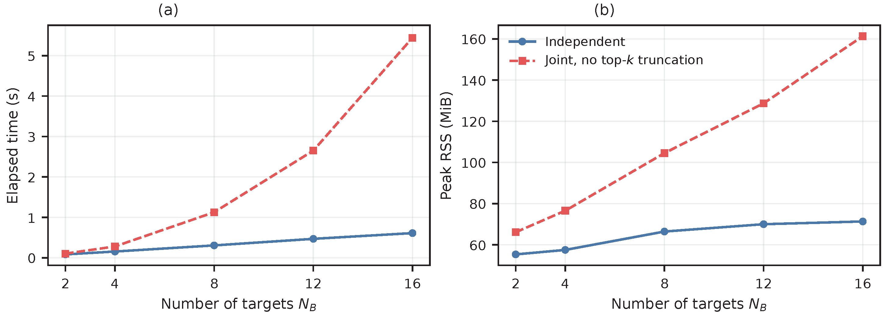
Sparse factorization imposes a cost O ( c | C c | 3 ) over elimination cliques C c , with the conservative dense upper bound of O ( n Θ , i 3 ) . Direct moment propagation imposes a cost O ( N B L p ) for a fixed state dimension. Propagating the complete target cross-covariance matrix imposes a cost O ( N B 2 L p ) because the shared chaser can induce nonzero blocks even between targets without a direct pair edge. If only a declared query set Q i of covariance blocks is required, the corresponding cost is O ( | Q i | L p ) . Here, | C c | denotes the number of scalar degrees of freedom in clique C c , not merely the number of variable nodes.

3. Results

This section evaluates probabilistic reachable-region prediction under different cross-target relation patterns. Independent SOIR is the reference estimator applied target-wise: it estimates each chaser–target chain separately and removes cross-target information paths. Joint SOIR retains the shared chaser state and history-supported pair relations in one posterior, allowing transfer of information supported by measurements across targets. The simulations assess target-matched coverage, prediction-center error, region compactness, and time-indexed 3D envelopes. Additional experiments examine insufficient, persistent, signed, and mismatched relation evidence, as well as different history–forecast allocations.
The archived CDIC experiments use an implementation that augments the transition-only forecast with soft relative-state constraints fitted from history whose weights decay over the prediction horizon. The prediction-node constraints use neither future observations nor future truth and are not part of Algorithm 1. Accordingly, the main Monte Carlo results characterize the implementation-specific extension, whereas the innovation-kernel check isolates the covariance-propagation law under the conditional model.

3.1. Simulation Design

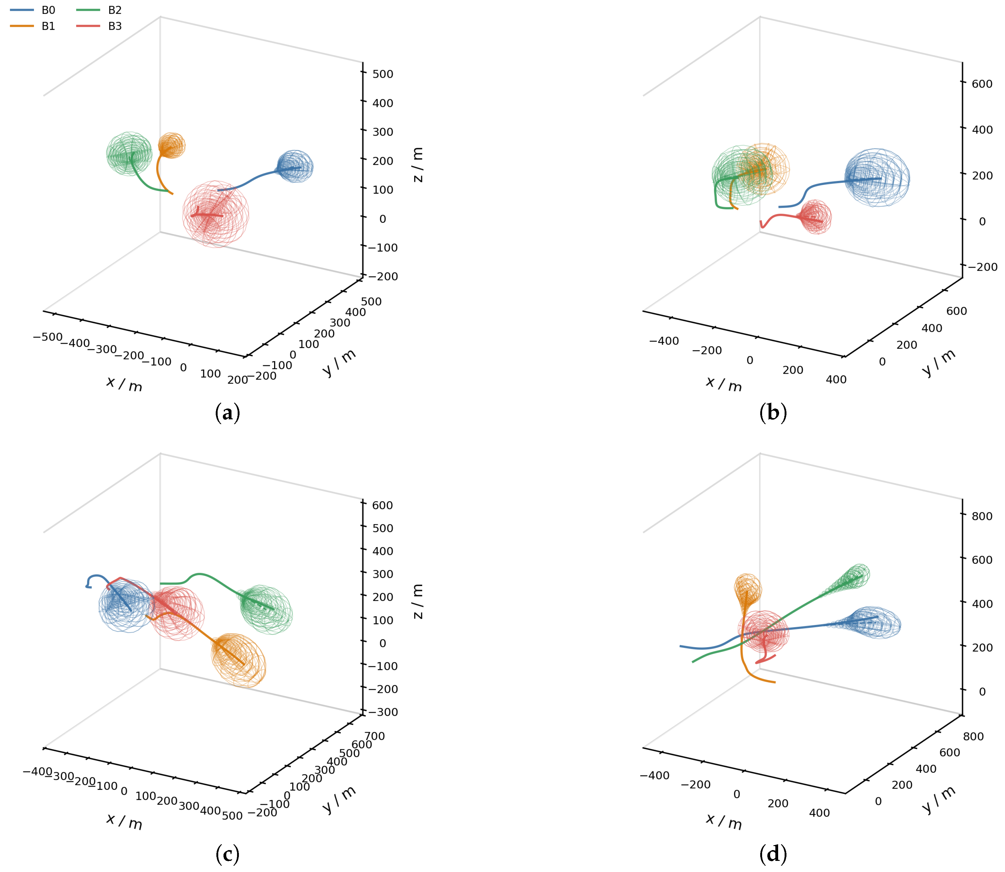
Four three-dimensional multi-target scenarios represent insufficient, partial, persistent, and signed historical relations: Weak, Moderate, Strong, and Counterflow. These mechanism-controlled cases isolate how the amount, persistence, and sign of historical relation evidence affect estimation and prediction; they are not treated as a random operational population. All methods receive identical target identities, time stamps, relative-position observations, validity masks, and seed-indexed truth realizations. Scenario labels, command coefficients, future truth, and coverage outcomes remain unavailable to the estimators.
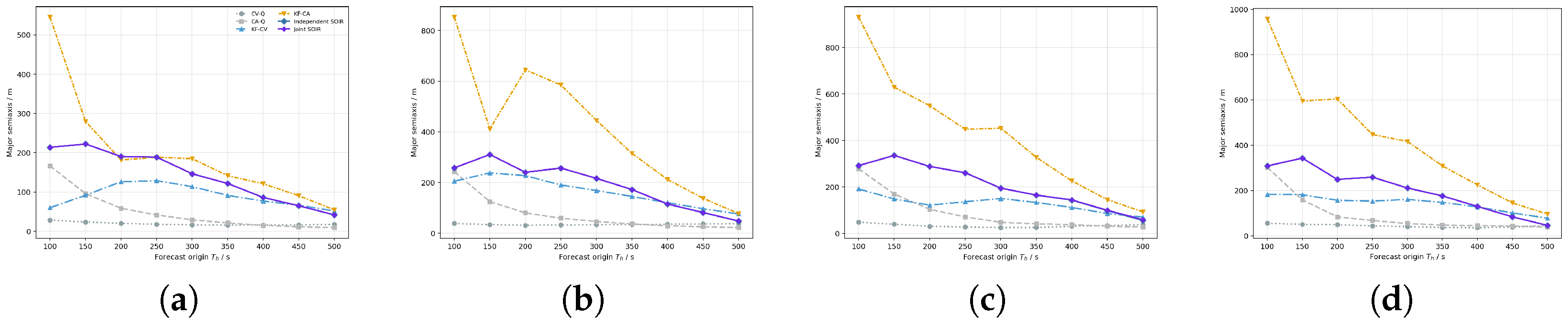
The experiments are organized to answer distinct questions. The primary Monte Carlo comparison evaluates accuracy, coverage, and region size under the four controlled relation regimes. Varying the forecast origin examines the combined effect of accumulated history and prediction duration. Parameter sweeps quantify the local sensitivity of relation activation, posterior uncertainty, and Joint-versus-Independent performance with respect to calibration values. An ensemble of continuously sampled configurations assesses whether the observed behavior extends beyond the four mechanism-controlled scenarios within the declared simulation domain. A target-count experiment examines accuracy retention and computational-resource growth as the number of non-cooperative targets increases. The implementation used Python 3.10.12 and C++17. It was evaluated on an Intel Core i7-7700HQ processor, with eight logical processors available at a fixed level of parallelism. End-to-end time and peak resident set size (RSS) quantify computational cost and memory demand.
Each controlled scenario contains N B = 4 non-cooperative targets and M = 160 independent Monte Carlo runs indexed by seed. Each simulation forms the sampling unit; its targets and query times are repeated measurements rather than additional independent samples. Identical stochastic inputs for each seed provide comparisons across methods and forecast origins. The 10,000 bootstrap repetitions resample the 160 realization-level units and therefore do not increase M.
The reference mean motion n ref instantiates the common relative-orbit transition matrices for all six methods. The common endpoint is T f = 600 s . Forecast origins T h { 100 , 150 , , 500 } s define T p = T f T h ; the primary comparison uses ( T h , T p ) = ( 500 , 100 ) s . Table 1 summarizes the shared physical, stochastic, and inference settings.
Table 1 contains fixed physical and calibration inputs together with the entry-prior mean e j , 0 . The prescribed chaser motion satisfies the per-axis control bound a A max but is not optimized by the estimator. During estimation, x A , y B j , η B j , m j b , and e j are optimized, whereas the coupling coefficients, event evidence, and pair references are computed from the available history and held fixed within each inner solve. The calibrated measurement covariance R k , j e is shared by Independent and Joint SOIR.
The maneuver-memory quantities have distinct roles: κ η = 0.74 controls conditional-mean persistence, whereas τ cov = 50 s controls only the history-calibrated covariance recursion. The event increment c ev = 1.5 gives Q k , j η ( 1 ) = 2.5 Q η , 0 GM ; it is neither an event-admission threshold nor a fitted parameter. The other settings instantiate the corresponding covariance matrices in the factor definitions.
The primary sensitivity scan used seven values of κ min : 0, 0.10 , 0.20 , 0.25 , 0.30 , 0.40 , and 0.50 . All four scenarios were evaluated using 80 paired Monte Carlo realizations at each value. Supplementary one-factor scans varied c ev { 1.0 , 1.5 , 2.0 } , κ η { 0.60 , 0.74 , 0.85 } , and τ cov { 30 , 50 , 80 } s in Strong and Counterflow. Each scan changed only the indicated quantity; seed-indexed truth and observations, physical bounds, and all other estimator settings were held fixed.
Table 2 specifies simulator truth, not estimator initial guesses. At each history window, target-local states are initialized from the entry prior and recursively propagated transition means, without simulator truth or future observations. Joint SOIR initializes its target blocks from the accepted target-local histories and its shared-chaser block from their mean. These estimator initial values add no factors.
The numerical procedure follows Section 2.3.5, and Table 3 lists the controls required for reproduction. At outer iteration r, the inner problem associated with the fixed vector c i ( r ) is first solved by Gauss–Newton; Levenberg–Marquardt is used only when the Gauss–Newton candidate fails the prescribed acceptance checks. After an inner solution is accepted, c i ( r ) is updated through the under-relaxed outer refresh. Posterior covariance is extracted from the final information matrix of the accepted solution without additive regularization. If the nonlinear solve, factorization, selected-covariance extraction, or positive-definiteness check fails after recovery, the query is marked unsuccessful, and no reachable region is reported.
Each Gauss–Newton or recovery solve is limited to N it = 40 iterations. On 64 matched Independent/Joint inputs, all bounded nonlinear solves are consistent with the fixed-active-branch reference: the largest scaled residual of the normal equations was 2.841 × 10 14 , the largest relative difference in the objective was 4.165 × 10 13 , and outer-refresh counts match in the absence of Levenberg–Marquardt recovery. The verification establishes numerical consistency on the tested inputs.
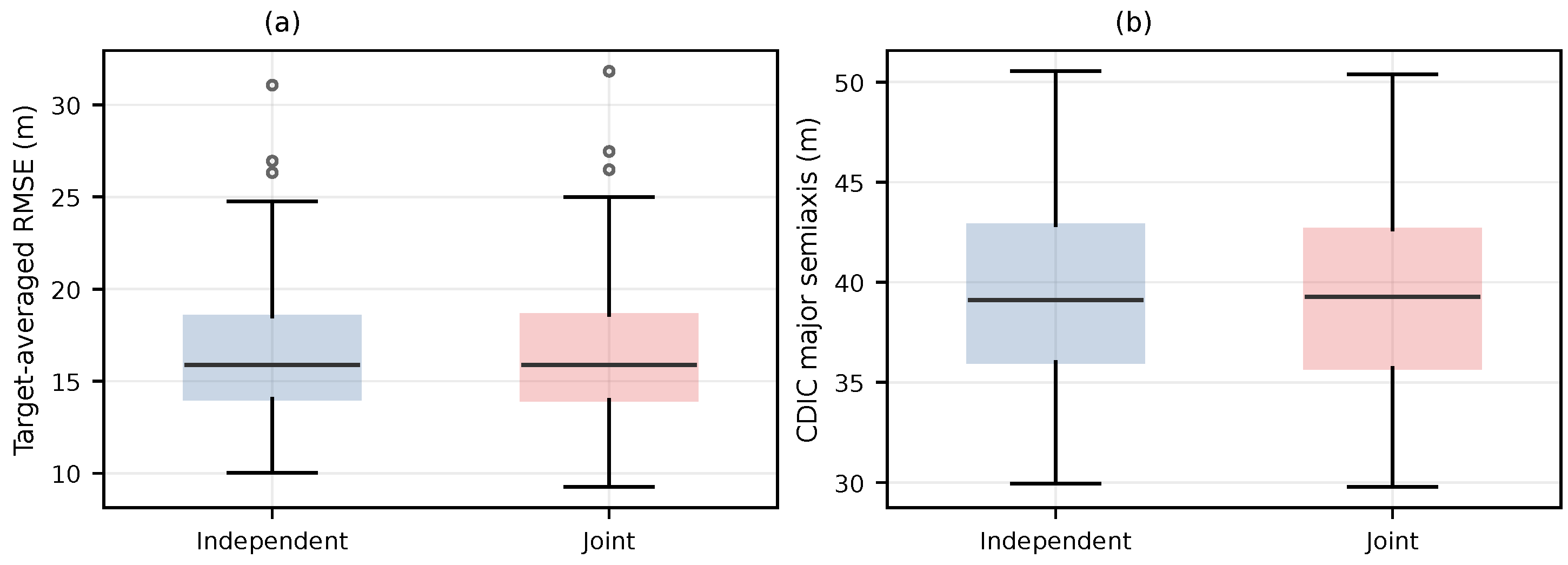
To test transfer beyond the controlled scenarios, a separate experiment generated 128 local-orbital configurations consistent with the dynamics without scenario labels or a prescribed relation topology. Initial relative states, finite-burn parameters, observation-noise scale, chaser acceleration, and parameters of the time-correlated sensor bias were sampled from the prescribed physical ranges. Stochastic target accelerations were generated from positive-semidefinite covariance models permitting both positive and negative cross-correlations. For each sampled scenario, eight stochastic replications were generated, and Independent and Joint SOIR were evaluated using identical truth and observation realizations in each replication. The 10,000 cluster-bootstrap resamples treated configurations as independent units while retaining inner realizations, targets, and prediction times within their parent configuration.

3.2. Comparative Methods

Six methods are evaluated: CV-Q, CA-Q, KF-CV, KF-CA, Independent SOIR, and Joint SOIR. Each method employs the same relative-motion model as follows:
δ x k + 1 B j / A = Φ k rel δ x k B j / A + Γ k rel a k , j rel + w k , j rel , w k , j rel N ( 0 , Q k , j orb ) ,
where Φ k rel and Γ k rel are derived from the same relative-orbit dynamics employed by SOIR. CV-Q represents unresolved acceleration through process covariance, whereas CA-Q augments the state with a persistent relative acceleration. For model r { CV , CA } , let λ r > 0 denote the process-noise scale and let L r denote the predefined candidate set used for history-only calibration:
Q k CV ( λ CV ) = Q k orb + Γ k rel Σ a , k ( λ CV ) ( Γ k rel ) T , y k CA = ( δ x k B j / A ) T ( a k , j rel ) T T , y k + 1 CA = Φ k rel Γ k rel 0 I 3 y k CA + w k CA , w k CA N 0 , Q k CA ( λ CA ) .
The matrix Σ a , k ( λ CV ) S + 3 is the discrete acceleration covariance, and Q k CA ( λ CA ) S + 9 is the augmented covariance associated with the persistent-acceleration model. Both discrete covariances are derived from the orbital transition and continuous white-noise discretization used throughout the implementation.
KF-CV and KF-CA apply the standard Kalman recursion to the CV and CA orbital models, respectively. The following equations suppress the target index j. For a candidate λ L r , the history innovation and corresponding covariance are defined by the following [26,33]:
ν k r , λ = z k H k r μ k k 1 r , λ , S k r , λ = H k r P k k 1 r , λ ( H k r ) T + R k e ,
where H k r is the relative-position measurement matrix for model r. The history-only scale minimizes the summed Gaussian innovation negative log likelihood,
λ r = arg min λ L r k K i 0 K z ( ν k r , λ ) T ( S k r , λ ) 1 ν k r , λ + log det S k r , λ + n z log ( 2 π ) .
The set K z contains the epochs with available measurements. The selected scale λ r is held fixed during future propagation; neither future truth nor coverage statistics enter selection of λ r .
Independent SOIR solves one chaser–target graph per object and removes the cross-target paths. Joint SOIR retains one shared chaser chain and the pair factors supported by the available history. The two SOIR branches otherwise use identical local dynamics, equivalent-maneuver and event factors, priors, measurements, CDIC mapping, and common-random-number realizations. Consequently, the comparison isolates the information architecture rather than a change in the dynamics or likelihood model.
Existing behavior- and intention-recognition methods were discussed qualitatively but were not included as numerical baselines. Those methods primarily produce maneuver classes, intention labels, or predicted trajectories, whereas the present study evaluates probabilistic reachable regions for each target in terms of coverage, prediction-center RMSE, and region size. A consistent numerical comparison would require converting the cited methods into predictors that output calibrated probabilistic regions and is therefore left for future work.

3.3. Evaluation Metrics

For target B j , Monte Carlo realization m { 1 , , M } , and future query t k , let μ ρ , m , k B j and P ρ , m , k B j be the predicted CDIC center and covariance. Let K j , m be the valid future-query index set, define the terminal-query index as k f , j , m : = max K j , m , and set N : = m = 1 M j = 1 N B | K j , m | . The membership indicator matched by target, Monte Carlo run, and time is defined as follows:
I j , m , k = I ρ m , k B j , true E j , m , k CDIC ( α ) .
Every reported target–run pair has a nonempty query set. Therefore, k f , j , m is defined, and the N B M denominators below contain exactly the reported target–run pairs. Aggregating the indicators gives point coverage, per-target all-query coverage, and terminal coverage.
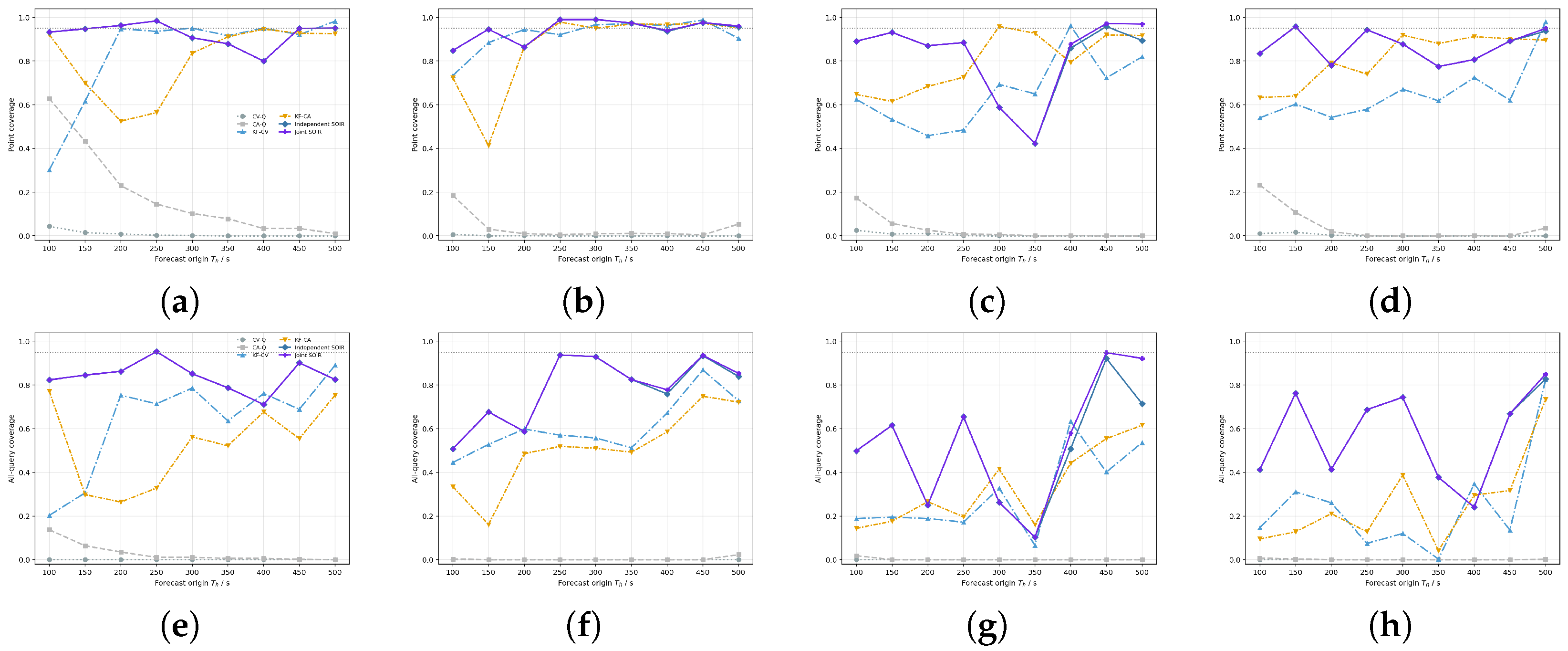
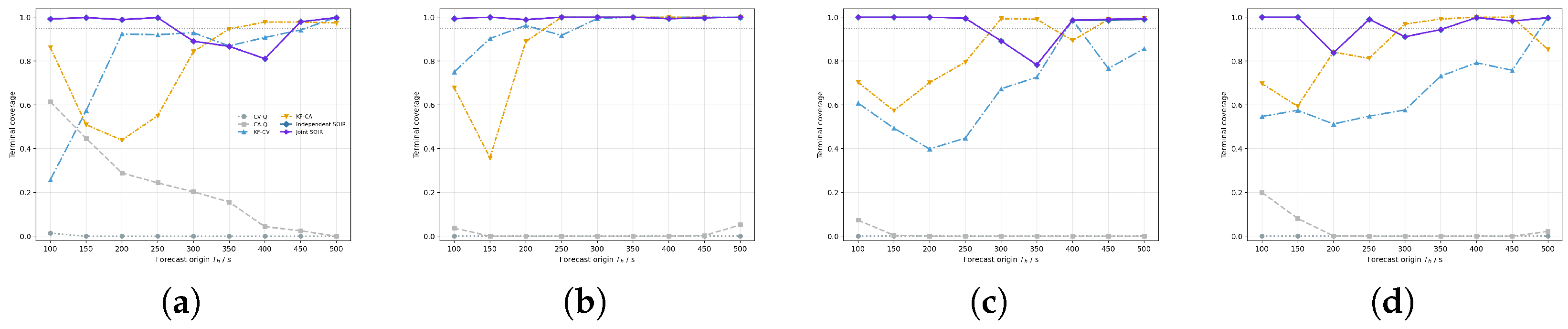
C pt = 1 N m = 1 M j = 1 N B k K j , m I j , m , k , C tr = 1 N B M m = 1 M j = 1 N B k K j , m I j , m , k , C f = 1 N B M m = 1 M j = 1 N B I j , m , k f , j , m .
C pt , C tr , and C f are empirical truth-coverage frequencies for E CDIC : pooled pointwise, per-target all-query, and terminal-query coverage, respectively. For C tr , each target is evaluated separately in each Monte Carlo run; a target–run sample is counted as covered only if its CDIC ellipsoid contains the corresponding true position at every queried prediction time. These quantities evaluate E CDIC , rather than the complete region R CDIC . Prediction-center error and ellipsoid size are defined next.
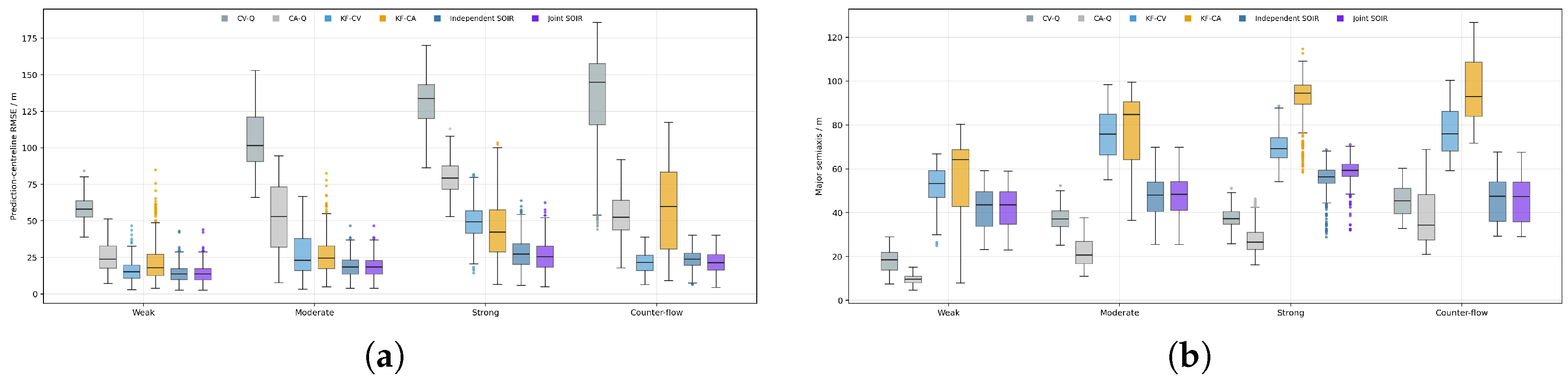
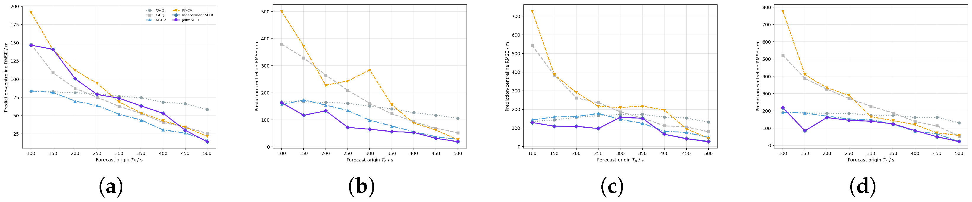
RMSE j , m = 1 | K j , m | k K j , m ρ m , k B j , true μ ρ , m , k B j 2 2 , a j , m , k max = χ 3 2 ( α ) λ max ( P ρ , m , k B j ) , RMSE ¯ = 1 N B M m = 1 M j = 1 N B RMSE j , m , a ¯ max = 1 N m = 1 M j = 1 N B k K j , m a j , m , k max .
Table 4 retains the manuscript definition of RMSE ¯ , evaluated from 640 target–run trajectory RMSE values for each scenario and method. To quantify Monte Carlo precision for each method without treating the four targets as independent replicates, let Y m ( a , q ) be the within-run aggregate of metric q for method a. For the RMSE column of Table 4,
Y m ( a , RMSE ) = 1 N B j = 1 N B RMSE j , m ( a ) , Y ¯ ( a , q ) = 1 M m = 1 M Y m ( a , q ) , MCSE ^ Y ¯ ( a , q ) = s q ( a ) M , M = 160 .
where s q ( a ) is the sample standard deviation of the 160 run-level values. Table 4 reports Y ¯ ( a , q ) and the run-level normal-approximation interval Y ¯ ( a , q ) ± 1.959964 MCSE ^ ( Y ¯ ( a , q ) ) ; coverage endpoints are truncated to [ 0 , 1 ] . The complete run, rather than an individual target or query, is the independent unit.
The Monte Carlo sequence through the adopted M = 160 runs showed stable point estimates and the expected M 1 / 2 reduction in confidence-interval half-width. Additional runs would primarily narrow the intervals; within the observed precision, the method comparisons and qualitative conclusions remained stable.
Each posterior covariance is decomposed as P ρ , m , k B j = V diag ( λ 1 , λ 2 , λ 3 ) V T to construct the three-dimensional wireframe. The ellipsoid is centered at μ ρ , m , k B j , the columns of V define the principal directions, and a q = χ 3 2 ( α ) λ q gives the semiaxis lengths for q = 1 , 2 , 3 . One ellipsoid is drawn for every valid target–time query. All panels use the coordinates in the exported orbital frame and native semiaxis lengths, so the visual differences preserve estimator-induced changes in center and covariance.

3.4. Three-Dimensional Scenario and Reachable Envelope

Figure 2 first shows the geometries of the four scenarios together with the target-indexed sequence of posterior CDIC regions. Figure 3 then resolves the matched Independent/Joint comparison for the Strong and Counterflow scenarios at the primary forecast origin. Each panel uses the same truth trajectory, query times, probability level, and physical-coordinate limits for the corresponding target pair.
The global and target-wise views are descriptive counterparts of the target-matched coverage, RMSE, and major-semiaxis statistics below rather than independent performance measures.

3.5. Coverage and Prediction Error

All six methods produce position regions parameterized by each target covariance and are therefore evaluated within the same set class. For SOIR, the reported coverage and compactness statistics refer to the posterior ellipsoid E CDIC ; residual maneuver support and geometric dilation are excluded.
The effect of cross-target coupling depends on the operating regime and the evaluation metric. Table 4 reports a separate run-level Monte Carlo interval for every method while retaining the original RMSE estimand. The two SOIR estimators yield nearly identical values for the reported metrics in Weak. In Moderate, Joint increases point and all-query coverage by 0.43 and 1.40 percentage points, respectively, with nearly unchanged target-averaged RMSE and a 0.44 m increase in mean major semiaxis. Strong shows the largest differences favoring Joint: point and all-query coverage increase by 7.50 and 20.78 percentage points, and target-averaged RMSE decreases by 1.55 m , while the mean major semiaxis increases by 3.35 m . Counterflow exhibits a different trade-off: point and all-query coverage increase by 1.25 and 2.19 percentage points, target-averaged RMSE decreases by 2.02 m , and the mean major semiaxis decreases by 0.12 m .
Across the four scenario averages, Joint matches or improves Independent in coverage and prediction-center error, with a larger mean region in Moderate and Strong. These averages do not imply uniform improvement across individual realizations because Section 3.6.3 contains both favorable and unfavorable paired changes. In Counterflow, KF-CV has approximately 3.06 percentage points higher point coverage than Joint SOIR but a 31.89 m larger mean major semiaxis; the corresponding RMSE values are 21.44 m for KF-CV and 21.68 m for Joint SOIR. Joint therefore uses cross-target information only when supported by the observed history; it is not a uniformly superior replacement for Independent SOIR. These comparisons are limited to the tested scenarios, histories, methods, and metrics (Figure 4 and Figure 5).
Residual-support calibration was conducted separately from empirical coverage of E CDIC . For each of the 64 fixed history–target–query cells in the Moderate and Strong scenarios, N η = 10 , 000 conditional trajectories were generated under the independent-residual baseline. One-sided 95% Clopper–Pearson lower bounds were Bonferroni-adjusted over the full 256-cell family, including the supplementary dependence conditions. Across the 64 baseline cells, p ^ η , c ranged from 0 to 0.9287 , β ^ η , c L from 0 to 0.919147 , and the induced Fréchet–Hoeffding lower bound from 0 to 0.869147 . A zero lower endpoint does not imply zero empirical coverage; it provides no positive lower bound for that cell. Consequently, the calibration establishes no positive uniform complete-CDIC guarantee. The complete cell-level values and the calibration protocol are provided in the supplementary archive.

3.6. Sensitivity and Generalization

The following analyses examine the coupled history–forecast allocation, robustness to selected calibration values, and performance beyond the four constructed scenarios.

3.6.1. History–Forecast Allocation

Altering T h while retaining the common endpoint changes both the available history and the prediction duration T p = T f T h . Figure 6, Figure 7, Figure 8 and Figure 9 therefore describe a coupled history–forecast allocation rather than an isolated history-length test.
At early forecast origins, the relation factors are inactive or produce negligible differences between the two estimators because the available histories provide insufficient relation evidence. At the primary forecast origin, the Strong and Counterflow histories activate coupled inference. The resulting differences become apparent in coverage and prediction-center RMSE while the region scales remain comparable. The nonmonotone trend is consistent with the combined effects of evidence accumulation and a shortening prediction horizon.

3.6.2. Sensitivity of Selected Calibration Parameters

Figure 10 summarizes the primary threshold experiment. In Strong, increasing κ min from the nominal value of 0.25 to 0.50 reduced the mean number of admitted pair relations from 4.55 to 1.70 . Joint RMSE increased from 25.891 to 26.275 m , whereas point coverage changed from 0.96953 to 0.96797 . The RMSE reduction relative to Independent decreased from 1.599 to 1.215 m but did not reverse. The group-coupling branch was not activated in Weak, whereas Counterflow retained the validated persistent-pair branch. Thus, κ min controls relation admission rather than maneuver-event activation.
The supplementary analyses assess the Joint–Independent comparison over the prespecified parameter ranges. Joint retained a lower mean RMSE than Independent throughout the examined c ev , κ η , and τ cov ranges in Strong and Counterflow, although the magnitudes of the RMSE and region-size differences varied. Consistent with its covariance-memory role, τ cov affected the major-semiaxis difference but not the mean RMSE in the reported formulation. When no candidate relation was admitted, Joint coincided with Independent. These results support local robustness around the nominal calibration values; the complete numerical ranges are provided in the supplementary archive. The earlier relation-mismatch tests used 12 runs with matched random inputs and are retained only as a mechanism diagnostic, not as evidence of a general performance advantage.

3.6.3. Evaluation Under Randomized Dynamics-Consistent Scenarios

To examine performance beyond the four constructed scenarios, we generated 128 four-target realizations by sampling the initial states, maneuver parameters, and observation conditions from continuous distributions subject to the prescribed physical and dynamical constraints. Each scenario realization was evaluated using eight matched seed-indexed realizations shared by Independent and Joint. Table 5 summarizes the scenario-level results, and Figure A1 in Appendix B shows the corresponding distributions. On average, Joint reduced target-averaged RMSE by 0.090 m and the mean CDIC major semiaxis by 0.100 m ; the confidence interval for the paired point-coverage difference included zero.
Joint had lower scenario-level RMSE in 72 realizations and higher RMSE in 56. The estimated association between realized historical dependence and the paired RMSE change was weak, and the test did not reject zero association (Spearman ρ S = 0.109 , p = 0.220 ). Within the declared local-orbital simulation domain, Joint produced small average reductions in RMSE and major semiaxis but did not improve every realization. The two estimators therefore remain complementary: Independent provides the baseline when reliable cross-target evidence is absent, whereas Joint can use relations supported by the observed history. The empirical point coverage of approximately 0.92 is neither a frequentist guarantee at level 0.95 nor a simultaneous-coverage statement.

3.7. Additional Robustness and Computational-Scaling Analyses

The fixed-duration comparison separates the effect of history length from prediction duration, the future-maneuver experiment evaluates sensitivity to violations of the future-innovation independence assumption, and the target-number experiment measures computational growth over the tested target counts.

3.7.1. Fixed Prediction-Duration Comparison

Table 6 fixes T p = 100 s and reports the Joint-minus-Independent changes, thereby isolating history length from the prediction duration. This supplementary experiment uses M = 80 runs per scenario. Table 4 provides the separate M = 160 primary comparison at T h = 500 s .
The fixed-duration comparison shows identical metrics for the two estimators at the earliest forecast origin and small, metric-dependent differences at the intermediate origin. Coverage and RMSE differences favoring Joint in Strong and Counterflow appear only after the longer history. Therefore, the primary-origin differences cannot be attributed solely to the shorter prediction interval.

3.7.2. Sensitivity to Correlated Future Maneuvers

In a separate stress test, both CDIC estimators were evaluated with 80 new seeds in each of the Moderate and Strong scenarios. All outcomes were retained, including 70 of 80 Moderate runs and 19 of 80 Strong runs in which no relation was admitted and Joint therefore coincided with Independent. The observed history ends at 500 s, and the four targets are queried at 510, 540, 570, and 600 s. The estimators, covariance calibration, and original controls remain fixed. The added maneuvers are applied only to future target truth trajectories, with identical random draws for each seed across estimators and correlation conditions.
For coordinate axes a , b and s , u = i , , i + 9 , define zero-mean, unit-variance jointly Gaussian latent variables γ j , s , a by
R B = ( 1 ρ B ) I 4 + ρ B 1 4 1 4 T , Cov ( γ j , s , a , γ l , u , b ) = [ R B ] j l ρ T | s u | δ a b .
The four disturbance conditions are I (independent across targets and future epochs), B (between-target correlation only), T (temporal correlation only), and BT (both between-target and temporal correlation). They use ( ρ B , ρ T ) = ( 0 , 0 ) , ( 0.75 , 0 ) , ( 0 , 0.75 ) , ( 0.75 , 0.75 ) , respectively. These upright labels identify disturbance conditions, not the Independent and Joint estimators. The coefficients ρ B and ρ T describe the latent Gaussian variables, not Pearson correlations after transformation. With Φ denoting the standard-normal CDF, define componentwise
u j , s marg = ( η ¯ j | u j , s base | ) + , Δ u j , s = 1 2 u j , s marg [ 2 Φ ( γ j , s ) 1 3 ] , Δ x j , s + 1 = F s B j Δ x j , s + G s B j Δ u j , s , Δ x j , i = 0 .
Δ x R 6 denotes the added state perturbation, and Δ u R 3 denotes the added control perturbation. The added inputs over 500–590 s leave all states and measurements through 500 s, as well as the complete chaser trajectory, unchanged. Conditional on the fixed nominal commands, each added-input marginal has zero mean and variance ( u j , s , a marg ) 2 / 12 , and the total controls satisfy the original componentwise limits. The base commands are not recomputed from the perturbed states. Condition I therefore means independent added perturbations, not an uncorrelated base scenario. Because the perturbations affect only unobserved future truth, the forecast outputs and graph information matrices are identical across the four correlation conditions; this equality was also verified in additional repetitions of the full interface (Table 7).
The largest absolute coverage change across the four bounded perturbation conditions is 0.0032 . Temporal correlation, however, increases Joint RMSE by 1.23 m in Moderate and 0.69 m in Strong (T minus I), with paired 95% bootstrap intervals of [1.03, 1.43] and [0.49, 0.88] m, respectively. Complete paired runs were resampled to form these pointwise intervals; no multiplicity adjustment was applied. The reported frequencies are not Gaussian probability contents. The sensitivity results neither identify future correlations from the observed history nor certify nominal- α coverage under arbitrary disturbance laws.
A complementary numerical verification fixes the boundary Gaussian and transition matrices from the first Joint realization in Strong and generates 5000 paired samples under the same four conditions I , B , T , and BT . Single-epoch marginal variances and independent process noise in the physical dynamics remain unchanged, and the forecast-origin state is independent of future innovations. Across ten forecast steps, the generalized covariance identity agrees with an autoregressive recursion assembled independently to a maximum relative Frobenius error of 5.76 × 10 16 . Between-target correlation preserves target-wise position covariance but changes relative-position covariance, whereas temporal correlation changes target-wise covariance after the two-step propagation delay. Table 8 reports selected diagnostics at 600 s. This verification confirms the covariance calculation under the specified kernel; it neither identifies the future-disturbance law in operation nor validates the main covariance calibration.

3.7.3. Computational Impact of Target Count

The experiment considers N B { 2 , 4 , 8 , 12 , 16 } with ( T h , T p ) = ( 500 , 100 ) s . Each timing trial is executed in a separate process under the fixed level of parallelism stated in Section 3.1. Computational time includes factor-graph assembly, posterior estimation, selected-covariance recovery, and CDIC prediction. Table 9 reports endpoint values and slopes, while Figure A2 in Appendix B shows the measured values. The comparison uses the Independent estimator applied target-wise and Joint without top-k truncation. Joint evaluates all N B 2 candidate relations and retains those satisfying the historical-evidence criterion. Peak resident set size (RSS) measures memory demand.
All 30 timing-and-memory trials and 120 matched accuracy trials completed successfully. Runtime columns in Table 9 report medians from three separately launched trials, and the slopes are log–log fits over the tested range. From N B = 2 to N B = 16 , median end-to-end time increased by factors of 7.2 and 52.3 for Independent and untruncated Joint, respectively. The Joint factor is an increase across target counts, not a Joint-to-Independent runtime ratio. The measured slopes of 0.96 and 1.91 are consistent with the elimination-clique and O ( N B 2 L p ) covariance-propagation costs in Equation (63); they do not constitute an asymptotic proof.
In the separate accuracy experiment with matched inputs at N B = 16 , point-coverage frequencies were 0.9010 for Independent and 0.8997 for Joint. The corresponding RMSE values were 31.15 and 31.22 m , and the mean CDIC major semiaxes were 56.70 and 56.65 m . The absolute differences were therefore 0.0013 , 0.07 m , and 0.05 m , respectively.

4. Conclusions

This study develops a joint local Markov factor graph for predicting the probabilistic future occupied regions of multiple non-cooperative space objects based on relative measurements. The formulation estimates the shared chaser and augmented target trajectories and equivalent maneuvers in a single sparse posterior, using target relations supported by the observed history. Schur complement marginalization characterizes the cross-target dependence resulting from the shared chaser state, and dynamics-consistent propagation maps the resultant target marginals to time-indexed CDIC regions.
The formal analysis identifies the direct and shared-state contributions to cross-target dependence and establishes a sufficient vanishing-coupling condition under which the Joint posterior factorizes by target. Exact agreement with separately constructed target-wise posteriors also requires matched diagonal information pairs. The analysis also establishes the sharp dependence-free Fréchet–Hoeffding lower bound for target-wise CDIC containment and a conservative outer-ellipsoid inclusion that does not define an exact joint probability region.
Monte Carlo simulations demonstrate the proposed method’s ability to jointly estimate target states and equivalent maneuvers based on finite measurement histories of non-cooperative objects and propagate the resulting posterior into target- and time-indexed probabilistic reachable regions. These regions represent target motion tendencies in a continuous probabilistic form and provide state and uncertainty information for subsequent behavior analysis and intent inference. In Strong, Joint increased point and all-query coverage by 0.0750 and 0.2078 , respectively, and reduced target-averaged RMSE by 1.55 m , with a 3.35 m increase in mean major semiaxis. Randomized scenarios contained both favorable and unfavorable paired changes, so the two estimators are treated as complementary rather than uniformly ranked.
Nonetheless, the present validation assumes known target identities, a calibrated relative-position likelihood, and predominantly unimodal future motion. The residual-support level remains a modeling assumption. Under the independent-residual calibration, its simultaneously adjusted one-sided lower confidence bound ranged from 0 to 0.919147 across the tested cells; consequently, the experiment established no positive uniform complete-CDIC lower bound. Extending the framework to missed detections, association uncertainty, multimodal maneuvers, and closed-loop collision avoidance requires dedicated measurement and decision models. Future work will examine these extensions and assess the additional set-valued support terms of the CDIC construction under mission-informed disturbance laws.

Author Contributions

Conceptualization, T.M. and S.L.; methodology, T.M.; software, T.M.; validation, T.M., B.N. and M.S.; formal analysis, T.M. and B.N.; writing—original draft preparation, T.M.; writing—review and editing, T.M., B.N., M.S. and S.L.; supervision, S.L. All authors have read and agreed to the published version of the manuscript.

Funding

This research received no external funding.

Data Availability Statement

The datasets presented in this article are not readily available because the datasets are part of an ongoing study. Requests to access the datasets should be directed to the corresponding author.

Conflicts of Interest

The authors declare no conflicts of interest.

Nomenclature

A, B j , N B Chaser, the jth non-cooperative target, and the number of targets.
O Local orbital frame.
Δ t ; L h , L p ; T h , T p Sampling interval; history and prediction lengths; corresponding time durations.
L b , L c Behavior-evidence and coupling-score averaging lengths.
x k q , y k B j Physical state of object q and augmented target state.
ρ k q , v k q , η k B j Position, velocity, and equivalent target maneuver state.
u k A Known chaser control input conditioned on in the posterior.
z k , j , h k , j ( · ) , n z Supplied relative-position measurement, state measurement function, and measurement dimension.
R k , j e , Ω k , j z Effective measurement covariance and corresponding information matrix.
m j , k b , e j , k , e ˜ j , k , e ¯ j , k Target behavior summary, unconstrained event coordinate, bounded covariance argument, and logistic evidence target.
κ e , g e , θ e , c ev Event persistence, logistic gain, normalized event threshold, and event-dependent covariance-increment ratio.
sigm ( · ) , clip [ 0 , 1 ] ( · ) , ( · ) + Logistic sigmoid, interval-clipping, and positive-part operators.
col ( · ) Vertical concatenation in lexicographic index order.
κ η , ρ cov ( δ t ) , τ cov Latent conditional-mean persistence, auxiliary forecast-covariance memory law, and covariance-memory time constant.
F k q , G k q , A k η , j Physical transition, input injection, and augmented target transition matrices.
K i c , κ j l , i , κ min Sparse coupling matrix, target pair coefficient, and global group-edge threshold.
( · ) ^ h Measurement-conditioned history estimate fixed before active pair-factor assembly.
η j , i h , avg , η ¯ j History-averaged equivalent-maneuver estimate and physical componentwise maneuver bound, respectively.
Δ ρ j l , k , Δ m j l , k b Target-pair relative-position and behavior differences.
Ψ i entry , Θ ¯ i , k 0 entry , P i , k 0 entry Configured window-entry information potential, mean, and covariance for one batch solve.
ϕ k , j pred Direct augmented-dynamics transition factor for future target states.
ϕ ζ , r ζ , Θ ζ Local factor, corresponding residual, and connected local variable block.
Λ i , ξ i Linearized posterior information matrix and information vector.
L i , w i , m i Unwhitened full-column-rank entry-and-transition operator, information-block eigenvalue lower bound, and resulting eigenvalue lower bound.
S B , S sh Boolean selectors for aggregate target and shared-chaser blocks.
P Θ , i , P B m Active-state covariance and aggregate marginalized target block.
y ˇ i + τ B j Future augmented target state generated by the prediction transition kernel.
μ ρ , i + τ B j , P ρ , i + τ B j Predicted target position mean and covariance.
Π j , τ ρ , Q j l υ ( s , u ) Target position-moment propagation map and specified future innovation cross-covariance block.
P j l , k i B , 0 , P j l , k i B , Q Cross-target predicted covariance with zero off-diagonal future innovation blocks and with the specified future cross-innovation kernel, respectively.
μ η , j , s i , P η , j , s i Time-propagated equivalent maneuver mean and covariance.
ς η , j , s p ( α η ) , b η , j , s Componentwise covariance allowance and the remaining residual physical budget.
α , α η , β η Local-Gaussian content, maneuver-support allocation level, and assumed residual-event probability lower bound.
q j , τ , P q , η , A G , A η Local Gaussian position law, joint predictive measure, posterior-error event, and residual-support event.
ρ B , ρ T , R B , δ a b Between-target and temporal correlation coefficients, target-correlation matrix, and Kronecker delta used in the future-maneuver stress kernel.
γ j , s , u j , s base , u j , s marg Standard-Gaussian stress variable, fixed baseline command, and available componentwise command margin.
Δ u j , s , Δ x j , s , ν s , j η Added bounded command, resulting state perturbation, and Gaussian maneuver innovation.
I Disturbance condition independent across targets and future epochs: ( ρ B , ρ T ) = ( 0 , 0 ) .
B Between-target correlation only: ( ρ B , ρ T ) = ( 0.75 , 0 ) .
T Temporal correlation only: ( ρ B , ρ T ) = ( 0 , 0.75 ) .
BT Combined between-target and temporal correlation: ( ρ B , ρ T ) = ( 0.75 , 0.75 ) .
r tr Ratio of covariance traces under the specified and independent innovation kernels.
ρ i + τ B j , occ Physical point occupied by target B j after residual-maneuver and geometric-dilation effects.
E j , i + τ CDIC Posterior position region used by the CDIC construction.
Δ U η , j , s , C j , i i + τ η Residual maneuver-support box and corresponding propagated position support.
R j , i + τ CDIC Complete target-wise CDIC region including residual support and dilation.
T , R j , i CDIC , O i S Discrete prediction-time set, target time tube, and multi-target scene time tube.
i, r, s it , LM Forecast-origin index, outer configuration-refresh index, inner nonlinear-iteration index, and LM trial index.
c i ( r ) , G i Fixed inner-solve configuration and the interval-clipping-and-evidence refresh map.
S i , T i , ω Exact conditional solution map and under-relaxed configuration fixed-point map.
L S , i , L G , i , L T , i , ω , δ r Conditional-solve, refresh, and fixed-point Lipschitz bounds, and finite-inner-solve refresh error bound.
f i ( s it ) , J i ( s it ) , H i ( s it ) , g i ( s it ) Whitened residual, residual Jacobian, Gauss–Newton matrix, and gradient vector.
A i , b i , H i , h i Final active-branch affine system, normal matrix, and normal-equation right-hand side.
r NE , i Scaled final normal-equation residual.
λ s it , LM , λ 0 , λ lo , λ hi , β λ LM trial damping, initial value, lower and upper bounds, and damping multiplier.
ρ s it , LM , ρ min LM model-agreement ratio and acceptance threshold.
ε Θ , ε J , N it , ε abs , ε NE , ε GN Inner stopping tolerances and cap, absolute objective allowance, final normal-equation tolerance, and GN objective margin.
r out , i ( r ) , ε out , ω , N out Outer consistency residual, tolerance, under-relaxation coefficient, and refresh cap.
Λ ¯ i , ε cov , D i Retained covariance-information interface, additive coefficient, and scaling matrix; the reported setting is listed in Results.
D i n , B i Diagonal equilibration matrix and balanced retained information matrix; the reported path is undamped and unregularized.
d c Maximum active pair degree.
C c , Q i Elimination clique and requested covariance-block set.
M, Y m ( a , q ) , s q ( a ) Number of independent Monte Carlo runs, method-specific within-run aggregate, and run-level sample standard deviation.
C pt , C tr , C f Point, all-query, and terminal empirical coverage metrics.
RMSE ¯ , a ¯ max Target-averaged trajectory RMSE and mean major semiaxis.
N η , c, p ^ η , c Number of conditional residual trajectories per calibration cell, cell index, and empirical residual-support frequency.
β ^ η , c L Simultaneously adjusted one-sided residual-support lower confidence bound.

Abbreviations

AbbreviationDefinition
SOIRSpace-object inference and reachability.
CDICCorrected-dynamics inferred-control envelope.
MAPMaximum a posteriori estimation.
GPGaussian process.
IMMInteracting multiple model.
KF–CV, KF–CAKalman filters using nominal and maneuver-augmented orbital transitions.
CV–Q, CA–QOpen-loop orbital propagation without and with a persistent acceleration state.

Appendix A. Optional Outer-Ellipsoid Approximation of the CDIC Minkowski Sum

For downstream set computations, the CDIC Minkowski sum in Equation (43) admits the following conservative outer ellipsoid. The construction uses standard support-function results and ellipsoidal calculus for Minkowski sums [34,35]. Define
L j , τ , s = S ρ y Φ j , i + τ : s + 1 B G s B j 0 n η × n η .
Assumption A1
(Positive outer-cover weights). The support weights satisfy ϑ s > 0 and s = i i + τ 1 ϑ s = 1 , while the component weights satisfy ω ρ , ω η , ω dil > 0 and ω ρ + ω η + ω dil = 1 . Degenerate ellipsoidal components are interpreted on their image subspaces.
Let Q ρ , j , i + τ = χ 3 2 ( α ) P ρ , i + τ B j . For a vector b , the notation b 2 denotes componentwise squaring. Define
Q η , j , i + τ = s = i i + τ 1 n η ϑ s L j , τ , s diag ( b η , j , s 2 ) L j , τ , s T .
For Q 0 , define the possibly degenerate ellipsoid by E ( μ , Q ) = { ζ : ζ μ Range ( Q ) , ( ζ μ ) T Q ( ζ μ ) 1 } , where Q is the Moore–Penrose pseudoinverse. For any compact convex set X , define its support function by h X ( u ) : = sup x X u T x .
Proposition A1
(Conservative CDIC outer ellipsoid). Under Assumption A1, the propagated residual support and the CDIC region satisfy
C j , i i + τ η E ( 0 , Q η , j , i + τ ) ,
and
R j , i + τ CDIC ( α ) E μ ρ , i + τ B j , Q j , i + τ o , Q j , i + τ o = Q ρ , j , i + τ ω ρ + Q η , j , i + τ ω η + r dil , j 2 I 3 ω dil .
Proof. 
For each s, every δ η s Δ U η , j , s satisfies
a : b η , j , s , a > 0 δ η s , a 2 n η b η , j , s , a 2 1 ,
because each summand is no larger than 1 / n η ; zero-width coordinates are fixed at zero. Thus
Δ U η , j , s E 0 , n η diag ( b η , j , s 2 ) .
Applying the linear map L j , τ , s gives the possibly degenerate shape
Q s = n η L j , τ , s diag ( b η , j , s 2 ) L j , τ , s T .
For a centered ellipsoid, h E ( 0 , Q ) ( u ) = u T Q u . The support function of the propagated Minkowski sum therefore obeys
h C j , i i + τ η ( u ) s u T Q s u u T s Q s ϑ s u = u T Q η , j , i + τ u ,
where the second line follows from weighted Cauchy–Schwarz. This proves Equation (A3).
After subtracting the common center μ ρ , i + τ B j from both sets, define the dilation shape Q dil = r dil , j 2 I 3 . Applying the same support-function argument with weights ω ρ , ω η , ω dil yields
u T Q ρ , j , i + τ u + u T Q η , j , i + τ u + u T Q dil u 2 u T Q ρ , j , i + τ ω ρ + Q η , j , i + τ ω η + Q dil ω dil u = u T Q j , i + τ o u .
All sets involved are compact and convex. The support function of the CDIC Minkowski sum is therefore no larger than that of the stated ellipsoid in every direction, and compact-convex support-function ordering proves Equation (A4). □
Remark A1
(Probability interpretation of the outer approximation). The outer ellipsoid preserves the lower containment guarantee of Proposition 1 because it contains the original CDIC set. The converse is not implied: the approximation can add points and therefore is not itself an exact α-level posterior region.
A missing component and its weight are removed before the remaining weights are normalized. The weights may be chosen by minimizing log det Q j , i + τ o or tr Q j , i + τ o , depending on the selected compactness criterion.

Appendix B. Supplementary Random-Population and Scaling Evidence

Appendix B.1. Random-Configuration Diagnostics

All propagation outcomes from the 128 configurations were retained, and every initial configuration satisfied the prescribed geometric constraints. Over the full propagation interval, 99.9724% of truth points indexed by target and time remained within the declared 20–1200 m target–chaser band; the few diagnostic excursions were not removed. No target–target safety-distance guarantee is claimed.
Figure A1. Configuration-level distributions over the 128 randomized, local-orbital configurations consistent with the dynamics: (a) target-averaged prediction-center RMSE and (b) mean CDIC major semiaxis. Boxes show medians and interquartile ranges, and whiskers use the 1.5 -IQR rule. Point-coverage results are reported in Table 5.
Mathematics 14 03383 g0a1

Appendix B.2. Resource Scaling with Target Count

The untruncated Joint profile evaluates all N B 2 candidate relations and applies only the historical-evidence criterion. The admitted relation counts for N B = 2 , 4 , 8 , 12 , 16 were 1, 6, 25, 54, and 98, respectively; no fixed edge-number or average-degree cap was imposed.
Figure A2. Resource use over N B = 2 , 4 , 8 , 12 , 16 : (a) measured runtime and (b) peak resident set size (RSS). Runtime bands are interquartile ranges of timing repetitions launched separately, not Monte Carlo confidence intervals.
Mathematics 14 03383 g0a2

References

  1. Clohessy, W.H.; Wiltshire, R.S. Terminal guidance system for satellite rendezvous. J. Aerosp. Sci. 1960, 27, 653–658. [Google Scholar] [CrossRef] [Scilit]
  2. Yamanaka, K.; Ankersen, F. New state transition matrix for relative motion on an arbitrary elliptical orbit. J. Guid. Control Dyn. 2002, 25, 60–66. [Google Scholar] [CrossRef] [Scilit] [PubMed]
  3. Kschischang, F.R.; Frey, B.J.; Loeliger, H.A. Factor graphs and the sum-product algorithm. IEEE Trans. Inf. Theory 2001, 47, 498–519. [Google Scholar] [CrossRef] [Scilit]
  4. Kaess, M.; Johannsson, H.; Roberts, R.; Ila, V.; Leonard, J.J.; Dellaert, F. iSAM2: Incremental smoothing and mapping using the Bayes tree. Int. J. Robot. Res. 2012, 31, 216–235. [Google Scholar] [CrossRef] [Scilit]
  5. Barfoot, T.D.; Tong, C.H.; Särkkä, S. Batch continuous-time trajectory estimation as exactly sparse Gaussian process regression. In Proceedings of the Robotics: Science and Systems X, Berkeley, CA, USA, 12–16 July 2014. [Google Scholar] [CrossRef] [Scilit]
  6. Mukadam, M.; Dong, J.; Dellaert, F.; Boots, B. STEAP: Simultaneous trajectory estimation and planning. Auton. Robot. 2019, 43, 415–434. [Google Scholar] [CrossRef] [Scilit]
  7. King-Smith, M.; Tsiotras, P.; Dellaert, F. Simultaneous control and trajectory estimation for collision avoidance of autonomous robotic spacecraft systems. In Proceedings of the 2022 IEEE International Conference on Robotics and Automation, Philadelphia, PA, USA, 23–27 May 2022; IEEE: New York, NY, USA, 2022; pp. 257–264. [Google Scholar] [CrossRef] [Scilit]
  8. Zhang, H.; Luo, J.; Gao, Y.; Ma, W. An intention inference method for the space non-cooperative target based on BiGRU-Self Attention. Adv. Space Res. 2023, 72, 1815–1828. [Google Scholar] [CrossRef] [Scilit]
  9. Sun, Q.; Zhao, L.; Tang, S.; Dang, Z. Orbital motion intention recognition for space non-cooperative targets based on incomplete time series data. Aerosp. Sci. Technol. 2025, 158, 109912. [Google Scholar] [CrossRef] [Scilit]
  10. Sun, Q.; Zhao, L.; Dang, Z. BiGAT: A model for recognizing motion intentions of space noncooperative targets. IEEE Trans. Aerosp. Electron. Syst. 2025, 61, 2586–2600. [Google Scholar] [CrossRef] [Scilit]
  11. Chen, Y.; Zhang, X.; Liao, W.; Wei, G.; Fan, S. Orbital behavior intention recognition for space non-cooperative targets under multiple constraints. Aerospace 2025, 12, 520. [Google Scholar] [CrossRef] [Scilit]
  12. Yu, Y.; Guo, Y.; Wang, P.; Zhang, H. Intention recognition for space non-cooperative targets using Kolmogorov–Arnold transformer. Aerosp. Sci. Technol. 2026, 170, 111497. [Google Scholar] [CrossRef] [Scilit]
  13. Wang, H.; Zhang, Y.; Bi, S. Game strategy prediction for spacecraft orbital pursuit–evasion game based on long short-term memory. Space Sci. Technol. 2025, 5, 0279. [Google Scholar] [CrossRef] [Scilit]
  14. Zhang, H.; Zhang, J.; Zhang, Z.; Ru, X.; Shen, M. Intention inference for spacecraft proximity maneuver using a cascaded neural network. Aerosp. Sci. Technol. 2026, 168, 111128. [Google Scholar] [CrossRef] [Scilit]
  15. Lee, S.; Hwang, I. Reachable set computation for spacecraft relative motion with energy-limited low-thrust. Aerosp. Sci. Technol. 2018, 77, 180–188. [Google Scholar] [CrossRef] [Scilit]
  16. Shao, L.; Miao, H.; Hu, R.; Liu, H. Reachable set estimation for spacecraft relative motion based on bang–bang principle. Chin. J. Aeronaut. 2023, 36, 229–240. [Google Scholar] [CrossRef] [Scilit]
  17. Wen, C.; Gurfil, P. Relative reachable domain for spacecraft with initial state uncertainties. J. Guid. Control Dyn. 2016, 39, 462–473. [Google Scholar] [CrossRef] [Scilit]
  18. Wen, C.; Gao, Y.; Shi, H. Three-dimensional relative reachable domain with initial state uncertainty in Gaussian distribution. Proc. Inst. Mech. Eng. Part G J. Aerosp. Eng. 2019, 233, 1555–1570. [Google Scholar] [CrossRef] [Scilit]
  19. Wen, C.; Ma, J. Reachable domain for satellite relative motion along elliptic orbit with uncertainty and process noise. Proc. Inst. Mech. Eng. Part G J. Aerosp. Eng. 2020, 234, 1287–1300. [Google Scholar] [CrossRef] [Scilit]
  20. Kousik, S.; Dai, A.; Gao, G.X. Ellipsotopes: Uniting ellipsoids and zonotopes for reachability analysis and fault detection. IEEE Trans. Autom. Control 2023, 68, 3440–3452. [Google Scholar] [CrossRef] [Scilit]
  21. Montenbruck, O.; Gill, E. Satellite Orbits: Models, Methods, and Applications; Springer: Berlin/Heidelberg, Germany, 2000. [Google Scholar] [CrossRef] [Scilit]
  22. Vallado, D.A. Fundamentals of Astrodynamics and Applications, 4th ed.; Microcosm Press: Hawthorne, CA, USA, 2013. [Google Scholar]
  23. Fehse, W. Automated Rendezvous and Docking of Spacecraft; Cambridge University Press: Cambridge, UK, 2009. [Google Scholar] [CrossRef] [Scilit]
  24. Schaub, H.; Junkins, J.L. Analytical Mechanics of Space Systems, 4th ed.; AIAA: Reston, VA, USA, 2018. [Google Scholar] [CrossRef] [Scilit] [PubMed]
  25. Li, X.R.; Jilkov, V.P. Survey of maneuvering target tracking. Part V: Multiple-model methods. IEEE Trans. Aerosp. Electron. Syst. 2005, 41, 1255–1321. [Google Scholar] [CrossRef] [Scilit]
  26. Crassidis, J.L.; Junkins, J.L. Optimal Estimation of Dynamic Systems, 2nd ed.; CRC Press: Boca Raton, FL, USA, 2011. [Google Scholar] [CrossRef] [Scilit]
  27. Dellaert, F.; Kaess, M. Square root SAM: Simultaneous localization and mapping via square root information smoothing. Int. J. Robot. Res. 2006, 25, 1181–1203. [Google Scholar] [CrossRef] [Scilit]
  28. Kaess, M.; Ranganathan, A.; Dellaert, F. iSAM: Incremental smoothing and mapping. IEEE Trans. Robot. 2008, 24, 1365–1378. [Google Scholar] [CrossRef] [Scilit]
  29. Blom, H.A.P.; Bar-Shalom, Y. The interacting multiple model algorithm for systems with Markovian switching coefficients. IEEE Trans. Autom. Control 1988, 33, 780–783. [Google Scholar] [CrossRef] [Scilit]
  30. Tapley, B.D.; Schutz, B.E.; Born, G.H. Statistical Orbit Determination; Elsevier Academic Press: Burlington, MA, USA, 2004. [Google Scholar] [CrossRef] [Scilit]
  31. Lin, Z.; Bai, Z. Probability Inequalities; Springer: Berlin/Heidelberg, Germany, 2011. [Google Scholar] [CrossRef] [Scilit]
  32. Zhang, F. (Ed.) The Schur Complement and Its Applications; Springer: New York, NY, USA, 2005. [Google Scholar] [CrossRef] [Scilit]
  33. Kalman, R.E. A new approach to linear filtering and prediction problems. J. Basic Eng. 1960, 82, 35–45. [Google Scholar] [CrossRef] [Scilit]
  34. Kurzhanski, A.; Valyi, I. Ellipsoidal Calculus for Estimation and Control; Birkhäuser: Boston, MA, USA, 1997; ISBN 978-0-8176-3699-9. [Google Scholar]
  35. Seeger, A. Calculus rules for combinations of ellipsoids and applications. Bull. Aust. Math. Soc. 1993, 47, 1–12. [Google Scholar] [CrossRef] [Scilit]
Figure 1. Joint SOIR factor graph for the estimation-window interface. The target chains share chaser states and evidence-supported historical interaction paths. The resulting current marginals and cross-covariance blocks are subsequently propagated by the posterior-prediction model.
Mathematics 14 03383 g001
Figure 2. Joint-model time-indexed CDIC reachable envelope sequences: (a) Weak; (b) Moderate; (c) Strong; (d) Counterflow. The blue, orange, green, and red solid lines denote the trajectories of targets B 0 , B 1 , B 2 , and B 3 , respectively.
Mathematics 14 03383 g002
Figure 3. Target-wise matched Independent/Joint CDIC sequences at T h = 500 s : (ad) Strong targets B 0 B 3 and (eh) Counterflow targets B 0 B 3 .
Mathematics 14 03383 g003
Figure 4. T h = 500 s target-matched CDIC point coverage, coverage over all prediction queries, and terminal coverage: (a) Weak; (b) Moderate; (c) Strong; (d) Counterflow. Within each panel, P, A, and F denote point, all-query, and terminal coverage, respectively; bar colors identify the six methods. Error bars show method-specific 95% run-level normal-approximation confidence intervals. The dotted reference line denotes the nominal marginal level α = 0.95 , not an empirical coverage guarantee.
Mathematics 14 03383 g004
Figure 5. T h = 500 s prediction-center RMSE and CDIC major semiaxis distributions: (a) prediction-center RMSE; (b) major semiaxis. Boxes show medians and interquartile ranges; whiskers use the 1.5 -IQR rule. Each box contains 640 target–run samples, and points beyond the whiskers are retained and displayed as outliers. These distributions use target–run samples, whereas the intervals in Table 4 use 160 independent run-level aggregates.
Mathematics 14 03383 g005
Figure 6. Forecast-origin CDIC coverage: (ad) point coverage and (eh) all-query trajectory coverage, in Weak, Moderate, Strong, and Counterflow order. The dotted reference line denotes the nominal marginal level α = 0.95 , not an empirical coverage guarantee.
Mathematics 14 03383 g006
Figure 7. Forecast-origin terminal CDIC coverage: (a) Weak; (b) Moderate; (c) Strong; (d) Counterflow. The dotted reference line denotes the nominal marginal level α = 0.95 , not an empirical coverage guarantee.
Mathematics 14 03383 g007
Figure 8. Forecast-origin prediction-center RMSE: (a) Weak; (b) Moderate; (c) Strong; (d) Counterflow.
Mathematics 14 03383 g008
Figure 9. Forecast-origin CDIC major semiaxis: (a) Weak; (b) Moderate; (c) Strong; (d) Counterflow.
Mathematics 14 03383 g009
Figure 10. Sensitivity to the group-edge admission threshold. Curves show means from 80 matched realizations indexed by seed, with 95% intervals (Student t for the scans and normal approximation for the Independent references) at each parameter value. The realizations are shared across methods and threshold values. The dashed line marks the prespecified value κ min = 0.25 . Panel (a) reports group-mode activation, and panel (b) compares Joint RMSE with the corresponding Independent reference. Colors identify scenarios; solid curves denote Joint and dotted curves denote Independent.
Mathematics 14 03383 g010
Table 1. Shared physical, stochastic, and inference settings.
SymbolValueUnitSymbolValueUnit
N B , M 4 , 160 ( n x , n η , n z ) ( 6 , 3 , 3 )
n ref 1.027 × 10 3 rad · s 1 T f , T h , T p 600 , 100 : 50 : 500 , T f T h s
Δ t , Δ t z 10 , 10 s L b , L c 2 , 2
α 0.95 χ 3 2 ( α ) 7.815
κ η 0.74 τ cov 50 s
β 1 / ( L b + 1 ) e j , 0 0
a A max , a B max 0.008325 , 0.009143 m · s 2 r geom , r safe 2.5 , 5.0 m
σ η , rw 0.00145 m · s 2 σ η , E , σ η , lim 0.0042 , 0.0032 m · s 2
c ev 1.5 κ e , g e , θ e 0.82 , 1.6 , 2.0
σ e , d , σ e , z 0.20 , 0.16 w ρ , w v , w , w η 0.25 , 0.25 , 0.15 , 0.35
σ ρ 260 m σ v 1.20 m · s 1
σ 0.55 σ η 0.0040 m · s 2
σ pair , ρ 90 m σ pair , m 0.0040 m · s 2
κ min 0.25 dim ( r k , j l pair ) 6
Table 2. Initial truth states for the four controlled scenarios. Exported target identifiers B 0 B 3 correspond to model indices j = 1 –4.
SceneObject ρ x / m ρ y / m ρ z / m v x / ( m · s 1 ) v y / ( m · s 1 ) v z / ( m · s 1 )
WeakA 180 95150 0.0550 0.0200 0.0140
B 0 803618 0.3690 0.1656 0.0684
B 1 82 34 16 0.3780 0.1566 0.0612
B 2 55 62 20 0.2700 0.3024 0.0756
B 3 58 58 18 0.2952 0.2952 0.0684
ModerateA 180 95150 0.0550 0.0200 0.0140
B 0 924218 0.7560 0.3420 0.0810
B 1 94 36 16 0.7650 0.2970 0.0720
B 2 62 76 20 0.5490 0.6750 0.0900
B 3 68 70 18 0.5940 0.6570 0.0810
StrongA 215 105260 0.0850 0.0450 0.0260
B 0 136 74 34 0.3600 0.4590 0.0828
B 1 132 70 32 0.9270 0.4230 0.0756
B 2 1169436 0.8010 0.3330 0.0828
B 3 128 92 34 0.2610 0.3060 0.0792
CounterflowA 205 100250 0.0820 0.0400 0.0250
B 0 230 72 38 1.5840 0.0360 0.0324
B 1 228 54 34 1.5480 0.0360 0.0288
B 2 58 226 54 0.0360 1.5120 0.0360
B 3 74224 48 0.0360 1.4760 0.0324
Table 3. Numerical controls for the bounded nonlinear SolveMap routine.
Control BlockParameter(s)Value(s)
Inner iteration N it 40
Inner stopping ( ε Θ , ε J ) ( 10 9 , 10 9 )
GN acceptance ( ε abs , ε NE , ε GN ) ( 10 10 , 10 8 , 10 10 )
Outer refresh ( N out , ε out , ω ) ( 100 , 10 7 , 0.5 )
LM initialization ( λ 0 , β λ , ρ min ) ( 10 5 , 10 , 10 3 )
LM damping bounds ( λ lo , λ hi ) ( 10 12 , 10 8 )
Covariance interface ε cov 0
Table 4. Target-matched reachable-region comparison at T h = 500 s .
ScenarioMethod C pt C tr C f RMSE ¯ / m a ¯ max / m
WeakCV-Q0.0000
[0.0000, 0.0000]
0.0000
[0.0000, 0.0000]
0.0000
[0.0000, 0.0000]
58.39
[57.75, 59.04]
17.96
[17.79, 18.13]
CA-Q0.0106
[0.0059, 0.0154]
0.0000
[0.0000, 0.0000]
0.0000
[0.0000, 0.0000]
25.45
[24.89, 26.02]
9.58
[9.49, 9.67]
KF-CV0.9827
[0.9777, 0.9876]
0.8906
[0.8636, 0.9176]
1.0000
[1.0000, 1.0000]
15.94
[15.42, 16.46]
51.84
[51.39, 52.30]
KF-CA0.9261
[0.9120, 0.9402]
0.7531
[0.7138, 0.7925]
0.9734
[0.9615, 0.9854]
21.44
[20.51, 22.37]
54.82
[53.97, 55.66]
Independent SOIR0.9508
[0.9408, 0.9608]
0.8250
[0.7898, 0.8602]
0.9984
[0.9954, 1.0000]
14.06
[13.60, 14.51]
41.80
[41.14, 42.45]
Joint SOIR0.9512
[0.9414, 0.9610]
0.8250
[0.7903, 0.8597]
0.9984
[0.9954, 1.0000]
14.03
[13.58, 14.49]
41.91
[41.25, 42.57]
ModerateCV-Q0.0000
[0.0000, 0.0000]
0.0000
[0.0000, 0.0000]
0.0000
[0.0000, 0.0000]
105.51
[104.80, 106.22]
37.23
[37.00, 37.46]
CA-Q0.0538
[0.0407, 0.0668]
0.0234
[0.0121, 0.0348]
0.0516
[0.0358, 0.0673]
52.28
[51.63, 52.93]
21.94
[21.76, 22.13]
KF-CV0.9045
[0.8964, 0.9127]
0.7281
[0.7135, 0.7428]
1.0000
[1.0000, 1.0000]
27.70
[27.07, 28.34]
75.74
[75.51, 75.97]
KF-CA0.9525
[0.9447, 0.9603]
0.7219
[0.6927, 0.7510]
0.9984
[0.9954, 1.0000]
26.12
[25.21, 27.02]
77.41
[76.67, 78.15]
Independent SOIR0.9559
[0.9452, 0.9665]
0.8391
[0.8014, 0.8768]
1.0000
[1.0000, 1.0000]
18.99
[18.40, 19.58]
47.49
[46.78, 48.19]
Joint SOIR0.9602
[0.9498, 0.9705]
0.8531
[0.8159, 0.8903]
1.0000
[1.0000, 1.0000]
18.93
[18.34, 19.52]
47.93
[47.24, 48.61]
StrongCV-Q0.0000
[0.0000, 0.0000]
0.0000
[0.0000, 0.0000]
0.0000
[0.0000, 0.0000]
131.57
[130.66, 132.47]
37.50
[37.20, 37.80]
CA-Q0.0003
[0.0000, 0.0007]
0.0000
[0.0000, 0.0000]
0.0000
[0.0000, 0.0000]
79.73
[78.88, 80.58]
27.68
[27.41, 27.95]
KF-CV0.8195
[0.8020, 0.8371]
0.5359
[0.5035, 0.5684]
0.8562
[0.8311, 0.8814]
49.80
[48.95, 50.64]
69.98
[69.61, 70.36]
KF-CA0.9167
[0.9072, 0.9262]
0.6156
[0.5843, 0.6469]
0.9953
[0.9900, 1.0000]
44.68
[43.48, 45.89]
92.91
[92.26, 93.56]
Independent SOIR0.8945
[0.8769, 0.9122]
0.7141
[0.6702, 0.7579]
0.9906
[0.9832, 0.9980]
27.67
[26.90, 28.44]
55.52
[55.13, 55.92]
Joint SOIR0.9695
[0.9577, 0.9814]
0.9219
[0.8937, 0.9501]
0.9938
[0.9877, 0.9998]
26.12
[25.38, 26.86]
58.87
[58.47, 59.28]
CounterflowCV-Q0.0000
[0.0000, 0.0000]
0.0000
[0.0000, 0.0000]
0.0000
[0.0000, 0.0000]
130.45
[129.87, 131.03]
45.43
[45.22, 45.63]
CA-Q0.0348
[0.0259, 0.0438]
0.0016
[0.0000, 0.0046]
0.0219
[0.0109, 0.0329]
54.47
[54.05, 54.88]
39.22
[39.00, 39.45]
KF-CV0.9802
[0.9772, 0.9831]
0.8250
[0.8013, 0.8487]
1.0000
[1.0000, 1.0000]
21.44
[21.05, 21.84]
77.96
[77.73, 78.19]
KF-CA0.8962
[0.8822, 0.9103]
0.7344
[0.6992, 0.7696]
0.8531
[0.8340, 0.8723]
57.97
[57.20, 58.74]
96.16
[95.85, 96.46]
Independent SOIR0.9371
[0.9242, 0.9500]
0.8281
[0.7947, 0.8615]
0.9969
[0.9926, 1.0000]
23.70
[23.26, 24.15]
46.19
[45.83, 46.54]
Joint SOIR0.9496
[0.9375, 0.9617]
0.8500
[0.8155, 0.8845]
0.9984
[0.9954, 1.0000]
21.68
[21.25, 22.11]
46.07
[45.72, 46.43]
Table 5. Performance over 128 randomized scenarios. Brackets give 95% configuration-bootstrap intervals; differences are Joint minus Independent.
MetricIndependentJointDifference
Point coverage0.9200
[ 0.9096 , 0.9297 ]
0.9210
[ 0.9106 , 0.9307 ]
0.0010
[ 0.0004 , 0.0027 ]
Target-averaged RMSE / m16.593
[ 15.926 , 17.244 ]
16.503
[ 15.847 , 17.173 ]
-0.090
[ 0.165 , 0.013 ]
Mean CDIC major semiaxis / m39.566
[ 38.788 , 40.359 ]
39.466
[ 38.684 , 40.250 ]
-0.100
[ 0.166 , 0.028 ]
Table 6. Joint–Independent differences at fixed T p = 100 s .
Scene T h / s Δ C pt Δ C tr Δ C f Δ RMSE / m Δ a ¯ max / m
Strong100 0.0000 0.0000 0.0000 0.00 0.00
300 0.0047 0.0063 0.0000 + 0.09 + 0.04
500 + 0.0750 + 0.2000 + 0.0031 1.60 + 3.48
Counterflow100 0.0000 0.0000 0.0000 0.00 0.00
300 0.0008 0.0031 0.0000 + 0.96 + 0.73
500 + 0.0156 + 0.0188 0.0000 2.11 0.12
Table 7. CDIC sensitivity to future-maneuver correlation at α = 0.95 over 80 runs per case.
C tr ± SE Simultaneous SuccessesJoint RMSE
Scene Condition Independent Joint Independent Joint m
Moderate I 0.8188 ± 0.0231 0.8406 ± 0.0228 37/8042/8021.52
Moderate B 0.8156 ± 0.0243 0.8375 ± 0.0240 37/8042/8021.73
Moderate T 0.8156 ± 0.0234 0.8375 ± 0.0232 37/8042/8022.75
Moderate BT 0.8156 ± 0.0243 0.8375 ± 0.0240 37/8042/8022.99
Strong I 0.7125 ± 0.0315 0.9125 ± 0.0232 30/8065/8029.92
Strong B 0.7094 ± 0.0313 0.9094 ± 0.0232 29/8064/8029.74
Strong T 0.7094 ± 0.0316 0.9125 ± 0.0232 30/8065/8030.61
Strong BT 0.7094 ± 0.0313 0.9094 ± 0.0232 29/8064/8030.35
Table 8. Direct Gaussian innovation-kernel check at t = 600 s .
Condition B 0 r tr B 0 Coverage PairRelative r tr Relative-Position Coverage Pair
I 1.0000 ( 0.9516 , 0.9516 ) 1.0000 ( 0.9496 , 0.9496 )
B 1.0000 ( 0.9516 , 0.9516 ) 0.7692 ( 0.9814 , 0.9486 )
T 1.7575 ( 0.7828 , 0.9550 ) 1.7861 ( 0.7818 , 0.9556 )
BT 1.7575 ( 0.7828 , 0.9550 ) 0.9657 ( 0.9560 , 0.9510 )
Note:  r tr is the ratio of covariance traces under the specified and independent kernels. Each coverage pair is ordered as (independent kernel, specified kernel); both entries use the same Joint posterior at the forecast origin and the same paired samples.
Table 9. Measured scaling with target count without a top-k relation cap.
EstimatorRuntime at
N B = 2 /s
Runtime at
N B = 16 /s
Peak RSS at
N B = 16 /MiB
Retained/PossibleRelations at N B = 16 Measured Log–LogRuntime Slope
Independent0.0850.61171.33 0 / 120 0.96
Joint, no top-k truncation0.1045.442161.30 98 / 120 1.91
Disclaimer/Publisher’s Note: The statements, opinions and data contained in all publications are solely those of the individual author(s) and contributor(s) and not of MDPI and/or the editor(s). MDPI and/or the editor(s) disclaim responsibility for any injury to people or property resulting from any ideas, methods, instructions or products referred to in the content.