1. Introduction
The problem of parameter estimation in biochemical pathways, formulated as a nonlinear programming problem subject to the pathway model acting as constraints, has received great attention [
1,
2,
3]. Reliable parameter identification in nonlinear biochemical and bioprocess models is often challenging and may depend on the model structure, parameter domain, and calibration procedure [
4,
5,
6]. Biochemical process engineering faces substantial challenges in dynamic modeling, model identification, and state estimation. Key areas of focus include recursive parameter estimation, as well as advanced control strategies, such as adaptive linearizing control and extremum-seeking control [
7,
8,
9]. Related studies of nonlinear biological dynamics further illustrate the importance of accurately representing temporal and memory-dependent behaviour when modelling complex biological systems [
10]. The difficulties become more pronounced when observations are sparse, noisy, unevenly distributed in time, or limited to a single measured output [
11,
12,
13,
14].
A low calibration objective indicates close agreement between simulated and observed trajectories, but it does not guarantee unique or precise recovery of the underlying kinetic parameters [
11,
12]. Because of limited observational support and parameter compensation, substantially different parameter combinations may produce similar trajectories. Variability introduced by the optimizer must therefore be distinguished from limitations in parameter recovery [
13,
14,
15]. Calibration results should consequently be interpreted together with practical-identifiability and trajectory-uncertainty diagnostics [
16,
17,
18,
19,
20].
Derivative-free optimization methods are widely used for nonlinear dynamic-model calibration because they do not require analytical derivatives and can address multimodal and ill-conditioned objective landscapes [
21,
22,
23]. By relying solely on direct objective function evaluations, these algorithms bypass the need to compute complex symbolic or numerical gradients, which are often unavailable or unreliable in highly nonlinear system models. This structural independence makes them particularly well-suited for navigating intricate, non-convex parameter spaces that feature multiple local minima, heavy noise, or severe ill-conditioning [
24,
25]. Consequently, they provide a robust and adaptable framework for parameter identification in complex dynamic systems where classical gradient-based approaches frequently fail or stall [
26,
27].
Evolutionary methods differ in how they represent and adapt the mutation distribution. Fixed-mutation strategies retain prescribed amplitudes, whereas success-rule and self-adaptive evolution strategies modify one or more search-scale parameters during the run [
28,
29,
30,
31,
32]. Coordinate-dependent methods introduce separate directional scales, while CMA-ES additionally learns cross-parameter correlations and rotations of the search distribution through covariance adaptation [
28,
33,
34]. Differential Evolution uses population differences to generate trial vectors [
24,
25,
26], and adaptive variants such as jDE modify their control parameters during the search [
35]. Bayesian optimization follows a different surrogate-based paradigm and is particularly relevant when forward-model evaluations are expensive [
23].
This work examines Bounded Adaptive Random Local Mutation (B-ARLM), a bounded derivative-free search mechanism in which each active parameter is assigned a normalized mutation amplitude. A generation-level success signal provides common expansion or contraction, while successful candidate displacements provide coordinate-wise scale information. The amplitudes remain within prescribed bounds, mutation is centred on the best-so-far solution, and elitism retains the current best candidate. Unlike CMA-ES, B-ARLM does not estimate a covariance matrix or evolution paths. The individual ingredients are established concepts; the contribution lies in their specific integration within a lightweight bounded best-centred mechanism.
B-ARLM is evaluated through repeated runs, a Fixed-EA ablation, the study-specific sCA-ES reference, and matched-budget comparisons with canonical CMA-ES and jDE. Hyperparameter sensitivity is examined separately. Calibration quality is assessed together with practical parameter support using profile NMSE, local Fisher-information diagnostics, broad-start optimization, two-dimensional profiling, leave-one-interval-out influence analysis, and conditional trajectory-uncertainty analyses under alternative prescribed observation-error models.
Accordingly, the contributions are: (i) the bounded adaptive B-ARLM mechanism; (ii) theoretical and numerical characterization of its adaptation behaviour and matched-budget optimizer performance; and (iii) an integrated sparse-data calibration analysis separating optimization performance from practical identifiability and trajectory uncertainty. The study is intended as a problem-specific proof of concept rather than evidence of universal optimizer superiority or unique kinetic-parameter recovery.
2. Related Work
2.1. Derivative-Free and Adaptive Optimization
Nonlinear dynamic-model calibration can be performed using local gradient-based methods, deterministic derivative-free procedures, or stochastic population-based algorithms [
2,
22]. Local methods may be efficient when a suitable initial estimate is available. Multimodality, simulation failures, ill-conditioning, and weak parameter support, however, often motivate the use of global search methods [
36,
37,
38].
Evolution strategies differ in the amount of search-distribution information that is adapted during optimization. Classical success-rule methods primarily modify a global step size according to the frequency or history of successful trials, whereas self-adaptive strategies incorporate search parameters into the evolutionary process itself [
29,
30,
31,
32]. Coordinate-dependent and diagonal approaches, including diagonal/sep-CMA-ES variants, extend scalar adaptation by maintaining separate directional scales or diagonal covariance information, thereby accommodating anisotropy without estimating a full covariance matrix [
34].
CMA-ES represents a more expressive adaptation mechanism because it jointly updates a global scale and a covariance matrix, allowing the search distribution to learn cross-parameter correlations and rotations [
28,
33]. Differential Evolution employs a different population-difference mutation mechanism [
23,
24,
25,
26]; adaptive variants such as jDE additionally modify control parameters during the run [
35]. These distinctions are relevant to the present work because B-ARLM learns parameter-wise mutation scales but deliberately does not estimate cross-parameter covariance.
B-ARLM therefore occupies an intermediate position between scalar or coordinate-wise step-size adaptation and full covariance learning. It maintains bounded parameter-wise mutation amplitudes and combines a generation-level success signal with coordinate-wise scale information extracted from successful displacements. Unlike CMA-ES, no covariance matrix, evolution path, or rotational transformation of the search distribution is estimated. Unlike Differential Evolution, candidate displacements are not generated from differences between population members.
Table 1 summarizes broad method families rather than individual implementations. B-ARLM combines bounded coordinate-wise amplitudes with generation-level success control and successful-displacement information, but it does not estimate cross-parameter covariance. The numerical benchmark therefore focuses on Fixed-EA, the study-specific sCA-ES reference, canonical CMA-ES, and jDE under matched objective-evaluation budgets.
Meaningful stochastic-optimizer comparisons require matched evaluation budgets, repeated runs, and clearly reported initialization and evaluation procedures [
39,
40,
41], which were applied here. Gaussian-process Bayesian optimization represents a different surrogate-based derivative-free paradigm [
23] and is discussed for context rather than included as a numerical comparator.
2.2. Practical Identifiability and Uncertainty
Structural identifiability concerns whether model parameters can, in principle, be uniquely recovered from ideal observations for a specified model and observation structure, whereas practical identifiability concerns the support provided by finite and uncertain experimental data [
42,
43]. A structurally identifiable model may therefore remain practically difficult to calibrate when observations are sparse or parameter effects are strongly correlated.
Local sensitivity and Fisher-information analyses characterize parameter support in the neighbourhood of a selected calibration point [
15,
18,
19]. Profile-based methods examine a broader parameter range by fixing one parameter and re-optimizing the remaining components [
12,
42]. These approaches are complementary, but local and one-dimensional diagnostics may fail to reveal separated low-error regions or nonlinear compensation between parameters. The present study therefore supplements the local FIM and one-dimensional profile NMSE with broad-start optimization over the admissible parameter domain and two-dimensional profile analysis.
Observation influence is examined separately through leave-one-interval-out recalibration. Because omission of one interval leaves only five observations for six Andrews–P parameters, this procedure is interpreted as an influence diagnostic rather than conventional predictive cross-validation.
Parameter uncertainty must also be distinguished from trajectory uncertainty. Substantially different parameter combinations may produce similar observable trajectories because of parameter compensation [
11,
12,
15]. Conditional parametric bootstrap is therefore used to examine propagation of prescribed observation perturbations through recalibration. Its interpretation depends on the assumed error structure, perturbation magnitude, reference calibration, and optimization protocol [
14,
20,
44]. Because replicate-derived error statistics are unavailable, the considered perturbation models are treated as sensitivity scenarios rather than empirically identified measurement-error distributions.
A formal structural-identifiability analysis is outside the scope of this study. Weak parameter support, broad profiles, and separated near-optimal solutions are therefore interpreted as practical limitations of parameter recovery under the examined observation design and are not attributed uniquely to structural non-identifiability.
3. Mathematical Model and Calibration Setting
The process is represented by a reduced-order product-inhibited model with biomass
X, substrate
S, and an accumulated inhibitory-product state
P. The state
P is interpreted as a lumped effective product-related inhibition pool rather than as a directly measured individual metabolite and is distinct from the measured hydrogen-production output
. A cumulative hydrogen state
H is introduced solely to implement the interval observation operator. The classical non-inhibited baseline follows Monod kinetics [
45], whereas the inhibitory formulation is motivated by the Andrews inhibition principle [
46] and by the broader use of combined substrate-product inhibition terms in biokinetic modelling [
47]. In batch fermentation, accumulation of metabolic products can progressively reduce biological activity; the
P-dependent term used here is intended to represent this effect at a phenomenological reduced-order level. The resulting formulation is denoted Andrews–P for the purposes of the present study and is not assumed to constitute a uniquely established mechanistic description of product inhibition.
The product-inhibited specific growth rate is
The quadratic product term is used as a study-specific phenomenological representation of progressively increasing inhibition. Its inclusion provides a flexible reduced-order description of product-dependent suppression but should not be interpreted as evidence that the underlying biological inhibition necessarily follows this particular quadratic mechanism. The state equations are
The instantaneous volumetric hydrogen-production rate is defined as
Because the experimental observations represent rates averaged over finite sampling intervals rather than instantaneous measurements, an auxiliary cumulative-output state was introduced:
Accordingly, has units of , whereas has units of .
The calibrated parameter vector is
The initial conditions were fixed throughout all calibration and diagnostic analyses as
These initial-state values were prescribed model inputs and were not included among the calibrated quantities.
Calibration was based on
interval-average volumetric hydrogen-production rates. The normalized least-squares objective was
For the
observation interval
, the corresponding model prediction was defined by the cumulative-output difference
Here, denotes the observed interval-average volumetric hydrogen-production rate over the same interval. Because all residuals were divided by the same positive quantity , Equation (6) rescales the objective function but does not apply observation-specific statistical weighting.
The admissible parameter domain is
The intervals correspond, respectively, to , , , , , and . The same bounds were applied to all active parameters throughout the main calibration and all optimization-based diagnostic analyses. In the Monod formulation, does not enter the kinetic expression and was therefore fixed at its nominal value and excluded from mutation and adaptation.
All objective-function evaluations used a fixed-step classical fourth-order Runge–Kutta scheme with
The system was integrated over the complete experimental duration, while only the cumulative output
at the required interval boundaries was retained for objective-function evaluation. Interval-average predictions were obtained from cumulative-output differences, avoiding full-trajectory storage and interpolation during optimization. The production discretization was verified against a reference step of
. Nonnegative-state safeguards and the monotonicity constraint imposed on
are described in
Supplementary Section S1.
For the primary calibration and kinetic-model comparison, the nominal values in
Table 2 were used only to centre the initial bounded stochastic populations. They were not treated as prior estimates, independently measured kinetic constants, or expected calibrated values. The profile-NMSE and bootstrap analyses instead used their specified reference-centred initialization procedures. Substantial differences between the nominal and calibrated vectors are therefore admissible, particularly under parameter compensation and weak practical identifiability.
Experimental System and Data
The experimental dataset was generated specifically for the present study and has not been published previously. It was obtained from laboratory-scale batch anaerobic-fermentation experiments conducted for biological hydrogen production.
The experiments were performed in a bioreactor with a working volume of 3 L under mesophilic conditions at 35 ± 0.5 °C. The fermentation substrate consisted of a 1:1 mixture of corn steep liquor and cattle manure. A mixed microbial consortium obtained from the liquid phase of an operating biogas-production reactor was used as inoculum. The liquid fraction was sieved, centrifuged at 4500 rpm, washed twice with 0.9% NaCl solution, heat-treated at 75 °C for 30 min, cooled to room temperature, and introduced into the reactor at 10% (v/v) of the working volume.
The pH was maintained at 5.5 by automated addition of NaOH and HCl solutions. The hydrogen fraction in the produced biogas was measured using a Gasboard 3100P gas analyzer (Hubei Cubic-Ruiyi Instrument Co., Ltd., Wuhan, China). For each sampling interval, the hydrogen volume was obtained from the measured biogas volume and hydrogen fraction, and the interval-average volumetric production rate was calculated as
where
is the hydrogen volume produced during interval
,
is the reactor working volume, and
is the duration of the corresponding interval in days.
The calibration dataset comprised six interval-average rates over the intervals [0, 1], [1, 2], [2, 3], [3, 4], [4, 7], and [7, 8] days. The corresponding values were 0.95539, 0.27560, 0.11069, 0.15234, 0.00240, and 0 in .
Replicate-level measurements and observation-specific variance estimates were not available to the modelling analysis. The available aggregated values were therefore used directly for calibration without observation-specific statistical weighting. The available dataset therefore contains six aggregated interval-average observations for six calibrated parameters in the Andrews–P formulation. No independent validation dataset was available, and a conventional train-test split was not performed because withholding observations would leave fewer calibration observations than unknown kinetic parameters. Accordingly, model comparisons in this study assess in-sample calibration performance rather than predictive generalization. The leave-one-interval-out analysis described below is used only as an observation-influence diagnostic and not as predictive cross-validation.
4. Forward-Model Well-Posedness, and Invariant Relations
The following properties establish nonnegativity, boundedness, and global existence for the continuous forward model. They also provide conditions under which the corresponding continuous calibration objective is well defined and attains a minimum on the compact admissible parameter domain. The numerical implementation, including discretization, state safeguards, parameter projection, and the failure penalty, is considered separately below.
Proposition 1. Positivity, boundedness, and invariant relations. Let the initial states be nonnegative and let all model parameters be strictly positive. Then, for every admissible parameter vector θ ⊂ Θ, the unique solution of Equations (1)–(4) exists for all , remains nonnegative, and satisfies
Consequently,
and the instantaneous hydrogen-production rate is nonnegative and bounded:
Proof. The vector field is locally Lipschitz continuous on the nonnegative state domain because the denominator in Equation (1) is bounded below by
. Therefore, a unique local solution exists for every admissible parameter vector. For non-negative states and positive parameters, the denominator in Equation (1) satisfies
and therefore
The behaviour of the vector field on each boundary of the nonnegative state domain can be verified explicitly. At
X = 0 every reaction term contains the factor
X, so d
X/dt = d
S/dt = d
P/dt = d
H/dt = 0, and the vector field is tangent to this boundary. At
S = 0, the numerator of the growth-rate expression vanishes and therefore,
; consequently, all four state derivatives vanish, and this boundary is also invariant. At
P = 0, d
P/dt =
,
μX and hence the vector field cannot point toward negative
P. At
H = 0, d
H/dt =
μX , so the vector field likewise cannot point toward negative
H. Thus, on every boundary face, the vector field is either tangent to or directed into the nonnegative state domain. The nonnegative state domain is positively invariant, and nonnegative initial states remain nonnegative for all
. Moreover,
so
is nonincreasing. From Equations (2) and (4),
Integration yields the stated identities and bounds. Since all state variables remain bounded, finite-time blow-up is excluded, and the solution exists globally for all . □
For the continuous model, the vector field is continuous in the parameter vector θ, and, locally, Lipschitz is continuous in the state variables and applied uniformly over the compact admissible parameter set Θ. The corresponding forward solution therefore depends continuously on θ over the finite experimental horizon. Each interval-average prediction, and hence the continuous objective defined in Equation (6), is consequently continuous on Θ. Because Θ is compact, the Weierstrass theorem guarantees that this continuous objective attains at least one global minimum on Θ. This existence statement does not imply uniqueness of the minimizer or practical identifiability of the calibrated parameters.
This argument applies to the ideal continuous forward model and objective and does not automatically extend to the complete implementation-level evaluation pipeline. In numerical optimization, candidate parameter vectors are projected onto the admissible bounds, the forward model is approximated by fixed-step RK4, nonnegative-state safeguards are applied, as described in the
Supplementary Materials, and failed or non-finite simulations are assigned the penalty value. Parameter projection and clipping-type safeguards may introduce non-smoothness, while implementation-level branching and hard failure penalization may introduce discontinuities. Accordingly, no continuity-based minimum-existence claim is made for the failure-penalized numerical mapping itself; the penalty is treated solely as an optimization safeguard.
5. B-ARLM Algorithm and Evaluation Protocol
B-ARLM combines generation-level success-rate control with coordinate-wise learning from successful candidate displacements within a bounded, elitist, best-centred mutation mechanism. Each active parameter direction has an individual normalized mutation amplitude, whereas no full covariance matrix is estimated.
5.1. Parameter-Wise Mutation Rule
Let
denote the six-component parameter vector, and let
A denote the set of active parameter indices. For Andrews–P and Andrews–G,
d = |
A| = 6, whereas for Monod,
d = 5, because
is inactive.
For generation
g ≥ 2, the successful candidate set and success rate are
where
i = 1, …,
N indexes the population candidates,
N is the population size,
is the
i-th candidate parameter vector at generation
g, and
is the global best objective value available before generation
g. Thus, only candidates that strictly improve upon the previous global best are classified as successful.
For every active direction
j ∈
A, let
denote the normalized mutation amplitude for active parameter coordinate
j at generation
g. The intermediate globally adapted amplitude is denoted by
, and the generation-level update is
where
p* is the target success rate and 0 < α < 1 the multiplicative adaptation factor.
When
, the coordinate-wise successful-displacement statistic is
Here, is the j-th component of candidate vector , is the j-th component of the global best parameter vector available before generation g, and lg and ug are the lower and upper bounds of parameter coordinate j respectively.
The coefficient 2 in Equation (10) is motivated by the centred uniform mutation model, whose median absolute unprojected displacement equals one half of the mutation amplitude. Because successful candidates form a selected subset and boundary projection can alter realized displacements, mj,g is treated as a robust scale-matching statistic.
Here, 0 <
η ≤ 1 is the coordinate-wise learning rate, σ
min and σ
max are the permanent lower and upper mutation-amplitude bounds, respectively, and
The best-so-far solution is retained as the elitist member of the next population. The remaining candidates are generated by
In Equation (12),
denotes the
j-th component of candidate
i in the next population, and
is the
j-th component of the current global best parameter vector with
Inactive coordinates remain fixed at their nominal values.
Here, σ
0 denotes only the initial normalized mutation amplitude; subsequent amplitudes evolve according to Equations (9)–(11) while remaining within the permanent bounds [σ
min σ
max]. The reference values
p* = 0.20, α = 0.95, and η = 0.20 were selected as moderate predefined settings:
p* defines the success threshold, α = 0.95 provides gradual multiplicative expansion/contraction, and η = 0.20 gives a smoothed coordinate-wise update. The reference settings from Equation (13) were fixed for the main comparative experiments. Their influence was subsequently examined by the one-factor-at-a-time sensitivity analysis described in
Section 5.4, rather than being treated as evidence of an intrinsically optimal parameterization.
5.2. Algorithmic Workflow
Algorithm B-ARLM for bounded parameter calibration
Initialize active mutation amplitudes at σ0; set inactive amplitudes to zero.
Construct a nominal-centred bounded population, retaining the nominal vector as its first member.
Let G denote the prescribed number of generations. For g = 1,…,G:
Evaluate all candidates and assign 1012 to failed or non-finite simulations;
Update the global best-so-far solution;
From g = 2 onward, compute and rg using Equation (8), and update the amplitudes using Equations (8)–(10);
Record the best objective value and amplitude vector;
When g < G retain the best solution and generate the next population using Equation (11).
Return the best parameter vector, terminal objective value, convergence history, and amplitude histories.
Adaptation is omitted during the first generation because no previous finite best objective value is available.
5.3. Boundedness and Local Behaviour of the Adaptive Mutation Amplitudes
For every active parameter direction
j ∈
A, the projection in Equation (11) guarantees
for every generation
g. Hence, the stored mutation amplitudes cannot collapse below σ
min or diverge above σ
max. This boundedness result concerns the internal mutation scales; parameter-bound projection may still reduce the realized candidate displacement, particularly when the current best solution lies close to a parameter boundary.
To characterize the local behaviour of the adaptation rule, define cg = α−1 when the generation-level success rate exceeds the target p* and cg = α otherwise.
Before projection, Equation (11) can then be written component-wise as
Here, mj,g denotes the coordinate-wise successful-displacement statistic from Equation (10). If the adaptation branch cg and the displacement statistic mj,g are locally fixed, this expression defines an affine scalar mapping with slope (1 − η)cg. The contraction branch therefore has slope (1 − η)α, whereas the expansion branch has slope (1 − η)/α. Both branches are locally contractive, provided
For 0 < α < 1, the first inequality is automatically satisfied for 0 < η ≤1, while the second requires η > 1 − α. With the reference values α = 0.95 and η = 0.20, the corresponding slopes are 0.76 and approximately 0.842, respectively, and are therefore both below unity.
Projection onto [σmin, σmax] is non-expansive and preserves boundedness. Under a fixed adaptation branch and a fixed successful-displacement statistic, satisfaction of the corresponding contraction condition therefore makes the projected affine scalar iteration contractive and implies convergence to a unique fixed point within the prescribed amplitude interval. However, the success branch cg can switch between generations, and mj,g is itself generated by the evolving successful candidate set. Consequently, the preceding affine contraction argument is local and conditional; it does not establish convergence of the complete stochastic adaptation process. Repeated changes of direction, temporary boundary occupancy, or oscillatory amplitude behaviour are possible in principle when success signals and successful displacements vary across generations. The permanent bounds guarantee only that such behaviour remains confined to the prescribed amplitude interval.
Accordingly, no global stochastic-convergence theorem is claimed for B-ARLM. The empirical sensitivity and amplitude-occupancy diagnostics reported below are used to determine whether the reference configuration exhibits practically problematic dependence on the prescribed bounds or persistent boundary oscillation in the present calibration problem.
5.4. Hyperparameter-Sensitivity Protocol
The reference B-ARLM configuration used Equation (13). To assess whether the observed optimization behaviour depended strongly on these prescribed settings, a one-factor-at-a-time sensitivity analysis was performed around the reference configuration. Each factor was varied, while all remaining settings were held fixed. The examined alternatives were p* ∈ {0.10, 0.30}, α ∈ {0.90, 0.98}, η ∈ {0.10, 0.40}, σmin ∈ {0.0005, 0.005}, and σmax ∈ {0.10, 0.30}, giving 10 perturbed configurations in addition to the reference setting.
Each of the 11 configurations was evaluated in 30 reproducible Andrews–P calibration runs using the same population size, generation count, objective-evaluation budget, parameter bounds, and nominal-centred initialization protocol as the reference experiment. Run-specific random seeds were paired across configurations so that each perturbed setting could be compared with the corresponding reference run under matched stochastic initialization.
Terminal NMSE distributions were summarized by their median and interquartile range. Pairwise comparisons between each perturbed configuration and the reference configuration used the paired Wilcoxon signed-rank test. To control family-wise error across the 10 comparisons, the resulting p-values were adjusted using the Holm procedure. Paired rank-biserial correlation was reported as an effect-size measure. In addition to terminal NMSE, mutation-amplitude occupancy near the prescribed lower and upper bounds and generation-to-generation direction changes were examined to determine whether the permanent amplitude limits produced persistent boundary trapping or oscillatory behaviour.
This analysis is intended as a local robustness assessment over explicitly defined finite ranges, not as a global hyperparameter-optimization study. The reference configuration was retained unchanged for all primary comparisons regardless of the sensitivity-analysis outcomes, thereby avoiding post-hoc selection of the best-performing tested setting.
5.5. Comparator Implementations and Evaluation Protocol
Four comparators were used. Fixed-EA served as a direct ablation of B-ARLM and retained the same bounds, initialization, projection, failure handling, and elitist best-so-far tracking but used fixed parameter-wise mutation amplitudes. The study-specific sCA-ES was retained as a structured adaptive reference. Canonical CMA-ES [
28,
33] was added as an established full-covariance Evolution Strategy, and jDE [
35] was included as a representative self-adaptive Differential Evolution method. All algorithms operated on the same Andrews–P calibration problem and used the same forward model, objective function, parameter bounds, and numerical-integration scheme.
Each method was evaluated in 30 independent runs under a common budget of 2250 objective-function evaluations per run. B-ARLM and Fixed-EA used paired seeds and matched initial populations because Fixed-EA constitutes a direct algorithmic ablation. The remaining methods retained their native stochastic sampling and adaptation mechanisms. Full implementation settings are provided in the
Supplementary Materials and reproducibility package.
Terminal NMSE was summarized by the best, worst, mean, standard deviation, median, and interquartile range. B-ARLM and Fixed-EA were compared using the paired Wilcoxon signed-rank test, whereas comparisons with sCA-ES, CMA-ES, and jDE used the Wilcoxon rank-sum test. The four pairwise p-values were adjusted by the Holm procedure. Effect sizes were reported as paired rank-biserial correlation for the Fixed-EA comparison and Cliff’s delta for the remaining comparisons. Effect sizes were oriented so that positive values indicate lower terminal NMSE in favor of B-ARLM. The benchmark is interpreted as a problem-specific comparison under a matched evaluation budget rather than as evidence of universal optimizer superiority.
6. Identifiability and Uncertainty Diagnostics
Calibration results were interpreted using complementary diagnostics of local parameter support, observation influence, and conditional trajectory uncertainty.
6.1. Sensitivity and Fisher-Information Analysis
Let
Slog = [
Slog i,j] denote the log-parameter sensitivity matrix of the six interval-average model outputs, where i = 1…6 indexes the observation intervals and j = 1…6 indexes the calibrated parameters:
Central multiplicative differences were used:
Here, δ is the multiplicative finite-difference perturbation, and
and
equal
θ except for their
j-th components,
The whitened sensitivity and scaled Fisher-information matrices were
Here,
θref denotes the selected reference Andrews–P parameter vector described in
Section 7.2, and σ
obs is the prescribed sensitivity-whitening scale.
Effective rank was evaluated from the singular values of and normalized by the largest singular value at thresholds 10−6, 10−8, and 10−10. Because σobs is not estimated from replicate-level variance, the absolute FIM scaling is interpreted only as a local, reference-dependent diagnostic. Accordingly, the FIM results are interpreted as local practical-identifiability diagnostics and not as evidence of global parameter uniqueness.
6.2. Profile-NMSE Analysis
For each parameter
θj, that parameter was fixed at α, while the remaining parameters were re-optimized:
Thus, denotes the minimum NMSE attainable when parameter component is fixed at α, while all remaining parameter components are re-optimized.
Each parameter grid comprised 17 logarithmically spaced values augmented with the reference value. At each grid point, the remaining five parameters were re-optimized in three reference-centred B-ARLM runs using a population size of 20, 50 generations, and σ0 = 0.10. For each profiled parameter, the same three deterministic seeds were reused across all grid values. Failed or non-finite values received a penalty of 1012. The reported profile retained the lowest NMSE obtained from the three runs, while run-level summaries were preserved in the reproducibility outputs.
6.3. Broad-Start and Two-Dimensional Profile Analysis
To complement the reference-centred local diagnostics, global search behaviour was examined using 30 independent B-ARLM runs initialized from Latin-hypercube populations spanning the full admissible parameter box. The same Andrews–P objective, parameter bounds, population size, generation count, and objective-evaluation budget as in the primary calibration were retained. The resulting terminal solutions were compared in terms of NMSE and normalized parameter-space separation to determine whether similar objective values could be obtained from widely separated regions of the admissible domain.
Nonlinear parameter compensation was further examined by a two-dimensional profile analysis for and , which showed the strongest association in the broad-start solutions. At each grid point, these two parameters were fixed, while the remaining four parameters were re-optimized in two B-ARLM runs using a population size of 20 and 40 generations. The lowest NMSE from the two runs was retained. This analysis was used to identify ridge-like low-error regions and parameter compensation beyond that visible in the one-dimensional profiles.
6.4. Repeated Leave-One-Interval-Out Observation-Influence Analysis
Each of the six interval-average observations was omitted in turn, and the remaining five observations were recalibrated in 30 B-ARLM runs using a population size of 30, 75 generations, and recorded deterministic run-specific seeds.
Let
denote the recalibrated parameter vector obtained in run
r after omission of observation interval
i, where
r = 1,…,
R, and
R = 30 is the number of recalibration runs performed for each omitted interval. The omitted-interval absolute error was
Equation (19) defines the absolute omitted-interval prediction error for interval
i in recalibration run r. The quantity
denotes the median of these absolute errors over the R recalibration runs and is defined by
The median and interquartile range characterize interval influence and recalibration variability. Because each omission leaves five observations for six calibrated parameters, the analysis is interpreted as an influence diagnostic rather than conventional predictive cross-validation.
6.5. Conditional Trajectory-Uncertainty and Error-Model Sensitivity
For bootstrap dataset
b, synthetic interval-average observations were generated as
where
is the additive Gaussian perturbation applied to interval
in bootstrap dataset
b, and
b = 1, …,
B, and
The quantity ρ is the prescribed relative perturbation level, and σp is the corresponding Gaussian perturbation scale. The 5% and 10% perturbation levels were prescribed uncertainty scenarios and were not estimated from replicate-level measurement variance.
For each perturbation level, 200 datasets were recalibrated once using a reference-centred B-ARLM run with 50 generations, a population size of 20, and σ0 = 0.10. The optimizer seed was fixed, whereas separate deterministic seed streams generated the measurement perturbations.
Let
denote the parameter vector obtained by recalibrating bootstrap dataset
b, and let
B = 200 denote the number of bootstrap datasets generated for each perturbation level. The resulting instantaneous-trajectory ensemble was
Pointwise empirical 2.5th and 97.5th percentiles define conditional pointwise 95% fitted-trajectory intervals. Because negative synthetic observations were clipped at zero and the optimizer seed was fixed, the resulting intervals primarily represent propagation of the imposed Gaussian observation perturbations and associated parameter compensation. They are conditional on the Andrews–P formulation, the selected reference calibration, the prescribed perturbation levels, the clipping procedure, and the fixed optimizer random-number stream. They should not be interpreted as replicate-derived confidence intervals or as predictive intervals for future noisy observations.
Because replicate-derived measurement-error statistics were unavailable, the dependence of the fitted-trajectory uncertainty on the assumed observation-error structure was additionally examined at the common 10% perturbation level. Three prescribed scenarios were considered: independent additive Gaussian perturbations, multiplicative log-normal perturbations, and additive Gaussian perturbations with first-order temporal correlation (AR(1), correlation coefficient fixed at 0.5). For each scenario, 200 synthetic datasets were recalibrated using the same reference-centred B-ARLM protocol. These scenarios are interpreted as error-model sensitivity analyses rather than as empirically identified stochastic descriptions of the experimental measurements.
7. Numerical Experiments and Results
All experiments used the same six interval-average observations and the normalized least-squares objective defined in Equation (6). Unless stated otherwise, the primary repeated-run experiments used a population size of 30, 30 independent runs, and 75 generations, corresponding to 2250 objective-function evaluations per run.
7.1. Comparative Kinetic-Model Calibration
Table 3 compares the in-sample calibration performance of the classical Monod formulation [
45], the Andrews–G substrate-inhibited formulation [
46], and the Andrews–P product-inhibited formulation defined in
Section 3. Each formulation was calibrated in 30 independent B-ARLM runs using the same population size, 75 generations, interval observation operator, numerical-integration step, and nominal-centred initialization protocol. The same bounds were used for all active parameters; for the Monod formulation,
was fixed at its nominal value because it does not enter the kinetic law.
Monod and Andrews–G reached essentially the same lowest recorded best-run NMSE in the present comparison. Andrews–P achieved substantially lower best, mean, worst, and standard-deviation NMSE values than either alternative formulation. These differences indicate a markedly better in-sample fit for Andrews–P under the examined dataset and calibration protocol, but they do not establish biological superiority of the corresponding inhibition mechanism.
Because Andrews–G and Andrews–P have the same effective calibration dimension, their performance difference cannot be attributed to parameter count alone. Within the examined dataset and calibration protocol, Andrews–P produced the lowest in-sample calibration errors. This result is interpreted as comparative calibration performance only and does not identify the Andrews–P inhibition term as a uniquely correct biological mechanism.
7.2. Reference Andrews–P Calibration
The reference Andrews–P solution was selected as the lowest-NMSE valid result among 30 independent B-ARLM runs using an initial mutation amplitude of , a population size of 30, and 75 generations.
The selected solution yielded an NMSE of
, with the rounded reference parameter vector
The components correspond, respectively, to , , , , , and . This vector represents one low-error calibration solution rather than a set of uniquely identified kinetic-parameter estimates.
Values in the main text are rounded to approximately three significant digits because the identifiability analysis does not support greater inferential precision. Full-precision computational values are retained in the accompanying CSV and MATLAB 2019a files for reproducibility.
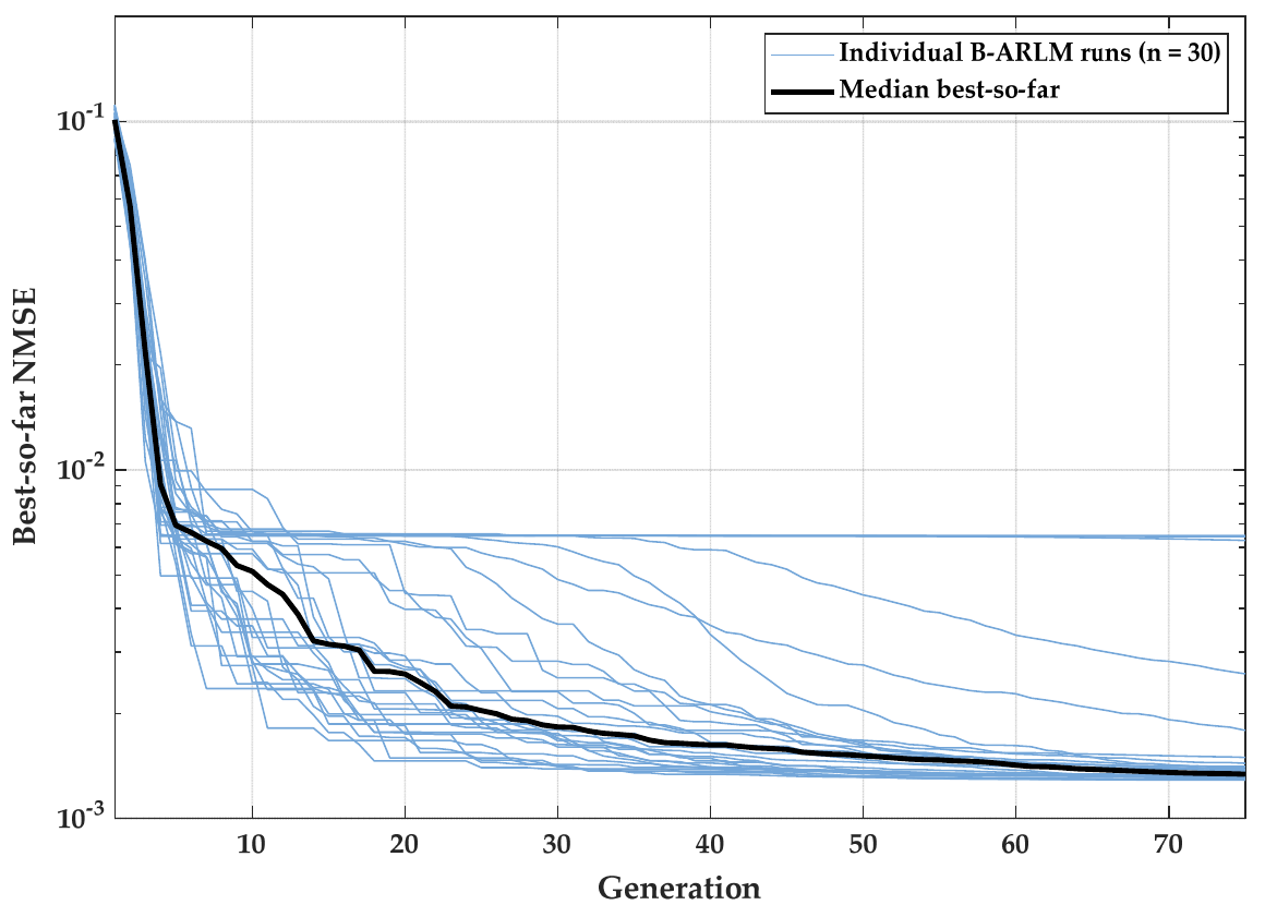
Figure 1 shows the best-so-far convergence histories of the 30 B-ARLM runs used in the reference-calibration experiment. The median curve summarizes the typical convergence behaviour across the independent runs.
7.3. Initial-Amplitude and Hyperparameter Sensitivity
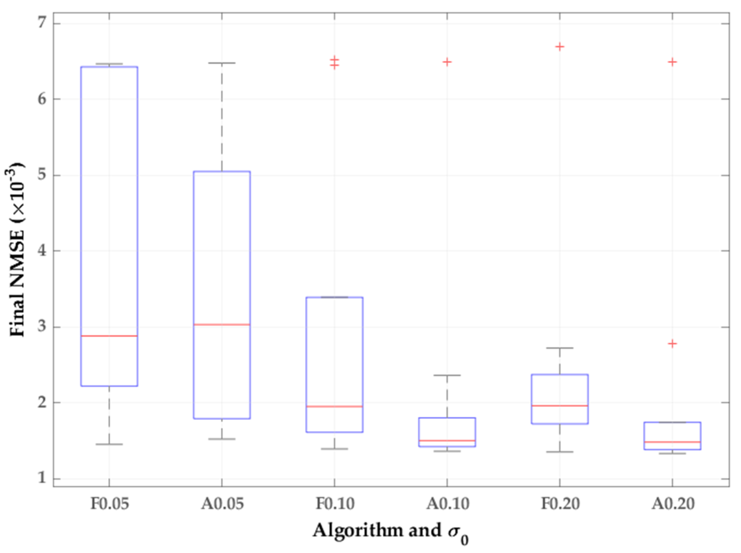
B-ARLM and Fixed-EA were compared using the three initial mutation amplitudes specified in Equation (13) (
Figure 2). For B-ARLM, σ
0 specifies only the initial parameter-wise mutation amplitude, whereas all three configurations use the same permanent upper bound, σ
max = 0.20. In contrast, Fixed-EA retains the selected mutation amplitude throughout each run. Each configuration was evaluated in 30 independent runs using a population size of 30, 75 generations, and the same bounds for all active parameters. For each value of σ
0, the corresponding B-ARLM and Fixed-EA runs used the same run-specific random seeds and identical initial populations.
Across the three tested initial amplitudes, B-ARLM showed less variation in central terminal performance than Fixed-EA, consistent with subsequent adaptation of the mutation amplitudes within the prescribed permanent bounds.
The broader one-factor-at-a-time sensitivity analysis comprised the reference configuration and 10 single-factor perturbations, with 30 paired runs per configuration. Across the examined finite ranges, median terminal NMSE values varied from approximately 1.30 × 10⁻³ to 1.47 × 10⁻³, compared with 1.36 × 10⁻³ for the reference setting. After Holm correction, only increasing the permanent lower mutation bound from σmin = 0.001 to 0.005 produced a statistically significant deterioration in terminal NMSE (pHolm ≈ 0.047).
The elevated lower bound also produced substantially greater lower-bound occupancy of the mutation amplitudes, consistent with insufficient late-stage contraction. None of the remaining tested hyperparameter perturbations remained statistically significant after multiplicity correction over the examined ranges. The reference setting is therefore retained as the predefined reference configuration, with limited sensitivity over the examined one-factor ranges, rather than interpreted as a globally optimized hyperparameter choice. Detailed sensitivity statistics and amplitude diagnostics are provided in the
Supplementary Materials.
7.4. Practical Identifiability, Global Parameter Compensation, and Observation Influence
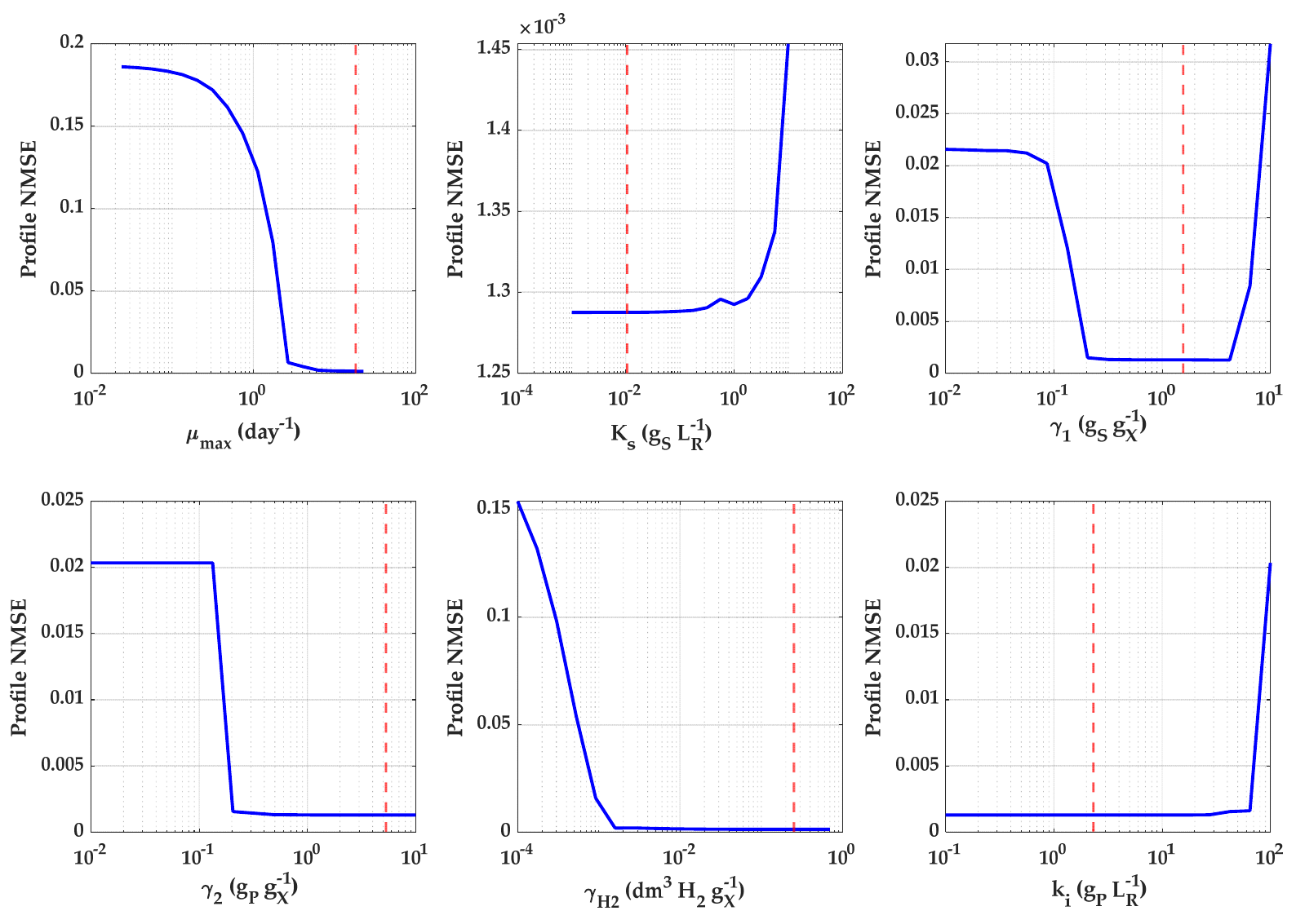
Practical parameter support was first examined through the profile-NMSE analysis shown in
Figure 3. The profiles characterize the extent to which each parameter can vary while the remaining parameters are re-optimized.
The profile-NMSE curves show markedly different levels of practical parameter support, including broad and asymmetric low-error regions consistent with parameter compensation. To test whether these features were specific to reference-centred initialization, 30 additional B-ARLM runs were initialized from Latin-hypercube populations spanning the full admissible domain. The best broad-start NMSE was 1.286 × 10⁻³, essentially identical to the reference value of 1.288 × 10⁻³; 16 of 30 runs remained within twice the best value. Despite these similar errors, the near-optimal vectors were widely separated, with a median normalized pairwise distance of 0.842 and a maximum of 1.534.
The strongest broad-start compensation involved
and
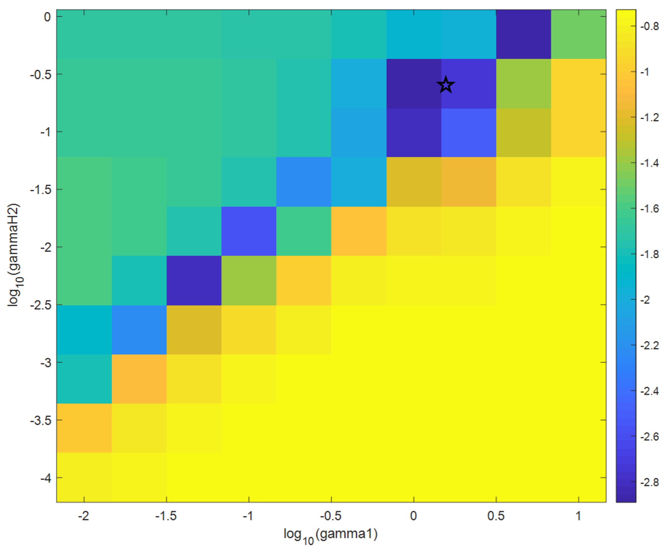
. Their two-dimensional profile produced a pronounced diagonal low-error valley; a distant combination near
= 4.22 and
= 0.70 retained an NMSE of approximately 1.30 × 10
−3, only about 0.8% above the reference optimum (see
Figure 4). Thus, the reference vector is not an isolated low-error parameter solution.
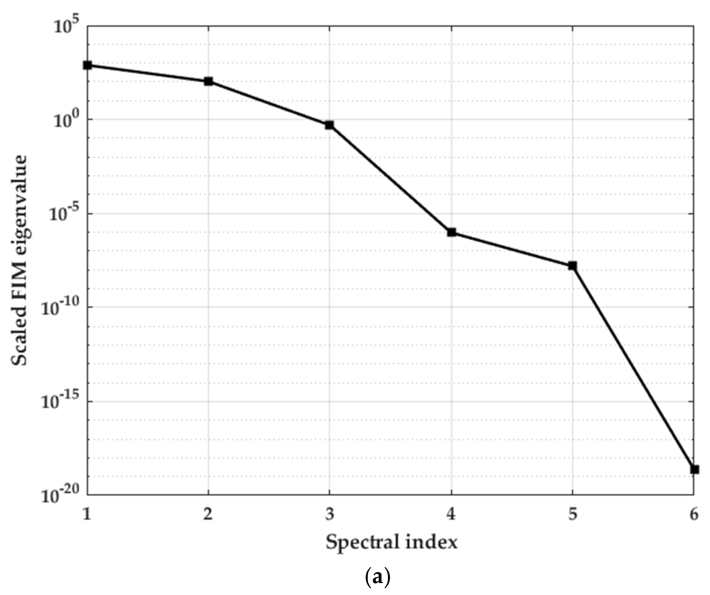
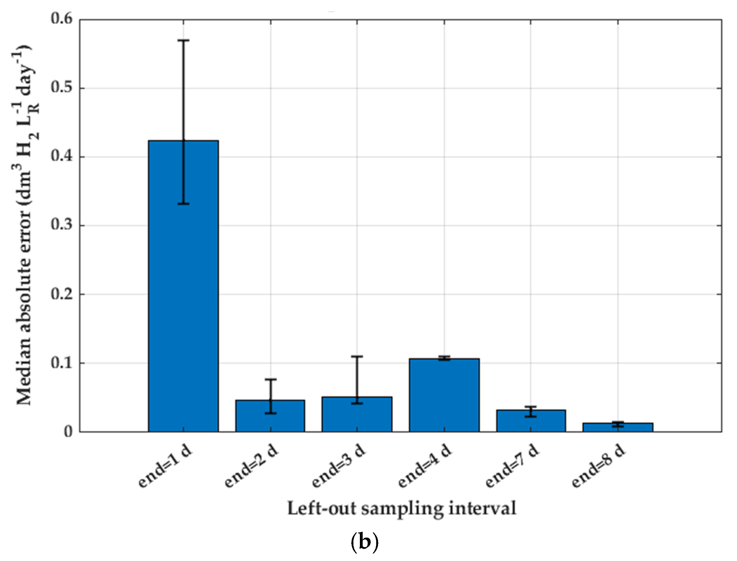
Local parameter support and observation influence were further examined using the scaled Fisher-information spectrum and repeated leave-one-out recalibration results shown in
Figure 5.
For the displayed reference vector, the scaled FIM eigenvalues span approximately 21.5 orders of magnitude, with a condition number of approximately 3.23 × 10²¹. The numerical rank was six, whereas the effective rank was five at all three examined relative singular-value thresholds; the smallest-scaled eigenvalue was approximately 2.40 × 10⁻¹⁹. These results indicate severe local ill-conditioning and weak support for at least one parameter combination.
The leave-one-interval-out analysis comprised 180 recalibrations. The 0–1 day interval was the most influential, followed by 3–4 days, whereas the late 4–7 and 7–8 day intervals produced the smallest median omitted-interval errors. Taken together, the profile, broad-start, two-dimensional, FIM, and leave-one-interval-out analyses show that accurate trajectory reconstruction is compatible with widely separated parameter vectors and uneven observation influence, indicating substantial practical non-identifiability without establishing structural non-identifiability.
7.5. Conditional Trajectory Uncertainty and Error-Model Sensitivity
Using the protocol defined in
Section 6.5, conditional fitted-trajectory uncertainty was evaluated at prescribed perturbation levels of 5% and 10%, with 200 synthetic datasets per level.
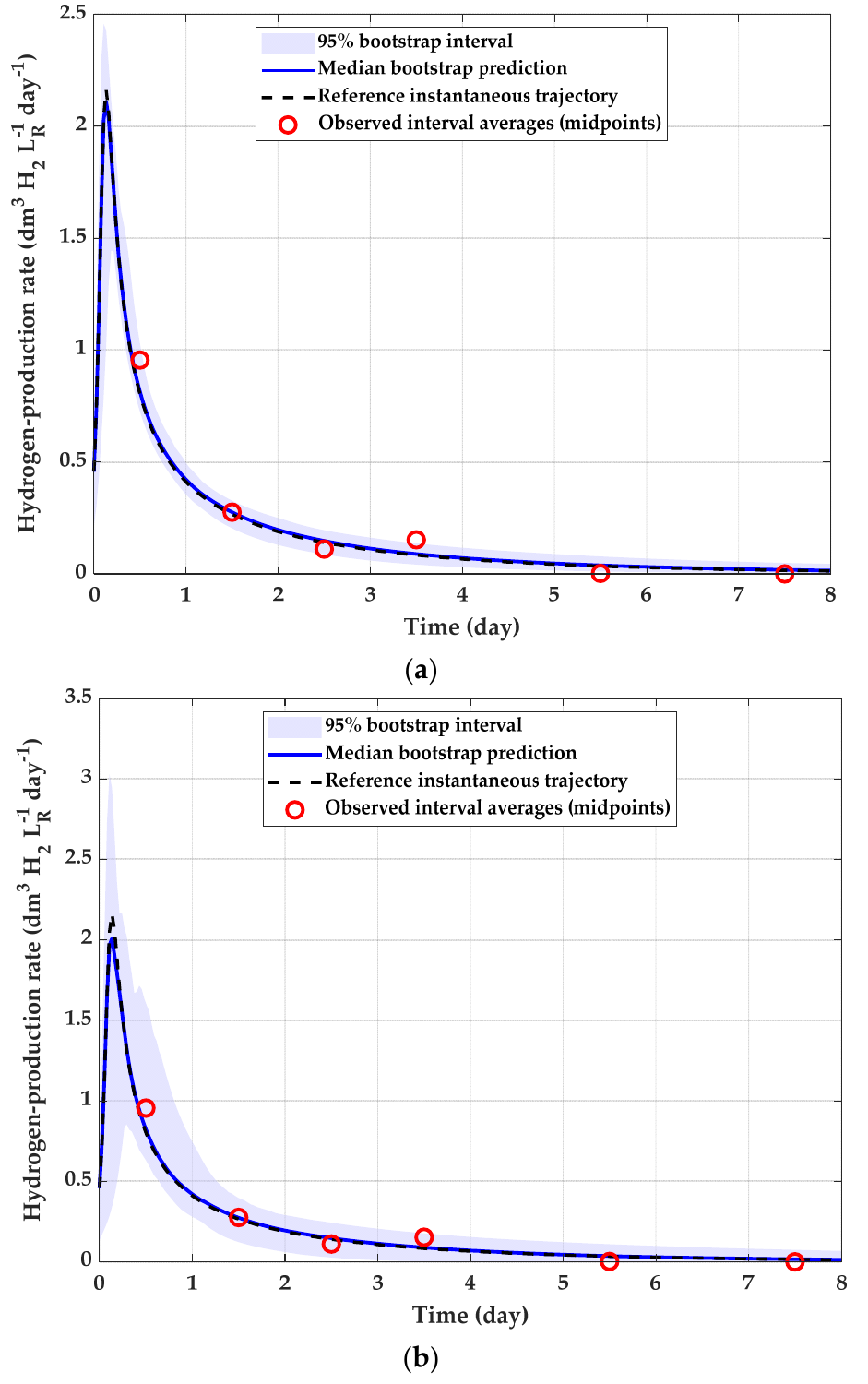
At both perturbation levels, the median trajectory retained the dominant early peak and subsequent decline. The conditional intervals were widest in the early dynamic region and narrowed during the late near-zero phase, indicating greater uncertainty in peak timing and magnitude than in the qualitative trajectory shape.
For the 5% perturbation level, the mean, median, and maximum pointwise 95% interval widths were 0.131, 0.0873, and 1.69
, respectively (see
Figure 6a). At the 10% perturbation level, the corresponding widths increased to 0.274, 0.154, and 2.74
(see
Figure 6b). The increases in all three width summaries at the 10% perturbation level are consistent with greater fitted-trajectory uncertainty under the larger imposed observation-perturbation scale.
The perturbation levels were not estimated from replicate-level measurement variance. Accordingly, the intervals characterize conditional fitted-trajectory uncertainty rather than replicate-derived confidence intervals or predictive intervals for future noisy observations. At the common 10% perturbation level, the mean pointwise 95% fitted-trajectory band width depended strongly on the assumed observation-error model: 0.280 for independent additive Gaussian noise, 0.101 for multiplicative log-normal noise, and 0.311 for additive Gaussian noise with first-order temporal correlation (AR(1), correlation coefficient = 0.5). Because replicate-level error statistics were unavailable, these results are interpreted as sensitivity to the prescribed error structure rather than evidence supporting any particular stochastic model.
7.6. Comparative Optimizer Performance
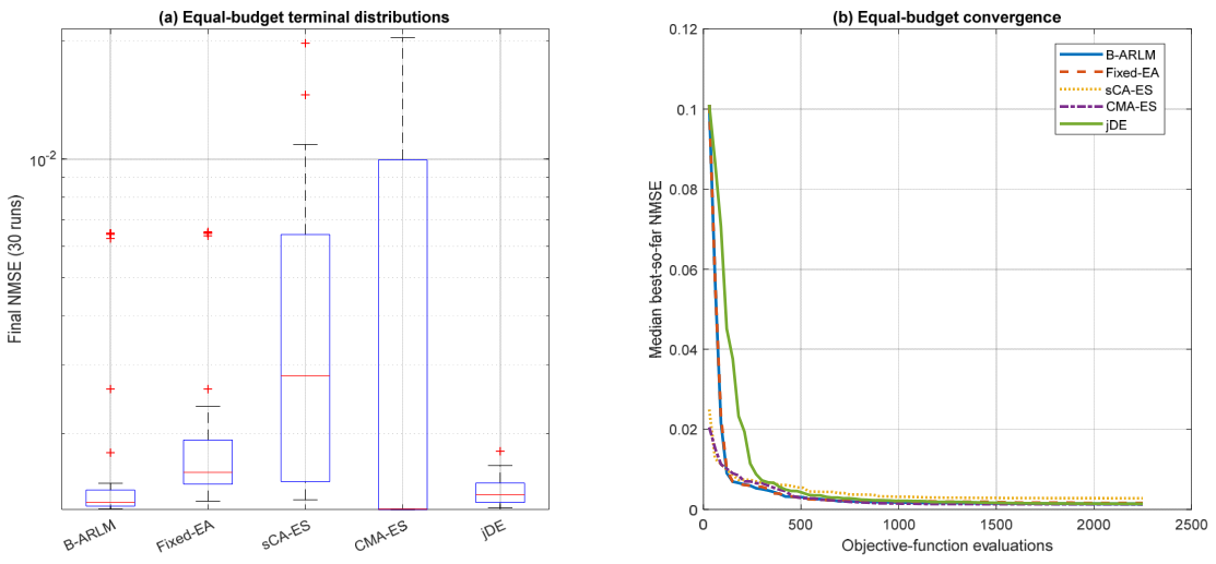
The matched-budget comparison of B-ARLM, Fixed-EA, sCA-ES, canonical CMA-ES, and jDE is summarized in
Table 4 and
Figure 7.
In contrast, terminal performance was not statistically distinguishable from canonical CMA-ES or jDE after Holm correction (pHolm ≈ 0.316 for both comparisons). CMA-ES achieved the lowest median NMSE but exhibited a pronounced upper tail, whereas jDE achieved the lowest mean, standard deviation, and worst-run NMSE among the five methods. B-ARLM therefore showed statistically supported improvement over its fixed-mutation ablation and the study-specific sCA-ES reference, while no statistically significant difference in terminal NMSE was detected between B-ARLM and CMA-ES or jDE under the present matched evaluation budget.
7.7. Computational Complexity and Runtime
With the production RK4 step, one objective evaluation required 9600 integration steps or 38,400 right-hand-side evaluations, corresponding to approximately 8.64 × 10
7 right-hand-side evaluations per 2250-evaluation run. B-ARLM requires
O(
Nd) working memory. Across five repeated measurements, the reference implementation required a median of 136.9 s per run (IQR 1.83 s). At the optimization layer, with
G generations, population size
N,
d active parameters, and
Cobj denoting the cost of one forward-model objective evaluation, the computational work scales as
O(
GN(
Cobj +
d)); for the present problem, this cost is dominated by RK4 forward integration. These timings characterize the present MATLAB implementation and are not interpreted as a runtime advantage over the comparator methods; additional details are provided in the
Supplementary Material.
8. Discussion
The present study considered sparse-data bioprocess calibration as a combined optimization and parameter-recovery problem. Among the three examined kinetic formulations, Andrews–P produced the lowest in-sample calibration error for the six interval-average observations. This result supports its use as the best-fitting formulation within the present dataset and calibration protocol, but it does not establish that the quadratic product-inhibition term is a uniquely correct biological mechanism or that Andrews–P has superior predictive performance outside the observed experiment.
The extended optimizer benchmark provides a more balanced assessment of B-ARLM than comparison with the study-specific references alone. Under the common budget of 2250 objective-function evaluations per run, B-ARLM significantly outperformed the Fixed-EA ablation and sCA-ES reference after Holm correction, whereas its terminal performance was not statistically distinguishable from canonical CMA-ES or jDE. CMA-ES achieved the lowest median terminal NMSE but exhibited a broad upper tail, while jDE produced the lowest mean, standard deviation, and worst-run NMSE. These results support B-ARLM as a competitive bounded calibration strategy for the present problem rather than as a universally superior optimizer.
This interpretation is consistent with the methodological position of B-ARLM relative to established evolutionary strategies. Success-based step-size adaptation, coordinate-dependent search scales, and covariance adaptation represent progressively richer mechanisms for modifying the search distribution [
28,
29,
30,
31,
32,
33,
34], while jDE adapts Differential Evolution control parameters through a different population-difference mechanism [
35]. B-ARLM does not reproduce the covariance learning of CMA-ES or the population-difference mutation of jDE; instead, it combines generation-level success control with bounded coordinate-wise scale learning. Its potential advantage is therefore not greater representational power, but a comparatively lightweight adaptation mechanism for bounded calibration problems.
The hyperparameter analysis further showed that performance was not dominated by most of the tested one-factor perturbations over the examined ranges. Only increasing the permanent lower mutation bound from 10−3 to 5 × 10⁻³ remained significantly detrimental after multiplicity correction, consistent with excessive lower-bound occupancy and reduced late-stage contraction. The reference settings should nevertheless be regarded as a predefined reference configuration showing limited sensitivity over the examined one-factor ranges, rather than as globally optimized hyperparameters. Similarly, the branch-wise contraction analysis establishes only local conditional behaviour: amplitude projection guarantees bounded internal mutation scales but does not provide a global stochastic-convergence theorem.
The identifiability results substantially qualify the interpretation of the low calibration errors. Local Fisher-information and one-dimensional profile analyses indicated severe ill-conditioning, while broad-start optimization and two-dimensional profiling showed that widely separated parameter vectors could retain nearly identical objective values. The pronounced (
and
) compensation valley demonstrates that this ambiguity is not restricted to the immediate neighbourhood of the reference solution. Such behaviour is consistent with the distinction between successful trajectory fitting and practical parameter identifiability emphasized in the identifiability literature [
12,
15,
18,
19,
42]. The leave-one-interval-out analysis further showed highly uneven observational influence, with the 0–1 day interval carrying substantially more information than the late near-zero intervals.
Fitted-trajectory uncertainty was also sensitive to the assumed observation-error structure. Additive Gaussian, multiplicative log-normal, and temporally correlated Gaussian perturbations produced materially different uncertainty band widths at the same nominal perturbation level. Because replicate-specific variance and temporal error statistics were unavailable, these scenarios should be interpreted as sensitivity analyses rather than identified experimental error laws. The principal limitations therefore remain the single sparse dataset, one measured output, six observations for six Andrews–P parameters, absence of independent predictive validation, lack of replicate-derived error statistics, and absence of formal structural-identifiability analysis. Broader assessment should include independent datasets, denser early-time sampling, additional measured states, and further dynamic model classes.
9. Conclusions
This proof-of-concept study evaluated B-ARLM as a bounded derivative-free strategy for parameter calibration in a sparse nonlinear bioprocess model. Among the three examined kinetic formulations, Andrews–P provided the lowest in-sample calibration error for the six interval-average observations. This result supports its use as the best-fitting formulation within the present dataset and calibration protocol but does not establish a uniquely correct biological inhibition mechanism or predictive superiority outside the observed experiment.
Under a common budget of 2250 objective-function evaluations per run, B-ARLM showed statistically significant improvement over the direct Fixed-EA ablation and the study-specific sCA-ES reference, while its terminal performance was not statistically distinguishable from canonical CMA-ES or jDE after Holm correction. The hyperparameter analysis indicated limited dependence on most examined one-factor perturbations, although an increased permanent lower mutation bound significantly degraded performance. These findings support B-ARLM as a competitive bounded calibration method for the present problem rather than as a universally superior optimizer.
The identifiability analyses showed that a low calibration error did not imply unique kinetic-parameter recovery. Broad-start optimization and two-dimensional profiling identified widely separated near-optimal parameter vectors and strong parameter compensation, while the fitted-trajectory uncertainty depended materially on the assumed observation-error structure. The main limitations remain the single sparse dataset, one measured output, absence of independent predictive validation, lack of replicate-derived error statistics, and absence of formal structural-identifiability analysis. Future work should evaluate B-ARLM on independent datasets, additional dynamic-model classes, and established benchmark problems. Further analysis is also required to characterize its convergence behaviour and computational performance beyond the present proof-of-concept setting.
Author Contributions
Conceptualization, V.L. and O.R.; methodology, V.L., O.R., and E.C.; software, V.L., O.R., A.Z., D.K., and G.R.; validation, V.L., O.R., E.C., and M.I.; formal analysis, V.L., O.R., E.C., and M.I.; investigation, V.L., O.R., E.C., A.Z., D.K., and G.R.; writing—original draft preparation, V.L., O.R., and E.C.; writing—review and editing, V.L., O.R., E.C., A.Z., D.K., and G.R.; visualization, D.K. and G.R. All authors have read and agreed to the published version of the manuscript.
Funding
This research received no external funding.
Institutional Review Board Statement
Not applicable.
Informed Consent Statement
Not applicable.
Data Availability Statement
The data supporting the findings of this study are contained within the article and
Supplementary Materials. Additional underlying experimental data are available from the corresponding author upon reasonable request.
Conflicts of Interest
The authors declare no conflicts of interest.
Abbreviations
| B-ARLM | Bounded Adaptive Random Local Mutation |
| CMA-ES | Covariance Matrix Adaptation Evolution Strategy |
| DE | Differential Evolution |
| FIM | Fisher Information Matrix |
| Fixed-EA | Fixed-Mutation Evolutionary Algorithm |
| IQR | Interquartile Range |
| jDE | Self-Adaptive Differential Evolution |
| LOO | Leave-One-Interval-Out |
| NMSE | Normalized Mean Squared Error |
| RK4 | Fourth-Order Runge–Kutta Method |
| sCA-ES | Simplified Covariance-Adaptive Evolution Strategy |
| Symbol | Definition |
| Calibrated parameter vector; the individual kinetic parameters and their units are defined in Table 2 |
| Admissible parameter domain |
| A | Set of active parameter-coordinate indices |
| Number of active calibrated parameters |
| Prescribed number of generations |
| Population size |
| Normalized least-squares calibration objective |
| Global best objective value available at generation |
| Set of candidates that improve upon the previous global best at generation |
| Generation-level success rate |
| Normalized mutation amplitude for parameter coordinate at generation |
| Initial mutation amplitude |
| Permanent lower and upper mutation-amplitude bounds |
| Target success rate |
| Coordinate-wise learning rate |
| Successful-displacement scale statistic for coordinate j |
| Multiplicative success-rate adaptation factor |
| Expansion/contraction factor |
| Instantaneous volumetric hydrogen-production rate |
| Log-parameter sensitivity matrix |
| Whitened log-parameter sensitivity matrix |
| Scaled Fisher-information matrix |
| Selected reference Andrews–P parameter vector |
| Minimum objective value attainable when parameter component is fixed at |
| Prescribed relative perturbation level |
| Prescribed sensitivity-whitening scale |
References
- Banga, J.R. Optimization in computational systems biology. BMC Syst. Biol. 2008, 2, 47. [Google Scholar] [CrossRef] [Scilit]
- Moles, C.G.; Mendes, P.; Banga, J.R. Parameter estimation in biochemical pathways: A comparison of global optimization methods. Genome Res. 2003, 13, 2467–2474. [Google Scholar] [CrossRef] [Scilit]
- Ashyraliyev, M.; Fomekong-Nanfack, Y.; Kaandorp, J.A.; Blom, J.G. Systems biology: Parameter estimation for biochemical models. FEBS J. 2009, 276, 886–902. [Google Scholar] [CrossRef] [Scilit]
- Grijspeerdt, K.; Vanrolleghem, P. Estimating the parameters of the Baranyi model for bacterial growth. Food Microbiol. 1999, 16, 593–605. [Google Scholar] [CrossRef] [Scilit]
- Akkermans, S.; Logist, F.; Van Impe, J.F. Parameter estimations in predictive microbiology: Statistically sound modelling of the microbial growth rate. Food Res. Int. 2018, 106, 1105–1113. [Google Scholar] [CrossRef] [Scilit]
- Zwietering, M.H.; Jongenburger, I.; Rombouts, F.M.; Van ’t Riet, K. Modeling of the bacterial growth curve. Appl. Environ. Microbiol. 1990, 56, 1875–1881. [Google Scholar] [CrossRef] [Scilit]
- Dochain, D. (Ed.) Bioprocess Control; Wiley-ISTE: London, UK, 2008. [Google Scholar] [CrossRef] [Scilit]
- Iglesias, P.A.; Ingalls, B.P. (Eds.) Control Theory and Systems Biology; MIT Press: Cambridge, MA, USA, 2010. [Google Scholar]
- Villadsen, J.; Nielsen, J.; Lidén, G. Bioreaction Engineering Principles, 3rd ed.; Springer: New York, NY, USA, 2011. [Google Scholar] [CrossRef] [Scilit]
- Joshi, H.; Jha, B.K. Modeling the spatiotemporal intracellular calcium dynamics in nerve cell with strong memory effects. Int. J. Nonlinear Sci. Numer. Simul. 2023, 24, 2383–2403. [Google Scholar] [CrossRef] [Scilit]
- Linden, N.J.; Kramer, B.; Rangamani, P. Bayesian parameter estimation for dynamical models in systems biology. PLoS Comput. Biol. 2022, 18, e1010651. [Google Scholar] [CrossRef] [Scilit]
- Simpson, M.J.; Maclaren, O.J. Profile-Wise Analysis: A profile likelihood-based workflow for identifiability analysis, estimation, and prediction with mechanistic mathematical models. PLoS Comput. Biol. 2023, 19, e1011515. [Google Scholar] [CrossRef] [Scilit]
- Murphy, R.J.; Maclaren, O.J.; Simpson, M.J. Implementing measurement error models with mechanistic mathematical models in a likelihood-based framework for estimation, identifiability analysis and prediction in the life sciences. J. R. Soc. Interface 2024, 21, 20230402. [Google Scholar] [CrossRef] [Scilit]
- Plank, M.J.; Simpson, M.J. Structured methods for parameter inference and uncertainty quantification for mechanistic models in the life sciences. R. Soc. Open Sci. 2024, 11, 240733. [Google Scholar] [CrossRef] [Scilit]
- Heinrich, M.; Rosenblatt, M.; Wieland, F.-G.; Stigter, H.; Timmer, J. On Structural and Practical Identifiability: Current Status and Update of Results. Curr. Opin. Syst. Biol. 2025, 41, 100546. [Google Scholar] [CrossRef] [Scilit]
- Heinrich, M.; Arutjunjan, R.; Timmer, J. On the Different Flavours of Practical Identifiability. Curr. Opin. Syst. Biol. 2025, 42, 100556. [Google Scholar] [CrossRef] [Scilit]
- Kreutz, C. An Easy and Efficient Approach for Testing Identifiability. Bioinformatics 2018, 34, 1913–1921. [Google Scholar] [CrossRef] [Scilit]
- Preston, S.P.; Wilkinson, R.D.; Clayton, R.H.; Chappell, M.J.; Mirams, G.R. Think before You Fit: Parameter Identifiability, Sensitivity and Uncertainty in Systems Biology Models. Curr. Opin. Syst. Biol. 2025, 42, 100563. [Google Scholar] [CrossRef] [Scilit]
- Wang, S.; Hao, W. A Systematic Computational Framework for Practical Identifiability Analysis in Mathematical Models Arising from Biology. Adv. Sci. 2025, 12, e04346. [Google Scholar] [CrossRef] [Scilit]
- Balsa-Canto, E.; Campo-Manzanares, N.; Moimenta, A.R.; Roudaut, G.; Troitiño-Jordedo, D. Quantifying and Managing Uncertainty in Systems Biology: Mechanistic and Data-Driven Models. Curr. Opin. Syst. Biol. 2025, 42, 100557. [Google Scholar] [CrossRef] [Scilit]
- Mendes, P.; Kell, D.B. Nonlinear optimization of biochemical pathways: Applications to metabolic engineering and parameter estimation. Bioinformatics 1998, 14, 869–883. [Google Scholar] [CrossRef] [Scilit]
- Balsa-Canto, E.; Banga, J.R. AMIGO, a toolbox for advanced model identification in systems biology using global optimization. Bioinformatics 2011, 27, 2311–2313. [Google Scholar] [CrossRef] [Scilit]
- Carlozo, M.N.; Wang, K.; Dowling, A.W. Bayesian optimization methods for nonlinear model calibration. Ind. Eng. Chem. Res. 2025, 64, 18277–18297. [Google Scholar] [CrossRef] [Scilit]
- Storn, R.; Price, K. Differential evolution—A simple and efficient heuristic for global optimization over continuous spaces. J. Glob. Optim. 1997, 11, 341–359. [Google Scholar] [CrossRef] [Scilit]
- Das, S.; Suganthan, P.N. Differential evolution: A survey of the state-of-the-art. IEEE Trans. Evol. Comput. 2011, 15, 4–31. [Google Scholar] [CrossRef] [Scilit]
- Price, K.V.; Storn, R.M.; Lampinen, J.A. Differential Evolution: A Practical Approach to Global Optimization; Springer: Berlin/Heidelberg, Germany, 2005. [Google Scholar] [CrossRef] [Scilit]
- Kennedy, J.; Eberhart, R.C. Particle swarm optimization. In Proceedings of the IEEE International Conference on Neural Networks (ICNN’95), Perth, Australia, 27 November–1 December 1995; pp. 1942–1948. [Google Scholar] [CrossRef] [Scilit]
- Hansen, N.; Ostermeier, A. Completely derandomized self-adaptation in evolution strategies. Evol. Comput. 2001, 9, 159–195. [Google Scholar] [CrossRef] [Scilit]
- Bäck, T. Evolutionary Algorithms in Theory and Practice: Evolution Strategies, Evolutionary Programming, Genetic Algorithms; Oxford University Press: New York, NY, USA, 1996. [Google Scholar]
- Beyer, H.-G.; Schwefel, H.-P. Evolution strategies—A comprehensive introduction. Nat. Comput. 2002, 1, 3–52. [Google Scholar] [CrossRef] [Scilit]
- Morinaga, D.; Fukuchi, K.; Sakuma, J.; Akimoto, Y. Convergence Rate of the (1+1)-Evolution Strategy with Success-Based Step-Size Adaptation on Convex Quadratic Functions. In Proceedings of the Genetic and Evolutionary Computation Conference (GECCO ’21), Lille, France, 10–14 July 2021; pp. 1169–1177. [Google Scholar] [CrossRef] [Scilit]
- Akimoto, Y.; Auger, A.; Glasmachers, T.; Morinaga, D. Global Linear Convergence of Evolution Strategies on More Than Smooth Strongly Convex Functions. SIAM J. Optim. 2022, 32, 1402–1429. [Google Scholar] [CrossRef] [Scilit]
- Hansen, N. The CMA Evolution Strategy: A Tutorial. arXiv 2016, arXiv:1604.00772. [Google Scholar] [CrossRef] [Scilit]
- Akimoto, Y.; Hansen, N. Diagonal Acceleration for Covariance Matrix Adaptation Evolution Strategies. Evol. Comput. 2020, 28, 405–435. [Google Scholar] [CrossRef] [Scilit]
- Brest, J.; Greiner, S.; Bošković, B.; Mernik, M.; Žumer, V. Self-Adapting Control Parameters in Differential Evolution: A Comparative Study on Numerical Benchmark Problems. IEEE Trans. Evol. Comput. 2006, 10, 646–657. [Google Scholar] [CrossRef] [Scilit]
- Sun, W.; Yuan, Y.-X. Optimization Theory and Methods: Nonlinear Programming; Springer: New York, NY, USA, 2006. [Google Scholar] [CrossRef] [Scilit]
- Edgar, T.F.; Himmelblau, D.M.; Lasdon, L.S. Optimization of Chemical Processes, 2nd ed.; McGraw-Hill: New York, NY, USA, 2001. [Google Scholar]
- Schittkowski, K. Numerical Data Fitting in Dynamical Systems: A Practical Introduction with Applications and Software; Kluwer Academic Publishers: Dordrecht, The Netherlands, 2002. [Google Scholar]
- Bäck, T.H.W.; Kononova, A.V.; van Stein, B.; Wang, H.; Antonov, K.A.; Kalkreuth, R.T.; de Nobel, J.; Vermetten, D.; de Winter, R.; Ye, F. Evolutionary Algorithms for Parameter Optimization—Thirty Years Later. Evol. Comput. 2023, 31, 81–122. [Google Scholar] [CrossRef] [Scilit]
- Eiben, A.E.; Jelasity, M. A Critical Note on Experimental Research Methodology in EC. In Proceedings of the 2002 Congress on Evolutionary Computation (CEC 2002), Honolulu, HI, USA, 12–17 May 2002; Volume 1, pp. 582–587. [Google Scholar] [CrossRef] [Scilit]
- Birattari, M.; Dorigo, M. How to Assess and Report the Performance of a Stochastic Algorithm on a Benchmark Problem: Mean or Best Result on a Number of Runs? Optim. Lett. 2007, 1, 309–311. [Google Scholar] [CrossRef] [Scilit]
- Raue, A.; Kreutz, C.; Maiwald, T.; Bachmann, J.; Schilling, M.; Klingmüller, U.; Timmer, J. Structural and Practical Identifiability Analysis of Partially Observed Dynamical Models by Exploiting the Profile Likelihood. Bioinformatics 2009, 25, 1923–1929. [Google Scholar] [CrossRef] [Scilit]
- Chis, O.-T.; Banga, J.R.; Balsa-Canto, E. Structural Identifiability of Systems Biology Models: A Critical Comparison of Methods. PLoS ONE 2011, 6, e27755. [Google Scholar] [CrossRef] [Scilit]
- Efron, B.; Tibshirani, R.J. An Introduction to the Bootstrap; Chapman & Hall: New York, NY, USA, 1993. [Google Scholar]
- Monod, J. The Growth of Bacterial Cultures. Annu. Rev. Microbiol. 1949, 3, 371–394. [Google Scholar] [CrossRef] [Scilit]
- Andrews, J.F. A Mathematical Model for the Continuous Culture of Microorganisms Utilizing Inhibitory Substrates. Biotechnol. Bioeng. 1968, 10, 707–723. [Google Scholar] [CrossRef] [Scilit]
- Van den Heuvel, J.C.; Beeftink, H.H. Kinetic Effects of Simultaneous Inhibition by Substrate and Product. Biotechnol. Bioeng. 1988, 31, 718–724. [Google Scholar] [CrossRef] [Scilit]
Figure 1.
Best-so-far NMSE convergence trajectories of B-ARLM for the Andrews–P model over 30 independent runs. Thin blue curves represent individual optimization runs, while the thick black curve denotes the pointwise median best-so-far NMSE. Each run used a population of 30 individuals for 75 generations. The NMSE axis is logarithmic.
Figure 1.
Best-so-far NMSE convergence trajectories of B-ARLM for the Andrews–P model over 30 independent runs. Thin blue curves represent individual optimization runs, while the thick black curve denotes the pointwise median best-so-far NMSE. Each run used a population of 30 individuals for 75 generations. The NMSE axis is logarithmic.
Figure 2.
Terminal NMSE distributions over 30 runs for Fixed-EA (F) and B-ARLM (A) at the three tested mutation-amplitude settings σ0 = 0.05, 0.10, and 0.20. For B-ARLM, σ0 denotes the initial mutation amplitude, whereas Fixed-EA retains the selected amplitude throughout the run. Corresponding B-ARLM and Fixed-EA runs used matched random seeds and identical initial populations.
Figure 2.
Terminal NMSE distributions over 30 runs for Fixed-EA (F) and B-ARLM (A) at the three tested mutation-amplitude settings σ0 = 0.05, 0.10, and 0.20. For B-ARLM, σ0 denotes the initial mutation amplitude, whereas Fixed-EA retains the selected amplitude throughout the run. Corresponding B-ARLM and Fixed-EA runs used matched random seeds and identical initial populations.
Figure 3.
Profile-NMSE curves for the six calibrated Andrews–P parameters. Dashed vertical lines indicate the reference parameter values. For each parameter, 17 logarithmically spaced base-grid values were augmented with the reference value. At each grid point, the remaining parameters were re-optimized in three independent B-ARLM runs using 50 generations and a population size of 20, and the lowest obtained NMSE was retained as the profile value.
Figure 3.
Profile-NMSE curves for the six calibrated Andrews–P parameters. Dashed vertical lines indicate the reference parameter values. For each parameter, 17 logarithmically spaced base-grid values were augmented with the reference value. At each grid point, the remaining parameters were re-optimized in three independent B-ARLM runs using 50 generations and a population size of 20, and the lowest obtained NMSE was retained as the profile value.
Figure 4.
Two-dimensional profile-NMSE map for and . At each grid point, the two displayed parameters were fixed, and the remaining four Andrews–P parameters were re-optimized in two B-ARLM runs using a population size of 20 and 40 generations. The star (★) denotes the reference parameter combination associated with the best-fit solution. The color scale represents log10 of the profile NMSE; the diagonal low-error region indicates strong parameter compensation.
Figure 4.
Two-dimensional profile-NMSE map for and . At each grid point, the two displayed parameters were fixed, and the remaining four Andrews–P parameters were re-optimized in two B-ARLM runs using a population size of 20 and 40 generations. The star (★) denotes the reference parameter combination associated with the best-fit solution. The color scale represents log10 of the profile NMSE; the diagonal low-error region indicates strong parameter compensation.
Figure 5.
Practical-identifiability and interval-influence diagnostics. (a) local-scaled Fisher-information eigenvalue spectrum based on whitened log-parameter sensitivities. (b) median absolute leave-one-interval-out prediction errors over 30 independent recalibrations per omitted interval, with error bars denoting the interquartile range.
Figure 5.
Practical-identifiability and interval-influence diagnostics. (a) local-scaled Fisher-information eigenvalue spectrum based on whitened log-parameter sensitivities. (b) median absolute leave-one-interval-out prediction errors over 30 independent recalibrations per omitted interval, with error bars denoting the interquartile range.
Figure 6.
Conditional parametric-bootstrap fitted-trajectory uncertainty. Shaded regions denote pointwise 95% empirical trajectory intervals; solid and dashed curves represent the median recalibrated and reference Andrews–P instantaneous trajectories, respectively; circles denote the observed interval-average rates plotted at the interval midpoints. (a) 5% prescribed additive Gaussian perturbations with clipping at zero. (b) 10% prescribed additive Gaussian perturbations with clipping at zero.
Figure 6.
Conditional parametric-bootstrap fitted-trajectory uncertainty. Shaded regions denote pointwise 95% empirical trajectory intervals; solid and dashed curves represent the median recalibrated and reference Andrews–P instantaneous trajectories, respectively; circles denote the observed interval-average rates plotted at the interval midpoints. (a) 5% prescribed additive Gaussian perturbations with clipping at zero. (b) 10% prescribed additive Gaussian perturbations with clipping at zero.
Figure 7.
Comparative optimizer performance over 30 runs per method under a common budget of 2250 objective-function evaluations per run: (a) terminal NMSE distributions; (b) median best-so-far NMSE as a function of objective-function evaluations.
Figure 7.
Comparative optimizer performance over 30 runs per method under a common budget of 2250 objective-function evaluations per run: (a) terminal NMSE distributions; (b) median best-so-far NMSE as a function of objective-function evaluations.
Table 1.
Conceptual positioning of B-ARLM relative to representative mutation-scale adaptation mechanisms.
Table 1.
Conceptual positioning of B-ARLM relative to representative mutation-scale adaptation mechanisms.
| Method Family | Scale Representation | Primary Adaptation Signal | Cross-Parameter Covariance | Relation to B-ARLM |
|---|
Fixed
mutation | Fixed scalar or parameter-wise amplitudes | None | No | Control variant in which the adaptive
amplitude updates are disabled |
Scalar
success-based ES | One adaptive global step size | Success rate or success history | No | Related to the
generation-level
multiplicative update |
| Coordinate-dependent/diagonal adaptation (e.g., diagonal/sep-CMA-ES) | Separate coordinate-wise scales or diagonal covariance representation | Diagonal statistics or strategy-parameter
updates | Usually
absent or
restricted | Related to parameter-wise scale learning |
Full
covariance adaptation | Global scale and covariance matrix | Ranked samples,
evolution paths, and
covariance updates | Yes | Represents correlations that B-ARLM does not estimate |
| B-ARLM | Bounded
parameter-wise amplitudes | Generation-level success rate and median absolute coordinate-wise
displacements of
successful candidates | No | Combines bounded
coordinate-wise
amplitudes with
success-rate and
successful-displacement updates |
| Adaptive Differential Evolution | Mutation factor and crossover parameters | Population differences and adaptive control parameters | No explicit covariance matrix | Different population-difference mechanism; represented experimentally by jDE |
Table 2.
Model parameters, definitions, units, nominal values, and calibration bounds.
Table 2.
Model parameters, definitions, units, nominal values, and calibration bounds.
| Symbol | Definition | Unit | Nominal | Lower | Upper |
|---|
| Maximum specific growth rate | day−1 | 4.8 | 0.024 | 22.8 |
| Substrate half-saturation constant | gL−1 | 0.05 | 0.001 | 10 |
| Substrate-consumption coefficient | −1 | 5.0 | 0.01 | 10 |
| Product-formation coefficient | −1 | 5.0 | 0.01 | 10 |
| Hydrogen-production yield coefficient | −1 | 0.0694 | 0.0001 | 0.7 |
| Product-inhibition scale in | gL−1 | 50.0 | 0.1 | 100 |
Table 3.
Comparative in-sample calibration performance of the tested kinetic formulations over 30 independent B-ARLM runs.
Table 3.
Comparative in-sample calibration performance of the tested kinetic formulations over 30 independent B-ARLM runs.
| Model | k | Best
NMSE | Worst
NMSE | Mean NMSE | SD
NMSE |
|---|
| Monod | 5 | 6.48 × 10⁻³ | 2.03 × 10⁻² | 9.71 × 10⁻³ | 5.96 × 10⁻³ |
| Andrews–G | 6 | 6.48 × 10⁻³ | 2.03 × 10⁻² | 8.79 × 10⁻³ | 5.25 × 10⁻³ |
| Andrews–P | 6 | 1.29 × 10⁻³ | 6.47 × 10⁻³ | 2.08 × 10⁻³ | 1.75 × 10⁻³ |
Table 4.
Terminal optimizer performance over 30 runs per method under a common budget of 2250 objective-function evaluations per run. IQR denotes the interquartile range. Formal pairwise comparisons of B-ARLM with the four reference methods were Holm-adjusted as described in
Section 5.5.
Table 4.
Terminal optimizer performance over 30 runs per method under a common budget of 2250 objective-function evaluations per run. IQR denotes the interquartile range. Formal pairwise comparisons of B-ARLM with the four reference methods were Holm-adjusted as described in
Section 5.5.
| Optimizer | Median NMSE | IQR | Mean NMSE | SD | Worst NMSE |
|---|
| B-ARLM | 1.339 × 10⁻³ | 1.21 × 10⁻⁴ | 2.076 × 10⁻³ | 1.748 × 10⁻³ | 6.473 × 10⁻³ |
| Fixed-EA | 1.597 × 10⁻³ | 4.14 × 10⁻⁴ | 2.299 × 10⁻³ | 1.687 × 10⁻³ | 6.531 × 10⁻³ |
| sCA-ES | 2.806 × 10⁻³ | 4.90 × 10⁻³ | 4.929 × 10⁻³ | 4.513 × 10⁻³ | 1.972 × 10⁻² |
| CMA-ES | 1.286 × 10⁻³ | 8.41 × 10⁻³ | 5.781 × 10⁻³ | 6.815 × 10⁻³ | 2.034 × 10⁻² |
| jDE | 1.401 × 10⁻³ | 1.55 × 10⁻⁴ | 1.439 × 10⁻³ | 1.28 × 10⁻⁴ | 1.806 × 10⁻³ |
| Disclaimer/Publisher’s Note: The statements, opinions and data contained in all publications are solely those of the individual author(s) and contributor(s) and not of MDPI and/or the editor(s). MDPI and/or the editor(s) disclaim responsibility for any injury to people or property resulting from any ideas, methods, instructions or products referred to in the content. |




 ,
,