Well-Posedness of Flux–Fractional Compartment Models and Their State Sensitivity Systems

Abstract

We studied flux–fractional compartment models with Caputo memory terms and their associated state sensitivity systems. The state, classical parameter sensitivities, and fractional-order sensitivity are formulated within a unified linear Volterra framework. Using a Sobolev-space formulation and an equivalent Bielecki norm, we establish existence and uniqueness in $W^{1,p}(0,T;H)$ on arbitrary finite time intervals. We further prove continuous differentiability of the parameter-to-solution map and derive a dimensionally consistent fractional-order sensitivity involving a dimensionless logarithmic kernel. The theory is illustrated by a one-compartment model with explicit Mittag–Leffler representations and relative sensitivity analysis.

1. Introduction and Motivation

Classical pharmacokinetic models are commonly formulated as systems of first-order ordinary differential equations and therefore generate exponential-type transfer and elimination profiles. However, experimental and clinical data may exhibit systematic deviations from purely exponential behavior, including long-time tails and history-dependent transport. Such effects are naturally associated with memory and anomalous transport and are well documented in the theory of continuous-time random walks and anomalous diffusion [1].

Fractional derivatives provide a natural mechanism for incorporating nonlocal temporal effects into pharmacokinetic and biological transport models. They have been used to describe anomalous diffusion, tissue trapping, and non-exponential transport phenomena that are not adequately captured by classical compartment equations [2,3,4]. In the present work, the fractional operator is attached to the compartmental flux rather than used to replace the entire state derivative.

Recent studies have developed fractional compartment models from phenomenological and stochastic-process viewpoints, with particular attention to dimensional consistency, mass balance, numerical approximation, parameter estimation, and sensitivity analysis [5,6,7,8,9,10,11]. Fractional-order sensitivities have also been investigated numerically through finite parameter perturbations [10]. The present work differs by proving continuous differentiability of the parameter-to-solution map in $W^{1,p}$ with respect to both the classical parameters and the fractional order, and by deriving the corresponding sensitivity equations analytically.

We consider the forced flux–fractional compartment system

$$\dot{q}\left(t\right)=A(\theta ,\alpha )q\left(t\right)+B(\theta ,\alpha ){}^{\mathrm{C}}D_{0+}^{1-\alpha }q\left(t\right)+b(t,\theta ,\alpha ),$$

together with its sensitivities with respect to the classical parameter vector $\theta$ and the fractional order $\alpha$. The placement of the fractional operator on the flux is consistent with compartmental fractionalization procedures designed to preserve the physical meaning of transfer processes, dimensional consistency, and mass balance [5,6,7].

As a scalar specialization, we consider the one-compartment model [4,5]

$$A^{\prime }\left(t\right)=k_{01}-k_{10,f}{}^{\mathrm{C}}D_{0+}^{1-\alpha }A\left(t\right).$$

A central mathematical issue is the differentiation of the solution with respect to the fractional order. Differentiation with respect to a classical parameter modifies the coefficients, forcing term, and initial data while leaving the fractional operator fixed. By contrast, variation in $\alpha$ affects both the solution and the kernel defining the fractional operator. Thus,

$${\partial }_{\alpha }\left({}^{\mathrm{C}}D_{0+}^{1-\alpha }q\right)={}^{\mathrm{C}}D_{0+}^{1-\alpha }{S}_{\alpha }+\left({\partial }_{\alpha }^{\mathrm{op}}{}^{\mathrm{C}}D_{0+}^{1-\alpha }\right)q,S_{\alpha }={\partial }_{\alpha }q,$$

where the operator derivative is taken with the state held fixed. This decomposition produces a logarithmically weighted memory kernel that is absent from the classical parameter sensitivities.

To retain dimensional consistency in the order derivative, we introduce a fixed reference time $t_{*}>0$. In the one-compartment model, the dimensionless quantity $\kappa =k_{10,f}{t}_{*}^{\alpha }$ is held fixed as $\alpha$ varies. The resulting logarithmic contribution is expressed through $ln\left((t-\tau )/t_{*}\right)$, leading to the logarithmically weighted Caputo operator ${}^{\mathrm{C}}D_{0+}^{1-\alpha ,ln,t_{*}}$. This reference-time normalization is essential because a direct differentiation with respect to $\alpha$ would otherwise introduce the logarithm of a dimensional quantity.

The analysis is carried out in the Sobolev space $W^{1,p}(0,T;H)$, $1<p<\infty$. In this space, both the Caputo operator and the logarithmically weighted order-derivative operator act continuously into $L^p(0,T;H)$. Consequently, the state, the classical sensitivities, and the fractional-order sensitivity can be studied within a common Sobolev–Volterra framework.

The well-posedness theory for linear Volterra equations with integrable and weakly singular kernels is classical. Here, the augmented state–sensitivity system is reduced to a Volterra equation for the velocity and analyzed in an exponentially weighted $L^p$ norm. The Bielecki-weighted contraction argument yields existence and uniqueness on arbitrary finite time intervals. The contribution is therefore not a new fixed-point principle, but its application to the coupled flux–fractional state–sensitivity system, including the logarithmically weighted fractional-order term.

More precisely, the main contributions are the formulation of a forced flux–fractional compartment system including the derivatives of the forcing term and initial data, the simultaneous derivation of the classical and fractional-order sensitivity equations, the construction of a dimensionally consistent logarithmic order derivative, and the proof that

$$(\theta ,\alpha )⟼q(·;\theta ,\alpha )$$

is continuously differentiable as a map into $W^{1,p}(0,T;{\mathbb{R}}^m)$. Hence, the sensitivity variables are genuine derivatives of the solution map rather than quantities introduced only by formal differentiation.

The one-compartment flux–fractional model is then used to illustrate the theory. Its triangular state–sensitivity structure yields Mittag–Leffler and Volterra-resolvent representations and permits a direct comparison of the corresponding relative sensitivities.

The paper is organized as follows. Section 2 introduces the fractional operators and the Sobolev-space preliminaries. Section 3 formulates the forced flux–fractional compartment model and derives the classical and fractional-order sensitivity equations. Section 4 establishes well-posedness on arbitrary finite time intervals and proves continuous differentiability of the parameter-to-solution map. Section 5 examines the one-compartment model and its relative sensitivities.

2. Fractional Calculus

Fractional calculus provides a natural mathematical framework to describe processes with memory and hereditary effects, which arise frequently in physics, biology, and pharmacokinetics [2,3,4]. In contrast to classical differential equations, fractional-order models account for the cumulative influence of the past evolution of the system, leading to nonlocal-in-time operators [1,3].

Since several inequivalent notions of fractional differentiation coexist in the literature, it is essential to clearly state the definitions and conventions used throughout this work [3,12]. We therefore briefly recall the Riemann–Liouville and Caputo fractional derivatives, emphasize their structural differences, and clarify their respective roles in modeling and analysis. This overview also serves to fix notation and to motivate the choice of the Caputo derivative in the pharmacokinetic models studied later [4,10].

Riemann–Liouville (RL) fractional derivative: As a first notion of fractional differentiation, we recall the Riemann–Liouville (RL) derivative. Derivatives of integer order $n\in \mathbb{N}$ for functions $f:\mathbb{R}\to \mathbb{R}$ belong to the classical theory of analysis. To extend differentiation to noninteger orders $\alpha \in \mathbb{R}$, we begin with the Riemann–Liouville (RL) fractional integral, constructed from Cauchy’s iterated integrals:

$$\left(I_{0+}^{\alpha }f\right)\left(t\right):={\displaystyle \frac{1}{\Gamma \left(\alpha \right)}}{\int }_0^t{(t-\xi )}^{\alpha -1}f\left(\xi \right)d\xi ,\alpha >0.$$

(1)

Here $\Gamma$ denotes Euler’s gamma function. We fix a finite time horizon $T>0$ and consider all fractional operators on the interval $(0,T)$. Operator (1) is well defined, for example, for $f\in L_{\mathrm{loc}}^1(0,T)$; for $\alpha \in \mathbb{N}$ it reduces to the usual $\alpha$–fold integral. Throughout this work we mainly consider orders $0<\alpha <1$. The subscript 0 indicates the lower limit of the operator: in $I_{0+}^{\alpha }$ the integral runs from 0 up to the current time t. Consequently, only the values of $f\left(\xi \right)$ with $0\le \xi \le t$ enter the integral, while data prior to time 0 are ignored. This corresponds to assuming that the system starts evolving at $t=0$. More generally one writes $I_{a+}^{\alpha }$ with any $a\in \mathbb{R}$. Choosing $a=-\infty$ yields Weyl-type fractional operators, whose convolution integrals extend over the entire past $(-\infty ,t)$ and which are invariant under time translations. Such operators are appropriate when the underlying process is assumed to possess an infinitely long prehistory [2].

A left-sided RL fractional derivative is obtained by differentiating an integral of complementary order. For $0<\alpha <1$ we define

$$\left(D_{0+}^{\alpha }f\right)\left(t\right):={\displaystyle \frac{d}{dt}}\left(I_{0+}^{1-\alpha }f\right)\left(t\right)={\displaystyle \frac{1}{\Gamma (1-\alpha )}}{\displaystyle \frac{d}{dt}}{\int }_0^t{(t-\xi )}^{-\alpha }f\left(\xi \right)d\xi .$$

(2)

The first equality in Equation (2) is the definition of the Riemann–Liouville fractional derivative, while the second equality follows from inserting the explicit representation of the fractional integral. The operator $D_{0+}^{\alpha }f$ is well defined whenever $I_{0+}^{1-\alpha }f$ is absolutely continuous on $(0,T)$, for instance when $I_{0+}^{1-\alpha }f\in W^{1,1}(0,T)$. Throughout, the symbol ∗ denotes convolution in time, defined for locally integrable functions by

$$(g\ast f)\left(t\right):={\int }_0^{t}g(t-\tau )f\left(\tau \right)d\tau ,t\in (0,T).$$

We work with functions in $L_{\mathrm{loc}}^1(0,T)$, so all integrals are understood on compact subintervals of $(0,T)$. Moreover, $\mathcal{L}\left\{f\right\}\left(s\right)=\widehat{f}\left(s\right)$ denotes the Laplace transform, following the conventions in [13,14].

For $\alpha >0$, define the power law kernel

$$g_{\alpha }\left(t\right):={\displaystyle \frac{t^{\alpha -1}}{\Gamma \left(\alpha \right)}},t>0.$$

(3)

With this notation, the Riemann–Liouville fractional integral can be written compactly as

$$I_{0+}^{\alpha }f=g_{\alpha }\ast f.$$

Although integral Formula (1) is stated for $\alpha >0$, the family of Riemann–Liouville fractional integrals ${\left\{I_{0+}^{\alpha }\right\}}_{\alpha >0}$ admits a continuous extension to $\alpha =0$ on $(0,T)$ in $L^p$ sense, for every $1\le p<\infty$. This is made precise in the next lemma, where we show that $I_{0+}^{\alpha }f\to f$ in $L^p(0,T)$ as $\alpha \to 0^{+}$ for all $f\in L^p(0,T)$, and hence it is natural to set $I_{0+}^{0}f:=f$.

Lemma 1

($L^p$–continuity at $\alpha =0$). Let $1\le p<\infty$ and $T>0$. Then, for every $\alpha >0$, the Riemann–Liouville fractional integral $I_{0+}^{\alpha }$ maps $L^p(0,T)$ into itself and satisfies

$$\parallel I_{0+}^{\alpha }{f\parallel }_{L^p(0,T)}\le \left({\int }_0^T{g}_{\alpha }\left(\tau \right)d\tau \right){\parallel f\parallel }_{L^p(0,T)}={\displaystyle \frac{T^{\alpha }}{\Gamma (\alpha +1)}}{\parallel f\parallel }_{L^p(0,T)}.$$

Moreover,

$$\underset{\alpha \to 0^{+}}{lim}{\parallel I_{0+}^{\alpha }f-f\parallel }_{L^p(0,T)}=0\mathrm{for}\mathrm{all}f\in L^p(0,T).$$

In particular, defining $I_{0+}^0:=\mathrm{Id}$ yields a continuous extension of $\alpha \mapsto I_{0+}^{\alpha }$ at $\alpha =0$ in $L^p(0,T)$.

Proof. 

Let

$$g_{\alpha }\left(t\right)={\displaystyle \frac{t^{\alpha -1}}{\Gamma \left(\alpha \right)}},t>0,$$

and set

$$k_{\alpha }:=g_{\alpha }{\mathbf{1}}_{(0,T)}\in L^1\left(\mathbb{R}\right).$$

Given $f\in L^p(0,T)$, extend f by zero to $\mathbb{R}$, still denoted by f. Then, for almost every $t\in (0,T)$,

$$\left(I_{0+}^{\alpha }f\right)\left(t\right)={\int }_0^t{g}_{\alpha }(t-s)f\left(s\right)ds={\int }_{\mathbb{R}}{k}_{\alpha }\left(\tau \right)f(t-\tau )d\tau =(k_{\alpha }\ast f)\left(t\right).$$

By Young’s convolution inequality,

$$\parallel I_{0+}^{\alpha }{f\parallel }_{L^p(0,T)}\le \parallel k_{\alpha }{\ast f\parallel }_{L^p\left(\mathbb{R}\right)}\le \parallel k_{\alpha }{\parallel }_{L^1\left(\mathbb{R}\right)}{\parallel f\parallel }_{L^p\left(\mathbb{R}\right)}.$$

Since

$$\parallel k_{\alpha }{\parallel }_{L^1\left(\mathbb{R}\right)}={\int }_0^T{g}_{\alpha }\left(\tau \right)d\tau ={\displaystyle \frac{T^{\alpha }}{\Gamma (\alpha +1)}},$$

and

$${\parallel f\parallel }_{L^p\left(\mathbb{R}\right)}={\parallel f\parallel }_{L^p(0,T)},$$

the stated boundedness estimate follows.

We now prove the convergence as $\alpha \to 0^{+}$. Define

$$m_{\alpha }:={\int }_0^T{g}_{\alpha }\left(\tau \right)d\tau ={\displaystyle \frac{T^{\alpha }}{\Gamma (\alpha +1)}}.$$

Then

$$m_{\alpha }⟶1(\alpha \to 0^{+}).$$

For $x\in \mathbb{R}$, we have

$$\begin{array}{cc}\hfill (k_{\alpha }\ast f)\left(x\right)-f\left(x\right)& ={\int }_0^T{g}_{\alpha }\left(\tau \right)f(x-\tau )d\tau -f\left(x\right)\hfill \\ \hfill & ={\int }_0^T{g}_{\alpha }\left(\tau \right)f(x-\tau )d\tau -{\int }_0^T{g}_{\alpha }\left(\tau \right)f\left(x\right)d\tau \hfill \\ \hfill & +\left({\int }_0^T{g}_{\alpha }\left(\tau \right)d\tau -1\right)f\left(x\right)\hfill \\ \hfill & ={\int }_0^T{g}_{\alpha }\left(\tau \right)\left(f(x-\tau )-f\left(x\right)\right)d\tau +(m_{\alpha }-1)f\left(x\right).\hfill \end{array}$$

Fix $\epsilon >0$. Since translations are continuous in $L^p\left(\mathbb{R}\right)$, there exists $\delta \in (0,T)$ such that

$${\parallel f(·-\tau )-f\parallel }_{L^p\left(\mathbb{R}\right)}<\epsilon \mathrm{whenever}\left|\tau \right|<\delta .$$

Using the preceding decomposition and Minkowski’s integral inequality, we obtain

$$\begin{array}{cc}\hfill \parallel k_{\alpha }{\ast f-f\parallel }_{L^p\left(\mathbb{R}\right)}& \le {\int }_0^T{g}_{\alpha }\left(\tau \right){\parallel f(·-\tau )-f\parallel }_{L^p\left(\mathbb{R}\right)}d\tau \hfill \\ \hfill & +|m_{\alpha }-{1|\parallel f\parallel }_{L^p\left(\mathbb{R}\right)}.\hfill \end{array}$$

Splitting the integral at $\delta$ and using

$${\parallel f(·-\tau )-f\parallel }_{L^p\left(\mathbb{R}\right)}\le 2{\parallel f\parallel }_{L^p\left(\mathbb{R}\right)},$$

we obtain

$$\begin{array}{cc}\hfill \parallel k_{\alpha }{\ast f-f\parallel }_{L^p\left(\mathbb{R}\right)}& \le \epsilon {\int }_0^{\delta }{g}_{\alpha }\left(\tau \right)d\tau \hfill \\ \hfill & +{2\parallel f\parallel }_{L^p\left(\mathbb{R}\right)}{\int }_{\delta }^T{g}_{\alpha }\left(\tau \right)d\tau \hfill \\ \hfill & +|m_{\alpha }-{1|\parallel f\parallel }_{L^p\left(\mathbb{R}\right)}.\hfill \end{array}$$

Now

$${\int }_0^{\delta }{g}_{\alpha }\left(\tau \right)d\tau ={\displaystyle \frac{{\delta }^{\alpha }}{\Gamma (\alpha +1)}}⟶1,$$

while

$${\int }_{\delta }^T{g}_{\alpha }\left(\tau \right)d\tau ={\displaystyle \frac{T^{\alpha }-{\delta }^{\alpha }}{\Gamma (\alpha +1)}}⟶0,$$

and

$$|m_{\alpha }-1|=\left|{\displaystyle \frac{T^{\alpha }}{\Gamma (\alpha +1)}}-1\right|⟶0(\alpha \to 0^{+}).$$

Therefore,

$$\underset{\alpha \to 0^{+}}{lim\; sup}{\parallel k_{\alpha }\ast f-f\parallel }_{L^p\left(\mathbb{R}\right)}\le \epsilon .$$

Since $\epsilon >0$ is arbitrary,

$$\parallel k_{\alpha }{\ast f-f\parallel }_{L^p\left(\mathbb{R}\right)}⟶0(\alpha \to 0^{+}).$$

Restricting to $(0,T)$ gives

$$\parallel I_{0+}^{\alpha }{f-f\parallel }_{L^p(0,T)}⟶0,\alpha \to 0^{+}.$$

□

A non intuitive feature of the Riemann Liouville fractional derivative is that, for every $0<\alpha <1$, the derivative of a constant does not vanish. Indeed, for any $C\in \mathbb{R}$,

$$D_{0+}^{\alpha }C={\displaystyle \frac{C}{\Gamma (1-\alpha )}}{t}^{-\alpha }.$$

The case $\alpha =\frac{1}{2}$ is frequently discussed in the literature as a canonical example, for which one obtains

$$D_{0+}^{1/2}C={\displaystyle \frac{C}{\Gamma (1/2)}}{t}^{-1/2}={\displaystyle \frac{C}{\sqrt{\pi }}}{t}^{-1/2}.$$

This choice of $\alpha =\frac{1}{2}$ is emphasized only for illustrative purposes; the formula remains valid for all $0<\alpha <1$.

The kernels $g_{\alpha }$ satisfy the following elementary identities:

$$\begin{array}{cc}\hfill g_1\left(t\right)& =1,(g_{\alpha }\ast g_{\beta })\left(t\right)=g_{\alpha +\beta }\left(t\right),\hfill \\ \hfill {\int }_0^t{g}_{\beta }\left(\tau \right)d\tau & =g_{\beta +1}\left(t\right),\widehat{g_{\alpha }}\left(s\right)=s^{-\alpha },s>0.\hfill \end{array}$$

In operator theoretic notation, the Riemann–Liouville fractional integral is thus represented as a convolution operator. For $\alpha >0$ we define

$$D_{0+}^{-\alpha }f:=g_{\alpha }\ast f=I_{0+}^{\alpha }f,$$

(4)

and define derivatives of arbitrary positive order by composition with integer derivatives:

$$D_{0+}^{\alpha }f:={\displaystyle \frac{d^n}{d{t}^n}}\left(D_{0+}^{\alpha -n}f\right),n-1<\alpha <n.$$

(5)

This Riemann–Liouville operator framework is used in [14]. In the present work, it serves primarily as a convenient calculus based on the kernels $g_{\alpha }$.

From the convolution identity

$$g_{\alpha }\ast g_{\beta }=g_{\alpha +\beta },$$

it follows that

$$I_{0+}^{\alpha }{I}_{0+}^{\beta }f=I_{0+}^{\alpha +\beta }f,\alpha ,\beta >0,$$

whenever the corresponding fractional integrals are well defined.

A known drawback of Riemann–Liouville derivatives with lower limit 0 is that differential equations formulated in terms of $D_{0+}^{\alpha }$ typically require fractional–type initial data, such as $I_{0+}^{1-\alpha }f\left(0\right)$, whose physical interpretation may be unclear. This motivates alternative fractional derivatives that preserve classical initial conditions.

Caputo derivative: A second notion of fractional differentiation, due to Caputo, is frequently adopted in applications because it accommodates standard initial data at $t=0$. For $f\in C^1[0,T]$ and $0<\alpha <1$, the Caputo fractional derivative is defined by

$$\left({}^{\mathrm{C}}D_{0+}^{\alpha }f\right)\left(t\right)={\displaystyle \frac{1}{\Gamma (1-\alpha )}}{\int }_0^t{(t-\xi )}^{-\alpha }{f}^{\prime }\left(\xi \right)d\xi =\left(I_{0+}^{1-\alpha }{f}^{\prime }\right)\left(t\right).$$

(6)

Thus ${}^{\mathrm{C}}D_{0+}^{\alpha }$ is obtained by first taking the ordinary derivative $D^1$ and then applying the fractional integral $I_{0+}^{1-\alpha }$; symbolically,

$${}^{\mathrm{C}}D_{0+}^{\alpha }=I_{0+}^{1-\alpha }\circ D^1,$$

(7)

which is the opposite composition to the Riemann–Liouville construction in Equation (2). More generally, for $n-1<\alpha <n$ and $f\in C^n[0,T]$, one defines

$${}^{\mathrm{C}}D_{0+}^{\alpha }f:=I_{0+}^{n-\alpha }{f}^{\left(n\right)}=(g_{n-\alpha }\ast f^{\left(n\right)}),$$

(8)

so that ${}^{\mathrm{C}}D_{0+}^{\alpha }$ is again obtained by first differentiating n times and then performing a fractional integration of order $n-\alpha$. This formulation aligns naturally with the operator framework introduced in Equations (6) and (7) and ensures compatibility with classical initial conditions at $t=0$. A precise relation between the Riemann–Liouville and Caputo fractional derivatives can be established under standard smoothness assumptions, as stated in the following proposition.

Proposition 1

(RL–Caputo relation). Let $n\in \mathbb{N}$ and $n-1<\alpha <n$. Assume $f\in C^{n-1}[0,T]$ and $f^{(n-1)}$ is absolutely continuous on $[0,T]$. Then, for all $t>0$,

$$D_{0+}^{\alpha }f\left(t\right)={}^{\mathrm{C}}D_{0+}^{\alpha }f\left(t\right)+{\displaystyle \sum _{k=0}^{n-1}}{\displaystyle \frac{f^{\left(k\right)}\left(0^{+}\right)}{\Gamma (k+1-\alpha )}}{t}^{k-\alpha }.$$

(9)

Proof. 

Since $f^{(n-1)}$ is absolutely continuous on $[0,T]$, it follows that $f^{\left(n\right)}\in L^1(0,T)$. Using the previously defined causal convolution ∗ and the kernel $g_{\beta }$, as introduced in Equations (4), (5) and (8), the Riemann–Liouville and Caputo fractional derivatives can be written in the unified convolutional form

$$D_{0+}^{\alpha }f={\displaystyle \frac{d^n}{d{t}^n}}\left(g_{n-\alpha }\ast f\right),{}^{\mathrm{C}}D_{0+}^{\alpha }f=g_{n-\alpha }\ast f^{\left(n\right)},n-\alpha \in (0,1).$$

(10)

In order to analyze the relation between the two derivatives, it is convenient to decompose the function f into a polynomial part containing the initial data and a remainder that vanishes together with its lower-order derivatives at $t=0$. Specifically, we write

$$f=P_{n-1}+r,$$

where

$$P_{n-1}\left(t\right)={\displaystyle \sum _{k=0}^{n-1}}{\displaystyle \frac{f^{\left(k\right)}\left(0^{+}\right)}{k!}}{t}^k,r^{\left(k\right)}\left(0^{+}\right)=0(k=0,\dots ,n-1),r^{\left(n\right)}=f^{\left(n\right)}\in L^1(0,T).$$

By linearity,

$$D_{0+}^{\alpha }f={\displaystyle \frac{d^n}{d{t}^n}}\left(g_{n-\alpha }\ast r\right)+{\displaystyle \frac{d^n}{d{t}^n}}\left(g_{n-\alpha }\ast P_{n-1}\right).$$

(11)

Using Laplace transforms with $s>0$ (real) and writing a hat for the transform,

$${\displaystyle \widehat{\left(\frac{d^n}{d{t}^n}\left(g_{n-\alpha }\ast r\right)\right)}\left(s\right)=s^n\widehat{g_{n-\alpha }}\left(s\right)\widehat{r}\left(s\right)=s^n{s}^{-(n-\alpha )}\widehat{r}\left(s\right)=s^{\alpha }\widehat{r}\left(s\right).}$$

and

$${\displaystyle \widehat{\left(g_{n-\alpha }\ast r^{\left(n\right)}\right)}\left(s\right)=\widehat{g_{n-\alpha }}\left(s\right)\widehat{r^{\left(n\right)}}\left(s\right)=s^{-(n-\alpha )}{s}^n\widehat{r}\left(s\right)=s^{\alpha }\widehat{r}\left(s\right).}$$

By uniqueness of the Laplace transform on $(0,\infty )$,

$${\displaystyle \frac{d^n}{d{t}^n}}\left(g_{n-\alpha }\ast r\right)=g_{n-\alpha }\ast r^{\left(n\right)}=g_{n-\alpha }\ast f^{\left(n\right)}={}^{\mathrm{C}}D_{0+}^{\alpha }f.$$

(12)

We also recall classical identities for convolution with powers and for integer-order derivatives of power functions. Using the representation $g_{\beta }\left(t\right)=t^{\beta -1}/\Gamma \left(\beta \right)$ and the change in variables $\tau =t\sigma$, we obtain

$$(g_{\beta }\ast t^k)\left(t\right)={\displaystyle \frac{1}{\Gamma \left(\beta \right)}}{\int }_0^t{(t-\tau )}^{\beta -1}{\tau }^{k}d\tau ={\displaystyle \frac{t^{k+\beta }}{\Gamma \left(\beta \right)}}{\int }_0^1{(1-\sigma )}^{\beta -1}{\sigma }^{k}d\sigma .$$

The remaining integral is the Beta function, and Al-Gwaiz [15] shows that

$$B(k+1,\beta )={\int }_0^1{(1-\sigma )}^{\beta -1}{\sigma }^{k}d\sigma ={\displaystyle \frac{\Gamma (k+1)\Gamma \left(\beta \right)}{\Gamma (k+1+\beta )}}.$$

Combining these relations yields

$$\left(g_{\beta }\ast t^k\right)\left(t\right)={\displaystyle \frac{\Gamma (k+1)}{\Gamma (k+1+\beta )}}{t}^{k+\beta },\beta >0,k\in {\mathbb{N}}_0.$$

(13)

Moreover, for each integer $n\ge 1$ and $\mu >n-1$, taking the n-th derivative of the power function $t^{\mu }$ and using the Gamma-function identity

$$\mu (\mu -1)\dots (\mu -n+1)={\displaystyle \frac{\Gamma (\mu +1)}{\Gamma (\mu +1-n)}},$$

we obtain

$${\displaystyle \frac{d^n}{d{t}^n}}{t}^{\mu }={\displaystyle \frac{\Gamma (\mu +1)}{\Gamma (\mu +1-n)}}{t}^{\mu -n},\mu >n-1.$$

(14)

Applying Equation (13) with $\beta =n-\alpha$ and then Equation (14) with $\mu =k+n-\alpha$ yields

$${\displaystyle \frac{d^n}{d{t}^n}}\left(g_{n-\alpha }\ast t^k\right)={\displaystyle \frac{\Gamma (k+1)}{\Gamma (k+1-\alpha )}}{t}^{k-\alpha }.$$

(15)

Therefore,

$${\displaystyle \frac{d^n}{d{t}^n}}\left(g_{n-\alpha }\ast P_{n-1}\right)={\displaystyle \sum _{k=0}^{n-1}}{\displaystyle \frac{f^{\left(k\right)}\left(0^{+}\right)}{k!}}{\displaystyle \frac{d^n}{d{t}^n}}\left(g_{n-\alpha }\ast t^k\right)={\displaystyle \sum _{k=0}^{n-1}}{\displaystyle \frac{f^{\left(k\right)}\left(0^{+}\right)}{\Gamma (k+1-\alpha )}}{t}^{k-\alpha }.$$

(16)

Inserting Equations (12) and (16) into Equations (11) gives (9). □

$$D_{0+}^{\alpha }f\left(t\right)={}^{\mathrm{C}}D_{0+}^{\alpha }f\left(t\right)+{\displaystyle \frac{f\left(0^{+}\right)}{\Gamma (1-\alpha )}}{t}^{-\alpha }.$$

(17)

Hence the two derivatives coincide precisely when the relevant integer-order initial derivatives vanish; for $0<\alpha <1$ this reduces to $f\left(0\right)=0$. This explains the modeling preference: the Caputo derivative fits problems posed with classical values at $t=0$, whereas the Riemann–Liouville form is naturally paired with integral Volterra-type and fractional initial data.

Remarks on assumptions and units: All fractional integrals introduced above are well defined under the usual regularity hypotheses: local integrability of f for the Riemann–Liouville (RL) formulation and absolute continuity of f for the Caputo formulation. For $\alpha \in (0,1)$, both the RL and Caputo derivatives share the same physical dimension, given by

$$\left[D^{\alpha }f\right]=\left[f\right]{\left[\mathrm{s}\right]}^{-\alpha }.$$

Hence, the distinction between the two operators concerns only the treatment of initial data, since the RL derivative involves fractional (integral-type) initial conditions, whereas the Caputo derivative accommodates classical integer-order data at $t=0$, and this difference does not affect the associated SI units.

2.1. One-Compartment Fractional Model

The classical one-compartment elimination model is described by

$${\displaystyle \frac{dA\left(t\right)}{dt}}=-k_{10}A\left(t\right),A\left(0\right)=A_0,$$

whose solution,

$$A\left(t\right)=A_0{e}^{-k_{10}t},$$

exhibits a purely exponential decay.

Replacing the first-order derivative with a Caputo fractional derivative of order $\alpha \in (0,1]$ yields the fractional counterpart

$${}^{\mathrm{C}}D_{0+}^{\alpha }A\left(t\right)=-k_{10}A\left(t\right),A\left(0\right)=A_0.$$

(18)

The solution of Equation (18) is expressed in terms of the Mittag–Leffler function $E_{\alpha }$ as

$$A\left(t\right)=A_0{E}_{\alpha }(-k_{10}{t}^{\alpha }),$$

where

$$E_{\alpha }\left(z\right)={\displaystyle \sum _{m=0}^{\infty }}{\displaystyle \frac{z^m}{\Gamma (1+\alpha m)}}.$$

In fact, by using the Caputo derivative in its convolution form and the Laplace transform property, we have

$$\mathcal{L}\left\{{}^{\mathrm{C}}D_{0+}^{\alpha }A\left(t\right)\right\}\left(s\right)=\mathcal{L}\left\{(g_{1-\alpha }\ast A^{\prime })\left(t\right)\right\}\left(s\right)=\widehat{g_{1-\alpha }}\left(s\right)\widehat{A^{\prime }}\left(s\right).$$

Since $\widehat{g_{1-\alpha }}\left(s\right)=s^{\alpha -1}$ and $\widehat{A^{\prime }}\left(s\right)=s\widehat{A}\left(s\right)-A\left(0^{+}\right)$, it follows that

$$\mathcal{L}\left\{{}^{\mathrm{C}}D_{0+}^{\alpha }A\left(t\right)\right\}\left(s\right)=s^{\alpha }\widehat{A}\left(s\right)-s^{\alpha -1}A\left(0^{+}\right),0<\alpha \le 1.$$

Hence,

$$s^{\alpha }\widehat{A}\left(s\right)-s^{\alpha -1}{A}_0=-k_{10}\widehat{A}\left(s\right),$$

which gives

$$\widehat{A}\left(s\right)={\displaystyle \frac{A_0{s}^{\alpha -1}}{s^{\alpha }+k_{10}}},s>0.$$

Using the series definition of the Mittag–Leffler function,

$$E_{\alpha }(-k_{10}{t}^{\alpha })={\displaystyle \sum _{m=0}^{\infty }}{\displaystyle \frac{{(-k_{10})}^m{t}^{\alpha m}}{\Gamma (1+\alpha m)}},$$

and applying the Laplace transform term by term, we obtain

$$\mathcal{L}\left\{E_{\alpha }(-k_{10}{t}^{\alpha })\right\}\left(s\right)={\displaystyle \sum _{m=0}^{\infty }}{\displaystyle \frac{{(-k_{10})}^m}{\Gamma (1+\alpha m)}}\mathcal{L}\left\{t^{\alpha m}\right\}\left(s\right).$$

Since $\mathcal{L}\left\{t^{\nu }\right\}\left(s\right)=\Gamma (\nu +1)/s^{\nu +1}$ for $\nu >-1$, we have

$$\mathcal{L}\left\{t^{\alpha m}\right\}\left(s\right)={\displaystyle \frac{\Gamma (1+\alpha m)}{s^{\alpha m+1}}},$$

and therefore

$$\mathcal{L}\left\{E_{\alpha }(-k_{10}{t}^{\alpha })\right\}\left(s\right)={\displaystyle \sum _{m=0}^{\infty }}{\displaystyle \frac{{(-k_{10})}^m}{s^{\alpha m+1}}}={\displaystyle \frac{1}{s}}{\displaystyle \sum _{m=0}^{\infty }}{\left({\displaystyle \frac{-k_{10}}{s^{\alpha }}}\right)}^m.$$

The last series is geometric and converges for $s>k_{10}^{1/\alpha }$, so

$$\mathcal{L}\left\{E_{\alpha }(-k_{10}{t}^{\alpha })\right\}\left(s\right)={\displaystyle \frac{s^{\alpha -1}}{s^{\alpha }+k_{10}}},s>k_{10}^{1/\alpha }.$$

By the uniqueness of the Laplace transform, it follows that

$$\widehat{A}\left(s\right)=A_0\mathcal{L}\left\{E_{\alpha }(-k_{10}{t}^{\alpha })\right\}\left(s\right),$$

so that the inverse Laplace transform yields

$$A\left(t\right)=A_0{E}_{\alpha }(-k_{10}{t}^{\alpha }).$$

For short times, $E_{\alpha }(-k_{10}{t}^{\alpha })$ exhibits non-exponential decay that may be approximated by stretched-exponential behavior in suitable regimes, whereas for large times it decays algebraically. This slower long-time decay is characteristic of fractional-order models with memory effects. For $\alpha =1$, the Mittag–Leffler function reduces to the exponential function,

$$E_1\left(z\right)={\displaystyle \sum _{m=0}^{\infty }}{\displaystyle \frac{z^m}{\Gamma (1+m)}}={\displaystyle \sum _{m=0}^{\infty }}{\displaystyle \frac{z^m}{m!}}=e^z.$$

Hence, in the classical case $\alpha =1$, the solution of Equation (18) becomes

$$A\left(t\right)=A_0{E}_1(-k_{10}t)=A_0{e}^{-k_{10}t},$$

which coincides with the standard exponential decay law of the one-compartment pharmacokinetic model.

2.2. Dimensional Consistency

Let $\left[A\right]$ denote the amount of drug and let $\left[t\right]=T$ be the unit of time. Since the fractional derivative satisfies $\left[{}^{\mathrm{C}}D_{0+}^{\alpha }\right]=T^{-\alpha }$, the left-hand side of Equation (18) has dimension $\left[A\right]T^{-\alpha }$. Two dimensionally consistent options therefore exist:

(i)

Retain the formulation in Equation (18) and assign the fractional rate constant the dimension $\left[k_{10}\right]=T^{-\alpha }$.

(ii)

In the presence of a constant (zero-order) input, fractionalize the elimination flux rather than the accumulation term by prescribing a first-order balance with a fractional Caputo flux:

$${\displaystyle \frac{dA}{dt}}\left(t\right)=k_{01}-k_{10,f}{}^{\mathrm{C}}D_{0+}^{1-\alpha }A\left(t\right),A\left(0\right)=0,$$

(19)

where $k_{01}$ is a constant input rate with units $\left[k_{01}\right]=\left[A\right]T^{-1}$ and ${}^{\mathrm{C}}D_{0+}^{1-\alpha }$ denotes the Caputo derivative of order $1-\alpha$. The left-hand side has dimension $\left[A\right]T^{-1}$, while $\left[{}^{\mathrm{C}}D_{0+}^{1-\alpha }A\right]=\left[A\right]T^{-(1-\alpha )}$, so consistency again requires $\left[k_{10,f}\right]=T^{-\alpha }$. Thus, Equation (19) preserves mass balance with a classical (non-fractional) input and a fractional elimination process. The choice $A\left(0\right)=0$ corresponds to an initially empty compartment that is filled only by the constant infusion $k_{01}$ starting at $t=0$.

Applying $I_{0+}^{1-\alpha }$ to Equation (19) and using the relations

$$\begin{array}{cc}\hfill I_{0+}^{1-\alpha }{\displaystyle \frac{dA}{dt}}\left(t\right)& ={}^{\mathrm{C}}D_{0+}^{\alpha }A\left(t\right),\hfill \\ \hfill I_{0+}^{1-\alpha }{}^{\mathrm{C}}D_{0+}^{1-\alpha }A\left(t\right)& =A\left(t\right)-A\left(0\right).\hfill \end{array}$$

(20)

valid under the regularity assumptions stated above, we obtain the equivalent Caputo problem

$${}^{\mathrm{C}}D_{0+}^{\alpha }A\left(t\right)=I_{0+}^{1-\alpha }{k}_{01}-k_{10,f}\left(A\left(t\right)-A\left(0\right)\right),A\left(0\right)=0.$$

(21)

Since $k_{01}$ is constant, the fractional integral can be evaluated explicitly as

$$\left(I_{0+}^{1-\alpha }{k}_{01}\right)\left(t\right)=k_{01}{\displaystyle \frac{t^{1-\alpha }}{\Gamma (2-\alpha )}}.$$

(22)

so Equation (21) reduces to the inhomogeneous fractional equation

$${}^{\mathrm{C}}D_{0+}^{\alpha }A\left(t\right)=k_{01}{\displaystyle \frac{t^{1-\alpha }}{\Gamma (2-\alpha )}}-k_{10,f}A\left(t\right),A\left(0\right)=0.$$

(23)

In particular, since $A\left(0\right)=0$, the Riemann-Liouville and Caputo derivatives of order $1-\alpha$ coincide (as recalled above), so the formulation in Equation (19) could equally well be written with the Riemann-Liouville derivative of order $1-\alpha$ on the elimination term. By contrast, in the flux–fractional formulation without input, which means $k_{01}=0$, we had

$${}^{\mathrm{C}}D_{0+}^{\alpha }v\left(t\right)=-k_{10,f}v\left(t\right),v\left(0\right)=0,$$

a homogeneous problem whose unique solution is $v\equiv 0$, and since $v\left(t\right)=A\left(t\right)-A\left(0\right)$, for $A\left(0\right)=0$ this implies $A\left(t\right)\equiv 0$. In the constant-rate input model (Equation (19)), the nonzero forcing term generated by $k_{01}$ in Equation (23) avoids this degeneracy and yields a nontrivial solution.

Starting from the inhomogeneous fractional Equation (23), we determine A via the Laplace transform. For real $s>0$ we use

$$\mathcal{L}\left\{{}^{\mathrm{C}}D_{0+}^{\alpha }A\left(t\right)\right\}\left(s\right)=s^{\alpha }\widehat{A}\left(s\right),\mathcal{L}\left\{{\displaystyle \frac{t^{1-\alpha }}{\Gamma (2-\alpha )}}\right\}\left(s\right)={\displaystyle \frac{1}{s^{2-\alpha }}},$$

and obtain from Equation (23)

$$s^{\alpha }\widehat{A}\left(s\right)+k_{10,f}\widehat{A}\left(s\right)={\displaystyle \frac{k_{01}}{s^{2-\alpha }}},$$

hence

$$\widehat{A}\left(s\right)=k_{01}{\displaystyle \frac{s^{\alpha -2}}{s^{\alpha }+k_{10,f}}},s>0.$$

To identify the inverse transform, we introduce the two-parameter Mittag–Leffler function

$$E_{\alpha ,\beta }\left(z\right)={\displaystyle \sum _{m=0}^{\infty }}{\displaystyle \frac{z^m}{\Gamma (\alpha m+\beta )}},\alpha >0,\beta >0.$$

(24)

In particular,

$$t{E}_{\alpha ,2}(-k_{10,f}{t}^{\alpha })={\displaystyle \sum _{m=0}^{\infty }}{\displaystyle \frac{{(-k_{10,f})}^m{t}^{\alpha m+1}}{\Gamma (\alpha m+2)}}.$$

Applying the Laplace transform term by term and using $\mathcal{L}\left\{t^{\nu }\right\}\left(s\right)=\Gamma (\nu +1)/s^{\nu +1}$ for $\nu >-1$, we obtain

$$\mathcal{L}\left\{t{E}_{\alpha ,2}(-k_{10,f}{t}^{\alpha })\right\}\left(s\right)={\displaystyle \sum _{m=0}^{\infty }}{\displaystyle \frac{{(-k_{10,f})}^m}{s^{\alpha m+2}}}={\displaystyle \frac{1}{s^2}}{\displaystyle \sum _{m=0}^{\infty }}{\left({\displaystyle \frac{-k_{10,f}}{s^{\alpha }}}\right)}^m.$$

The last series is geometric and converges for $s>k_{10,f}^{1/\alpha }$, so

$$\mathcal{L}\left\{t{E}_{\alpha ,2}(-k_{10,f}{t}^{\alpha })\right\}\left(s\right)={\displaystyle \frac{s^{\alpha -2}}{s^{\alpha }+k_{10,f}}},s>k_{10,f}^{1/\alpha }.$$

Comparing with the expression for $\widehat{A}\left(s\right)$, we find

$$\widehat{A}\left(s\right)=k_{01}\mathcal{L}\left\{t{E}_{\alpha ,2}(-k_{10,f}{t}^{\alpha })\right\}\left(s\right),$$

and by the uniqueness of the Laplace transform it follows that

$$A\left(t\right)=k_{01}t{E}_{\alpha ,2}(-k_{10,f}{t}^{\alpha }),t\ge 0.$$

(25)

We now summarize the short- and long-time behavior of the solution and clarify the notion of steady state in the flux–fractional setting. For short times, the series representation

$$E_{\alpha ,2}(-k_{10,f}{t}^{\alpha })={\displaystyle \frac{1}{\Gamma \left(2\right)}}+\mathcal{O}\left(t^{\alpha }\right)=1+\mathcal{O}\left(t^{\alpha }\right)(t\to 0)$$

implies

$$A\left(t\right)=k_{01}t{E}_{\alpha ,2}(-k_{10,f}{t}^{\alpha })=k_{01}t+\mathcal{O}\left(t^{1+\alpha }\right),$$

so $A\left(t\right)$ grows approximately linearly near $t=0$, reflecting the dominance of the constant input $k_{01}$ over the elimination term.

In the classical ODE setting one defines a steady state as a time-independent solution $A\left(t\right)\equiv A_{\infty }$. If we adopt this definition for the flux–fractional Equation (19) and set $A\left(t\right)\equiv A_{\infty }$, then

$${\displaystyle \frac{dA}{dt}}\left(t\right)=0,{}^{\mathrm{C}}D_{0+}^{1-\alpha }{A}_{\infty }=0,$$

since the Caputo derivative of a constant vanishes. Equation (19) then reduces to

$$0=k_{01}-k_{10,f}·0=k_{01},$$

so a constant solution can exist only if $k_{01}=0$. For a constant rate input $k_{01}>0$ there is therefore no time-independent steady state in the usual ODE sense; looking for a root of the right-hand side,

$$k_{01}-k_{10,f}{}^{\mathrm{C}}D_{0+}^{1-\alpha }A\left(t\right)=0,$$

does not lead to a constant $A_{\infty }$ unless $k_{01}=0$.

Instead, the appropriate notion of “steady behavior’’ is captured by the large-time asymptotics. For $0<\alpha <1$, the Mittag–Leffler function satisfies

$$E_{\alpha ,2}(-k_{10,f}{t}^{\alpha })\sim {\displaystyle \frac{1}{k_{10,f}\Gamma (2-\alpha )t^{\alpha }}},t\to \infty ,$$

and therefore

$$A\left(t\right)=k_{01}t{E}_{\alpha ,2}(-k_{10,f}{t}^{\alpha })\sim {\displaystyle \frac{k_{01}}{k_{10,f}}}{\displaystyle \frac{t^{1-\alpha }}{\Gamma (2-\alpha )}},t\to \infty .$$

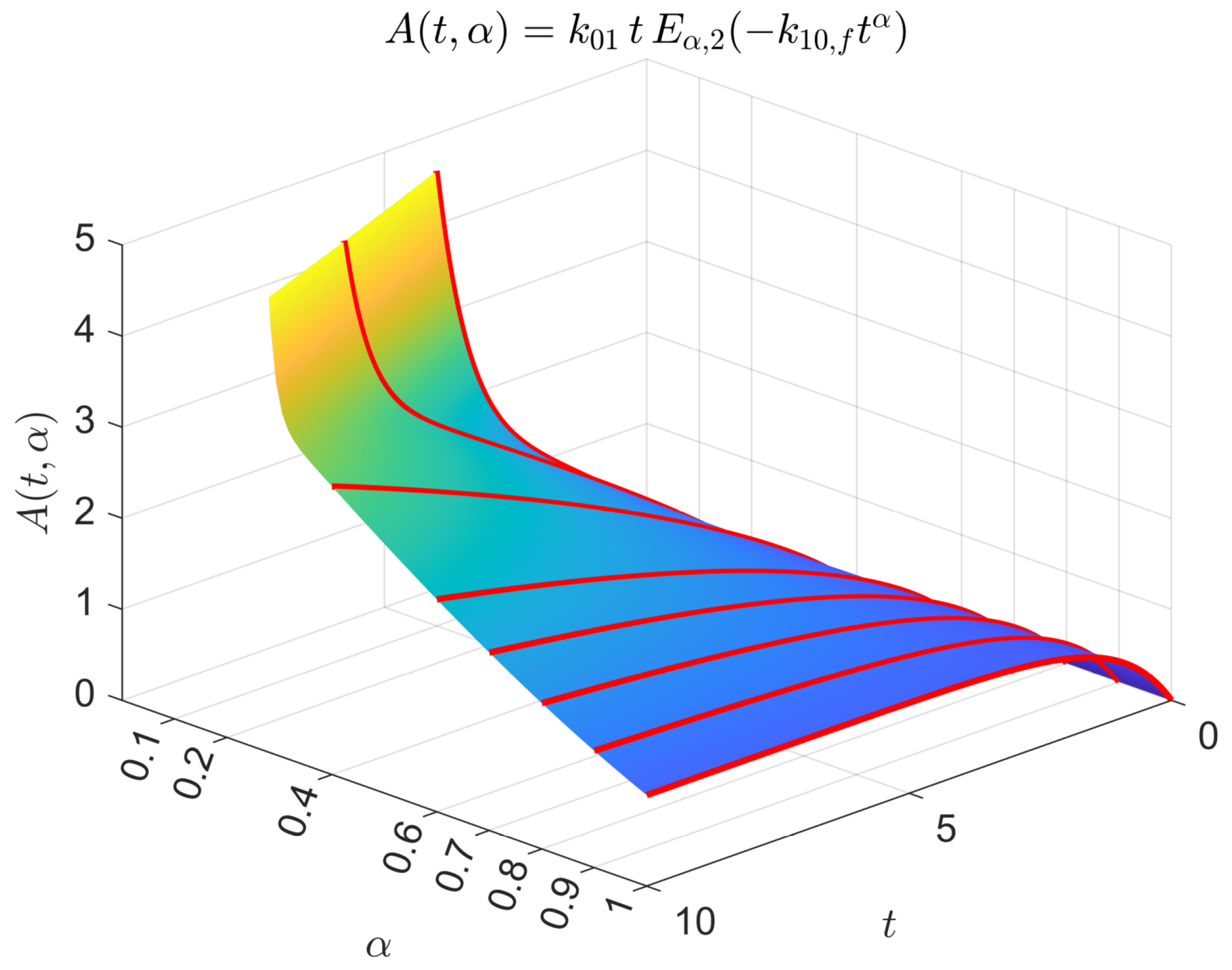
Thus, for $0<\alpha <1$ the amount $A\left(t\right)$ does not converge to a finite steady state; rather, it grows sublinearly like $t^{1-\alpha }$. This short- and long-time behavior is illustrated in Figure 1, which displays the surface $(t,\alpha )\mapsto A(t,\alpha )$ together with selected trajectories (for fixed $\alpha$) highlighted as red curves.

However, for the flux–fractional formulation (Equation (19)), it is more natural to focus on the fractional flux and to seek an appropriate notion of fractional “steady balance”. The fractional flux associated with Equation (19) is defined by

$$(\mathrm{fractional}\mathrm{flux})\left(t\right):={}^{\mathrm{C}}D_{0+}^{1-\alpha }A\left(t\right).$$

(26)

Using the explicit solution of Equation (23), given by Equation (25), we therefore need to compute the Caputo derivative ${}^{\mathrm{C}}D_{0+}^{1-\alpha }$ of the function $t\mapsto t{E}_{\alpha ,2}(-k_{10,f}{t}^{\alpha })$.

To this end we recall a standard identity for the Riemann–Liouville fractional derivative of Mittag–Leffler-type functions (see, e.g., Equation (1.82) [3]): for $0<\mu <1$, $\beta >\mu$ and $\alpha >0$,

$$\left(D_{0+}^{\mu }\left[t^{\beta -1}{E}_{\alpha ,\beta }\left(\lambda t^{\alpha }\right)\right]\right)\left(t\right)=t^{\beta -\mu -1}{E}_{\alpha ,\beta -\mu }\left(\lambda t^{\alpha }\right),$$

(27)

where $D_{0+}^{\mu }$ denotes the Riemann–Liouville derivative of order $\mu$. In our case we have $A\left(0\right)=0$, and we use a derivative of order $0<\mu =1-\alpha <1$. Then the Riemann-Liouville and Caputo derivatives coincide, so $\left(D_{0+}^{\mu }A\right)\left(t\right)={}^{\mathrm{C}}D_{0+}^{\mu }A\left(t\right)$. In our case we take

$$\mu =1-\alpha ,\beta =2,\lambda =-k_{10,f},$$

so that $t^{\beta -1}{E}_{\alpha ,\beta }\left(\lambda t^{\alpha }\right)=t{E}_{\alpha ,2}(-k_{10,f}{t}^{\alpha })$. Substituting these parameters into Equation (27) yields

$${}^{\mathrm{C}}D_{0+}^{1-\alpha }\left[t{E}_{\alpha ,2}(-k_{10,f}{t}^{\alpha })\right]=t^{2-(1-\alpha )-1}{E}_{\alpha ,2-(1-\alpha )}(-k_{10,f}{t}^{\alpha })=t^{\alpha }{E}_{\alpha ,1+\alpha }(-k_{10,f}{t}^{\alpha }).$$

Multiplying by the factor $k_{01}$ from Equation (25), we obtain the explicit expression

$${}^{\mathrm{C}}D_{0+}^{1-\alpha }A\left(t\right)=k_{01}{t}^{\alpha }{E}_{\alpha ,1+\alpha }(-k_{10,f}{t}^{\alpha }),$$

(28)

for the fractional flux in the flux–fractional formulation (Equation (19)).

Using the large-argument asymptotics of the Mittag–Leffler function, we recall that for $0<\alpha <2$, $\beta >\alpha$ and $x\to \infty$ one has (see, e.g., Section 1.3 [3], Section 1.3 [16])

$$E_{\alpha ,\beta }(-x)\sim {\displaystyle \sum _{m=1}^{\infty }}{\displaystyle \frac{{(-1)}^{m+1}}{x^m\Gamma (\beta -\alpha m)}}.$$

(29)

In particular, for $\beta =1+\alpha$ the first term ($m=1$) in Equation (29) gives

$$E_{\alpha ,1+\alpha }(-x)\sim {\displaystyle \frac{1}{x\Gamma (1+\alpha -\alpha )}}={\displaystyle \frac{1}{x\Gamma \left(1\right)}}={\displaystyle \frac{1}{x}},x\to \infty ,$$

so that

$$E_{\alpha ,1+\alpha }(-x)={\displaystyle \frac{1}{x}}+\mathcal{O}\left({\displaystyle \frac{1}{x^2}}\right),x\to \infty .$$

(30)

Setting $x=k_{10,f}{t}^{\alpha }$ in Equation (30), we obtain

$$E_{\alpha ,1+\alpha }(-k_{10,f}{t}^{\alpha })={\displaystyle \frac{1}{k_{10,f}{t}^{\alpha }}}+\mathcal{O}\left({\displaystyle \frac{1}{t^{2\alpha }}}\right),t\to \infty .$$

Multiplying by $t^{\alpha }$ yields

$$t^{\alpha }{E}_{\alpha ,1+\alpha }(-k_{10,f}{t}^{\alpha })={\displaystyle \frac{1}{k_{10,f}}}+\mathcal{O}\left({\displaystyle \frac{1}{t^{\alpha }}}\right),t\to \infty ,$$

and hence

$$t^{\alpha }{E}_{\alpha ,1+\alpha }(-k_{10,f}{t}^{\alpha })⟶{\displaystyle \frac{1}{k_{10,f}}}(t\to \infty ).$$

and therefore

$${}^{\mathrm{C}}D_{0+}^{1-\alpha }A\left(t\right)⟶{\displaystyle \frac{k_{01}}{k_{10,f}}}(t\to \infty ).$$

Equivalently, from Equation (19) one has

$$k_{01}-k_{10,f}{}^{\mathrm{C}}D_{0+}^{1-\alpha }A\left(t\right)\to 0(t\to \infty ),$$

so the right-hand side tends to zero and the input and fractional elimination fluxes balance asymptotically. In this sense the flux reaches a fractional “steady balance” even though the state variable $A\left(t\right)$ itself does not settle at a constant level.

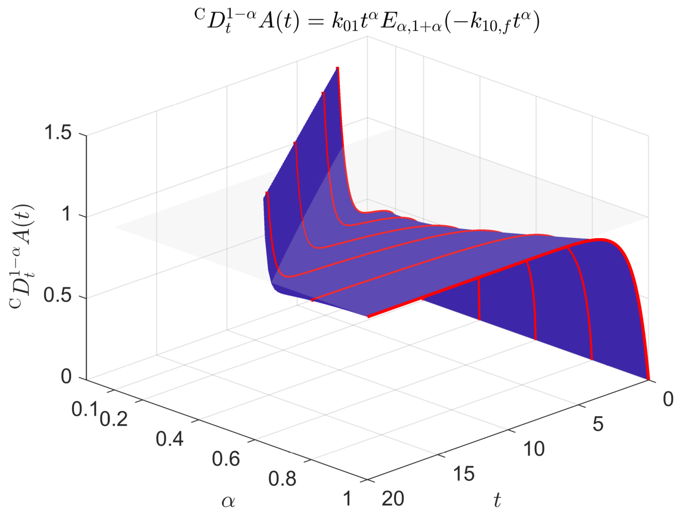
This behavior is illustrated in Figure 2, which shows the surface

$$(t,\alpha )⟼{}^{\mathrm{C}}D_{0+}^{1-\alpha }A\left(t\right)=k_{01}{t}^{\alpha }{E}_{\alpha ,1+\alpha }(-k_{10,f}{t}^{\alpha }),0<\alpha \le 1,$$

together with a horizontal plane at height $k_{01}/k_{10,f}$. For each fixed $\alpha$, the corresponding trajectory (highlighted as a red curve on the surface) rises from zero and approaches this plane, making the asymptotic flux limit $k_{01}/k_{10,f}$ visible across all fractional orders.

In the classical case $\alpha =1$ the situation changes qualitatively. One has

$$E_{1,2}\left(z\right)={\displaystyle \frac{e^z-1}{z}},$$

and the solution reduces to

$$A\left(t\right)=k_{01}t{E}_{1,2}(-k_{10,f}t)={\displaystyle \frac{k_{01}}{k_{10,f}}}\left(1-e^{-k_{10,f}t}\right),$$

which coincides with the standard one-compartment model with first-order elimination and constant rate input. Taking $t\to \infty$ gives the usual steady state

$$A_{\infty }=\underset{t\to \infty }{lim}A\left(t\right)={\displaystyle \frac{k_{01}}{k_{10,f}}},$$

and in this classical ODE setting flux balance and a constant steady state coincide.

In the opposite limit $\alpha \to 0^{+}$, using Equation (25) together with the Laplace-transform formula for $t^{\alpha }{E}_{\alpha ,1+\alpha }(-k_{10,f}{t}^{\alpha })$, one finds that for each fixed $t>0$,

$$t^{\alpha }{E}_{\alpha ,1+\alpha }(-k_{10,f}{t}^{\alpha })⟶{\displaystyle \frac{1}{1+k_{10,f}}}(\alpha \to 0^{+}),$$

and hence

$${}^{\mathrm{C}}D_{0+}^{1-\alpha }A\left(t\right)=k_{01}{t}^{\alpha }{E}_{\alpha ,1+\alpha }(-k_{10,f}{t}^{\alpha })⟶{\displaystyle \frac{k_{01}}{1+k_{10,f}}}(\alpha \to 0^{+}).$$

In other words, as $\alpha \to 0^{+}$ the fractional flux approaches the constant value

$${\displaystyle \frac{k_{01}}{1+k_{10,f}}},$$

and the state approaches the linear growth law

$$A\left(t\right)={\displaystyle \frac{k_{01}}{1+k_{10,f}}}t,t\ge 0.$$

This function solves the limiting first-order balance

$$(1+k_{10,f}){\displaystyle \frac{dA}{dt}}\left(t\right)=k_{01},A\left(0\right)=0.$$

Remark 1

(On the boundary case $\alpha \to 0^{+}$). Our formulation is intended for $0<\alpha \le 1$, and we do not regard $\alpha =0$ as an admissible model parameter. Nevertheless, the formal limit $\alpha \to 0^{+}$ is informative for the interpretation of the flux–fractional model. In this limit the order $1-\alpha$ of the Caputo derivative in Equation (19) tends to 1, and the explicit flux expression (Equation (28)) shows that, for each fixed $t>0$,

$${}^{\mathrm{C}}D_{0+}^{1-\alpha }A\left(t\right)=k_{01}{t}^{\alpha }{E}_{\alpha ,1+\alpha }(-k_{10,f}{t}^{\alpha })⟶{\displaystyle \frac{k_{01}}{1+k_{10,f}}}(\alpha \to 0^{+}).$$

Thus the family of fractional models connects continuously, at the boundary $\alpha \to 0^{+}$, to a degenerate classical first-order balance in which the flux is (approximately) constant and the amount grows essentially linearly in time. This limiting case is best viewed as a consistency check on the fractional formulation rather than as a physically meaningful choice of α.

In what follows, the flux–fractional formulation (Equation (19)) is adopted, as it extends naturally to multi-compartment systems.

3. State Sensitivity System: Functional Setting

3.1. State Sensitivity System and Classical Relative Sensitivities

We consider the forced flux–fractional m-compartment model

$$\dot{q}\left(t\right)=\mathbf{A}(\theta ,\alpha )q\left(t\right)+\mathbf{B}(\theta ,\alpha ){}^{\mathrm{C}}D_{0+}^{1-\alpha }q\left(t\right)+b(t,\theta ,\alpha ),q\left(0\right)=q_0(\theta ,\alpha ),$$

(31)

where $0<\alpha <1$, $q:[0,T]\to {\mathbb{R}}^m$, and ${}^{\mathrm{C}}D_{0+}^{1-\alpha }$ denotes the Caputo fractional derivative acting componentwise. The parameter vector is

$$\theta ={\left({\theta }_j\right)}_{1\le j\le p_{\theta }}^{\top }\in {\mathbb{R}}^{p_{\theta }}.$$

The matrices

$$\mathbf{A}=\mathbf{A}(\theta ,\alpha ),\mathbf{B}=\mathbf{B}(\theta ,\alpha )$$

belong to ${\mathbb{R}}^{m\times m}$, while

$$b(·,\theta ,\alpha ):[0,T]\to {\mathbb{R}}^m$$

is a prescribed external input. When differentiating with respect to the classical parameter vector $\theta$, the fractional order $\alpha$ is regarded as fixed.

The mathematical assumptions used below are those required for the well-posedness and differentiability analysis and are distinguished from the additional structural restrictions associated with a particular pharmacokinetic interpretation. In a compartmental model, $\mathbf{A}$ represents classical intercompartmental transfer and elimination contributions, $\mathbf{B}$ represents fluxes carrying fractional-memory effects, and b accounts for external input. Further details concerning the pharmacokinetic interpretation, dimensional consistency, and compartmental balance structure can be found in [5,6].

The inclusion of the forcing term b is essential for compartment models with external input. In particular, the one-compartment flux–fractional model introduced in Equation (19),

$${\displaystyle \frac{dA}{dt}}\left(t\right)=k_{01}-k_{10,f}{}^{\mathrm{C}}D_{0+}^{1-\alpha }A\left(t\right),A\left(0\right)=0,$$

is recovered from Equation (31) by taking

$$m=1,\mathbf{A}(\theta ,\alpha )=0,\mathbf{B}(\theta ,\alpha )=-k_{10,f},b(t,\theta ,\alpha )=k_{01},$$

with

$$\theta ={(k_{01},k_{10,f})}^{\top }.$$

For each parameter ${\theta }_j$, $j=1,\dots ,p_{\theta }$, we define the state sensitivity by

$$S_j\left(t\right):={\partial }_{{\theta }_j}q(t,\theta ,\alpha )\in {\mathbb{R}}^m.$$

At this stage, the differentiation is understood formally; its rigorous justification as differentiation of the solution map will be established below.

Differentiating Equation (31) with respect to ${\theta }_j$, with $\alpha$ fixed, gives

$$\begin{array}{cc}\hfill {\dot{S}}_j\left(t\right)& =\mathbf{A}(\theta ,\alpha )S_j\left(t\right)+\mathbf{B}(\theta ,\alpha ){}^{\mathrm{C}}D_{0+}^{1-\alpha }{S}_j\left(t\right)\hfill \\ \hfill & +{\partial }_{{\theta }_j}\mathbf{A}(\theta ,\alpha )q\left(t\right)+{\partial }_{{\theta }_j}\mathbf{B}(\theta ,\alpha ){}^{\mathrm{C}}D_{0+}^{1-\alpha }q\left(t\right)+{\partial }_{{\theta }_j}b(t,\theta ,\alpha ),\hfill \end{array}$$

(32)

for $j=1,\dots ,p_{\theta }$.

The corresponding initial condition is

$$S_j\left(0\right)={\partial }_{{\theta }_j}{q}_0(\theta ,\alpha ),j=1,\dots ,p_{\theta }.$$

(33)

We collect the classical parameter sensitivities into

$$s_{\theta }\left(t\right):={\left(S_1{\left(t\right)}^{\top },\dots ,S_{p_{\theta }}{\left(t\right)}^{\top }\right)}^{\top }\in {\mathbb{R}}^{m{p}_{\theta }},$$

and introduce the combined state–sensitivity vector

$$z_{\theta }\left(t\right):={\left(q{\left(t\right)}^{\top },S_1{\left(t\right)}^{\top },\dots ,S_{p_{\theta }}{\left(t\right)}^{\top }\right)}^{\top }\in {\mathbb{R}}^{m(p_{\theta }+1)}.$$

The Caputo derivative of $z_{\theta }$ is understood componentwise:

$${}^{\mathrm{C}}D_{0+}^{1-\alpha }{z}_{\theta }\left(t\right)={\left({\left({}^{\mathrm{C}}D_{0+}^{1-\alpha }q\left(t\right)\right)}^{\top },{\left({}^{\mathrm{C}}D_{0+}^{1-\alpha }{S}_1\left(t\right)\right)}^{\top },\dots ,{\left({}^{\mathrm{C}}D_{0+}^{1-\alpha }{S}_{p_{\theta }}\left(t\right)\right)}^{\top }\right)}^{\top }.$$

Define the block matrices

$${\mathcal{A}}_{\theta }=\left(\begin{array}{cccc}\mathbf{A}& 0& \dots & 0\\ {\partial }_{{\theta }_1}\mathbf{A}& \mathbf{A}& \dots & 0\\ ⋮& ⋮& \ddots & ⋮\\ {\partial }_{{\theta }_{p_{\theta }}}\mathbf{A}& 0& \dots & \mathbf{A}\end{array}\right),$$

and

$${\mathcal{B}}_{\theta }=\left(\begin{array}{cccc}\mathbf{B}& 0& \dots & 0\\ {\partial }_{{\theta }_1}\mathbf{B}& \mathbf{B}& \dots & 0\\ ⋮& ⋮& \ddots & ⋮\\ {\partial }_{{\theta }_{p_{\theta }}}\mathbf{B}& 0& \dots & \mathbf{B}\end{array}\right).$$

We also introduce the augmented forcing vector

$${\mathfrak{b}}_{\theta }\left(t\right):=\left(\begin{array}{c}b(t,\theta ,\alpha )\\ {\partial }_{{\theta }_1}b(t,\theta ,\alpha )\\ ⋮\\ {\partial }_{{\theta }_{p_{\theta }}}b(t,\theta ,\alpha )\end{array}\right)\in {\mathbb{R}}^{m(p_{\theta }+1)}.$$

(34)

Then the state equation and the classical parameter sensitivity equations can be written as the single forced system

$${\dot{z}}_{\theta }\left(t\right)={\mathcal{A}}_{\theta }{z}_{\theta }\left(t\right)+{\mathcal{B}}_{\theta }{}^{\mathrm{C}}D_{0+}^{1-\alpha }{z}_{\theta }\left(t\right)+{\mathfrak{b}}_{\theta }\left(t\right).$$

(35)

The initial condition is

$$z_{\theta }\left(0\right)={\left(q_0{(\theta ,\alpha )}^{\top },{\left({\partial }_{{\theta }_1}{q}_0(\theta ,\alpha )\right)}^{\top },\dots ,{\left({\partial }_{{\theta }_{p_{\theta }}}{q}_0(\theta ,\alpha )\right)}^{\top }\right)}^{\top }.$$

(36)

For the one-compartment model, with

$${\theta }_1=k_{01},{\theta }_2=k_{10,f},$$

we have

$${\partial }_{k_{01}}b=1,{\partial }_{k_{10,f}}b=0,{\partial }_{k_{01}}\mathbf{B}=0,{\partial }_{k_{10,f}}\mathbf{B}=-1.$$

Consequently, Equation (32) gives

$${\displaystyle \frac{d}{dt}}\left({\displaystyle \frac{\partial A}{\partial k_{01}}}\right)=1-k_{10,f}{}^{\mathrm{C}}D_{0+}^{1-\alpha }\left({\displaystyle \frac{\partial A}{\partial k_{01}}}\right),$$

and

$${\displaystyle \frac{d}{dt}}\left({\displaystyle \frac{\partial A}{\partial k_{10,f}}}\right)=-{}^{\mathrm{C}}D_{0+}^{1-\alpha }A\left(t\right)-k_{10,f}{}^{\mathrm{C}}D_{0+}^{1-\alpha }\left({\displaystyle \frac{\partial A}{\partial k_{10,f}}}\right),$$

which are precisely the two classical parameter-sensitivity equations associated with the one-compartment model.

We next define the relative sensitivities. Fix $t>0$ and a nominal parameter vector $\overline{\theta }\in {\mathbb{R}}^{p_{\theta }}$, and assume that ${\overline{\theta }}_j\ne 0$ and $q_i(t,\overline{\theta },\alpha )\ne 0$ for some $i\in \{1,\dots ,m\}$ and $j\in \{1,\dots ,p_{\theta }\}$.

Let

$$\mathsf{S}(t,\theta ,\alpha ):=\left(\begin{array}{cccc}{\partial }_{{\theta }_1}q(t,\theta ,\alpha )& {\partial }_{{\theta }_2}q(t,\theta ,\alpha )& \dots & {\partial }_{{\theta }_{p_{\theta }}}q(t,\theta ,\alpha )\end{array}\right)\in {\mathbb{R}}^{m\times p_{\theta }}$$

denote the state sensitivity matrix. Writing ${\mathsf{S}}_{ij}(t,\overline{\theta },\alpha )$ for its $(i,j)$-entry, we define the relative sensitivity of $q_i$ with respect to ${\theta }_j$ by

$${\sigma }_{q_i,{\theta }_j}(t;\overline{\theta },\alpha ):={\displaystyle \frac{{\overline{\theta }}_j}{q_i(t,\overline{\theta },\alpha )}}{\mathsf{S}}_{ij}(t,\overline{\theta },\alpha )={\displaystyle \frac{{\overline{\theta }}_j}{q_i(t,\overline{\theta },\alpha )}}{\displaystyle \frac{\partial q_i}{\partial {\theta }_j}}(t,\overline{\theta },\alpha ).$$

(37)

The quantity in Equation (37) is dimensionless and therefore provides a natural scale-independent measure for comparing the influence of the classical model parameters on compartment amounts or concentrations.

In addition to the parameter vector $\theta$, we consider the dependence of the state on the fractional order $\alpha \in (0,1)$. The differentiation with respect to $\alpha$ requires some care because the order enters the Caputo kernel and, in flux–fractional models, also affects the physical dimension of the corresponding fractional rate coefficient.

To formulate the order sensitivity without changing the dimensional time variable, we fix a reference time $t_{*}>0$, having the same physical unit as t. For a fractional coefficient with dimension $T^{-\alpha }$, such as $k_{10,f}$ in the one-compartment model, we regard the dimensionless combination

$$\kappa :=k_{10,f}{t}_{*}^{\alpha }$$

as fixed when $\alpha$ varies. Equivalently,

$$k_{10,f}\left(\alpha \right)=\kappa t_{*}^{-\alpha },{\partial }_{\alpha }{k}_{10,f}\left(\alpha \right)=-(ln{t}_{*})k_{10,f}\left(\alpha \right).$$

Thus, the meaning of differentiation with respect to $\alpha$ is fixed independently of the particular choice of time units.

We define the fractional-order sensitivity by

$$S_{\alpha }\left(t\right):={\partial }_{\alpha }q(t,\theta ,\alpha )\in {\mathbb{R}}^m.$$

For convenience, set

$${\mathcal{D}}_{\alpha }:={}^{\mathrm{C}}D_{0+}^{1-\alpha }.$$

When differentiating ${\mathcal{D}}_{\alpha }q$, it is important to distinguish the dependence of the operator on $\alpha$ from the dependence of the state q on $\alpha$. We therefore define

$$\left({\partial }_{\alpha }^{\mathrm{op}}{\mathcal{D}}_{\alpha }\right)q:={\left.{\displaystyle \frac{\partial }{\partial \alpha }}\left({\mathcal{D}}_{\alpha }v\right)\right|}_{v=q},$$

where q is held fixed in the differentiation. Consequently,

$${\partial }_{\alpha }\left({\mathcal{D}}_{\alpha }q\right)={\mathcal{D}}_{\alpha }{S}_{\alpha }+\left({\partial }_{\alpha }^{\mathrm{op}}{\mathcal{D}}_{\alpha }\right)q.$$

(38)

Using the representation

$${\mathcal{D}}_{\alpha }q\left(t\right)={\displaystyle \frac{1}{\Gamma \left(\alpha \right)}}{\int }_0^t{(t-\tau )}^{\alpha -1}\dot{q}\left(\tau \right)d\tau ,$$

differentiation of the operator with the state held fixed gives

$$\left({\partial }_{\alpha }^{\mathrm{op}}{\mathcal{D}}_{\alpha }\right)q\left(t\right)={\displaystyle \frac{1}{\Gamma \left(\alpha \right)}}{\int }_0^t{(t-\tau )}^{\alpha -1}\left[ln(t-\tau )-\psi \left(\alpha \right)\right]\dot{q}\left(\tau \right)d\tau ,$$

(39)

where

$$\psi \left(\alpha \right):={\displaystyle \frac{{\Gamma }^{\prime }\left(\alpha \right)}{\Gamma \left(\alpha \right)}}$$

is the digamma function.

The expression in Equation (39) is the derivative of the fractional operator itself. In a flux term whose coefficient has dimension $T^{-\alpha }$, the derivative of that coefficient combines with Equation (39). Indeed, if

$$\mathbf{B}(\theta ,\alpha )=\mathcal{K}\left(\theta \right)t_{*}^{-\alpha },$$

with $\mathcal{K}\left(\theta \right)$ fixed when $\alpha$ varies, then

$${\partial }_{\alpha }\mathbf{B}(\theta ,\alpha )=-(ln{t}_{*})\mathbf{B}(\theta ,\alpha ).$$

Hence

$$\begin{array}{cc}\hfill & {\partial }_{\alpha }\left(\mathbf{B}(\theta ,\alpha ){}^{\mathrm{C}}D_{0+}^{1-\alpha }q\right)\hfill \\ \hfill & =\mathbf{B}(\theta ,\alpha ){}^{\mathrm{C}}D_{0+}^{1-\alpha }{S}_{\alpha }+\mathbf{B}(\theta ,\alpha ){}^{\mathrm{C}}D_{0+}^{1-\alpha ,ln,t_{*}}q,\hfill \end{array}$$

(40)

where we define the reference-time logarithmic Caputo-type operator by

$${}^{\mathrm{C}}D_{0+}^{1-\alpha ,ln,t_{*}}q\left(t\right):={\displaystyle \frac{1}{\Gamma \left(\alpha \right)}}{\int }_0^t{(t-\tau )}^{\alpha -1}\left[ln\left({\displaystyle \frac{t-\tau }{t_{*}}}\right)-\psi \left(\alpha \right)\right]\dot{q}\left(\tau \right)d\tau .$$

(41)

The logarithm in Equation (41) is dimensionless, since $(t-\tau )/t_{*}$ is a ratio of two quantities having the same physical unit.

Equivalently, introducing the kernel

$$k_{\alpha ,t_{*}}\left(t\right):={\displaystyle \frac{1}{\Gamma \left(\alpha \right)}}{t}^{\alpha -1}\left[ln\left({\displaystyle \frac{t}{t_{*}}}\right)-\psi \left(\alpha \right)\right],t>0,$$

(42)

we have

$${}^{\mathrm{C}}D_{0+}^{1-\alpha ,ln,t_{*}}q=k_{\alpha ,t_{*}}\ast \dot{q}.$$

We now differentiate the forced state Equation (31). In its most general form, allowing $\mathbf{A}$, $\mathbf{B}$, and b to possess an explicit dependence on $\alpha$, one obtains

$$\begin{array}{cc}\hfill {\dot{S}}_{\alpha }\left(t\right)& =\mathbf{A}{S}_{\alpha }\left(t\right)+\mathbf{B}{}^{\mathrm{C}}D_{0+}^{1-\alpha }{S}_{\alpha }\left(t\right)\hfill \\ \hfill & +\left({\partial }_{\alpha }\mathbf{A}\right)q\left(t\right)+\left({\partial }_{\alpha }\mathbf{B}\right){}^{\mathrm{C}}D_{0+}^{1-\alpha }q\left(t\right)\hfill \\ \hfill & +\mathbf{B}\left({\partial }_{\alpha }^{\mathrm{op}}{\mathcal{D}}_{\alpha }\right)q\left(t\right)+{\partial }_{\alpha }b(t,\theta ,\alpha ).\hfill \end{array}$$

(43)

When $\mathbf{A}$ has no explicit $\alpha$-dependence and

$$\mathbf{B}(\theta ,\alpha )=\mathcal{K}\left(\theta \right)t_{*}^{-\alpha },$$

with $\mathcal{K}\left(\theta \right)$ fixed when $\alpha$ varies, the two terms involving ${\partial }_{\alpha }\mathbf{B}$ and ${\partial }_{\alpha }^{\mathrm{op}}{\mathcal{D}}_{\alpha }$ combine according to Equation (40). Therefore,

$${\dot{S}}_{\alpha }\left(t\right)=\mathbf{A}{S}_{\alpha }\left(t\right)+\mathbf{B}{}^{\mathrm{C}}D_{0+}^{1-\alpha }{S}_{\alpha }\left(t\right)+\mathbf{B}{}^{\mathrm{C}}D_{0+}^{1-\alpha ,ln,t_{*}}q\left(t\right)+{\partial }_{\alpha }b(t,\theta ,\alpha ).$$

(44)

If the prescribed input does not depend explicitly on $\alpha$, then ${\partial }_{\alpha }b=0$, and Equation (44) reduces to

$${\dot{S}}_{\alpha }\left(t\right)=\mathbf{A}{S}_{\alpha }\left(t\right)+\mathbf{B}{}^{\mathrm{C}}D_{0+}^{1-\alpha }{S}_{\alpha }\left(t\right)+\mathbf{B}{}^{\mathrm{C}}D_{0+}^{1-\alpha ,ln,t_{*}}q\left(t\right).$$

(45)

If the initial condition $q_0(\theta ,\alpha )$ depends on $\alpha$, then

$$S_{\alpha }\left(0\right)={\partial }_{\alpha }{q}_0(\theta ,\alpha ).$$

In particular, when the initial condition is independent of $\alpha$,

$$S_{\alpha }\left(0\right)=0.$$

For the one-compartment model,

$${\displaystyle \frac{dA}{dt}}=k_{01}-k_{10,f}{}^{\mathrm{C}}D_{0+}^{1-\alpha }A,$$

we hold

$$\kappa =k_{10,f}{t}_{*}^{\alpha }$$

fixed when differentiating with respect to $\alpha$. Since $k_{01}$ has the fixed physical dimension of an input rate and is independent of $\alpha$, the order sensitivity satisfies

$${\displaystyle \frac{d{S}_{\alpha }}{dt}}\left(t\right)=-k_{10,f}{}^{\mathrm{C}}D_{0+}^{1-\alpha }{S}_{\alpha }\left(t\right)-k_{10,f}{}^{\mathrm{C}}D_{0+}^{1-\alpha ,ln,t_{*}}A\left(t\right),S_{\alpha }\left(0\right)=0.$$

(46)

For the augmented formulation below, we specialize to the case in which $\mathbf{A}$ has no explicit dependence on $\alpha$ and

$$\mathbf{B}(\theta ,\alpha )=\mathcal{K}\left(\theta \right)t_{*}^{-\alpha },$$

with $\mathcal{K}\left(\theta \right)$ fixed when $\alpha$ varies.

We next combine the state and its sensitivities. Let

$$s_{\theta }\left(t\right):={\left(S_1{\left(t\right)}^{\top },\dots ,S_{p_{\theta }}{\left(t\right)}^{\top }\right)}^{\top }\in {\mathbb{R}}^{m{p}_{\theta }},$$

and define

$$z\left(t\right):={\left(q{\left(t\right)}^{\top },s_{\theta }{\left(t\right)}^{\top },S_{\alpha }{\left(t\right)}^{\top }\right)}^{\top }\in {\mathbb{R}}^{m(p_{\theta }+2)}.$$

(47)

The Caputo derivative of z is understood componentwise:

$${}^{\mathrm{C}}D_{0+}^{1-\alpha }z\left(t\right):={\left({\left({}^{\mathrm{C}}D_{0+}^{1-\alpha }q\left(t\right)\right)}^{\top },{\left({}^{\mathrm{C}}D_{0+}^{1-\alpha }{s}_{\theta }\left(t\right)\right)}^{\top },{\left({}^{\mathrm{C}}D_{0+}^{1-\alpha }{S}_{\alpha }\left(t\right)\right)}^{\top }\right)}^{\top }.$$

With the notation introduced above, the state equation, the classical parameter-sensitivity equations, and the fractional-order sensitivity equation may be collected into

$$\dot{z}\left(t\right)={\mathcal{A}}_{p_{\theta }+2}z\left(t\right)+{\mathcal{B}}_{p_{\theta }+2}{}^{\mathrm{C}}D_{0+}^{1-\alpha }z\left(t\right)+\mathfrak{b}\left(t\right)+\mathcal{C}{}^{\mathrm{C}}D_{0+}^{1-\alpha ,ln,t_{*}}z\left(t\right),$$

(48)

where

$${\mathcal{A}}_{p_{\theta }+2}=\left(\begin{array}{ccccc}\mathbf{A}& 0& \dots & 0& 0\\ {\partial }_{{\theta }_1}\mathbf{A}& \mathbf{A}& \dots & 0& 0\\ ⋮& ⋮& \ddots & ⋮& ⋮\\ {\partial }_{{\theta }_{p_{\theta }}}\mathbf{A}& 0& \dots & \mathbf{A}& 0\\ 0& 0& \dots & 0& \mathbf{A}\end{array}\right),$$

$${\mathcal{B}}_{p_{\theta }+2}=\left(\begin{array}{ccccc}\mathbf{B}& 0& \dots & 0& 0\\ {\partial }_{{\theta }_1}\mathbf{B}& \mathbf{B}& \dots & 0& 0\\ ⋮& ⋮& \ddots & ⋮& ⋮\\ {\partial }_{{\theta }_{p_{\theta }}}\mathbf{B}& 0& \dots & \mathbf{B}& 0\\ 0& 0& \dots & 0& \mathbf{B}\end{array}\right).$$

The matrix $\mathcal{C}$ contains only the coupling of the state to the fractional-order sensitivity equation:

$$\mathcal{C}=\left(\begin{array}{ccccc}0& 0& \dots & 0& 0\\ 0& 0& \dots & 0& 0\\ ⋮& ⋮& \ddots & ⋮& ⋮\\ 0& 0& \dots & 0& 0\\ \mathbf{B}& 0& \dots & 0& 0\end{array}\right).$$

The prescribed forcing term is

$$\mathfrak{b}\left(t\right):=\left(\begin{array}{c}b(t,\theta ,\alpha )\\ {\partial }_{{\theta }_1}b(t,\theta ,\alpha )\\ ⋮\\ {\partial }_{{\theta }_{p_{\theta }}}b(t,\theta ,\alpha )\\ {\partial }_{\alpha }b(t,\theta ,\alpha )\end{array}\right).$$

(49)

The initial condition for Equation (48) is

$$z\left(0\right)={\left(q_0^{\top },{\left({\partial }_{{\theta }_1}{q}_0\right)}^{\top },\dots ,{\left({\partial }_{{\theta }_{p_{\theta }}}{q}_0\right)}^{\top },{\left({\partial }_{\alpha }{q}_0\right)}^{\top }\right)}^{\top }.$$

Thus, the augmented formulation separates the prescribed forcing $\mathfrak{b}$ from the logarithmic Volterra coupling represented by $\mathcal{C}$. In particular, the logarithmic term is not treated as an external forcing, since it depends on the unknown state itself. This formulation will be used in the Sobolev-space analysis below.

3.2. Sobolev Setting and Volterra Formulation

Fix $T>0$ and $1<p<\infty$, and let $(H,\parallel ·{\parallel }_H)$ be a finite-dimensional real Hilbert space. We work with the Lebesgue and Sobolev spaces

$$L^p(0,T;H)=\left\{z:(0,T)\to H:{\int }_0^T{\parallel z\left(t\right)\parallel }_H^{p}dt<\infty \right\},$$

and

$$W^{1,p}(0,T;H)=\left\{z\in L^p(0,T;H):\dot{z}\in L^p(0,T;H)\right\}.$$

equipped with the standard Sobolev norm

$${\parallel z\parallel }_{W^{1,p}(0,T;H)}^p={\parallel z\parallel }_{L^p(0,T;H)}^p+{\parallel \dot{z}\parallel }_{L^p(0,T;H)}^p.$$

(50)

Since the time interval is one-dimensional and finite, every $z\in W^{1,p}(0,T;H)$ admits a continuous representative, and the embedding

$$W^{1,p}(0,T;H)\hookrightarrow C([0,T];H)$$

is continuous. In particular, the initial trace $z\left(0\right)\in H$ is well defined.

For the augmented state–sensitivity system (Equation (48)), we take $H={\mathbb{R}}^{m(p_{\theta }+2)}$ equipped with the Euclidean norm, and all fractional operators are understood componentwise.

Lemma 2

(Caputo mapping from $W^{1,p}$ into $L^p$). Let $0<\alpha <1$, $1<p<\infty$, and $z\in W^{1,p}(0,T;H)$. Then

$${}^{\mathrm{C}}D_{0+}^{1-\alpha }z=I_{0+}^{\alpha }\dot{z}=g_{\alpha }\ast \dot{z},g_{\alpha }\left(t\right)={\displaystyle \frac{t^{\alpha -1}}{\Gamma \left(\alpha \right)}},$$

for almost every $t\in (0,T)$. Moreover,

$${∥{}^{\mathrm{C}}D_{0+}^{1-\alpha }z∥}_{L^p(0,T;H)}\le {\displaystyle \frac{T^{\alpha }}{\Gamma (\alpha +1)}}{\parallel \dot{z}\parallel }_{L^p(0,T;H)}.$$

(51)

In particular,

$${}^{\mathrm{C}}D_{0+}^{1-\alpha }\in \mathcal{L}\left(W^{1,p}(0,T;H),L^p(0,T;H)\right).$$

Proof. 

Since $0<\alpha <1$,

$${}^{\mathrm{C}}D_{0+}^{1-\alpha }z=I_{0+}^{\alpha }\dot{z}=g_{\alpha }\ast \dot{z},g_{\alpha }\left(t\right)={\displaystyle \frac{t^{\alpha -1}}{\Gamma \left(\alpha \right)}}.$$

Furthermore,

$$\parallel g_{\alpha }{\parallel }_{L^1(0,T)}={\displaystyle \frac{1}{\Gamma \left(\alpha \right)}}{\int }_0^T{t}^{\alpha -1}dt={\displaystyle \frac{T^{\alpha }}{\Gamma (\alpha +1)}}.$$

Hence, by Young’s convolution inequality,

$${∥{}^{\mathrm{C}}D_{0+}^{1-\alpha }z∥}_{L^p(0,T;H)}\le \parallel g_{\alpha }{\parallel }_{L^1(0,T)}\parallel \dot{z}{\parallel }_{L^p(0,T;H)}={\displaystyle \frac{T^{\alpha }}{\Gamma (\alpha +1)}}{\parallel \dot{z}\parallel }_{L^p(0,T;H)},$$

which proves Equation (51). Since

$$\parallel \dot{z}{\parallel }_{L^p(0,T;H)}\le {\parallel z\parallel }_{W^{1,p}(0,T;H)},$$

the asserted boundedness follows. □

Lemma 3

(Logarithmically weighted Caputo operator). Let $0<\alpha <1$, $t_{*}>0$, $1<p<\infty$, and $z\in W^{1,p}(0,T;H)$. Define

$$k_{\alpha ,t_{*}}\left(t\right):={\displaystyle \frac{t^{\alpha -1}}{\Gamma \left(\alpha \right)}}\left[ln\left({\displaystyle \frac{t}{t_{*}}}\right)-\psi \left(\alpha \right)\right],t>0.$$

(52)

Then

$$k_{\alpha ,t_{*}}\in L^1(0,T),$$

and

$${}^{\mathrm{C}}D_{0+}^{1-\alpha ,ln,t_{*}}z:=k_{\alpha ,t_{*}}\ast \dot{z}$$

belongs to $L^p(0,T;H)$. Moreover,

$${∥{}^{\mathrm{C}}D_{0+}^{1-\alpha ,ln,t_{*}}z∥}_{L^p(0,T;H)}\le \parallel k_{\alpha ,t_{*}}{\parallel }_{L^1(0,T)}{\parallel \dot{z}\parallel }_{L^p(0,T;H)}.$$

(53)

In particular,

$${}^{\mathrm{C}}D_{0+}^{1-\alpha ,ln,t_{*}}\in \mathcal{L}\left(W^{1,p}(0,T;H),L^p(0,T;H)\right).$$

Proof. 

By Equation (52),

$$|k_{\alpha ,t_{*}}\left(t\right)|\le {\displaystyle \frac{t^{\alpha -1}}{\Gamma \left(\alpha \right)}}\left(\left|ln\left({\displaystyle \frac{t}{t_{*}}}\right)\right|+\left|\psi \left(\alpha \right)\right|\right).$$

Since

$${\int }_0^T{t}^{\alpha -1}dt={\displaystyle \frac{T^{\alpha }}{\alpha }}<\infty ,$$

it remains to consider the logarithmic term. With the change in variables $t=t_{*}r$,

$${\int }_0^T{t}^{\alpha -1}\left|ln\left({\displaystyle \frac{t}{t_{*}}}\right)\right|dt=t_{*}^{\alpha }{\int }_0^{T/t_{*}}{r}^{\alpha -1}|lnr|dr.$$

Now

$${\int }_0^1{r}^{\alpha -1}|lnr|dr={\displaystyle \frac{1}{{\alpha }^2}}<\infty ,$$

whereas $r^{\alpha -1}|lnr|$ is continuous on every compact subinterval of $(0,\infty )$. Hence

$${\int }_0^{T/t_{*}}{r}^{\alpha -1}|lnr|dr<\infty ,$$

and therefore

$$k_{\alpha ,t_{*}}\in L^1(0,T).$$

Young’s convolution inequality now gives

$${∥{}^{\mathrm{C}}D_{0+}^{1-\alpha ,ln,t_{*}}z∥}_{L^p(0,T;H)}\le \parallel k_{\alpha ,t_{*}}{\parallel }_{L^1(0,T)}{\parallel \dot{z}\parallel }_{L^p(0,T;H)},$$

which proves Equation (53). Since

$$\parallel \dot{z}{\parallel }_{L^p(0,T;H)}\le {\parallel z\parallel }_{W^{1,p}(0,T;H)},$$

the asserted boundedness follows. □

The preceding lemmas show that, for every

$$z\in W^{1,p}(0,T;H),$$

both

$${}^{\mathrm{C}}D_{0+}^{1-\alpha }z\mathrm{and}{}^{\mathrm{C}}D_{0+}^{1-\alpha ,ln,t_{*}}z$$

belong to $L^p(0,T;H)$. Hence all fractional terms appearing in the augmented system (Equation (48)) are well defined in $L^p(0,T;H)$. We therefore work directly in the Sobolev space $W^{1,p}(0,T;H)$ throughout the subsequent analysis.

4. Well-Posedness on Arbitrary Finite Time Intervals

We consider the abstract augmented problem

$$\dot{z}\left(t\right)=\mathcal{A}z\left(t\right)+\mathcal{B}{}^{\mathrm{C}}D_{0+}^{1-\alpha }z\left(t\right)+\mathcal{C}{}^{\mathrm{C}}D_{0+}^{1-\alpha ,ln,t_{*}}z\left(t\right)+F\left(t\right),z\left(0\right)=z_0,$$

(54)

where

$$\mathcal{A},\mathcal{B},\mathcal{C}\in \mathcal{L}\left(H\right),z_0\in H,F\in L^p(0,T;H).$$

For the augmented state–sensitivity system (Equation (48)), the operators $\mathcal{A}$, $\mathcal{B}$, and $\mathcal{C}$ are the block operators introduced above, while $F=\mathfrak{b}$. Thus, in that case, we assume

$$\mathfrak{b}\in L^p(0,T;H).$$

Set

$$u:=\dot{z}.$$

Then

$$z\left(t\right)=z_0+{\int }_0^{t}u\left(s\right)ds=z_0+(g_1\ast u)\left(t\right),g_1\left(t\right)\equiv 1.$$

Moreover,

$${}^{\mathrm{C}}D_{0+}^{1-\alpha }z=g_{\alpha }\ast u,g_{\alpha }\left(t\right)={\displaystyle \frac{t^{\alpha -1}}{\Gamma \left(\alpha \right)}},$$

and

$${}^{\mathrm{C}}D_{0+}^{1-\alpha ,ln,t_{*}}z=k_{\alpha ,t_{*}}\ast u.$$

Hence, Equation (54) is equivalent to the Volterra equation

$$u=\mathcal{A}{z}_0+F+\mathcal{A}(g_1\ast u)+\mathcal{B}(g_{\alpha }\ast u)+\mathcal{C}(k_{\alpha ,t_{*}}\ast u)\mathrm{in}{L}^p(0,T;H).$$

(55)

For $\omega >0$, we equip $L^p(0,T;H)$ with the Bielecki norm

$${\parallel u\parallel }_{p,\omega }:={∥e^{-\omega (·)}u∥}_{L^p(0,T;H)}.$$

(56)

Since $T<\infty$, this norm is equivalent to the standard $L^p$ norm. Indeed,

$$e^{-\omega T}{\parallel u\parallel }_{L^p(0,T;H)}\le {\parallel u\parallel }_{p,\omega }\le {\parallel u\parallel }_{L^p(0,T;H)}.$$

(57)

Let $h\in L^1(0,T)$ and $u\in L^p(0,T;H)$. For almost every $t\in (0,T)$,

$$e^{-\omega t}(h\ast u)\left(t\right)={\int }_0^t{e}^{-\omega (t-s)}h(t-s)e^{-\omega s}u\left(s\right)ds.$$

Therefore, Young’s convolution inequality gives

$${\parallel h\ast u\parallel }_{p,\omega }\le {∥e^{-\omega (·)}h∥}_{L^1(0,T)}{\parallel u\parallel }_{p,\omega }.$$

(58)

Applying Equation (58) to $g_1\left(t\right)\equiv 1$, we obtain

$$\parallel g_1{\ast u\parallel }_{p,\omega }\le {\displaystyle \frac{1}{\omega }}{\parallel u\parallel }_{p,\omega },$$

(59)

since

$${\int }_0^T{e}^{-\omega t}dt={\displaystyle \frac{1-e^{-\omega T}}{\omega }}\le {\displaystyle \frac{1}{\omega }}.$$

Similarly, for

$$g_{\alpha }\left(t\right)={\displaystyle \frac{t^{\alpha -1}}{\Gamma \left(\alpha \right)}},$$

we have

$$\parallel g_{\alpha }{\ast u\parallel }_{p,\omega }\le {\omega }^{-\alpha }{\parallel u\parallel }_{p,\omega },$$

(60)

because

$${\displaystyle \frac{1}{\Gamma \left(\alpha \right)}}{\int }_0^T{e}^{-\omega t}{t}^{\alpha -1}dt\le {\displaystyle \frac{1}{\Gamma \left(\alpha \right)}}{\int }_0^{\infty }{e}^{-\omega t}{t}^{\alpha -1}dt={\omega }^{-\alpha }.$$

For the logarithmic kernel $k_{\alpha ,t_{*}}$, define

$${\eta }_{\alpha ,t_{*}}\left(\omega \right):={∥e^{-\omega (·)}{k}_{\alpha ,t_{*}}∥}_{L^1(0,T)}.$$

(61)

Then, Equation (58) yields

$$\parallel k_{\alpha ,t_{*}}{\ast u\parallel }_{p,\omega }\le {\eta }_{\alpha ,t_{*}}\left(\omega \right){\parallel u\parallel }_{p,\omega }.$$

(62)

By Lemma 3,

$$k_{\alpha ,t_{*}}\in L^1(0,T).$$

Moreover,

$$e^{-\omega t}|k_{\alpha ,t_{*}}\left(t\right)|\le |k_{\alpha ,t_{*}}\left(t\right)|\mathrm{for}t\in (0,T),$$

and, for every $t>0$,

$$e^{-\omega t}\left|k_{\alpha ,t_{*}}\left(t\right)\right|⟶0\mathrm{as}\omega \to \infty .$$

Hence, by the dominated convergence theorem,

$${\eta }_{\alpha ,t_{*}}\left(\omega \right)⟶0\mathrm{as}\omega \to \infty .$$

These estimates provide the contraction bound required to establish existence and uniqueness on any prescribed finite time interval.

Theorem 1

(Well-posedness on arbitrary finite time intervals). Let $1<p<\infty$, $0<\alpha <1$, $T>0$, and let H be a finite-dimensional real Hilbert space. Assume

$$\mathcal{A},\mathcal{B},\mathcal{C}\in \mathcal{L}\left(H\right),z_0\in H,F\in L^p(0,T;H).$$

Then the initial-value problem (Equation (54)) admits a unique solution

$$z\in W^{1,p}(0,T;H).$$

Proof. 

Define

$$\mathcal{T}:L^p(0,T;H)⟶L^p(0,T;H)$$

by

$$\mathcal{T}u:=\mathcal{A}{z}_0+F+\mathcal{A}(g_1\ast u)+\mathcal{B}(g_{\alpha }\ast u)+\mathcal{C}(k_{\alpha ,t_{*}}\ast u).$$

The map $\mathcal{T}$ is well defined. Indeed, $\mathcal{A}{z}_0$, viewed as a constant H-valued function on $(0,T)$, belongs to $L^p(0,T;H)$ since $T<\infty$, and $F\in L^p(0,T;H)$. Furthermore, the convolution estimates established above imply

$$g_1\ast u,g_{\alpha }\ast u,k_{\alpha ,t_{*}}\ast u\in L^p(0,T;H)$$

for every $u\in L^p(0,T;H)$.

For $u,v\in L^p(0,T;H)$, using Equations (59), (60) and (62), we obtain

$$\begin{array}{cc}\hfill {\parallel \mathcal{T}u-\mathcal{T}v\parallel }_{p,\omega }& \le \parallel \mathcal{A}\parallel \parallel g_1{\ast (u-v)\parallel }_{p,\omega }+\parallel \mathcal{B}\parallel \parallel g_{\alpha }{\ast (u-v)\parallel }_{p,\omega }\hfill \\ \hfill & +\parallel \mathcal{C}\parallel \parallel k_{\alpha ,t_{*}}{\ast (u-v)\parallel }_{p,\omega }\hfill \\ \hfill & \le {\rho \left(\omega \right)\parallel u-v\parallel }_{p,\omega },\hfill \end{array}$$

where

$$\rho \left(\omega \right):={\displaystyle \frac{\parallel \mathcal{A}\parallel }{\omega }}+{\displaystyle \frac{\parallel \mathcal{B}\parallel }{{\omega }^{\alpha }}}+\parallel \mathcal{C}\parallel {\eta }_{\alpha ,t_{*}}\left(\omega \right).$$

Since

$${\eta }_{\alpha ,t_{*}}\left(\omega \right)⟶0\mathrm{as}\omega \to \infty ,$$

it follows that

$$\rho \left(\omega \right)⟶0\mathrm{as}\omega \to \infty .$$

Hence one may choose $\omega >0$ such that

$$\rho \left(\omega \right)<1.$$

Thus $\mathcal{T}$ is a strict contraction on $L^p(0,T;H)$ endowed with the equivalent Bielecki norm ${\parallel ·\parallel }_{p,\omega }$.

By the Banach contraction principle, there exists a unique $u\in L^p(0,T;H)$ satisfying

$$u=\mathcal{T}u.$$

Define

$$z\left(t\right):=z_0+{\int }_0^{t}u\left(s\right)ds.$$

Then

$$z\in W^{1,p}(0,T;H),z\left(0\right)=z_0,\dot{z}=u$$

almost everywhere on $(0,T)$. Moreover,

$${}^{\mathrm{C}}D_{0+}^{1-\alpha }z=g_{\alpha }\ast u,{}^{\mathrm{C}}D_{0+}^{1-\alpha ,ln,t_{*}}z=k_{\alpha ,t_{*}}\ast u.$$

Since

$$z=z_0+g_1\ast u,$$

the fixed-point identity $u=\mathcal{T}u$ becomes

$$\dot{z}=\mathcal{A}z+\mathcal{B}{}^{\mathrm{C}}D_{0+}^{1-\alpha }z+\mathcal{C}{}^{\mathrm{C}}D_{0+}^{1-\alpha ,ln,t_{*}}z+F$$

almost everywhere on $(0,T)$. Hence, z solves Equation (54).

Finally, if $\tilde{z}\in W^{1,p}(0,T;H)$ is another solution, then $\tilde{u}:=\dot{\tilde{z}}$ satisfies the same fixed-point equation

$$\tilde{u}=\mathcal{T}\tilde{u}.$$

The uniqueness of the fixed point gives $\tilde{u}=u$, and since $\tilde{z}\left(0\right)=z\left(0\right)=z_0$, it follows that

$$\tilde{z}=z.$$

Thus the solution is unique. □

Remark 2.

Since the Bielecki norm is equivalent to the standard $L^p(0,T;H)$ norm on every finite interval, it induces the same underlying function space. Its advantage is that the exponential weight allows the Volterra operator to satisfy a contraction estimate for sufficiently large ω. Thus the fixed-point argument can be carried out without imposing any smallness condition on T or any a priori bound on the solution. Consequently, Theorem 1 yields existence and uniqueness on every prescribed finite time interval.

By Theorem 1, for every admissible $(\theta ,\alpha )$ the state equation admits a unique solution

$$q(·;\theta ,\alpha )\in W^{1,p}(0,T;{\mathbb{R}}^m).$$

We now study the dependence of this solution on the classical parameter vector $\theta$ and the fractional order $\alpha$.

Let

$$\Theta \subset {\mathbb{R}}^{p_{\theta }}$$

be open, let

$$0<{\alpha }_{-}<{\alpha }_{+}<1,$$

and fix $t_{*}>0$. Write

$$\mathbf{B}(\theta ,\alpha )=t_{*}^{-\alpha }\tilde{\mathbf{B}}(\theta ,\alpha ),$$

(63)

where $\tilde{\mathbf{B}}$ is dimensionless. Assume

$$\mathbf{A},\tilde{\mathbf{B}}\in C^1\left(\Theta \times ({\alpha }_{-},{\alpha }_{+});{\mathbb{R}}^{m\times m}\right),$$

$$q_0\in C^1\left(\Theta \times ({\alpha }_{-},{\alpha }_{+});{\mathbb{R}}^m\right),$$

and

$$b\in C^1\left(\Theta \times ({\alpha }_{-},{\alpha }_{+});L^p(0,T;{\mathbb{R}}^m)\right),$$

where differentiability of b is understood with respect to the $L^p(0,T;{\mathbb{R}}^m)$ norm.

For

$$(\theta ,\alpha )\in \Theta \times ({\alpha }_{-},{\alpha }_{+}),$$

consider

$$\dot{q}\left(t\right)=\mathbf{A}(\theta ,\alpha )q\left(t\right)+\mathbf{B}(\theta ,\alpha ){}^{\mathrm{C}}D_{0+}^{1-\alpha }q\left(t\right)+b(t,\theta ,\alpha ),q\left(0\right)=q_0(\theta ,\alpha ).$$

(64)

Set

$$u:=\dot{q},K_{1}u:=g_1\ast u,g_1\left(t\right)\equiv 1.$$

Then

$$q=q_0+K_{1}u.$$

Define

$${\tilde{g}}_{\alpha ,t_{*}}\left(t\right):=t_{*}^{-\alpha }{g}_{\alpha }\left(t\right)={\displaystyle \frac{t_{*}^{-\alpha }{t}^{\alpha -1}}{\Gamma \left(\alpha \right)}},t>0,$$

(65)

and

$${\tilde{K}}_{\alpha ,t_{*}}u:={\tilde{g}}_{\alpha ,t_{*}}\ast u.$$

Using Equation (63), we have

$$\mathbf{B}(\theta ,\alpha ){}^{\mathrm{C}}D_{0+}^{1-\alpha }q=\tilde{\mathbf{B}}(\theta ,\alpha ){\tilde{K}}_{\alpha ,t_{*}}u.$$

Hence, Equation (64) is equivalent to

$$u=F(\theta ,\alpha )+\mathbf{A}(\theta ,\alpha )K_{1}u+\tilde{\mathbf{B}}(\theta ,\alpha ){\tilde{K}}_{\alpha ,t_{*}}u,$$

(66)

where

$$F(\theta ,\alpha ):=\mathbf{A}(\theta ,\alpha )q_0(\theta ,\alpha )+b(·,\theta ,\alpha ).$$

Lemma 4

(Parameter-dependent Volterra operator). The map

$$\alpha \mapsto {\tilde{K}}_{\alpha ,t_{*}}$$

belongs to

$$C^1\left(({\alpha }_{-},{\alpha }_{+});\mathcal{L}\left(L^p(0,T;{\mathbb{R}}^m)\right)\right),$$

with

$${\partial }_{\alpha }{\tilde{g}}_{\alpha ,t_{*}}\left(t\right)={\tilde{g}}_{\alpha ,t_{*}}\left(t\right)\left[ln\left({\displaystyle \frac{t}{t_{*}}}\right)-\psi \left(\alpha \right)\right].$$

(67)

Moreover, for every compact $\mathcal{N}⋐\Theta \times ({\alpha }_{-},{\alpha }_{+}),$ the fixed-point operator associated with Equation (66) is uniformly contractive in a suitable Bielecki norm.

Proof. 

Let

$$\mathcal{N}⋐\Theta \times ({\alpha }_{-},{\alpha }_{+})$$

be compact. By continuity of $\mathbf{A}$ and $\tilde{\mathbf{B}}$, there exist constants $M_A,M_B>0$ such that

$$\parallel \mathbf{A}(\theta ,\alpha )\parallel \le M_A,\parallel \tilde{\mathbf{B}}(\theta ,\alpha )\parallel \le M_B$$

for all $(\theta ,\alpha )\in \mathcal{N}$.

Set

$$M_{*}:=\underset{\alpha \in [{\alpha }_{-},{\alpha }_{+}]}{sup}{t}_{*}^{-\alpha }.$$

Then, for $\omega \ge 1$,

$$\parallel K_1{u\parallel }_{p,\omega }\le {\omega }^{-1}{\parallel u\parallel }_{p,\omega },$$

and

$$\parallel {\tilde{K}}_{\alpha ,t_{*}}{u\parallel }_{p,\omega }\le M_{*}{\omega }^{-{\alpha }_{-}}{\parallel u\parallel }_{p,\omega }.$$

Consequently,

$$\parallel {\mathcal{T}}_{\theta ,\alpha }u-{\mathcal{T}}_{\theta ,\alpha }{v\parallel }_{p,\omega }\le \left({\displaystyle \frac{M_A}{\omega }}+M_B{M}_{*}{\omega }^{-{\alpha }_{-}}\right){\parallel u-v\parallel }_{p,\omega }.$$

Since

$${\displaystyle \frac{M_A}{\omega }}+M_B{M}_{*}{\omega }^{-{\alpha }_{-}}⟶0\mathrm{as}\omega \to \infty ,$$

there exists ${\omega }_0>0$ such that, for every $\omega \ge {\omega }_0$,

$${\displaystyle \frac{M_A}{\omega }}+M_B{M}_{*}{\omega }^{-{\alpha }_{-}}<1.$$

Hence the fixed-point operator associated with Equation (66) is a strict contraction in the Bielecki norm, uniformly for $(\theta ,\alpha )\in \mathcal{N}$.

It remains to prove the $C^1$-dependence of ${\tilde{K}}_{\alpha ,t_{*}}$ on $\alpha$. By Equation (65),

$${\tilde{g}}_{\alpha ,t_{*}}\left(t\right)={\displaystyle \frac{t_{*}^{-\alpha }{t}^{\alpha -1}}{\Gamma \left(\alpha \right)}},$$

and differentiation with respect to $\alpha$ gives

$${\partial }_{\alpha }{\tilde{g}}_{\alpha ,t_{*}}\left(t\right)={\tilde{g}}_{\alpha ,t_{*}}\left(t\right)\left[ln\left({\displaystyle \frac{t}{t_{*}}}\right)-\psi \left(\alpha \right)\right],$$

which is Equation (67).

Let

$$[{\alpha }_1,{\alpha }_2]⋐({\alpha }_{-},{\alpha }_{+}).$$

Since ${\Gamma }^{-1}$ and $\psi$ are continuous on $[{\alpha }_1,{\alpha }_2]$, there exists a constant $C>0$ such that, for all $\alpha \in [{\alpha }_1,{\alpha }_2]$ and $t\in (0,T)$,

$$\left|{\tilde{g}}_{\alpha ,t_{*}}\left(t\right)\right|+\left|{\partial }_{\alpha }{\tilde{g}}_{\alpha ,t_{*}}\left(t\right)\right|\le C{t}^{{\alpha }_1-1}\left(1+\left|ln\left({\displaystyle \frac{t}{t_{*}}}\right)\right|\right).$$

Moreover,

$$t^{{\alpha }_1-1}\left(1+\left|ln\left({\displaystyle \frac{t}{t_{*}}}\right)\right|\right)\in L^1(0,T),$$

because ${\alpha }_1>0$. Therefore, by dominated convergence,

$$\alpha ⟼{\tilde{g}}_{\alpha ,t_{*}}\in C^1\left(({\alpha }_{-},{\alpha }_{+});L^1(0,T)\right).$$

Finally, for $\alpha ,\beta \in ({\alpha }_{-},{\alpha }_{+})$, Young’s convolution inequality gives

$$\parallel {\tilde{K}}_{\alpha ,t_{*}}-{\tilde{K}}_{\beta ,t_{*}}{\parallel }_{\mathcal{L}\left(L^p\right)}\le {\parallel {\tilde{g}}_{\alpha ,t_{*}}-{\tilde{g}}_{\beta ,t_{*}}\parallel }_{L^1(0,T)},$$

and similarly

$$\parallel {\partial }_{\alpha }{\tilde{K}}_{\alpha ,t_{*}}-{\partial }_{\alpha }{\tilde{K}}_{\beta ,t_{*}}{\parallel }_{\mathcal{L}\left(L^p\right)}\le {\parallel {\partial }_{\alpha }{\tilde{g}}_{\alpha ,t_{*}}-{\partial }_{\alpha }{\tilde{g}}_{\beta ,t_{*}}\parallel }_{L^1(0,T)}.$$

Hence

$$\alpha \mapsto {\tilde{K}}_{\alpha ,t_{*}}\in C^1\left(({\alpha }_{-},{\alpha }_{+});\mathcal{L}\left(L^p(0,T;{\mathbb{R}}^m)\right)\right).$$

□

For subsequent use, the sensitivities with respect to the classical parameters satisfy

$$\begin{array}{cc}\hfill {\dot{S}}_j& =\mathbf{A}{S}_j+\mathbf{B}{}^{\mathrm{C}}D_{0+}^{1-\alpha }{S}_j+\left({\partial }_{{\theta }_j}\mathbf{A}\right)q\hfill \\ \hfill & +\left({\partial }_{{\theta }_j}\mathbf{B}\right){}^{\mathrm{C}}D_{0+}^{1-\alpha }q+{\partial }_{{\theta }_j}b,j=1,\dots ,p_{\theta },\hfill \end{array}$$

(68)

with

$$S_j\left(0\right)={\partial }_{{\theta }_j}{q}_0.$$

(69)

The sensitivity with respect to the fractional order satisfies

$$\begin{array}{cc}\hfill {\dot{S}}_{\alpha }& =\mathbf{A}{S}_{\alpha }+\mathbf{B}{}^{\mathrm{C}}D_{0+}^{1-\alpha }{S}_{\alpha }+\left({\partial }_{\alpha }\mathbf{A}\right)q\hfill \\ \hfill & +t_{*}^{-\alpha }\left({\partial }_{\alpha }\tilde{\mathbf{B}}\right){}^{\mathrm{C}}D_{0+}^{1-\alpha }q+\mathbf{B}{}^{\mathrm{C}}D_{0+}^{1-\alpha ,ln,t_{*}}q+{\partial }_{\alpha }b,\hfill \end{array}$$

(70)

with

$$S_{\alpha }\left(0\right)={\partial }_{\alpha }{q}_0.$$

(71)

Theorem 2

(Differentiability of the solution map). Under the assumptions above, the parameter-to-solution map

$$(\theta ,\alpha )⟼q(·;\theta ,\alpha )$$

belongs to

$$C^1\left(\Theta \times ({\alpha }_{-},{\alpha }_{+});W^{1,p}(0,T;{\mathbb{R}}^m)\right).$$

Moreover, for each $j=1,\dots ,p_{\theta }$, $S_j={\partial }_{{\theta }_j}q$ is the unique solution of Equations (68) and (69), whereas $S_{\alpha }={\partial }_{\alpha }q$ is the unique solution of Equations (70) and (71).

Proof. 

Set

$$X:=L^p(0,T;{\mathbb{R}}^m).$$

Equation (66) is equivalent to the fixed-point problem

$$u={\mathcal{T}}_{\theta ,\alpha }u.$$

By Lemma 4, the mapping

$$(\theta ,\alpha ,u)⟼{\mathcal{T}}_{\theta ,\alpha }u$$

is of class $C^1$ from

$$\Theta \times ({\alpha }_{-},{\alpha }_{+})\times X$$

into X. Moreover, for every compact set

$$\mathcal{N}⋐\Theta \times ({\alpha }_{-},{\alpha }_{+}),$$

there exist $\omega >0$ and ${\kappa }_{\mathcal{N}}\in (0,1)$ such that

$$\parallel {\mathcal{T}}_{\theta ,\alpha }u-{\mathcal{T}}_{\theta ,\alpha }{v\parallel }_{p,\omega }\le {\kappa }_{\mathcal{N}}{\parallel u-v\parallel }_{p,\omega }$$

for all $(\theta ,\alpha )\in \mathcal{N}$ and $u,v\in X$. Hence the parameter-dependent contraction theorem yields

$$(\theta ,\alpha )⟼u(\theta ,\alpha )\in X$$

of class $C^1$.

Now

$$q(\theta ,\alpha )=q_0(\theta ,\alpha )+K_{1}u(\theta ,\alpha ),\left(K_{1}u\right)\left(t\right):={\int }_0^{t}u\left(s\right)ds.$$

Since ${\left(K_{1}u\right)}^{\prime }=u$ almost everywhere and

$$\parallel K_1{u\parallel }_{L^p(0,T;{\mathbb{R}}^m)}\le T{\parallel u\parallel }_{L^p(0,T;{\mathbb{R}}^m)},$$

we have

$$\parallel K_1{u\parallel }_{W^{1,p}(0,T;{\mathbb{R}}^m)}\le {(1+T^p)}^{1/p}{\parallel u\parallel }_{L^p(0,T;{\mathbb{R}}^m)}.$$

Thus

$$K_1\in \mathcal{L}\left(L^p(0,T;{\mathbb{R}}^m),W^{1,p}(0,T;{\mathbb{R}}^m)\right),$$

and consequently

$$(\theta ,\alpha )⟼q(·;\theta ,\alpha )$$

belongs to

$$C^1\left(\Theta \times ({\alpha }_{-},{\alpha }_{+});W^{1,p}(0,T;{\mathbb{R}}^m)\right).$$

Differentiating Equation (64) with respect to ${\theta }_j$ and differentiating the initial condition yield Equations (68) and (69). Hence

$$S_j={\partial }_{{\theta }_j}q.$$

Similarly, differentiating Equation (64) with respect to $\alpha$, together with Equation (67), yields Equations (70) and (71). Therefore,

$$S_{\alpha }={\partial }_{\alpha }q.$$

Uniqueness follows from Theorem 1. □

Corollary 1

(Identification of the augmented sensitivity system). Assume the hypotheses of Theorem 2. Suppose, in addition, that $\mathbf{A}$ is independent of α and that

$$\mathbf{B}(\theta ,\alpha )=\mathcal{K}\left(\theta \right)t_{*}^{-\alpha }.$$

Then the vector

$$z={\left(q^{\top },S_1^{\top },\dots ,S_{p_{\theta }}^{\top },S_{\alpha }^{\top }\right)}^{\top }$$

belongs to

$$W^{1,p}\left(0,T;{\mathbb{R}}^{m(p_{\theta }+2)}\right)$$

and is the unique solution of the augmented system (Equation (48)), with the corresponding initial condition.

Moreover,

$$S_j={\partial }_{{\theta }_j}q,j=1,\dots ,p_{\theta },$$

and

$$S_{\alpha }={\partial }_{\alpha }q.$$

Thus, the sensitivity variables appearing in the augmented formulation are precisely the derivatives of the parameter-to-solution map established in Theorem 2.

5. Illustrative Example: Flux–Fractional One–Compartment Model

We now apply the preceding well-posedness and differentiability results to the one-compartment flux–fractional model introduced in Equation (19). Its dimensional consistency and explicit solution were established in Section 2.2 and Equation (25), respectively.

5.1. Relative Sensitivities

We consider the model

$${\displaystyle \frac{dA}{dt}}\left(t\right)=k_{01}-k_{10,f}{}^{\mathrm{C}}D_{0+}^{1-\alpha }A\left(t\right),A\left(0\right)=0,$$

(72)

where $A\left(t\right)$ denotes the amount of drug in the compartment, $k_{01}$ is the constant zero-order input rate, and $k_{10,f}$ is the fractional elimination coefficient. As shown in Section 2.2, all terms in Equation (72) have the same physical dimension; see also [5,6].

Equation (72) retains the usual compartmental balance form

$${\displaystyle \frac{dA}{dt}}=J_{\mathrm{in}}-J_{\mathrm{out}},J_{\mathrm{in}}=k_{01},J_{\mathrm{out}}=k_{10,f}{}^{\mathrm{C}}D_{0+}^{1-\alpha }A.$$

Thus the rate of change in the compartment amount equals the external input flux minus the fractional elimination flux. Since the system is open, the amount $A\left(t\right)$ is not conserved; rather, Equation (72) itself expresses the corresponding mass-balance relation.

For differentiation with respect to $\alpha$, we use the reference-time convention introduced above and keep $\kappa =k_{10,f}{t}_{*}^{\alpha }$ fixed as $\alpha$ varies. Accordingly, the derivative of the fractional flux is given by Equation (40), with the logarithmically weighted operator defined in Equation (41). In particular, the logarithmic term involves the dimensionless quantity $ln\left({\displaystyle \frac{t-\tau }{t_{*}}}\right).$

By Theorem 2, the parameter-to-solution map belongs to

$$C^1\left(\Theta \times ({\alpha }_{-},{\alpha }_{+});W^{1,p}(0,T;\mathbb{R})\right).$$

Consequently,

$$S_{01}:={\partial }_{k_{01}}A,S_{10}:={\partial }_{k_{10,f}}A,S_{\alpha }:={\partial }_{\alpha }A$$

are well-defined state sensitivities. By Corollary 1, they coincide with the corresponding components of the augmented sensitivity system; in particular, $S_{\alpha }$ satisfies Equation (46).

Following Equation (37), we define

$${\sigma }_{A,k_{01}}\left(t\right):={\displaystyle \frac{k_{01}}{A\left(t\right)}}{\displaystyle \frac{\partial A\left(t\right)}{\partial k_{01}}},{\sigma }_{A,k_{10,f}}\left(t\right):={\displaystyle \frac{k_{10,f}}{A\left(t\right)}}{\displaystyle \frac{\partial A\left(t\right)}{\partial k_{10,f}}},$$

and

$${\sigma }_{A,\alpha }\left(t\right):={\displaystyle \frac{\alpha }{A\left(t\right)}}{\displaystyle \frac{\partial A\left(t\right)}{\partial \alpha }},$$

whenever $A\left(t\right)\ne 0$. These quantities are dimensionless and therefore allow the influence of parameters with different physical dimensions to be compared on a common scale.

From the explicit solution (Equation (25)),

$$A\left(t\right)=k_{01}t{E}_{\alpha ,2}\left(-k_{10,f}{t}^{\alpha }\right),$$

we obtain

$${\displaystyle \frac{\partial A\left(t\right)}{\partial k_{01}}}=t{E}_{\alpha ,2}\left(-k_{10,f}{t}^{\alpha }\right)={\displaystyle \frac{A\left(t\right)}{k_{01}}},$$

and therefore

$${\sigma }_{A,k_{01}}\left(t\right)=1.$$

(73)

For the sensitivity with respect to the fractional elimination coefficient, introduce the resolvent kernel

$$r_{\alpha }\left(t\right):=t^{\alpha -1}{E}_{\alpha ,\alpha }\left(-k_{10,f}{t}^{\alpha }\right),t>0.$$

(74)

Differentiating Equation (72) with respect to $k_{10,f}$ gives

$$S_{10}^{\prime }+k_{10,f}{I}_{0+}^{\alpha }{S}_{10}^{\prime }=-I_{0+}^{\alpha }{A}^{\prime },S_{10}\left(0\right)=0.$$

The associated Volterra resolvent then yields

$$S_{10}\left(t\right)={\displaystyle \frac{\partial A\left(t\right)}{\partial k_{10,f}}}=-(r_{\alpha }\ast A)\left(t\right),$$

(75)

and hence

$${\sigma }_{A,k_{10,f}}\left(t\right)=-{\displaystyle \frac{k_{10,f}}{A\left(t\right)}}(r_{\alpha }\ast A)\left(t\right).$$

(76)

For the fractional-order sensitivity, set

$$G_{\alpha }:={}^{\mathrm{C}}D_{0+}^{1-\alpha ,ln,t_{*}}A=k_{\alpha ,t_{*}}\ast \dot{A},$$

(77)

where $k_{\alpha ,t_{*}}$ is defined in Equation (42). Equation (46) becomes

$$S_{\alpha }^{\prime }+k_{10,f}{I}_{0+}^{\alpha }{S}_{\alpha }^{\prime }=-k_{10,f}{G}_{\alpha },S_{\alpha }\left(0\right)=0.$$

Applying the same Volterra resolvent gives

$$S_{\alpha }^{\prime }=-k_{10,f}{G}_{\alpha }+k_{10,f}^2(r_{\alpha }\ast G_{\alpha }).$$

Since $S_{\alpha }\left(0\right)=0$, integration yields

$$S_{\alpha }\left(t\right)=-k_{10,f}(g_1\ast G_{\alpha })\left(t\right)+k_{10,f}^2(g_1\ast r_{\alpha }\ast G_{\alpha })\left(t\right),g_1\left(t\right)\equiv 1.$$

(78)

Consequently,

$${\sigma }_{A,\alpha }\left(t\right)={\displaystyle \frac{\alpha }{A\left(t\right)}}\left[-k_{10,f}(g_1\ast G_{\alpha })\left(t\right)+k_{10,f}^2(g_1\ast r_{\alpha }\ast G_{\alpha })\left(t\right)\right].$$

(79)

Thus,

$${\sigma }_{A,k_{01}}\left(t\right)\equiv 1,$$

whereas the sensitivities with respect to $k_{10,f}$ and $\alpha$ retain the nonlocal structure of the flux–fractional model. In particular, ${\sigma }_{A,\alpha }$ contains the logarithmically weighted kernel $k_{\alpha ,t_{*}}$ and measures the response of the state to variations in the fractional order, with $\kappa =k_{10,f}{t}_{*}^{\alpha }$ held fixed during differentiation with respect to $\alpha$.

Equations (73), (76) and (79) form the basis for the numerical comparison in the following subsection.

5.2. Numerical Illustration

We next illustrate the relative sensitivity formulas (Equations (73)–(79)) for the one-compartment flux–fractional model (Equation (72)). The purpose is to examine the dependence of the fractional-order sensitivity on both time t and the order $\alpha$, and to compare its magnitude with the relative sensitivities associated with $k_{01}$ and $k_{10,f}$.

For the numerical illustration, we take

$$k_{01}=1\left[\mathrm{amount}{T}^{-1}\right],k_{10,f}=2\left[T^{-\alpha }\right],t_{*}=1\left[T\right],T=20\left[T\right],$$

with nominal fractional order $\alpha =0.70$. In the order-sensitivity analysis, the quantity $\kappa =k_{10,f}{t}_{*}^{\alpha }$ is kept fixed as $\alpha$ varies. Since $A\left(0\right)=0$, the relative sensitivities are considered for $t>0$.

To study the dependence on the fractional order, we vary

$$0.2\le \alpha \le 0.9,0\le t\le 20,$$

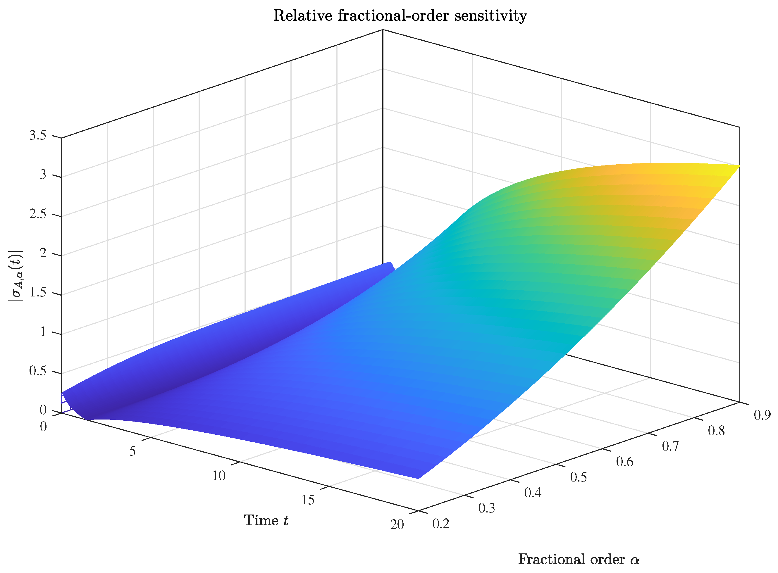
while maintaining $\kappa$ fixed. The behavior of $|{\sigma }_{A,\alpha }\left(t\right)|$ can be interpreted through the large-time asymptotics of the state. From Equation (25),

$$A\left(t\right)\sim {\displaystyle \frac{k_{01}}{k_{10,f}}}{\displaystyle \frac{t^{1-\alpha }}{\Gamma (2-\alpha )}},t\to \infty .$$

Using

$$k_{10,f}=\kappa t_{*}^{-\alpha },$$

we obtain

$$A\left(t\right)\sim {\displaystyle \frac{k_{01}}{\kappa }}{\displaystyle \frac{t_{*}^{\alpha }{t}^{1-\alpha }}{\Gamma (2-\alpha )}},t\to \infty .$$

Therefore,

$${\displaystyle \frac{1}{A\left(t\right)}}{\displaystyle \frac{\partial A\left(t\right)}{\partial \alpha }}\sim -ln\left({\displaystyle \frac{t}{t_{*}}}\right)+\psi (2-\alpha ),t\to \infty ,$$

and hence

$${\sigma }_{A,\alpha }\left(t\right)\sim \alpha \left[-ln\left({\displaystyle \frac{t}{t_{*}}}\right)+\psi (2-\alpha )\right],t\to \infty .$$

(80)

In particular,

$$|{\sigma }_{A,\alpha }\left(t\right)|=O(lnt),t\to \infty .$$

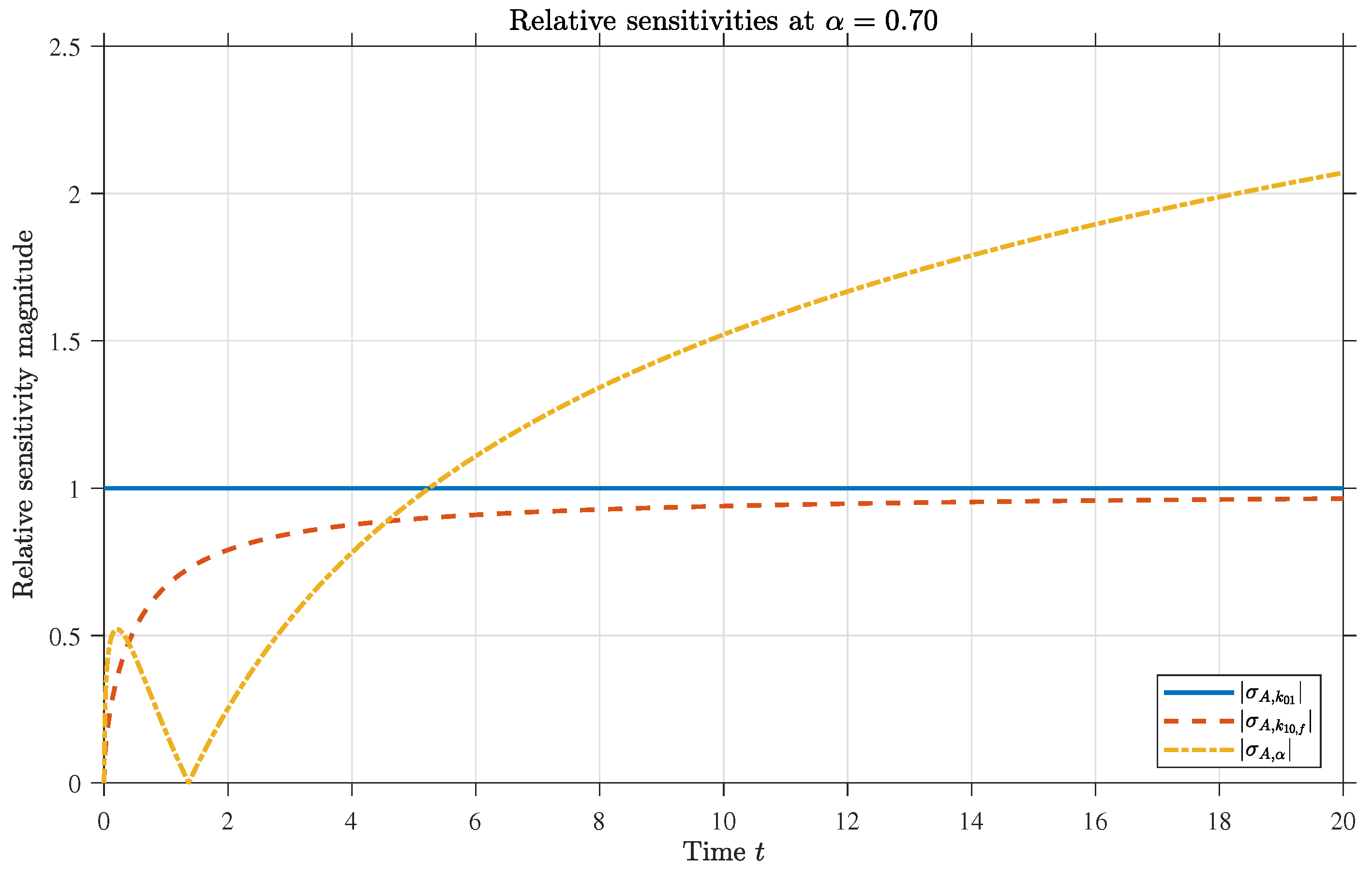
Thus the relative sensitivity with respect to the fractional order varies logarithmically at large times. Its dependence on t and $\alpha$ is illustrated in Figure 3.

We next compare the fractional-order sensitivity with those associated with the classical parameters at the nominal value $\alpha =0.70$. From Equation (73), ${\sigma }_{A,k_{01}}\left(t\right)=1.$ Moreover, the large-time asymptotics of the state yield

$${\sigma }_{A,k_{10,f}}\left(t\right)⟶-1,t\to \infty ,$$

and hence

$$|{\sigma }_{A,k_{10,f}}\left(t\right)|⟶1.$$

The negative sign reflects the inverse dependence of the state on the fractional elimination coefficient. In contrast, Equation (80) gives

$${\sigma }_{A,\alpha }\left(t\right)=-\alpha ln\left({\displaystyle \frac{t}{t_{*}}}\right)+O\left(1\right),t\to \infty .$$

Thus the three normalized sensitivities exhibit distinct asymptotic regimes: ${\sigma }_{A,k_{01}}$ is constant, ${\sigma }_{A,k_{10,f}}$ is asymptotically constant, whereas ${\sigma }_{A,\alpha }$ varies logarithmically at large times. The corresponding numerical comparison is displayed in Figure 4.

6. Discussion and Conclusions

The analysis developed in this work shows that flux–fractional compartment models and their associated sensitivity systems can be treated within a unified Sobolev–Volterra framework. The use of $W^{1,p}(0,T;H)$ is particularly natural, since both the Caputo memory term and the logarithmically weighted term arising from differentiation with respect to the fractional order are well defined as $L^p$-valued Volterra operators.

A central feature of the approach is the reduction in the problem to a Volterra equation for the velocity together with the use of an equivalent Bielecki norm. This makes it possible to obtain existence and uniqueness on arbitrary finite time intervals without imposing a smallness condition on the time horizon. The same formulation also provides a convenient basis for studying the dependence of the solution on the model parameters.

The differentiability result is important for the interpretation of the sensitivity equations. The classical parameter sensitivities and the fractional-order sensitivity are not merely formal auxiliary variables, but coincide with the corresponding derivatives of the parameter-to-solution map in $W^{1,p}$. In the fractional-order case, the introduction of the reference time $t_{*}$ provides a dimensionally consistent interpretation of differentiation with respect to $\alpha$ and leads naturally to the logarithmically weighted Caputo operator.

The one-compartment example illustrates several consequences of the general theory. In particular, the normalized sensitivities with respect to the input rate, the fractional elimination coefficient, and the fractional order exhibit qualitatively different long-time behavior. The input-rate sensitivity remains constant, the elimination sensitivity approaches a finite limit, whereas the fractional-order sensitivity retains a logarithmic dependence on time. This distinction reflects the different ways in which the corresponding parameters enter the flux–fractional dynamics.

The present results are restricted to linear flux–fractional systems. Nonlinear pharmacokinetic models would require additional assumptions on the nonlinear terms. Local well-posedness and differentiability may be expected under suitable local Lipschitz and smoothness conditions, whereas global results would generally require further growth, dissipativity, or a priori boundedness assumptions. Extending the present Sobolev–Volterra approach to such nonlinear systems provides a natural direction for future work.

References

1. Metzler, R.; Klafter, J. The Random Walk’s Guide to Anomalous Diffusion: A Fractional Dynamics Approach. Phys. Rep. 2000, 339, 1–77. [Google Scholar] [CrossRef] [Scilit]
2. Magin, R.L. Fractional Calculus in Bioengineering. Crit. Rev. Biomed. Eng. 2004, 32, 1–104. [Google Scholar] [CrossRef] [Scilit] [PubMed]
3. Podlubny, I. Fractional Differential Equations; An introduction to fractional derivatives, fractional differential equations, to methods of their solution and some of their applications; Mathematics in Science and Engineering; Academic Press, Inc.: San Diego, CA, USA, 1999; Volume 198. [Google Scholar]
4. Sopasakis, P.; Sarimveis, H.; Macheras, P.; Dokoumetzidis, A. Fractional calculus in pharmacokinetics. J. Pharmacokinet. Pharmacodyn. 2018, 45, 107–125. [Google Scholar] [CrossRef] [Scilit] [PubMed]
5. Dokoumetzidis, A.; Magin, R.; Macheras, P. Fractional Kinetics in Multi-Compartmental Systems. J. Pharmacokinet. Pharmacodyn. 2010, 37, 507–524. [Google Scholar] [CrossRef] [Scilit] [PubMed]
6. Dokoumetzidis, A.; Magin, R.; Macheras, P. A Commentary on Fractionalization of Multi-Compartmental Models. J. Pharmacokinet. Pharmacodyn. 2010, 37, 203–207. [Google Scholar] [CrossRef] [Scilit] [PubMed]
7. Angstmann, C.N.; Erickson, A.M.; Henry, B.I.; McGann, A.V.; Murray, J.M.; Nichols, J.A. Fractional Order Compartment Models. SIAM J. Appl. Math. 2017, 77, 430–446. [Google Scholar] [CrossRef] [Scilit]
8. Angstmann, C.N.; Henry, B.I.; Jacobs, B.A.; McGann, A.V. An Explicit Numerical Scheme for Solving Fractional Order Compartment Models from the Master Equations of a Stochastic Process. Commun. Nonlinear Sci. Numer. Simul. 2019, 68, 188–202. [Google Scholar] [CrossRef] [Scilit]
9. Qiao, Y.; Xu, H.; Qi, H. Numerical Simulation of a Two-Compartmental Fractional Model in Pharmacokinetics and Parameters Estimation. Math. Methods Appl. Sci. 2021, 44, 11526–11536. [Google Scholar] [CrossRef] [Scilit]
10. Mtshali, S.; Jacobs, B.A. On the Validation of a Fractional Order Model for Pharmacokinetics Using Clinical Data. Fractal Fract. 2023, 7, 84. [Google Scholar] [CrossRef] [Scilit]
11. Xu, Z.; Angstmann, C.N.; Han, D.; Henry, B.I.; Burney, S.J.M.; Jacobs, B.A. An Exact Stochastic Simulation Method for Fractional Order Compartment Models. SIAM J. Appl. Math. 2024, 84, 2132–2151. [Google Scholar] [CrossRef] [Scilit]
12. Li, C.; Qian, D.; Chen, Y. On Riemann–Liouville and Caputo Derivatives. Discret. Dyn. Nat. Soc. 2011, 562494. [Google Scholar] [CrossRef] [Scilit]
13. Miller, K.S.; Ross, B. An Introduction to the Fractional Calculus and Fractional Differential Equations; A Wiley-Interscience Publication; John Wiley & Sons, Inc.: New York, NY, USA, 1993; pp. xvi+366. [Google Scholar]
14. Bachar, M.; Desch, W.; Mardiyana. A Class of Semigroups Regularized in Space and Time. J. Math. Anal. Appl. 2006, 314, 558–578. [Google Scholar] [CrossRef] [Scilit]
15. Al-Gwaiz, M.A. Sturm-Liouville Theory and Its Applications, 2nd ed.; Springer Undergraduate Mathematics Series; Springer: London, UK, 2026; pp. xvi+269. [Google Scholar] [CrossRef] [Scilit]
16. Kilbas, A.A.; Srivastava, H.M.; Trujillo, J.J. Theory and Applications of Fractional Differential Equations; North-Holland Mathematics Studies; Elsevier Science B.V.: Amsterdam, The Netherlands, 2006; Volume 204, pp. xvi+523. [Google Scholar]
Figure 1. Solution A ( t , α ) = k 01 t E α , 2 ( k 10 , f t α ) of the one-compartment model with constant input, shown as a surface in ( t , α ) for 0 < α 1 . The red curves correspond to selected values of α and illustrate the approximately linear growth of A ( t ) for small t and the sublinear long-time growth A ( t ) ( k 01 / k 10 , f ) t 1 α / Γ ( 2 α ) for 0 < α < 1 .
Mathematics 14 03301 g001
Figure 2. Fractional flux in the one-compartment model with constant input. The surface shows the mapping ( t , α ) D 0 + 1 α C A ( t ) = k 01 t α E α , 1 + α ( k 10 , f t α ) for 0 < α 1 , with k 01 = 1 and k 10 , f = 1 . The horizontal plane at height k 01 / k 10 , f (grey) marks the asymptotic flux level lim t D 0 + 1 α C A ( t ) = k 01 / k 10 , f , while the red curves correspond to selected values of α and illustrate how the fractional flux approaches this limit for each order α .
Mathematics 14 03301 g002
Figure 3. Three-dimensional representation of the relative fractional-order sensitivity magnitude | σ A , α ( t ) | as a function of t and α for 0.2 α 0.9 .
Mathematics 14 03301 g003
Figure 4. Comparison of the relative sensitivity magnitudes | σ A , k 01 ( t ) | , | σ A , k 10 , f ( t ) | , and | σ A , α ( t ) | for α = 0.70 .
Mathematics 14 03301 g004
Disclaimer/Publisher’s Note: The statements, opinions and data contained in all publications are solely those of the individual author(s) and contributor(s) and not of MDPI and/or the editor(s). MDPI and/or the editor(s) disclaim responsibility for any injury to people or property resulting from any ideas, methods, instructions or products referred to in the content.