Dynamic Pressure Response and Wave Resistance in Forced Korteweg–DeVries Systems

Abstract

Weakly nonlinear free-surface flows past disturbances are traditionally modeled using the forced Korteweg–de Vries (fKdV) equation with a prescribed instantaneous pressure field. However, physical wake responses possess finite relaxation times and advection scales that diagnostic algebraic closures fail to capture. This paper introduces a novel coupled system in which the surface pressure is a dynamical field governed by an advection–reaction–diffusion equation driven by band-limited curvature. Using linear spectral theory and numerical validation, we derive a phase-speed criterion demonstrating that energy transfer is determined by the comparison between the pressure drift speed and the surface phase speed. A sharp stability theorem proves that, to leading order in the coupling strength and for a non-negative even response transfer function whose drift speed exceeds the Froude detuning, the system is spectrally stable if and only if the response is band-limited below a critical wavenumber $k_c$. Furthermore, an exact energy identity establishes that passivity and linear stability are equivalent. Finally, we demonstrate resonance steering: while coupling typically increases the wave resistance for monotone spectra, tuning the response to a spectral zero of a multi-lobe footprint reduces the drag significantly relative to its classical value. This result identifies an explicit performance–strongness trade-off, providing a mathematically strong structure for wave drag minimization through dynamic pressure control.

1. Introduction

Two-dimensional free-surface flow past a stern, a submerged obstacle or an applied pressure patch is one of the oldest and most-studied problems in hydrodynamics, and it remains active because of its direct bearing on wave drag. The fully nonlinear potential-flow formulation for a semi-infinite curved plate detaching into a free surface was solved by Vanden-Broeck [1], who showed that, for a given plate shape and Froude number, there is a one-parameter family of solutions indexed by a constant applied pressure. Binder [2] extended the analysis to a wider class of stern geometries, and Ogilat et al. [3] posed the design problem explicitly as minimization of wave drag over plate shape and pressure level. The linear finite-depth theory was developed by McCue and Stump [4] and McCue and Forbes [5], while Farrow and Tuck [6] treated more general stern shapes by boundary-integral methods, and Binder, Vanden-Broeck and Dias [7] clarified the correct numerical and analytical imposition of the radiation condition in such semi-infinite domains, a question revisited from the exponential-asymptotics side by Kataoka and Akylas [8].

Running parallel to the fully nonlinear theory is the weakly nonlinear long-wave reduction. For a Froude number near unity and small forcing, the free surface obeys a forced Korteweg–de Vries (fKdV) equation in which the forcing may represent bottom topography, an applied surface pressure, or a moving hull [9,10]. The fKdV structure has proved remarkably durable: Grimshaw and Maleewong analyzed transcritical flow over one and two obstacles and over holes [11,12], Binder [13] cataloged the stationary solution classes in the weakly nonlinear phase plane, Binder et al. [14] and Michalski et al. [15] established how obstacle length and height control the downstream response and identified discrete geometries for which no downstream waves are radiated, and Robbins et al. [16] developed an inverse method that constructs the forcing required to realize a prescribed free surface. Most recently, Keeler, Binder and Blyth [17] demonstrated computationally that suitably shaped pressure distributions can eliminate the nonlinear Kelvin wake over a range of Froude numbers, sharpening a line of inquiry that goes back to Tuck and Lazauskas [18]. In a complementary direction, the response of fKdV-type systems to external forcing that is periodic, moving, damped or stochastic has been mapped out in detail [19,20,21,22,23,24,25].

What all of this work shares is a structural assumption: the pressure acting on the free surface is prescribed. It is a constant [1,2,3], a fixed function of x [12,17], or, in the closely related wind-wave literature, an instantaneous algebraic functional of the surface itself. Zdyrski and Feddersen [26] take a Jeffreys-type pressure proportional to the surface slope [27], and Maleewong and Grimshaw [28,29] take forcing terms representing the Miles critical-layer mechanism [30]; in both cases the pressure is determined diagnostically pointwise from $\eta$ and its derivatives, and the outcome is a KdV–Burgers equation. A diagnostic closure retains no history; the pressure at a point is determined by the surface at that same point and instant.

Near a real stern this is precisely what fails. The pressure field of a separated or recirculating wake is not a diagnostic function of the local surface shape; it is advected, it relaxes on a finite time scale, it diffuses, and it responds only over a finite band of spatial scales because no physical pressure field, and no physical actuator, can respond to curvature variation on arbitrarily fine scales. The question this paper asks is therefore structural rather than cosmetic: what changes when the applied pressure is promoted from a prescribed function to a dynamical field with its own evolution equation? The answer turns out to be governed by a single clean mechanism. Giving the pressure a finite response time and drift speed introduces a phase lag between the surface and the pressure it generates, and the sign of the work done by that lagged pressure is decided by comparing the drift speed with the phase speed of the surface wave. This is the same structure as Miles’ critical-layer criterion, but it arises here without any shear flow: relaxation alone supplies the phase lag. That single observation organizes everything that follows: the stability criterion, the bandwidth constraint, the sign of the wave resistance, and the design result.

Contributions

We state each contribution at the level of rigor it can carry.

• A new coupled model (Section 2). We derive, with a consistent scaling ledger, a system coupling the fKdV equation to an advection–reaction–diffusion equation for the surface pressure driven by band-limited surface curvature (Equations (2)–(5)). We show that it contains the classical prescribed-pressure fKdV model ($\beta =0$) and a Jeffreys-type diagnostic closure ($\gamma \to \infty$) as limits and that the instantaneous limit is energetically neutral.
• A phase-speed criterion (Theorem 1). The exact $O\left(\beta \right)$ growth rate is

  $$\sigma \left(k\right)={\displaystyle \frac{\beta k^4\widehat{E}\left(k\right)\left[c_p\left(k\right)-\alpha \right]}{{2\left|D\left(k\right)\right|}^2}},c_p\left(k\right)=\Delta +{\displaystyle \frac{k^2}{6}}.$$
  Energy flows to the wave when the wave’s phase speed exceeds the drift speed of the pressure pattern and away from it otherwise.
• A sharp bandwidth theorem (Theorem 2). Spectral stability at every wavenumber holds if and only if $\mathrm{supp}\widehat{E}\subseteq [-k_c,k_c]$ with $k_c=\sqrt{6(\alpha -\Delta )}$. We also correct a natural but false expectation: without band-limiting, the growth rate does not blow up; it saturates at $3\beta$ (Proposition 2), so the unregularized system is uniformly unstable but well posed.
• Passivity equals stability (Theorem 3). An exact identity gives $R_g+R_d=0$, valid even with the nonlinear term retained, and a closed-form quadrature yields $\mathrm{sgn}{R}_g=\mathrm{sgn}\left(\alpha \beta \right)=-\mathrm{sgn}\sigma \left(k_0\right)$.
• A no-go result and a constructive escape (Section 7). Stable coupling always redshifts the resonance; for footprints with monotone spectrum this necessarily increases the wave resistance (up to a factor of $5.07$ in our computations). For footprints with a spectral zero the shift can be steered onto that zero, reducing the resistance to $13.1\%$ of its classical value while remaining stable, with an explicit trade-off law between the achievable reduction and the stability margin.
• Threefold validation (Section 8). Closed-form residues, spectral inversion and time marching from rest agree to under $1\%$ on amplitude, decay rate and wavenumber; measured modal growth rates reproduce the eigenvalue prediction to four significant figures; and the linear reduction is recovered from the full nonlinear system at rate $O\left(a\right)$.

Table 1. Treatment of the surface pressure in previous model classes and in the present work. Rows 1 and 4 are recovered from row 5 as the limits $\beta =0$ and $\gamma \to \infty$ (Proposition 1). “Energy exchange” means net work done by the applied pressure on the free surface at linear order.

Model Class	Pressure Treatment	Control Mechanism	Energy Exchange	Stability Constraint
Fully nonlinear prescribed pressure [1,2,3]	Constant applied pressure	Plate shape and pressure level	None (conservative)	Not applicable
Weakly nonlinear fKdV [9,10,12,13]	Prescribed function of position	Obstacle or footprint geometry	None	Not applicable
Wave-free and inverse designs [15,16,17,18]	Prescribed, optimized	Geometry chosen so that ${\widehat{p}}_0$ vanishes at the radiated wavenumber at a single operating point	None	Not applicable
Diagnostic closures, Jeffreys-type and Miles-type [26,27,28,30]	Instantaneous algebraic functional of $\eta$	None; the pressure is slaved to the surface	Through odd-derivative terms (KdV–Burgers)	Sign of the closure coefficient
Present work	Dynamical field, Equation (5)	Coupling strength $\beta$ and drift speed $\alpha$, tunable across operating points	Yes; sign fixed by $c_p\left(k\right)-\alpha$	$\mathrm{supp}\widehat{E}\subseteq [-k_c,k_c]$

places the model in relation to the four classes of previous work surveyed above, classified by the treatment of the surface pressure. The essential point is that the first and fourth rows are not merely analogous to the present model but are contained in it as the limits $\beta =0$ and $\gamma \to \infty$, respectively. The distinction that matters for drag reduction is in the third column: wave-free and inverse designs place a spectral zero of the forcing at the radiated wavenumber by choosing the geometry so that the cancellation is fixed at one operating point, whereas here the resonance itself is moved and the coupling strength can track a zero as the Froude number changes.

This is a two-dimensional weakly nonlinear study with a phenomenological pressure closure. Section 9 states precisely what would be needed before the design conclusions could be taken to a real hull.

2. Formulation

We take the standard configuration of [1,2,4]: steady two-dimensional flow of an inviscid incompressible fluid that is irrotational in a channel of undisturbed depth H, with a uniform stream of speed U in the $+x$ direction and a free surface carrying an applied pressure. Lengths are scaled by H, speeds by $\sqrt{gH}$ and pressures by $\rho gH$ so that the Froude number is $F=U/\sqrt{gH}$.

Writing the Boussinesq system [31] for the depth-averaged velocity u and elevation $\eta$ with an applied surface pressure p,

$${\eta }_t+{\left[(1+\eta )u\right]}_x=0,u_t+u{u}_x+{\eta }_x+p_x=\frac{1}{3}{u}_{xxt},$$

(1)

and following the standard near-critical reduction, we set $u=U-\eta +\epsilon w$, which selects the slow (left-running) Riemann invariant, the one whose speed $U-1$ is small when $F\approx 1$. Eliminating w at leading order gives

$${\eta }_{\tau }+\Delta {\eta }_X-\frac{3}{2}\eta {\eta }_X-\frac{1}{6}{\eta }_{XXX}=\frac{1}{2}{\left(p_0+P\right)}_X,$$

(2)

where $\Delta =U-1$ is the Froude detuning, $p_0$ is the static footprint associated with the stern geometry, and P is the dynamic pressure introduced below. Equation (2) is exactly the canonical fKdV equation in the convention of [12,20], including the coefficient $\frac{3}{2}$ of the nonlinear term and the sign of the dispersive term.

Remark 1 (Orientation and the sign of Δ).

The linear dispersion relation of (2) is $\omega =\Delta k+k^3/6$, so the phase and group speeds in the stern frame are

$$c_p\left(k\right)=\Delta +{\displaystyle \frac{k^2}{6}},c_g\left(k\right)=\Delta +{\displaystyle \frac{k^2}{2}}.$$

(3)

A stationary lee wave requires $c_p\left(k_0\right)=0$, i.e.,

$$k_0=\sqrt{-6\Delta },\Delta <0\left(\mathit{subcritical}\right),$$

(4)

and then $c_g\left(k_0\right)=-2\Delta >0$: the radiated energy travels in the $+X$ direction, so the wavetrain lies downstream of the forcing as it must. Supercritical flow, $\Delta >0$, gives no real $k_0$ and no wavetrain. All the results below are for $\Delta <0$. This bookkeeping is not pedantry: reversing either the dispersive or the forcing sign flips the direction of radiation and with it the sign of every energy-transfer statement in Section 3 and Section 5.

We now let the surface pressure carry its own dynamics. The physical ingredients are: drift of the pressure pattern relative to the stern at speed $\alpha$; relaxation towards equilibrium at rate $\gamma$; generation by surface curvature at rate $\beta$; and diffusive smoothing at rate $\delta$. Crucially, the curvature that drives the response is band-limited: we write

$$P_{\tau }+\alpha P_X=\beta {\mathcal{K}}_b\left[\eta \right]-\gamma P+\delta P_{XX},$$

(5)

where ${\mathcal{K}}_b$ is the mollified curvature operator with Fourier symbol

$$\widehat{{\mathcal{K}}_b}\left(k\right)=-k^2\widehat{E}\left(k\right),\widehat{E}\mathrm{even},\widehat{E}\ge 0,\widehat{E}\left(0\right)=1.$$

(6)

The response transfer function $\widehat{E}$ encodes the finite spatial bandwidth of the pressure response. Section 3 shows that its support is not a technical convenience but the object on which well-posedness turns. For all the computations we take the smooth compactly supported Friedrichs bump

$$\widehat{E}\left(k\right)=\left\{\begin{array}{cc}\exp \left[1-{\left(1-{(k/k_b)}^2\right)}^{-1}\right],\hfill & \left|k\right|<k_b,\hfill \\ 0,\hfill & \left|k\right|\ge k_b,\hfill \end{array}\right.$$

(7)

which is $C^{\infty }$, has $\widehat{E}\left(0\right)=1$, and is real-analytic on the open interval $(-k_b,k_b)$, enough for the local continuation used in Section 4. Gaussian and Butterworth alternatives are compared in Section 3.

The five response parameters and the speeds used throughout are collected in

Table 2. Parameters of the response Equation (5) and derived quantities. All variables are non-dimensional: lengths are scaled by the depth H, speeds by $\sqrt{gH}$ and pressures by $\rho gH$, so the parameters themselves are dimensionless numbers. The third column gives the dimensional character of each in the reduced stern-frame variables of (2) and (5); the fourth gives the order forced by the scaling ledger of Table 3.

Symbol	Meaning	Character	Order
$\Delta =U-1$	Froude detuning; $\Delta <0$ is subcritical and is required for a stationary lee wave	Speed	$ϵ$
$\alpha$	Drift speed of the pressure pattern relative to the stern (advection coefficient)	Speed	$ϵ$
$\beta$	Rate at which band-limited surface curvature generates pressure (coupling strength)	Rate	${ϵ}^{3/2}$
$\gamma$	Relaxation rate of the pressure towards equilibrium; $1/\gamma$ is the response time	Rate	${ϵ}^{3/2}$
$\delta$	Diffusivity smoothing the pressure field	Diffusivity	${ϵ}^{1/2}$
$k_b$	Cut-off wavenumber of $\widehat{E}$ (response bandwidth); $2\pi /k_b$ is the shortest surface feature to which the pressure responds	Inverse length	$O\left(1\right)$
$c_p\left(k\right)=\Delta +k^2/6$	Surface phase speed in the stern frame	Speed	—
$c_g\left(k\right)=\Delta +k^2/2$	Group speed; sets the direction of radiation	Speed	—
$k_0=\sqrt{-6\Delta }$	Stationary lee wavenumber, $c_p\left(k_0\right)=0$	Inverse length	—
$k_c=\sqrt{6(\alpha -\Delta )}$	Critical wavenumber of Theorem 2 at which $c_p\left(k_c\right)=\alpha$	Inverse length	—

. Two distinctions there are worth stating explicitly because they are easily conflated. First, $1/\gamma$ and $k_b$ are both “response” scales but are not the same kind of object: $1/\gamma$ is the time the pressure takes to relax towards equilibrium, whereas $k_b$ is the finest spatial scale to which it responds at all. Proposition 1 turns on the first, Theorem 2 on the second. Second, the drift speed $\alpha$ is a property of the pressure field, whereas the phase speed $c_p\left(k\right)$ and group speed $c_g\left(k\right)$ are properties of the surface wave; the whole of Section 3 rests on comparing the first with the second. We therefore use “drift speed” for $\alpha$, “phase speed” for $c_p$ and “group speed” for $c_g$ exclusively and refer to $1/\gamma$ and $k_b$ as the response time and the response bandwidth rather than as a response speed.

Equation (5) is only meaningful if it sits at the same asymptotic order as (2). With the standard transcritical scalings $\eta =O\left(ϵ\right)$, ${\partial }_X=O\left({ϵ}^{1/2}\right)$, ${\partial }_{\tau }=O\left({ϵ}^{3/2}\right)$, and $\Delta =O\left(ϵ\right)$, every term of (2) is $O\left({ϵ}^{5/2}\right)$ provided $p_0,P=O\left({ϵ}^2\right)$. Requiring every term of (5) to be $O\left({ϵ}^{7/2}\right)$ then fixes the response parameters uniquely, as set out in

Table 3. Orders in the small parameter $ϵ$. The right-hand column gives the order of each term of (5); all are $O\left({ϵ}^{7/2}\right)$, so the pressure equation balances at a single order.

Quantity	Order	Term of (5)	Order
$\eta ,{\partial }_X,{\partial }_{\tau },\Delta$	$ϵ,{ϵ}^{1/2},{ϵ}^{3/2},ϵ$	$P_{\tau }$	${ϵ}^{7/2}$
$p_0,P$	${ϵ}^2$	$\alpha P_X$	$ϵ·{ϵ}^{5/2}$
$\alpha$ (drift speed)	$ϵ$	$\beta {\mathcal{K}}_b\left[\eta \right]$	${ϵ}^{3/2}·{ϵ}^2$
$\gamma$ (relaxation rate)	${ϵ}^{3/2}$	$\gamma P$	${ϵ}^{3/2}·{ϵ}^2$
$\delta$ (diffusivity)	${ϵ}^{1/2}$	$\delta P_{XX}$	${ϵ}^{1/2}·{ϵ}^3$
$\beta$ (coupling)	${ϵ}^{3/2}$

.

Remark 2 (What the scaling ledger forces).

Table 3 carries real physical content and should not be skipped. It requires $\alpha =O\left(ϵ\right)$: the pressure field drifts slowly relative to the stern. A field advected passively with the mean stream would have drift speed $O\left(1\right)$, hence $O\left({ϵ}^{-1}\right)$ in reduced variables, and is therefore inadmissible at this order: it degenerates into the diagnostic limit of Proposition 1. The model (2)–(5) is thus a slow-response closure governed by persistent relaxation dynamics, which is appropriate for a wake pressure field quasi-locked to the stern or an actuated surface-pressure system but not for a passive scalar swept downstream by the free stream. We regard this as a feature rather than a restriction: it identifies precisely the regime in which pressure dynamics can matter at leading order.

For a real hull this is a statement of scope rather than a technicality, and it is worth spelling out. The admissible field is one that stays quasi-locked to the stern: a recirculating or separated near-stern region whose pressure pattern moves only slowly relative to the hull or an actuated surface-pressure system whose actuators are fixed to the hull and whose drift speed is therefore a design choice. A pressure disturbance shed from the stern and swept downstream with the mean stream is excluded, and, by Proposition 1, such a field would, in any case, do no net work on the surface and could not produce the energy transfer studied here. The results of Section 3 and Section 7 should accordingly be read as applying to the near-stern region and to active pressure control, not to the far-field advected wake. This also tells an experimentalist where to look: the quantity to be measured when calibrating α is the translation speed of the near-stern pressure pattern in the hull frame, which the model requires to be small compared with the stream speed.

Setting $\beta =0$ returns the classical fKdV equation forced by the prescribed footprint $p_0$ alone, i.e., the weakly nonlinear limit of the constant- and prescribed-pressure theories [1,2,3,12].

Proposition 1 (Instantaneous limit is energetically neutral).

Let $\gamma \to \infty$ with $b=\beta /\gamma$ fixed. Then $\widehat{P}\to -b{k}^2\widehat{E}\widehat{\eta }$ uniformly on compact k-sets so that $P\to b{\mathcal{K}}_b\left[\eta \right]$ and (2) becomes ${\eta }_{\tau }+\Delta {\eta }_X-\frac{3}{2}\eta {\eta }_X-\frac{1}{6}{\eta }_{XXX}=\frac{1}{2}{p}_{0X}+\frac{b}{2}{\mathcal{K}}_b{\left[\eta \right]}_X$. The added operator has a purely imaginary Fourier symbol; it modifies the dispersion relation (acting like a band-limited surface tension) and does no net work on the surface. The first correction in ${\gamma }^{-1}$ produces an odd-derivative Jeffreys-type term of the kind used in [26,28], and it is this term that carries the energy exchange.

Proof. 

From (5) in Fourier variables, $\widehat{P}=-\beta k^2\widehat{E}\widehat{\eta }/(\gamma +i\alpha k+\delta k^2)$; the limit is immediate. The symbol of $\frac{b}{2}{\partial }_X{\mathcal{K}}_b$ is $\frac{b}{2}\left(ik\right)(-k^2\widehat{E})=-\frac{i}{2}b{k}^3\widehat{E}$, purely imaginary, and hence contributes nothing to $\frac{d}{d\tau }\int {\eta }^2$. Expanding ${(\gamma +i\alpha k+\delta k^2)}^{-1}={\gamma }^{-1}[1-(i\alpha k+\delta k^2)/\gamma +O\left({\gamma }^{-2}\right)]$ produces a real contribution at $O\left({\gamma }^{-2}\right)$ proportional to $\alpha$, which is the dissipative (or anti-dissipative) part.  □

Proposition 1 is the pivot of the whole paper: instantaneous curvature coupling cannot transfer energy; every stability and drag result below originates in the phase lag created by finite $\gamma$ and $\alpha$.

We state the status of (5) plainly since everything that follows is conditional on it. It is a phenomenological closure, not a reduction of a boundary-layer or wake model. Its claim to attention is that of a minimal model. Each term corresponds to one identifiable feature of a wake pressure field: advective drift, relaxation, generation by curvature, diffusion, and a finite response bandwidth expressing that no physical pressure field and no physical actuator responds to curvature on arbitrarily fine scales. Table 3 shows that requiring these terms to balance at the order of the fKdV reduction fixes all five parameters uniquely rather than leaving them free. It contains the classical prescribed-pressure model and the Jeffreys-type diagnostic closure as the limits $\beta =0$ and $\gamma \to \infty$, so it is a strict generalization of both. It has not been calibrated against separated-flow measurements or Reynolds-averaged computations and we make no claim that it has; what such a calibration would have to determine, and what would have to be checked in the process, is set out in Section 9.

3. Linear Spectral Theory

Linearizing (2)–(5) about $\eta =P=0$, discarding the forcing, and transforming in X (${\partial }_X\mapsto ik$) gives $\frac{d}{d\tau }{(\widehat{\eta },\widehat{P})}^{\top }=M\left(k\right){(\widehat{\eta },\widehat{P})}^{\top }$ with

$$M\left(k\right)=\left(\begin{array}{cc}-ik{c}_p\left(k\right)& {\displaystyle \frac{i}{2}}k\\ -\beta k^2\widehat{E}\left(k\right)& -(\gamma +\delta k^2)-i\alpha k\end{array}\right)$$

(8)

with $c_p\left(k\right)$ as in (3). Write $D\left(k\right):=M_{11}-M_{22}=D_R+i{D}_I$ with

$$D_R=\gamma +\delta k^2>0,D_I=k\left(\alpha -c_p\left(k\right)\right).$$

(9)

Because $M_{21}$ is the only $\beta$-dependent entry, the eigenvalues are available in closed form,

$${\lambda }_{\pm }\left(k\right)={\displaystyle \frac{1}{2}}\left[\mathrm{tr}M\pm \sqrt{D^2+2i\beta k^3\widehat{E}}\right],$$

(10)

with the branch fixed by continuity from $\beta =0$.

Theorem 1 (Phase-speed criterion).

Let $\sigma \left(k\right):=\max \{\mathrm{Re}{\lambda }_{+}\left(k\right),\mathrm{Re}{\lambda }_{-}\left(k\right)\}$. Then

$$\sigma \left(k\right)={\displaystyle \frac{\beta k^4\widehat{E}\left(k\right)\left[c_p\left(k\right)-\alpha \right]}{{2\left|D\left(k\right)\right|}^2}}+O\left({\beta }^2\right)$$

(11)

uniformly on compact k-sets. In particular, for $\beta >0$ and $\widehat{E}\ge 0$, the sign of $\sigma \left(k\right)$ is the sign of $c_p\left(k\right)-\alpha$: the wave of wavenumber k is damped when the pressure pattern drifts faster than the wave’s phase speed and amplified when it drifts slower.

Proof. 

Since $M_{12}{M}_{21}=-\frac{i}{2}\beta k^3\widehat{E}$ is $O\left(\beta \right)$ while D is $\beta$-independent, expansion of (10) gives ${\lambda }_{+}=M_{11}+M_{12}{M}_{21}/D+O\left({\beta }^2\right)$. Since $\mathrm{Re}{M}_{11}=0$,

$$\mathrm{Re}{\displaystyle \frac{M_{12}{M}_{21}}{D}}=\mathrm{Re}{\displaystyle \frac{-\frac{i}{2}\beta k^3\widehat{E}(D_R-i{D}_I)}{{\left|D\right|}^2}}=-{\displaystyle \frac{\beta k^3\widehat{E}{D}_I}{{2\left|D\right|}^2}},$$

and substituting $D_I=k[\alpha -c_p]$ from (9) gives (11). The remaining eigenvalue satisfies $\mathrm{Re}{\lambda }_{-}=-(\gamma +\delta k^2)-\mathrm{Re}{\lambda }_{+}<0$ for small $\beta$, so the maximum is attained by ${\lambda }_{+}$. Expression (11) is even in k as required by reality.  □

Remark 3 (Relation to Miles’ mechanism).

Equation (11) has the structure of a critical-layer criterion: the transfer changes sign where the forcing pattern and the wave are in phase-speed resonance, $c_p\left(k\right)=\alpha$. In Miles’ theory [30] the matching is between the wave and a sheared air flow; here there is no shear at all, and the phase lag is supplied entirely by the relaxation of the pressure field (Proposition 1). The two mechanisms are formally analogous but physically distinct.

Proposition 2 (Unregularized coupling: bounded growth, not ill-posedness).

Let $\widehat{E}\equiv 1$. Then $\sigma \left(k\right)\to 3\beta$ as $\left|k\right|\to \infty$, with $\sigma \left(k\right)=3\beta [1+(6(\alpha -\Delta )-36{\delta }^2)k^{-2}+O\left(k^{-4}\right)]$. Consequently ${\sup }_k\sigma \left(k\right)<\infty$: the semigroup satisfies $\parallel u\left(\tau \right)\parallel \le C{e}^{c\beta \tau }\parallel u\left(0\right)\parallel$ in the same norm, so the initial-value problem is well posed in the sense of Hadamard although uniformly unstable: every sufficiently short wave is amplified at essentially the same rate.

Proof. 

As $\left|k\right|\to \infty$, $D\sim -i{k}^3/6$ and $M_{12}{M}_{21}=-\frac{i}{2}\beta k^3$, so $M_{12}{M}_{21}/D\to 3\beta$; the correction follows from writing $D=-\frac{i{k}^3}{6}\left[1-6(\alpha -\Delta )k^{-2}+6i\delta k^{-1}+6i\gamma k^{-3}\right]$, whence $-\beta k^3{D}_I=\frac{\beta k^6}{6}\left[1-6(\alpha -\Delta )k^{-2}\right]$ and ${\left|D\right|}^2=\frac{k^6}{36}\left[1-\left(12(\alpha -\Delta )-36{\delta }^2\right)k^{-2}+O\left(k^{-4}\right)\right]$, and forming the quotient $\sigma =-\beta k^3{D}_I/{\left(2\right|D|}^2)$.  □

Proposition 2 corrects an intuition that is natural but wrong. Comparing the off-diagonal product $\beta k^3$ with the diagonal damping $\delta k^2$ suggests unbounded growth; the correct comparison for a $2\times 2$ matrix with separated diagonal entries is $M_{12}{M}_{21}$ against ${(M_{11}-M_{22})}^2\sim -k^6/36$, and that ratio tends to zero. The verification in

Table 4. Short-wave saturation of the growth rate for $\widehat{E}\equiv 1$ (Proposition 2). Entries are $\mathrm{Re}{\lambda }_{+}\left(k\right)$ computed from the exact quadratic (10); $\Delta =-0.15$, $\alpha =0.5$, $\gamma =1$, and $\delta =0.2$.

	$\mathit{k}=50$	$\mathit{k}=200$	$\mathit{k}=1000$	$\mathit{k}=5000$
$\beta =0.05$ ($3\beta =0.15$)	0.15014718	0.15000922	0.15000037	0.15000001
$\beta =0.20$ ($3\beta =0.60$)	0.60058780	0.60003689	0.60000148	0.60000006
$\beta =0.50$ ($3\beta =1.50$)	1.50146479	1.50009221	1.50000369	1.50000015

confirms saturation to six significant figures.

Theorem 2 (Sharp bandwidth criterion).

Let $\beta >0$, $\widehat{E}\ge 0$ even, and $\alpha >\Delta$ and set

$$k_c:=\sqrt{6(\alpha -\Delta )}.$$

(12)

Then, to $O\left(\beta \right)$, $\sigma \left(k\right)\le 0$ for every $k\in \mathbb{R}$ if and only if

$$\mathrm{supp}\widehat{E}\subseteq [-k_c,k_c].$$

(13)

Moreover the stationary lee wave $k_0=\sqrt{-6\Delta }$ lies strictly inside the admissible band if and only if $\alpha >0$, and, when $\widehat{E}$ does not vanish outside $[-k_c,k_c]$, ${\sup }_k\sigma \left(k\right)=3\beta {\sup }_{\left|k\right|>k_c}\widehat{E}\left(k\right)+O\left({\beta }^2\right)$.

Proof. 

By (11), $\sigma \left(k\right)\le 0$ iff $\widehat{E}\left(k\right)[c_p\left(k\right)-\alpha ]\le 0$. Since $c_p$ is increasing in $\left|k\right|$ with $c_p\left(0\right)=\Delta <\alpha$, we have $c_p\left(k\right)\le \alpha \iff k^2\le 6(\alpha -\Delta )$. Hence $\sigma \le 0$ everywhere iff $\widehat{E}$ vanishes wherever $\left|k\right|>k_c$. For the second claim, $k_0<k_c\iff -6\Delta <6(\alpha -\Delta )\iff \alpha >0$. The final estimate follows from Proposition 2 applied on $\left\{\right|k|>k_c\}$.  □

Remark 4 (Physical reading of the criterion).

The critical wavenumber is kinematic rather than technical. Since $c_p\left(k\right)=\Delta +k^2/6$ increases with $\left|k\right|$ from $c_p\left(0\right)=\Delta$, the equation $c_p\left(k\right)=\alpha$ has the unique positive root $k_c=\sqrt{6(\alpha -\Delta )}$ of (12). Thus $k_c$ is the wavenumber whose wave travels, in the stern frame, at exactly the drift speed of the pressure pattern.

The mechanism behind Theorem 1 then reads as follows. A pressure field with finite relaxation time cannot follow the surface instantaneously; it follows with a lag, and, because the pattern also drifts at its own speed, the sign of that lag depends on which of the two moves faster. For $\left|k\right|<k_c$ the wave is slower than the pattern, the pressure maximum ends up ahead of the surface elevation that generated it, and the lagged pressure does negative work: the wave is damped. For $\left|k\right|>k_c$ the wave outruns the pattern, the lag reverses, and the wave is amplified. Theorem 2 therefore states that the system is stable precisely when the pressure field is incapable of responding to any wave faster than itself.

In the actuated reading this is a bandwidth specification for the controller: an actuator that responds to surface features shorter than $2\pi /k_c$ injects energy into them, and the requirement $\mathrm{supp}\widehat{E}\subseteq [-k_c,k_c]$ is the instruction not to build one. Corollary 1 adds the complementary condition: the stationary lee wave lies inside the admissible band exactly when the pattern drifts downstream at all, $\alpha >0$, such that a stable design that nevertheless acts on the wave of interest exists if and only if the drift is in the direction of the stream.

Corollary 1 (Design window).

If $\alpha >0$ then the band $k_0<k_b\le k_c$ is nonempty, and any transfer function supported in $[-k_b,k_b]$ yields a spectrally stable system in which the coupling nevertheless acts on the stationary lee wave. All computations below use $\Delta =-0.15$ and $\alpha =0.5$, giving $k_0=0.9486833$, $k_c=1.9748418$, and the choice $k_b=1.6$.

Remark 5 (What “stable” means here).

For $\left|k\right|>k_b$ the transfer function vanishes, $M_{21}=0$, and the surface equation decouples: those modes are free dispersive waves with $\mathrm{Re}\lambda =0$. Spectral stability therefore means ${\sup }_k\sigma \left(k\right)=0$, attained on the conservative modes, with $\sigma \left(k\right)<0$ strictly on the response band. This is the best that can be asked of a system whose uncoupled limit is conservative.

Table 5. Sharpness of the bandwidth criterion. ${\max }_k\mathrm{Re}\lambda$ over $k\in [0,12]$ for $\beta =0.2$, $\Delta =-0.15$, $\alpha =0.5$, $\gamma =1$, and $\delta =0.2$ so that $k_c=1.9748418$. Entries below ${10}^{-14}$ are at round-off; recall that ${\sup }_k\sigma =0$ is the stable value.

${\mathit{k}}_{\mathit{b}}$	1.20	1.60	1.90	${\mathit{k}}_{\mathit{c}}$	2.05	2.20	2.60
${\max }_k\mathrm{Re}\lambda$	0	0	0	0	$1.52\times {10}^{-9}$	$7.99\times {10}^{-5}$	$9.82\times {10}^{-3}$
$\mathrm{argmax}k$	—	—	—	—	1.980	2.006	2.104
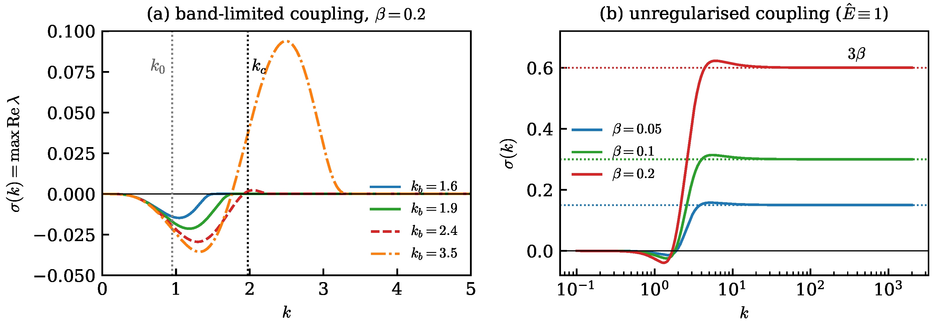
verdict	stable	stable	stable	stable	unstable	unstable	unstable

and

Table 6. Only compactly supported transfer functions give exact stability. $\beta =0.2$, $k_b=1.6$, and $k_c=1.9748418$; “estimate” is $3\beta {\sup }_{\left|k\right|>k_c}\widehat{E}$ from Theorem 2, accurate to $O\left({\beta }^2\right)$.

$\widehat{\mathit{E}}\left(\mathit{k}\right)$	${\sup }_{\mathit{k}}\mathit{\sigma }$	$\mathrm{argmax}\mathit{k}$	Estimate $3\mathit{\beta }{\sup }_{\left|\mathit{k}\right|>{\mathit{k}}_{\mathit{c}}}\widehat{\mathit{E}}$
Friedrichs bump (7)	$1.1\times {10}^{-13}$	—	0
Gaussian $e^{-{(k/k_b)}^2}$	$2.249\times {10}^{-2}$	2.509	$1.308\times {10}^{-1}$
Butterworth ${[1+{(k/k_b)}^8]}^{-1}$	$7.756\times {10}^{-3}$	2.315	$9.393\times {10}^{-2}$
Unregularized $\widehat{E}\equiv 1$	$6.228\times {10}^{-1}$	6.05	$6.000\times {10}^{-1}$

verify Theorem 2 numerically. The transition at $k_b=k_c$ is exact; the growth that appears for $k_b>k_c$ is at first extremely small because the Friedrichs bump vanishes to infinite order at its endpoints and grows rapidly thereafter.

4. Steady Radiating Solution

4.1. Modified Dispersion Function

Setting ${\partial }_{\tau }=0$ in the linearized system and eliminating $\widehat{P}$ gives, for $k\ne 0$,

$$\widehat{\eta }\left(k\right)={\displaystyle \frac{{\widehat{p}}_0\left(k\right)}{2\mathcal{D}\left(k\right)}},\mathcal{D}\left(k\right)=\Delta +{\displaystyle \frac{k^2}{6}}+{\displaystyle \frac{\beta k^2\widehat{E}\left(k\right)}{2\left(\gamma +i\alpha k+\delta k^2\right)}}.$$

(14)

The function $\mathcal{D}$ is the exact analogue, for the pressure-coupled problem, of the classical dispersion function $\Delta +k^2/6$, whose real zeros give the radiated wavenumber. Its real and imaginary parts on the real axis are

$${\mathcal{D}}_R=\Delta +{\displaystyle \frac{k^2}{6}}+{\displaystyle \frac{\beta k^2\widehat{E}(\gamma +\delta k^2)}{2Q}},{\mathcal{D}}_I=-{\displaystyle \frac{\alpha \beta k^3\widehat{E}}{2Q}},Q:={(\gamma +\delta k^2)}^2+{\alpha }^2{k}^2.$$

(15)

4.2. Radiation Condition

For $\beta =0$, $\mathcal{D}$ has real zeros at $\pm k_0$, and a radiation condition must be imposed. We use limiting absorption: add Rayleigh damping $-\mu \eta$ to (2) so that ${\mathcal{D}}_{\mu }=\mathcal{D}-i\mu /k$, whose zeros sit at $k=\pm k_0+3i\mu /k_0^2$ in the upper half plane. Closing the inversion contour upwards for $X>0$ then places the wavetrain downstream and leaves the upstream region wave-free, consistent with $c_g\left(k_0\right)>0$ (Remark 1). Evaluating the residues gives the closed form

$$\eta \left(X\right)⟶-A_0\sin \left(k_{0}X\right)(X>0),A_0={\displaystyle \frac{3{\widehat{p}}_0\left(k_0\right)}{k_0}},$$

(16)

which we use throughout as an exact benchmark.

For $\beta >0$ the situation is cleaner: by (15), ${\mathcal{D}}_I\ne 0$ for $k\ne 0$, so $\mathcal{D}$ has no real zeros and no regularization is needed. Writing $k_{\ast }=k_r+i\kappa$ for the zero of $\mathcal{D}$ continued from $k_0$, one finds $\kappa \approx -{\mathcal{D}}_I/{\mathcal{D}}_R^{\prime }>0$ when $\alpha \beta >0$, so $k_{\ast }$ again lies in the upper half plane and

$$\eta \left(X\right)\simeq A{e}^{-\kappa X}\cos \left(k_{r}X+\phi \right),A=\left|{\displaystyle \frac{{\widehat{p}}_0\left(k_{\ast }\right)}{{\mathcal{D}}^{\prime }\left(k_{\ast }\right)}}\right|(X>0).$$

(17)

We call A the emitted amplitude (the envelope extrapolated to $X=0^{+}$) and $\kappa$ the spatial attenuation rate. Both are unambiguous, unlike “the downstream amplitude”, which, for an attenuating wavetrain, depends on where it is measured. As $\beta \to 0$, ${\mathcal{D}}^{\prime }\left(k_0\right)=k_0/3$ and (17) reduces to (16).

Proposition 3 (Gaster relation).

Let $k_0^{\prime }$ denote the real zero of ${\mathcal{D}}_R$ (the shifted stationary wavenumber) and $c_g^{\mathrm{eff}}:=k_0^{\prime }{\mathcal{D}}_R^{\prime }\left(k_0^{\prime }\right)$ the corresponding group velocity. Then, in the weak-attenuation limit,

$$\kappa ={\displaystyle \frac{\left|\sigma \right(k_0^{\prime }\left)\right|}{c_g^{\mathrm{eff}}}}\left(1+O\left(\kappa \right)\right).$$

(18)

This is Gaster’s transformation [32] between temporal and spatial growth rates, here emerging unforced from the structure of $\mathcal{D}$; it is verified in

Table 7. Verification of the Gaster relation (18). Baseline parameters and single-lobe footprint. The deviation grows with $\beta$ because (18) is a weak-attenuation result.

$\mathit{\beta }$	${\mathit{k}}_0^{\prime }$	${\mathit{c}}_{\mathit{g}}^{\mathbf{eff}}$	$\left|\mathit{\sigma }\right({\mathit{k}}_0^{\prime }\left)\right|$	$\left|\mathit{\sigma }\right|/{\mathit{c}}_{\mathit{g}}^{\mathbf{eff}}$	$\mathit{\kappa }$ (Residue)
0.02	0.936512	0.292061	$1.42972\times {10}^{-3}$	$4.89530\times {10}^{-3}$	$4.88557\times {10}^{-3}$
0.05	0.917948	0.281436	$3.46521\times {10}^{-3}$	$1.23126\times {10}^{-2}$	$1.22574\times {10}^{-2}$
0.10	0.886516	0.266980	$6.52016\times {10}^{-3}$	$2.44219\times {10}^{-2}$	$2.42305\times {10}^{-2}$
0.20	0.824051	0.248491	$1.11970\times {10}^{-2}$	$4.50599\times {10}^{-2}$	$4.43361\times {10}^{-2}$
0.35	0.738523	0.238238	$1.48727\times {10}^{-2}$	$6.24279\times {10}^{-2}$	$5.99715\times {10}^{-2}$
0.50	0.667526	0.238082	$1.58891\times {10}^{-2}$	$6.67380\times {10}^{-2}$	$6.25850\times {10}^{-2}$

and provides a stringent consistency check linking Section 3 and Section 4.

5. Energy Budget, Wave Resistance and Passivity

Define the rates of working of the applied and induced pressures,

$$R_g:=-{\displaystyle \frac{1}{2}}{\int }_{\mathbb{R}}{\eta }_X{p}_{0}dX,R_d:=-{\displaystyle \frac{1}{2}}{\int }_{\mathbb{R}}{\eta }_{X}PdX.$$

(19)

$R_g$ is the long-wave wave-resistance functional: it is the force-based drag associated with the geometric footprint, and it reduces to the classical Havelock-type expression in the uncoupled limit (Proposition 4).

Theorem 3 (Exact absorption identity).

For any steady decaying solution of the full nonlinear system (2)–(5),

$$R_g+R_d=0.$$

(20)

Moreover, in the linear steady state,

$$R_g={\displaystyle \frac{\alpha \beta }{16\pi }}{\int }_{\mathbb{R}}{\displaystyle \frac{k^4\widehat{E}\left(k\right){\widehat{p}}_0{\left(k\right)}^2}{{Q\left(k\right)\left|\mathcal{D}\left(k\right)\right|}^2}}dk,$$

(21)

so that

$$\mathrm{sgn}{R}_g=\mathrm{sgn}\left(\alpha \beta \right)=-\mathrm{sgn}\sigma \left(k_0\right).$$

(22)

The steady wave resistance is positive exactly when the stationary lee wave is linearly damped: passivity and spectral stability are equivalent.

Proof. 

Multiplying (2) by $\eta$ and integrating, the terms $\int \eta {\eta }_X$, $\int {\eta }^2{\eta }_X$ and $\int \eta {\eta }_{XXX}$ all vanish for decaying $\eta$, leaving $\frac{d}{d\tau }\frac{1}{2}\int {\eta }^2=-\frac{1}{2}\int {\eta }_X(p_0+P)=R_g+R_d$, which is zero in a steady state with finite energy; this argument nowhere uses linearity. For (21), Parseval gives $R_g=-\frac{1}{8\pi }\int ik{\widehat{p}}_0^2/\mathcal{D}dk$, whose real part is $-\frac{1}{8\pi }\int k{\mathcal{D}}_I{\widehat{p}}_0^2/{\left|\mathcal{D}\right|}^{2}dk$; substituting ${\mathcal{D}}_I$ from (15) yields (21). Finally $\sigma \left(k_0\right)=-\alpha \beta k_0^4\widehat{E}\left(k_0\right)/\left(2\right|D\left(k_0\right){|}^2)$ by Theorem 1 since $c_p\left(k_0\right)=0$.  □

Remark 6 (Reading the identity).

Equation (20) says the dynamic pressure field absorbs exactly the work done by the applied footprint. This is not a statement that the drag vanishes: $R_g$ is the force on the stern and is generally nonzero. It says instead that, once the wavetrain attenuates spatially, the energy that would classically be radiated to infinity is dissipated locally in the pressure field. In the actuated reading of the model, $R_d=-R_g<0$ means the actuator is a passive damper: it extracts energy and requires no net power input. Identity (20) is reproduced to machine zero in Section 8.

Proposition 4 (Classical benchmarks).

For $\beta =0$ and $\mu \to 0^{+}$,

$$R_g^{\left(0\right)}={\displaystyle \frac{3}{4}}{\widehat{p}}_0{\left(k_0\right)}^2={\displaystyle \frac{k_0^2{A}_0^2}{12}},$$

(23)

recovering the classical result that the wave resistance is proportional to the squared spectral content of the forcing at the radiated wavenumber and to the squared wave amplitude.

Proposition 5 (Small-β resonance formula).

In the weak-attenuation limit,

$$R_g\simeq {\displaystyle \frac{k_0^{\prime }{\widehat{p}}_0{\left(k_0^{\prime }\right)}^2}{4\left|{\mathcal{D}}_R^{\prime }\left(k_0^{\prime }\right)\right|}},$$

(24)

which reduces to (23) at $\beta =0$. Thus the effect of the coupling on the drag is entirely mediated by the shift of the resonant wavenumber and the change in the slope of ${\mathcal{D}}_R$ there.

Formula (24) is accurate to $1.8\%$ at $\beta =0.02$ and $3.3\%$ at $\beta =0.20$, degrading to $21\%$ at $\beta =1$ as the attenuation ceases to be weak.

6. Numerical Methods

Three mutually independent computations are used, sharing only parameter values.

(i)

Residue evaluation.

The complex zero $k_{\ast }$ of $\mathcal{D}$ is located by Newton iteration to ${10}^{-14}$, and A, $\kappa$, and $k_r$ are read off from (17). Since $k_0^{\prime }<k_b$, the transfer function (7) is real-analytic in a neighborhood of $k_0^{\prime }$ and the continuation is legitimate.

(ii)

Spectral inversion.

$\eta \left(X\right)=\frac{1}{2\pi }\int \widehat{\eta }{e}^{ikX}dk$ is evaluated by FFT on domains of length 400–12,800 with $2^{14}$–$2^{19}$ modes. The far field is then fitted, by linear least squares in the amplitude coefficients and Nelder–Mead in $(k_r,\kappa )$, to $e^{-\kappa X}[c_1\cos k_{r}X+c_2\sin k_{r}X]$ on a window $X\in [20,20+5/\kappa ]$.

(iii)

Time marching from rest.

The full system, optionally with the nonlinear term, is integrated from $\eta =P=0$ on a periodic domain with quadratic sponge layers of width 60 at both ends. The $2\times 2$ linear operator $M\left(k\right)$ is exponentiated exactly using the closed form

$$e^M=e^{T/2}\left[\cosh sI+s^{-1}\sinh s\left(M-\frac{T}{2}I\right)\right],s=\frac{1}{2}\sqrt{T^2-4\det M},$$

and the forcing, sponge and nonlinear terms are advanced by integrating-factor RK4 [33,34]. Because the stiff dispersive and relaxation operators are integrated exactly, the time step is limited only by the non-stiff terms; $\Delta \tau =0.02$ suffices. The nonlinear term $\frac{3}{4}{\left({\eta }^2\right)}_X$ is dealiased by the $2/3$ rule. We emphasize that this solver shares no code path with (i) or (ii): it never evaluates $\mathcal{D}$.

6.1. Parameters

Unless stated otherwise $\Delta =-0.15$, $\alpha =0.5$, $\gamma =1.0$, $\delta =0.2$, and $k_b=1.6$, so $k_0=0.9486833$ and $k_c=1.9748418$. The single-lobe footprint is $p_0\left(X\right)=a{e}^{-{(X/L)}^2}$ with $a=0.02$, $L=3$; the two-lobe footprint of Section 7 is $p_0\left(X\right)=a\left[e^{-{((X-d)/L)}^2}+e^{-{((X+d)/L)}^2}\right]$ with $a=0.01$, $L=3$, $d=2$, whose transform $2aL\sqrt{\pi }{e}^{-k^2{L}^2/4}\cos kd$ vanishes at $k_z=\pi /\left(2d\right)=0.7853982$.

6.2. Justification of the Parameter Ranges

These values are selected by the theory rather than for computational convenience, and we set out the reasoning since the choices are not arbitrary. The detuning must satisfy $\Delta <0$ for a stationary lee wave to exist at all according to (4); its magnitude is held away from zero so that $k_0\approx 0.95$ is $O\left(1\right)$ and the group velocity does not vanish, the limit $\Delta \to 0^{-}$ requiring separate treatment (Section 9). A positive drift speed is not optional either: by Theorem 2 the stationary lee wave lies strictly inside the admissible band if and only if $\alpha >0$, and $\alpha$ is varied over $0.05$–$1.00$ in Section 7 precisely because it controls the trade-off of Section 7. The bandwidth $k_b=1.6$ lies in the design window $k_0<k_b\le k_c$ of Corollary 1, large enough that the response acts on the stationary lee wave and small enough to guarantee stability; Table 5 then varies $k_b$ across $k_c$ to test the sharpness of the criterion and Table 6 varies the shape of $\widehat{E}$. The values $\gamma =1.0$ and $\delta =0.2$ are $O\left(1\right)$ references that enter the results only through the positive combination $Q\left(k\right)$ of (15), so they set magnitudes but cannot change the sign of any effect reported in Theorems 1 and 3. The range of $\beta$ spans the regime in which the $O\left(\beta \right)$ Formula (11) is quantitatively accurate and extends beyond it, where the three independent methods still agree (Section 8, at $\beta =0.5$). The footprint amplitudes are small enough for the weakly nonlinear reduction to hold, which is verified rather than assumed by the $O\left(a\right)$ study of Section 8. Finally the two-lobe separation $d=2$ places the spectral zero at $k_z=0.7853982$, below $k_0=0.9486833$; since the coupling shifts the resonance downwards, this is the condition for the zero to be reachable at all, and a footprint with $k_z>k_0$ could not be steered by $\beta >0$.

6.3. Convergence Criteria

The Newton iteration for $k_{\ast }$ is terminated at ${10}^{-14}$. The spectral inversion is accepted when the fitted $(A,\kappa ,k_r)$ are stable under doubling of both the domain length and the mode count to the tolerances reported in Section 8; the convergence is first order in $1/L_{\mathrm{dom}}$, and Richardson extrapolation is used there as an independent check against the residue value. The time-marching solution is accepted when halving $\Delta \tau$ and doubling N change the emitted amplitude by less than ${10}^{-4}$ relative. The wave-resistance quadrature is required to be stable to 13 significant figures under variation of both the number of quadrature points and the truncation wavenumber and to satisfy the absorption identity (20) to machine precision (Section 8). Agreement between the three mutually independent methods, reported in Section 8, is the primary acceptance criterion since the three share no code path.

7. Results

Figure 1a shows $\sigma \left(k\right)$ for several bandwidths. For $k_b\le k_c$ the growth rate is non-positive everywhere; for $k_b>k_c$ a band of amplified wavenumbers appears immediately above $k_c$. Panel (b) shows the saturation of Proposition 2. The accuracy of the $O\left(\beta \right)$ Formula (11) against the exact eigenvalues is $8.75\times {10}^{-4}$ at $\beta =0.005$, $3.54\times {10}^{-3}$ at $\beta =0.02$, $9.04\times {10}^{-3}$ at $\beta =0.05$ and $4.03\times {10}^{-2}$ at $\beta =0.2$—clean $O\left(\beta \right)$ scaling over a factor of 40 in $\beta$.

Table 8. Single-lobe (monotone-spectrum) footprint, baseline parameters. $A_0=4.438946\times {10}^{-2}$ and $R_g^{\left(0\right)}=1.477818\times {10}^{-4}$. Stable coupling damps the wave in time and attenuates it in space yet raises both the emitted amplitude and the drag.

$\mathit{\beta }$	${\mathit{k}}_0^{\prime }$	$\mathit{A}/{\mathit{A}}_0$	${\mathit{R}}_{\mathit{g}}/{\mathit{R}}_{\mathit{g}}^{\left(0\right)}$	$\mathit{\kappa }$	$\mathit{\sigma }\left({\mathit{k}}_0\right)$
0.00	0.948683	1.0000	1.0000	0	0
0.02	0.936512	1.0680	1.1297	$4.886\times {10}^{-3}$	$-1.451\times {10}^{-3}$
0.05	0.917948	1.1757	1.3317	$1.226\times {10}^{-2}$	$-3.608\times {10}^{-3}$
0.10	0.886516	1.3675	1.6812	$2.423\times {10}^{-2}$	$-7.148\times {10}^{-3}$
0.20	0.824051	1.7646	2.3834	$4.434\times {10}^{-2}$	$-1.399\times {10}^{-2}$
0.35	0.738523	2.2445	3.3173	$5.997\times {10}^{-2}$	$-2.355\times {10}^{-2}$
0.50	0.667526	2.5110	4.0255	$6.259\times {10}^{-2}$	$-3.203\times {10}^{-2}$
0.75	0.578381	2.6629	4.7396	$5.702\times {10}^{-2}$	$-4.302\times {10}^{-2}$
1.00	0.514874	2.6608	5.0484	$4.973\times {10}^{-2}$	$-4.898\times {10}^{-2}$
1.50	0.430934	2.5309	5.0677	$3.832\times {10}^{-2}$	$-4.319\times {10}^{-2}$

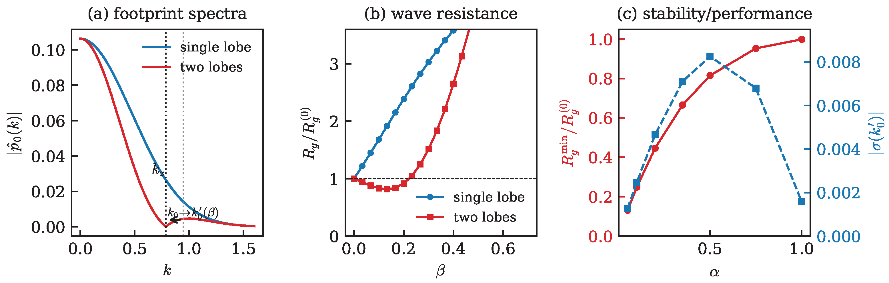
gives the response for the single-lobe footprint. Three features are simultaneous and unavoidable. The stationary wave is damped, $\sigma \left(k_0\right)<0$, as Theorem 2 guarantees for $\alpha >0$. The wavetrain attenuates downstream, $\kappa >0$. And yet both the emitted amplitude and the wave resistance increase monotonically by factors of 2.66 and 5.07, respectively.

The mechanism is transparent from (15) and (24). For $\beta >0$ the real part of the response term is positive, so ${\mathcal{D}}_R$ is raised and its zero moves down: $k_0^{\prime }$ falls from 0.9487 to 0.4309. For a Gaussian footprint, $|{\widehat{p}}_0|$ is monotone decreasing, so a redshift lands the resonance where the forcing has more spectral content, and $R_g\propto {\widehat{p}}_0{\left(k_0^{\prime }\right)}^2$ rises. Taking $\beta <0$ blueshifts the resonance and reduces the amplitude, but, by (22), it simultaneously makes $\sigma \left(k_0\right)>0$ and $R_g<0$, an unphysical energy-extracting state.

Corollary 2.

Suppose $|{\widehat{p}}_0|$ is monotone decreasing on $[0,\infty )$ and $|{\mathcal{D}}_R^{\prime }\left(k_0^{\prime }\right)|$ varies slowly. Then, within the stable regime $\alpha \beta >0$, dynamic curvature coupling cannot reduce the wave resistance: drag reduction requires $\alpha \beta <0$, which, by (22), entails linear instability of the stationary lee wave.

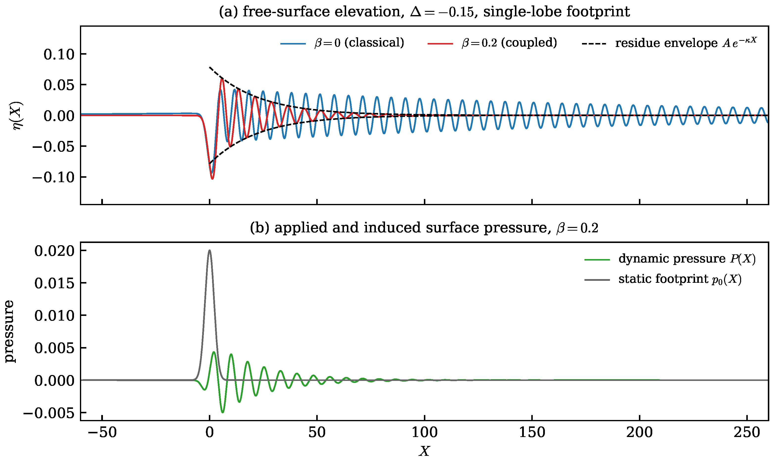
Figure 2 shows the corresponding surface profiles and the induced pressure field. The classical case radiates an undamped wavetrain; the coupled case radiates a larger wave that decays over a length $1/\kappa \approx 22$. The residue envelope (17) is superposed and is indistinguishable from the computed profile.

Corollary 2 is not a dead end but a design instruction. Its hypothesis is monotonicity of $|{\widehat{p}}_0|$; a stern footprint with two pressure lobes has ${\widehat{p}}_0\propto e^{-k^2{L}^2/4}\cos kd$, which vanishes at $k_z=\pi /\left(2d\right)$. Because the coupling shifts $k_0^{\prime }$ continuously downwards with $\beta$, one may steer the resonance onto the spectral zero. Classical wave-free solutions [15,16,17] achieve this by choosing the geometry for one operating condition; here $\beta$ provides a tunable knob that can track the zero as the Froude number changes.

Figure 3 and

Table 9. Optimal coupling for the two-lobe footprint, $\Delta =-0.15$ and $k_z=0.7853982$. Baseline $A_0=1.423998\times {10}^{-2}$ and $R_g^{\left(0\right)}=1.520828\times {10}^{-5}$. ${\beta }_{\mathrm{opt}}$ minimizes $R_g$.

$\mathit{\alpha }$	${\mathit{\beta }}_{\mathbf{opt}}$	${\mathit{k}}_0^{\prime }$	$\mathit{\kappa }$	${\mathit{R}}_{\mathit{g}}^{\min }/{\mathit{R}}_{\mathit{g}}^{\left(0\right)}$	$\mathit{A}/{\mathit{A}}_0$	$\mathit{\sigma }\left({\mathit{k}}_0^{\prime }\right)$
0.05	0.22584	0.792058	$5.051\times {10}^{-3}$	0.1314	0.0957	$-1.268\times {10}^{-3}$
0.10	0.21558	0.799143	$9.818\times {10}^{-3}$	0.2486	0.1892	$-2.475\times {10}^{-3}$
0.20	0.19503	0.814472	$1.831\times {10}^{-2}$	0.4461	0.3683	$-4.654\times {10}^{-3}$
0.35	0.16397	0.839691	$2.759\times {10}^{-2}$	0.6658	0.6085	$-7.106\times {10}^{-3}$
0.50	0.13238	0.866084	$3.146\times {10}^{-2}$	0.8150	0.7964	$-8.249\times {10}^{-3}$
0.75	0.07743	0.907636	$2.465\times {10}^{-2}$	0.9530	0.9629	$-6.795\times {10}^{-3}$
1.00	0.01551	0.942031	$5.360\times {10}^{-3}$	0.9987	0.9994	$-1.583\times {10}^{-3}$

show the outcome. The wave resistance now has a pronounced minimum at finite $\beta$, and the reduction is substantial: $R_g^{\min }/R_g^{\left(0\right)}=0.131$ at $\alpha =0.05$, i.e., an $87\%$ reduction, with the emitted amplitude falling to $9.6\%$ of its classical value. The state remains spectrally stable throughout, $\sigma \left(k_0^{\prime }\right)<0$.

The Performance–Strongness Trade-Off

Table 9 exhibits a systematic trend that admits an exact explanation. Steering cannot annihilate the wave completely because the pole $k_{\ast }=k_z+i\kappa$ sits off the real axis and ${\widehat{p}}_0\left(k_{\ast }\right)\ne 0$ even when ${\widehat{p}}_0\left(k_z\right)=0$. Expanding,

Theorem 4 (Residual radiation law).

At the steered condition ${\mathcal{D}}_R\left(k_z\right)=0$ with ${\widehat{p}}_0\left(k_z\right)=0$,

$$A=\kappa {\displaystyle \frac{|{\widehat{p}}_0^{\prime }\left(k_z\right)|}{|{\mathcal{D}}_R^{\prime }\left(k_z\right)|}}\left(1+O\left(\kappa \right)\right),\kappa ={\displaystyle \frac{\alpha \beta k_z^3\widehat{E}\left(k_z\right)}{2Q\left(k_z\right){\mathcal{D}}_R^{\prime }\left(k_z\right)}}.$$

(25)

Combining with Proposition 3 and Theorem 1,

$$A={\displaystyle \frac{k_z\left|{\widehat{p}}_0^{\prime }\left(k_z\right)\right|}{{\left(c_g^{\mathrm{eff}}\right)}^2}}\left|\sigma \left(k_z\right)\right|$$

(26)

so the residual radiated amplitude is directly proportional to the damping rate.

Equation (26) is the sharpest statement in the paper. It says that, within this closure, one cannot have both strong damping and complete wave cancellation: the very phase lag that extracts energy from the wave also displaces the pole from the real axis and so prevents the spectral zero from being reached exactly. Both effects scale with $\alpha \beta$.

Table 10. Verification of the residual radiation law (25) at the steered condition $k_0^{\prime }=k_z$ for a two-lobe footprint with $\Delta =-0.15$.

$\mathit{\alpha }$	${\mathit{\beta }}_{\ast }$	$\mathit{\kappa }$ (Numerical)	$\mathit{\kappa }$ (Formula)	A (Numerical)	A (Formula)
0.10	0.23726	$1.03705\times {10}^{-2}$	$1.03735\times {10}^{-2}$	$1.73336\times {10}^{-3}$	$1.73144\times {10}^{-3}$
0.20	0.24072	$2.08122\times {10}^{-2}$	$2.08348\times {10}^{-2}$	$3.50811\times {10}^{-3}$	$3.49230\times {10}^{-3}$
0.35	0.25024	$3.67601\times {10}^{-2}$	$3.68684\times {10}^{-2}$	$6.34078\times {10}^{-3}$	$6.24886\times {10}^{-3}$
0.50	0.26496	$5.32488\times {10}^{-2}$	$5.35085\times {10}^{-2}$	$9.51407\times {10}^{-3}$	$9.21377\times {10}^{-3}$
0.75	0.30102	$8.24864\times {10}^{-2}$	$8.29568\times {10}^{-2}$	$1.60447\times {10}^{-2}$	$1.47640\times {10}^{-2}$
1.00	0.35151	$1.14658\times {10}^{-1}$	$1.14671\times {10}^{-1}$	$2.50980\times {10}^{-2}$	$2.11575\times {10}^{-2}$

confirms (25) to $0.11\%$ at $\alpha =0.1$, degrading to $16\%$ at $\alpha =1$ where $\kappa$ is no longer small.

8. Validation and Convergence

Table 11. Three-way agreement. “residue” = Equation (17); “spectral” = FFT inversion, $L_{\mathrm{dom}}=6400$, and $N=2^{19}$; “marching” = time integration from rest, $N=2^{13}$, $\Delta \tau =0.02$, and ${\tau }_{\mathrm{end}}=1500$. The last row gives the relative $L^{\infty }$ difference between the marched and inverted profiles over the fitting window.

$\mathit{\beta }$	A			$\mathit{\kappa }$			${\mathit{k}}_{\mathit{r}}$
	Residue	Spectral	Marching	Residue	Spectral	Marching	Residue	Marching
0.05	5.21902$\times {10}^{-2}$	5.21790$\times {10}^{-2}$	5.16034$\times {10}^{-2}$	1.2257$\times {10}^{-2}$	1.2255$\times {10}^{-2}$	1.2121$\times {10}^{-2}$	0.917886	0.917951
0.20	7.83287$\times {10}^{-2}$	7.84221$\times {10}^{-2}$	7.89685$\times {10}^{-2}$	4.4336$\times {10}^{-2}$	4.4365$\times {10}^{-2}$	4.4531$\times {10}^{-2}$	0.821100	0.821162
0.50	1.11464$\times {10}^{-1}$	1.11184$\times {10}^{-1}$	1.12544$\times {10}^{-1}$	6.2585$\times {10}^{-2}$	6.2515$\times {10}^{-2}$	6.2844$\times {10}^{-2}$	0.655439	0.655375

relative $L^{\infty }\left(\eta \right)$: $4.18\times {10}^{-2}$ ($\beta =0.05$), $1.73\times {10}^{-2}$ ($\beta =0.20$), $1.27\times {10}^{-2}$ ($\beta =0.50$).

compares the closed-form residue evaluation, the spectral inversion and the time-marching solver. Emitted amplitudes agree to better than $1.1\%$, attenuation rates to better than $1.2\%$, and radiated wavenumbers to better than ${10}^{-4}$ relative. The pointwise $L^{\infty }$ discrepancy between the marched and inverted profiles is $1.3$–$4.2\%$, the larger value occurring at $\beta =0.05$ where the attenuation length $1/\kappa \approx 82$ is comparable with the usable domain.

For the uncoupled problem the marched amplitude is $4.378895\times {10}^{-2}$ against the closed form $A_0=4.438946\times {10}^{-2}$ of (16), a relative difference of $1.35\times {10}^{-2}$, and the measured wavenumber $0.94856439$ against $k_0=0.94868330$, a relative difference of $1.3\times {10}^{-4}$.

It is worth stating explicitly that the attenuation rates reported in Table 7, Table 8 and Table 9 are obtained from the residue evaluation, $\kappa =\mathrm{Im}{k}_{\ast }$, which involves no spatial domain, no truncation and no boundaries and is therefore free of any reflection effect by construction; the finite-domain computations serve as independent checks on that value rather than as its source. The check is most demanding at small $\beta$, where the attenuation length is longest. At $\beta =0.05$, for which $1/\kappa \approx 82$ is comparable with the usable domain, the spectral inversion differs from the residue value by $0.02\%$, and the time-marched value lies $1.1\%$ below it, so the finite-domain error at small $\beta$ biases $\kappa$ downwards rather than upwards. The residual domain dependence is in any case monotone and first order, the deviation halving at each doubling of $L_{\mathrm{dom}}$, which is the signature of truncation rather than of reflection from the sponge layers.

The sharp criterion of Theorem 2 is tested directly by seeding the unforced system with low-level noise on a periodic domain and measuring ${\tau }^{-1}\log |\widehat{\eta }(k,\tau )/\widehat{\eta }(k,0)|$.

Table 12. Measured versus predicted modal growth rates, $\beta =0.2$ and $k_c=1.974842$. Measurement from a noise-seeded run to $\tau =300$ on a periodic domain of length 200 with $N=2^{11}$.

$\mathit{k}$	${\mathit{k}}_{\mathit{b}}=1.6$ ($\le {\mathit{k}}_{\mathit{c}}$)		${\mathit{k}}_{\mathit{b}}=2.4$ ($>{\mathit{k}}_{\mathit{c}}$)		${\mathit{k}}_{\mathit{b}}=3.5$ ($>{\mathit{k}}_{\mathit{c}}$)
	Measured	Predicted	Measured	Predicted	Measured	Predicted
0.503	−2.8219$\times {10}^{-3}$	−2.8385$\times {10}^{-3}$	−3.0024$\times {10}^{-3}$	−3.0201$\times {10}^{-3}$	−3.0758$\times {10}^{-3}$	−3.0940$\times {10}^{-3}$
0.943	−1.3823$\times {10}^{-2}$	−1.3892$\times {10}^{-2}$	−1.9197$\times {10}^{-2}$	−1.9294$\times {10}^{-2}$	−2.1127$\times {10}^{-2}$	−2.1234$\times {10}^{-2}$
1.508	−2.1555$\times {10}^{-5}$	−2.1647$\times {10}^{-5}$	−2.4110$\times {10}^{-2}$	−2.4209$\times {10}^{-2}$	−2.8966$\times {10}^{-2}$	−2.9074$\times {10}^{-2}$
2.011	5.1$\times {10}^{-15}$	0	2.1134$\times {10}^{-3}$	2.1221$\times {10}^{-3}$	4.3320$\times {10}^{-2}$	4.3495$\times {10}^{-2}$
2.513	−9.5$\times {10}^{-15}$	0	−9.5$\times {10}^{-15}$	0	9.3563$\times {10}^{-2}$	9.3771$\times {10}^{-2}$
2.985	6.8$\times {10}^{-15}$	0	6.8$\times {10}^{-15}$	0	3.2651$\times {10}^{-2}$	3.2693$\times {10}^{-2}$

${\max }_k|\mathrm{measured}-\mathrm{predicted}|$: $7.18\times {10}^{-5}$, $1.35\times {10}^{-4}$, $2.35\times {10}^{-4}$.

shows agreement with the eigenvalue prediction to four significant figures and reproduces the predicted transition: for $k_b=1.6\le k_c$, every measured rate is non-positive, whereas, for $k_b=2.4>k_c$, a positive rate appears at $k\approx 2.01$, just above $k_c=1.9748$.

Table 13. Domain and resolution convergence of the spectral inversion, $\beta =0.20$. Residue reference values: $A=7.832871077914\times {10}^{-2}$, $\kappa =4.433610720911\times {10}^{-2}$, and $k_r=0.821099688731$.

${\mathit{L}}_{\mathbf{dom}}$	N	A	rel. dev.	$\mathit{\kappa }$	rel. dev.
400	$2^{14}$	$7.9850730\times {10}^{-2}$	$1.94\times {10}^{-2}$	$4.4802764\times {10}^{-2}$	$1.05\times {10}^{-2}$
800	$2^{15}$	$7.9082601\times {10}^{-2}$	$9.62\times {10}^{-3}$	$4.4567939\times {10}^{-2}$	$5.23\times {10}^{-3}$
1600	$2^{16}$	$7.8703736\times {10}^{-2}$	$4.79\times {10}^{-3}$	$4.4451605\times {10}^{-2}$	$2.61\times {10}^{-3}$
3200	$2^{17}$	$7.8515583\times {10}^{-2}$	$2.39\times {10}^{-3}$	$4.4393705\times {10}^{-2}$	$1.30\times {10}^{-3}$
6400	$2^{18}$	$7.8421824\times {10}^{-2}$	$1.19\times {10}^{-3}$	$4.4364821\times {10}^{-2}$	$6.48\times {10}^{-4}$
12,800	$2^{19}$	$7.8375024\times {10}^{-2}$	$5.91\times {10}^{-4}$	$4.4350395\times {10}^{-2}$	$3.22\times {10}^{-4}$

shows first-order convergence of the spectral inversion towards the residue values as the domain is enlarged, the truncation error halving at each doubling; Richardson extrapolation of the last two entries gives $A=7.8328\times {10}^{-2}$ against the residue value $7.832871\times {10}^{-2}$.

Table 14. Wave-resistance quadrature, $\beta =0.20$: convergence and the exact absorption identity (20). $N_k$ is the number of quadrature points; K is the truncation wavenumber.

$({\mathit{N}}_{\mathit{k}},\mathit{K})$	${\mathit{R}}_{\mathit{g}}$	${\mathit{R}}_{\mathit{g}}+{\mathit{R}}_{\mathit{d}}$
$(5\times {10}^5,40)$	$3.522186402082\times {10}^{-4}$	0
$(2\times {10}^6,40)$	$3.522186402082\times {10}^{-4}$	$-5.4\times {10}^{-20}$
$(8\times {10}^6,40)$	$3.522186402082\times {10}^{-4}$	0
$(4\times {10}^6,20)$	$3.522186402082\times {10}^{-4}$	0
$(4\times {10}^6,80)$	$3.522186402082\times {10}^{-4}$	0

shows that the wave-resistance quadrature is converged to 13 significant figures and independent of both the number of quadrature points and the truncation wavenumber, and identity (20) holds to machine zero. The marching scheme is likewise converged: $N=2^{12}$, $\Delta \tau =0.04$ gives $A=7.89623\times {10}^{-2}$ and $N=2^{13}$, $\Delta \tau =0.02$ gives $A=7.89685\times {10}^{-2}$, a difference of $8\times {10}^{-5}$ relative, so the residual $0.8\%$ offset from the residue value is a finite-domain effect that is consistent with Table 13, not a discretization error.

Finally we verify that the linearization is the correct leading order. The full system, nonlinear term retained, is marched at successively smaller forcing amplitudes and the normalized emitted amplitude $A/a$ compared with the linear prediction $A/a=3.916436$.

Table 15. Recovery of the linear prediction from the full nonlinear system, $\beta =0.20$. The departure is $O\left(a\right)$, confirming that the linear reduction is the correct leading-order description.

a	$\max \left|\mathit{\eta }\right|$	$\mathit{A}/\mathit{a}$ (Nonlinear)	Departure from Linear
$5.00\times {10}^{-3}$	$2.903\times {10}^{-2}$	4.895205	$2.499\times {10}^{-1}$
$2.50\times {10}^{-3}$	$1.365\times {10}^{-2}$	4.376020	$1.173\times {10}^{-1}$
$1.25\times {10}^{-3}$	$6.650\times {10}^{-3}$	4.158352	$6.177\times {10}^{-2}$

shows the departure halving as a halves, i.e., clean $O\left(a\right)$ convergence as required.

9. Discussion

The mathematical content of this paper is strong: Theorems 1–4 are exact statements about the system (2)–(5), verified independently. The modeling content requires more care, and we set out the boundaries explicitly.

Equation (5) is physically motivated but is not derived from a boundary-layer or wake model of a separated stern flow. The parameters $(\alpha ,\beta ,\gamma ,\delta ,k_b)$ are not yet connected to measurable quantities. Before any of the design statements of Section 7 could be taken seriously for a hull, they would need to be calibrated against RANS or experimental surface-pressure data, and the scaling requirements of Table 3—particularly the slow-drift condition $\alpha =O\left(ϵ\right)$ of Remark 2—would need to be checked against that data. In its actuated reading the model is on firmer ground since $(\alpha ,\beta ,\gamma ,\delta ,k_b)$ are then design parameters of a control system rather than unknowns of a turbulent flow.

The steering result relies on a spectral zero of the forcing, a linear notion. Table 15 shows that nonlinearity enters at $O\left(a\right)$ and that the linear prediction is recovered as $a\to 0$, but, at finite amplitude, the zero will be smeared and the achievable reduction degraded. Quantifying this requires a nonlinear continuation study of the kind performed by Keeler et al. [17] for the Kelvin wake and is the natural next step.

More generally, we stress that spectral stability of the linearized system does not imply nonlinear stability, still less the stability of a physical stern flow, and we claim neither. Theorem 3 is the one result that survives the nonlinearity intact since the absorption identity holds for any steady decaying solution of the full system and its proof nowhere uses linearity; the equivalence of passivity with stability, and every growth rate and stability margin quoted in this paper, are statements about the linearization. Table 15 establishes that the linearization is the correct leading-order description with the departure $O\left(a\right)$, but that is a statement about small amplitudes and not a nonlinear stability result. Establishing nonlinear stability would require the finite-amplitude continuation study just described, and physical stability would additionally require the transverse analysis discussed next.

Real sterns are three-dimensional; the extension is standard in principle but changes the spectral-zero structure substantially. In more than one spatial dimension the KdV balance is replaced by a Zakharov–Kuznetsov-type equation, whose solitary waves admit transverse instabilities with no one-dimensional counterpart [35]; whether the phase-lag damping identified here suppresses or merely reshapes that transverse growth is an open question and would have to be settled before the steering result of Section 7 could be transferred to a three-dimensional wake. We emphasize, since it bears directly on how the results should be used, that the stability margins $\left|\sigma \right(k_0^{\prime }\left)\right|$ reported in Table 9 are margins against one-dimensional disturbances only. The present model has no transverse degree of freedom, so it can neither predict nor exclude lateral instability, and no transverse growth rate should be inferred from it; we have deliberately not quoted one since any such figure would not be a consequence of the system analyzed here. Quantifying that risk requires the Zakharov–Kuznetsov extension described above, and we regard it, together with the finite-amplitude continuation study, as a prerequisite for any three-dimensional application. Separately, all the results are computed away from exact criticality ($\Delta =-0.15$, $k_0\approx 0.95$); as $\Delta \to 0^{-}$, the resonance approaches $k=0$, the group velocity vanishes, and the weakly nonlinear balance changes character. That limit needs separate treatment.

We do not claim wave elimination. Theorem 4 shows that exact cancellation is incompatible with nonzero damping within this closure and quantifies the residual. We do not claim a drag reduction for a general hull: Corollary 2 shows the opposite for the simplest footprint, and the favorable result of Table 9 depends on engineering a spectral zero into the footprint.

10. Conclusions

Promoting surface pressure from a prescribed function to a dynamic field with finite relaxation time fundamentally shifts the understanding of stern-flow problems by introducing relaxation dynamics effects that are mathematically sharp and physically interpretable. This model moves beyond traditional diagnostic closures by demonstrating that a pressure field’s finite response time and drift speed create a phase lag that is essential for energy transfer. The key theoretical results, including the Miles-type phase-speed criterion and the sharp bandwidth theorem, establish that the sign of energy transfer is decided by the comparison of pressure drift speed with intrinsic phase speed. Furthermore, the system enforces an exact energy identity where the dynamic field absorbs the work done by the applied pressure, proving that passivity and spectral stability are equivalent.

From a design perspective, the research highlights a significant performance–strongness trade-off mediated by resonance steering. While monotone footprints necessarily increase wave resistance under stable coupling, steering the resonance onto a spectral zero of a multi-lobe footprint can reduce the resistance to less than one-seventh of its classical value while maintaining linear stability. This finding transforms the coupling strength into a tunable parameter that is capable of tracking zeros as Froude numbers change, offering a constructive path toward active wave drag minimization.

Despite these advances, the current closure is phenomenological and situated within a two-dimensional weakly nonlinear regime. The response parameters are not yet tied to measurable physical quantities, and the influence of nonlinearity on the spectral zero remains to be fully quantified. Consequently, future research must prioritize a nonlinear continuation study, the extension to three-dimensional flows, and the calibration of the model against experimental or RANS-computed pressure data to bridge the gap between these mathematical results and strong naval design tools.

References

1. Vanden-Broeck, J.-M. Nonlinear stern waves. J. Fluid Mech. 1980, 96, 603–611. [Google Scholar] [CrossRef] [Scilit]
2. Binder, B.J. Steady free-surface flow at the stern of a ship. Phys. Fluids 2010, 22, 012104. [Google Scholar] [CrossRef] [Scilit]
3. Ogilat, O.; McCue, S.W.; Turner, I.W.; Belward, J.A.; Binder, B.J. Minimising wave drag for free surface flow past a two-dimensional stern. Phys. Fluids 2011, 23, 072101. [Google Scholar] [CrossRef] [Scilit]
4. McCue, S.W.; Stump, D.M. Linear stern waves in finite depth channels. Q. J. Mech. Appl. Math. 2000, 53, 629–643. [Google Scholar] [CrossRef] [Scilit]
5. McCue, S.W.; Forbes, L.K. Free-surface flows emerging from beneath a semi-infinite plate with constant vorticity. J. Fluid Mech. 2002, 461, 387–407. [Google Scholar] [CrossRef] [Scilit]
6. Farrow, D.E.; Tuck, E.O. Further studies of stern wavemaking. J. Austral. Math. Soc. Ser. B 1995, 36, 424–437. [Google Scholar] [CrossRef] [Scilit]
7. Binder, B.J.; Vanden-Broeck, J.-M.; Dias, F. On satisfying the radiation condition in free-surface flows. J. Fluid Mech. 2009, 624, 179–189. [Google Scholar] [CrossRef] [Scilit]
8. Kataoka, T.; Akylas, T.R. Steady radiating gravity waves: An exponential asymptotics approach. Water Waves 2024, 6, 79–102. [Google Scholar] [CrossRef] [Scilit]
9. Akylas, T.R. On the excitation of long nonlinear water waves by a moving pressure distribution. J. Fluid Mech. 1984, 141, 455–466. [Google Scholar] [CrossRef] [Scilit]
10. Wu, T.Y. Generation of upstream advancing solitons by moving disturbances. J. Fluid Mech. 1987, 184, 75–99. [Google Scholar] [CrossRef] [Scilit]
11. Grimshaw, R.H.J.; Maleewong, M. Transcritical flow over two obstacles: Forced Korteweg-de Vries framework. J. Fluid Mech. 2016, 809, 918–940. [Google Scholar] [CrossRef] [Scilit]
12. Grimshaw, R.H.J.; Maleewong, M. Transcritical flow over obstacles and holes: Forced Korteweg-de Vries framework. J. Fluid Mech. 2019, 881, 660–678. [Google Scholar] [CrossRef] [Scilit]
13. Binder, B.J. Steady two-dimensional free-surface flow past disturbances in an open channel: Solutions of the Korteweg-de Vries equation and analysis of the weakly nonlinear phase space. Fluids 2019, 4, 24. [Google Scholar] [CrossRef] [Scilit]
14. Binder, B.J.; Dias, F.; Vanden-Broeck, J.-M. Steady free-surface flow past an uneven channel bottom. Theor. Comput. Fluid Dyn. 2006, 20, 125–144. [Google Scholar] [CrossRef] [Scilit]
15. Michalski, H.; Mattner, T.; Balasuriya, S.; Binder, B.J. The effect of obstacle length and height in subcritical free-surface flow. Theor. Comput. Fluid Dyn. 2024, 38, 511–530. [Google Scholar] [CrossRef] [Scilit]
16. Robbins, C.; Blyth, M.G.; Maclean, J.; Binder, B.J. A method to calculate inverse solutions for steady open channel free-surface flow. J. Fluid Mech. 2023, 977, A46. [Google Scholar] [CrossRef] [Scilit]
17. Keeler, J.S.; Binder, B.J.; Blyth, M.G. Towards eliminating the nonlinear Kelvin wake. J. Fluid Mech. 2025, 1013, A10. [Google Scholar] [CrossRef] [Scilit]
18. Tuck, E.O.; Lazauskas, L. Free-surface pressure distributions with minimum wave resistance. ANZIAM J. 2001, 43, E75–E101. [Google Scholar] [CrossRef] [Scilit]
19. Flamarion, M.V.; Pelinovsky, E. Solitary wave interactions with an external periodic force: The extended Korteweg-de Vries framework. Mathematics 2022, 10, 4538. [Google Scholar] [CrossRef] [Scilit]
20. Flamarion, M.V.; Ribeiro, R., Jr.; Vianna, D.L.S.S.; Sato, A.M. Trapped solitary waves in a periodic external force: A numerical investigation using the Whitham equation and the sponge layer method. Fluids 2023, 8, 223. [Google Scholar] [CrossRef] [Scilit]
21. Flamarion, M.V.; Pelinovsky, E.; Melnikov, I. Spring-mass behavior of solitons under the influence of an external force field within the modified Korteweg-de Vries equation. Chaos Solitons Fractals 2025, 196, 116422. [Google Scholar] [CrossRef] [Scilit]
22. Melnikov, I.; Flamarion, M.V. Soliton dynamics under the influence of an external force and induced-damped terms within the modified Korteweg-de Vries equation. Nonlinear Dyn. 2026, 114, 42. [Google Scholar] [CrossRef] [Scilit]
23. Martins, L.G.; Flamarion, M.V.; Ribeiro-Jr, R. A forced Boussinesq model with a sponge layer. Partial Differ. Equ. Appl. Math. 2024, 10, 100661. [Google Scholar] [CrossRef] [Scilit]
24. Camassa, R.; Wu, T.Y. Stability of some stationary solutions for the forced KdV equation. Physica D 1991, 51, 295–307. [Google Scholar] [CrossRef] [Scilit]
25. Grimshaw, R.; Pelinovsky, E.; Tian, X. Interaction of a solitary wave with an external force. Physica D 1994, 77, 405–433. [Google Scholar] [CrossRef] [Scilit]
26. Zdyrski, T.; Feddersen, F. Wind-induced changes to surface gravity wave shape in shallow water. J. Fluid Mech. 2021, 903, A27. [Google Scholar] [CrossRef] [Scilit]
27. Jeffreys, H. On the formation of water waves by wind. Proc. R. Soc. Lond. A 1925, 107, 189–206. [Google Scholar] [CrossRef] [Scilit]
28. Maleewong, M.; Grimshaw, R. Evolution of water wave packets by wind in shallow water. J. Fluid Mech. 2024, 996, A4. [Google Scholar] [CrossRef] [Scilit]
29. Maleewong, M.; Grimshaw, R. Evolution of wind-generated shallow-water waves in the framework of a modified Kadomtsev-Petviashvili equation. Fluids 2025, 10, 61. [Google Scholar] [CrossRef] [Scilit]
30. Miles, J.W. On the generation of surface waves by shear flows. J. Fluid Mech. 1957, 3, 185–204. [Google Scholar] [CrossRef] [Scilit]
31. Hussain, A.; Hammad, M.; Rahimzai, A.A.; Koh, W.S.; Khan, I. Dynamical analysis and soliton solutions of the space–time fractional Kaup–Boussinesq system. Partial Differ. Equ. Appl. Math. 2025, 14, 101205. [Google Scholar] [CrossRef] [Scilit]
32. Gaster, M. A note on the relation between temporally-increasing and spatially-increasing disturbances in hydrodynamic stability. J. Fluid Mech. 1962, 14, 222–224. [Google Scholar] [CrossRef] [Scilit]
33. Trefethen, L.N. Spectral Methods in MATLAB; SIAM: Philadelphia, PA, USA, 2000. [Google Scholar]
34. Kassam, A.-K.; Trefethen, L.N. Fourth-order time-stepping for stiff PDEs. SIAM J. Sci. Comput. 2005, 26, 1214–1233. [Google Scholar] [CrossRef] [Scilit]
35. Gwaily, S.A.; Altuijri, R.; Nisar, K.S.; Abdel-Aty, A.-H.; Atteya, A.; El-Bayoumi, E.M. Nonlinear dust-acoustic solitons and multidimensional instabilities in magnetized plasmas with superthermal ions: A Zakharov–Kuznetsov framework. Braz. J. Phys. 2025, 55, 196. [Google Scholar] [CrossRef] [Scilit]
Figure 1. (a) Growth rate σ ( k ) for β = 0.2 and several response bandwidths; the vertical dotted lines mark k 0 and k c . Stability holds precisely while k b k c . (b) Unregularized coupling, E ^ 1 : the growth rate saturates at 3 β (dotted) rather than diverging, so the problem is uniformly unstable but well posed.
Mathematics 14 03245 g001
Figure 2. (a) Free-surface elevation for the classical ( β = 0 ) and coupled ( β = 0.2 ) problems, together with the residue envelope ± A e κ X of (17). The upstream region is wave-free, confirming that the radiation condition is satisfied. (b) The static footprint p 0 and the induced dynamic pressure P for β = 0.2 ; note that P extends far downstream over the whole attenuating wavetrain.
Mathematics 14 03245 g002
Figure 3. (a) Spectra of the single- and two-lobe footprints; the coupling redshifts the resonance from k 0 towards the spectral zero k z . (b) Wave resistance against coupling strength: monotone increase for the monotone spectrum; pronounced minimum for the two-lobe footprint. (c) The performance–strongness trade-off: the attainable resistance reduction (left axis) and the stability margin | σ ( k 0 ) | (right axis) both scale with the drift speed α .
Mathematics 14 03245 g003