Reliability and Profit Analysis of a Five-Subsystem Hybrid Series-Parallel System with Gumbel–Hougaard Copula Repair, Cold Standby, and Dual Environmental Failure Rates

Abstract

This work offers a reliability framework for a five-subsystem hybrid series-parallel system representing smart factory monitoring infrastructure under heat and vibration stressors. A central programmable logic controller (1-out-of-1), pressure and temperature sensors (2-out-of-5), wireless communication units (2-out-of-4), solar power modules (3-out-of-6), and a cold standby database server (1-out-of-2) are connected in series. Unit failures are modeled using exponential distributions with component-specific failure rates and two environmental failure rates for thermal stress (${\alpha }_6$) and vibration stress (${\alpha }_7$) which go beyond the single-parameter models used in prior research. Repair of degraded states is governed by general distributions. The Gumbel–Hougaard copula family deals with total failure states, permitting positive repair time dependence due to common maintenance resources and environmental recovery. The state probabilities are obtained in closed form by using Laplace transforms and the supplementary variable method. Those state probabilities are used to find system availability, reliability, $MTTF$, sensitivity, indices and profit for three cases: copula-based repair, general distribution repair and a reduction technique with parameter $\rho$. Numerical analysis reveals steady state availability of 96.80%when using copula repair, and 99.35% when using the reduction technique ($\rho$ = 0.2). Sensitivity analysis reveals that the solar power module subsystem is the main cause of $MTTF$ degradation, however cost analysis reveals that proactive quality enhancement is more profitable than reactive repair options at all maintenance expenditure levels.

1. Introduction

Modern industrial plants increasingly rely on smart factory technologies that integrate distributed sensor networks, wireless communication systems, programmable control devices, and renewable energy sources into unified monitoring systems. These systems must operate continuously in thermally harsh, mechanically demanding, and logistically challenging environments, where even a temporary failure can cause production outages, safety incidents, or irrecoverable data loss. Reliability is therefore not merely a technical metric but a key driver of operational and financial performance. Because such infrastructures combine subsystems with different redundancy requirements, failure modes, and repair logistics, traditional single-component or homogeneous reliability models are inadequate, motivating the development of hybrid system models that jointly capture structural redundancy, stochastic failure behavior, and maintenance dynamics.

The main structural feature of the system we study here is heterogeneous redundancy, which is represented by a series connection of mixed k-out-of-n:G structures. A k-out-of-n:G subsystem is said to be operational if at least k out of the n units are operational and it can tolerate at most n-k simultaneous failures. Since different subsystems of the same installation generally need different (k, n) pairs depending on their criticality, redundancy cost, and performance requirements, the heterogeneity among the central controller, sensor arrays, communication units, power modules, and cold standby data server should be taken into account in a realistic model of a smart factory monitoring system. Shi et al. [1] conducted a statistical analysis of a k/n:G system with dependent competing failure mechanisms governed by the Gumbel–Hougaard copula under progressively hybrid censored test data. Additionally, they applied the IFM marginal inference method for parameter estimation, extending copula reliability modeling into the statistical inference and censored data domain. Singh et al. [2] proposed a copula linguistic technique for performance and effectiveness assessment of a redundant k-out-of-n:G system with multiple consecutive degraded states. They also demonstrated that modeling successive degradation levels through copula repair substantially improves the accuracy of availability and profit estimates. Elshoubary et al. [3] modeled the Apache Kafka data streaming system as a series of four subsystems under the k-out-of-nn:G rule and compared general distribution repair against Gumbel–Hougaard copula repair and applied the reduction technique to improve all reliability metrics. Elshoubary et al. [4] proposed a series-parallel system of four subsystems with heterogeneous k-out-of-n configurations and copula-based repair. They used the supplementary variable technique and Laplace transforms to derive availability, $MTTF$, sensitivity, and profit. Elshoubary et al. [5] applied a four-subsystem framework specifically to a hybrid wireless sensor network in agricultural and industrial environments, evaluating the impact of copula-based repair versus general repair on availability and expected profit and demonstrating that copula repair consistently outperforms general repair across all reliability metrics. Chopra et al. [6] examined availability and reliability of a two-unit parallel network using Gumbel–Hougaard copula repair. This demonstrated that copula-modeled repair dependence consistently produces better reliability estimates than independence assumptions in parallel redundancy configurations. Ibrahim et al. [7] established reliability modeling based on the Gumbel–Hougaard copula for a two-system series configuration, evaluating availability, reliability, $MTTF$, and sensitivity, providing one of the foundational applications of the copula repair methodology in the series-parallel reliability literature. Singh et al. [8] analyzed a two-subsystem series system with an imperfect switch, deriving reliability metrics including availability, $MTTF$, and profit under copula and general repair policies. This work demonstrated that imperfect switching significantly degrades system performance and that copula repair partially compensates for switch-induced degradation. Singh et al. [9] provided a probabilistic assessment of a computer-based test network system using copula linguistic approach, evaluating state probabilities, availability, reliability, and $MTTF$ for a multi-subsystem configuration and establishing the use of copula-based repair in educational and networked computing systems. Ram et al. [10] analyzed a three-subsystem mixed series-parallel system with a 1-out-of-2:G subsystem and perfect reworking after repair. This work derived availability, reliability, $MTTF$, sensitivity, and cost-effectiveness using the Markov process and a supplementary variable technique, establishing the analytical template widely adopted in subsequent copula repair studies. Singh et al. [11] derived the availability, $MTTF$, and cost function for a two-unit series system with a controller, using the supplementary variable technique and Laplace transforms. This work established one of the core methodological references for series system reliability analysis with controller components. Wu et al. [12] analyzed a two-component cold standby repairable system with multiple failure modes using Markov renewal processes and Laplace–Stieltjes transforms, deriving closed-form expressions for mean time to first failure, steady-state availability, and rate of occurrence of failures. Zhang et al. [13] studied a semi-Markov cold standby system with two heterogeneous components and multiple failure modes using supplementary variable techniques. They showed that component quality differences have a large impact on both $MTTF$ and steady-state availability, and thus the failure rates of the primary and standby units should be parameterized differently. Shen et al. [14] considered a stochastic analysis of a two unit cold standby system with imperfect switching, and each unit was represented by three states: normal, partial failure, and total failure. They showed that the reliability of switching has a significant effect on system $MTTF$ and availability. Roy et al. [15] obtained reliability and availability for a 1-out-of-n cold standby redundant system with the generalized Lindley distribution, thus generalizing the cold standby modeling beyond the assumptions of exponential failure. Kumar et al. [16] studied hot and cold standby arrangements in three unit parallel systems using semi-Markov and regenerative point approaches. They found that if the failure rates of the units are equal, cold standby is always better than hot standby in a number of reliability criteria. In [17], Kumar et al. proposed a continuous-time Markov process model for reliability of WSN with sensing devices, transceivers, microcontrollers, power supplies and standby power supplies through failure and repair transitions. They assessed reliability, component specific reliability, mean time to failure ($MTTF$), and conducted sensitivity analysis. Heidari et al. [18] evaluated the reliability and availability of industrial wireless sensor networks in the presence of permanent failures using fault tree and Markov chain analysis. They analyzed possible cases of redundancy in active and idle states, demonstrating the importance of network device backup systems for reliable operation during long-term fault conditions in industrial environments. Ma et al. [19] proposed a new algorithm for reliability evaluation of linear wireless sensor network topology. The algorithm addresses a problem in the linear topology where the survival status of a single node determines the reliability of the network. Alavi et al. [20] evaluated the reliability of a grid-connected photovoltaic inverter in three degradation scenarios in hot–dry, hot–humid and moderate climate zones. The reliability of wireless sensor networks in harsh agricultural and industrial environments was considered by Catelani et al. [21] in relation to node deployment, redundancy configuration and communication protocol. Li et al. [22] studied a heterogeneous multi-component system with gradual degradation (described by Gamma processes) and random external shocks, where inspection and maintenance necessitate specialized crews on a component-by-component basis.

1.1. Gaps in the Existing Literature

The paper proposes a framework for reliability and profit analysis of a five-subsystem hybrid series-parallel system, motivated by smart factory monitoring infrastructure subject to thermal and vibrational stress. The proposed framework couples five heterogeneous k-out-of-n:G subsystems (including a cold standby configuration), dual environmental failure rates for thermal and vibrational stress, and a hybrid repair structure of general distribution repair for degraded states with Gumbel–Hougaard copula repair for complete failure states, unlike earlier multi-subsystem reliability studies which are generally limited to two-, three-, or four-subsystem configurations with a single aggregate environmental failure parameter and either copula-based or independent repair, but seldom both in a single model. Using Laplace transforms and the supplementary variable technique, we derive closed-form expressions for availability, reliability, $MTTF$, sensitivity indices and expected profit under three scenarios, namely, copula-based repair, general repair and a failure rate reduction technique, thus quantifying the relative value of dependent-repair modeling versus proactive component-quality improvement for the first time in a five-subsystem setting. This directly tackles the four gaps identified below: the absence of five-subsystem heterogeneous models, the absence of a unified copula/general-repair framework, the limited consideration of cold standby in copula-based multi-subsystem models, and the use of a single aggregate environmental failure parameter.

1.2. Research Objectives and Main Contributions

This paper fills these gaps by proposing a unified reliability framework for a five-subsystem hybrid series-parallel system that considers the monitoring infrastructure of a smart factory, integrating reliability block diagram and fault tree analysis to capture simultaneously the series-parallel topology and the logical failure dependencies. We show that degraded states are repaired under general distributions and that fully failed states are repaired under Gumbel–Hougaard copula based joint distributions that exhibit positive repair time dependence due to common maintenance resources. The cold standby unit in the database server subsystem is modeled as being zero failure rate when idle and a constant exponential rate when activated.

The main contributions are: (1) a unified five-subsystem model with truly heterogeneous k-out-of-n configurations—(1-out-of-1), (2-out-of-5), (2-out-of-4), (3-out-of-6), and (1-out-of-2) cold standby; (2) a combined analytical treatment of Gumbel–Hougaard copula repair and general-distribution repair within a single five-subsystem framework; (3) decomposition of environmental failure into distinct thermal (${\alpha }_6$) and vibrational (${\alpha }_7$) stressors, enabling subsystem-specific environmental sensitivity analysis; and (4) closed-form expressions for availability, reliability, $MTTF$, sensitivity indices, and expected profit under three scenarios—copula-based repair, general-distribution repair, and a component-quality reduction method that provides a complete assessment of system reliability and economic performance.

The rest of the paper is organized as follows. Section 2 describes the system architecture, the state space, assumptions and notation. The mathematical model and the Laplace transform representations for the state probabilities are derived in Section 3. Section 4 contains the results of the availability, reliability, $MTTF$, sensitivity, and cost analysis for the three scenarios. Section 5 concludes and discusses future research.

2. System Architecture, Assumptions, and Notations

2.1. System Architecture

We study a smart factory monitoring framework whose operation is continuous even under heat stress, mechanical vibration and complex maintenance logistics. The system is composed of five functionally independent subsystems, connected in series. For the system to be functional, all subsystems must simultaneously reach their minimum performance thresholds. The subsystems are implemented with heterogeneous k-out-of-n:G redundancy configurations, taking into account the different criticality levels and redundancy requirements of each functional layer.

• Subsystem 1—Central Programmable Logic Controller (1-out-of-1). SS1 is the computational and coordinating hub of the system. It implements the control logic, aggregates sensor data, and manages communications between all other subsystems. There is no redundant unit. So, SS1 is the single point of failure for the entire system. If it fails, the entire system is instantly useless. The design acknowledges that duplicating a central PLC presents synchronization problems that are greater than the benefits of increased reliability in many industrial applications. The failure rate of one unit is ${\alpha }_1$ = 0.02.
• Subsystem 2—Pressure and Temperature Sensors (2-out-of-5). SS2 has five sensing units and at least two of them have to be functional for the subsystem to meet its monitoring responsibilities. The degree of this redundancy is chosen to allow for sensor drift, fouling, or localized thermal degradation and to ensure sufficient measurement diversity for robust process control. Individual unit failure rate is ${\alpha }_2$ = 0.03.
• Subsystem 3—Wireless Communication Units (2-out-of-4). SS3 comprises four wireless transceivers, with a minimum of two required to stay operational for the continuity of data transfer within the monitoring network. The 2-out-of-4 threshold reconciles communication bandwidth demands with fault tolerance, guaranteeing that a solitary unit failure or interference incident does not disrupt system-wide data transmission. The failure rate of an individual unit is ${\alpha }_3$ = 0.04.
• Subsystem 4—Solar Power Modules (3-out-of-6). SS4 supplies electricity to the system via six photovoltaic modules, with a minimum of three required to stay operational to meet the essential power load for system functionality. This subsystem exhibits the highest individual unit failure rate (${\alpha }_4$ = 0.05) and is subjected to thermal and vibrational stressors, establishing it as the most reliability-critical subsystem, as corroborated by the sensitivity analysis. The 3-out-of-6 design incorporates a major redundancy buffer to permit partial shade, thermal derating or mechanical damage to individual panels without a rapid power loss.
• Subsystem 5—Cold Standby Database Server (1 of 2). SS5 consists of a main database server and a cold standby unit. In normal operation, the primary unit is online, and the standby unit is completely unpowered and hence does not fail when it is off. The backup unit is switched on when the primary unit fails and takes over the full operational responsibility. The backup unit is then subject to the normal unit failure rate ${\alpha }_5$ = 0.03. This cold standby arrangement secures the data logging and retrieval functions of the system, which is the most sensitive layer of the architecture concerning data integrity, without the cost and complexity of a fully active parallel system.

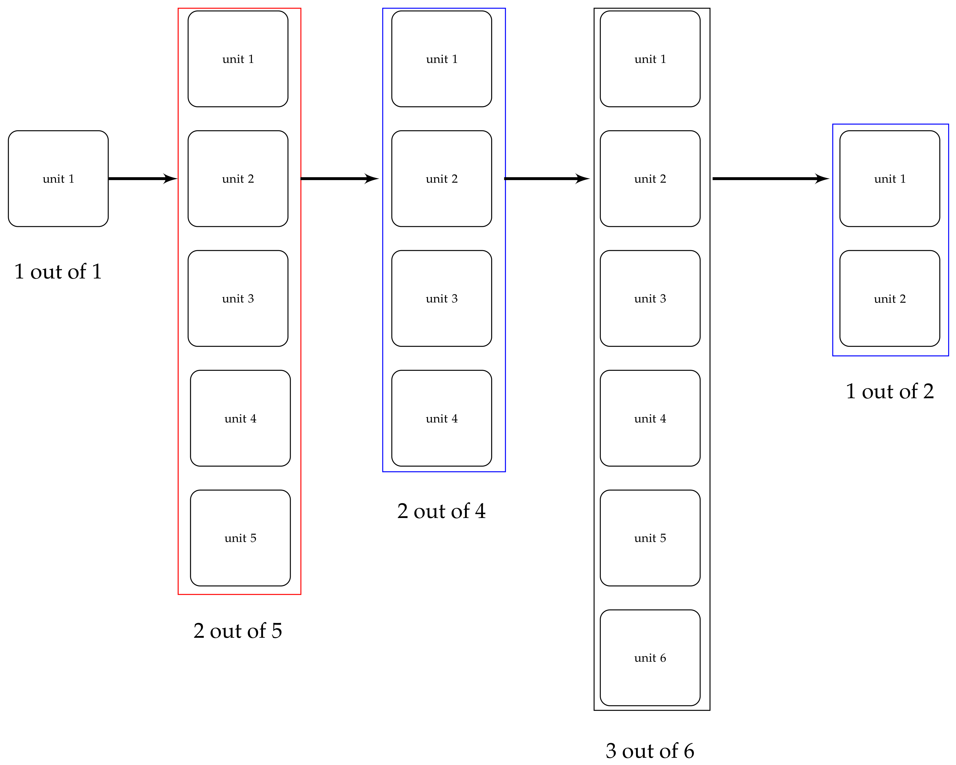
The five subsystems are in series, at the system level, as shown in Figure 1. The system is affected by two simultaneous environmental failure rates: ${\alpha }_6$ for thermally induced failures due to temperature variations and humidity, affecting all subsystems, and ${\alpha }_7$ for mechanically induced failures due to vibration and shock. Both ${\alpha }_6$ and ${\alpha }_7$ are system-wide competing environmental hazards applied uniformly, impacting all subsystems equally, compared to subsystem-targeted stressors. The two-parameter environmental model presented here is an explicit architectural improvement over the single aggregate environmental rate used previously, allowing for different physical interpretations and targeted mitigation techniques for each failure mechanism.

Table 1. Configurations of subsystems, industrial functions, and baseline failure rates of units for the five-subsystem hybrid series-parallel monitoring system.

Subsystem	Configuration	Industrial Role	Failure Rate
SS1	1-out-of-1	Central PLC/gateway	${\delta }_1$= 0.02
SS2	2-out-of-5	Pressure temperature sensors	${\delta }_2$ = 0.03
SS3	2-out-of-4	Wireless communication units	${\delta }_3$ = 0.04
SS4	3-out-of-6	Solar power modules	${\delta }_4$ = 0.05
SS5	1-out-of-2 (Cold Standby)	Database server (primary + backup)	${\delta }_5$ = 0.03

describes the configuration, industrial function and baseline failure rate of each subsystem.

2.2. State Space

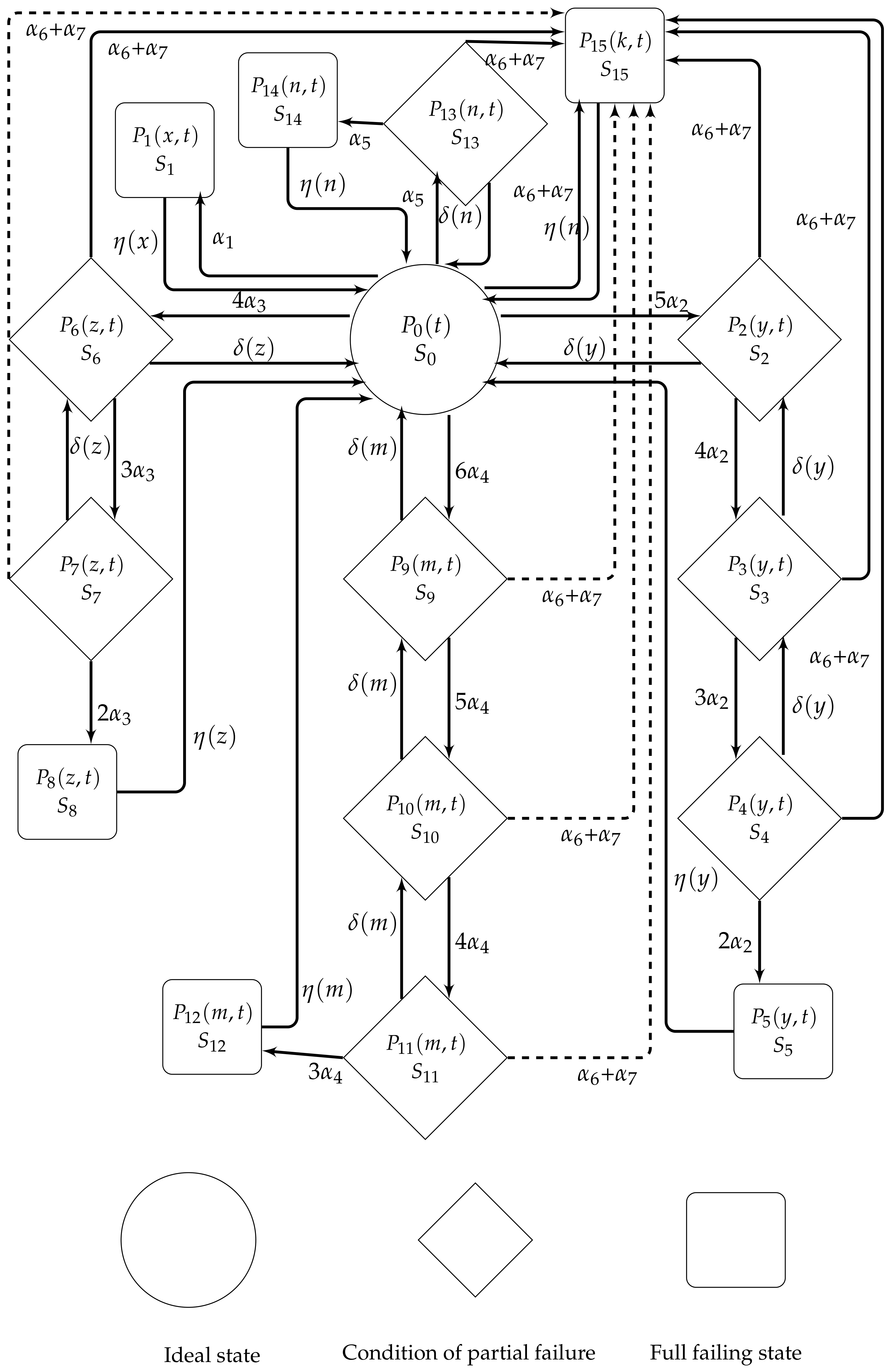
The system encompasses a total of 16 states: one completely operating state ($S_0$), nine degraded-but-functional stages ($S_2$, $S_3$, $S_4$, $S_6$, $S_7$, $S_9$, $S_{10}$, $S_{11}$, $S_{13}$), and six complete failure states ($S_1$, $S_5$, $S_8$, $S_{12}$, $S_{14}$, $S_{15}$, along with two environmental failure states). Note that the system enters state $S_{15}$ after the first of the two environmental failure events to occur, not after the joint occurrence of both.

Table 2. System state classification, operational delineation and designated remedial model for each of the sixteen system states, distinguishing between fully operational, degraded-but-functional and complete failure conditions.

State(s)	Type	Description	Repair Model
$S_0$	Operational	All components fully functional	N/A
$S_2$, $S_3$, $S_4$	Degraded	1, 2, or 3 units failed in SS2 (2/5 still met)	General Repair
$S_6$, $S_7$	Degraded	1 or 2 units failed in SS3 (2/4 still met)	General Repair
$S_9$, $S_{10}$, $S_{11}$	Degraded	1, 2, or 3 units failed in SS4 (3/6 still met)	General Repair
$S_{13}$	Degraded	SS5 cold standby active; partial degradation	General Repair
$S_1$	Failed	SS1 (PLC) complete failure	Gumbel Copula
$S_5$, $S_8$, $S_{12}$	Failed	Complete failure of SS2, SS3, or SS4	Gumbel Copula
$S_{14}$	Failed	SS5 complete failure (both units)	Gumbel Copula
$S_{15}$	Failed	Combined environmental failure (${\alpha }_6$ + ${\alpha }_7$)	Gumbel Copula

summarizes the definitions of the states.

2.3. Assumptions

We made the following assumptions while developing the model:

• All subsystems are initially fully operational ($P_0(0)$ = 1).
• There is a correlation between unit failures and exponential distributions, which are characterized by constant rates.
• Repair methodologies conform to standard distributions for deteriorated circumstances and employ Gumbel Copula-based joint distributions for complete failure scenarios.
• The cold standby unit in SS5 demonstrates a failure rate of zero during standby mode; upon activation, its failure rate increases to ${\alpha }_5$.
• Following the repair of the Gumbel Copula, the system returns to a fully operational state $S_0$, in accordance with the as-good-as-new hypothesis.
• The environmental failure rates ${\alpha }_6$ and ${\alpha }_7$ concurrently and independently affect all subsystems.

3. The Related Solution and the Mathematical Model

Utilizing the transition structure depicted in Figure 2 and the principles of Markov process theory, we formulated a system of first-order partial differential equations that regulate the state probabilities.

$$\begin{array}{c}\hfill \left[{\displaystyle \frac{d}{dt}}+{\alpha }_1+5{\alpha }_2+4{\alpha }_3+6{\alpha }_4+{\alpha }_5+{\alpha }_6+{\alpha }_7\right]P_0(t)={\int }_0^{\infty }\delta (y)P_2(y,t)dy+{\int }_0^{\infty }\delta (z)P_6(z,t)dz\\ \hfill +{\int }_0^{\infty }\delta (m)P_9(m,t)dm+{\int }_0^{\infty }\eta (x)P_1(x,t)dx+{\int }_0^{\infty }\eta (y)P_5(y,t)dy+{\int }_0^{\infty }\eta (z)P_8(z,t)dz\\ \hfill +{\int }_0^{\infty }\eta (m)P_{12}(m,t)dm+{\int }_0^{\infty }\eta (n)P_{14}(n,t)dn+{\int }_0^{\infty }\eta (k)P_{15}(k,t)dk\end{array}$$

(1)

Equation (1) is the master balance equation for the state $S_0$ of the fully operational state. The left-hand side is the total instantaneous rate at which the system leaves $S_0$, i.e., the sum of all unit-level failure rates across the five subsystems plus the two environmental stress rates ${\alpha }_6$, ${\alpha }_7$. The right-hand side is the total return flow to $S_0$. The first three integrals are the total return flow from completed repairs from degraded (but still functional) states in SS2, SS3 and SS4 under the general repair rate $\delta (x)$, and the remaining integrals are the total return flow from completed copula-based repairs from every total-failure state ($S_1,S_5,S_8,S_{12},S_{14},S_{15}$) under $\eta (y)$. Physically, this equation states that the system can be brought back to full operation only after either a partial degradation is repaired, or a total failure is jointly restored.

The first-order partial differential Equations (2)–(16) are derived using the supplementary variable technique. The supplementary variable (x, y, z, m, or n) is the time elapsed since entering that state undergoing repair. This formulation is what permits the repair to be generally (non-exponentially) distributed rather than restricted to the memory-less Markov assumption. In each equation, the coefficient of $P_i$ is the total ’hazard’ of leaving this state, either by more unit failures pushing the subsystem further into degradation (e.g., $4{\alpha }_2$ in Equation (3)), environmental stress (${\alpha }_6+{\alpha }_7$), or end of repair ($\delta (x)$, $\eta (y)$). The equations in Equations (2), (6), (9), (13) and (16) (the states ($S_1,S_5,S_8,S_{12},S_{14},S_{15}$)) with no further degradation path available) use only $\eta (y)$, as these are complete-failure states repaired only via the copula joint distribution.

$$\left[{\displaystyle \frac{\partial }{\partial t}}+{\displaystyle \frac{\partial }{\partial x}}+\eta (x)\right]P_1(x,t)=0$$

(2)

$$\left[{\displaystyle \frac{\partial }{\partial t}}+{\displaystyle \frac{\partial }{\partial y}}+4{\alpha }_2+{\alpha }_6+{\alpha }_7+\delta (y)\right]P_2(y,t)=0$$

(3)

$$\left[{\displaystyle \frac{\partial }{\partial t}}+{\displaystyle \frac{\partial }{\partial y}}+3{\alpha }_2+{\alpha }_6+{\alpha }_7+\delta (y)\right]P_3(y,t)=0$$

(4)

$$\left[{\displaystyle \frac{\partial }{\partial t}}+{\displaystyle \frac{\partial }{\partial y}}+2{\alpha }_2+{\alpha }_6+{\alpha }_7+\delta (y)\right]P_4(y,t)=0$$

(5)

$$\left[{\displaystyle \frac{\partial }{\partial t}}+{\displaystyle \frac{\partial }{\partial y}}+\eta (y)\right]P_5(y,t)=0$$

(6)

$$\left[{\displaystyle \frac{\partial }{\partial t}}+{\displaystyle \frac{\partial }{\partial z}}+3{\alpha }_3+{\alpha }_6+{\alpha }_7+\delta (z)\right]P_6(z,t)=0$$

(7)

$$\left[{\displaystyle \frac{\partial }{\partial t}}+{\displaystyle \frac{\partial }{\partial z}}+2{\alpha }_3+{\alpha }_6+{\alpha }_7+\delta (z)\right]P_7(z,t)=0$$

(8)

$$\left[{\displaystyle \frac{\partial }{\partial t}}+{\displaystyle \frac{\partial }{\partial z}}+\eta (z)\right]P_8(z,t)=0$$

(9)

$$\left[{\displaystyle \frac{\partial }{\partial t}}+{\displaystyle \frac{\partial }{\partial m}}+5{\alpha }_4+{\alpha }_6+{\alpha }_7+\delta (m)\right]P_9(m,t)=0$$

(10)

$$\left[{\displaystyle \frac{\partial }{\partial t}}+{\displaystyle \frac{\partial }{\partial m}}+4{\alpha }_4+{\alpha }_6+{\alpha }_7+\delta (m)\right]P_{10}(m,t)=0$$

(11)

$$\left[{\displaystyle \frac{\partial }{\partial t}}+{\displaystyle \frac{\partial }{\partial m}}+3{\alpha }_4+{\alpha }_6+{\alpha }_7+\delta (m)\right]P_{11}(m,t)=0$$

(12)

$$\left[{\displaystyle \frac{\partial }{\partial t}}+{\displaystyle \frac{\partial }{\partial m}}+\eta (m)\right]P_{12}(m,t)=0$$

(13)

$$\left[{\displaystyle \frac{\partial }{\partial t}}+{\displaystyle \frac{\partial }{\partial n}}+{\alpha }_5+\alpha (n)\right]P_{13}(n,t)=0$$

(14)

$$\left[{\displaystyle \frac{\partial }{\partial t}}+{\displaystyle \frac{\partial }{\partial n}}+\eta (n)\right]P_{14}(n,t)=0$$

(15)

$$\left[{\displaystyle \frac{\partial }{\partial t}}+{\displaystyle \frac{\partial }{\partial k}}+\eta (k)\right]P_{15}(k,t)=0$$

(16)

Boundary Conditions:

The boundary conditions for the above PDEs are given by Equations (17)–(31) with zero elapsed repair time (x = y = z = m = n = 0). They specific the rate of entry into each state, i.e., the probability mass that enters at the beginning of a new repair episode. Physically, each boundary condition adds two possible sources: (i) a direct failure transition from the previous (less-degraded) state, and (ii) in several cases, an indirect contribution from a deeper degraded state whose partial repair brings the subsystem back to a shallower degradation level (the integral terms in Equations (18), (19), (22), (25) and (26)). Equation (31) has a different structure: it adds the total environmental failure rate (${\alpha }_6$ + ${\alpha }_7$) that acts simultaneously on the fully operational state and on all degraded states, and that represents the assumption that the thermal and vibrational stress can cause a total environmental failure event ($S_{15}$) from any operating condition and not only from $S_0$.

$$P_1(0,t)={\alpha }_1{P}_0(t)$$

(17)

$$P_2(0,t)=5{\alpha }_2{P}_0(t)+{\int }_0^{\infty }\delta (y)P_3(y,t)dy$$

(18)

$$P_3(0,t)=4{\alpha }_2{P}_2(0,t)+{\int }_0^{\infty }\delta (y)P_4(y,t)dy$$

(19)

$$P_4(0,t)=3{\alpha }_2{P}_3(0,t)$$

(20)

$$P_5(0,t)=2{\alpha }_2{P}_4(0,t)$$

(21)

$$P_6(0,t)=4{\alpha }_3{P}_0(t)+{\int }_0^{\infty }\delta (z)P_7(z,t)dz$$

(22)

$$P_7(0,t)=3{\alpha }_3{P}_6(0,t)$$

(23)

$$P_8(0,t)=4{\alpha }_3{P}_7(0,t)$$

(24)

$$P_9(0,t)=6{\alpha }_4{P}_0(t)+{\int }_0^{\infty }\delta (m)P_{10}(m,t)dm$$

(25)

$$P_{10}(0,t)=5{\alpha }_4{P}_9(0,t)+{\int }_0^{\infty }\delta (m)P_{11}(m,t)dm$$

(26)

$$P_{11}(0,t)=4{\delta }_4{P}_{10}(0,t)$$

(27)

$$P_{12}(0,t)=3{\alpha }_4{P}_{11}(0,t)$$

(28)

$$P_{13}(0,t)={\alpha }_5{P}_0(t)$$

(29)

$$P_{14}(0,t)={\alpha }_5{P}_{13}(0,t)$$

(30)

$$P_{15}(0,t)=({\alpha }_6+{\alpha }_7)\left[P_0(t)+\sum _i{P}_i(0,t)\right],i=2,3,4,6,7,9,10,11,13$$

(31)

Equations (1)–(31) together constitute the full state-space description of the system. Equation (1) governs the operational state; Equations (2)–(16) govern the internal dynamics of each degraded/failed state with general repair timing; and Equations (17)–(31) govern the entrance of the system into those states jointly capturing both the forward failure propagation and the backward repair recovery structure of the five-subsystem architecture.

All other transition probabilities are zero at $t=0$, with the initial condition $P_0(0)=1$.

We solve this coupled system by taking the Laplace transform (in relation to t) of Equations (1)–(31) with the initial condition $P_0(0)=1$ and other states initially empty. Each of the transformed PDEs (2)–(16) becomes a simple first order ODE in the supplementary variable which is readily integrated to yield an exponential-type solution. Each of these is integrated over the supplementary variable (0 to ∞) and replaced into the transformed boundary conditions (17)–(31), leading to a closed solvable algebraic system in the Laplace domain. The algebraic system is solved separately for each state probability as a function of $\stackrel{*}{P_0}(s)$ and the Laplace transforms of the repair time distributions $\stackrel{*}{P_{\delta }}(s)$ for the general/degraded-state repair and $\stackrel{*}{P_{\eta }}(s)$ for the complete-failure repair governed by the Gumbel–Hougaard copula which leads to Equations (32)–(47).

$$\stackrel{*}{P_0}(s)={\displaystyle \frac{1}{D\left[s\right]}}$$

(32)

$$\stackrel{*}{P_1}(s)={\displaystyle \frac{{\alpha }_1(1-\stackrel{*}{S_{\eta }}(s))}{(s)D\left[s\right]}}$$

(33)

$$\stackrel{*}{P_2}(s)={\displaystyle \frac{5{\alpha }_{2}A(1-\stackrel{*}{S_{\delta }}(s+4{\alpha }_2+{\alpha }_6+{\alpha }_7))}{D\left[s\right](A-4{\alpha }_2{a}_1)(s+4{\alpha }_2+{\alpha }_6+{\alpha }_7)}}$$

(34)

$$\stackrel{*}{P_3}(s)={\displaystyle \frac{20{\alpha }_2^2(1-\stackrel{*}{S_{\delta }}(s+3{\alpha }_2+{\alpha }_6+{\alpha }_7))}{D\left[s\right](A-4{\alpha }_2{a}_1)(s+3{\alpha }_2+{\alpha }_6+{\alpha }_7)}}$$

(35)

$$\stackrel{*}{P_4}(s)={\displaystyle \frac{60{\alpha }_2^3(1-\stackrel{*}{S_{\delta }}(s+2{\alpha }_2+{\alpha }_6+{\alpha }_7))}{D\left[s\right](A-4{\alpha }_2{a}_1)(s+2{\alpha }_2+{\alpha }_6+{\alpha }_7)}}$$

(36)

$$\stackrel{*}{P_5}(s)={\displaystyle \frac{120{\alpha }_2^4(1-\stackrel{*}{S_{\eta }}(s))}{D\left[s\right](A-4{\alpha }_2{a}_1)(s)}}$$

(37)

$$\stackrel{*}{P_6}(s)={\displaystyle \frac{4{\alpha }_3(1-\stackrel{*}{S_{\delta }}(s+3{\alpha }_3+{\alpha }_6+{\alpha }_7))}{D\left[s\right](1-3{\alpha }_3{a}_3)(s+3{\alpha }_3+{\alpha }_6+{\alpha }_7)}}$$

(38)

$$\stackrel{*}{P_7}(s)={\displaystyle \frac{12{\alpha }_3^2(1-\stackrel{*}{S_{\delta }}(s+2{\alpha }_3+{\alpha }_6+{\alpha }_7))}{D\left[s\right](1-3{\alpha }_3{a}_3)(s+2{\alpha }_3+{\alpha }_6+{\alpha }_7)}}$$

(39)

$$\stackrel{*}{P_8}(s)={\displaystyle \frac{24{\alpha }_3^3(1-\stackrel{*}{S_{\eta }}(s))}{D\left[s\right](1-3{\alpha }_3{a}_3)(s)}}$$

(40)

$$\stackrel{*}{P_9}(s)={\displaystyle \frac{6{\alpha }_{4}B(1-\stackrel{*}{S_{\delta }}(s+5{\alpha }_4+{\alpha }_6+{\alpha }_7))}{D\left[s\right](B-5{\alpha }_4{a}_4)(s+5{\alpha }_4+{\alpha }_6+{\alpha }_7)}}$$

(41)

$$\stackrel{*}{P_{10}}(s)={\displaystyle \frac{30{\alpha }_4^2(1-\stackrel{*}{S_{\delta }}(s+4{\alpha }_4+{\alpha }_6+{\alpha }_7))}{D\left[s\right](B-5{\alpha }_4{a}_4)(s+4{\alpha }_4+{\alpha }_6+{\alpha }_7)}}$$

(42)

$$\stackrel{*}{P_{11}}(s)={\displaystyle \frac{120{\alpha }_4^5(1-\stackrel{*}{S_{\delta }}(s+3{\alpha }_4+{\alpha }_6+{\alpha }_7))}{D\left[s\right](B-5{\alpha }_4{a}_4)(s+3{\alpha }_4+{\alpha }_6+{\alpha }_7)}}$$

(43)

$$\stackrel{*}{P_{12}}(s)={\displaystyle \frac{360{\alpha }_4^6(1-\stackrel{*}{S_{\eta }}(s))}{D\left[s\right](B-5{\alpha }_4{a}_4)(s)}}$$

(44)

$$\stackrel{*}{P_{13}}(s)={\displaystyle \frac{{\alpha }_5(1-\stackrel{*}{S_{\delta }}(s+{\alpha }_5))}{D\left[s\right](s+{\alpha }_5)}}$$

(45)

$$\stackrel{*}{P_{14}}(s)={\displaystyle \frac{{\alpha }_5^2(1-\stackrel{*}{S_{\eta }}(s))}{D\left[s\right](s)}}$$

(46)

$$\stackrel{*}{P_{15}}(s)={\displaystyle \frac{({\alpha }_6+{\alpha }_7)(1-\stackrel{*}{S_{\eta }}(s))}{D\left[s\right](s)}}\left[1+{\alpha }_5+{\displaystyle \frac{5{\alpha }_2(A+4{\alpha }_2+12{\alpha }_2^2)}{A-4{\alpha }_2{a}_1}}+{\displaystyle \frac{4{\alpha }_3(1+3{\alpha }_3)}{1-3{\alpha }_3{a}_3}}+{\displaystyle \frac{6{\alpha }_4(B+5{\alpha }_4+20{\alpha }_4^4)}{B-5{\alpha }_4{a}_4}}\right]$$

(47)

$$\begin{array}{ccc}\hfill D\left[s\right]=& \hfill s[1+{\displaystyle \frac{{\alpha }_1(1-\stackrel{*}{S_{\eta }}(s))}{(s)}}& +{\displaystyle \frac{3{\lambda }_2}{A}}\left[{\displaystyle \frac{1-\stackrel{*}{S_{\sigma }}(s+2{\lambda }_2+{\lambda }_5)}{s+2{\lambda }_2+{\lambda }_5}}+{\displaystyle \frac{2{\lambda }_2(1-\stackrel{*}{S_{\sigma }}(s+{\lambda }_2+{\lambda }_5))}{s+{\lambda }_2+{\lambda }_5}}\right]\hfill \\ & & +{\displaystyle \frac{3{\lambda }_3}{B}}\left[{\displaystyle \frac{1-\stackrel{*}{S_{\sigma }}(s+2{\lambda }_3+{\lambda }_5)}{s+2{\lambda }_3+{\lambda }_5}}+{\displaystyle \frac{2{\lambda }_3(1-\stackrel{*}{S_{\sigma }}(s+{\lambda }_3+{\lambda }_5))}{s+{\lambda }_3+{\lambda }_5}}\right]\hfill \\ & & +{\displaystyle \frac{4{\lambda }_4}{C}}\left[{\displaystyle \frac{1-\stackrel{*}{S_{\sigma }}(s+3{\lambda }_4+{\lambda }_5)}{s+3{\lambda }_4+{\lambda }_5}}+{\displaystyle \frac{3{\lambda }_4(1-\stackrel{*}{S_{\sigma }}(s+3{\lambda }_4+{\lambda }_5))}{s+3{\lambda }_4+{\lambda }_5}}\right]\hfill \\ & +[{\lambda }_1+{\displaystyle \frac{6{\lambda }_2^3}{A}}+{\displaystyle \frac{6{\lambda }_3^3}{B}}\hfill & +{\displaystyle \frac{24{\lambda }_4^3}{C}}+{\lambda }_5\left(1+{\displaystyle \frac{3{\lambda }_2}{A}}(1+2{\lambda }_2)+{\displaystyle \frac{3{\lambda }_3}{B}}(1+2{\lambda }_3)+{\displaystyle \frac{4{\lambda }_4}{C}}(1+3{\lambda }_4)\left)\right]\left[{\displaystyle \frac{(1-\stackrel{*}{S_{\nu }}(s))}{s}}\right]\right]\hfill \end{array}$$

(48)

$$A=1-3{\alpha }_2\stackrel{*}{S_{\delta }}(s+2{\alpha }_2+{\alpha }_6+{\alpha }_7),B=1-4{\alpha }_4\stackrel{*}{S_{\delta }}(s+3{\alpha }_4+{\alpha }_6+{\alpha }_7),$$

Finally, once all sixteen individual state probabilities are known in the Laplace domain, the system availability ${\stackrel{*}{P}}_{up}(s)$ Equation (49) is simply the sum of the transforms of all states in which the system is functionally up, i.e, $S_0$ plus the nine degraded-but-operational states excluding the states representing total failure of any subsystem or environmental shutdown. The unavailability, ${\stackrel{*}{P}}_{down}(s)$ Equation (50) follows directly by complementarity, as the sixteen states are mutually exclusive and exhaustive.

$${\stackrel{*}{P}}_{up}(s)=\stackrel{*}{P_0}(s)+\stackrel{*}{P_2}(s)+\stackrel{*}{P_3}(s)+\stackrel{*}{P_4}(s)+\stackrel{*}{P_6}(s)+\stackrel{*}{P_7}(s)+\stackrel{*}{P_9}(s)+\stackrel{*}{P_{10}}(s)+\stackrel{*}{P_{11}}(s)+\stackrel{*}{P_{13}}(s)$$

(49)

$${\stackrel{*}{P}}_{down}(s)=1-{\stackrel{*}{P}}_{up}(s)$$

(50)

4. Analytical Examination of the Model

4.1. The Procedure for Developing and Evaluating System Availability

System availability quantifies the probability that the system is operational at any given time t, accounting for both failure and repair processes. Using the Laplace transform expressions derived in Section 3, availability is evaluated under three distinct scenarios that differ in their repair modeling assumptions. In each case, the inverse Laplace transform is applied to recover the time-domain availability function $P_{u}p$(t), and the steady-state availability is obtained as the limiting value as $t\to$∞.

Case I: Availability Under Gumbel–Hougaard Copula Repair

In this context, total failure situations are rectified based on joint distributions regulated by the Gumbel–Hougaard copula family, whereas degraded states adhere to generic repair distributions. The copula-based joint repair distribution for a completely failed state and the Laplace transform of the general repair distribution for degraded states are defined as follows:

$${\stackrel{*}{S}}_{\eta }(s)={\displaystyle \frac{exp{[x^{\theta }+{\left\{log\delta (x)\right\}}^{\theta }]}^{\frac{1}{\theta }}}{s+exp{[x^{\theta }+{\left\{log\delta (x)\right\}}^{\theta }]}^{\frac{1}{\theta }}}},{\stackrel{*}{S}}_{\delta }(s)={\displaystyle \frac{\delta }{s+\delta }},$$

These specifications are based on the two-level repair structure of the model. The flexible general distributions capture the progressive deterioration without making parametric assumptions about the repair time. The copula models the complete failures, where several units fail simultaneously and are repaired together, explicitly accounting for the positive dependence between repair times that arise from the use of common repair crews or spare parts inventories.

The numerical evaluation proceeds by substituting the baseline parameter values into Equation (49): ${\alpha }_1=0.02,{\alpha }_2=0.03,{\alpha }_3=0.04,{\alpha }_4=0.05,{\alpha }_5=0.03,{\alpha }_6=0.04,{\alpha }_7=0.02$ in addition to $\alpha =1$ and repair scale parameter $\eta =2.7183$. Applying the inverse Laplace transform to the resulting expression in Equation (49) results in the time domain availability function as

$$\begin{array}{cc}\hfill {\stackrel{*}{P}}_{up}(t)=0.967954+& 0.0730567e^{-2.95038t}-0.0388999e^{-1.74588t}-0.000452703e^{-1.27216t}-0.00028352e^{-1.21308t}\hfill \\ & -0.00014716e^{-1.14395t}-0.000704453e^{-1.09033t}+5.56535({10}^{-6})e^{-1.02815t}\hfill \\ & -0.000233341e^{-0.951733t}-0.000295485e^{-0.841796t}+1.20999({10}^{-12})e^{-0.31t}\hfill \\ & -1.90314({10}^{-11})e^{-0.21t}+3.79765({10}^{-11})e^{-0.18t}-5.44862({10}^{-11})e^{-0.15t}\hfill \\ & \hfill +3.74485({10}^{-11})e^{-0.14t}-2.7496({10}^{-12})e^{-0.12t}-8.29647({10}^{-16})e^{-0.03t}\end{array}$$

(51)

Case II: System Availability Concerning General Fixes

In this case, the general distributions are consistent with the uniform failure rates used in Case I, applicable to all repair methods in degraded and total failure states. In contrast to Case I, the joint repair times of simultaneously failed units are not characterized by a copula structure and the repair times of concurrently failed components are assumed to be statistically independent. As such, this setting provides a natural baseline for the rigorous quantification of the benefits of dependent repair modeling based on copulas with the same baseline failure parameters as in Case I. The inverse Laplace transform of Equation (49) with the general repair specification gives the availability function in the time domain as

$$\begin{array}{c}{\stackrel{*}{P}}_{up}(t)=0.917437+0.062947e^{-1.94909t}+0.00221616e^{-1.27567t}+0.00180936e^{-1.21573t}\hfill \\ \hfill +0.00207836e^{-1.14625t}+0.00989582e^{-1.10362t}-0.00061017e^{-1.02769t}+0.00978034e^{-1.01455t}\\ \hfill -0.00320347e^{-0.946967t}-0.00235019e^{-0.839589t}-6.1203({10}^{-12})e^{-0.31t}+4.14791({10}^{-12})e^{-0.21t}\\ \hfill +7.13282({10}^{-12})e^{-0.18t}-2.77319({10}^{-11})e^{-0.15t}+2.26079({10}^{-11})e^{-0.14t}-2.251({10}^{-12}{e}^{-0.12t}\\ \hfill -6.2548({10}^{-16})e^{-0.03t}\end{array}$$

(52)

The steady-state availability under general repair is A(∞) = 0.917437, corresponding to 91.74%—a reduction of approximately 5.06 percentage points relative to the copula repair scenario in Case I. This difference is solely due to the repair modeling assumption: the model does not capture the positive correlation when repair durations are assumed to be independent, which in reality accelerates the joint recovery of units that failed simultaneously via coordinated maintenance efforts. The independence assumption thus underestimates the repair effectiveness achievable with a well-organized maintenance operation, leading to an overly pessimistic availability estimate.

Case III: Reduction Method

Here, the availability of the system is increased not by a better modeling of the repairs but by an active reduction of the failure rates of the components. All unit level failure rates are scaled uniformly by a reduction factor $\rho$∈ (0, 1), i.e., ${\alpha }_i$ is replaced by $\rho ·{\alpha }_i$ in the model. This shows the real-world effects of paying a bit more for better parts, tighter manufacturing specs, better environmental protections, or more rigorous incoming inspection procedures, all of which make it less likely that each individual unit will fail, rather than hoping repairs will fix things once they do fail. Here, $\rho$ is fixed to 0.2. Substituting the reduced parameters into Equation (49) and taking the inverse Laplace transform yields

$$\begin{array}{c}{\stackrel{*}{P}}_{up}(t)=0.993547+0.00780803e^{-2.7398t}-0.00120933e^{-1.15127t}+0.0000189238e^{-1.05497t}\hfill \\ \hfill -0.000282982e^{-1.03653t}+0.0272468e^{-1.02027t}-0.0283192e^{-1.01997t}+0.000474095e^{-1.00744t}\\ \hfill -0.0000638345e^{-0.990117t}-0.0000219301e^{-0.96639t}+2.09811({10}^{-13})e^{-0.062t}-2.3739({10}^{-12})e^{-0.052t}\\ \hfill +1.20909({10}^{-11})e^{-0.042t}-2.19555({10}^{-11})e^{-0.036t}+3.18954({10}^{-11})e^{-0.03t}-2.10917({10}^{-11})e^{-0.028t}\\ \hfill +1.46932({10}^{-12})e^{-0.024t}+3.30567({10}^{-15})e^{-0.006t}\end{array}$$

(53)

The steady-state availability by the reduction technique is A(∞) = 0.993547, which is 99.35%, the highest of the three cases, and which is an increase of 2.55 percentage points over Case I and 7.61 percentage points over Case II. This finding has important practical implications: a reduction of the failure rates of components by a factor of five ($\rho$ = 0.2) is enough to increase the steady state availability to nearly perfect levels, difficult to reach by optimizing repair policies alone, regardless of the complexity of the repair dependence model.

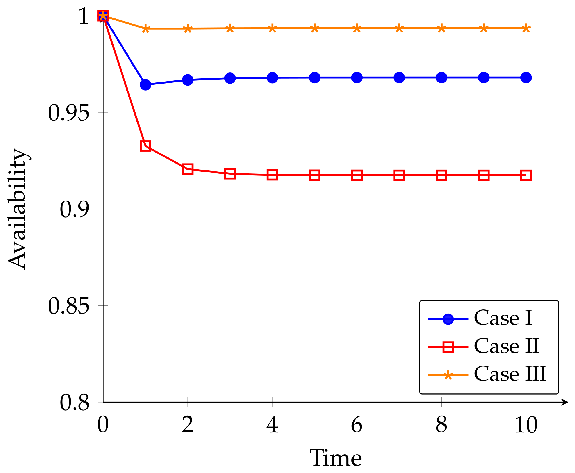
The three availability scenarios allow a full assessment of the design and operational strategies that engineers and maintenance managers can utilize to improve system reliability. Insights beyond the specific case outcomes are provided jointly by

Table 3. Availability measures in transient and steady-state over the time interval t ∈ [0, 10] for three repair scenarios: Gumbel–Hougaard copula repair (Case I), general distribution repair (Case II) and component quality degradation method at $\rho$ = 0.2 (Case III).

Time	Case I	Case II	Case III
0	1	1	1
1	0.964279	0.932569	0.993327
2	0.966726	0.920631	0.993335
3	0.967672	0.918204	0.993466
4	0.967888	0.917636	0.993519
5	0.967937	0.917489	0.993537
6	0.967949	0.91745	0.993544
7	0.967952	0.917439	0.993546
8	0.967954	0.917437	0.993547
9	0.967954	0.917437	0.993547
10	0.967954	0.917437	0.993547

and Figure 3.

Steady-state hierarchy interpretation. The steady-state availability ranking, Case III (99.35 %) > Case I (96.80 %) > Case II (91.74 %) illustrates a significant difference between two reliability improvement techniques: proactive failure avoidance and reactive repair optimization. Case III is the dominant case because it directly reduces the failure rates (and hence the probability of entering any failed or degraded state), while Cases I and II are only reducing the rate of recovery from such states once they have been attained. The 5.06% point difference between Cases I and II precisely measures the benefit of dependent repair modeling via copula over independence-based general repair as the extra availability that can be recovered through coordinated maintenance without changing the quality of components or the system architecture.

Practical design considerations: The three-case analysis shows a clear hierarchy of the effectiveness of interventions. Finally, when the maximum system availability is the first goal, the proactive improvement of the quality of the components (Case III) must be the first choice, since it increases the steady-state availability limit and also reduces the frequency of all failure events that have repair costs. Copula-based repair modeling (Case I) offers substantial benefits over naive general repair (Case II), particularly when the opportunity for proactive quality improvement is limited by cost or supply chain constraints. This demonstrates that the choice of a repair dependence model is not merely a mathematical refinement but has tangible operational consequences. A synergistic approach, quality improvement plus coordinated copula-structured maintenance, should result in availability levels at or above Case III, while enjoying the repair efficiency benefits identified in the Case I versus Case II analysis.

Sensitivity to attenuation factor $\rho$. The conclusion of Case III is limited to $\rho =0.2$. The effect of the choice of $\rho$ on the steady-state availability is an important factor in the cost-benefit analysis: as $\rho$ decreases to zero, all failure rates go to zero and the availability goes to one, but the cost of achieving sufficiently small failure rates by investing in component quality increases nonlinearly. The relationship between the reduction factor, the resulting availability gain and the procurement cost difference is a natural extension of the present analysis to a jointly optimized quality maintenance decision framework as a possible research direction in Section 5.

4.2. System Reliability Analysis and Evaluation

Reliability is different in concept from availability in that reliability is a measure of the probability of continuous operation without failure for a specified period of time and does not permit repairs once a fault has occurred. The reliability function $R(t)$ is defined as the probability that the system has not experienced a complete failure by time t, given that it was fully functional at t = 0. This statistic is particularly important for mission-critical applications where the system is required to operate continuously for a certain period of time, e.g., continuous monitoring on a factory floor during a production shift, where repair actions cannot be initiated while the mission is in progress.

The reliability function is obtained from Equation (49) by setting all the repair rates equal to zero, i.e., neglecting all the return transitions from the failed and degraded states to the functioning state $S_0$. Under this no repair assumption, the probability mass of each failed state is irretrievably lost, while the surviving probability is redistributed only to the remaining operating and degraded states. Then, we take the inverse Laplace transform to obtain $R(t)$ in the time domain. Two cases are analyzed with different levels of used component failure rates.

Case I: Reliability Under Baseline Failure Rates

For the first reliability scenario, the same baseline failure rate parameters defined in Section 4.1 are used. These values are for the system at nominal component quality conditions with no proactive failure rate reduction. Setting all repair rates to zero in Equation (49) and applying the inverse Laplace transform yields the time-domain reliability function:

$$\begin{array}{c}R(t)=-0.579759e^{-0.72t}+0.731707e^{-0.31t}+0.163043e^{-0.26t}+0.0000735294e^{-0.21t}\hfill \\ +0.574074e^{-0.18t}+0.0315789e^{-0.15t}+0.0331034e^{-0.14t}\\ \hfill +0.0027e^{-0.12t}+0.0434783e^{-0.03t}\end{array}$$

(54)

Case II: Reliability Under Reduced Failure Rates

The second reliability scenario is the component quality reduction approach with the reduction factor $\rho$ = 0.2, which reduced all baseline failure rates to 20% of the nominal ones. This scenario still entails a significant reduction in failure rates (to 20% of baseline) but still keeps the contrast between Cases I and II analytically pedagogical. Substituting these reduced parameters into Equation (49) with all repair rates set to zero and applying the inverse Laplace transform yields

$$\begin{array}{c}R(t)=-0.394913e^{-0.144t}+0.731707e^{-0.062t}+0.0326087e^{-0.052t}+1.17647({10}^{-7})e^{-0.042t}\\ +0.574074e^{-0.036t}+0.00631579e^{-0.03t}+0.00662069e^{-0.028t}\\ +0.000108e^{-0.024t}+0.0434783e^{-0.006t}\end{array}$$

(55)

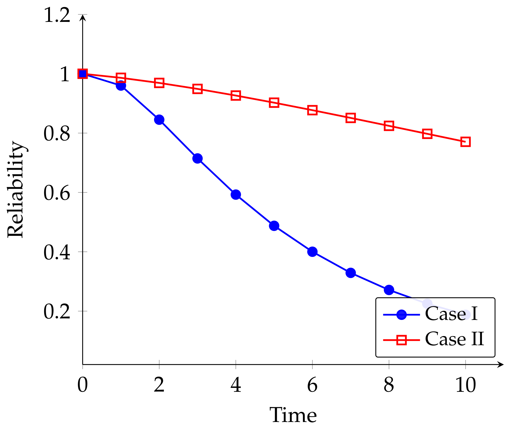
The most remarkable property that can be observed in

Table 4. Time-dependent system reliability for t ∈ [0, 10] under the baseline failure rate configuration (Case I) and the lowered failure rate configuration at $\rho$ = 0.2 (Case II), assessed using a no-repair assumption.

Time	Case I	Case II
0	1	1
1	0.960298	0.986391
2	0.845239	0.969137
3	0.714663	0.949002
4	0.592764	0.926633
5	0.487583	0.902575
6	0.400192	0.877288
7	0.328947	0.851158
8	0.271393	0.824508
9	0.225062	0.797604
10	0.187775	0.77067

and Figure 4 is the concavity of the Case I curve. The biggest decline is between t = 0 and t = 3; then, the decline rate slowed down as the major fast decaying factors mostly disappeared. The curve for Case II, on the other hand, is still almost linear over the shown range t ∈ [0, 10] in Figure 4, with a slow and almost uniform rate of decrease similar to the slow decay rates of the dominant terms in Equation (55). The steep concave decline versus the almost linear slow decline visually summarizes the fundamental reliability change that can be achieved by investing in component quality and makes Figure 4 one of the best communication outputs in the study.

4.3. Analysis of Mean Time to Failure $MTTF$

The mean time to failure ($MTTF$) is the anticipated period from when the system becomes fully operational to its initial complete failure, assuming no repairs are conducted. It offers a singular scalar summary of system longevity that enhances the time-dependent reliability curves of Section 4.2 and serves as a fundamental basis for analyzing the relative impact of individual failure rate parameters on total system lifespan. Mathematically, the mean time to failure ($MTTF$) is determined by calculating the limit of the Laplace transform of $P_{up}(s)$ as s → 0, with all repair rates set to zero:

$$MTTF=\underset{s\to 0}{lim}{\stackrel{*}{P}}_{up}(s)$$

Applying this constraint to the five-subsystem model established in Section 3 and simplifying results in the closed-form expression:

$$\begin{array}{c}MTTF={\displaystyle \frac{1}{{\alpha }_1+5{\alpha }_2+4{\alpha }_3+6{\alpha }_4+{\alpha }_5+{\alpha }_6+{\alpha }_7}}[2+4{\alpha }_3\left({\displaystyle \frac{3{\alpha }_3}{2{\alpha }_3+{\alpha }_6+{\alpha }_7}}+{\displaystyle \frac{1}{3{\alpha }_3+{\alpha }_6+{\alpha }_7}}\right)\hfill \\ +6{\alpha }_4\left({\displaystyle \frac{5{\alpha }_4}{4{\alpha }_4+{\alpha }_6+{\alpha }_7}}+{\displaystyle \frac{20{\alpha }_4^4}{3{\alpha }_4+{\alpha }_6+{\alpha }_7}}+{\displaystyle \frac{1}{5{\alpha }_4+{\alpha }_6+{\alpha }_7}}\right)\\ \hfill +5{\alpha }_2\left({\displaystyle \frac{1}{4{\alpha }_2+{\alpha }_6+{\alpha }_7}}+4{\alpha }_2\left({\displaystyle \frac{3{\alpha }_2}{2{\alpha }_2+{\alpha }_6+{\alpha }_7}}+{\displaystyle \frac{1}{3{\alpha }_2+{\alpha }_6+{\alpha }_7}}\right)\right)]\end{array}$$

(56)

The analytical form of Equation (56) is quite revealing. The main denominator factor, the sum of all effective failure rates multiplied by their respective unit multiplicities, is the total instantaneous rate of decrease in the fully operational state, $S_0$. The numerator in brackets is the redundancy advantage of each k-out-of-n subsystem that is always larger than one and represents the additional expected operational lifetime of the degraded-but-operational states prior to the system failure. Subsystems with high unit numbers and low k thresholds contribute more significantly to the numerator, consistent with the reasoning that greater redundancy leads to longer system lifetimes. The environmental failure rates ${\alpha }_6$ and ${\alpha }_7$ appear both in the denominator and inside fractions in the numerator. They are the competing stressors that simultaneously accelerate the deviation from $S_0$ and decrease the mean sojourn lengths in degraded states.

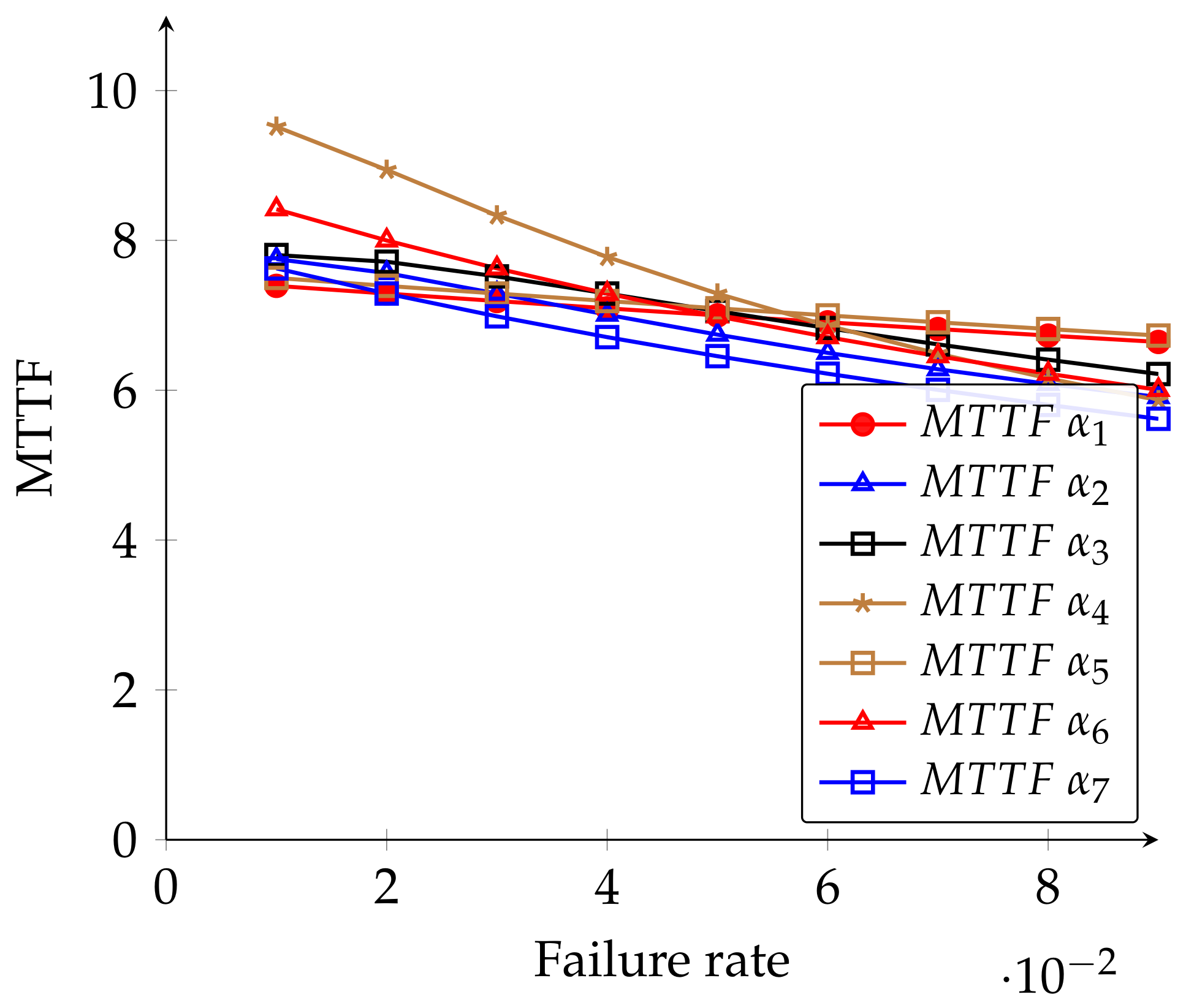
The $MTTF$ values of the seven parameters at nine different failure rates from 0.01 to 0.09 are given in

Table 5. Mean time to failure ($MTTF$) as a function of individual subsystem failure rates ${\alpha }_1$ through ${\alpha }_7$, varied independently over the interval [0.01, 0.09] while all remaining parameters are held at their baseline values.

Failure Rates	$\mathit{MTTF}$ (${\mathit{\alpha }}_1$)	$\mathit{MTTF}$ (${\mathit{\alpha }}_2$)	$\mathit{MTTF}$ (${\mathit{\alpha }}_3$)	$\mathit{MTTF}$ (${\mathit{\alpha }}_4$)	$\mathit{MTTF}$ (${\mathit{\alpha }}_5$)	$\mathit{MTTF}$ (${\mathit{\alpha }}_6$)	$\mathit{MTTF}$ (${\mathit{\alpha }}_7$)
0.01	7.39331	7.75062	7.80443	9.51733	7.49892	8.41585	7.62635
0.02	7.29062	7.56443	7.71544	8.94182	7.39331	7.99906	7.29062
0.03	7.19075	7.29062	7.51943	8.33338	7.29062	7.62635	6.98629
0.04	7.09358	7.00872	7.29062	7.77908	7.19075	7.29062	6.70887
0.05	6.999	6.74259	7.05671	7.29062	7.09358	6.98629	6.45475
0.06	6.9069	6.49933	6.82902	6.86315	6.999	6.70887	6.22094
0.07	6.8172	6.2801	6.61221	6.48852	6.9069	6.45475	6.00496
0.08	6.7298	6.08386	6.40792	6.1588	6.8172	6.22094	5.80475
0.09	6.64462	5.90882	6.21644	5.86709	6.7298	6.00496	5.61855

. From any row in Table 4 it can be seen that the parameters have a hierarchical influence at the given failure rate, and the ranking is stable for all rows: ${\alpha }_4$ always leads to the smallest $MTTF$, followed by ${\alpha }_6$, ${\alpha }_7$, ${\alpha }_2$, ${\alpha }_3$, ${\alpha }_5$, and ${\alpha }_1$ in approximately this order. The consistent ranking through the whole evaluation range confirms that the sensitivity ordering is a property of the system architecture and not an effect of the specific baseline parameter values used.

Figure 5 converts these tabular numbers into a graphic representation that clearly highlights three aspects. The ${\alpha }_7$ curve is always below all the others for the entire range of failure rates, and its slope is steeper, which makes it deviate more from the other curves as the failure rate increases, confirming that SS4 is the main reliability constraint of the system. The curves of ${\alpha }_6$ and ${\alpha }_7$ also drop more steeply than those of ${\alpha }_1$, ${\alpha }_3$, and ${\alpha }_5$, but less than ${\alpha }_4$, so they fall in an intermediate range of their own, indicating their systemic environmental effect. The ${\alpha }_1$ and ${\alpha }_5$ curves are very consistent throughout the image, visually confirming their very similar sensitivity profiles.

Collectively, Table 5 and Figure 5 provide a systematic approach to improving reliability investments: improvements to mitigate ${\alpha }_4$ through better photovoltaic modules, better vibration isolation mounting, or more robust thermal control of the power subsystem will lead to the highest per-unit increase in system $MTTF$. The second most cost-effective intervention is environmental control techniques that reduce both ${\alpha }_6$ and ${\alpha }_7$ simultaneously, especially when the benefits from these techniques diffuse across all five subsystems instead of only one.

4.4. Sensitivity Study of the Mean Time to Failure $MTTF$

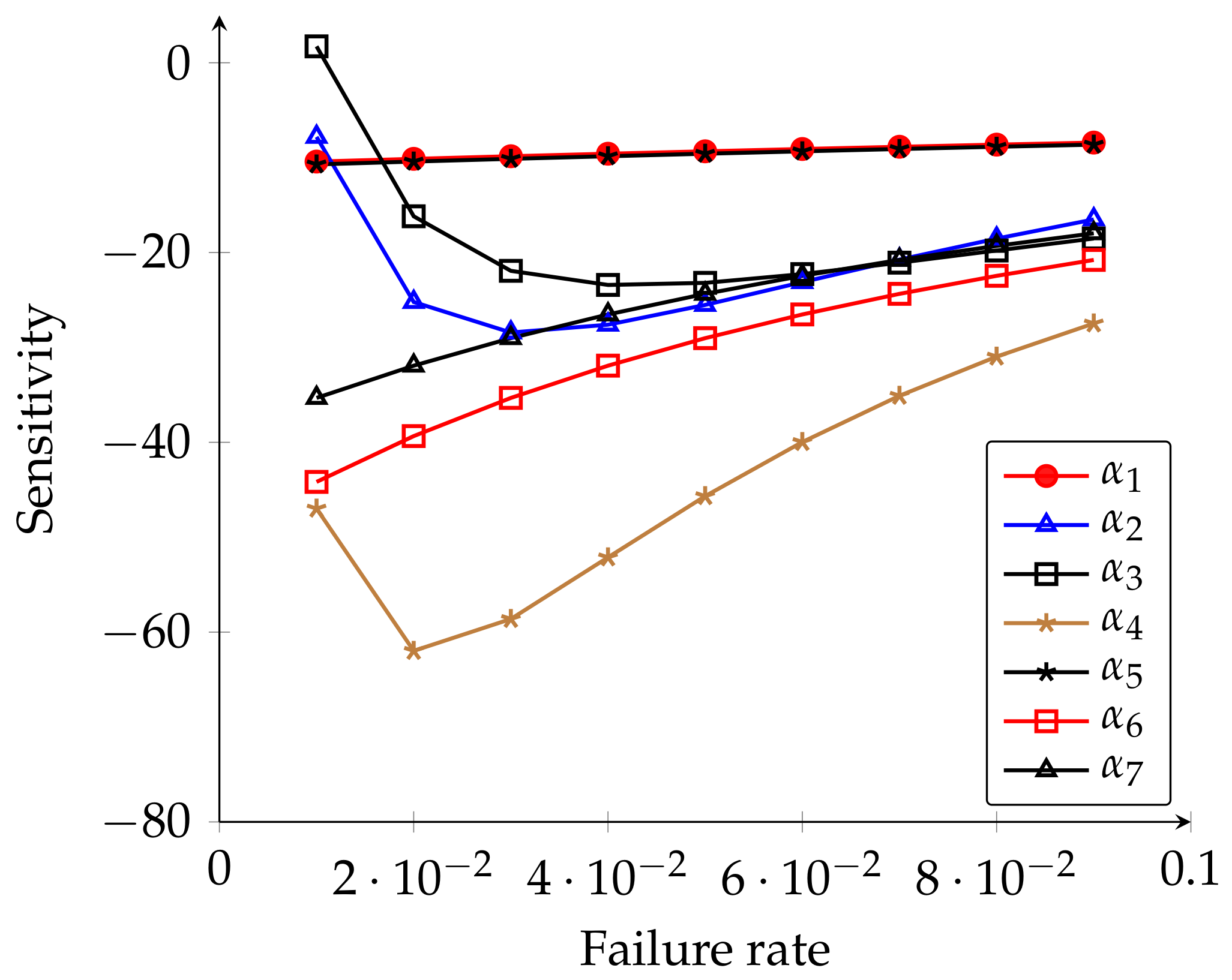
Sensitivity analysis provides a more precise and locally exact characterization of these relationships by computing the partial derivative of $MTTF$ with respect to each failure rate parameter at the baseline operating point. Formally, the sensitivity index with respect to parameter ${\alpha }_i$ is defined as ∂($MTTF$)/∂${\alpha }_i$

This variable quantifies the instantaneous rate of change of $MTTF$ with respect to a unit increase in ${\alpha }_i$, assessed at the baseline parameter values. A significant negative value of $S_i$ signifies that $MTTF$ is acutely responsive to ${\alpha }_i$, indicating that a minor increase in that failure rate results in a disproportionately substantial decrease in anticipated system longevity, thereby designating ${\alpha }_i$ as a critical focus for reliability enhancement initiatives. In contrast, a minor negative value signifies that ${\alpha }_i$ exerts minimal marginal impact on $MTTF$ at the present operating point, indicating that efforts to mitigate it will produce very modest benefits. As shown in Section 4.3, $MTTF$ is always decreasing with respect to each failure rate parameter. We see that the sign of ∂($MTTF$)/∂${\alpha }_3$ changes at the lower end of the range studied, being negative for  ${\alpha }_3$⩾ 0.02 and negative afterward. This is because for very small ${\alpha }_3$, the redundancy benefit terms in the $MTTF$ expression (Equation (56)) associated with SS3 (2-out-of-4) are still increasing with ${\alpha }_3$ faster than the denominator’s departure-rate effect, giving a short net positive marginal effect before the failure rate penalty kicks in for ${\alpha }_3\ge 0.02$. The partial derivatives are obtained by differentiating Equation (56) analytically with respect to each ${\alpha }_i$ and substituting the baseline values: ${\alpha }_1=0.02,{\alpha }_2=0.03,{\alpha }_3=0.04,{\alpha }_4=0.05,{\alpha }_5=0.03,{\alpha }_6=0.04,{\alpha }_7=0.02$. The sensitivity indices are calculated by varying each ${\alpha }_i$ individually in the interval [0.01, 0.09] while keeping the other parameters at their baseline values. The complete set of sensitivity values are shown in

Table 6. Partial derivative sensitivity indices ∂($MTTF$)/∂${\alpha }_i$ for each failure rate parameter ${\alpha }_i$, i = 1, …, 7, calculated over the range [0.01, 0.09], measuring the marginal effect of each failure rate on the system mean time to failure.

Failure Rates	$\frac{\mathit{\partial }(\mathit{MTTF})}{\mathit{\partial }{\mathit{\alpha }}_1}$	$\frac{\mathit{\partial }(\mathit{MTTF})}{\mathit{\partial }{\mathit{\alpha }}_2}$	$\frac{\mathit{\partial }(\mathit{MTTF})}{\mathit{\partial }{\mathit{\alpha }}_3}$	$\frac{\mathit{\partial }(\mathit{MTTF})}{\mathit{\partial }{\mathit{\alpha }}_4}$	$\frac{\mathit{\partial }(\mathit{MTTF})}{\mathit{\partial }{\mathit{\alpha }}_5}$	$\frac{\mathit{\partial }(\mathit{MTTF})}{\mathit{\partial }{\mathit{\alpha }}_6}$	$\frac{\mathit{\partial }(\mathit{MTTF})}{\mathit{\partial }{\mathit{\alpha }}_7}$
0.01	−10.4131	−7.81155	1.72816	−46.9831	−10.7127	−44.1679	−35.3178
0.02	−10.1259	−25.212	−16.1798	−61.9727	−10.4131	−39.3417	−31.9204
0.03	−9.85034	−28.429	−21.928	−58.6125	−10.1259	−35.3178	−29.0207
0.04	−9.58592	−27.6026	−23.4127	−52.1204	−9.85034	−31.9204	−26.5223
0.05	−9.33199	−25.5196	−23.1953	−45.6691	−9.58592	−29.0207	−24.3517
0.06	−9.08803	−23.1187	−22.2701	−39.9661	−9.33199	−26.5223	−22.4517
0.07	−8.85351	−20.7466	−21.0674	−35.0929	−9.08803	−24.3517	−20.7777
0.08	−8.62795	−18.5307	−19.7856	−30.9663	−8.85351	−22.4517	−19.2938
0.09	−8.41091	−16.5107	−18.5184	−27.4706	−8.62795	−20.7777	−17.9714

and visualized in Figure 6.

4.5. Cost Analysis

The real operational value of a repairable system is determined by its technical reliability measures and also by its economic performance over time. In this section, the expected profit of the system in the interval [0, t] is evaluated taking into consideration the revenue due to successful operation and the costs due to maintenance and repair activities. The expected profit function is defined as

$$E_p(t)=C_1{\int }_0^t{P}_{up}(\tau )d\tau -C_{2}t$$

(57)

where $C_1$ represents the revenue rate earned per unit time that the system is operational, and $C_2$ represents the total maintenance and service expenditure rate per unit time, which is presumed to be constant and continuous regardless of the system’s state. This integration denotes the revenue-generating premise, which is the cumulative expected operational time over the interval [0, t]. The net expected profit is determined by the difference between revenue and cost. This profit may be positive or negative depending on the balance between the availability of the system and the costs of maintenance.

Case I: Expected Profit Under Gumbel–Hougaard Copula Repair

Substituting the availability expression from Equation (51) into Equation (57) and evaluating the integral analytically using the parameter values established in Case I of Section 4.1 yields the expected profit function:

$$\begin{array}{cc}\hfill E_p(t)=& (0.000525794-0.0247618e^{-2.95038t}+0.022281e^{-1.74588t}+0.000355853e^{-1.27216t}\hfill \\ & +0.00023372e^{-1.21308t}+0.000128643e^{-1.14395t}+0.000646094e^{-1.09033t}-5.41296({10}^{-6})e^{-1.02815t}\hfill \\ & +0.000245175e^{-0.951733t}+0.000351017e^{-0.841796t}-3.90318({10}^{-12})e^{-0.31t}+9.06256({10}^{-11})e^{-0.21t}\hfill \\ & -2.1098({10}^{-10})e^{-0.18t}+3.63241({10}^{-10})e^{-0.15t}-2.67489({10}^{-10})e^{-0.14t}+2.29133({10}^{-11})e^{-0.12t}\hfill \\ & \hfill +2.76549({10}^{-14})e^{-0.03t}+0.967954t)C_1-C_{2}t\end{array}$$

(58)

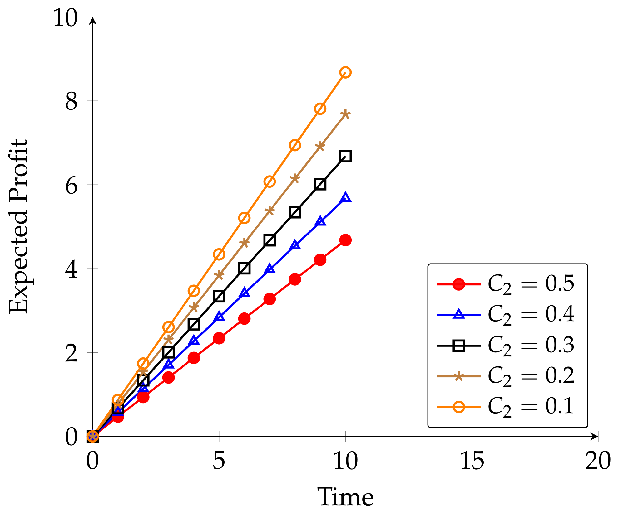
This is possible if $C_2$ < 0.967954 $C_1$ and the system will be viable in the long term if it is positive. The fact that all five maintenance cost levels ($C_2=0.1$ to $0.5$) satisfy this condition with $C_1=1$ is a confirmation that the copula repair strategy is profitable in the long run for the entire range of maintenance costs considered. This is the case for the parameter values considered in

Table 7. Expected system profit $E_p(t)$ over t ∈ [0, 10] under Gumbel–Hougaard copula repair (Case I), computed for five maintenance cost levels $C_2$∈ {0.1, 0.2, 0.3, 0.4, 0.5} with fixed revenue rate $C_1$ = 1.

Time	${\mathit{C}}_2=0.5$	${\mathit{C}}_2=0.4$	${\mathit{C}}_2=0.3$	${\mathit{C}}_2=0.2$	${\mathit{C}}_2=0.1$
0	0	0	0	0	0
1	0.471744	0.571744	0.671744	0.771744	0.871744
2	0.937281	1.13728	1.33728	1.53728	1.73728
3	1.40459	1.70459	2.00459	2.30459	2.60459
4	1.87239	2.27239	2.67239	3.07239	3.47239
5	2.34031	2.84031	3.34031	3.84031	4.34031
6	2.80826	3.40826	4.00826	4.60826	5.20826
7	3.27621	3.97621	4.67621	5.37621	6.07621
8	3.74416	4.54416	5.34416	6.14416	6.94416
9	4.21211	5.11211	6.01211	6.91211	7.81211
10	4.68007	5.68007	6.68007	7.68007	8.68007

. Thus, for long periods, the profit curves in Figure 7 are totally parallel straight lines. The lines are separated by a vertical gap between any two cost levels that grows linearly with t and is equal to $\Delta$$C_2$ × t.

Case II: Expected Profit Under General Distribution Repair

Substituting the availability expression from Equation (52) into Equation (57) under the general repair scenario yields

$$\begin{array}{c}{E}_p(t)=(0.0491653-0.0322957e^{-1.94909t}-0.00173725e^{-1.27567t}-0.00148829e^{-1.21573t}\hfill \\ -0.00181317e^{-1.14625t}-0.00896669e^{-1.10362t}+0.000593732e^{-1.02769t}-0.00964006e^{-1.01455t}\\ +0.00338288e^{-0.946967t}+0.00279921e^{-0.839589t}+1.97429({10}^{-11})e^{-0.31t}-1.9752({10}^{-11})e^{-0.21t}\\ -3.96268({10}^{-11})e^{-0.18t}+1.84879({10}^{-10})e^{-0.15t}-1.61485({10}^{-10})e^{-0.14t}+1.87584({10}^{-11})e^{-0.12t}\\ \hfill +2.08493({10}^{-14})e^{-0.03t}+0.917437t)C_1-C_{2}t\end{array}$$

(59)

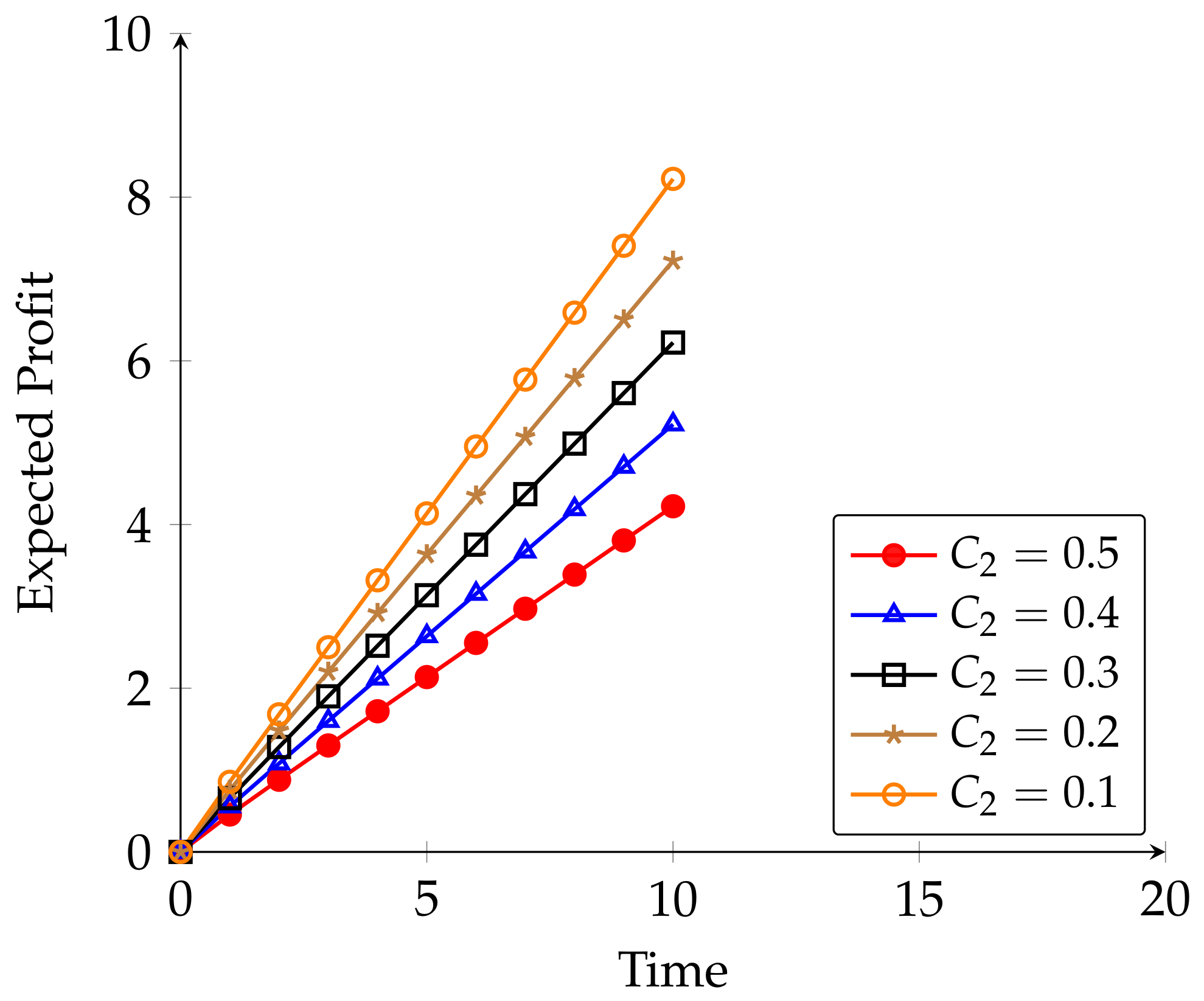
Compared directly with Case I, the general repair case gives an asymptotic profit rate that is smaller by 0.050517 $C_1$ per unit time. When $t=10$, $C_1=1$, and $C_2=0.2$, the cumulative profit shortfall with respect to Case I is 0.505 time units of revenue. We can check this by looking at Figure 8 and

Table 8. Expected system profit $E_p(t)$ over t ∈ [0, 10] under general distribution repair (Case II), computed for five maintenance cost levels $C_2$∈ {0.1, 0.2, 0.3, 0.4, 0.5} with fixed revenue rate $C_1$ = 1.

Time	${\mathit{C}}_2=0.5$	${\mathit{C}}_2=0.4$	${\mathit{C}}_2=0.3$	${\mathit{C}}_2=0.2$	${\mathit{C}}_2=0.1$
0	0	0	0	0	0
1	0.456765	0.556765	0.656765	0.756765	0.856765
2	0.881788	1.08179	1.28179	1.48179	1.68179
3	1.30091	1.60091	1.90091	2.20091	2.50091
4	1.71877	2.11877	2.51877	2.91877	3.31877
5	2.13631	2.63631	3.13631	3.63631	4.13631
6	2.55378	3.15378	3.75378	4.35378	4.95378
7	2.97122	3.67122	4.37122	5.07122	5.77122
8	3.38866	4.18866	4.98866	5.78866	6.58866
9	3.8061	4.7061	5.6061	6.5061	7.4061
10	4.22354	5.22354	6.22354	7.22354	8.22354

and comparing the relevant entries. As time goes on, the difference in profits keeps growing without bound. This means that the copula based dependent repair is not only a better way to do general independent repair for a short duration of time in terms of money, it is a long-term benefit that keeps growing as long as the system is functioning. Without the positive reliance structure provided by the copula, units that fail together require a longer time to recover together and hence delay the return to full revenue-generating capacity following initial failure events. The values of profit for Case II are given in Table 8 and are shown in Figure 8. The inferior trend in all levels of maintenance cost compared to Case I is evidently clear.

Case III: Expected Profit Under the Component Quality Reduction Technique

The availability expression from Equation (53) is substituted into Equation (57) with the reduction approach with $\rho$ = 0.2, giving

$$\begin{array}{c}{E}_p(t)=(0.00086851-0.00284986e^{-2.7398t}+0.00105044e^{-1.15127t}-0.0000179379e^{-1.05497t}\hfill \\ +0.000273009e^{-1.03653t}-0.0267054e^{-1.02027t}+0.0277647e^{-1.01997t}-0.000470593e^{-1.00744t}\\ +0.0000644717e^{-0.990117t}+0.0000226928e^{-0.96639t}-3.38404({10}^{-12})e^{-0.062t}+4.5652({10}^{-11})e^{-0.052t}\\ -2.87879({10}^{-10})e^{-0.042t}+6.09876({10}^{-10})e^{-0.036t}-1.06318({10}^{-9})e^{-0.03t}+7.53275({10}^{-10})e^{-0.028t}\\ \hfill -6.12215({10}^{-11})e^{-0.024t}-5.50946({10}^{-13})e^{-0.006t}+0.993547t)C_1-C_{2}t\end{array}$$

(60)

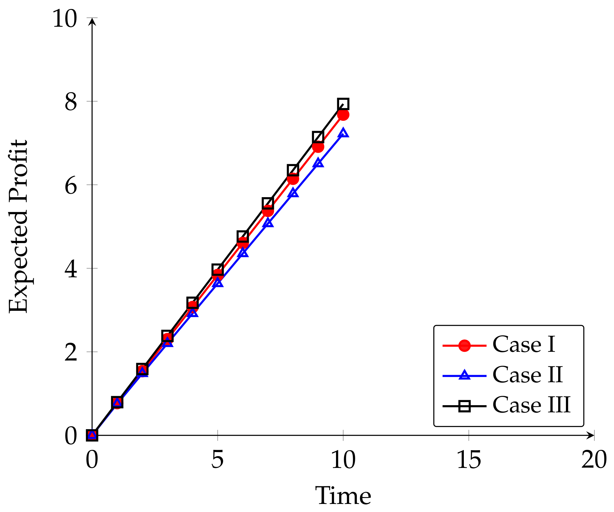
This represents the maximum asymptotic profit rate across all three cases, surpassing Case I by 0.025593 $C_1$ per unit time and Case II by 0.076110 $C_1$ per unit time. At t = 10, with $C_1$ = 1 and $C_2$ = 0.2, the cumulative projected profit in Case III attains 7.936, in contrast to 7.680 in Case I and 7.224 in Case II—hence substantiating the profit hierarchy of Case III > Case I > Case II across all time points and maintenance costs analyzed.

A direct three-way comparison of expected profit at $C_2$ = 0.2 across all three cases over t ∈ [0, 10] is presented in

Table 9. The comparative expected profit $E_p(t)$ of the system in the interval $t\in [0,10]$ with a constant maintenance cost $C_2$ = 0.2 under three scenarios: Gumbel–Hougaard copula repair (Case I), general distribution repair (Case II), reduction method for component quality at $\rho$ = 0.2 (Case III).

Time	Origin (${\mathit{C}}_2$ = 0.2)	General (${\mathit{C}}_2$ = 0.2)	$\mathit{\rho }=0.2$ (${\mathit{C}}_2$ = 0.2)
0	0	0	0
1	0.771744	0.756765	0.7949
2	1.53728	1.48179	1.58818
3	2.30459	2.20091	2.38159
4	3.07239	2.91877	3.17508
5	3.84031	3.63631	3.96861
6	4.60826	4.35378	4.76215
7	5.37621	5.07122	5.5557
8	6.14416	5.78866	6.34925
9	6.91211	6.5061	7.14279
10	7.68007	7.22354	7.93634

. The hierarchy is not a transient artifact, but a structural property of the steady-state availability differences between the three scenarios, as evidenced by the fact that the profit ranking Case III > Case I > Case II is established immediately at t = 1 and maintained at every subsequent time step without exception. Figure 9 depicts this comparison with three upward-sloping profit lines emanating from a common point at t = 0 and diverging from each other. Case III exhibits the fastest rise, Case I the intermediate slope and Case II the slowest. All of them attain their asymptotic values by t ≈ 3. The three lines are visually distinguished by their slopes throughout the figure. This simple visual message perhaps represents the most practically communicable result of the entire paper, translating a complex stochastic reliability model into a directly actionable financial argument for component quality investment in smart factory monitoring systems. This message indicates that Case III has a higher revenue-side profit rate than Cases I and II under the maintenance cost structure considered in this study. This result should be interpreted as isolating the availability benefit of the failure rate reduction, rather than a complete economic comparison inclusive of the quality-investment cost.

5. Conclusions

5.1. Summary of Methodology

The present paper deals with a detailed reliability analysis of a five-subsystem hybrid series-parallel system to model the smart factory monitoring infrastructure working under severe thermal and mechanical conditions. The system consists of different k-out-of-n redundancy systems, i.e., a central PLC (1-out-of-1), pressure and temperature sensors (2-out-of-5), wireless communication units (2-out-of-4), solar power modules (3-out-of-6), and a cold standby database server (1-out-of-2), which indicates the differing criticality of subsystems.

The present study is distinguished by three methodological innovations that differentiate it from previous work. The model statistically characterizes dependent repair durations between units that fail simultaneously using the Gumbel–Hougaard copula family, instead of the independence assumption that is typical of current multi-subsystem models. Second, the combination of cold standby redundancy in subsystem five with copula-based repair is presented in a unified analytical framework, which is not found in previous studies. Third, environmental failure is decomposed into two separate stressors, thermal stress (${\alpha }_6$) and vibrational stress (${\alpha }_7$), rather than being lumped into a single environmental parameter, which permits more accurate mitigation.

Three analytical cases were considered: Case I with Gumbel–Hougaard copula repair, Case II with general distribution repair and Case III with a component quality reduction technique controlled by factor $\rho$. Closed-form expressions of system availability, reliability, mean time to failure ($MTTF$), sensitivity indices and expected profit were obtained using Laplace transforms and supplementary variable techniques.

5.2. The Numerical Findings Yield Numerous Important Insights

• Availability. The steady state availability is 96.80% for copula-based repair (Case I), 91.74% for general repair (Case II) and 99.35% for the reduction technique (Case III, $\rho$ = 0.2). The significantly improved availability in Case III shows that the best way to ensure continued system performance is to proactively reduce component failure rates by improving manufacturing quality or enhancing environmental protection.
• Reliability. The time dependent reliability study shows that reducing the failure rate by a factor of $\rho$ = 0.2 (Case II of the reliability analysis) significantly increases the time the system maintains exceptional reliability. At t = 10, the dependability achieved with the reduction strategy (77.07%) is almost four times better than that of the baseline instance (18.78%), showing the long-term benefits of investing in component quality.
• Mean Time To Failure and Sensitivity. According to the $MTTF$ study, the subsystem SS4 (solar power modules, ${\alpha }_4$) and the environmental parameters (${\alpha }_6$ and ${\alpha }_7$) are the ones that have the most negative effect on the system life expectancy. The partial derivative ∂($MTTF$)/∂${\alpha }_4$ reaches −45.6691 at the baseline failure rate, indicating that SS4 is the dominant subsystem for reliability improvement effort. The failure rates of the PLC (${\alpha }_1$) and the SS5 standby unit (${\alpha }_5$) are not very sensitive, indicating the protective effect of redundancy in these subsystems.
• The Expected Profit. The cost analysis indicated that all three scenarios projected a profit over the evaluated period, with the reduction method (Case III) yielding the highest cumulative profit. The economic case for preventative maintenance over reactive repair is supported by maintenance expenditure rates ($C_2$) that are consistently lower, boosting profit margins in all cases.

The proposed method provides a flexible and analytically sound framework for assessing the reliability of complex industrial monitoring systems. The integration of copula-based dependent repair modeling, dual environmental failure rates and cold standby redundancy is a significant improvement, compared with the existing single-parameter or independence-assumption models. Future research may consider non-exponential failure probabilities of single units, multi-state degradation models or the optimization of the maintenance scheduling inside the copula-repair framework to bridge the gap between theoretical modeling and real-world industrial requirements.

5.3. Practical Implications

The results of this study are of great practical importance to engineers, maintenance planners, and decision makers involved in running smart factory monitoring systems in thermally and mechanically demanding environments.

• Subsystems prioritization for maintenance allocation. From the sensitivity analysis, the subsystem SS4 (3-out-of-6 solar power modules) has the most negative impact on $MTTF$. The sensitivity value is −45.6691 at the baseline failure rates. This score identifies SS4 as the leading candidate for increased protective measures such as vibration dampening mounts, thermal shielding, or more frequent inspections. This subsystem should be prioritized in maintenance budgets over other subsystems.
• Environmental monitoring is also an operational necessity, in parallel. It is of immediate operational importance to separate environmental failure into thermal stress (${\alpha }_6$) and vibrational stress (${\alpha }_7$) as independent entities instead of a single aggregate. Facilities can deploy autonomous heat and vibration monitoring sensors, each with its own alarm threshold, allowing for precise corrective actions. A heat exceedance event does not necessarily mean termination of vibration-sensitive components and vice versa. Such granularity minimizes unnecessary downtime and allows more precise root cause analysis when failure events do occur.
• Cost-effective cold standby redundancy: A strategy for enhancing the resilience of critical data infrastructure. The 1-out-of-2 cold standby scheme in SS5 (the database server) shows that the most data-critical component of the system can be effectively protected by keeping an inactive backup unit, with no failure rate while on standby. Professionals who design industrial IoT or SCADA systems must plan for cold standby arrangements, especially for database and logging servers where data integrity is critical, and the cost of a backup unit is negligible compared to the cost of data loss or unexpected outages.
• Quality improvements in the components surpass remedial fixes. The reduction method (Case III, $\rho$ = 0.2) yields the highest steady-state availability (99.35%) and the largest expected profit among the three cases. This implies that a high-quality component (with a lower failure rate) has a higher long-term advantage than an efficient repair procedure. This result provides procurement teams a numerical justification to opt for higher-quality sensors, communication units, and power modules instead of the cheaper alternatives, especially in environments subjected to significant thermal or seismic stress.
• Copula-based repair modeling for pragmatic maintenance planning. The Gumbel–Hougaard copula approach addresses a practical problem which is often ignored in traditional models, i.e., the repair times of multiple unit failures are rarely independent. Standardized spare parts, coordinated environmental restoration, and collaborative maintenance teams establish a mutually beneficial interdependence in terms of repair times. Maintenance schedulers can use these data to optimize staff deployment and spare parts inventory for linked failure scenarios, rather than relying on isolated repair queues in worst-case scenarios, allowing for more accurate downtime predictions and improved efficiency in resource allocation.
• Anticipated profits for the purpose of assisting in decision-making. The cost analysis method, symbolized by Equation (57), is a useful tool which can be employed by operations managers. The expressions for expected profit given in Equations (58)–(60) can be useful for negotiating contracts, designing service level agreements and pricing insurance for industrial monitoring systems. This is done by tuning $C_1$ (revenue per unit time of operation) and $C_2$ (maintenance cost per unit time) for site-specific financial considerations.

5.4. Limitations and Future Work

Limitations: The scope of the present results is limited by several modeling assumptions, which should be considered when interpreting or applying them. To begin, we assume that the failure of each unit can be modeled as an exponential distribution with a constant rate; this memoryless assumption, although analytically tractable and a standard one in this literature, does not account for wear-out or aging effects that many physical components (e.g., photovoltaic modules, sensors under thermal cycling) experience as a function of their operational lifetime. Second, the two environmental failure rates (${\alpha }_6$, ${\alpha }_7$) are assumed to be constant and independent of each other; in practice, thermal and vibrational stress levels often vary seasonally or diurnally and may be correlated with each other and with operational load. Third, the Gumbel–Hougaard copula parameter and the general repair distributions are specified from representative baseline values rather than estimated from field failure/repair data, because no such dataset was available for this system. The qualitative conclusions (e.g., the availability hierarchy across the three cases) are expected to be robust to this choice, but the precise numerical values reported would shift under different parameterizations. Fourth, the component quality reduction technique (Case III) is considered for a single reduction factor ($\rho =0.2$) without a cost model to achieve that reduction, noting the cost of achieving the failure rate reduction $\rho$ (e.g., higher-grade components, tighter manufacturing tolerances). A fair economic comparison of proactive quality investment with reactive repair strategies would necessitate an explicit quality-investment cost function, which we identify as a natural and important direction for future work. Finally, the model assumes perfect, as-good-as-new restoration after repair of any fully failed state, which may not be true for components which are subject to partial degradation after repair.

Future Work: Based on these limitations, future research directions include multi-objective optimization considering multiple objectives such as cost, reliability, and energy consumption; time-varying failure rates considering seasonal thermal and vibrational cycles; multi-state degradation models capturing gradual performance degradation instead of binary failure; machine learning-based parameter estimation from field failure data to replace the representative baseline values used herein and a joint quality.

References

1. Shi, Y.; Yan, Z.; Peng, X. Statistical analysis of the k/n(G) system with dependent competing failure components influenced by Gumbel–Hougaard copula and progressively hybrid censored data. Heliyon 2025, 11, e41784. [Google Scholar] [CrossRef] [Scilit] [PubMed]
2. Singh, V.V.; Lado, A.K.; Chand, U.; Maiti, S.S. Performance assessment of complex system under the k-out-of-n: G type configuration with k consecutive degraded states through copula repair approach. Int. J. Qual. Reliab. Manag. 2022, 29, 2. [Google Scholar] [CrossRef] [Scilit]
3. Elshoubary, E.E.; Radwan, T. Studying the efficiency of the Apache Kafka system using the reduction method, and its effectiveness in terms of reliability metrics subject to a copula approach. Appl. Sci. 2024, 14, 6758. [Google Scholar] [CrossRef] [Scilit]
4. Elshoubary, E.E.; Radwan, T.; Attwa, R.A.E.-W. Reliability and performance optimization of multi-subsystem systems using copula-based repair. Axioms 2025, 14, 163. [Google Scholar] [CrossRef] [Scilit]
5. Elshoubary, E.E.; Radwan, T. Analysis of a hybrid system comprising four series-connected subsystems using reduction techniques and copula-based modeling. Mathematics 2026, 14, 1405. [Google Scholar] [CrossRef] [Scilit]
6. Chopra, G.; Ram, M. Reliability measures of two dissimilar units parallel system using Gumbel–Hougaard family copula. Int. J. Math. Eng. Manag. Sci. 2019, 4, 116–130. [Google Scholar] [CrossRef] [Scilit]
7. Ibrahim, K.H.; Singh, V.V.; Lado, A.K. Reliability assessment of complex system consisting two subsystems connected in series configuration using Gumbel–Hougaard family copula distribution. J. Niger. Soc. Phys. Sci. 2017, 1, 1–11. [Google Scholar]
8. Singh, V.V.; Poonia, P.K.; Abdullahi, A.H. Performance analysis of a complex repairable system with two subsystems in a series configuration with an imperfect switch. J. Math. Comput. Sci. 2020, 10, 359–383. [Google Scholar] [CrossRef] [Scilit]
9. Singh, V.V.; Lado, A.K.; Yusuf, I.; Abdullahi, A.H. Probabilistic assessment of computer-based test (CBT) network system using copula linguistic approach. J. Reliab. Stat. Stud. 2020, 13, 401–428. [Google Scholar] [CrossRef] [Scilit]
10. Ram, M.; Kumar, A. Performability analysis of a system under 1-out-of-2: G scheme with perfect reworking. J. Braz. Soc. Mech. Sci. Eng. 2015, 37, 1029–1038. [Google Scholar] [CrossRef] [Scilit]
11. Singh, V.V.; Singh, S.B.; Ram, M.; Goel, C.K. Availability, MTTF and cost analysis of a system having two units in a series configuration with the controller. Int. J. Syst. Assur. Eng. Manag. 2013, 4, 341–352. [Google Scholar] [CrossRef] [Scilit]
12. Wu, W.; Tang, Y.; Yu, M. Reliability analysis of a two-identical components cold standby repairable system with multiple failure modes. Commun. Stat.—Theory Methods 2025, 55, 549–569. [Google Scholar] [CrossRef] [Scilit]
13. Zhang, Y.; Liu, B.; Zhao, J. Analysis of a semi-Markov cold standby system with two heterogeneous components considering multiple failure modes. Axioms 2026, 15, 251. [Google Scholar] [CrossRef] [Scilit]
14. Shen, J.; Elwalid, A. Reliability and availability analysis of a two-unit cold standby system with imperfect switching. Axioms 2025, 14, 589. [Google Scholar] [CrossRef] [Scilit]
15. Roy, D.; Gupta, R. Reliability analysis of a 1-out-of-n cold standby redundant system under the generalized Lindley distribution. arXiv 2024, arXiv:2512.23019. [Google Scholar]
16. Kumar, A.; Pawar, D.; Malik, S.C. Optimizing industrial reliability: A comparative study of hot and cold standby configurations in three-unit parallel systems. J. Eng. Sci. 2024, 16, 376–399. [Google Scholar] [CrossRef] [Scilit]
17. Kumar, A.; Jadhav, S.; Alsalami, O.M. Reliability and sensitivity analysis of wireless sensor network using a continuous-time Markov process. Mathematics 2024, 12, 3057. [Google Scholar] [CrossRef] [Scilit]
18. Heidari, N. Assessment of reliability and availability of wireless sensor networks in industrial applications by considering permanent faults. Concurr. Comput. Pract. Exp. 2024, 36, e8252. [Google Scholar] [CrossRef] [Scilit]
19. Ma, T.; Li, X. An innovative linear wireless sensor network reliability evaluation algorithm. Sensors 2025, 25, 285. [Google Scholar] [CrossRef] [Scilit] [PubMed]
20. Alavi, O.; Hoeks, T.; Van Dyck, M. Assessing the impact of PV panel climate-based degradation rates on inverter reliability in grid-connected solar energy systems. Heliyon 2024, 10, e25839. [Google Scholar] [CrossRef] [Scilit] [PubMed]
21. Catelani, M.; Ciani, L.; Bartolini, A.; Del Rio, C.; Guidi, G.; Patrizi, G. Reliability analysis of wireless sensor network for smart farming applications. Sensors 2021, 21, 7683. [Google Scholar] [CrossRef] [Scilit] [PubMed]
22. Li, A.; Wei, Y.; Li, Y.; Cheng, Y. Group inspection and maintenance policy design for a heterogeneous multi-component system. Comput. Ind. Eng. 2026, 218, 112140. [Google Scholar] [CrossRef] [Scilit]
Figure 1. The reliability block diagram of a five-subsystem hybrid series-parallel system, depicting the heterogeneous k-out-of-n:G redundancy configuration for each subsystem and their series connectivity at the system level.
Mathematics 14 03236 g001
Figure 2. A state transition diagram of the five-subsystem hybrid system, displaying all sixteen system states, one fully operational state ( S 0 ), eight degraded-but-functional states, and seven complete failure states as well as the corresponding failure rates that dictate upward transitions and repair rate functions that dictate return transitions to S 0 .
Mathematics 14 03236 g002
Figure 3. (System availability, Cases I, II, and III) Transient and steady state system availability P u p ( t ) with t ∈ [0, 10] under Gumbel–Hougaard copula repair (Case I, steady state: 96.80%), repair with general distribution (Case II, steady state: 91.74%) and the component quality reduction technique at ρ = 0.2 (Case III, steady state: 99.35%).
Mathematics 14 03236 g003
Figure 4. The time-dependent system reliability R ( t ) for t ∈ [0, 10] is analyzed under two configurations: the baseline failure rate (Case I) and a reduced failure rate at ρ = 0.2 (Case II), assessed under a no-repair assumption, highlighting the significant impact of enhanced component quality on long-term reliability preservation.
Mathematics 14 03236 g004
Figure 5. Mean time to failure ( M T T F ) as a function of each individual failure rate parameter α i , i = 1, …, 7, varied independently over [0.01, 0.09], illustrating the relative influence of each subsystem’s failure rate on overall system longevity and identifying SS4 ( α 4 ) as the most critical parameter.
Mathematics 14 03236 g005
Figure 6. The sensitivity indices ( M T T F )/ α i for each failure rate parameter α i , where i = 1, …, 7, across the interval [0.01, 0.09], indicate that the failure rate of the solar power module ( α 4 ) and the environmental failure rates ( α 6 , α 7 ) have the most significant adverse marginal effect on system M T T F .
Mathematics 14 03236 g006
Figure 7. The expected system profit E p ( t ) over t ∈ [0, 10] under Gumbel–Hougaard copula repair (Case I) for five maintenance cost levels C 2 ∈ {0.1, 0.2, 0.3, 0.4, 0.5} at a fixed revenue rate C 1 = 1 is illustrated. This demonstrates that profit increases monotonically over time and that a lower maintenance expenditure consistently results in superior financial performance.
Mathematics 14 03236 g007
Figure 8. The expected system profit E p ( t ) during the period t ∈ [0, 10] in the case of the general distribution repair (Case II) for different levels of the maintenance cost C 2 ∈ {0.1, 0.2, 0.3, 0.4, 0.5} at a fixed revenue rate of C 1 = 1 shows that the profit path is always inferior to the case of the copula repair for all the cost levels.
Mathematics 14 03236 g008
Figure 9. The comparative expected system profit E p ( t ) for the interval t [0, 10] at a fixed maintenance cost C 2 = 0.2 for three scenarios, namely, Gumbel–Hougaard copula repair (Case I), general distribution repair (Case II), and component quality reduction at ρ = 0.2 (Case III), indicates that the reduction technique yields the highest cumulative profit throughout the entire evaluation period.
Mathematics 14 03236 g009