A Graph-Theoretic and Stochastic Analysis of BLE-Assisted Cooperative Wi-Fi Scanning ^†

Abstract

Wi-Fi stations (STAs) repeatedly scan channels to maintain access-point information, but a conventional full Wi-Fi scan incurs substantial delay and energy overhead. SplitScan mitigates this cost by allowing neighboring STAs to exchange reports through Bluetooth Low Energy (BLE) advertisements and divide channel-set scanning responsibilities. We develop a graph-theoretic and stochastic framework for this cooperation over a tri-band channel-set space. For fixed BLE graphs, the framework models cooperation through closed-neighborhood coverage, yielding topology-dependent load limits and a centralized min–max reference for evaluating distributed assignments based on neighbor reports. For spatially random deployments, a random geometric model captures density-dependent load scaling and yields an energy break-even condition. To address report loss, Robust SplitScan-r uses redundant scan assignments to improve reliability. Monte Carlo simulations show that increasing the mean BLE neighbor count from 0.45 to 9.0 reduces the mean Responsible Channel Set (RCS) load from 21.9 to 5.1 sets, a 77% decrease. At an empirical mean degree of 6.68, the mean maximum load is 13.8 sets for SplitScan and 25 sets for SplitScan without the load threshold, while the centralized greedy and exact min–max assignments achieve 8.2 and 7.8 sets, respectively. When each BLE report is delivered with probability 0.9, increasing redundancy from $r=1$ to $r=3$ lowers the bound on missing scan information for a channel set from ${10}^{-1}$ to ${10}^{-3}$, while increasing the scan energy. Overall, BLE connectivity determines the attainable cooperative-scanning gain, and the centralized comparisons quantify the maximum-load difference between distributed decisions based on neighbor reports and centralized assignments.

1. Introduction

Wi-Fi, based on the IEEE 802.11 family of standards, is a dominant access technology for mobile computing because it provides high-rate connectivity in an unlicensed spectrum. To maintain this connectivity, a Wi-Fi station (STA) must discover nearby access points (APs), collect management information, and retain candidate APs for association and handoff. Channel scanning is therefore repeated during normal operation rather than performed only at initialization, and its cost directly affects latency, energy consumption, and mobility support [1].

1.1. Motivation and Scope

An STA discovers APs through active or passive scanning. Active scanning sends probe requests and waits for responses, whereas passive scanning listens for beacon information. Although their dwell times differ, both modes incur delay and energy costs that increase with the number of visited channels. In this paper, a full Wi-Fi scan denotes a conventional scan that visits all channels in the considered configuration without using scan information from neighboring STAs. The preliminary SplitScan study reported that a full scan over its 38-channel implementation took 2.89 s and consumed 793.10 mJ on average [2].

The motivation for cooperative scanning becomes stronger as Wi-Fi expands beyond the legacy 2.4 and 5 GHz bands. Regulatory and standardization developments for 6 GHz operation enlarge the channel space that an STA may need to monitor [3,4,5] (the numerical 6 GHz configuration follows the 5.925–7.125 GHz allocation of the United States Federal Communications Commission (FCC); for a different regulatory domain, the same formulation can be applied to the channel sets available in that deployment). This expansion does not change the basic scanning problem, but it increases the amount of scan work that must be maintained and makes responsibility-sharing among neighboring STAs more valuable. This motivates a mathematical analysis of how the available channel-set collection can be divided under a given Bluetooth Low Energy (BLE) topology.

SplitScan addresses this problem by exploiting the common coexistence of Wi-Fi and BLE interfaces in mobile devices [6]. Neighboring STAs exchange compact scan reports through BLE advertisements, assign subsets of channel sets as their direct scan responsibilities, and combine their own observations with the reports received from nearby STAs. In this way, one STA’s direct scan can provide useful channel information to multiple neighbors without requiring any AP modification.

The achievable reduction, however, depends on sufficient BLE connectivity among neighboring STAs and reliable delivery of their scan reports. When BLE neighborhoods are sparse or irregular, fewer scan reports can be reused, and low-degree STAs must retain a larger share of the channel space. Even in a connected neighborhood, each STA acts only on the reports available from its own neighbors, so distributed decisions need not reproduce a globally balanced assignment. BLE advertisement loss introduces a further difficulty because the only available report for a channel set may not reach the receiving STA. These interacting effects motivate a mathematical treatment that connects topology, scan load, and report reliability rather than considering the protocol operation alone.

Accordingly, this paper asks two questions: First, how does the BLE neighborhood structure limit the amount of Wi-Fi scanning work that neighboring STAs can share? Second, how do channel-set decisions based only on reports received from neighboring STAs and losses of BLE reports affect scan load and information reliability?

1.2. Contributions and Implications

This study addresses these questions through a unified graph-theoretic and stochastic framework for SplitScan. The framework connects Responsible Channel Set (RCS) decisions to closed-neighborhood coverage, characterizes the constraints imposed by a fixed BLE topology, and then extends the analysis to spatially random networks and lossy BLE advertisements.

The analytical development uses established concepts from graph theory and the spatial analysis of wireless networks, including dominating sets, domatic partitions, unit disk graphs, and random geometric graphs. These concepts provide the mathematical tools for studying the RCS assignment problem. The 2019 conference paper established the protocol foundation for this study by defining the exchange of scan information through SplitScan Information Packets (SIPs) and the distributed RCS selection procedure for 2.4 and 5 GHz operation [2]. It evaluated this mechanism through simulation and a testbed implementation, demonstrating reductions in scanning time and energy. Its scope, however, was protocol design and performance evaluation rather than a graph-theoretic or stochastic characterization of network-wide coverage and load across BLE topologies. The present journal article develops the graph-theoretic characterization for fixed BLE topologies and extends the analysis to spatially random deployments and unreliable BLE report delivery. For a fixed BLE topology, it formulates RCS assignment as closed-neighborhood coverage and derives deterministic load limits together with a centralized min–max reference. It then uses a random geometric model to explain how scan load changes with STA density and channel-set cardinality, and to derive a condition for achieving an energy benefit. Finally, it extends the coverage model to lossy BLE reporting through controlled redundancy and evaluates the resulting framework over a tri-band channel-set space using Monte Carlo comparisons.

Our main contributions and implications are as follows:

• Graph Formulation and Deterministic Limits: We formulate cooperative channel-set scanning as closed-neighborhood coverage using established domination terminology. Based on this formulation, we derive a per-STA coverage guarantee, a load expression for the RCS selection rule, a topology-dependent lower bound on the min–max load, and the complete-graph optimum for the SplitScan assignment problem.
• Centralized Min–Max Reference: We define an integer linear program (ILP) that jointly assigns all RCS bitmaps using global topology knowledge and minimizes the largest direct scanning load. This reference distinguishes the load imposed by the BLE topology from the additional load observed when decisions are based on received neighbor SIPs.
• Stochastic Scaling and Energy Condition: We derive a random geometric load reference and an energy break-even condition. The analysis clarifies how BLE neighborhood density and channel-set cardinality affect the absolute scanning burden and the fraction of the channel space scanned by each STA.
• Reliability under BLE Loss: We introduce Robust SplitScan-r and derive a conservative bound on the probability of missing scan information under lossy BLE advertisements. The result quantifies how additional redundancy improves reliability while increasing the scanning load and energy consumption.
• Tri-Band Validation and Comparative Evaluation: We instantiate the framework over 2.4, 5, and 6 GHz channel sets. Monte Carlo simulations examine density and topology effects, compare SplitScan with a version without the load threshold and with centralized assignments, and evaluate robustness under BLE packet loss.

Together, these contributions explain when BLE-assisted cooperative scanning can substantially reduce direct scan work and how sparse connectivity, limited information from received neighbor SIPs, or unreliable report delivery constrains the achievable gain.

The rest of this paper is organized as follows: Section 2 presents the background and related work. Section 3 introduces the SplitScan operation and channel-set model. Section 4 develops the graph-theoretic characterization. Section 5 presents the stochastic and robust analyses. Section 6 provides numerical validation. Section 7 discusses practical implications and limitations. Finally, Section 8 concludes the paper.

2. Background and Related Work

The present study builds on four research directions: Wi-Fi scanning and handoff reduction, cross-technology assistance using Bluetooth and BLE, graph covering in wireless networks, and tri-band Wi-Fi operation with 6 GHz discovery. The first two directions establish the protocol-level context for reducing scanning overhead, whereas the latter two provide the mathematical and channel-model foundations for the analysis developed in this paper.

2.1. Wi-Fi Scanning and Handoff Overhead

Wi-Fi handoff studies have long identified scanning as a dominant component of latency. Mishra et al. [7] empirically analyzed the IEEE 802.11 medium access control (MAC)-layer handoff process. SyncScan [8] coordinates AP discovery with beacon timing to reduce handoff delay, whereas multi-radio handoff [9] uses a second Wi-Fi radio for background scanning and make-before-break association. Studies on unnecessary active scanning reduce how frequently an STA invokes the scanning procedure [10]. Although these approaches shorten, defer, or offload the scan of an individual STA, they do not divide direct channel-set scanning responsibilities among neighboring peer STAs.

2.2. Cross-Technology Assistance Using Bluetooth and BLE

Bluetooth and Wi-Fi frequently coexist in the same device, creating opportunities to use a low-power radio for Wi-Fi assistance. Blue-Fi [11] uses Bluetooth observations to improve Wi-Fi operation, while BlueScan [12] uses a collocated Bluetooth radio to identify active Wi-Fi channels before direct Wi-Fi scanning. BLEND [13] conveys handoff information through BLE beacons, and BLESS [14] uses BLE-assisted timing for efficient passive Wi-Fi scanning. More recently, D-SCAN [15] infers nearby Wi-Fi activity from collocated Bluetooth spectrum measurements using a learned model. Studies of BLE neighbor discovery and connection management [16,17,18] further characterize the latency and delivery reliability of BLE-based information exchange. These studies show that Bluetooth and BLE can provide timing, channel, or AP information that assists in Wi-Fi operation. However, these approaches generally assist a collocated device or an infrastructure-supported handoff. They do not divide direct scanning responsibilities across independent peer STAs, which is the central distinction addressed by SplitScan.

Table 1. Comparison of representative Wi-Fi scanning and cross-technology assistance methods.

Method	Assistance	Requirements	Main Outcome	Peer Scan-Responsibi- lity Sharing	Key Limitation
SyncScan [8]	Beacon-timing synchronization	Coordinated AP beacon timing	Lower handoff scan delay	No	Requires AP timing knowledge and coordination
Multi-radio handoff [9]	Background scanning with a second Wi-Fi radio	Additional Wi-Fi radio	Lower handoff interruption through background scanning and pre-association	No	Additional hardware, power, and radio-resource cost
BlueScan [12]	Bluetooth-based active-channel inference	Collocated Bluetooth/Wi-Fi device	Fewer Wi-Fi channels visited by direct scanning	No	Same-device inference, mainly over the shared 2.4 GHz spectrum
BLEND [13]	BLE beacon- assisted handoff	BLE beacon infrastructure and client support	Faster handoff using BLE-delivered AP information	No	Requires additional deployment support
BLESS [14]	BLE-synchronized passive scanning	Collocated BLE/Wi-Fi with timing support	Lower passive-scan delay and energy	No	Sensitive to synchronization and channel-switching delay
D-SCAN [15]	Learned Bluetooth/Wi-Fi spectrum inference	Collocated radios and a trained model	Lower scanning and coexistence overhead	No	Training complexity and limited generalization
SplitScan [2]	BLE sharing of RCS and AP detection reports among peer STAs	BLE/Wi-Fi STAs with no AP modification	Lower RCS load, scan time, and energy through responsibility sharing	Yes	Depends on BLE neighborhood density and report reliability

summarizes these protocol-level differences by comparing the assistance mechanism, deployment requirements, main outcome, peer scan-responsibility sharing, and key limitations of each method.

The comparison shows that the distinguishing feature of SplitScan is not simply its use of BLE. SplitScan distributes direct channel-set scanning responsibilities across independent neighboring STAs, whereas the other approaches primarily synchronize discovery, infer candidate channels, use an additional Wi-Fi radio, or rely on infrastructure-provided assistance. The SplitScan design therefore gives rise to a topology-dependent coverage and load-balancing problem that is not present in those protocol mechanisms. Because these methods address different objectives and report different performance metrics, Table 1 compares them with SplitScan in terms of their assistance mechanisms, deployment requirements, main outcomes, and key limitations rather than through a common RCS-load metric.

2.3. Graph Covering and Random Geometric Networks

The closed-neighborhood coverage condition used in this paper is naturally expressed through domination in graphs. A vertex set is dominating if every vertex belongs to the set or is adjacent to a vertex in the set [19]. For each channel set, the STAs assigned to scan that set must therefore form a dominating set of the BLE graph. When one such set is selected for every channel set while the numbers of assignments per STA are balanced, the resulting combinatorial problem is closely related to the domatic-number problem [20].

BLE connectivity is naturally range-limited, so unit disk graphs and random geometric graphs provide useful abstractions for topology-dependent wireless analysis [21,22,23]. Connectivity, minimum degree, and boundary effects in wireless geometric networks have been studied in both graph-theoretic and stochastic-geometry settings [24,25,26]. These models serve two distinct roles in this paper: The graph-covering model characterizes feasibility and load for a fixed BLE topology. The random geometric model explains how the distribution of such topologies changes with STA density and how that change affects the cooperative scanning load.

2.4. Tri-Band Wi-Fi and 6 GHz Operation

Tri-band Wi-Fi operation increases the channel space that may be considered by a scanning procedure. Regulatory and standardization developments enable 6 GHz Wi-Fi operation, while preferred scanning channels (PSCs) provide designated 20 MHz locations for initial AP discovery in that band [3,4,5]. PSC-based discovery reduces the need to search every nominal 20 MHz channel blindly, but SplitScan still requires a channel-set representation when direct scanning responsibility is divided among neighboring STAs. In this paper, PSCs serve as anchors for the 6 GHz RCS units. The exact grouping and the regulatory scope of the numerical configuration are specified in Section 3.2.

3. SplitScan Operation and Channel-Set Model

This section introduces the operational elements of SplitScan used in the analysis. A channel set is the unit over which scanning work is divided. An STA directly scans a channel set when it visits the Wi-Fi channels in that set using its own Wi-Fi interface rather than relying only on information received from a neighbor. The RCS bitmap records which channel sets the STA directly scans. The AP detection bitmap records the individual Wi-Fi channels on which the STA observed at least one AP. These fields are carried in SIPs through BLE advertisements. The channel-set notation, indexed by band and by channel-set number, is introduced in Section 3.2.

3.1. Scan Overhead and SIP Exchange

The preliminary SplitScan study measured the overhead of a full Wi-Fi scan on a Linux laptop with a Qualcomm Atheros AR9580 Wi-Fi interface. The measured hardware scanned the 2.4 GHz and 5 GHz channels available in that implementation, namely, 14 channels in the 2.4 GHz band and 24 channels in the 5 GHz band. The channel stay time was 30 ms for active scanning and 108 ms for passive scanning, and the scan period was 60 s. The reported overhead of a full Wi-Fi scan is summarized in

Table 2. Measured overhead of a full Wi-Fi scan in the preliminary SplitScan study.

Metric	Value
Average scanning time	2.89 s
Average energy consumption	793.10 mJ
Scanning period	60 s
Operation-time fraction	4.8%

.

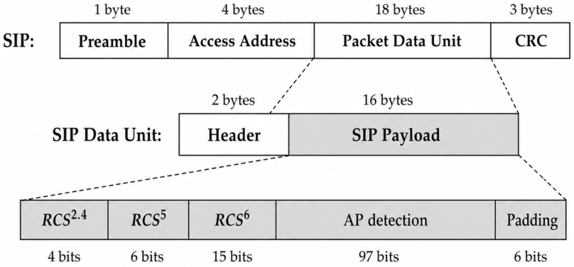
We next summarize the SIP fields used to exchange scan information. An SIP carries information on scan responsibilities and AP detections through BLE advertising. Figure 1 shows the SIP field layout for the tri-band channel-set model. The RCS field records the channel sets that the sender scans directly, and the AP detection field records individual Wi-Fi channels where APs were observed. The channel-set definitions and the bitmap interpretation are given in Section 3.2.

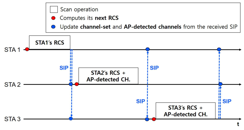
Figure 2 illustrates the SIP exchange process among three STAs. Each STA receives SIPs from BLE neighbors, accumulates the RCS fields to identify channel sets already covered by neighbor scan responsibilities, and incorporates the AP detection information reported in those SIPs into its local view. Operationally, an STA checks the Wi-Fi channels in its own RCS channel sets and may also check individual channels reported as APs detected in received neighbor SIPs. The former defines direct scan responsibility, while the latter prevents the STA from ignoring channels where neighbors have already observed APs. After updating this local view, the STA computes its next RCS. The mathematical analysis in Section 4 abstracts the RCS part of this operation into a graph-covering problem.

3.2. Tri-Band Channel-Set Space and Bitmap Fields

Let

$$\mathcal{B}=\{2.4,5,6\}$$

(1)

be the set of Wi-Fi bands considered in the model. For each band $m\in \mathcal{B}$, let

$${\mathcal{C}}_m=\{C_m^1,C_m^2,\dots ,C_m^{k_m}\}$$

(2)

denote the collection of channel sets in that band, where $k_m=\left|{\mathcal{C}}_m\right|$. The complete channel-set space is

$$\mathcal{C}=\bigcup _{m\in \mathcal{B}}{\mathcal{C}}_m,k=\sum _{m\in \mathcal{B}}{k}_m.$$

(3)

The parameterization used in this paper is

$$k_{2.4}=4,k_5=6,k_6=15,k=25.$$

(4)

Thus, the complete channel-set space contains 25 scan-responsibility units.

The 2.4 GHz and 5 GHz channel sets follow the grouping used in the preliminary SplitScan implementation. We use the PSC locations defined for 6 GHz discovery in IEEE 802.11be [5] as anchors for the 6 GHz RCS groups. For each anchor, the nominal 20 MHz channel indices in the corresponding 80 MHz interval form one RCS unit. This grouping provides one compact unit for assigning scan responsibility, while the AP detection bitmap retains the individual channel indices. For the 6 GHz band, let the nominal 20 MHz channel index set be

$${\mathcal{S}}_6=\{1,5,9,\dots ,233\}.$$

(5)

We use the PSC anchors

$$p_j=5+16(j-1),j=1,2,\dots ,15,$$

(6)

and define the 6 GHz channel sets as

$$C_6^j=\{p_j-4,p_j,p_j+4,p_j+8\}\cap {\mathcal{S}}_6,j=1,2,\dots ,15.$$

(7)

The construction yields 15 RCS units. The first 14 units contain four channel indices, while the final unit is $C_6^{15}=\{225,229,233\}$ because ${\mathcal{S}}_6$ ends at 233. The 6 GHz band therefore contributes $k_6=15$ bits to the tri-band RCS field.

The three bands differ only in how their physical channels are grouped into channel sets. Once the groups in

Table 3. Band-indexed channel-set definitions used in the SplitScan model.

Band	RCS Unit	Included Wi-Fi Channel Indices
2.4 GHz	$C_{2.4}^1$	$\{1,2,3\}$
	$C_{2.4}^2$	$\{4,5,6\}$
	$C_{2.4}^3$	$\{7,8,9,10\}$
	$C_{2.4}^4$	$\{11,12,13,14\}$
5 GHz	$C_5^1$	$\{36,40,44,48\}$
	$C_5^2$	$\{52,56,60,64\}$
	$C_5^3$	$\{100,104,108,112\}$
	$C_5^4$	$\{116,120,124,128\}$
	$C_5^5$	$\{132,136,140,149\}$
	$C_5^6$	$\{153,157,161,165\}$
6 GHz	${\displaystyle C_6^j}$ ${\displaystyle j=1,\dots ,15}$	${\displaystyle \begin{array}{cc}\hfill C_6^j& =\{p_j-4,p_j,p_j+4,p_j+8\}\cap {\mathcal{S}}_6,\hfill \\ \hfill \mathrm{where}{p}_j& =5+16(j-1),{\mathcal{S}}_6=\{1,5,9,\dots ,233\}.\hfill \end{array}}$

Note: Wi-Fi channel availability varies with the regulatory domain and device configuration. The 6 GHz row uses the United States FCC 5.925–7.125 GHz allocation. The 2.4 and 5 GHz rows reproduce the legacy channel list used in the preliminary implementation [2]. Channel 144 was not included in that reported configuration. The fifth 5 GHz RCS group in that configuration was $\{132,136,140,149\}$. These rows define the scan-responsibility units used in the analysis.

are defined, every $C_m^{\ell }$, regardless of m, is treated as one RCS unit by the RCS rule and by the graph formulation.

An SIP contains two bitmap fields: an RCS field and an AP detection field. The channel sets in $\mathcal{C}$ are placed in a fixed order, for example,

$$C_{2.4}^1,\dots ,C_{2.4}^{k_{2.4}},C_5^1,\dots ,C_5^{k_5},C_6^1,\dots ,C_6^{k_6}.$$

The RCS field follows this order. The bit associated with $c\in \mathcal{C}$ is one when the sender itself scans the Wi-Fi channels in c. This is called directly scanning c, in contrast to learning about c through a received SIP. The AP detection field is a bitmap over individual Wi-Fi channels. A bit is one if the sender observed at least one AP on that channel during its scan. The padding bits shown in Figure 1 carry no scan information and are included only for byte alignment. The RCS field specifies which channel sets are scanned by the sender, and its bits become the binary assignment variables in Section 4. The AP detection field remains operational information for later local scanning decisions.

3.3. Local RCS Selection Rule

The RCS rule is the local decision rule by which STA i selects the channel sets that it will directly scan. For each band $m\in \mathcal{B}$, the rule operates on the band-specific bitmap ${\mathrm{RCS}}_i^m$ over ${\mathcal{C}}_m$. The resulting band-specific bitmaps are then combined to form the full RCS bitmap ${\mathrm{RCS}}_i$.

At the beginning of a scanning period, $N_i$ is empty and ${\mathrm{nRCS}}_i$ is initialized to the all-zero bitmap over $\mathcal{C}$. When STA i receives an SIP from neighbor j, it updates its neighbor list and the accumulated neighbor RCS bitmap as follows:

$$N_i\leftarrow N_i\cup \left\{j\right\},{\mathrm{nRCS}}_i\leftarrow {\mathrm{nRCS}}_i\vee {\mathrm{RCS}}_j.$$

(8)

Here, $N_i$ is the set of BLE neighbors from which STA i has received SIPs. The operation ∨ is bit-wise OR. Therefore, ${\mathrm{nRCS}}_i$ marks every channel set that at least one received neighbor reports as its scan responsibility. In SplitScan terms, ${\mathrm{nRCS}}_i$ is STA i’s accumulated view of neighbor-reported scan responsibilities.

For STA i and band m, the candidate set of possible band-m RCS bitmaps is

$${\mathcal{Q}}_i^m=\left\{b\in {\{0,1\}}^{k_m}:{\left[b\right]}_{\ell }=1\mathrm{for}\mathrm{all}\ell \mathrm{such}\mathrm{that}{\left[{\mathrm{nRCS}}_i^m\right]}_{\ell }=0\right\}.$$

(9)

The set ${\mathcal{Q}}_i^m$ contains exactly the band-m bitmaps that include all channel sets not covered by the accumulated neighbor RCS information. Thus, any zero bit in ${\mathrm{nRCS}}_i^m$ must be selected by STA i in its own RCS.

STA i also computes a local load-sharing threshold

$${\theta }_i^m=⌈{\displaystyle \frac{k_m}{|N_i|+1}}⌉,$$

(10)

where $\lceil ·\rceil$ denotes the ceiling. The denominator $|N_i|+1$ is the number of STAs that can contribute to STA i’s local view, namely, the received BLE neighbors plus STA i itself. Thus, ${\theta }_i^m$ is the minimum integer number of band-m channel sets that STA i should carry if the band were evenly shared within its local BLE neighborhood.

STA i’s selected band-m RCS is then

$${\mathrm{RCS}}_i^m\in \underset{b\in {\mathcal{Q}}_i^m,n\left(b\right)\ge {\theta }_i^m}{\arg \min }n\left(b\right),$$

(11)

where $n\left(b\right)$ is the Hamming weight of bitmap b. Equation (11) says that STA i first satisfies the missing-coverage requirement in (9), then satisfies the local load-sharing threshold in (10), and finally chooses the smallest bitmap that satisfies both requirements. In operational terms, STA i scans every channel set that its received neighbors fail to cover and adds only as many extra channel sets as needed to avoid becoming a pure free rider.

This locality is important. STA i uses only SIPs received during the current scanning period and does not require global BLE topology information. The next section formulates this local operation as a graph problem and analyzes its coverage and load implications.

4. Graph-Theoretic Formulation and Analysis

We now characterize cooperative scanning as a graph-covering problem. Unlike the protocol description, which is expressed in terms of SIP fields and RCS bitmaps, this section abstracts each STA as a graph node, and each channel set as an item that must be covered in every closed BLE neighborhood. The resulting formulation exposes the coverage requirement, the load-balancing objective, and the topology-driven limits of cooperative scanning.

The protocol variable $N_i$ records the neighbors from which STA i has received SIPs during a scanning period. In the graph model, we use the calligraphic notation ${\mathcal{N}}_i$ for the BLE neighbors reachable from STA i in the underlying graph.

This section first defines the BLE graph and closed neighborhoods, and then uses them to state feasibility, an ideal min–max reference problem, topology-driven limits, and the local load behavior of the distributed RCS rule.

4.1. BLE Neighborhood Graph Model

In SplitScan, an STA can use scan information only from itself and from STAs whose SIPs it can receive over BLE. We model this one-hop BLE information exchange relation as an undirected graph

$$G=(\mathcal{V},\mathcal{E}),$$

(12)

where each vertex is an STA and each edge indicates that two STAs can exchange SIPs over BLE. In the deterministic analysis, the BLE graph is treated as static during one scanning period, and SIP delivery over an edge is assumed to be reliable. Packet loss and redundant reporting are introduced separately in the robustness analysis.

For STA i, the open BLE neighborhood is

$${\mathcal{N}}_i=\{j\in \mathcal{V}:(i,j)\in \mathcal{E}\}.$$

(13)

This set contains the other STAs whose SIPs can be received by STA i.

The closed BLE neighborhood is

$${\mathcal{N}}_i^{+}={\mathcal{N}}_i\cup \left\{i\right\}.$$

(14)

The closed neighborhood represents the STAs whose scan information is available to STA i: its own direct scan, and the SIP reports received from BLE neighbors. Therefore, a channel set is locally available to STA i if at least one STA in ${\mathcal{N}}_i^{+}$ directly scans it.

4.2. RCS Assignment Variables and Feasibility

We next express RCS bitmaps as binary assignment variables. For each STA i and channel set c, define

$$x_{i,c}=\left\{\begin{array}{cc}1,\hfill & \mathrm{if}\mathrm{STA}i\mathrm{directly}\mathrm{scans}\mathrm{channel}\mathrm{set}c,\hfill \\ 0,\hfill & \mathrm{otherwise}.\hfill \end{array}\right.$$

(15)

Thus, $x_{i,c}$ is the graph-theoretic version of one RCS bit. If $x_{i,c}=1$, channel set c is part of STA i’s scan responsibility. If $x_{i,c}=0$, STA i does not scan c directly and must rely on another STA in its closed neighborhood for that information.

The key mathematical observation is that STA i does not need to directly scan every channel set by itself. For STA i to have local information about channel set c, at least one STA in ${\mathcal{N}}_i^{+}$ must directly scan c. This gives the closed-neighborhood coverage constraint

$$\sum _{j\in {\mathcal{N}}_i^{+}}{x}_{j,c}\ge 1,\forall i\in \mathcal{V},c\in \mathcal{C}.$$

(16)

For a fixed STA i and channel set c, the left-hand side counts how many STAs in ${\mathcal{N}}_i^{+}$ directly scan c. The constraint requires at least one such STA. In SplitScan terms, STA i either scans c using its own Wi-Fi interface or obtains scan information for c from a BLE neighbor that scanned c and reported it through an SIP.

Definition 1

(Feasible cooperative scanning assignment). An assignment $x=\left\{x_{i,c}\right\}$ is feasible if it satisfies (16). Equivalently, for every STA i and every channel set c, at least one STA in ${\mathcal{N}}_i^{+}$ directly scans c.

The assignment $x_{i,c}=1$ for all $i\in \mathcal{V}$ and $c\in \mathcal{C}$, in which every STA directly scans every channel set, satisfies (16). SplitScan seeks a sparser feasible assignment by allowing neighboring STAs to share scan responsibility through SIPs.

For a fixed channel set c, let

$$S_c=\{i\in \mathcal{V}:x_{i,c}=1\}.$$

(17)

The set $S_c$ is the set of STAs that directly scan channel set c. Condition (16) is equivalent to requiring ${\mathcal{N}}_i^{+}\cap S_c\ne \varnothing$ for every STA i. In graph-theoretic terms, $S_c$ is a dominating set of G [19]. Therefore, cooperative scanning can be viewed as choosing one dominating set for each channel set while controlling how many of these scanner sets include each STA.

4.3. Centralized Min–Max Load Reference

The RCS rule used by SplitScan is distributed. Each STA chooses its RCS using only the RCS fields received from its BLE neighbors. To evaluate the cost of this local decision-making, we compare it with an ideal reference problem in which a central controller knows the entire BLE graph and assigns all RCS bitmaps at once.

The first question is what objective should represent the ideal assignment. For STA i, define its RCS load as

$$L_i=\sum _{c\in \mathcal{C}}{x}_{i,c}.$$

(18)

This is the number of channel sets that STA i scans directly.

A total-load objective can concentrate many channel sets on a small number of well-positioned STAs. This is undesirable because the largest RCS load determines the worst scan delay and energy burden. We therefore use a min–max objective that minimizes the maximum number of channel sets assigned to any STA:

$$\begin{array}{cc}\hfill \underset{x,z}{min}& z\hfill \end{array}$$

(19)

$$\begin{array}{cccc}\hfill \mathrm{s}.\mathrm{t}.& \sum _{j\in {\mathcal{N}}_i^{+}}{x}_{j,c}\ge 1,\hfill & \hfill & \forall i\in \mathcal{V},c\in \mathcal{C},\hfill \end{array}$$

(20)

$$\begin{array}{cccc}\hfill & \sum _{c\in \mathcal{C}}{x}_{i,c}\le z,\hfill & \hfill & \forall i\in \mathcal{V},\hfill \end{array}$$

(21)

$$\begin{array}{cccc}\hfill & x_{i,c}\in \{0,1\},\hfill & \hfill & \forall i\in \mathcal{V},c\in \mathcal{C}.\hfill \end{array}$$

(22)

This optimization problem is an ILP. Constraint (20) is the feasibility condition from Definition 1. Constraint (21) makes z an upper bound on every STA’s RCS load. Minimizing z therefore minimizes the largest direct scanning burden among all STAs.

The AP detection field reports where APs were observed and can guide later local scan decisions. The closed-neighborhood coverage constraint is instead determined by the RCS assignment, namely, which STA directly scans each channel set. Thus, the deterministic reference problem is expressed in terms of $x_{i,c}$.

Let $z^{★}$ denote the optimal value of (19)–(22). We use $z^{★}$ as an analytical reference value. It represents the best max-load balance achievable when the entire BLE graph is known and all RCS bitmaps are assigned jointly.

Proposition 1

(NP-hardness of the reference feasibility problem). Given G, k, and a load limit z, deciding whether there exists a feasible assignment with RCS load at most z for every STA is NP-hard when k is part of the input.

Proof. 

We reduce from the domatic-number decision problem, which is NP-complete [20]. Given an instance $(G,k)$ of that problem, construct the reference feasibility problem on the same graph G with k channel sets and load limit $z=1$. If G has a domatic partition with at least k dominating sets, merge any extra sets if necessary to obtain k disjoint dominating sets $D_1,\dots ,D_k$. Assign channel set c to exactly the STAs in $D_c$. Then, each channel set is covered in every closed neighborhood, and each STA is assigned to at most one channel set, so the load limit $z=1$ is satisfied.

Conversely, suppose that there is a feasible assignment with $z=1$. For each channel set c, let $S_c=\{i\in \mathcal{V}:x_{i,c}=1\}$. The coverage constraint implies that every $S_c$ dominates G, and the load limit $z=1$ implies that the sets $S_1,\dots ,S_k$ are pairwise disjoint. Any unassigned vertices can be added to one of these sets without destroying domination, so G has a domatic partition with at least k dominating sets. Thus, the constructed instance is feasible if and only if the original domatic-number instance is feasible. Since the reduction is polynomial and the domatic-number decision problem is NP-complete, the reference feasibility problem is NP-hard. □

Consequently, $z^{★}$ serves as the centralized reference for the minimum achievable maximum RCS load under the closed-neighborhood coverage constraint. Comparing SplitScan with $z^{★}$ measures the additional load associated with decisions based on received neighbor SIPs.

4.4. Topology-Dependent Limits of Cooperative Scanning

The centralized min–max reference problem describes the best possible maximum RCS load when the entire BLE graph is known. However, this best possible load is still constrained by the BLE topology. The following results identify two limits determined by the BLE graph. The first gives a lower bound determined by each STA’s closed-neighborhood size. The second evaluates the fully connected BLE topology $G=K_n$, where every STA can receive every other STA’s SIP, and shows that the best possible maximum RCS load is $\lceil k/n\rceil$.

Theorem 1

(Local lower bound). For any BLE graph G, the optimal value of (19)–(22) satisfies

$$z^{★}\ge \underset{i\in \mathcal{V}}{\max }⌈{\displaystyle \frac{k}{|{\mathcal{N}}_i|+1}}⌉.$$

(23)

Proof. 

Consider an arbitrary STA i, and let z be any feasible upper bound on the RCS load. If every STA has an RCS load of at most z, then the STAs in ${\mathcal{N}}_i^{+}$ can collectively provide at most $z|{\mathcal{N}}_i^{+}|$ channel-set assignments visible to STA i. Feasibility requires all k channel sets to appear at least once within this closed neighborhood. Thus, $z|{\mathcal{N}}_i^{+}|\ge k$. Since $|{\mathcal{N}}_i^{+}|=|{\mathcal{N}}_i|+1$ and z is an integer, $z\ge \lceil k/\left(\right|{\mathcal{N}}_i|+1)\rceil$. This holds for every STA i and every feasible z; therefore, it also holds for the optimal value $z^{★}$. Taking the maximum over i proves the claim. □

Theorem 1 gives a topology-dependent lower bound on the maximum RCS load that no feasible assignment can avoid. It therefore provides a reference for assessing the additional load associated with a particular RCS selection rule. If an STA has no BLE neighbor, then $|{\mathcal{N}}_i|=0$, and the bound gives $z^{★}\ge k$. Thus, an isolated STA must scan every channel set because no neighbor can provide scan information through SIPs. If an STA has only a few neighbors, then its small closed neighborhood must still cover all k channel sets. This forces at least one STA in that local region to carry a larger RCS load. Low-degree STAs therefore create worst-node bottlenecks.

Theorem 2

(Complete-graph optimum). If the BLE graph is fully connected, $G=K_n$, then

$$z^{★}=⌈{\displaystyle \frac{k}{n}}⌉.$$

(24)

Proof. 

If $G=K_n$, then ${\mathcal{N}}_i^{+}=\mathcal{V}$ for every STA i. Theorem 1 gives $z^{★}\ge \lceil k/n\rceil$. For the reverse inequality, assign the k channel sets to the n STAs in round-robin order. Then, every channel set is scanned by exactly one STA, and because every STA’s closed neighborhood is $\mathcal{V}$, the coverage constraint is satisfied for every STA and every channel set. Each STA scans at most $\lceil k/n\rceil$ channel sets, so this construction gives a feasible assignment with a maximum RCS load of at most $\lceil k/n\rceil$. Hence, $z^{★}\le \lceil k/n\rceil$. Together with the lower bound, this proves that $z^{★}=\lceil k/n\rceil$. □

Theorem 2 gives the centralized optimum under full BLE connectivity. When every STA can receive every other STA’s SIP, each channel set needs only one direct scanner, and the best centralized assignment distributes the k channel sets as evenly as possible across the n STAs. The value $\lceil k/n\rceil$ therefore serves as a dense-connectivity baseline for interpreting the distributed RCS rule and the corresponding simulations. The intuition is that, as BLE neighborhoods grow, one STA’s direct scan can benefit more neighboring STAs through SIP exchange.

Together, Theorems 1 and 2 describe the two extremes of topology-dependent behavior. Sparse or poorly connected regions force high local load, while full BLE connectivity allows the channel-set space to be divided almost evenly. This explains why cooperative scanning can perform very differently under isolated, random geometric, grid, and complete BLE topologies.

4.5. Distributed RCS Selection and Local Load

This subsection derives the local coverage and load properties of the distributed RCS rule used by SplitScan. Using the RCS bitmaps received from its BLE neighbors, each STA chooses a local RCS that covers channel sets not covered by those neighbors while keeping its own load small.

For STA i and band $m\in \mathcal{B}$, define

$$U_i^m=\{\ell \in \{1,\dots ,k_m\}:{\left[{\mathrm{nRCS}}_i^m\right]}_{\ell }=0\}$$

(25)

as the set of band-m channel-set indices not covered by the RCS fields received from STA i’s BLE neighbors. Let $u_i^m=\left|U_i^m\right|$. In SplitScan terms, $U_i^m$ contains the band-m channel sets that STA i’s received neighbors do not report as their scan responsibilities. With the current information from received SIPs, these channel sets must be included in STA i’s own RCS.

Theorem 3

(Local coverage and load of the RCS selection rule). For every STA i and band $m\in \mathcal{B}$, the RCS selected by (11) satisfies

$${\mathrm{RCS}}_i^m\vee {\mathrm{nRCS}}_i^m=11_{k_m}.$$

(26)

Moreover, if ${\theta }_i^m$ is defined by (10), then

$$n\left({\mathrm{RCS}}_i^m\right)=\max \{u_i^m,{\theta }_i^m\}.$$

(27)

Proof. 

By definition of ${\mathcal{Q}}_i^m$ in (9), every candidate bitmap contains all channel-set indices not covered by ${\mathrm{nRCS}}_i^m$. Therefore, the selected RCS sets every bit that is zero in ${\mathrm{nRCS}}_i^m$, proving (26). Any feasible candidate must include the $u_i^m$ channel-set indices not covered by ${\mathrm{nRCS}}_i^m$ and must have a Hamming weight of at least ${\theta }_i^m$. Thus, its Hamming weight is at least $\max \{u_i^m,{\theta }_i^m\}$. Conversely, a candidate bitmap with Hamming weight $\max \{u_i^m,{\theta }_i^m\}$ is obtained by including all channel-set indices in $U_i^m$ and, if necessary, adding already covered indices until the threshold is reached. Since (11) minimizes the Hamming weight over the feasible candidates, (27) follows. □

Equation (26) states the local coverage guarantee of the RCS selection rule. STA i’s own RCS, combined with the accumulated neighbor RCS information, covers every channel set in band m. Equation (27) gives the corresponding local load. STA i’s band-m load is the larger of the number of channel sets not covered by the received neighbor RCS information and the local load-sharing threshold. Thus, two STAs with the same number of received neighbors can still have different loads if those neighbors report different channel-set patterns.

Theorem 3 describes what happens each time an STA selects its RCS from the SIPs currently available to it. The complete distributed operation consists of many such decisions made by different STAs over time. Their combined effect can depend on the order and timing of those decisions and on how an STA chooses among multiple minimum-load RCS candidates.

Remark 1

(Network-wide performance of repeated RCS decisions). Even for a fixed BLE graph, a worst-case comparison with the centralized reference requires the order and timing of STA decisions and the rule for choosing among multiple minimum-load RCS candidates to be specified. Deriving a bound on the ratio between the resulting maximum RCS load and the centralized optimum remains an open problem. Section 6.4 reports empirical comparisons of the maximum RCS load under the asynchronous decision schedule and coverage completion procedure used in the simulations.

5. Stochastic Scaling and Robustness

The deterministic analysis explains how a fixed BLE graph constrains RCS assignment. We now study how the expected RCS load changes with spatial STA density, how this load reduction translates into an energy condition, and how reliability changes when BLE advertisements are lost.

5.1. Random Geometric Scaling Model

Suppose that STA locations are modeled by a homogeneous Poisson point process with density ${\lambda }_s$, and two STAs are BLE neighbors when their distance is at most $R_B$. Under the infinite-plane approximation, the degree D, i.e., the number of BLE neighbors of a representative STA, follows

$$D\sim \mathrm{Poisson}\left(\mu \right),\mu ={\lambda }_s\pi R_B^2.$$

(28)

To obtain a tractable analytical reference, assume that the k channel sets can be shared fractionally and evenly among the STAs in a representative closed neighborhood. If $D=d$, this closed neighborhood contains $d+1$ STAs, including the representative STA itself. The corresponding ideal per-STA RCS load is then $k/(d+1)$. Averaging over the random degree D gives

$$\mathbb{E}\left[L_{\mathrm{ideal}}\right]\approx \mathbb{E}\left[{\displaystyle \frac{k}{D+1}}\right]=k{\displaystyle \frac{1-e^{-\mu }}{\mu }}.$$

(29)

The last equality follows from the Poisson distribution in (28).

The quantity in (29) serves as a fractional reference for the density trend. It isolates how the mean BLE neighborhood size affects the RCS load when the k channel sets are evenly shared over a representative closed neighborhood. The distributed RCS selection rule operates on integer channel sets, handles the channel groups of each band, and compensates for channel sets not covered by received neighbor RCSs.

To compare channel-set spaces with different k, we normalize the load by k. This normalized load represents the fraction of the channel-set space scanned by a representative STA:

$${\displaystyle \frac{\mathbb{E}\left[L_{\mathrm{ideal}}\right]}{k}}\approx {\displaystyle \frac{1-e^{-\mu }}{\mu }}.$$

(30)

Equation (30) shows that the normalized reference depends only on the mean BLE neighborhood size $\mu$. Thus, the absolute load in (29) scales with k, whereas the load fraction is controlled by the BLE neighborhood size.

The isolated-node probability under the same degree model is

$$\mathbb{P}[D=0]=e^{-\mu }.$$

(31)

This quantity matters because isolated STAs cannot use neighbor SIPs. By Theorem 1, an isolated STA has $|{\mathcal{N}}_i|=0$, so the lower bound becomes k. Such an STA must therefore carry all k channel sets in its own RCS because no neighbor can provide scan information.

5.2. Energy Break-Even Condition

Let $E_{\mathrm{conv}}$ be the energy consumed by a full Wi-Fi scan. This scan visits all channels in the considered configuration without using cooperative SIP information. Let $E_{\mathrm{SS}}$ be the energy of one SplitScan cycle:

$$E_{\mathrm{SS}}=E_{\mathrm{WiFi},\mathrm{RCS}}+E_{\mathrm{WiFi},\mathrm{APdet}}+E_{\mathrm{BLE}}.$$

(32)

Here, $E_{\mathrm{WiFi},\mathrm{RCS}}$ is the energy spent scanning assigned RCS channel sets, $E_{\mathrm{WiFi},\mathrm{APdet}}$ is the energy spent checking channels reported as AP-detected in received SIPs when such checking is needed, and $E_{\mathrm{BLE}}$ is the BLE advertising and listening overhead. SplitScan has an energy advantage when

$$E_{\mathrm{BLE}}+E_{\mathrm{WiFi},\mathrm{APdet}}<E_{\mathrm{conv}}-E_{\mathrm{WiFi},\mathrm{RCS}}.$$

(33)

Using the fractional load reference in (29), approximate Wi-Fi scan energy as proportional to direct RCS load. This gives

$$E_{\mathrm{WiFi},\mathrm{RCS}}\approx E_{\mathrm{conv}}{\displaystyle \frac{\mathbb{E}\left[L_{\mathrm{ideal}}\right]}{k}}.$$

Substituting (30) into (33) gives the approximate break-even condition:

$$E_{\mathrm{BLE}}+E_{\mathrm{WiFi},\mathrm{APdet}}<E_{\mathrm{conv}}\left(1-{\displaystyle \frac{1-e^{-\mu }}{\mu }}\right).$$

(34)

This condition states that the BLE and AP detection overhead must be smaller than the Wi-Fi scan energy saved by reducing direct RCS scanning.

5.3. Robust SplitScan-r Under BLE Packet Loss

The deterministic coverage condition in (16) treats a channel set scanned inside ${\mathcal{N}}_i^{+}$ as available to STA i. This corresponds to reliable SIP delivery over BLE edges during the scanning period. When BLE advertisements are lost, however, a feasible RCS assignment may fail to provide scan information to a receiver. Robust SplitScan-r addresses this loss by requiring each channel set to be directly scanned by at least r STAs in the closed neighborhood.

The redundant coverage condition is

$$\sum _{j\in {\mathcal{N}}_i^{+}}{x}_{j,c}\ge r,\forall i\in \mathcal{V},c\in \mathcal{C}.$$

(35)

For a fixed STA i and channel set c, the left-hand side counts how many STAs in ${\mathcal{N}}_i^{+}$ directly scan c. The threshold r requires this count to be r or larger, so the channel set is represented multiple times within STA i’s closed neighborhood. The baseline coverage condition in (16) corresponds to $r=1$.

Assume that each BLE report that could provide scan information for c is delivered with probability q, independently across reports. For a fixed STA i and a fixed channel set c, let $P_{\mathrm{miss}}(i,c)$ denote the probability that STA i obtains no usable scan information for c. If all r reports are lost, then STA i misses the information for c. Thus,

$$P_{\mathrm{miss}}(i,c)\le {(1-q)}^r.$$

(36)

This bound is conservative because STA i’s own scan does not require BLE delivery, and the closed neighborhood may contain more than r reports for c.

Suppose that the design goal is that, for any particular STA and any particular channel set, the probability of receiving no usable scan information should be at most $ϵ$. In the notation above, this means that $P_{\mathrm{miss}}(i,c)\le ϵ$. It is sufficient to choose r so that ${(1-q)}^r\le ϵ$. For $0<q<1$ and $0<ϵ<1$, this gives

$$r\ge ⌈{\displaystyle \frac{\log ϵ}{\log (1-q)}}⌉.$$

(37)

This follows by taking logarithms of ${(1-q)}^r\le ϵ$ and noting that $\log (1-q)<0$.

The redundancy level r creates a tradeoff between reliability and scanning load. A larger r lowers the miss probability in (36), but it also assigns more STAs to each channel set and, therefore, increases the scanning energy. BLE neighbor-discovery reliability studies provide the practical background for this tradeoff [16,17].

The bound in (36) applies to one fixed STA and one fixed channel set. An STA, however, needs scan information for all k channel sets. For a fixed STA i, let $A_c^{\left(i\right)}$ be the event that STA i misses scan information for channel set c. The probability that STA i misses at least one channel set is

$$P_{\mathrm{any}\mathrm{miss}}\left(i\right)=\mathrm{Pr}\left[\bigcup _{c\in \mathcal{C}}{A}_c^{\left(i\right)}\right].$$

By the union bound,

$$P_{\mathrm{any}\mathrm{miss}}\left(i\right)\le \sum _{c\in \mathcal{C}}\mathrm{Pr}\left[A_c^{\left(i\right)}\right]\le k{(1-q)}^r.$$

(38)

Thus, a larger channel-set space requires either a larger redundancy level or a higher BLE delivery probability to keep the probability of missing any channel-set information small for a given STA.

6. Numerical Validation

This section validates the preceding analysis through Monte Carlo simulations. The simulations first examine how BLE neighborhood density and graph topology affect scanning load, scan time, and energy. We then compare RCS assignment approaches that use different amounts of network information and coordination, and we evaluate how redundancy affects reliability and energy under BLE packet loss.

6.1. Simulation Setup

Unless otherwise noted, STAs are placed uniformly in a disk, and BLE edges are created using a distance threshold. In experiments that include APs, APs are placed independently and each AP is assigned an operating channel sampled uniformly from the simulated channel space. We used 300 Monte Carlo trials for the density and topology experiments, 100 trials for the RCS assignment comparison in Section 6.4, and 200 trials for the packet loss experiment. The density, topology, RCS assignment, and packet loss experiments used the tri-band channel-set model defined in Section 3.2.

The time and energy ratios use the two-band scan time and energy baseline from the preliminary SplitScan measurements. The density experiment also reports absolute and normalized RCS load to separate the effect of channel-set cardinality from the effect of BLE neighborhood size.

6.2. Density Scaling and Channel-Set Cardinality

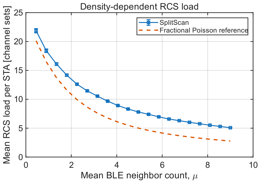
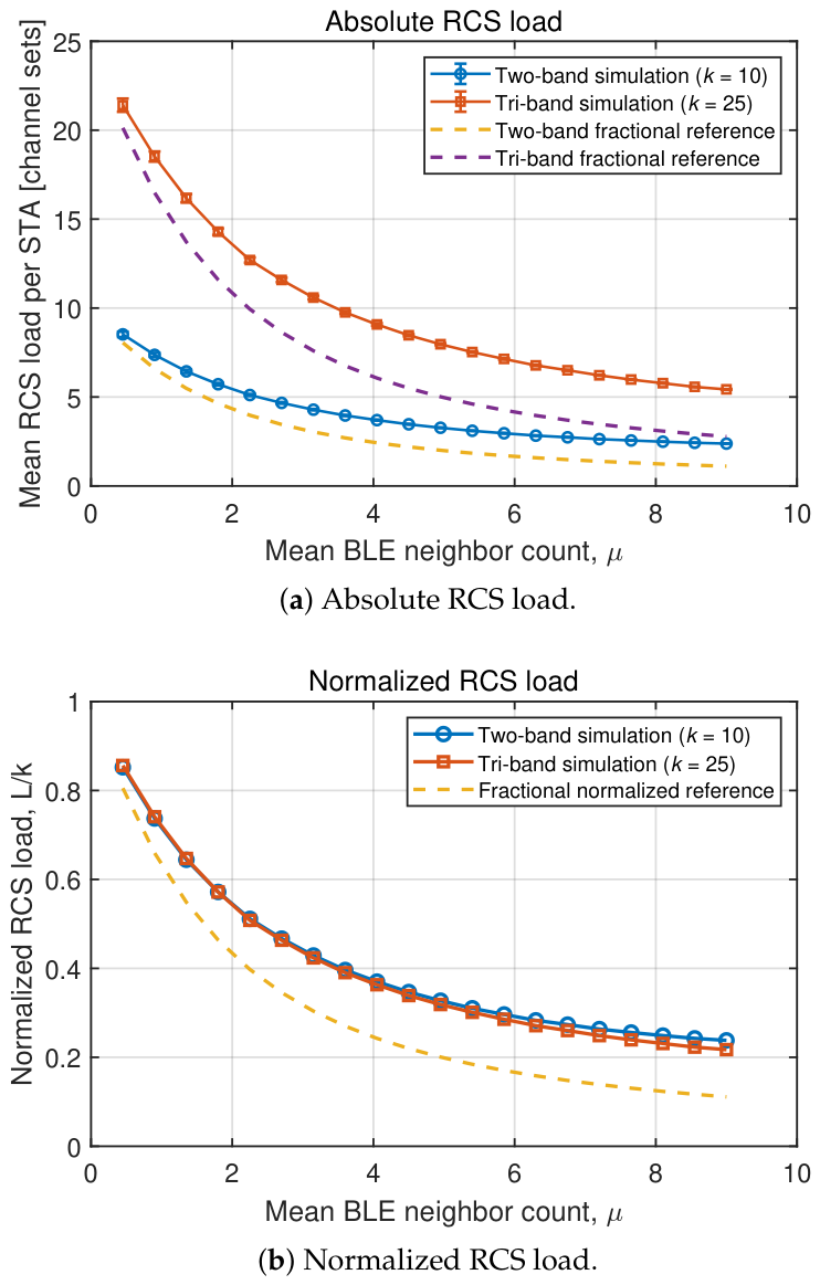
Figure 3 shows that the empirical RCS load decreases as the mean BLE neighborhood size increases. The dashed curve is a fractional Poisson reference derived from (29). It assumes that the k channel sets can be divided evenly and fractionally among the $D+1$ STAs in a representative closed neighborhood. The simulated RCS load stays above this reference because SplitScan selects integer bitmap entries, applies the selection rule separately by band, and must include channel sets not covered by received neighbor RCS information. The remaining gap reflects boundary effects in the finite disk and heterogeneous closed neighborhoods that are not captured by the fractional Poisson reference.

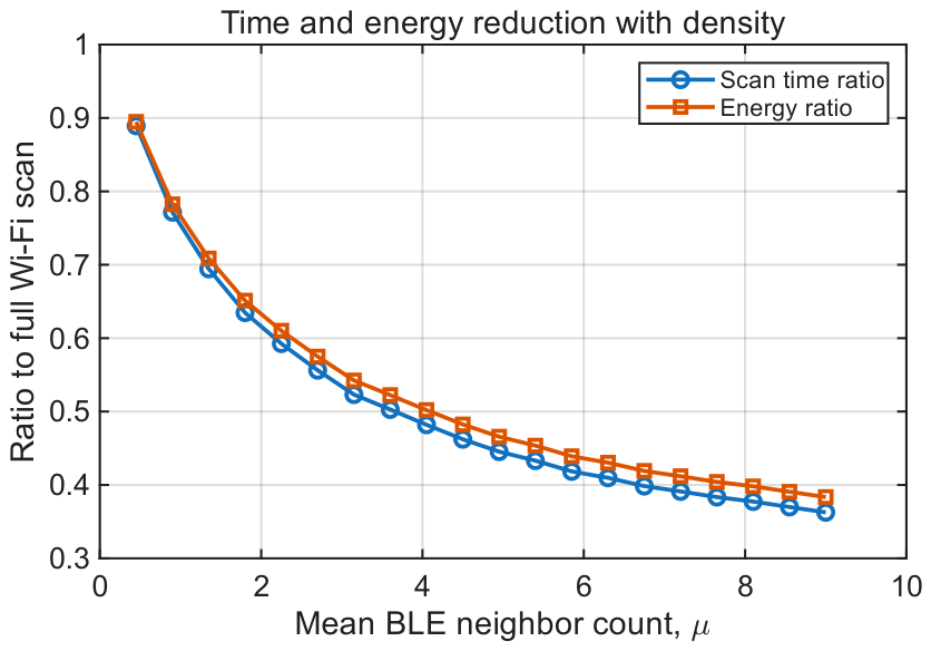
Figure 4 uses the two-band scan time and energy baseline from the preliminary measurements to translate RCS load reduction into operational scan cost. For each density point, the scan time ratio is the simulated mean SplitScan scan time divided by the time of a full Wi-Fi scan in this two-band baseline. The energy ratio is computed in the same way, using the simulated mean SplitScan energy and the energy of the same full Wi-Fi scan. Thus, a ratio below one means that SplitScan uses less scan time or energy than a full Wi-Fi scan. Both ratios decrease as the mean BLE neighborhood size increases, because denser neighborhoods allow STAs to reuse more neighbor scan information and directly scan fewer channel sets. The isolated-node fraction also decreases qualitatively with the Poisson trend $e^{-\mu }$, which helps explain why sparse deployments provide weaker cooperative gain.

The same density sweep was used to examine the effect of channel-set cardinality. Figure 5 compares the two-band 2.4/5 GHz configuration with $k=10$ and the tri-band 2.4/5/6 GHz configuration with $k=25$. Figure 5a shows that the tri-band configuration has a larger absolute RCS load, consistent with its larger channel-set cardinality and the corresponding fractional reference. Figure 5b shows that, after normalizing by k, the two simulated curves follow similar density-dependent behavior, consistent with (30).

6.3. Impact of BLE Topology

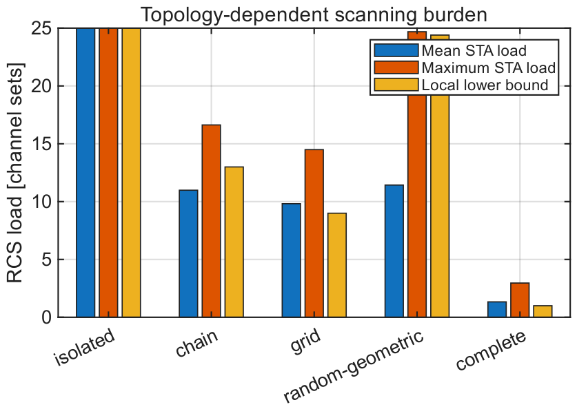
The topology experiment compared isolated, chain, grid, random geometric, and complete BLE graphs using the tri-band channel-set model. In this experiment, $n=30$ STAs were used. For range-based geometric constructions, the BLE range was $R_B=30\mathrm{m}$. The chain topology denotes the path graph $P_n$, in which STAs are connected in a one-dimensional line and the two endpoint STAs have degree one. The grid topology was generated from the first n vertices of an $m\times m$ square lattice, where $m=\lceil \sqrt{n}\rceil$, with lattice spacing $0.85R_B$; BLE edges were then formed by the range threshold $R_B$.

The isolated and complete graphs provide two endpoint cases for interpreting the figure. In an isolated graph, each STA’s closed neighborhood contains only itself, so no STA can reuse scan information from a BLE neighbor. Each STA must therefore carry all k channel sets in its own RCS. In a complete graph, every STA can receive every other STA’s SIP, so a channel set scanned by one STA can be reused by all STAs. This creates the lowest load case under dense BLE connectivity, consistent with the intuition behind Theorem 2.

Figure 6 shows that intermediate topologies depend strongly on closed-neighborhood structure. Chain, grid, and random geometric graphs allow only local reuse, and the random geometric case exhibits a high maximum STA load because low-degree STAs remain bottlenecks. The local lower-bound bars show how much of the worst-node load is imposed by the closed-neighborhood sizes themselves.

6.4. Comparison of RCS Assignment Methods and References

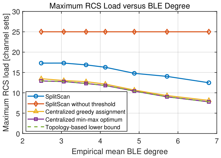
The comparison used $n=16$ STAs, and BLE density was varied by changing the disk radius. The horizontal axis reports the average number of BLE neighbors measured in the retained graphs. Only graphs in which every STA has at least one BLE neighbor are retained. If an isolated STA were included, its closed neighborhood would contain only itself, forcing it to scan all $k=25$ channel sets and fixing the maximum RCS load at 25. Excluding such graphs allows the comparison to focus on how the methods distribute scanning work when cooperation is possible.

For each retained BLE graph, the four assignment methods use the same graph and the same tri-band channel-set space. After the coverage completion procedure described below, their assignments are evaluated using the closed-neighborhood coverage requirement in (16) and the maximum RCS load. The analytical lower bound is computed from the same graph. For clarity, each parenthetical label has the form (how the result is obtained, information used).

• SplitScan (distributed, received neighbor SIPs): At each scheduled scan time, an STA uses the SIPs received from its direct BLE neighbors since its previous scan. It selects every channel set not covered by the accumulated neighbor RCS bitmap and then adds the smallest number of extra channel sets needed to satisfy the load threshold in (10). If several RCS candidates have the same minimum size, the simulation selects one of them at random. An STA does not know the complete BLE graph or the loads of STAs beyond the information contained in its received SIPs.
• SplitScan without the Load Threshold (distributed, received neighbor SIPs): This comparison variant follows the same distributed SIP exchange model as SplitScan but removes the threshold in (10). At each scan, an STA selects only the channel sets not covered by the received neighbor RCS information and does not add channel sets merely to maintain a minimal share of the scanning work. This variant measures the contribution of the load threshold to preventing responsibility from remaining concentrated at one STA.
• Greedy Assignment with Global Information (centralized, complete BLE graph and assignments made so far): A central controller constructs the assignment one channel set at a time. At each step, it knows the complete BLE graph, which closed neighborhoods have already been covered for the current channel set, and the number of channel sets assigned so far to every STA. It selects the STA that maximizes the number of newly covered closed neighborhoods divided by its assigned load plus one. This sequential procedure is a heuristic and does not solve the joint min–max optimization problem.
• Min–Max Optimum (centralized, complete BLE graph): The ILP in (19)–(22) determines all RCS assignments jointly. It minimizes the largest number of channel sets assigned to any STA and returns the exact optimum $z^{★}$.
• Topology-Based Lower Bound (analytical, closed-neighborhood sizes): Unlike the four assignment methods above, this curve is obtained directly from the BLE graph rather than from a constructed RCS assignment. Equation (23) uses the closed-neighborhood sizes to give a topology-imposed lower bound on the maximum RCS load, which provides a common reference for evaluating the four assignment methods.

The two centralized approaches use the same complete BLE graph but differ in how they construct the assignment. The greedy method assigns channel sets sequentially and bases each choice on the coverage and STA loads accumulated so far. The ILP instead determines all RCS assignments jointly and returns the exact minimum possible maximum load. Because the greedy method does not jointly reconsider all assignments, its result is not necessarily optimal.

The two distributed methods update each STA’s RCS at different scheduled scan times. When an STA makes a decision, it may rely on a neighbor’s current SIP and omit a channel set from its own RCS. That neighbor can later change its RCS before the simulation ends. Consequently, the final RCS values collected from all STAs can leave a closed neighborhood without a scanner for a channel set, even though each STA satisfied the selection rule when it made its own decision. To compare these distributed results with the static centralized assignments, we apply the same coverage completion procedure to both distributed methods. If a channel set is not covered by any RCS in a closed neighborhood, it is added to the STA with the smallest current RCS load in that neighborhood. This procedure only adds scanning responsibilities, so it cannot reduce the reported maximum load. The greedy and ILP methods already construct assignments that satisfy the coverage requirement.

After coverage completion, let $x_{i,c}^{\mathrm{SS}}=1$ when channel set c is assigned to STA i in the SplitScan result. The reported value is

$$z_{\mathrm{SS}}=\underset{i\in \mathcal{V}}{\max }\sum _{c\in \mathcal{C}}{x}_{i,c}^{\mathrm{SS}}.$$

The corresponding maximum load is computed in the same way for the variant without the load threshold and for the greedy assignment. The ILP returns $z^{★}$.

Comparing SplitScan with the variant without the load threshold isolates the contribution of (10). Without the load threshold, the missing-coverage rule treats all 25 channel sets identically. Starting from the all-zero RCS state used in the simulation, an STA that has not yet received useful SIP information can therefore select all 25 channel sets, while later STAs that receive its SIP can select few or no channel sets during the distributed update process. Because Figure 7 reports the largest RCS load across STAs rather than the average load, the presence of even one STA carrying all 25 channel sets keeps the maximum load at 25. With the load threshold, each STA retains at least ${\theta }_i^m$ channel sets in band m, even when its neighbors already report broad coverage. These responsibilities are advertised in subsequent SIPs, so an STA that previously carried many channel sets can recognize newly reported neighbor coverage and reduce its own RCS at a later scan decision. Scanning responsibility is consequently spread across more STAs, and the mean maximum load of SplitScan decreases from 17.85 to 13.77 channel sets as BLE connectivity grows. Relative to the value of 25 without the threshold, this corresponds to a reduction of 7.15–11.23 channel sets over the tested density points. The comparison therefore shows that the load threshold replaces a concentrated responsibility pattern with a more balanced distribution of scanning work through repeated SIP exchange.

The two centralized curves are close because both methods use the complete BLE graph. The greedy method constructs the assignment sequentially using the coverage and STA loads accumulated after each choice, whereas the ILP optimizes all RCS assignments jointly. The greedy result remains only 0.18–0.75 channel sets above the ILP optimum over the tested density points. This small gap reflects the difference between sequential greedy choices and joint exact optimization.

SplitScan remains 4.64–5.94 channel sets above the ILP optimum because each STA uses only the SIPs received from its direct BLE neighbors and the number of neighbors from which those SIPs were received. It cannot observe scanning responsibilities or STA loads beyond the information in those SIPs, and different STAs make their decisions at different scan times, so overlapping responsibilities can remain. The observed gap therefore quantifies the load reduction provided by complete network information and centralized coordination. The centralized methods require collection of the full BLE topology and centralized assignment, whereas SplitScan operates through distributed peer SIP exchange. At the same time, SplitScan substantially reduces the maximum load relative to the variant without the threshold. Figure 7 therefore characterizes the relationship between coordination requirements and maximum RCS load under the simulated graphs and decision procedure.

6.5. Reliability and Energy Under BLE Packet Loss

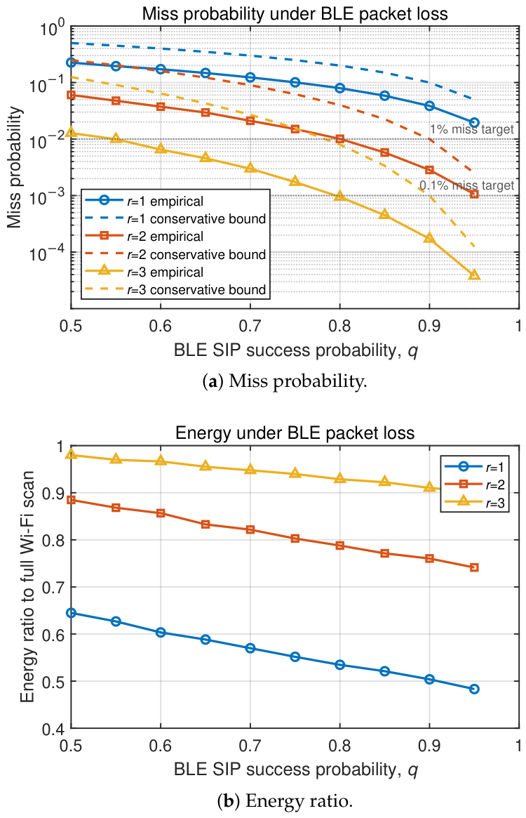
The packet loss experiment evaluated Robust SplitScan-r under BLE packet loss using the tri-band channel-set model. Figure 8a shows the empirical miss probability on a logarithmic scale, together with target miss probabilities of $1\%$ and $0.1\%$ and the conservative bound ${(1-q)}^r$. Figure 8b shows the corresponding energy ratio relative to a full Wi-Fi scan over the same tri-band channel-set space. Increasing r reduces the miss probability but raises the energy ratio because additional STAs scan each channel set.

In the simulated parameter range, $r=2$ balances reliability and energy more effectively than $r=1$, while $r=3$ further reduces miss probability at a higher energy cost.

7. Discussion

The preceding results show that SplitScan depends on two deployment factors: the first is local reuse of scan information through closed BLE neighborhoods, and the second is redundancy against BLE packet loss. This section discusses the deployment implications of these factors and clarifies the scope of the analysis.

7.1. Topology-Dependent Deployment Considerations

SplitScan’s performance is governed by closed-neighborhood structure rather than by STA count alone. The average BLE degree is informative, but local low-degree or isolated STAs determine the worst scanning burden because they have fewer reusable scan reports. The tri-band channel-set model amplifies this effect: dense BLE neighborhoods can distribute the additional 6 GHz channel sets across many STAs, whereas sparse neighborhoods force low-degree STAs to carry more of the enlarged channel-set space.

7.2. Reliability–Energy Tradeoff

Robust SplitScan-r makes reliability tunable through redundant scan responsibility. Increasing r reduces the miss probability approximately as ${(1-q)}^r$, but it increases the scanning load and energy. Larger channel-set spaces make this tradeoff sharper because an STA must maintain reliable information over more channel sets. Hence, a tri-band deployment may require stronger BLE delivery or a larger redundancy level to keep the probability that an STA misses any channel-set information low.

7.3. Practical Implications

Dense BLE Neighborhoods: When most STAs receive SIPs from several different neighbors, scan responsibilities can be distributed across more devices, and the direct RCS burden decreases. The density and topology results indicate that the largest gains are expected in offices, campuses, and similar environments where multiple BLE-capable devices remain within one-hop range during a scanning period.

Sparse or Uneven Neighborhoods: A high average BLE degree can coexist with low-degree boundary STAs. For these STAs, a practical implementation can retain a larger RCS and use a full scan when no usable SIP is received. This fallback preserves channel coverage when only a small number of neighboring reports are available and reflects the fact that the smallest closed neighborhoods determine the maximum scanning burden.

Redundancy Configuration: The redundancy level should reflect the observed reliability of BLE report delivery and the required level of report availability. Increasing r improves the probability that scan information reaches an STA, but it also increases the direct scanning load and Wi-Fi energy consumption. A practical implementation can therefore use a small value of r when BLE delivery is stable and increase r when the measured delivery reliability falls below the required level.

7.4. Limitations

Changing BLE Neighborhoods: The graph model represents the BLE neighborhood as fixed during one scanning period, and the SIPs used by the SIP-based RCS selection procedure are treated as current. In mobile environments, the set of STAs within BLE range can change over time, so an earlier SIP may no longer reflect the STAs that are currently nearby. The local coverage statement therefore applies to the SIP information available when an RCS is selected, while rapid topology changes can invalidate network-wide coverage until updated SIPs are received and new RCS decisions are made. Extending the framework to changing BLE neighborhoods would therefore require recording when each SIP was received and periodically updating the BLE graph.

Correlated Report Losses: The packet loss analysis models BLE report deliveries as independent. Common interference sources or burst losses can instead produce correlated report failures. Under these conditions, the measured delivery reliability may differ from the bound derived under independent delivery. Accordingly, the bound ${(1-q)}^r$ is not a theoretical guarantee when report losses are correlated, and positive correlation can reduce the reliability gain obtained from additional copies. A model that captures such correlation would provide a more detailed basis for selecting the redundancy level in these environments.

Evaluation Scale: The centralized ILP provides an exact reference for the graph sizes evaluated in Section 6.4, while the Monte Carlo study covers the graph sizes and parameter ranges reported in Section 6. The behavior of larger networks and rapidly changing topologies, including convergence across repeated RCS decisions, remains to be evaluated.

Real-World Validation: The preliminary SplitScan study implemented the protocol on Linux laptops with commercial Wi-Fi and Bluetooth interfaces and evaluated both two-STA and eight-laptop dense testbeds [2]. Those experiments demonstrated reductions in scanning time and energy in controlled indoor settings. The present article does not repeat that implementation study, and performance under broader interference conditions, mobility patterns, and heterogeneous hardware remains to be evaluated.

Computation and Communication Overhead: When STA i processes one k-bit RCS field from each of $d_i=\left|{\mathcal{N}}_i\right|$ neighbors during a scanning period, accumulating the received RCS information requires $O\left(d_{i}k\right)$ bit operations. Using the constructive form in Theorem 3, the next RCS can be formed by identifying the channel sets not covered by the received neighbor RCS information and, if needed, adding channel sets until the threshold is reached. This requires $O\left(k\right)$ time and avoids enumerating all candidate bitmaps. The local procedure therefore avoids the centralized ILP and does not require storage of the complete BLE graph. The tri-band SIP contains 25 RCS bits, 97 AP detection bits, and six padding bits, for 128 scan-information bits before BLE framing. In the preliminary implementation, each STA generated one updated SIP after each scan [2]. Thus, n STAs produce $O\left(n\right)$ logical SIP updates per scanning period. The number of physical BLE advertisement packets depends on the advertising interval and timeout. STA i processes $O\left(d_i\right)$ received SIP updates, and the total number of SIP receptions across the network scales as $O\left({\sum }_{i\in \mathcal{V}}{d}_i\right)=O\left(\right|\mathcal{E}\left|\right)$, which becomes $O\left(n^2\right)$ in a fully dense BLE graph. Although the two-STA and eight-laptop experiments operated successfully, BLE contention, convergence time, and signaling overhead in substantially larger dense deployments remain to be quantified.

Security of Exchanged Reports: The present framework assumes that received SIPs are authentic and that their RCS and AP detection fields are truthful. A forged RCS claim can cause neighbors to omit a channel set from direct scanning, while false AP detection information can trigger unnecessary scanning or conceal useful scan information. In a secure extension, corroboration across multiple authenticated reports and a conservative full-scan fallback could limit the effect of an inconsistent report. These mechanisms are not part of the current model, which does not provide an adversarial guarantee. A secure implementation would require source authentication and integrity protection, freshness checks, consistency or corroboration rules across peers, and fallback scanning when reports conflict. Developing and evaluating these mechanisms requires a separate threat model and remains an avenue for future work.

Channel Configuration: The numerical channel-set map represents one regulatory and device configuration. The graph formulation accepts the channel-set collection as an input, so each deployment can construct its RCS bitmap from the channels supported by its regulatory domain and device configuration.

8. Conclusions

This paper presents a graph-theoretic and stochastic analysis of SplitScan for BLE-assisted cooperative Wi-Fi scanning. The main result is that scan-responsibility sharing can be modeled as a closed-neighborhood covering problem. An STA does not need to scan every channel set by itself, but each channel set must be directly scanned by at least one STA in its closed BLE neighborhood. This formulation separates the coverage requirement from three performance factors: BLE topology, the information available for RCS assignment, and the reliability of BLE report delivery. The topology-dependent lower bound and the complete-graph optimum characterize limits determined by BLE topology, while the centralized min–max reference problem quantifies the additional load caused by decisions based on received neighbor SIPs. The stochastic scaling and energy analyses show how BLE neighborhood size and channel-set cardinality determine the expected RCS load, scan time reduction, and energy benefit. Robust SplitScan-r extends the model to lossy BLE advertisements by using redundant scan assignments to improve report availability while increasing the scanning load and energy consumption.

Monte Carlo simulations confirm these trends in the evaluated network configurations. Denser BLE neighborhoods reduce the average RCS load, scan time, and energy, whereas isolated or low-degree STAs remain worst-node bottlenecks. The RCS assignment comparison shows the load gap between distributed decisions based on received neighbor SIPs and centralized assignments based on the complete BLE graph. It also shows that the load-sharing threshold prevents the full-load behavior observed when the threshold is removed. The evaluation of Robust SplitScan-r under unreliable BLE report delivery shows that increasing redundancy improves report availability while increasing the scanning load and energy consumption. The 2.4/5/6 GHz channel-set model demonstrates that the same graph formulation applies to an enlarged tri-band channel space without changing the underlying mathematical structure.

Overall, SplitScan is most effective when nearby STAs form sufficiently rich closed neighborhoods. Sparse BLE connectivity remains the fundamental limit on cooperative scanning gain. In sparse or uneven neighborhoods, low-degree STAs may retain a larger RCS or fall back to a full scan to preserve channel coverage. These findings motivate future work on handling stale SIPs in mobile settings, adapting the redundancy level to measured BLE report delivery, and evaluating SplitScan in larger deployments using modern tri-band Wi-Fi/BLE devices.