Positive Solutions of a Fifth-Order Boundary Value Problem for Couple-Stress Porous-Channel Flow

Abstract

In this paper, we study the existence of positive solutions for a nonlinear fifth-order boundary value problem arising from fully developed couple-stress fluid flow through a porous channel. Under a natural restriction relating the couple-stress and permeability parameters, the associated linear operator factorizes into two positive second-order operators; we construct the corresponding Green function, show that it is strictly positive, and obtain it in an explicit closed form. By reformulating the problem as a completely continuous operator on a cone in $C[0,1]$ and applying Krasnosel’skiĭ’s fixed point theorem of cone compression–expansion type, sufficient conditions for the existence of positive solutions are established in terms of the load parameter. The positivity of the velocity further yields a strictly positive cumulative-flow solution on $(0,1]$. Several examples and a numerically calibrated application are given to illustrate the main results.

1. Introduction

Fifth-order boundary value problems arise in several continuum-mechanical contexts, including thin-film models, higher-order beam theories, and non-Newtonian fluid dynamics. In the theory of couple-stress fluids [1,2], the constitutive structure introduces higher-order spatial derivatives of the velocity, and the momentum balance is correspondingly of fourth order in the velocity. Introducing a stream or cumulative-flow function raises the order to five, which is the formulation adopted throughout this paper. Fifth-order ordinary differential equations of this kind arise, more broadly, in the mathematical modeling of viscoelastic flows and in related areas of physical and engineering science, where existence and uniqueness for such higher-order boundary value problems are treated in the monograph of Agarwal [3,4]. The overwhelming majority of subsequent work has been numerical: sixth-degree B-spline methods [5], sextic spline solutions [6,7], the Adomian decomposition method [8], local polynomial regression [9], and efficient variational and iterative algorithms [10], among others. By contrast, the qualitative theory of positive solutions to fifth-order problems, via positive Green kernels and cone fixed-point methods, has received comparatively little attention. Among the qualitative contributions, Odda [11] and Elhaffaf and Naceri [12] obtained existence results for fifth-order two-point problems by fixed-point arguments, while Houari and Haddouchi [13] established both existence and nonexistence of positive solutions for a fifth-order multipoint problem with an integral boundary condition. For third- and fourth-order problems, the programme is far more developed; recent contributions include the multiplicity results of Smirnov [14] and of Szajnowska and Zima [15] for nonlocal third-order problems, as well as results on existence, uniqueness, and approximation for fourth-order problems arising in laminar flow through porous-wall channels and on existence/nonexistence for problems with sign-changing Green functions; see, for example, [16,17,18]. A common limitation of the fifth-order results just cited is that they are obtained for kernels produced by repeated integration of $u^{\left(5\right)}$, so that positivity, when available at all, is a consequence of the particular boundary conditions imposed rather than of the differential operator. None of them applies to an operator of the form ${\mathcal{\ell }}^2{D}^5-D^3+\gamma D$ arising from a constitutive model, which is the situation treated here.

The few qualitative results available proceed by rather different means. Most directly related to the present work, Bekri and Benaicha [19] studied the nonlinear fifth-order three-point boundary value problem

$$\left\{\begin{array}{cc}{u}^{\left(5\right)}\left(t\right)+f\left(t,u\left(t\right)\right)=0,\hfill & 0<t<1,\hfill \\ u\left(0\right)=0,u^{\prime }\left(0\right)=u^{″}\left(0\right)=u^{‴}\left(0\right)=0,u\left(1\right)=\alpha u\left(\eta \right),\hfill \end{array}\right.$$

(1)

where $0<\eta <1$, $\alpha \in \mathbb{R}$, $\alpha {\eta }^4\ne 1$, and $f\in C\left(\right[0,1]\times \mathbb{R},\mathbb{R})$. Integrating the equation five times, they obtained an explicit representation of the solution, recast the problem as a fixed-point equation for a completely continuous integral operator, and, under a growth condition of the form $\left|f\right(t,x\left)\right|\le k\left(t\right)\left|x\right|+h\left(t\right)$ together with a smallness assumption on k, applied the Leray–Schauder nonlinear alternative to prove the existence of at least one nontrivial solution, distinguishing the cases $\alpha {\eta }^4<1$ and $\alpha {\eta }^4>1$. Their result, however, concerns nontrivial rather than positive solutions: the nonlinearity is not assumed sign-definite, no positive cone is constructed, and the associated kernel is not shown to be of one sign. The present paper differs in exactly these respects. We obtain positive solutions in a cone, and positivity here does not follow from the boundary structure but from an operator factorization into two positive second-order factors, valid in a physically meaningful parameter regime, which additionally furnishes the Green kernel in explicit closed form.

For lower-order problems this cone-theoretic programme is by now well developed. Krasnosel’skiĭ’s compression–expansion theorem and fixed-point index methods have been used to obtain positive solutions of fourth-order beam-type and multi-point problems [20,21,22], and of singular nth-order three-point problems [23]. A recurring theme is the positivity of the associated Green function; when the kernel changes sign the analysis is considerably more delicate [16]. The present work places a genuinely fifth-order, physically derived problem within this positive-solution framework, exploiting an operator factorization that renders the velocity Green kernel strictly positive.

The fourth-order problem that arises here after the substitution $u=y^{\prime }$ is closely related to the two-parameter beam problem

$$u^{\left(4\right)}+\beta u^{″}-\alpha u=f(t,u),u\left(0\right)=u\left(1\right)=u^{″}\left(0\right)=u^{″}\left(1\right)=0,$$

(2)

studied by Li [24] using fixed-point index methods, and by many authors since [25,26,27]. Dividing our velocity Equation (21) by ${\mathcal{\ell }}^2$ puts it in the form (2) with

$$\beta =-{\displaystyle \frac{1}{{\mathcal{\ell }}^2}},\alpha =-{\displaystyle \frac{\gamma }{{\mathcal{\ell }}^2}}.$$

It is worth recording that Li’s structural hypothesis $\alpha \ge -{\beta }^2/4$, which guarantees that the associated quadratic has real roots, becomes

$$-{\displaystyle \frac{\gamma }{{\mathcal{\ell }}^2}}\ge -{\displaystyle \frac{1}{4{\mathcal{\ell }}^4}}⟺4{\mathcal{\ell }}^2\gamma \le 1,$$

that is, exactly our Assumption 1; his remaining conditions $\beta <2{\pi }^2$ and $\alpha /{\pi }^4+\beta /{\pi }^2<1$ hold automatically here because $\alpha ,\beta <0$. The parameter regime used below is therefore not an artefact of the present method but the classical real-factorization regime of the fourth-order theory, reached independently from the couple-stress model. What is genuinely new here is described in Remark 1 below.

A frequently studied nonlinear model is the stretching-sheet similarity equation of the schematic form

$$f^{″\prime }+f{f}^{″}-{\left(f^{\prime }\right)}^2=\kappa f^{\left(5\right)},$$

(3)

posed on a semi-infinite interval with free-stream and wall conditions. Although the linear part of (3) admit a Green function in some formulations, the combination of

(i)

Semi-infinite geometry and free-stream boundary conditions,

(ii)

Derivative-dependent convective nonlinearities,

makes the construction of a positive invariant cone, and thus the direct application of Krasnosel’skiĭ-type arguments, technically awkward.

The present paper adopts a different strategy: rather than force (3) into an unsuitable cone-theoretic framework, we work with a practical couple-stress configuration for which the axial convective terms vanish by the physics of fully developed channel flow, not by artificial truncation. Fully developed couple-stress flow through a porous medium between parallel plates is a standard model in the continuum-mechanical literature; the porous matrix contributes a Darcy resistance term in the momentum balance [28,29]. The permeability entering that term is not, in applications, a fixed material constant: in damaged or thermally cycled media it evolves with the pore and microcrack structure, and modern imaging makes that evolution quantitative. Computed-tomography studies of granite subjected to cyclic cryogenic shock, for instance, track the growth of porosity and of crack connectivity directly and relate them to the resulting transport properties [30,31]. Such work is complementary to the present analysis rather than an input to it. We take $K_p$ as given. However, it indicates the range over which a permeability parameter should be regarded as uncertain, and it motivates the sensitivity study carried out in Section 7.7. After nondimensionalization and the introduction of a cumulative-flow function y, the model becomes the fifth-order boundary value problem

$$\left\{\begin{array}{cc}{\mathcal{\ell }}^2{y}^{\left(5\right)}\left(t\right)-y^{\prime \prime \prime }\left(t\right)+\gamma y^{\prime }\left(t\right)=\lambda a\left(t\right)F\left(y^{\prime }\left(t\right)\right),\hfill & 0<t<1,\hfill \\ y\left(0\right)=0,\hfill \\ y^{\prime }\left(0\right)=y^{\prime }\left(1\right)=0,\hfill \\ y^{\prime \prime \prime }\left(0\right)=y^{\prime \prime \prime }\left(1\right)=0,\hfill \end{array}\right.$$

(4)

where ${\mathcal{\ell }}^2>0$ measures the couple-stress strength relative to ordinary viscosity, $\gamma >0$ is the porous-resistance parameter $\gamma =H^2/K_p$, that is, the reciprocal of the Darcy number $\mathrm{Da}=K_p/H^2$, $\lambda >0$ is a dimensionless load parameter, a is a on-negative weight, and F is a on-negative continuous nonlinearity. The precise reference scales behind these groups, and the physical reading of $\lambda$, are given in Section 2.3.

The central difficulty in a positive-solution theory for (4) is that a fifth-order operator does not, in general, possess a sign-definite Green function: without additional structure the associated kernel typically changes sign, and no positive cone is preserved. Much of the existing higher-order literature circumvents this by working numerically or by imposing boundary conditions engineered to produce positivity. Our approach instead extracts positivity from the operator structure. The key observation is that, under the single structural condition $0<4{\mathcal{\ell }}^2\gamma \le 1$, the linear operator factorizes as a product of two positive second-order operators. We emphasize at the outset that this inequality is a mathematical parameter regime required by the present factorization argument, and we do not claim that it follows from the constitutive model or from an established material regime; see Remark 6 for a discussion of what it does and does not say physically. This factorization is what makes the whole theory possible, and it yields three contributions that we develop in turn:

• A positive, explicit Green function. The factorization produces a velocity Green kernel that is not merely on-negative but available in closed form, as a difference of two elementary second-order kernels. Explicit higher-order positive kernels of this kind are rare, and this one makes every subsequent estimate computable rather than abstract.
• An explicit cone with a computable constant. We derive an interior lower bound for the kernel and, from it, an explicit constant $c_{*}$ governing a refined positive cone in $C[0,1]$. The associated integral operator preserves this cone, so Krasnosel’skiĭ’s compression–expansion theorem applies under elementary conditions on F and $\lambda$.
• Positivity transfer to the physical variable. Because the problem is posed through the cumulative-flow function, positivity of the velocity fixed point $u=y^{\prime }$ transfers, with no extra hypothesis, to strict positivity of y on $(0,1]$.

Unlike the stretching-sheet Equation (3), the problem (4) is truly of fifth order but involves only the derivatives $y^{\left(5\right)}$, $y^{‴}$, and $y^{\prime }$. Its five boundary conditions are homogeneous and have clear physical meaning, and its convective terms drop out because the flow is fully developed, not because we removed them by hand. This is what makes it a natural setting for cone methods, rather than a forced one.

Remark 1

(What the fifth-order formulation contributes). Since the analysis proceeds through $u=y^{\prime }$, it is fair to ask what is gained over the fourth-order problem (2). Three things.

(a) 

The unknown is the physically primitive quantity. The datum of the problem is the cumulative flux y, not the velocity; $y\left(1\right)$ is the volumetric throughput of the channel per unit width. The fifth-order problem carries the additional boundary condition $y\left(0\right)=0$, which fixes the datum level and is invisible in the fourth-order formulation.

(b) 

A on-negative fifth-order kernel is obtained, not merely a on-negative fourth-order one. Proposition 3 produces a kernel G for the full fifth-order operator with $G\ge 0$ on ${[0,1]}^2$ and $G>0$ for $t\in (0,1]$, $s\in (0,1)$. on-negative Green functions for fifth-order operators are not common, and G is not obtained by integrating an arbitrary fourth-order kernel: it is the integral of a kernel that is itself positive, which is what makes the sign definite.

(c) 

Positivity is transferred without extra hypotheses. The conclusion $y>0$ on $(0,1]$ is automatic from $u>0$, so the strict positivity of the throughput profile is a theorem about the fifth-order problem, obtained at no additional cost. In the fourth-order literature the corresponding statement has to be imposed or proved separately.

What the fifth-order formulation does not do is change the analytical mechanism: the compression–expansion estimates are carried out on the fourth-order velocity problem, exactly as in [24,25]. We make no claim to the contrary.

The paper is organized as follows. Section 2 derives the physical model and the nondimensional BVP. Section 3 constructs the Green function of the linear problem via factorization. Section 4 formulates the equivalent cone fixed-point problem. Section 5 states the existence theorems. Section 6 records illustrative nonlinearities. Section 7 presents a fully documented numerical application, together with a verification, mesh-refinement and uncertainty-quantification study. Section 8 concludes the study.

2. Physical Model and Nondimensionalization

2.1. Couple-Stress Flow in a Porous Channel

Consider steady unidirectional flow of an incompressible couple-stress fluid between two parallel stationary plates at $Y=0$ and $Y=H$, with the fluid saturating a porous medium of permeability $K_p>0$. Let $U\left(Y\right)$ denote the axial velocity. Following the couple-stress theory of Stokes [1,2], and incorporating the Darcy resistance of the porous matrix [32], a standard momentum balance combining ordinary viscous resistance, couple-stress resistance, and Darcy porous resistance takes the form

$${\eta }_c{U}^{\left(4\right)}\left(Y\right)-\mu U^{″}\left(Y\right)+{\displaystyle \frac{\mu }{K_p}}U\left(Y\right)=Q\left(Y,U\left(Y\right)\right),$$

(5)

where

• ${\eta }_c>0$ is the couple-stress viscosity coefficient;
• $\mu >0$ is the dynamic viscosity;
• $Q(Y,U)$ is a generalized driving term incorporating the imposed axial pressure gradient together with possible distributed body forces or velocity-dependent source effects.

The individual terms admit the direct interpretations

$$\begin{array}{cc}\hfill {\eta }_c{U}^{\left(4\right)}& (couple-stressresistance),\hfill \\ \hfill -\mu U^{\prime \prime }& (ordinaryviscousresistance),\hfill \\ \hfill {\displaystyle \frac{\mu }{K_p}}U& (Darcyporousresistance).\hfill \end{array}$$

Remark 2

(Sign convention). An equivalent dimensional form frequently written in the literature is

$$-{\eta }_c{U}^{\left(4\right)}+\mu U^{″}-{\displaystyle \frac{\mu }{K_p}}U={\displaystyle \frac{dp}{dX}},$$

where X denotes the axial coordinate. Multiplying by $-1$ and redefining the driving term accordingly yields (5). This is the sign convention under which the positivity analysis of Section 3 is carried out.

For fully developed parallel flow, the axial convective acceleration vanishes identically; thus, no artificial deletion of nonlinear convective terms is required.

2.2. Cumulative-Flow Function

Introduce the cumulative-flow function y by

$$U\left(Y\right)={\displaystyle \frac{dy}{dY}},\mathrm{so}\mathrm{that}y\left(Y\right)={\int }_0^{Y}U\left(\xi \right)d\xi .$$

(6)

Thus $y\left(Y\right)$ is the cumulative axial flux through the portion of the channel between the lower wall and height Y; it serves as a one-dimensional stream function (or cumulative-flow potential) and is determined by U only up to an additive constant, fixed below by $y\left(0\right)=0$. Since $U=y^{\prime }$,

$$U^{″}=y^{‴},U^{\left(4\right)}=y^{\left(5\right)},$$

and (5) becomes

$${\eta }_c{y}^{\left(5\right)}-\mu y^{‴}+{\displaystyle \frac{\mu }{K_p}}{y}^{\prime }=Q\left(Y,y^{\prime }\right).$$

(7)

The absence of fourth- and second-order derivatives of y is structural:

• The fourth derivative of the velocity becomes the fifth derivative of y;
• The second derivative of the velocity becomes the third derivative of y;
• The Darcy resistance, which is linear in U, becomes a first derivative of y.

2.3. Nondimensional Form

We now fix reference scales for all three dependent and independent variables. In the previous subsections y denoted a dimensional quantity; from here on the same symbol is used for its dimensionless counterpart, and the scales that relate the two are stated explicitly.

2.3.1. Reference Scales

Let H be the gap height and let $U_c>0$ be a reference velocity, fixed below. Because the cumulative-flow function is an integral of a velocity over a length, its natural scale is

$$Y=Ht,U\left(Y\right)=U_{c}u\left(t\right),\mathcal{Y}\left(Y\right)=U_{c}Hy\left(t\right),y_c:=U_{c}H.$$

(8)

With this choice the relation $u=y^{\prime }$ is exact in the dimensionless variables. Indeed, from $\mathcal{Y}\left(Y\right)={\int }_0^{Y}U\left(\xi \right)d\xi$,

$$\mathcal{Y}\left(Ht\right)={\int }_0^{Ht}U\left(\xi \right)d\xi =H{\int }_0^{t}U\left(H\tau \right)d\tau =U_{c}H{\int }_0^{t}u\left(\tau \right)d\tau ,$$

so that

$$y\left(t\right)={\int }_0^{t}u\left(\tau \right)d\tau ,{\displaystyle \frac{dy}{dt}}\left(t\right)=u\left(t\right),y\left(0\right)=0.$$

(9)

It is precisely the factor H in $y_c=U_{c}H$ that keeps $u=y^{\prime }$ valid after the change of variable $Y\mapsto t$; had y been left unscaled, an extra factor H would appear, as noted by the referee.

2.3.2. The Driving Term

Let $G_0>0$ denote the magnitude of the imposed axial forcing, with the dimensions of a pressure gradient, $\mathrm{Pa}{\mathrm{m}}^{-1}$, and assume that Q is separable in the form

$$Q\left(Y,U\right)=G_{0}a\left({\displaystyle \frac{Y}{H}}\right)F\left({\displaystyle \frac{U}{U_c}}\right),$$

(10)

with $a\in C\left(\right[0,1];[0,\infty \left)\right)$ and $F\in C\left(\right[0,\infty );[0,\infty \left)\right)$ both dimensionless. Define the dimensionless load parameter

$$\lambda :={\displaystyle \frac{G_0{H}^2}{\mu U_c}}>0.$$

(11)

2.3.3. Reduction

Substituting (8) and (10) into the dimensional momentum balance (5) and using $d/dY=H^{-1}d/dt$ gives

$${\displaystyle \frac{{\eta }_c{U}_c}{H^4}}{u}^{\left(4\right)}\left(t\right)-{\displaystyle \frac{\mu U_c}{H^2}}{u}^{″}\left(t\right)+{\displaystyle \frac{\mu U_c}{K_p}}u\left(t\right)=G_{0}a\left(t\right)F\left(u\left(t\right)\right).$$

Multiplying by $H^2/\left(\mu U_c\right)$ yields

$${\displaystyle \frac{{\eta }_c}{\mu H^2}}{u}^{\left(4\right)}\left(t\right)-u^{″}\left(t\right)+{\displaystyle \frac{H^2}{K_p}}u\left(t\right)={\displaystyle \frac{G_0{H}^2}{\mu U_c}}a\left(t\right)F\left(u\left(t\right)\right).$$

(12)

Introduce the positive couple-stress parameter ℓ and the porous-resistance parameter $\gamma$ by

$$\mathcal{\ell }:=\sqrt{{\displaystyle \frac{{\eta }_c}{\mu H^2}}}>0,\gamma :={\displaystyle \frac{H^2}{K_p}}={\displaystyle \frac{1}{\mathrm{Da}}}>0,$$

(13)

where $\mathrm{Da}=K_p/H^2$ is the Darcy number. Then (12) reads

$${\mathcal{\ell }}^2{u}^{\left(4\right)}\left(t\right)-u^{″}\left(t\right)+\gamma u\left(t\right)=\lambda a\left(t\right)F\left(u\left(t\right)\right),0<t<1,$$

(14)

and, since $u=y^{\prime }$ by (9), equivalently

$${\mathcal{\ell }}^2{y}^{\left(5\right)}\left(t\right)-y^{″\prime }\left(t\right)+\gamma y^{\prime }\left(t\right)=\lambda a\left(t\right)F\left(y^{\prime }\left(t\right)\right),0<t<1.$$

(15)

For consistency with the notation used in Section 4 and Section 5 we record the separable representation in dimensionless form as

$${\displaystyle \frac{H^2}{\mu U_c}}Q\left(Ht,U_{c}u\left(t\right)\right)=\lambda a\left(t\right)F\left(u\left(t\right)\right).$$

(16)

Remark 3

(Dimensionless meaning of $\lambda$, a and F). The reference velocity $U_c$ is still at our disposal. Choosing

$$U_c:={\displaystyle \frac{G_{\mathrm{ref}}{H}^2}{\mu }},$$

where $G_{\mathrm{ref}}$ is a reference pressure gradient, corresponding to the Poiseuille velocity scale of a Newtonian film with the same gap driven by $G_{\mathrm{ref}}$, transforms (11) into

$$\lambda ={\displaystyle \frac{G_0}{G_{\mathrm{ref}}}}.$$

Thus λ is simply the imposed axial pressure gradient measured in units of a reference gradient, and a numerical value of λ has an immediate physical reading once $G_{\mathrm{ref}}$ is fixed; this is done for the worked configuration in Section 7.1. The weight $a\left(t\right)$ is the dimensionless transverse profile of the drive, with $a\equiv 1$ for a drive that is uniform across the gap. The nonlinearity F is the dimensionless dependence of the drive on the local speed, normalized by $U_c$; a constant pressure drive corresponds to $F\equiv 1$. Since the existence theory of Section 4 and Section 5 is formulated for problems of the form (15) satisfying (16) and Assumption 2, this normalization introduces no additional restriction within the present modeling framework.

Remark 4

(Status of the velocity-dependent forcing). For a pressure-driven, fully developed channel flow the physically standard drive is the constant one, $F\equiv 1$; a genuinely velocity-dependent Q is not standard unless an additional mechanism is specified. Mechanisms that do produce one include a transverse magnetic field, which contributes a Lorentz term proportional to $-\sigma B_0^{2}U$ and hence an F that is affine in u; a temperature- or concentration-coupled buoyancy drive in mixed convection; and a distributed reaction or absorption source in a saturated matrix. Except for these cases we make no claim that the power, saturating and exponential laws used in Section 6 are calibrated forcing laws for a real fluid. They are presented as mathematical test cases chosen to exercise the superlinear, bounded and rapidly growing regimes of the existence theorems, and they should be read as such.

2.4. Boundary Conditions

At the stationary solid plates, we impose the no-slip conditions

$$U\left(0\right)=U\left(H\right)=0.$$

A standard additional wall assumption for couple-stress fluids is vanishing couple-stress traction, represented in the present one-dimensional setting by

$$U^{″}\left(0\right)=U^{″}\left(H\right)=0;$$

see, for example, analytical studies of couple-stress channel flows [32]. In terms of y, with $t\in [0,1]$, these conditions become

$$y^{\prime }\left(0\right)=y^{\prime }\left(1\right)=0,y^{‴}\left(0\right)=y^{‴}\left(1\right)=0.$$

(17)

Finally, since $u=y^{\prime }$ determines y only up to an additive constant, the reference level of the cumulative-flow function is fixed by

$$y\left(0\right)=0.$$

(18)

Collecting (15)–(18) yields the fifth-order boundary value problem (4). Throughout, we seek on-negative velocity profiles $U=y^{\prime }$, corresponding to flow driven along the imposed pressure gradient; this positivity requirement is what the cone-theoretic analysis of the following sections makes precise.

Remark 5.

The five boundary conditions are homogeneous and local. In particular, the formulation contains neither a free-stream condition at infinity nor a Robin-type boundary condition involving y and $y^{\prime }$.

3. The Linear Problem and Its Green Function

3.1. Reduction to a Fourth-Order Velocity Problem

Consider the linear problem

$${\mathcal{\ell }}^2{y}^{\left(5\right)}-y^{‴}+\gamma y^{\prime }=h\left(t\right),$$

(19)

subject to (17) and (18). Setting

$$u\left(t\right):=y^{\prime }\left(t\right)$$

(20)

gives the fourth-order problem

$$\left\{\begin{array}{cc}{\mathcal{\ell }}^2{u}^{\left(4\right)}-u^{\prime \prime }+\gamma u=h\left(t\right),\hfill & 0<t<1,\hfill \\ u\left(0\right)=u\left(1\right)=0,\hfill \\ u^{\prime \prime }\left(0\right)=u^{\prime \prime }\left(1\right)=0.\hfill \end{array}\right.$$

(21)

Thus, the fifth-order cumulative-flow problem is equivalent to a simply supported fourth-order problem for the physical velocity u, together with the reconstruction formula

$$y\left(t\right)={\int }_0^{t}u\left(\tau \right)d\tau .$$

(22)

Let $A_0$ denote the positive self-adjoint realization of $-{\displaystyle \frac{d^2}{d{t}^2}}$ on $L^2(0,1)$, with domain

$$D\left(A_0\right)=\left\{v\in H^2(0,1):v\left(0\right)=v\left(1\right)=0\right\},$$

so that $A_{0}v=-v^{″}$. On sufficiently regular functions satisfying the boundary conditions in (21),

$${\mathcal{\ell }}^2{u}^{\left(4\right)}-u^{″}+\gamma u=\left({\mathcal{\ell }}^2{A}_0^2+A_0+\gamma Id\right)u.$$

(23)

Assumption 1

(Parameter regime for real factorization). We assume

$$0<4{\mathcal{\ell }}^2\gamma \le 1.$$

(24)

Under Assumption 1, define

$$r_1={\displaystyle \frac{1-\sqrt{1-4{\mathcal{\ell }}^2\gamma }}{2{\mathcal{\ell }}^2}},r_2={\displaystyle \frac{1+\sqrt{1-4{\mathcal{\ell }}^2\gamma }}{2{\mathcal{\ell }}^2}}.$$

(25)

Then

$$r_1>0,r_2>0,r_1\le r_2,$$

and

$${\mathcal{\ell }}^2{A}_0^2+A_0+\gamma Id={\mathcal{\ell }}^2(A_0+r_{1}Id)(A_0+r_{2}Id).$$

(26)

Indeed, expanding the right-hand side of (26) and matching coefficients yields

$$r_1+r_2={\displaystyle \frac{1}{{\mathcal{\ell }}^2}},r_1{r}_2={\displaystyle \frac{\gamma }{{\mathcal{\ell }}^2}},$$

or, equivalently,

$${\mathcal{\ell }}^2{r}_j^2-r_j+\gamma =0,j=1,2.$$

Remark 6

(Role of Assumption 1). Condition (24) ensures that $r_1$ and $r_2$ are real and positive. If $4{\mathcal{\ell }}^2\gamma >1$, the roots become complex and the associated kernels exhibit oscillatory behavior; positivity of the fourth-order Green function can then fail. We therefore treat (24) as a structural hypothesis of the positive-solution theory developed below.

It is worth being precise about the status of this hypothesis. Substituting the definitions (13) gives

$$4{\mathcal{\ell }}^2\gamma =4·{\displaystyle \frac{{\eta }_c}{\mu H^2}}·{\displaystyle \frac{H^2}{K_p}}={\displaystyle \frac{4{\eta }_c}{\mu K_p}}={\displaystyle \frac{4L_c^2}{K_p}},L_c:=\sqrt{{\displaystyle \frac{{\eta }_c}{\mu }}},$$

(27)

so that the gap height H cancels identically and the condition reads

$$4{\mathcal{\ell }}^2\gamma \le 1⟺2L_c\le \sqrt{K_p}.$$

In words: the intrinsic couple-stress material length $L_c$ must not exceed half of the pore-scale length $\sqrt{K_p}$. The condition is thus a comparison of two material lengths and involves no property of the channel geometry.

We stress, however, that we are not aware of experimental or constitutive evidence establishing this inequality as a physical law, and we do not claim it as one. It is a requirement of the present factorization method, which happens to admit the transparent reading just given. Two further honest qualifications should be recorded. First, if the Darcy description is used in its classical regime $\sqrt{K_p}\ll H$, then (27) forces $L_c\ll H$, that is, weak couple stresses; a couple-stress-dominant regime $L_c\sim H$ is compatible with $4{\mathcal{\ell }}^2\gamma \le 1$ only for highly permeable media with $\sqrt{K_p}\gtrsim 2H$, such as open-cell foams or fibrous mats, in which the Darcy term is best read as a lumped bulk resistance rather than a pore-resolved law. Second, the same inequality arises, in a purely mathematical setting and with no reference to couple stresses, as Li’s hypothesis $\alpha \ge -{\beta }^2/4$ for the two-parameter beam problem (2); see the discussion in Section 1. The regime is therefore the natural one for this class of operators, but it is a mathematical regime.

Remark 7

(Repeated-root case). When $4{\mathcal{\ell }}^2\gamma =1$, the two roots coincide:

$$r_1=r_2=:r_0={\displaystyle \frac{1}{2{\mathcal{\ell }}^2}}.$$

The operator factorization then becomes

$${\mathcal{\ell }}^2{A}_0^2+A_0+\gamma Id={\mathcal{\ell }}^2{(A_0+r_{0}Id)}^2.$$

The convolution construction below remains valid without modification, with $r_1=r_2=r_0$. Thus, the equality case in (24) is included in all subsequent positivity and cone estimates. The difference representation of Proposition 1, on the other hand, degenerates as $r_2\to r_1$, since its denominator vanishes; the corresponding limit is computed explicitly in Proposition 2 below.

3.2. Second-Order Positive Kernels

For each $r>0$, the two-point problem

$$-v^{″}+rv=q\left(t\right),v\left(0\right)=v\left(1\right)=0,$$

(28)

admits the Green function

$$g_r(t,s)={\displaystyle \frac{1}{\sqrt{r}sinh\sqrt{r}}}\left\{\begin{array}{cc}sinh\left(\sqrt{r}t\right)sinh\left(\sqrt{r}(1-s)\right),\hfill & 0\le t\le s\le 1,\hfill \\ sinh\left(\sqrt{r}s\right)sinh\left(\sqrt{r}(1-t)\right),\hfill & 0\le s\le t\le 1.\hfill \end{array}\right.$$

(29)

Lemma 1

(Properties and positivity of $g_r$). For every $r>0$, the kernel $g_r$ belongs to $C\left(\right[0,1]\times [0,1\left]\right)$, satisfies

$$g_r(t,s)>0\mathrm{for}\mathrm{all}(t,s)\in (0,1)\times (0,1),$$

and, for each fixed $s\in (0,1)$,

$$\begin{array}{cccc}\hfill -g_{r,tt}(t,s)+r{g}_r(t,s)& =0,\hfill & \hfill & t\ne s,\hfill \\ \hfill g_r(0,s)=g_r(1,s)& =0,\hfill \\ \hfill g_r(s^{+},s)-g_r(s^{-},s)& =0,\hfill \\ \hfill g_{r,t}(s^{+},s)-g_{r,t}(s^{-},s)& =-1.\hfill \end{array}$$

(30)

Consequently,

$$\left(-{\displaystyle \frac{d^2}{d{t}^2}}+r\right)g_r(t,s)=\delta (t-s)$$

in the distributional sense.

Proof. 

Continuity of $g_r$ on ${[0,1]}^2$, the boundary values $g_r(0,s)=g_r(1,s)=0$, and the homogeneous equation $-g_{r,tt}+r{g}_r=0$ for $t\ne s$ are immediate from the explicit Formula (29). Positivity on $(0,1)\times (0,1)$ follows because sinh is strictly positive on $(0,\infty )$: for $(t,s)\in {(0,1)}^2$ each of the factors $sinh(\sqrt{r}min(t,s))$, $sinh\left(\sqrt{r}(1-max(t,s))\right)$, and ${\left(\sqrt{r}sinh\sqrt{r}\right)}^{-1}$ is positive.

It remains to compute the behavior at $t=s$. Evaluating (29) on the two branches gives $g_r(s^{+},s)-g_r(s^{-},s)=0$, so $g_r$ is continuous across the diagonal. Differentiating each branch in t and evaluating at $t=s$ yields

$$g_{r,t}(s^{+},s)-g_{r,t}(s^{-},s)=-1,$$

which is (30). Consequently, for any test function $\phi$, integrating $-g_{r,tt}+r{g}_r$ against $\phi$ and using the continuity of $g_r$ together with this derivative jump gives

$${\int }_0^1\left(-g_{r,tt}+r{g}_r\right)\phi dt=-\left[g_{r,t}(s^{+},s)-g_{r,t}(s^{-},s)\right]\phi \left(s\right)=\phi \left(s\right),$$

so that $\left(-d^2/d{t}^2+r\right)g_r(·,s)=\delta (·-s)$ in the distributional sense.    □

3.3. Compatibility of the Couple-Stress Boundary Conditions

Write

$$(A_0+r_{2}Id)u=w,(A_0+r_{1}Id)w={\displaystyle \frac{h}{{\mathcal{\ell }}^2}}.$$

Impose Dirichlet conditions on both u and w:

$$u\left(0\right)=u\left(1\right)=0,w\left(0\right)=w\left(1\right)=0.$$

At the endpoints,

$$-u^{″}\left(0\right)+r_{2}u\left(0\right)=w\left(0\right)⟹u^{″}\left(0\right)=0,$$

and likewise $u^{″}\left(1\right)=0$. Conversely, if $u\left(0\right)=u\left(1\right)=0$ and $u^{″}\left(0\right)=u^{″}\left(1\right)=0$, then

$$w=-u^{″}+r_{2}u$$

also satisfies $w\left(0\right)=w\left(1\right)=0$. Hence the successive Dirichlet problems are equivalent, for sufficiently regular functions, to the simply supported conditions

$$u\left(0\right)=u\left(1\right)=u^{″}\left(0\right)=u^{″}\left(1\right)=0.$$

Thus, the vanishing couple-stress boundary conditions are encoded naturally by the product structure.

3.4. Fourth-Order Green Function for the Velocity

Since the factors $A_0+r_{j}Id$ commute, either composition order is used. We adopt

$$H(t,s):={\displaystyle \frac{1}{{\mathcal{\ell }}^2}}{\int }_0^1{g}_{r_1}(t,\xi )g_{r_2}(\xi ,s)d\xi .$$

(31)

The alternative ordering

$${\displaystyle \frac{1}{{\mathcal{\ell }}^2}}{\int }_0^1{g}_{r_2}(t,\xi )g_{r_1}(\xi ,s)d\xi$$

produces the same inverse operator.

Lemma 2

(Green-function properties and positivity of H). Under Assumption 1, the kernel H has the following properties:

(i) 

$H\in C\left(\right[0,1]\times [0,1\left]\right)$, and

$$H(t,s)>0\mathrm{for}\mathrm{all}(t,s)\in (0,1)\times (0,1);$$

(ii) 

H is symmetric:

$$H(t,s)=H(s,t);$$

(iii) 

For each fixed $s\in (0,1)$,

$$\begin{array}{cccc}\hfill {\mathcal{\ell }}^2{H}_{tttt}(t,s)-H_{tt}(t,s)+\gamma H(t,s)& =0,\hfill & \hfill & t\ne s,\hfill \end{array}$$

(32)

$$\begin{array}{cc}\hfill H(0,s)=H(1,s)& =0,\hfill \end{array}$$

(33)

$$\begin{array}{cc}\hfill H_{tt}(0,s)=H_{tt}(1,s)& =0;\hfill \end{array}$$

(34)

(iv) 

H, $H_t$, and $H_{tt}$ are continuous across $t=s$, while

$$H_{ttt}(s^{+},s)-H_{ttt}(s^{-},s)={\displaystyle \frac{1}{{\mathcal{\ell }}^2}}.$$

(35)

Consequently,

$${\mathcal{\ell }}^2{H}_{tttt}(t,s)-H_{tt}(t,s)+\gamma H(t,s)=\delta (t-s)$$

in the distributional sense. For every $h\in C[0,1]$, the unique solution of (21) is therefore

$$u\left(t\right)={\int }_0^{1}H(t,s)h\left(s\right)ds.$$

(36)

Proof. 

Continuity of H follows from the continuity of $g_{r_1}$ and $g_{r_2}$, together with uniform continuity on the compact square. For fixed $t,s\in (0,1)$, both factors $g_{r_1}(t,\xi )$ and $g_{r_2}(\xi ,s)$ are strictly positive for every $\xi \in (0,1)$. Their product is therefore strictly positive on $(0,1)$, and (31) gives $H(t,s)>0$. The symmetry follows from self-adjointness of the factors and commutativity of their inverses. Equivalently, one can interchange the composition order in (31) and use the symmetry of each second-order kernel. The differential equation, boundary conditions, continuity relations, and jump condition follow by applying the factorized operator to the convolution in (31). In particular, integration of

$${\mathcal{\ell }}^2{H}_{tttt}-H_{tt}+\gamma H=\delta (t-s)$$

across a shrinking interval containing $t=s$, together with continuity of $H_t$, yields (35).    □

Remark 8.

At $s=0$ or $s=1$, the second-order kernel vanishes identically in its second variable. Consequently,

$$H(t,0)=H(t,1)=0\mathrm{for}\mathrm{all}t\in [0,1].$$

(37)

Proposition 1

(Closed form of the velocity kernel). Suppose $0<4{\mathcal{\ell }}^2\gamma <1$, so that $r_1<r_2$. (The strict inequality is essential: the right-hand side below is a $0/0$ expression when $r_1=r_2$.) Then

$$H(t,s)={\displaystyle \frac{g_{r_1}(t,s)-g_{r_2}(t,s)}{{\mathcal{\ell }}^2(r_2-r_1)}}={\displaystyle \frac{g_{r_1}(t,s)-g_{r_2}(t,s)}{\sqrt{1-4{\mathcal{\ell }}^2\gamma }}},(t,s)\in [0,1]\times [0,1].$$

(38)

Proof. 

By the first resolvent identity applied to the positive operator $A_0$,

$${(A_0+r_1\mathrm{Id})}^{-1}{(A_0+r_2\mathrm{Id})}^{-1}={\displaystyle \frac{{(A_0+r_1\mathrm{Id})}^{-1}-{(A_0+r_2\mathrm{Id})}^{-1}}{r_2-r_1}},$$

which is the operator form of the partial-fraction decomposition

$${\displaystyle \frac{1}{(x+r_1)(x+r_2)}}={\displaystyle \frac{1}{r_2-r_1}}\left({\displaystyle \frac{1}{x+r_1}}-{\displaystyle \frac{1}{x+r_2}}\right).$$

Passing to integral kernels and dividing by ${\mathcal{\ell }}^2$ yields the first equality in (38). The second follows from

$${\mathcal{\ell }}^2(r_2-r_1)={\mathcal{\ell }}^2·{\displaystyle \frac{\sqrt{1-4{\mathcal{\ell }}^2\gamma }}{{\mathcal{\ell }}^2}}=\sqrt{1-4{\mathcal{\ell }}^2\gamma },$$

by (25).    □

Proposition 2

(Closed form in the repeated-root case). Suppose $4{\mathcal{\ell }}^2\gamma =1$, so that $r_1=r_2=r_0=1/\left(2{\mathcal{\ell }}^2\right)$, and write

$$\sigma :=\sqrt{r_0},\alpha (t,s):=min\{t,s\},\beta (t,s):=1-max\{t,s\}.$$

Define $\Phi :[0,1]\to (0,\infty )$ by

$$\Phi \left(x\right):=xcoth\left(\sigma x\right)(x>0),\Phi \left(0\right):={\displaystyle \frac{1}{\sigma }},$$

which is continuous on $[0,1]$. Then, for all $(t,s)\in {[0,1]}^2$,

$$H(t,s)=\sigma g_{r_0}(t,s)\left[{\displaystyle \frac{1}{\sigma }}+coth\sigma -\Phi \left(\alpha (t,s)\right)-\Phi \left(\beta (t,s)\right)\right].$$

(39)

Proof. 

Fix $(t,s)$ and regard $r\mapsto g_r(t,s)$ as a function of the spectral parameter. By Proposition 1, for $4{\mathcal{\ell }}^2\gamma <1$,

$$H(t,s)={\displaystyle \frac{1}{{\mathcal{\ell }}^2}}·{\displaystyle \frac{g_{r_1}(t,s)-g_{r_2}(t,s)}{r_2-r_1}}=-{\displaystyle \frac{1}{{\mathcal{\ell }}^2}}·{\displaystyle \frac{g_{r_2}(t,s)-g_{r_1}(t,s)}{r_2-r_1}}.$$

Both $r_1$ and $r_2$ tend to $r_0$ as $4{\mathcal{\ell }}^2\gamma \uparrow 1$, and $r\mapsto g_r(t,s)$ is real analytic on $(0,\infty )$; hence the difference quotient converges to the derivative and

$$H(t,s){|}_{r_1=r_2=r_0}=-{\displaystyle \frac{1}{{\mathcal{\ell }}^2}}{\partial }_r{g}_r(t,s){|}_{r=r_0}.$$

(40)

The same identity follows directly from the convolution definition (31), since ${(A_0+rId)}^{-2}=-{\partial }_r{(A_0+rId)}^{-1}$.

It remains to differentiate. Writing $\alpha =\alpha (t,s)$, $\beta =\beta (t,s)$ and $\varsigma =\sqrt{r}$, Formula (29) reads

$$g_r(t,s)={\displaystyle \frac{sinh\left(\varsigma \alpha \right)sinh\left(\varsigma \beta \right)}{\varsigma sinh\varsigma }},$$

whence

$${\partial }_{\varsigma }log{g}_r=\alpha coth\left(\varsigma \alpha \right)+\beta coth\left(\varsigma \beta \right)-{\displaystyle \frac{1}{\varsigma }}-coth\varsigma .$$

Since ${\partial }_r={\left(2\varsigma \right)}^{-1}{\partial }_{\varsigma }$, we obtain

$${\partial }_r{g}_r(t,s)={\displaystyle \frac{g_r(t,s)}{2\varsigma }}\left[\Phi \left(\alpha \right)+\Phi \left(\beta \right)-{\displaystyle \frac{1}{\varsigma }}-coth\varsigma \right].$$

Evaluating at $r=r_0$, where $\varsigma =\sigma$, and inserting into (40) gives

$$H(t,s)={\displaystyle \frac{g_{r_0}(t,s)}{2{\mathcal{\ell }}^2\sigma }}\left[{\displaystyle \frac{1}{\sigma }}+coth\sigma -\Phi \left(\alpha \right)-\Phi \left(\beta \right)\right].$$

Finally $2{\mathcal{\ell }}^2\sigma =2{\mathcal{\ell }}^2\sqrt{r_0}=\sqrt{r_0}/r_0=1/\sigma$, because $r_0=1/\left(2{\mathcal{\ell }}^2\right)$; this turns the prefactor into $\sigma$ and yields (39). Continuity of $\Phi$ at 0 follows from $xcoth\left(\sigma x\right)\to 1/\sigma$ as $x\downarrow 0$, so the right-hand side is defined on all of ${[0,1]}^2$.    □

Remark 9

(Positivity in the repeated-root case). Strict positivity of (39) on ${(0,1)}^2$ is not deduced from the formula: it is already guaranteed by the convolution representation (31), which is valid verbatim when $r_1=r_2$ (Remark 7). Formula (39) is therefore a representation for evaluation, not a positivity proof; this is the same division of labor as in Remark 10 for the distinct-root case. For the record, the bracket in (39) is positive because Φ is increasing and convex on $[0,1]$ and $\alpha +\beta \le 1$, so that $\Phi \left(\alpha \right)+\Phi \left(\beta \right)\le \Phi \left(0\right)+\Phi (\alpha +\beta )\le \Phi \left(0\right)+\Phi \left(1\right)={\sigma }^{-1}+coth\sigma$.

Numerically, Formula (39) was checked against the convolution definition (31) at 20 interior points for ${\mathcal{\ell }}^2=0.4$, $\gamma =1/\left(4{\mathcal{\ell }}^2\right)=0.625$; the two agree to within $1.9\times {10}^{-15}$, and the minimum of H over a $300\times 300$ interior grid is $3.2\times {10}^{-7}>0$.

Remark 10

(Complementarity of the two representations). Formulas (31) and (38) play complementary roles. The closed form (38) is convenient for explicit evaluation and for numerical work, since it involves only elementary hyperbolic functions. The convolution form (31), by contrast, makes the positivity of H transparent, whereas positivity is not evident from the difference in (38). Indeed, equating the two representations gives the identity

$$g_{r_1}(t,s)-g_{r_2}(t,s)=(r_2-r_1){\int }_0^1{g}_{r_1}(t,\xi )g_{r_2}(\xi ,s)d\xi \ge 0,$$

which expresses the monotone decrease of the Dirichlet resolvent kernel $r\mapsto g_r(t,s)$.

3.5. Fifth-Order Green Function

Combining (22) and (36), define

$$G(t,s):={\int }_0^{t}H(\tau ,s)d\tau .$$

(41)

Then

$$G_t(t,s)=H(t,s),$$

(42)

and

$$y\left(t\right)={\int }_0^{1}G(t,s)h\left(s\right)ds.$$

(43)

Proposition 3

(Properties of G). The kernel G defined by (41) satisfies the following properties:

(i) 

$G\in C\left(\right[0,1]\times [0,1\left]\right)$ and

$$G(t,s)\ge 0\mathrm{for}\mathrm{all}(t,s)\in [0,1]\times [0,1];$$

moreover,

$$G(t,s)>0\mathrm{for}t\in (0,1],s\in (0,1);$$

(ii) 

For each fixed $s\in (0,1)$,

$${\mathcal{\ell }}^2{G}_{ttttt}(t,s)-G_{ttt}(t,s)+\gamma G_t(t,s)=0,t\ne s;$$

(44)

(iii) 

G satisfies the five boundary conditions

$$\begin{array}{cc}\hfill G(0,s)& =0,\hfill \end{array}$$

(45)

$$\begin{array}{cc}\hfill G_t(0,s)=G_t(1,s)& =0,\hfill \end{array}$$

(46)

$$\begin{array}{cc}\hfill G_{ttt}(0,s)=G_{ttt}(1,s)& =0;\hfill \end{array}$$

(47)

(iv) 

G, $G_t$, $G_{tt}$, and $G_{ttt}$ are continuous across $t=s$, while

$$G_{tttt}(s^{+},s)-G_{tttt}(s^{-},s)={\displaystyle \frac{1}{{\mathcal{\ell }}^2}};$$

(48)

(v) 

if $h\in C[0,1]$, $h\ge 0$, and $h\not\equiv 0$, then the corresponding solution of (19) and (18) satisfies

$$y\left(t\right)>0\mathrm{for}\mathrm{every}t\in (0,1].$$

Proof. 

The continuity and nonnegativity of G follow immediately from (41) and Lemma 2. If $t>0$ and $s\in (0,1)$, then $H(\tau ,s)>0$ for $\tau \in (0,t)$, and therefore $G(t,s)>0$. Equation (42), together with (32)–(35), gives the differential equation, boundary conditions, continuity properties, and jump relation for G. In particular,

$$G_{tttt}(s^{+},s)-G_{tttt}(s^{-},s)=H_{ttt}(s^{+},s)-H_{ttt}(s^{-},s)={\displaystyle \frac{1}{{\mathcal{\ell }}^2}}.$$

Thus,

$${\mathcal{\ell }}^2{G}_{ttttt}-G_{ttt}+\gamma G_t=\delta (t-s)$$

in the distributional sense. Finally, if $h\ge 0$ and $h\not\equiv 0$, then

$$u\left(t\right)={\int }_0^{1}H(t,s)h\left(s\right)ds>0\mathrm{for}t\in (0,1),$$

as H is strictly positive on the open square. Hence

$$y\left(t\right)={\int }_0^{t}u\left(\tau \right)d\tau >0\mathrm{for}t\in (0,1].$$

   □

4. Integral Operator and Positive Cones

Substituting $u=y^{\prime }$ into (4) yields the equivalent nonlinear velocity problem

$$\left\{\begin{array}{cc}{\mathcal{\ell }}^2{u}^{\left(4\right)}-u^{\prime \prime }+\gamma u=\lambda a\left(t\right)F\left(u\left(t\right)\right),\hfill & 0<t<1,\hfill \\ u\left(0\right)=u\left(1\right)=0,\hfill \\ u^{\prime \prime }\left(0\right)=u^{\prime \prime }\left(1\right)=0.\hfill \end{array}\right.$$

(49)

We work primarily with (49). Once a solution u has been obtained, the corresponding cumulative-flow solution is recovered from (22).

Assumption 2

(Structural hypotheses on the data). We assume that:

(H1) 

$\mathcal{\ell }>0$, $\gamma >0$, $\lambda >0$, and $0<4{\mathcal{\ell }}^2\gamma \le 1;$

(H2) 

$a\in C\left([0,1];[0,\infty )\right),$ and $a\not\equiv 0;$

(H3) 

$F\in C\left([0,\infty );[0,\infty )\right).$

Under Assumptions 1 and 2, the Green representation associated with H transforms (49) into the fixed-point equation

$$\left(Tu\right)\left(t\right):=\lambda {\int }_0^{1}H(t,s)a\left(s\right)F\left(u\left(s\right)\right)ds,t\in [0,1].$$

(50)

Let $X:=C[0,1]$ be equipped with the maximum norm

$$\parallel u\parallel :=\underset{0\le t\le 1}{max}\left|u\left(t\right)\right|.$$

Since F is defined only on $[0,\infty )$, the natural domain of the operator T is the standard positive cone

$$P:=\left\{u\in X:u\left(t\right)\ge 0\mathrm{for}\mathrm{every}t\in [0,1]\right\}.$$

(51)

We first establish the basic positivity and compactness properties of T on P. A smaller cone incorporating a quantitative interior positivity condition will be introduced later for the fixed-point argument.

Lemma 3

(Complete continuity on the positive cone). The operator $T:P\to P$ is continuous and completely continuous.

Proof. 

Let $u\in P$. By Assumption 2, $a\left(s\right)\ge 0,F\left(u\left(s\right)\right)\ge 0,$ and, by the positivity of the Green kernel, $H(t,s)\ge 0$ for all $(t,s)\in {[0,1]}^2.$ It follows from (50) that $\left(Tu\right)\left(t\right)\ge 0$ for every $t\in [0,1].$ Thus $T\left(P\right)\subset P$. We next prove continuity. Suppose that $u_n\to u$ in P. Then the sequence $\left\{u_n\right\}$, together with u, is uniformly bounded. Hence there exists $R>0$ such that

$$0\le u_n\left(t\right),u\left(t\right)\le R\mathrm{for}\mathrm{all}t\in [0,1]$$

and all sufficiently large n. Since F is uniformly continuous on the compact interval $[0,R]$,

$$\underset{0\le s\le 1}{max}\left|F\left(u_n\left(s\right)\right)-F\left(u\left(s\right)\right)\right|⟶0.$$

Therefore,

$$\begin{array}{cc}\hfill \parallel T{u}_n-Tu\parallel & \le \lambda \underset{(t,s)\in {[0,1]}^2}{max}H(t,s)\underset{0\le s\le 1}{max}a\left(s\right)\hfill \\ \hfill & \times \underset{0\le s\le 1}{max}\left|F\left(u_n\left(s\right)\right)-F\left(u\left(s\right)\right)\right|,\hfill \end{array}$$

which tends to zero as $n\to \infty$. Thus T is continuous. To prove complete continuity, let $\mathcal{B}\subset P$ be bounded. Choose $R>0$ such that

$$\parallel u\parallel \le R\mathrm{for}\mathrm{every}u\in \mathcal{B},$$

and set

$$M_R:=\underset{0\le x\le R}{max}F\left(x\right).$$

Then, for every $u\in \mathcal{B}$,

$$\parallel Tu\parallel \le \lambda \underset{(t,s)\in {[0,1]}^2}{max}H(t,s)\underset{0\le s\le 1}{max}a\left(s\right)M_R.$$

Hence $T\left(\mathcal{B}\right)$ is uniformly bounded. Moreover, for $t_1,t_2\in [0,1]$ and $u\in \mathcal{B}$,

$$\begin{array}{cc}\hfill \left|\left(Tu\right)\left(t_1\right)-\left(Tu\right)\left(t_2\right)\right|& \le \lambda {\int }_0^1\left|H(t_1,s)-H(t_2,s)\right|a\left(s\right)F\left(u\left(s\right)\right)ds\hfill \\ \hfill & \le \lambda \underset{0\le s\le 1}{max}a\left(s\right)M_R\underset{0\le s\le 1}{max}\left|H(t_1,s)-H(t_2,s)\right|.\hfill \end{array}$$

Since H is uniformly continuous on the compact square ${[0,1]}^2$, the right-hand side tends to zero as $t_1\to t_2$, uniformly with respect to $u\in \mathcal{B}$. Thus $T\left(\mathcal{B}\right)$ is equicontinuous. The Arzelà–Ascoli theorem now implies that $T\left(\mathcal{B}\right)$ is relatively compact in X. Therefore, $T:P\to P$ is completely continuous.    □

Explicit Interior Estimate and the Refined Cone

Although P is the natural domain on which T is defined, the subsequent fixed-point argument requires a stronger quantitative positivity property on an interior subinterval. We therefore derive an explicit lower bound for the Green kernel and use it to construct a refined subcone of P.

Fix the interior interval

$$I:=\left[{\displaystyle \frac{1}{4}},{\displaystyle \frac{3}{4}}\right].$$

(52)

For $r>0$, define

$$q_r:={\displaystyle \frac{sinh(\sqrt{r}/4)}{sinh\left(\sqrt{r}\right)}}.$$

(53)

Since the hyperbolic sine function is strictly increasing on $[0,\infty )$ and

$$0<{\displaystyle \frac{\sqrt{r}}{4}}<\sqrt{r},$$

we have

$$0<q_r<1.$$

Lemma 4

(Interior estimate for the second-order kernel). For every $r>0$,

$$g_r(t,\xi )\ge q_r\underset{0\le \tau \le 1}{max}{g}_r(\tau ,\xi )$$

(54)

for all $t\in I$ and $\xi \in [0,1]$.

Proof. 

Fix $\xi \in (0,1)$. From the explicit Formula (29), the map $t⟼g_r(t,\xi )$ is increasing on $[0,\xi ]$ and decreasing on $[\xi ,1]$. Consequently,

$$\underset{0\le \tau \le 1}{max}{g}_r(\tau ,\xi )=g_r(\xi ,\xi ).$$

Suppose first that $t\le \xi$. Then

$${\displaystyle \frac{g_r(t,\xi )}{g_r(\xi ,\xi )}}={\displaystyle \frac{sinh\left(\sqrt{r}t\right)}{sinh\left(\sqrt{r}\xi \right)}}.$$

Since $t\in I$ and $\xi \le 1$,

$$sinh\left(\sqrt{r}t\right)\ge sinh(\sqrt{r}/4),sinh\left(\sqrt{r}\xi \right)\le sinh\left(\sqrt{r}\right).$$

Therefore,

$${\displaystyle \frac{g_r(t,\xi )}{g_r(\xi ,\xi )}}\ge {\displaystyle \frac{sinh(\sqrt{r}/4)}{sinh\left(\sqrt{r}\right)}}=q_r.$$

Suppose next that $t\ge \xi$. Then

$${\displaystyle \frac{g_r(t,\xi )}{g_r(\xi ,\xi )}}={\displaystyle \frac{sinh\left(\sqrt{r}(1-t)\right)}{sinh\left(\sqrt{r}(1-\xi )\right)}}.$$

Since $t\le 3/4$ and $\xi \ge 0$,

$$1-t\ge {\displaystyle \frac{1}{4}},1-\xi \le 1.$$

Hence

$${\displaystyle \frac{g_r(t,\xi )}{g_r(\xi ,\xi )}}\ge {\displaystyle \frac{sinh(\sqrt{r}/4)}{sinh\left(\sqrt{r}\right)}}=q_r.$$

Finally, if $\xi =0$ or $\xi =1$, then

$$g_r(t,\xi )=\underset{0\le \tau \le 1}{max}{g}_r(\tau ,\xi )=0,$$

so (54) also holds at the endpoints.    □

Using $r_1$ from (25), define

$$c_{*}:=q_{r_1}={\displaystyle \frac{sinh(\sqrt{r_1}/4)}{sinh\left(\sqrt{r_1}\right)}}.$$

(55)

Since $r_1>0$, we have $0<c_{*}<1.$ In terms of the original parameters,

$$c_{*}={\displaystyle \frac{sinh\left({\displaystyle \frac{1}{4}}\sqrt{{\displaystyle \frac{1-\sqrt{1-4{\mathcal{\ell }}^2\gamma }}{2{\mathcal{\ell }}^2}}}\right)}{sinh\left(\sqrt{{\displaystyle \frac{1-\sqrt{1-4{\mathcal{\ell }}^2\gamma }}{2{\mathcal{\ell }}^2}}}\right)}}.$$

(56)

Lemma 5

(Explicit interior lower bound for H). For every $t\in I$ and $s\in [0,1]$,

$$H(t,s)\ge c_{*}\underset{0\le \tau \le 1}{max}H(\tau ,s).$$

(57)

Proof. 

For $s\in [0,1]$, define

$$B\left(s\right):={\displaystyle \frac{1}{{\mathcal{\ell }}^2}}{\int }_0^1\left(\underset{0\le \zeta \le 1}{max}{g}_{r_1}(\zeta ,\xi )\right)g_{r_2}(\xi ,s)d\xi .$$

(58)

For $t\in I$, Formula (31) and Lemma 4 give

$$\begin{array}{cc}\hfill H(t,s)& ={\displaystyle \frac{1}{{\mathcal{\ell }}^2}}{\int }_0^1{g}_{r_1}(t,\xi )g_{r_2}(\xi ,s)d\xi \hfill \\ \hfill & \ge {\displaystyle \frac{c_{*}}{{\mathcal{\ell }}^2}}{\int }_0^1\left(\underset{0\le \zeta \le 1}{max}{g}_{r_1}(\zeta ,\xi )\right)g_{r_2}(\xi ,s)d\xi \hfill \\ \hfill & =c_{*}B\left(s\right),\hfill \end{array}$$

where we have used the nonnegativity of $g_{r_2}$. On the other hand, for every $\tau \in [0,1]$,

$$\begin{array}{cc}\hfill H(\tau ,s)& ={\displaystyle \frac{1}{{\mathcal{\ell }}^2}}{\int }_0^1{g}_{r_1}(\tau ,\xi )g_{r_2}(\xi ,s)d\xi \hfill \\ \hfill & \le {\displaystyle \frac{1}{{\mathcal{\ell }}^2}}{\int }_0^1\left(\underset{0\le \zeta \le 1}{max}{g}_{r_1}(\zeta ,\xi )\right)g_{r_2}(\xi ,s)d\xi \hfill \\ \hfill & =B\left(s\right).\hfill \end{array}$$

Taking the maximum over $\tau \in [0,1]$, we obtain

$$\underset{0\le \tau \le 1}{max}H(\tau ,s)\le B\left(s\right).$$

Consequently,

$$H(t,s)\ge c_{*}B\left(s\right)\ge c_{*}\underset{0\le \tau \le 1}{max}H(\tau ,s),$$

which proves (57).    □

Remark 11

(Admissible uniform cone constants). For $s\in (0,1)$, define the pointwise ratio

$$c_{\mathrm{opt}}\left(s\right):={\displaystyle \frac{{\displaystyle \underset{t\in I}{min}H(t,s)}}{{\displaystyle \underset{0\le \tau \le 1}{max}H(\tau ,s)}}}.$$

The denominator is strictly positive by Lemma 2, and Lemma 5 gives $c_{\mathrm{opt}}\left(s\right)\ge c_{*}$ for $0<s<1$. The reflection identity $H(t,s)=H(1-t,1-s)$ and the symmetry of I imply $c_{\mathrm{opt}}\left(s\right)=c_{\mathrm{opt}}(1-s)$. The optimal uniform constant associated with I is

$$c_{\mathrm{sharp}}:=\underset{0<s<1}{inf}{c}_{\mathrm{opt}}\left(s\right),\mathrm{so}\mathrm{that}0<c_{*}\le c_{\mathrm{sharp}}\le 1.$$

The ratios $c_{\mathrm{opt}}\left(0\right)$ and $c_{\mathrm{opt}}\left(1\right)$ are not defined, since $H(·,0)=H(·,1)\equiv 0$; these endpoint values impose no restriction on a uniform cone constant, because both sides of (57) vanish there. The constant $c_{*}$ given by (55) is therefore an explicit admissible uniform constant. No claim is made that $c_{*}=c_{\mathrm{sharp}}$; indeed Proposition 4 shows that the two differ.

Although $c_{\mathrm{sharp}}$ is defined by an infimum over s of a quantity that is itself an optimization over t, its limiting value at the endpoints can be written in closed form. This provides a rigorous upper bound to complement the rigorous lower bound $c_{*}$, and removes any need to characterize $c_{\mathrm{sharp}}$ by grid sampling.

Proposition 4

(Closed-form endpoint value and a rigorous upper bound). Assume $0<4{\mathcal{\ell }}^2\gamma <1$ and define $\phi :[0,1]\to \mathbb{R}$ by

$$\phi \left(t\right):={\displaystyle \frac{sinh\left(\sqrt{r_1}(1-t)\right)}{sinh\sqrt{r_1}}}-{\displaystyle \frac{sinh\left(\sqrt{r_2}(1-t)\right)}{sinh\sqrt{r_2}}}.$$

(59)

Then $\phi >0$ on $(0,1)$, $\phi \left(0\right)=\phi \left(1\right)=0$, and

$$\underset{s\to 0^{+}}{lim}{c}_{\mathrm{opt}}\left(s\right)=\underset{s\to 1^{-}}{lim}{c}_{\mathrm{opt}}\left(s\right)={\displaystyle \frac{{\displaystyle \underset{t\in I}{min}\phi \left(t\right)}}{{\displaystyle \underset{0\le t\le 1}{max}\phi \left(t\right)}}}=:c_0.$$

(60)

Consequently

$$c_{*}\le c_{\mathrm{sharp}}\le c_0,$$

(61)

and both bounds are elementary explicit expressions in ${\mathcal{\ell }}^2,\gamma$.

Proof. 

Fix $t\in (0,1)$ and let $s\downarrow 0$. For $s<t$ and each $r>0$, Formula (29) gives

$$g_r(t,s)={\displaystyle \frac{sinh\left(\sqrt{r}s\right)sinh\left(\sqrt{r}(1-t)\right)}{\sqrt{r}sinh\sqrt{r}}}=s{\displaystyle \frac{sinh\left(\sqrt{r}(1-t)\right)}{sinh\sqrt{r}}}+O\left(s^3\right),$$

uniformly in t, since $sinh\left(\sqrt{r}s\right)=\sqrt{r}s+O\left(s^3\right)$. Hence, by Proposition 1,

$$H(t,s)={\displaystyle \frac{s\phi \left(t\right)}{{\mathcal{\ell }}^2(r_2-r_1)}}+O\left(s^3\right),s\downarrow 0,$$

(62)

uniformly on $[0,1]$. The prefactor $s/\left({\mathcal{\ell }}^2(r_2-r_1)\right)$ does not depend on t and is strictly positive, so it cancels between the numerator and the denominator of $c_{\mathrm{opt}}\left(s\right)$; passing to the limit gives the first equality in (60), and the value at $s\to 1^{-}$ follows from $c_{\mathrm{opt}}\left(s\right)=c_{\mathrm{opt}}(1-s)$.

Positivity of $\phi$ on $(0,1)$ follows from (62) together with $H>0$ on ${(0,1)}^2$ (Lemma 2); equivalently, it is the statement that $r\mapsto sinh\left(\sqrt{r}x\right)/sinh\sqrt{r}$ is strictly decreasing for $x\in (0,1)$, the one-dimensional case of the monotonicity recorded in Remark 10. Finally, $c_{\mathrm{sharp}}$ is an infimum over $s\in (0,1)$ and $c_0$ is a limit of values of $c_{\mathrm{opt}}$, so $c_{\mathrm{sharp}}\le c_0$; the lower bound in (61) is Lemma 5.    □

Remark 12

(How the two bounds are used). Only the lower bound $c_{*}$ enters the existence theorems: it is the constant defining the cone K in (63), and every estimate in Section 4 and Section 5 uses it and nothing else. The upper bound $c_0$ is diagnostic: it quantifies how much conservatism is built into $c_{*}$, and it makes any statement about the optimal constant a matter of elementary evaluation rather than of grid sampling. For the configuration of Section 7,

$$c_{*}=0.244921,c_0=0.588971,$$

so that $c_{*}$ is admissible with a factor of about $2.4$ to spare and $c_{\mathrm{sharp}}$ is pinned rigorously to $[0.2449,0.5890]$. Numerical evidence reported in Section 7.2 indicates that the infimum defining $c_{\mathrm{sharp}}$ is attained in the endpoint limit, so that in fact $c_{\mathrm{sharp}}=c_0$; that identification is an observation and is used nowhere in the proofs.

We now introduce the refined cone used in the fixed-point argument:

$$K:=\left\{u\in P:\underset{t\in I}{min}u\left(t\right)\ge c_{*}\parallel u\parallel \right\}.$$

(63)

Thus

$$K\subset P\subset X.$$

The cone P provides the natural on-negative domain of T, whereas K imposes the additional interior lower bound needed in the fixed-point estimates. It is straightforward to verify that K is a nonempty, closed, convex cone in X and that $K\cap (-K)=\left\{0\right\}.$

Lemma 6

(Invariance of the refined cone). The operator T maps K into itself. Consequently, the restriction ${T|}_K:K\to K$ is continuous and completely continuous.

Proof. 

Let $u\in K$. Since $u\in P$, we have $a\left(s\right)F\left(u\left(s\right)\right)\ge 0$ for every $s\in [0,1].$ Together with $H(t,s)\ge 0$, this implies $\left(Tu\right)\left(t\right)\ge 0$ for every $t\in [0,1].$ Define

$$M_u:=\lambda {\int }_0^1\left(\underset{0\le \tau \le 1}{max}H(\tau ,s)\right)a\left(s\right)F\left(u\left(s\right)\right)ds.$$

For $t\in I$, Lemma 5 gives

$$\begin{array}{cc}\hfill \left(Tu\right)\left(t\right)& =\lambda {\int }_0^{1}H(t,s)a\left(s\right)F\left(u\left(s\right)\right)ds\hfill \\ \hfill & \ge c_{*}\lambda {\int }_0^1\left(\underset{0\le \tau \le 1}{max}H(\tau ,s)\right)a\left(s\right)F\left(u\left(s\right)\right)ds\hfill \\ \hfill & =c_{*}{M}_u.\hfill \end{array}$$

Therefore,

$$\underset{t\in I}{min}\left(Tu\right)\left(t\right)\ge c_{*}{M}_u.$$

(64)

On the other hand, for every $t\in [0,1]$, $\left(Tu\right)\left(t\right)\le M_u.$ Since $Tu\ge 0$, it follows that

$$\parallel Tu\parallel =\underset{0\le t\le 1}{max}\left(Tu\right)\left(t\right)\le M_u.$$

(65)

Combining (64) and (65), we obtain

$$\underset{t\in I}{min}\left(Tu\right)\left(t\right)\ge c_{*}{M}_u\ge c_{*}\parallel Tu\parallel .$$

Hence $Tu\in K$, and therefore $T\left(K\right)\subset K.$ Finally, $K\subset P$, and Lemma 3 shows that $T:P\to P$ is continuous and completely continuous. Its restriction ${T|}_K:K\to K$ consequently has the same properties.    □

Remark 13

(Positivity of the cumulative-flow function). Let $u\in K\setminus \left\{0\right\}$ be a fixed point of T. By the definition of K,

$$\underset{1/4\le t\le 3/4}{min}u\left(t\right)\ge c_{*}\parallel u\parallel >0.$$

Moreover, the function $a\left(s\right)F\left(u\left(s\right)\right)$ is continuous, on-negative, and not identically zero. Indeed, if it were identically zero, then (50) would imply $u=Tu\equiv 0,$ contrary to the assumption $u\ne 0$. Since $H(t,s)>0$ for $(t,s)\in {(0,1)}^2,$ the fixed-point identity yields

$$u\left(t\right)=\lambda {\int }_0^{1}H(t,s)a\left(s\right)F\left(u\left(s\right)\right)ds>0\mathrm{for}\mathrm{every}t\in (0,1).$$

Consequently,

$$y\left(t\right)={\int }_0^{t}u\left(s\right)ds>0,0<t\le 1.$$

5. Existence of Positive Solutions

Define

$$\begin{array}{cc}\hfill M& :=\underset{0\le t\le 1}{max}{\int }_0^{1}H(t,s)a\left(s\right)ds,\hfill \\ \hfill m& :=\underset{1/4\le t\le 3/4}{min}{\int }_{1/4}^{3/4}H(t,s)a\left(s\right)ds.\hfill \end{array}$$

(66)

Under Assumption 2, $M\in (0,\infty )$. If, in addition, $a\not\equiv 0$ on $[1/4,3/4]$, then $m>0$ by Lemma 2. We recall Krasnosel’skiĭ’s cone compression–expansion theorem in the form used below [33,34].

Theorem 1

(Krasnosel’skiĭ). Let X be a Banach space, let $K\subset X$ be a cone, and let $T:K\to K$ be completely continuous. Let ${\Omega }_1$ and ${\Omega }_2$ be bounded open subsets of X such that $0\in {\Omega }_1$ and ${\overline{\Omega }}_1\subset {\Omega }_2$. Suppose that one of the following alternatives holds:

(A1) 

$\parallel Tu\parallel \le \parallel u\parallel$ for every $u\in K\cap \partial {\Omega }_1$, and $\parallel Tu\parallel \ge \parallel u\parallel$ for every $u\in K\cap \partial {\Omega }_2$;

(A2) 

$\parallel Tu\parallel \ge \parallel u\parallel$ for every $u\in K\cap \partial {\Omega }_1$, and $\parallel Tu\parallel \le \parallel u\parallel$ for every $u\in K\cap \partial {\Omega }_2$.

Then T has a fixed point in $K\cap ({\overline{\Omega }}_2\setminus {\Omega }_1)$.

Theorem 2

(Compression at the smaller radius and expansion at the larger radius). Assume Assumption 2 and suppose $a\not\equiv 0$ on $[1/4,3/4]$. Let $0<r<R$ and $\lambda >0$ satisfy

$$\lambda M\underset{0\le x\le r}{max}F\left(x\right)\le r$$

(67)

and

$$\lambda m\underset{c_{*}R\le x\le R}{min}F\left(x\right)\ge R.$$

(68)

Then T has a fixed point $u^{*}\in K$ such that

$$r\le \parallel u^{*}\parallel \le R.$$

(69)

The function $u^{*}$ is a on-negative, nontrivial classical solution of (49), and

$$y^{*}\left(t\right):={\int }_0^t{u}^{*}\left(s\right)ds$$

(70)

is a solution of the fifth-order problem (4) satisfying

$$y^{*}\left(t\right)>0,0<t\le 1.$$

Proof. 

By Lemmas 3 and 6, $T:K\to K$ is completely continuous. Set

$${\Omega }_r:=\{u\in X:\parallel u\parallel <r\},{\Omega }_R:=\{u\in X:\parallel u\parallel <R\}.$$

Let $u\in K\cap \partial {\Omega }_r$. Then $\parallel u\parallel =r$ and $0\le u\left(s\right)\le r$ for every $s\in [0,1]$. Hence

$$\begin{array}{cc}\hfill \parallel Tu\parallel & \le \lambda \underset{0\le t\le 1}{max}{\int }_0^{1}H(t,s)a\left(s\right)F\left(u\left(s\right)\right)ds\hfill \\ \hfill & \le \lambda M\underset{0\le x\le r}{max}F\left(x\right)\le r=\parallel u\parallel .\hfill \end{array}$$

Now let $u\in K\cap \partial {\Omega }_R$. Then $\parallel u\parallel =R$, and the cone condition gives

$$c_{*}R\le u\left(s\right)\le R,{\displaystyle \frac{1}{4}}\le s\le {\displaystyle \frac{3}{4}}.$$

For every $t\in [1/4,3/4]$,

$$\begin{array}{cc}\hfill \left(Tu\right)\left(t\right)& \ge \lambda {\int }_{1/4}^{3/4}H(t,s)a\left(s\right)F\left(u\left(s\right)\right)ds\hfill \\ \hfill & \ge \lambda \left(\underset{c_{*}R\le x\le R}{min}F\left(x\right)\right){\int }_{1/4}^{3/4}H(t,s)a\left(s\right)ds.\hfill \end{array}$$

Consequently,

$$\begin{array}{cc}\hfill \parallel Tu\parallel & \ge \underset{1/4\le t\le 3/4}{min}\left(Tu\right)\left(t\right)\hfill \\ \hfill & \ge \lambda m\underset{c_{*}R\le x\le R}{min}F\left(x\right)\ge R=\parallel u\parallel .\hfill \end{array}$$

Krasnosel’skiĭ’s theorem, alternative (A1), gives a fixed point $u^{*}\in K$ satisfying (69). Since $aF\left(u^{*}\right)\in C[0,1]$, standard regularity for the linear problem (21) implies $u^{*}\in C^4[0,1]$. Therefore $y^{*}\in C^5[0,1]$, and the assertions concerning $y^{*}$ follow from Remark 13.    □

Theorem 3

(Expansion at the smaller radius and compression at the larger radius). Under the hypotheses of Theorem 2, suppose instead that $0<r<R$ satisfy

$$\lambda m\underset{c_{*}r\le x\le r}{min}F\left(x\right)\ge r$$

(71)

and

$$\lambda M\underset{0\le x\le R}{max}F\left(x\right)\le R.$$

(72)

Then T has a fixed point $u^{*}\in K$ with $r\le \parallel u^{*}\parallel \le R$, and the corresponding cumulative-flow function $y^{*}$ is strictly positive on $(0,1]$.

Proof. 

The estimate on $K\cap \partial {\Omega }_r$ is the same lower estimate used on the outer boundary in Theorem 2, while the estimate on $K\cap \partial {\Omega }_R$ is the same upper estimate used on the inner boundary there. Thus

$$\parallel Tu\parallel \ge \parallel u\parallel \mathrm{on}K\cap \partial {\Omega }_r,\parallel Tu\parallel \le \parallel u\parallel \mathrm{on}K\cap \partial {\Omega }_R.$$

Krasnosel’skiĭ’s theorem, alternative (A2), completes the proof.    □

Corollary 1

(Two standard asymptotic alternatives). Assume $F\left(0\right)=0$.

(G1) 

If

$$\underset{x\to 0^{+}}{lim}{\displaystyle \frac{F\left(x\right)}{x}}=0,\underset{x\to \infty }{lim}{\displaystyle \frac{F\left(x\right)}{x}}=\infty ,$$

then Theorem 2 yields a positive solution for every $\lambda >0$.

(G2) 

If

$$\underset{x\to 0^{+}}{lim}{\displaystyle \frac{F\left(x\right)}{x}}=\infty ,\underset{x\to \infty }{lim}{\displaystyle \frac{F\left(x\right)}{x}}=0,$$

then Theorem 3 yields a positive solution for every $\lambda >0$.

Proof. 

Fix $\lambda >0$.

• Proof of (G1). Since $F\left(x\right)/x\to 0$ as $x\to 0^{+}$ and $F\left(0\right)=0$, there exists $r>0$ such that

  $$F\left(x\right)\le {\displaystyle \frac{x}{\lambda M}},0\le x\le r,$$

  and therefore

  $$\lambda M\underset{0\le x\le r}{max}F\left(x\right)\le \lambda M{\displaystyle \frac{r}{\lambda M}}=r,$$

  which is (67). Since $F\left(x\right)/x\to \infty$ as $x\to \infty$, there exists $X_{\infty }>0$ such that

  $$F\left(x\right)\ge {\displaystyle \frac{x}{\lambda m{c}_{*}}},x\ge X_{\infty }.$$

  Choose $R>max\{r,X_{\infty }/c_{*}\}$. Then $c_{*}R\ge X_{\infty }$, so for every $x\in [c_{*}R,R]$,

  $$F\left(x\right)\ge {\displaystyle \frac{x}{\lambda m{c}_{*}}}\ge {\displaystyle \frac{c_{*}R}{\lambda m{c}_{*}}}={\displaystyle \frac{R}{\lambda m}},$$

  and hence

  $$\lambda m\underset{c_{*}R\le x\le R}{min}F\left(x\right)\ge R,$$

  which is (68). Since $0<r<R$, Theorem 2 applies.
• Proof of (G2). Since $F\left(x\right)/x\to \infty$ as $x\to 0^{+}$, there exists $r>0$ such that

  $$F\left(x\right)\ge {\displaystyle \frac{x}{\lambda m{c}_{*}}},0<x\le r.$$

  For $x\in [c_{*}r,r]$, this gives

  $$F\left(x\right)\ge {\displaystyle \frac{x}{\lambda m{c}_{*}}}\ge {\displaystyle \frac{c_{*}r}{\lambda m{c}_{*}}}={\displaystyle \frac{r}{\lambda m}},$$

  so that

  $$\lambda m\underset{c_{*}r\le x\le r}{min}F\left(x\right)\ge r,$$

  which is (71).

For the large radius, more care is needed, since the sublinearity of F at infinity controls F only for large arguments, whereas (72) involves the maximum of F over the whole interval $[0,R]$. Since $F\left(x\right)/x\to 0$ as $x\to \infty$, there exists $X_0>0$ such that

$$F\left(x\right)\le {\displaystyle \frac{x}{2\lambda M}},x\ge X_0.$$

Set

$$C_0:=\underset{0\le x\le X_0}{max}F\left(x\right)<\infty ,$$

and choose

$$R>max\{r,X_0,2\lambda M{C}_0\}.$$

If $x\in [0,X_0]$, then $F\left(x\right)\le C_0\le R/\left(2\lambda M\right)$; if $x\in [X_0,R]$, then $F\left(x\right)\le x/\left(2\lambda M\right)\le R/\left(2\lambda M\right)$. Consequently,

$$\underset{0\le x\le R}{max}F\left(x\right)\le {\displaystyle \frac{R}{2\lambda M}},\mathrm{and}\mathrm{hence}\lambda M\underset{0\le x\le R}{max}F\left(x\right)\le {\displaystyle \frac{R}{2}}\le R,$$

which is (72). Since $0<r<R$, Theorem 3 applies.    □

Corollary 2

(Constant driving force). Let $F\equiv 1$. Then the velocity problem is linear and has the unique solution

$$u\left(t\right)=\lambda {\int }_0^{1}H(t,s)a\left(s\right)ds.$$

If $\lambda a\not\equiv 0$, then $u\left(t\right)>0,0<t<1,$ and the associated cumulative-flow function

$$y\left(t\right)={\int }_0^{t}u\left(s\right)ds$$

satisfies $y\left(t\right)>0$ for every $t\in (0,1]$.

Proof. 

Existence and uniqueness follow from invertibility of the linear operator in (21). Strict positivity follows from Lemma 2.    □

6. Examples

Throughout this section, Assumption 2 is in force and, in addition, $a\not\equiv 0$ on $[1/4,3/4]$; consequently $M\in (0,\infty )$ and $m>0$, as noted after (66). Recall that Theorem 2 requires the pair of conditions (67) and (68), while Theorem 3 requires (71) and (72); in both cases the radii must satisfy $0<r<R$.

Example 1

(Superlinear power). Let $F\left(x\right)=x^p$ with $p>1$. Since F is increasing on $[0,\infty )$,

$$\underset{0\le x\le r}{max}F\left(x\right)=r^p,\underset{c_{*}R\le x\le R}{min}F\left(x\right)={\left(c_{*}R\right)}^p.$$

Condition (67) therefore reads $\lambda M{r}^p\le r$, and (68) reads $\lambda m{\left(c_{*}R\right)}^p\ge R$; dividing by $r>0$ and $R>0$, respectively, these are equivalent to

$$\lambda M{r}^{p-1}\le 1,\lambda m{c}_{*}^p{R}^{p-1}\ge 1.$$

Since $p-1>0$, the first inequality holds if and only if $r\le {\left(\lambda M\right)}^{-1/(p-1)}$, and the second if and only if $R\ge {\left(\lambda m{c}_{*}^p\right)}^{-1/(p-1)}$. Hence, for any fixed $\lambda >0$, the explicit choice

$$r:={\left(\lambda M\right)}^{-1/(p-1)},R:=max\left\{{\left(\lambda m{c}_{*}^p\right)}^{-1/(p-1)},2r\right\}$$

satisfies both conditions together with $0<r<R$. Theorem 2 therefore gives at least one positive solution $u^{*}\in K$ with $r\le \parallel u^{*}\parallel \le R$ for every $\lambda >0$.

Example 2

(Sublinear power). Let $F\left(x\right)=x^p$ with $0<p<1$. Again F is increasing, so

$$\underset{c_{*}r\le x\le r}{min}F\left(x\right)={\left(c_{*}r\right)}^p,\underset{0\le x\le R}{max}F\left(x\right)=R^p.$$

Condition (71) reads $\lambda m{\left(c_{*}r\right)}^p\ge r$, and (72) reads $\lambda M{R}^p\le R$; equivalently,

$$\lambda m{c}_{*}^p{r}^{p-1}\ge 1,\lambda M{R}^{p-1}\le 1.$$

Since $p-1<0$, the map $r\mapsto r^{p-1}$ is decreasing with $r^{p-1}\to \infty$ as $r\to 0^{+}$, so the first inequality holds if and only if $r\le {\left(\lambda m{c}_{*}^p\right)}^{1/(1-p)}$; similarly, the second holds if and only if $R\ge {\left(\lambda M\right)}^{1/(1-p)}$. For any fixed $\lambda >0$, the explicit choice

$$r:={\left(\lambda m{c}_{*}^p\right)}^{1/(1-p)},R:=max\left\{{\left(\lambda M\right)}^{1/(1-p)},2r\right\}$$

satisfies both conditions together with $0<r<R$. Thus Theorem 3 yields at least one positive solution for every $\lambda >0$.

Example 3

(Bounded saturation nonlinearity). Let

$$F\left(x\right)={\displaystyle \frac{x}{1+x}},x\ge 0.$$

Since $F^{\prime }\left(x\right)={(1+x)}^{-2}>0$, the function F is strictly increasing, and hence

$$\underset{c_{*}r\le x\le r}{min}F\left(x\right)={\displaystyle \frac{c_{*}r}{1+c_{*}r}},\underset{0\le x\le R}{max}F\left(x\right)={\displaystyle \frac{R}{1+R}}.$$

The small-radius expansion condition (71) is

$$\lambda m{\displaystyle \frac{c_{*}r}{1+c_{*}r}}\ge r,$$

which, upon division by $r>0$, is equivalent to

$${\displaystyle \frac{\lambda m{c}_{*}}{1+c_{*}r}}\ge 1,\mathrm{that}\mathrm{is},r\le {\displaystyle \frac{\lambda m{c}_{*}-1}{c_{*}}}.$$

A radius $r>0$ with this property exists if and only if

$$\lambda m{c}_{*}>1.$$

(73)

The large-radius compression condition (72) is

$$\lambda M{\displaystyle \frac{R}{1+R}}\le R,equivalently{\displaystyle \frac{\lambda M}{1+R}}\le 1,$$

which holds if and only if $R\ge \lambda M-1$; in particular, it holds for every $R>0$ when $\lambda M\le 1$. Assuming (73), choose

$$r:={\displaystyle \frac{\lambda m{c}_{*}-1}{c_{*}}},R:=max\{\lambda M-1,2r\},$$

so that $0<r<R$ and both conditions hold. Theorem 3 then gives at least one positive solution. Note that condition (73) is a sufficient lower-bound requirement on λ, not a smallness restriction, and that a lower bound of this kind is unavoidable for bounded F: since $F\le 1$, every fixed point satisfies $\parallel u\parallel =\parallel Tu\parallel \le \lambda M$, so no positive solution of large norm can exist for small λ.

Example 4

(Exponential nonlinearity). Let $F\left(x\right)=e^x-1,x\ge 0.$ Since F is increasing, the inner compression estimate involves

$$\underset{0\le x\le r}{max}F\left(x\right)=e^r-1,$$

and condition (67) becomes $\lambda M(e^r-1)\le r.$ Since $e^r-1>r$ for every $r>0$, this forces $\lambda M<1$; conversely, if

$$0<\lambda <{\displaystyle \frac{1}{M}},$$

(74)

then, since

$$\underset{r\to 0^{+}}{lim}{\displaystyle \frac{e^r-1}{r}}=1<{\displaystyle \frac{1}{\lambda M}},$$

there exists $r>0$ with $\lambda M(e^r-1)\le r$. Thus (74) is precisely the condition under which the inner estimate can be satisfied. For the outer expansion estimate,

$$\underset{c_{*}R\le x\le R}{min}F\left(x\right)=e^{c_{*}R}-1,$$

and, since $c_{*}>0$,

$${\displaystyle \frac{e^{c_{*}R}-1}{R}}⟶\infty \mathrm{as}R\to \infty .$$

Hence $\lambda m(e^{c_{*}R}-1)\ge R$, which is (68), holds for all sufficiently large R, in particular for some $R>r$. Theorem 2 therefore gives at least one positive solution whenever (74) holds.

Remark 14

(Status of the nonlinearities in this section). The power, saturating and exponential laws used in Examples 1–4 are mathematical test cases, not calibrated constitutive forcing laws for a particular fluid; see Remark 4. They are chosen because they exercise the three qualitatively different regimes covered by Theorems 2 and 3: superlinear growth at infinity, boundedness, and super-exponential growth. Any physical reading of the resulting numbers should be made with that in mind.

Remark 15

(Physical meaning of the forcing term). A constant F models a steady push on the fluid that does not depend on how fast it is moving, such as a fixed pressure difference or gravity. When F instead depends on the velocity (for example, a power, saturating, or exponential law), it describes a driving force that grows or levels off as the flow speeds up. As stressed in Remarks 4 and 14, laws of this kind are not derived here from first principles and are not claimed to be calibrated against experiment: a velocity-dependent drive requires an additional physical mechanism to be specified, such as a Lorentz force in a transverse magnetic field or a buoyancy coupling in mixed convection. A quadratic drag of Forchheimer type, that is, a resistance that grows with the square of the speed, is different in nature: it slows the flow down rather than driving it, so it belongs with the resistance terms on the left-hand side of the momentum equation. This changes the structure of the problem and is left for a separate study.

7. Application to a Couple-Stress Porous Lubricating Film

The theory of Section 3, Section 4 and Section 5 guarantees a positive solution in the cone K once the compression–expansion inequalities hold, it but does not construct it. This section serves three purposes. First, we fix a concrete configuration with physical units and verify, by direct computation, that the hypotheses and existence inequalities hold. Second, we compute a sample velocity field by an independent numerical method and confirm that it is positive and lies in the predicted cone. Third, we provide sufficient details of the numerical procedure, including the quadrature rule, mesh, iteration scheme, starting approximation, residual definitions, stopping criterion, mesh-refinement study, independent cross-check, and uncertainty analysis of the physical parameters, to ensure that the reported numerical results are reproducible. The theory supplies existence; the computation only illustrates it.

7.1. Physical Configuration and Parameters

We consider a thin, fully developed film of an incompressible couple-stress fluid saturating a rigid porous gap between parallel plates, driven by a prescribed axial pressure gradient, a lubrication or filtration film of the kind in which couple stresses become relevant precisely when the intrinsic material length $L_c=\sqrt{{\eta }_c/\mu }$ is comparable to the gap H. Adopting the representative values in

Table 1. Representative physical parameters (Set A) and the induced dimensionless groups of (13)–(15). The values are representative rather than measured; see Remark 16. The last column gives the ranges over which the uncertainty analysis of Section 7.7 is carried out.

Quantity	Symbol	Value	Units	Range Used in Section 7.7
Dynamic viscosity	$\mu$	$1.0\times {10}^{-3}$	$\mathrm{Pa}\mathrm{s}$	$5\times {10}^{-4}$–$5\times {10}^{-2}$
Gap height	H	$1.0\times {10}^{-4}$	$\mathrm{m}$	$2\times {10}^{-5}$–$5\times {10}^{-4}$
Couple-stress coefficient	${\eta }_c$	$4.0\times {10}^{-12}$	$\mathrm{N}\mathrm{s}$	$1\times {10}^{-13}$–$1\times {10}^{-11}$
Permeability	$K_p$	$8.0\times {10}^{-8}$	${\mathrm{m}}^2$	$1\times {10}^{-8}$–$1\times {10}^{-6}$
Couple-stress parameter	${\mathcal{\ell }}^2={\eta }_c/\left(\mu H^2\right)$	$0.400$	—	see Figure 7
Porous-resistance parameter	$\gamma =H^2/K_p$	$0.125$	—	see Figure 7
Factorization product	$4{\mathcal{\ell }}^2\gamma =4L_c^2/K_p$	$0.200$	—	<1 w.p. $0.986$
Couple-stress length	$L_c=\sqrt{{\eta }_c/\mu }$	$63.2$	$\mathsf{\mu }\mathrm{m}$
Pore length	$\sqrt{K_p}$	$282.8$	$\mathsf{\mu }\mathrm{m}$

, the material length is $L_c\approx 63\mu \mathrm{m}$, comparable to the $H=100\mu \mathrm{m}$ gap, so the couple-stress contribution is not a perturbative afterthought but a leading-order effect.

Remark 16

(Status of the parameter values). The parameter values in Table 1 define a representative hypothetical configuration used to illustrate the theoretical results and to carry out the numerical computations below. They are not intended to represent a particular experimentally characterized fluid–matrix system and have not been calibrated against a specific experiment. Their role is to provide a physically meaningful parameter set for which the dimensionless groups governing the analysis can be evaluated and the existence conditions can be tested.

The viscosity and gap height are chosen within ranges representative of thin-film lubrication applications, while the permeability is selected within a range associated with highly permeable fibrous or open-cell porous media [32,35]. For the couple-stress coefficient, it is more common in the literature to characterize the material through the dimensionless couple-stress length $\mathcal{\ell }=L_c/H$. Values of ℓ in the range $[0,0.4]$ are commonly considered in squeeze-film analyses [36,37,38]. The value used in Set A, $\mathcal{\ell }=\sqrt{0.4}=0.632$, is deliberately chosen above this range to provide a configuration in which the couple-stress contribution is significant. A second configuration within the conventional range is considered in Set B, and the dependence of the numerical conclusions on the parameter choices is examined through the uncertainty analysis in Section 7.7.

Thus, the numerical results should be interpreted as an illustration of the theory for representative physical parameters rather than as a calibration or validation against a particular experiment. The formulation remains parameter-driven, so the same analysis can be applied to other parameter sets of interest.

The product $4{\mathcal{\ell }}^2\gamma =0.200<1$ places the configuration strictly inside the regime of Assumption 1, so the linear operator factorizes with real, positive, and well-separated roots $r_1=0.131966,r_2=2.368034,$ computed from (25). The explicit interior cone constant (56) evaluates to

$$c_{*}={\displaystyle \frac{sinh(\sqrt{r_1}/4)}{sinh\left(\sqrt{r_1}\right)}}=0.244921.$$

Consistently with Remark 6, the value $4{\mathcal{\ell }}^2\gamma =0.200$ can be read as $2L_c=126.5\mathsf{\mu }\mathrm{m}\le \sqrt{K_p}=282.8\mathsf{\mu }\mathrm{m}$; note that $\sqrt{K_p}>H$ here, so this is a highly permeable matrix in which the Darcy term is a lumped bulk resistance.

Physical Reading of $\lambda$

Following Remark 3, fix the reference velocity $U_c=1\mathrm{mm}{\mathrm{s}}^{-1}$; then $G_{\mathrm{ref}}=\mu U_c/H^2=100\mathrm{Pa}{\mathrm{m}}^{-1}$, and the dimensionless load $\lambda$ is the imposed axial pressure gradient in units of $100\mathrm{Pa}{\mathrm{m}}^{-1}$. The value $\lambda =600$ used in Section 7.6 therefore corresponds to $G_0=6\times {10}^4\mathrm{Pa}{\mathrm{m}}^{-1}$, that is, a pressure drop of about $600\mathrm{Pa}$ over a $1\mathrm{cm}$ channel length, and the computed peak velocity $\parallel u\parallel =14.08$ corresponds to $U_{max}\approx 14\mathrm{mm}{\mathrm{s}}^{-1}$. Both are unremarkable for a lubricating or filtration film.

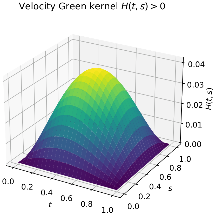
Using the closed form of Proposition 1, the velocity Green kernel H is evaluated on a $401\times 401$ uniform grid. Two checks confirm the theory. First, the closed form (38) agrees with the convolution definition (31) (evaluated by adaptive quadrature to a tolerance of ${10}^{-14}$) to within $1.1\times {10}^{-15}$ at 25 interior sample points, an independent confirmation of Proposition 1. Second, H is strictly positive on the open square, with interior minimum $\approx 2.0\times {10}^{-6}>0$, consistent with Lemma 2. The kernel surface is shown in Figure 1.

7.2. The Interior Cone Estimate and the Optimal Constant

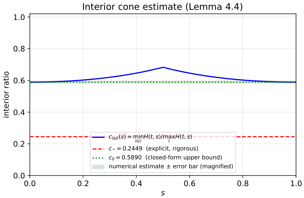
The quantitative interior estimate underlying the refined cone is examined in Figure 2, which plots the ratio $c_{\mathrm{opt}}\left(s\right)$ of Remark 11 against the explicit constant $c_{*}$.

The closed-form endpoint value of Proposition 4 evaluates, for the parameters of Table 1, to

$$c_0={\displaystyle \frac{{min}_{t\in I}\phi \left(t\right)}{{max}_{0\le t\le 1}\phi \left(t\right)}}={\displaystyle \frac{\phi (3/4)}{\phi \left(0.407208\right)}}={\displaystyle \frac{0.06750417}{0.11461377}}=0.588971,$$

so that the optimal uniform constant is enclosed rigorously,

$$0.244921=c_{*}\le c_{\mathrm{sharp}}\le c_0=0.588971.$$

To locate $c_{\mathrm{sharp}}$ inside this interval we also computed ${inf}_s{c}_{\mathrm{opt}}\left(s\right)$ by direct sampling. The estimate obtained is a numerical approximation, and we report it as such together with its sampling density and an a posteriori error bar. Because numerator and denominator of $c_{\mathrm{opt}}$ both vanish like $s(1-s)$ at the endpoints, the sampling is carried out for the desingularized kernel $\widehat{H}(t,s):=H(t,s)/\left(s(1-s)\right)$, which is continuous and strictly positive on ${[0,1]}^2$ and leaves $c_{\mathrm{opt}}$ unchanged.

Table 2. Sampling-density study for ${inf}_s{c}_{\mathrm{opt}}\left(s\right)$ on a uniform $n_s\times n_t$ grid. The values converge monotonically to the closed-form endpoint value $c_0=0.588970856$ of Proposition 4, confirming that the infimum is attained in the endpoint limit.

${\mathit{n}}_{\mathit{s}}={\mathit{n}}_{\mathit{t}}$	Min Over Grid	$|\mathbf{Value}-{\mathit{c}}_0|$
200	0.588992022	$2.12\times {10}^{-5}$
400	0.588973098	$2.24\times {10}^{-6}$
800	0.588971587	$7.31\times {10}^{-7}$
1600	0.588971209	$3.53\times {10}^{-7}$
3200	0.588970889	$3.26\times {10}^{-8}$
6400	0.588970865	$8.97\times {10}^{-9}$
12,800	0.588970859	$3.05\times {10}^{-9}$

shows the effect of refining the sampling grid.

An a posteriori bound is obtained from the Lipschitz data of $\widehat{H}$. On ${[0,1]}^2$ one computes $max|{\partial }_s\widehat{H}|=0.12812$, $max|{\partial }_t\widehat{H}|=0.71954$, ${min}_s{max}_t\widehat{H}=0.12814$ and ${max}_s{min}_{t\in I}\widehat{H}=0.11364$, whence $c_{\mathrm{opt}}$ is Lipschitz with constant $1.887$; with $n_s=n_t=\mathrm{12,800}$ this gives a total error bar of $2.9\times {10}^{-4}$. We therefore report

$${\widehat{c}}_{\mathrm{opt}}=0.5890\pm 2.9\times {10}^{-4}(\mathrm{numerically}\mathrm{estimated}\mathrm{optimal}\mathrm{constant}),$$

which is consistent with the exact value $c_0$ and with the rigorous enclosure. In particular no claim of sharpness rests on the numerics: sharpness of the upper end follows from Proposition 4, and the constant actually used in the theorems is $c_{*}$.

With the uniform weight $a\equiv 1$ (a constant pressure-type drive), the constants of (66) evaluate to

$$M=\underset{0\le t\le 1}{max}{\int }_0^{1}H(t,s)ds=0.0258847,m=\underset{t\in I}{min}{\int }_{1/4}^{3/4}H(t,s)ds=0.0129423,$$

both finite and strictly positive, as required. These were computed with 8-point Gauss–Legendre quadrature on 400 uniform panels, the outer optimization being taken over 2001 values of t.

7.3. A Sufficient Lower Bound on the Load Parameter

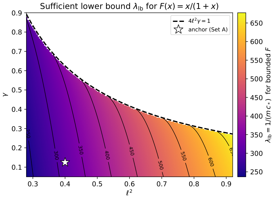
For a bounded nonlinearity the load parameter $\lambda$ is genuinely restricted, which makes the existence conditions physically informative. Taking the saturating law $F\left(x\right)=x/(1+x)$ of Example 3, a positive solution is guaranteed by Theorem 3 once $\lambda m{c}_{*}>1$, i.e., for every

$$\lambda >{\lambda }_{\mathrm{lb}}:={\displaystyle \frac{1}{m{c}_{*}}}.$$

Remark 17

(${\lambda }_{\mathrm{lb}}$ is a sufficient bound, not a critical threshold). The quantity ${\lambda }_{\mathrm{lb}}$ is a sufficient lower bound guaranteeing the existence of a positive solution. It arises from one sufficient fixed-point condition, and nothing in this paper excludes the existence of positive solutions for $\lambda \le {\lambda }_{\mathrm{lb}}$. It is therefore not a critical threshold separating existence from nonexistence, and no sharpness is claimed for it. Establishing a genuine threshold would require a nonexistence result or a bifurcation analysis, which we do not attempt here; results of that type for related higher-order problems may be found in [13,17]. The bound is nevertheless useful precisely because it is computable: it is an explicit function of $({\mathcal{\ell }}^2,\gamma )$.

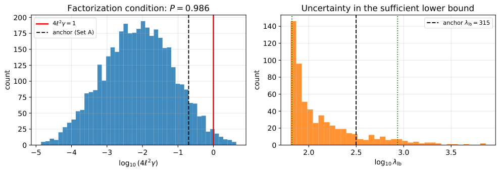
For the anchor parameters, ${\lambda }_{\mathrm{lb}}\approx 315.5$. Figure 3 maps ${\lambda }_{\mathrm{lb}}$ over the admissible portion of the $({\mathcal{\ell }}^2,\gamma )$ plane, bounded by the factorization curve $4{\mathcal{\ell }}^2\gamma =1$. The map admits the following reading, which we record as a numerical observation for the model and parameter range considered, not as a proved monotonicity result: increasing either the couple-stress strength ${\mathcal{\ell }}^2$ or the porous resistance $\gamma$ raises the driving force sufficient to guarantee a positive fully developed profile, and the accessible region shrinks as one approaches the factorization boundary.

Remark 18

(Status of the observed parameter trends). The trends just described, and the suppression of the peak velocity by increasing ${\mathcal{\ell }}^2$ reported in Section 7.6, are observed consistently over the computed range and are physically plausible. They are, however, numerical observations for the specific model, weight $a\equiv 1$ and parameter window used here. We have not proved that ${\lambda }_{\mathrm{lb}}$ is monotone in ${\mathcal{\ell }}^2$ or γ, nor that $\parallel u\parallel$ is monotone in ${\mathcal{\ell }}^2$, and the reader should not read the figures as asserting such a theorem. The distinction matters here because the existence bounds are sufficient and nonsharp (Remark 17).

For a superlinear drive the picture is complementary: with $F\left(x\right)=x^p$, $p>1$, Corollary 1(G1) guarantees a positive solution for every $\lambda >0$, and the admissible radii are explicit. For instance, at $\lambda =50$ and $p=2$ the compression condition (67) holds for $r\le 0.773$ and the expansion condition (68) for $R\ge 25.76$, so the bracket $r<R$ is comfortably realized.

7.4. Numerical Method and Its Verification

This subsection specifies the scheme used to produce Figure 4, Figure 5 and Figure 6 and documents its accuracy. We emphasize once more that the iteration below is a solver: it plays no part in the existence proof, which rests on topological degree rather than on contraction.

7.4.1. Discretization

We solve the fixed-point Equation (50) in the velocity variable,

$$u\left(t\right)=\lambda {\int }_0^{1}H(t,s)a\left(s\right)F\left(u\left(s\right)\right)ds,$$

by a Nyström method. The quadrature nodes are the uniform points $s_j=j/N$, $j=0,\dots ,N$, and the rule is the composite Simpson rule, with weights

$$w_0=w_N=\frac{h}{3},w_j=\frac{4h}{3}\left(j\mathrm{odd}\right),w_j=\frac{2h}{3}(j\mathrm{even},0<j<N),h=\frac{1}{N}.$$

Collocating at the same nodes gives the nonlinear algebraic system

$$u_i=\lambda {\displaystyle \sum _{j=0}^N}{w}_{j}H(t_i,s_j)a\left(s_j\right)F\left(u_j\right),i=0,\dots ,N.$$

(75)

7.4.2. Why Simpson, and Why $N=200$

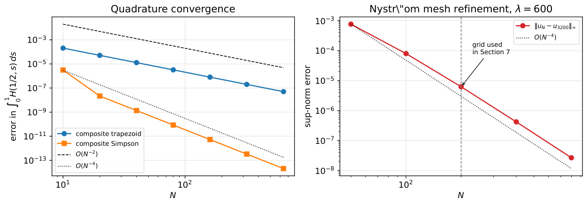
The map $s\mapsto H(t,s)$ is smooth except at $s=t$, where by Lemma 2(iv) the third s-derivative jumps while H, $H_s$ and $H_{ss}$ remain continuous. A jump this weak does not degrade a fourth-order rule.

Table 3. Convergence of the two candidate quadrature rules for ${\int }_0^{1}H(1/2,s)ds$. The reference value $0.0258846808930835$ was obtained by 12-point Gauss–Legendre quadrature on 1000 panels with the interval split at $s=t$.

N	Trapezoid Error	Order	Simpson Error	Order
10	$2.06\times {10}^{-4}$	—	$3.12\times {10}^{-6}$	—
20	$5.14\times {10}^{-5}$	2.00	$2.17\times {10}^{-8}$	7.17
40	$1.29\times {10}^{-5}$	2.00	$1.36\times {10}^{-9}$	4.00
80	$3.22\times {10}^{-6}$	2.00	$8.48\times {10}^{-11}$	4.00
160	$8.04\times {10}^{-7}$	2.00	$5.30\times {10}^{-12}$	4.00
320	$2.01\times {10}^{-7}$	2.00	$3.31\times {10}^{-13}$	4.00
640	$5.02\times {10}^{-8}$	2.00	$2.07\times {10}^{-14}$	4.00

confirms this: the composite trapezoid rule converges at order 2 and composite Simpson at order 4. Simpson is therefore adopted; a further reason is that all its weights are strictly positive, which is what makes the discrete scheme positivity preserving (Section 7.5). With $N=200$, i.e., the 201-point grid used here, the discretization error is $6.2\times {10}^{-6}$ in the sup norm, or $4.4\times {10}^{-7}$ relative with six correct significant digits, far more than the figures require.

7.4.3. Nonlinear Iteration, Starting Value, Stopping Criterion

System (75) is solved by the Picard iteration $u^{(k+1)}=T_N{u}^{\left(k\right)}$, where $T_N$ denotes the right-hand side of (75). The starting approximation is $u^{\left(0\right)}\left(t\right)=0.1sin\left(\pi t\right)$, a nonzero element of the discrete cone. The iteration is stopped when

$${∥u^{(k+1)}-u^{\left(k\right)}∥}_{\infty }<{10}^{-14}.$$

For $\lambda =600$, $F\left(x\right)=x/(1+x)$, $a\equiv 1$ and $N=200$ this is reached in 18 iterations.

7.4.4. Residuals

Two residuals are reported, both for the converged iterate $u_N$:

$$R_{\infty }:={∥u_N-\lambda K_N\left[aF\left(u_N\right)\right]∥}_{\infty },R_2:={\left(\sum _j{w}_j{\left(u_N-\lambda K_N\left[aF\left(u_N\right)\right]\right)}_j^2\right)}^{1/2},$$

where $K_N$ is the discrete Green operator of (75). Their values are

$$R_{\infty }=3.55\times {10}^{-15},R_2=6.59\times {10}^{-16},R_{\infty }/{\parallel u_N\parallel }_{\infty }=2.52\times {10}^{-16},$$

i.e., at the level of double-precision round-off. The value $4\times {10}^{-13}$ quoted in the previous version of this paper referred to the final Picard step, not to a residual; the ambiguity is removed here.

7.4.5. Mesh Refinement

Table 4. Mesh-refinement study for the nonlinear problem at $\lambda =600$, $F\left(x\right)=x/(1+x)$, $a\equiv 1$.

N	Nodes	$\parallel {\mathit{u}}_{\mathit{N}}-{\mathit{u}}_{3200}{\parallel }_{\mathit{\infty }}$	Order	Iterations
50	51	$7.65\times {10}^{-4}$	—	18
100	101	$7.97\times {10}^{-5}$	3.26	18
200	201	$6.25\times {10}^{-6}$	3.67	18
400	401	$4.22\times {10}^{-7}$	3.89	18
800	801	$2.68\times {10}^{-8}$	3.97	18
1600	1601	$1.59\times {10}^{-9}$	4.08	18

reports $\parallel u_N-u_{3200}{\parallel }_{\infty }$ at the coarse nodes. The observed order is 4, consistent with the quadrature analysis.

7.4.6. Independence of the Starting Approximation

Starting from $u^{\left(0\right)}=0.1sin\left(\pi t\right)$, $u^{\left(0\right)}\equiv 1$ and $u^{\left(0\right)}=50sin\left(\pi t\right)$ the iteration reaches the same limit to within $5.3\times {10}^{-15}$, in 18, 17 and 16 iterations respectively. The choice $u^{\left(0\right)}\equiv 0$ is of course excluded: since $F\left(0\right)=0$, the origin is itself a fixed point and the iteration remains there. This is a feature of the problem, not of the solver, and it is one reason the theory works with the cone K and an annulus $\overline{{\Omega }_R}\setminus {\Omega }_r$ rather than with a neighborhood of the origin.

7.4.7. Convergence Mechanism, and What It Does and Does Not Prove

The global Lipschitz bound of the Picard map on the cone is $\lambda M{sup}_{x\ge 0}{F}^{\prime }\left(x\right)=600\times 0.025885\times 1=15.53>1$, so T is not a global contraction and no contraction-mapping argument is available. The observed convergence is instead local: the spectral radius of the discrete Fréchet derivative $T_N^{\prime }\left(u_N\right)=\lambda {\left[w_{j}H(t_i,s_j)a\left(s_j\right)F^{\prime }\left(u_{N,j}\right)\right]}_{i,j}$ at the computed solution is

$$\rho \left(T_N^{\prime }\left(u_N\right)\right)=0.09146,$$

which matches the observed asymptotic linear rate $0.0923$ of the iteration to three digits. Since $\rho <1$, the operator $Id-T_N^{\prime }\left(u_N\right)$ is invertible, so the computed solution is an isolated (locally unique) solution of the discrete system. We stress that this is a statement about the computed solution: the theory of Section 5 establishes existence but neither uniqueness nor multiplicity, and accordingly we refer throughout to a computed positive solution rather than to the solution.

7.4.8. Independent Cross-Check Against the Differential Formulation

As a check that is structurally unrelated to the Nyström scheme, the fourth-order boundary value problem (49) was also solved directly in differential form by Chebyshev collocation with $n=120$ modes and a Newton iteration, imposing $u\left(0\right)=u\left(1\right)=u^{″}\left(0\right)=u^{″}\left(1\right)=0$ exactly through boundary rows. The two solutions agree to

$$\parallel u_{\mathrm{Nyström}}-u_{\mathrm{Chebyshev}}{\parallel }_{\infty }=6.44\times {10}^{-6},\mathrm{relative}4.58\times {10}^{-7},$$

which is the size of the Nyström discretization error at $N=200$ predicted by Table 4. The pointwise residual of the Chebyshev solution in the differential equation, ${\mathcal{\ell }}^2{u}^{\left(4\right)}-u^{″}+\gamma u-\lambda aF\left(u\right)$, is $4.7\times {10}^{-4}$ in absolute value over the interior collocation nodes, i.e., $8.4\times {10}^{-7}$ relative to $\lambda max\left|aF\right(u\left)\right|$.

7.4.9. Boundary Conditions

For the Nyström solution the five boundary conditions of the original fifth-order problem hold identically, not merely to within a tolerance. The reason is structural: the natural Nyström interpolant

$$\tilde{u}\left(t\right):=\lambda {\displaystyle \sum _{j=0}^N}{w}_{j}H(t,s_j)a\left(s_j\right)F\left(u_j\right)$$

(76)

is a finite positive combination of kernel slices $H(·,s_j)$, each of which satisfies $H(0,s)=H(1,s)=0$ and $H_{tt}(0,s)=H_{tt}(1,s)=0$ by Lemma 2(iii). Consequently $\tilde{u}\left(0\right)=\tilde{u}\left(1\right)={\tilde{u}}^{″}\left(0\right)={\tilde{u}}^{″}\left(1\right)=0$, and with $y\left(t\right)={\int }_0^t\tilde{u}$ also $y\left(0\right)=0$, $y^{\prime }\left(0\right)=y^{\prime }\left(1\right)=0$, $y^{″\prime }\left(0\right)=y^{″\prime }\left(1\right)=0$. Numerically all six quantities evaluate to $0.0$ to machine precision. The Chebyshev solution satisfies the same conditions to $2.4\times {10}^{-6}$ or better.

7.5. Positivity of the Computed Solution

The theory predicts $u>0$ on $(0,1)$. Discretization, quadrature, interpolation and iteration could in principle introduce small negative values, and we now show that in this scheme they cannot.

7.5.1. The Discrete Operator Is Exactly Positivity Preserving

All composite Simpson weights are strictly positive (${min}_j{w}_j=h/3=1.67\times {10}^{-3}$ for $N=200$), the kernel satisfies $H(t_i,s_j)\ge 0$, and $a\ge 0$, $F\ge 0$ on $[0,\infty )$. Hence the right-hand side of (75) is an on-negative combination of on-negative terms: the discrete map sends on-negative data to on-negative data exactly, in exact arithmetic and, since no cancellation occurs, in floating point as well. No quadrature-induced negative value is possible. This is the practical reason for preferring Simpson or Gauss–Legendre over any rule with negative weights, such as higher-order Newton–Cotes.

7.5.2. Interpolation Cannot Destroy Positivity Either

Rather than interpolating the nodal values by splines or polynomials, which could undershoot, we use the natural Nyström interpolant (76). For $t\in (0,1)$ each kernel slice $H(t,s_j)$ with $s_j\in (0,1)$ is strictly positive by Lemma 2(i), and the coefficients $w_{j}a\left(s_j\right)F\left(u_j\right)$ are on-negative with at least one strictly positive; therefore $\tilde{u}\left(t\right)>0$ for every$t\in (0,1)$, with no exception and no tolerance. Positivity of the computed profile is thus an identity, not an observation.

7.5.3. Computed Positivity Margin

Evaluating (76) on a 20001-point grid gives

$$\underset{0<t<1}{min}\tilde{u}\left(t\right)=2.25\times {10}^{-3},\underset{0.01\le t\le 0.99}{min}\tilde{u}\left(t\right)=0.4505,\underset{t\in I}{min}\tilde{u}\left(t\right)=10.0347.$$

The first of these is small only because $\tilde{u}$ vanishes at the endpoints, as it must. Subtracting the discretization error of Table 4 from the interior minimum gives the certified bound

$$\underset{t\in I}{min}u\left(t\right)\ge 10.0347-6.3\times {10}^{-6}=10.0347>0,$$

so the positivity margin on the cone interval survives the numerical error by six orders of magnitude.

7.6. A Representative Velocity Field and Its Cone Localization

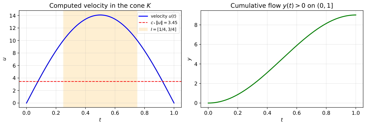
To visualize a solution whose existence is guaranteed by Theorem 3, we solve the velocity problem (49) for the saturating nonlinearity $F\left(x\right)=x/(1+x)$ at $\lambda =600>{\lambda }_{\mathrm{lb}}$ by the scheme documented in Section 7.4. In accordance with Remark 17 and with the local-uniqueness discussion above, what follows is a computed positive solution; the theory does not assert that it is the only one.

The computed velocity field is displayed in Figure 4 together with the interior interval I and the cone level $c_{*}\parallel u\parallel$. The solution satisfies every qualitative prediction of the theory:

• Positivity: $u\left(t\right)>0$ for all $t\in (0,1)$;
• Cone membership: ${min}_{t\in I}u\left(t\right)=10.0347\ge c_{*}\parallel u\parallel =3.4483$, so $u\in K$, with margin $6.5864$;
• The cumulative-flow function $y\left(t\right)={\int }_0^{t}u\left(s\right)ds$ is strictly increasing and strictly positive on $(0,1]$, with $y\left(1\right)=9.0123$, in agreement with the positivity conclusion for the fifth-order problem.

Figure 5 summarizes the two convergence studies of Section 7.4.

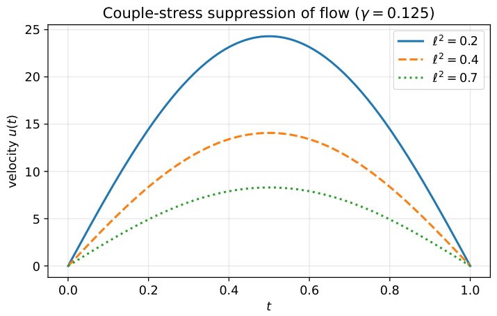
Finally, Figure 6 illustrates the physical role of the couple-stress parameter. Holding $\gamma =0.125$ fixed and increasing ${\mathcal{\ell }}^2$ from $0.2$ to $0.7$, the peak velocity falls from $\parallel u\parallel =24.3041$ through $14.0792$ to $8.3020$: a stiffer microstructure resists deformation and suppresses the throughput, exactly as the couple-stress term ${\eta }_c{U}^{\left(4\right)}$ in the momentum balance (5) would suggest. The theory guarantees a positive solution throughout this range, since all three parameter choices satisfy $4{\mathcal{\ell }}^2\gamma \le 1$ and the corresponding lower-bound condition. As stated in Remark 18, this is a numerical observation over the computed range and not a proved monotonicity result.

7.7. Sensitivity and Uncertainty of the Physical Parameters

Because the values in Table 1 are representative rather than measured (Remark 16), we quantify how the conclusions depend on them. Two complementary analyses are reported.

7.7.1. Local Sensitivity

Table 5. Logarithmic elasticities at the anchor configuration.

	$\mathit{\mu }$	H	${\mathit{\eta }}_{\mathit{c}}$	${\mathit{K}}_{\mathit{p}}$
$c_{*}$	$0.0012$	$-0.0409$	$-0.0012$	$0.0216$
m	$0.7950$	$1.5849$	$-0.7950$	$0.0026$
M	$0.7950$	$1.5849$	$-0.7950$	$0.0026$
${\lambda }_{\mathrm{lb}}$	$-0.7962$	$-1.5441$	$0.7962$	$-0.0242$

gives the logarithmic elasticities $\partial logQ/\partial logp$ of the derived quantities Q with respect to the primitive parameters p, computed by central differences with a relative step ${10}^{-4}$. An entry E means that a $1\%$ increase in p produces approximately an $E\%$ change in Q.

The cone constant $c_{*}$ is remarkably insensitive to all four parameters (every elasticity below $0.05$ in modulus), which is reassuring since $c_{*}$ governs the cone itself. The sufficient bound ${\lambda }_{\mathrm{lb}}$ is dominated by the gap height, with elasticity $-1.54$, and is nearly insensitive to the permeability, with elasticity $-0.024$; the elasticities with respect to $\mu$ and ${\eta }_c$ are equal and opposite, as they must be, since these enter only through ${\eta }_c/\mu$.

7.7.2. Global Uncertainty

A Monte-Carlo study was carried out with 4000 samples drawn log-uniformly from the ranges in the last column of Table 1, each range spanning one to two orders of magnitude around the anchor. The results are:

• The factorization condition $4{\mathcal{\ell }}^2\gamma <1$ holds with probability $0.986$; the 5th, 50th and 95th percentiles of $4{\mathcal{\ell }}^2\gamma$ are $1.7\times {10}^{-4}$, $8.0\times {10}^{-3}$ and $0.334$. The regime required by Assumption 1 is therefore typical rather than exceptional for thin films of this kind;
• Conditional on the condition holding, $c_{*}$ has percentiles $0.117$, $0.246$, $0.250$, so the cone constant is stable across the whole box;
• ${\lambda }_{\mathrm{lb}}$ has percentiles $66.5$, $97.8$, $863.9$, spanning more than an order of magnitude. The anchor value $315.5$ sits at the 85th percentile.

The last item is the practically important one: the sufficient bound is a computable function of the configuration and must be recomputed for each one; it is not a universal number. Figure 7 shows both distributions.

7.7.3. A Second Configuration

Table 6. The anchor configuration and a second configuration inside the conventional squeeze-film range $\mathcal{\ell }\le 0.4$.

Quantity	Symbol	Set A	Set B
Dynamic viscosity	$\mu$	$1.0\times {10}^{-3}$	$1.0\times {10}^{-2}$
Gap height	H	$1.0\times {10}^{-4}$	$5.0\times {10}^{-5}$
Couple-stress coefficient	${\eta }_c$	$4.0\times {10}^{-12}$	$3.0\times {10}^{-12}$
Permeability	$K_p$	$8.0\times {10}^{-8}$	$2.0\times {10}^{-7}$
Couple-stress parameter	${\mathcal{\ell }}^2$	$0.400$	$0.120$
Couple-stress ratio	$\mathcal{\ell }=L_c/H$	$0.632$	$0.346$
Porous-resistance parameter	$\gamma$	$0.125$	$0.0125$
Factorization product	$4{\mathcal{\ell }}^2\gamma$	$0.200$	$0.0060$
Cone constant	$c_{*}$	$0.244921$	$0.249512$
	M	$0.025885$	$0.058644$
	m	$0.012942$	$0.029322$
Sufficient lower bound	${\lambda }_{\mathrm{lb}}$	$315.47$	$136.68$

records a configuration lying inside the couple-stress range conventionally tabulated in squeeze-film studies, $\mathcal{\ell }\le 0.4$. Every qualitative conclusion of this section is unchanged; only the numbers move.

Taken together, these computations show that the assumptions of the existence theorems are satisfied by physically reasonable data, and that the predicted positivity and cone bounds hold in the computed solution. For the chosen parameters, we checked that:

(i)

The operator splits into two factors, with well-separated positive roots $r_1,r_2$;

(ii)

The velocity Green kernel is strictly positive, and its closed form matches the convolution formula to $1.1\times {10}^{-15}$;

(iii)

The cone constant $c_{*}$ is admissible, with the optimal constant enclosed rigorously in $[0.2449,0.5890]$;

(iv)

The sufficient existence condition holds over a clear region of the $({\mathcal{\ell }}^2,\gamma )$ plane, and over $98.6\%$ of a two-decade parameter box;

(v)

A separately computed velocity, verified against an independent differential-equation solver and satisfying all five boundary conditions identically, is positive, stays in the cone, and drops as the couple-stress strength grows.

8. Conclusions

We have studied the fifth-order boundary value problem (4) from fully developed couple-stress flow through a porous channel, a setting that avoids the convective obstacles of stretching-sheet equations while keeping the higher-order couple-stress structure. Under the restriction $0<4{\mathcal{\ell }}^2\gamma \le 1$ the linear velocity operator factorizes into two positive second-order factors, giving a positive velocity kernel H, a non-negative cumulative-flow kernel G, and for $4{\mathcal{\ell }}^2\gamma <1$, the closed form

$$H(t,s)={\displaystyle \frac{g_{r_1}(t,s)-g_{r_2}(t,s)}{\sqrt{1-4{\mathcal{\ell }}^2\gamma }}}.$$

Krasnosel’skiĭ’s theorem then yields positive solutions under elementary conditions on F and $\lambda$, and positivity of the velocity transfers to a strictly positive cumulative flow on $(0,1]$.

A worked application with representative physical parameters confirms these results numerically: the kernel is positive, the explicit cone constant is admissible, and the sufficient existence conditions hold on an identifiable region of the $({\mathcal{\ell }}^2,\gamma )$ plane, where an independently computed velocity field respects the predicted cone bounds.

The numerical part of the paper is documented so as to be reproducible. The integral equation is discretied by a composite-Simpson Nyström scheme whose observed order is four; the computed profile agrees with an independent Chebyshev-collocation solution of the differential formulation to $6.4\times {10}^{-6}$, satisfies all five boundary conditions identically, and is strictly positive at every interior point by construction, since the quadrature weights and the kernel are both positive. Two further by-products of the revision deserve mention. First, the optimal uniform cone constant is enclosed rigorously, $c_{*}\le c_{\mathrm{sharp}}\le c_0$, with both ends given by closed-form elementary expressions (Proposition 4); no claim about it now rests on grid sampling. Second, the structural condition of Assumption 1 is equivalent to the gap-independent comparison of material lengths $2L_c\le \sqrt{K_p}$, and a Monte Carlo study over a two-decade parameter box finds it satisfied with probability $0.986$.

Several questions remain open. The case $4{\mathcal{\ell }}^2\gamma >1$, where the roots are complex and the kernel may change sign, falls outside the present cone framework. The theory gives existence but not uniqueness or multiplicity; numerically the computed solution is isolated, since the spectral radius of the Fréchet derivative there is $0.091<1$, but no global statement follows from this. Establishing whether ${\lambda }_{\mathrm{lb}}=1/\left(m{c}_{*}\right)$ can be improved to a genuine existence/nonexistence threshold, by a nonexistence argument or a bifurcation analysis in the spirit of [13,17], is the most natural next step, as is a proof of the monotonicity in $({\mathcal{\ell }}^2,\gamma )$ that the computations of Section 7.3 suggest but do not establish. And a Forchheimer inertial resistance, entering the momentum balance as an extra term rather than through F, leads to a different operator and a separate analysis.

References

1. Stokes, V.K. Couple stresses in fluids. Phys. Fluids 1966, 9, 1709–1715. [Google Scholar] [CrossRef] [Scilit]
2. Stokes, V.K. Theories of Fluids with Microstructure; Springer: Berlin/Heidelberg, Germany, 1984. [Google Scholar]
3. Agarwal, R.P. Boundary Value Problems for Higher Order Differential Equations; World Scientific: Singapore, 1986. [Google Scholar]
4. Agarwal, R.P.; O’Regan, D.; Wong, P.J.Y. Positive Solutions of Differential, Difference and Integral Equations; Kluwer Academic Publishers: Dordrecht, The Netherlands, 1999. [Google Scholar]
5. Caglar, H.N.; Caglar, S.H.; Twizell, E.H. The numerical solution of fifth-order boundary-value problems with sixth-degree B-spline functions. Appl. Math. Lett. 1999, 12, 25–30. [Google Scholar] [CrossRef] [Scilit]
6. Lamnii, A.; Mraoui, H.; Sbibih, D.; Tijini, A. Sextic spline solution of fifth-order boundary value problems. Math. Comput. Simul. 2008, 77, 237–246. [Google Scholar] [CrossRef] [Scilit]
7. Siddiqi, S.S.; Akram, G. Sextic spline solutions of fifth-order boundary value problems. Appl. Math. Lett. 2007, 20, 591–597. [Google Scholar] [CrossRef] [Scilit]
8. Wazwaz, A.-M. The numerical solution of fifth-order boundary value problems by the decomposition method. J. Comput. Appl. Math. 2001, 136, 259–270. [Google Scholar] [CrossRef] [Scilit]
9. Caglar, H.; Caglar, N. Solution of fifth-order boundary value problems by using local polynomial regression. Appl. Math. Comput. 2007, 186, 952–956. [Google Scholar] [CrossRef] [Scilit]
10. Noor, M.A.; Mohyud-Din, S.T. An efficient algorithm for solving fifth-order boundary value problems. Math. Comput. Model. 2007, 45, 954–964. [Google Scholar] [CrossRef] [Scilit]
11. Odda, S.N. Existence solution for fifth-order differential equations under some conditions. Appl. Math. 2010, 1, 279–282. [Google Scholar]
12. Elhaffaf, A.; Naceri, M. Existence theorems for a fifth-order boundary value problem. J. Math. Syst. Sci. 2014, 4, 1–5. [Google Scholar]
13. Houari, N.; Haddouchi, F. Existence and nonexistence results for fifth-order multipoint boundary value problems involving integral boundary condition. Filomat 2023, 37, 6463–6486. [Google Scholar] [CrossRef] [Scilit]
14. Smirnov, S. Existence of multiple positive solutions for a third-order boundary value problem with nonlocal conditions. Nonlinear Anal. Model. Control 2023, 28, 597–612. [Google Scholar] [CrossRef] [Scilit]
15. Szajnowska, G.; Zima, M. Positive solutions to a third order nonlocal boundary value problem with a parameter. Opusc. Math. 2024, 44, 267–283. [Google Scholar] [CrossRef] [Scilit]
16. Dimitrov, N.D.; Jonnalagadda, J.M. Existence and nonexistence results for a fourth-order boundary value problem with sign-changing Green’s function. Mathematics 2024, 12, 2456. [Google Scholar] [CrossRef] [Scilit]
17. Dimitrov, N.D.; Jonnalagadda, J.M. Existence of three positive solutions for boundary value problem of fourth order with sign-changing Green’s function. Symmetry 2024, 16, 1321. [Google Scholar] [CrossRef] [Scilit]
18. Almuthaybiri, S.; Tisdell, C. Laminar flow in channels with porous walls: Advancing the existence, uniqueness and approximation of solutions via fixed point approaches. J. Fixed Point Theory Appl. 2022, 24, 55. [Google Scholar] [CrossRef] [Scilit]
19. Bekri, Z.; Benaicha, S. Existence of solution for a nonlinear fifth-order three-point boundary value problem. Open J. Math. Anal. 2019, 3, 125–136. [Google Scholar] [CrossRef] [Scilit]
20. Benaicha, S.; Haddouchi, F. Positive solutions of a nonlinear fourth-order integral boundary value problem. An. Univ. West Timiş. Ser. Mat.-Inform. 2016, 54, 73–86. [Google Scholar] [CrossRef] [Scilit][Green Version]
21. Cabada, A.; Precup, R.; Saavedra, L.; Tersian, S.A. Multiple positive solutions to a fourth-order boundary-value problem. Electron. J. Differ. Equ. 2016, 2016, 1–18. [Google Scholar] [CrossRef] [Scilit]
22. Graef, J.R.; Kong, L.; Kong, Q.; Yang, B. Positive solutions to a fourth order boundary value problem. Results Math. 2011, 59, 141–155. [Google Scholar] [CrossRef] [Scilit]
23. Xie, D.; Liu, Y.; Bai, C. Green’s function and positive solutions of a singular nth-order three-point boundary value problem on time scales. Electron. J. Qual. Theory Differ. Equ. 2009, 2009, 1–14. [Google Scholar] [CrossRef] [Scilit]
24. Li, Y. Positive solutions of fourth-order boundary value problems with two parameters. J. Math. Anal. Appl. 2003, 281, 477–484. [Google Scholar] [CrossRef] [Scilit]
25. Bai, Z.; Wang, H. On positive solutions of some nonlinear fourth-order beam equations. J. Math. Anal. Appl. 2002, 270, 357–368. [Google Scholar] [CrossRef] [Scilit]
26. Cid, J.Á.; Franco, D.; Minhós, F. Positive fixed points and fourth-order equations. Bull. Lond. Math. Soc. 2009, 41, 72–78. [Google Scholar] [CrossRef] [Scilit]
27. Ma, T.F. Positive solutions for a beam equation on a nonlinear elastic foundation. Math. Comput. Model. 2004, 39, 1195–1201. [Google Scholar] [CrossRef] [Scilit]
28. Adesanya, S.O.; Kareem, S.O.; Falade, J.A.; Arekete, S.A. Entropy generation analysis for a reactive couple stress fluid flow through a channel saturated with porous material. Energy 2015, 93, 1239–1245. [Google Scholar] [CrossRef] [Scilit]
29. Srinivasacharya, D.; Kaladhar, K. Mixed convection flow of couple stress fluid in a non-Darcy porous medium with Soret and Dufour effects. J. Appl. Sci. Eng. 2012, 15, 415–422. [Google Scholar]
30. Li, X.; Xue, Y.; Dang, F.; Ranjith, P.G.; Xie, H.; Hou, P.; Cai, C. Microscale damage evolution of high-temperature granite under liquid nitrogen thermal shock based on computed tomography analysis. Eng. Geol. 2025, 356, 108274. [Google Scholar] [CrossRef] [Scilit]
31. Xue, Y.; Li, X.; Liu, J.; Ranjith, P.G.; Zhang, Y. Mesoscopic damage enhancement in granite under cyclic liquid nitrogen shocks characterized by computed tomography and texture analysis. Int. J. Rock Mech. Min. Sci. 2025, 194, 106217. [Google Scholar] [CrossRef] [Scilit]
32. Devakar, M.; Sreenivasu, D.; Shankar, B. Analytical solutions of couple stress fluid flows with slip boundary conditions. Alex. Eng. J. 2014, 53, 723–730. [Google Scholar] [CrossRef] [Scilit]
33. Guo, D.; Lakshmikantham, V. Nonlinear Problems in Abstract Cones; Academic Press: Boston, MA, USA, 1988. [Google Scholar]
34. Krasnosel’skiĭ, M.A. Positive Solutions of Operator Equations; Noordhoff: Groningen, The Netherlands, 1964. [Google Scholar]
35. Nield, D.A.; Bejan, A. Convection in Porous Media, 5th ed.; Springer: Cham, Switzerland, 2017. [Google Scholar]
36. Lin, J.-R. Squeeze film characteristics of finite journal bearings: Couple stress fluid model. Tribol. Int. 1998, 31, 201–207. [Google Scholar] [CrossRef] [Scilit]
37. Naduvinamani, N.B.; Siddangouda, A. Squeeze film lubrication between circular stepped plates of couple stress fluids. J. Braz. Soc. Mech. Sci. Eng. 2009, 31, 21–26. [Google Scholar] [CrossRef] [Scilit]
38. Byeon, H.; Latha, Y.L.; Hanumagowda, B.N.; Govindan, V.; Salma, A.; Abdullaev, S.; Tawade, J.V.; Awwad, F.A.; Ismail, E.A.A. Magnetohydrodynamics and viscosity variation in couple stress squeeze film lubrication between rough flat and curved circular plates. Sci. Rep. 2023, 13, 22960. [Google Scholar] [CrossRef] [Scilit]
Figure 1. The velocity Green kernel H ( t , s ) for the parameters of Table 1. The kernel is continuous, symmetric, and strictly positive on ( 0 , 1 ) × ( 0 , 1 ) , in agreement with Lemma 2.
Mathematics 14 03193 g001
Figure 2. Interior cone estimate. For every s ( 0 , 1 ) the ratio c opt ( s ) = min t I H ( t , s ) / max t H ( t , s ) (solid) exceeds the explicit constant c * = 0.2449 (dashed). The dotted line is the closed-form upper bound c 0 = 0.5890 of Proposition 4; the shaded band is the numerical estimate with its error bar, magnified by a factor 20 to be visible. Computed on a 12,800 × 12,800 uniform grid for the desingularized kernel.
Mathematics 14 03193 g002
Figure 3. Sufficient lower bound λ lb = 1 / ( m c * ) for the saturating nonlinearity F ( x ) = x / ( 1 + x ) , over the admissible region 4 2 γ 1 . The dashed curve is the factorization boundary 4 2 γ = 1 ; the star marks the anchor parameters of Table 1. A positive solution is guaranteed for every λ > λ lb ; no claim is made for λ λ lb . Construction:  λ lb was evaluated on a uniform 161 × 161 grid in ( 2 , γ ) [ 0.28 , 0.92 ] × [ 0.05 , 0.90 ] , each evaluation using 8-point Gauss–Legendre quadrature on 60 panels; the color field uses Gouraud shading between grid values and the labeled contours are drawn at the levels shown by matplotlib’s marching-squares algorithm applied to the same grid, with no additional smoothing. Values range from 236.7 to 677.4 over the plotted window.
Mathematics 14 03193 g003
Figure 4. Left: a computed velocity u ( t ) for F ( x ) = x / ( 1 + x ) , λ = 600 . The profile is positive and, on I = [ 1 / 4 , 3 / 4 ] (shaded), lies above the cone level c * u (dashed), confirming u K . Right: the cumulative-flow function y ( t ) = 0 t u , strictly positive on ( 0 , 1 ] . Composite Simpson Nyström scheme, N = 200 .
Mathematics 14 03193 g004
Figure 5. Left: convergence of the composite trapezoid and composite Simpson rules for 0 1 H ( 1 / 2 , s ) d s , with reference slopes. Right: Nyström mesh refinement for the nonlinear problem at λ = 600 , measured against the N = 3200 solution. The vertical line marks the N = 200 grid used in Section 7.6.
Mathematics 14 03193 g005
Figure 6. Effect of couple-stress strength on the velocity profile at fixed porous resistance γ = 0.125 and load λ = 600 . Increasing 2 suppresses the flow, consistent with the resistive character of the couple-stress term. Three computed positive solutions; Nyström, N = 200 .
Mathematics 14 03193 g006
Figure 7. Uncertainty quantification over the parameter ranges of Table 1, 4000 log-uniform samples. Left: distribution of 4 2 γ ; the factorization condition holds with probability 0.986 . Right: distribution of the sufficient lower bound λ lb conditional on the condition holding, with the 5th and 95th percentiles marked.
Mathematics 14 03193 g007