Full Bayesian Analysis of ARX Models Under Scale-Mixtures of Normal Errors: An Application to Solar Radiation in Najran, Saudi Arabia

Abstract

Autoregressive models with exogenous variables (ARX) constitute a fundamental family of time series tools with broad applicability across engineering, environmental science, and finance. A persistent limitation of standard Bayesian treatments is the Gaussian error assumption, which frequently proves inadequate when dealing with real data displaying heavy tails or occasional extreme observations. To overcome this shortcoming, the present paper develops a complete Bayesian inferential framework for ARX models under the scale-mixtures of normal (SMN) error distribution, integrating model identification, parameter estimation, and multi-step-ahead prediction within a unified scheme. A stochastic search variable selection (SSVS) procedure is adapted to perform simultaneous selection of the autoregressive order and the active exogenous regressors by assigning binary latent indicators to each candidate coefficient. Mixture-of-normals priors are specified for the dynamic and exogenous coefficients and an inverse-gamma prior for the error scale, while Bernoulli priors govern the latent selection indicators. These choices yield tractable full conditional posterior distributions: multivariate normal for the complete coefficient vector, inverse-gamma for the scale, and Bernoulli for the indicators. The conditional predictive distribution of future observations is also multivariate normal. For SMN-specific mixing parameters whose conditionals lack standard forms, Metropolis–Hastings steps are embedded within the Gibbs sampler. An extensive simulation study evaluates recovery accuracy across three SMN distributions and several ARX configurations. The methodology is then applied to the forecasting of daily global horizontal irradiance (GHI) in Najran, southwestern Saudi Arabia, using clear-sky GHI as an exogenous covariate, demonstrating the practical value of the proposed framework in a renewable energy context.

1. Introduction

Autoregressive models with exogenous variables (ARX) represent a widely employed class of dynamic models that extend the pure autoregressive (AR) framework by incorporating the explanatory power of observable external covariates. By conditioning the current level of a response variable on its own past values as well as on relevant input signals, ARX models offer a principled and parsimonious representation of a broad range of causal dynamic relationships [1,2]. Their versatility has made them standard tools for prediction and system identification in domains as varied as macroeconomic forecasting [3,4], load and electricity demand modeling [5], environmental science [6], renewable energy systems [7,8], and control engineering [9]. Solar radiation forecasting is a particularly demanding member of this family of applications. Daily global horizontal irradiance (GHI) is strongly driven by a deterministic astronomical envelope, yet the residual day-to-day dynamics are perturbed by intermittent cloud cover, dust intrusions, and other abrupt atmospheric events. These factors induce heavy-tailed, occasionally extreme deviations, while the relevant autoregressive and exogenous lag structure is rarely known in advance. This combination of genuine structural uncertainty and non-Gaussian noise is precisely the joint problem that motivates the present paper. It is revisited throughout as a concrete, substantive application, rather than as a post hoc illustration.

Two distinct inferential problems arise whenever an ARX model is fitted to observed data. The first is structural specification: it is rarely known in advance which AR lags or which external regressor lags carry genuine predictive information [10]. The second is estimation uncertainty: once a structure is tentatively accepted, all parameter uncertainty must be properly propagated to downstream forecasts. Classical methods typically decouple these tasks, resolving structure via information criteria in a first stage and conducting inference conditional on the selected structure in a second stage, thereby ignoring the additional uncertainty stemming from model selection [11]. A fully Bayesian treatment, by contrast, treats model structure and parameter values as jointly uncertain, allowing their posteriors to be learned simultaneously from the data.

The body of Bayesian literature on AR-type models under Gaussian errors is substantial. Foundational regression-based Bayesian inference was laid out by Box and Tiao [12], while Chib and Greenberg [13] introduced a Gibbs sampling approach for regression models with ARMA-correlated disturbances. McCulloch and Tsay [14] demonstrated that full conditional posterior distributions of pure AR models can be expressed in standard forms amenable to direct sampling. The stochastic search variable selection (SSVS) approach of George and McCulloch [15,16] provides a highly effective Bayesian mechanism for variable selection, and its adaptation to time series settings has been pursued by Chen [17], So et al. [18], Chen et al. [19], and Amin et al. [20]. Gibbs sampling has also been proposed for the Bayesian analysis of seasonal ARMA and double-seasonal AR models [21,22]. Bayesian inference for ARX models under Gaussian errors has been pursued along several complementary lines. Peterka [11] derived one of the earliest conjugate posteriors for linear system identification with Gaussian noise, subsuming the ARX model as a special case. Pillonetto et al. [23] later proposed a kernel-based Bayesian framework for regularized system identification in which the ARX structure arises naturally, while Pillonetto and Ljung [24] extended this perspective by treating stable kernels probabilistically and modeling the associated impulse responses as zero-mean Gaussian vectors. More recently, Cooper et al. [10] developed a cross-validation strategy for Bayesian ARX model selection, demonstrating that joint log-scores outperform pointwise criteria under serial dependence.

A complementary concern is the robustness of the assumed error distribution. Departures from Gaussianity—manifesting as excess kurtosis, occasional outliers, or distinct clusters of anomalous observations—are commonplace in environmental, financial, and engineering time series. The scale-mixtures of normal (SMN) distribution [25,26] provide a coherent and flexible way to handle such deviations. By writing each observation as a Gaussian variate with a randomly rescaled variance, the framework subsumes Student’s t, slash, and contaminated normal distributions as members of a common parametric family, while the normal itself arises as a degenerate case. The hierarchical structure of the SMN representation is particularly convenient for Bayesian computation, because conditionally on the latent scale variables, the likelihood is Gaussian, and many full conditional posteriors admit closed forms [27,28].

The intersection of AR modeling and SMN errors has attracted some attention in the literature. Ferreira et al. [29] treated partial linear models with AR disturbances following an SMN distribution, while Mahmoudi et al. [30] considered heavy-tailed finite mixture AR models from a Bayesian viewpoint. Work by Ryu and Kim [31] and Agarwal and Tripathi [32] examined Bayesian inference for pure AR processes under exponential power and Student’s t errors, respectively. Recently, Amin [33,34,35] extended the SMN error framework to seasonal AR models, establishing a full Bayesian estimation, prediction, and analysis procedure. Most recently, Amin and Alghamdi [36] proposed the Bayesian estimation of ARX models under SMN errors. Nevertheless, a comprehensive Bayesian treatment of ARX models under SMN errors—one that integrates simultaneous order and variable selection with robust parameter estimation and multi-step forecasting—appears to be absent from the existing literature.

The present paper fills this gap through several contributions. First, we extend the SSVS mechanism to perform simultaneous selection of AR lags and exogenous variable lags in a general ARX model that is capable of accommodating any number of exogenous inputs with individual lag structures. Second, we derive tractable full conditional posterior distributions for all model unknowns under the SMN assumption. A defining structural feature of the ARX model is its linearity in all coefficients, which permits the joint posterior of the complete coefficient vector to be characterized as a single multivariate normal distribution. Third, we establish a closed-form multivariate normal conditional predictive distribution for multi-step-ahead forecasting, enabling uncertainty-quantified predictions. Fourth, we design a Gibbs sampler with embedded Metropolis–Hastings steps that combines these results into an efficient, fully automated algorithm. Fifth, we validate the methodology via an extensive simulation study and an empirical application to daily solar radiation forecasting in Najran, Saudi Arabia, illustrating the practical utility of the proposed framework in the growing domain of solar energy analytics.

To situate these contributions relative to existing approaches, the proposed framework is positioned against three related strands of the literature: classical (non-Bayesian) ARX modeling [2,37,38], Bayesian ARX under Gaussian errors [10,11,23,24], and robust Bayesian AR-type models under SMN errors that do not address structural selection [29,30,36]. No existing approach combines robust SMN error modeling, joint AR-order and exogenous-lag selection, and closed-form multi-step probabilistic forecasting within a single MCMC sampler, which is the specific gap the present paper closes.

The paper is organized as follows. Section 2 introduces the SMN distribution and presents the ARX model. Section 3 develops the Bayesian framework comprising the SSVS prior structure, the augmented likelihood, the joint posterior, and the predictive formulation. Section 4 derives all full conditional distributions and presents the proposed MCMC algorithm. Section 5 reports the simulation study. Section 6 presents the empirical application to solar radiation in Najran. Section 7 concludes the work.

2. ARX Models Under Scale-Mixtures of Normal Errors

2.1. Scale-Mixtures of Normal Distributions

The SMN class constitutes a rich and analytically tractable family of symmetric distributions capable of representing data with heavier-than-Gaussian tails [25,26]. A scalar random variable y belongs to this class with location $\mu$ and scale parameter ${\sigma }^2$ if it can be expressed as the stochastic mixture:

$$\begin{array}{c}\hfill y=\mu +u^{-1/2}\epsilon ,\end{array}$$

(1)

where $\epsilon \sim N(0,{\sigma }^2)$, the mixing variable $u>0$ has marginal density $p(u\mid \mathit{\nu })$ indexed by a parameter vector $\mathit{\nu }$, and $\epsilon$ and u are mutually independent. Integrating out u gives $y\sim \mathrm{SMN}(\mu ,{\sigma }^2,\mathit{\nu })$, with the conditional distribution $y\mid u\sim N(\mu ,u^{-1}{\sigma }^2)$.

Three SMN special cases are of primary interest. Under $u\sim G(\nu /2,\nu /2)$ with $\nu >0$, the marginal of y is Student’s t with $\nu$ degrees of freedom (SMN-t). When $u\sim \mathrm{Beta}(\nu ,1)$ with $\nu >0$, the resulting distribution is the slash (SMN-sl), which places more probability mass in the tails than the t for moderate $\nu$. Setting u to be a Bernoulli-type variable taking value $\gamma \in (0,1)$ with probability $\nu$ and value 1 with probability $(1-\nu )$, i.e.,

$$\begin{array}{c}\hfill p(u\mid \nu ,\gamma )=\nu {\mathbb{I}}_{\left\{\gamma \right\}}\left(u\right)+(1-\nu ){\mathbb{I}}_{\left\{1\right\}}\left(u\right),\nu ,\gamma \in (0,1),\end{array}$$

(2)

yields the contaminated normal (SMN-cn), a two-component scale mixture capturing occasional large excursions from a dominant Gaussian body. Finally, $p(u=1)=1$ recovers the normal (SMN-n). The SMN family is particularly well-suited to situations where the analyst is uncertain about the degree of tail heaviness, since the mixing parameter $\mathit{\nu }$ can be inferred from the data [27].

2.2. ARX Models

Let $\left\{y_t\right\}$ denote a scalar time series of interest and let $\left\{x_{j,t}\right\}$, $j=1,\dots ,q$, be q observed exogenous sequences. A general ARX model of AR order p, exogenous lag orders $d_1,\dots ,d_q$, and an additive intercept ${\mu }_0$ is defined by:

$$\begin{array}{c}\hfill y_t={\mu }_0+{\displaystyle \sum _{i=1}^p}{\varphi }_i{y}_{t-i}+{\displaystyle \sum _{j=1}^q}{\displaystyle \sum _{l=0}^{d_j-1}}{\alpha }_{jl}{x}_{j,t-l}+{\epsilon }_t,t=1,\dots ,n,\end{array}$$

(3)

where ${\mu }_0$ is the intercept, ${\varphi }_i$ are the AR coefficients, ${\alpha }_{jl}$ is the response coefficient of the l-th lag of the j-th exogenous input, and ${\epsilon }_t$ is an SMN-distributed error with zero mean and scale ${\sigma }^2$. The model intercept ${\mu }_0$ captures the unconditional mean of $y_t$ and guards against bias when the series has a nonzero level, as often occurs after transformations such as differencing or log-ratio computation.

Remark 1.

Standard sub-models follow immediately from (3). Removing all exogenous inputs ($q=0$) gives the AR$\left(p\right)$ model. Removing the AR component ($p=0$) and keeping $d_j=1$ yields the multiple linear regression model.

To express the model compactly, define the augmented regressor vector

$$\begin{array}{c}\hfill {\mathit{z}}_t={\left(1,y_{t-1},\dots ,y_{t-p},x_{1,t},\dots ,x_{1,t-d_1+1},\dots ,x_{q,t},\dots ,x_{q,t-d_q+1}\right)}^T,\end{array}$$

(4)

and the full coefficient vector

$$\begin{array}{c}\hfill \mathit{\theta }={\left({\mu }_0,{\varphi }_1,\dots ,{\varphi }_p,{\alpha }_{10},\dots ,{\alpha }_{1,d_1-1},\dots ,{\alpha }_{q0},\dots ,{\alpha }_{q,d_q-1}\right)}^T,\end{array}$$

(5)

of dimension $m=1+p+{\sum }_{j=1}^q{d}_j$. The model then reads

$$\begin{array}{c}\hfill y_t={\mathit{z}}_t^T\mathit{\theta }+{\epsilon }_t,\end{array}$$

(6)

and stacking all n observations yields the matrix form

$$\begin{array}{c}\hfill \mathit{y}=\mathit{Z}\mathit{\theta }+\mathit{\epsilon },\end{array}$$

(7)

where $\mathit{y}={(y_1,\dots ,y_n)}^T$, $\mathit{\epsilon }={({\epsilon }_1,\dots ,{\epsilon }_n)}^T$, and $\mathit{Z}$ is the $n\times m$ design matrix with t-th row ${\mathit{z}}_t^T$. The matrix $\mathit{Z}$ partitions naturally as

$$\begin{array}{c}\hfill \mathit{Z}=\left[{\mathbf{1}}_n\left|{\mathit{Y}}_L\right|{\mathit{X}}_1|\cdots |{\mathit{X}}_q\right],\end{array}$$

(8)

where ${\mathbf{1}}_n$ is the n-vector of ones corresponding to the intercept, ${\mathit{Y}}_L$ is the $n\times p$ lag matrix with $(t,i)$-entry $y_{t-i}$, and ${\mathit{X}}_j$ is the $n\times d_j$ matrix with $(t,l)$-entry $x_{j,t-l}$.

A key structural property of the ARX model that will be central to the Bayesian derivations is its linearity in $\mathit{\theta }$. Because ${\mathit{z}}_t$ contains only predetermined quantities (past observations and current/past exogenous values) and the intercept is a constant, the conditional mean ${\mathit{z}}_t^T\mathit{\theta }$ is linear in $\mathit{\theta }$ for all t. In the present ARX setting, linearity enables the full conditional posterior of the entire augmented coefficient vector $\mathit{\theta }$—encompassing intercept, AR lags, and all exogenous regressors—to be obtained analytically as a multivariate normal distribution, as shown later in Section 4.

An inferential challenge persists even for this linear model. The values of p and $d_1,\dots ,d_q$ are typically unknown. We handle this by fixing upper bounds $p_{max}$ and $d_{j,max}$ and relying on the SSVS to select active elements [15].

3. Bayesian Framework

3.1. Prior Specification

For each coefficient ${\theta }_k$, $k=1,\dots ,m$, we introduce a binary latent indicator ${\delta }_k\in \{0,1\}$, where ${\delta }_k=1$ signifies that the k-th regressor is active and ${\delta }_k=0$ that it is negligible. Following George and McCulloch [15], the conditional prior on ${\theta }_k$ given ${\delta }_k$ is a two-component normal mixture:

$$\begin{array}{c}\hfill \zeta ({\theta }_k\mid {\delta }_k)={\delta }_{k}N(0,c_k^2{\tau }_k^2)+(1-{\delta }_k)N(0,{\tau }_k^2),k=1,\dots ,m.\end{array}$$

(9)

Here, ${\tau }_k^2\ll 1$ concentrates ${\theta }_k$ near zero when the regressor is excluded, while $c_k^2{\tau }_k^2$ with $c_k\gg 1$ allows ${\theta }_k$ to be appreciably different from zero when the regressor is included. Conditional independence of the ${\theta }_k$’s given their indicators leads to the multivariate normal prior:

$$\begin{array}{c}\hfill \zeta (\mathit{\theta }\mid \mathit{\delta })=N_m\left(\mathbf{0},{\mathit{M}}_{\delta }\mathit{W}{\mathit{M}}_{\delta }\right),\end{array}$$

(10)

where ${\mathit{M}}_{\delta }=\mathrm{diag}(a_1{\tau }_1,\dots ,a_m{\tau }_m)$ with $a_k=c_k$ if ${\delta }_k=1$ and $a_k=1$ otherwise, and $\mathit{W}$ is a prior correlation matrix.

For the error scale parameter, an inverse-gamma prior is adopted:

$$\begin{array}{c}\hfill \zeta \left({\sigma }^2\right)=IG\left(\frac{a_0}{2},\frac{b_0}{2}\right),\end{array}$$

(11)

where $a_0,b_0>0$ are hyperparameters; small values make the prior diffuse. Each latent indicator independently follows a Bernoulli prior $p({\delta }_k=1)=P_k$, and the joint prior over $\mathit{\delta }={({\delta }_1,\dots ,{\delta }_m)}^T$ is:

$$\begin{array}{c}\hfill \zeta \left(\mathit{\delta }\right)={\displaystyle \prod _{k=1}^m}{P}_k^{{\delta }_k}{(1-P_k)}^{1-{\delta }_k}.\end{array}$$

(12)

Equal prior inclusion probabilities $P_k=1/2$ yield the non-informative uniform prior $\zeta \left(\mathit{\delta }\right)=2^{-m}$ over all $2^m$ submodels. Priors for $\mathit{\nu }$ follow Cabral et al. [28]. SMN-t uses a truncated exponential on $\nu \in (2,\infty )$ with rate parameter $\lambda \sim U(c,d)$, SMN-sl uses the same but on $\nu \in (1,\infty )$, and SMN-cn uses $\nu \sim \mathrm{Beta}({\nu }_0,{\nu }_1)$ and $\gamma \sim \mathrm{Beta}({\gamma }_0,{\gamma }_1)$.

Hyperparameter configuration. Following the recommendations of George and McCulloch [15] for the SSVS prior (9), the spike variance is set small, ${\tau }_k^2=0.01$, and the slab-to-spike variance ratio is set large, $c_k^2=100$, for every candidate coefficient ${\theta }_k$, so that excluded regressors are shrunk close to zero while included regressors are essentially unconstrained relative to the scale of the data. The prior inclusion probabilities are set to $P_k=0.5$, corresponding to the non-informative uniform prior over all $2^m$ candidate submodels discussed above. The error-scale prior is set diffuse, $a_0=b_0=0.01$, so that $\zeta \left({\sigma }^2\right)$ contributes negligible prior information relative to the likelihood. These default choices are adopted in this work, while a sensitivity analysis of the ARX-SMN posterior with respect to alternative specifications of $(c_k,{\tau }_k,a_0,b_0)$ represents a worthwhile extension that is left for future research. Accordingly, the variable-selection outcomes and posterior summaries reported in Section 5 and Section 6 should be interpreted as conditional on this hyperparameter configuration. A different, yet still reasonable, choice of $(c_k,{\tau }_k,a_0,b_0)$ could shift individual inclusion probabilities and posterior interval widths. Even so, the broad substantive conclusions are expected to remain robust, given how far these estimates lie from zero relative to their posterior spread.

Collecting $\Theta =(\mathit{\theta },{\sigma }^2,\mathit{\delta },\mathit{\nu })$ and assuming $(\mathit{\theta },{\sigma }^2,\mathit{\delta })\perp \mathit{\nu }$ a priori, the joint prior factorizes as:

$$\begin{array}{c}\hfill \zeta (\Theta )=\zeta (\mathit{\theta }\mid \mathit{\delta })\zeta \left({\sigma }^2\right)\zeta \left(\mathit{\delta }\right)\zeta \left(\mathit{\nu }\right).\end{array}$$

(13)

3.2. Augmented Likelihood and Joint Posterior

Let $\mathit{u}={(u_1,\dots ,u_n)}^T$ collect the latent scale variables. Conditional on $\mathit{u}$, each error ${\epsilon }_t\mid u_t\sim N(0,u_t^{-1}{\sigma }^2)$, so from the SMN representation (1) and model (6), $y_t\mid \mathit{\theta },{\sigma }^2,u_t\sim N({\mathit{z}}_t^T\mathit{\theta },u_t^{-1}{\sigma }^2)$ with density

$$\begin{array}{c}\hfill \zeta (y_t\mid \mathit{\theta },{\sigma }^2,u_t)={\left({\displaystyle \frac{u_t}{2\pi {\sigma }^2}}\right)}^{1/2}exp\left\{-{\displaystyle \frac{u_t}{2{\sigma }^2}}{(y_t-{\mathit{z}}_t^T\mathit{\theta })}^2\right\}.\end{array}$$

Because the ${\epsilon }_t$ are conditionally independent across $t=1,\dots ,n$, and each $u_t$ is independent of $\mathit{\theta },{\sigma }^2$ a priori with density $p(u_t\mid \mathit{\nu })$, the augmented joint density of $(\mathit{y},\mathit{u})$ is obtained by multiplying $\zeta (y_t\mid \mathit{\theta },{\sigma }^2,u_t)$ and $p(u_t\mid \mathit{\nu })$ over t. Since each $u_t$ enters its own summand only as a scalar weight on the corresponding squared residual ${(y_t-{\mathit{z}}_t^T\mathit{\theta })}^2$, the n individual exponents stack into the single quadratic form ${(\mathit{y}-\mathit{Z}\mathit{\theta })}^T\mathit{U}(\mathit{y}-\mathit{Z}\mathit{\theta })$, with $\mathit{U}=\mathrm{diag}(u_1,\dots ,u_n)$ collecting the weights. This gives

$$\begin{array}{c}\hfill \zeta (\mathit{y},\mathit{u}\mid \mathit{\theta },{\sigma }^2,\mathit{\nu })\propto {\left({\sigma }^2\right)}^{-n/2}exp\left\{-{\displaystyle \frac{1}{2{\sigma }^2}}{(\mathit{y}-\mathit{Z}\mathit{\theta })}^T\mathit{U}(\mathit{y}-\mathit{Z}\mathit{\theta })\right\}{\displaystyle \prod _{t=1}^n}{u}_t^{1/2}p(u_t\mid \mathit{\nu }).\end{array}$$

(14)

Equation (14) is a standard hierarchical data-augmentation device for SMN distributions [27,28]. Conditioning on $\mathit{u}$ gives a weighted-least-squares Gaussian kernel with observation-specific precisions $u_t/{\sigma }^2$, while marginalizing over $\mathit{u}$ recovers the (non-Gaussian) SMN likelihood. Applying Bayes’ theorem with the joint prior (13) yields the joint posterior

$$\begin{array}{c}\hfill \zeta (\mathit{\theta },{\sigma }^2,\mathit{\delta },\mathit{u},\mathit{\nu }\mid \mathit{y})\propto \zeta (\Theta ){\left({\sigma }^2\right)}^{-n/2}exp\left\{-{\displaystyle \frac{1}{2{\sigma }^2}}{(\mathit{y}-\mathit{Z}\mathit{\theta })}^T\mathit{U}(\mathit{y}-\mathit{Z}\mathit{\theta })\right\}{\displaystyle \prod _{t=1}^n}{u}_t^{1/2}p(u_t\mid \mathit{\nu }).\end{array}$$

(15)

Since $\mathit{Z}\mathit{\theta }$ is linear in $\mathit{\theta }$, the exponent in (15) is a negative definite quadratic form in $\mathit{\theta }$, guaranteeing a Gaussian conditional posterior for $\mathit{\theta }$ as established in Section 4.1.

3.3. Predictive Formulation

Let ${\mathit{y}}_f={(y_{n+1},\dots ,y_{n+k})}^T$ be the vector of k future observations. The h-step-ahead equation is

$$\begin{array}{c}\hfill y_{n+h}={\mathit{z}}_{n+h}^T\mathit{\theta }+{\epsilon }_{n+h},h=1,\dots ,k,\end{array}$$

(16)

where ${\mathit{z}}_{n+h}$ includes the intercept indicator, AR terms (drawing on future y’s for $h>1$), and the future exogenous values assumed known or externally projected. Expressing the k future equations jointly in matrix notation,

$$\begin{array}{c}\hfill {\mathit{y}}_f={\mathit{Z}}_f^{-1}\left({\mathit{W}}_f{\mathit{y}}_L+{\mathit{X}}_f^{\ast }\mathit{\alpha }+{\mu }_0{\mathit{c}}_f\right)+{\mathit{Z}}_f^{-1}{\mathit{\epsilon }}_f,\end{array}$$

(17)

where ${\mathit{Z}}_f$ is the $k\times k$ lower-triangular AR recursion matrix, ${\mathit{W}}_f$ carries the AR weights applied to the last p observed values ${\mathit{y}}_L={(y_n,\dots ,y_{n-p+1})}^T$, ${\mathit{X}}_f^{\ast }$ collects the future exogenous values weighted by $\mathit{\alpha }$, ${\mathit{c}}_f$ absorbs the cumulative intercept contributions, and ${\mathit{\epsilon }}_f={({\epsilon }_{n+1},\dots ,{\epsilon }_{n+k})}^T$ are the future errors. The unconditional predictive density $\zeta ({\mathit{y}}_f\mid \mathit{y})$ is obtained by marginalizing the conditional predictive distribution over the joint posterior (15). As shown next, the conditional predictive distribution is multivariate normal, enabling efficient Monte Carlo approximation via the MCMC algorithm.

4. Conditional Distributions and MCMC Algorithm

4.1. Full Conditional Posterior and Predictive Distributions

At this stage, we derive the full collection of conditional distributions that serve as the foundation for the MCMC algorithm in Bayesian analysis of ARX models.

4.1.1. Conditional Posterior of $\mathit{\theta }$

Retaining only the terms in (15) that depend on $\mathit{\theta }$ and using the multivariate normal prior (10), we obtain the kernel

$$\begin{array}{c}\hfill \zeta (\mathit{\theta }\mid {\sigma }^2,\mathit{\delta },\mathit{u},\mathit{\nu },\mathit{y})\propto exp\left\{-{\displaystyle \frac{1}{2{\sigma }^2}}{(\mathit{y}-\mathit{Z}\mathit{\theta })}^T\mathit{U}(\mathit{y}-\mathit{Z}\mathit{\theta })-{\displaystyle \frac{1}{2}}{\mathit{\theta }}^T{\Sigma }_0^{-1}\left(\mathit{\delta }\right)\mathit{\theta }\right\},\end{array}$$

(18)

where ${\Sigma }_0\left(\mathit{\delta }\right)$ is the prior covariance matrix $\left({\mathit{M}}_{\delta }\mathit{W}{\mathit{M}}_{\delta }\right)$ for the model coefficients. Expanding the exponent gives $-\frac{1}{2}\left[{\mathit{\theta }}^T\left({\sigma }^{-2}{\mathit{Z}}^T\mathit{U}\mathit{Z}+{\Sigma }_0^{-1}\left(\mathit{\delta }\right)\right)\mathit{\theta }-2{\sigma }^{-2}{\mathit{\theta }}^T{\mathit{Z}}^T\mathit{U}\mathit{y}\right]+\mathrm{const}$, a quadratic form in $\mathit{\theta }$ whose leading matrix is the posterior precision. Matching this to the canonical form $-\frac{1}{2}{(\mathit{\theta }-{\mathit{\mu }}_{\theta }^{\ast })}^T{\left({\mathit{V}}_{\theta }^{\ast }\right)}^{-1}(\mathit{\theta }-{\mathit{\mu }}_{\theta }^{\ast })$ of a Gaussian density—i.e., completing the square in $\mathit{\theta }$—yields the multivariate normal $N_m({\mathit{\mu }}_{\theta }^{\ast },{\mathit{V}}_{\theta }^{\ast })$, with 

$$\begin{array}{c}\hfill {\mathit{V}}_{\theta }^{\ast }={\sigma }^2{\left({\mathit{Z}}^T\mathit{U}\mathit{Z}+{\sigma }^{-2}{\Sigma }_0^{-1}\left(\mathit{\delta }\right)\right)}^{-1},{\mathit{\mu }}_{\theta }^{\ast }={\displaystyle \frac{1}{{\sigma }^2}}{\mathit{V}}_{\theta }^{\ast }{\mathit{Z}}^T\mathit{U}\mathit{y}.\end{array}$$

(19)

This is the usual conjugate update of a Gaussian likelihood (14) with a Gaussian prior (10), so no further approximation is required at this step.

4.1.2. Conditional Posterior of ${\sigma }^2$

Since $(\mathit{\theta },\mathit{\delta })$ enter (14) only through $\mathit{\theta }$, this term is fixed when conditioning on $\mathit{\theta }$, and the augmented likelihood contributes the kernel ${\left({\sigma }^2\right)}^{-n/2}exp\{-Q/\left(2{\sigma }^2\right)\}$ with $Q={(\mathit{y}-\mathit{Z}\mathit{\theta })}^T\mathit{U}(\mathit{y}-\mathit{Z}\mathit{\theta })$, which is conjugate to the inverse-gamma prior (11). Collecting only the ${\sigma }^2$-dependent terms from (15) identifies an inverse-gamma kernel:

$$\begin{array}{c}\hfill {\sigma }^2\mid \mathrm{rest}\sim IG\left(\frac{a_0+n}{2},\frac{b_0+{(\mathit{y}-\mathit{Z}\mathit{\theta })}^T\mathit{U}(\mathit{y}-\mathit{Z}\mathit{\theta })}{2}\right).\end{array}$$

(20)

i.e., the prior shape $a_0/2$ and rate $b_0/2$ are updated by adding half the sample size and half the weighted residual sum of squares Q, respectively the standard normal-inverse-gamma conjugate pairing.

4.1.3. Conditional Posterior of Each ${\delta }_k$

Since ${\delta }_k$ enters the model only through the two-component mixture prior (9) on ${\theta }_k$, Bayes’ rule applied to the discrete prior $\{P_k,1-P_k\}$ on ${\delta }_k=\{1,0\}$, weighted by the conditional density of ${\theta }_k$ under the corresponding mixture component, gives $p({\delta }_k=1\mid {\theta }_k,\mathrm{rest})\propto P_k\zeta ({\theta }_k\mid {\delta }_k=1,\mathrm{rest})$ and $p({\delta }_k=0\mid {\theta }_k,\mathrm{rest})\propto (1-P_k)\zeta ({\theta }_k\mid {\delta }_k=0,\mathrm{rest})$; normalizing these two quantities to sum to one shows that for each $k=1,\dots ,m$, the conditional posterior of ${\delta }_k$ is Bernoulli with inclusion probability

$$\begin{array}{c}\hfill p({\delta }_k=1\mid \mathit{\theta },{\sigma }^2,{\mathit{\delta }}_{(-k)},\mathit{u},\mathit{\nu },\mathit{y})={\displaystyle \frac{A_k}{A_k+B_k}},\end{array}$$

(21)

where $A_k=P_k\zeta ({\theta }_k\mid {\delta }_k=1,\mathrm{rest})$ and $B_k=(1-P_k)\zeta ({\theta }_k\mid {\delta }_k=0,\mathrm{rest})$. This posterior-odds update is the standard two-component mixture computation underlying the SSVS mechanism of George and McCulloch [15].

4.1.4. Conditional Posteriors Under SMN-t

The conditional posterior of each scale variable $u_t$ is a gamma distribution:

$$\begin{array}{c}\hfill u_t\mid \mathrm{rest}\sim G\left({\displaystyle \frac{\nu +1}{2}},{\displaystyle \frac{{(y_t-{\mathit{z}}_t^T\mathit{\theta })}^2}{2{\sigma }^2}}+{\displaystyle \frac{\nu }{2}}\right).\end{array}$$

(22)

This follows because, with $e_t=y_t-{\mathit{z}}_t^T\mathit{\theta }$, the augmented likelihood (14) contributes the factor $u_t^{1/2}exp\{-u_t{e}_t^2/\left(2{\sigma }^2\right)\}$, and the SMN-t mixing density is $u_t\sim G(\nu /2,\nu /2)$; multiplying the two gives a kernel proportional to $u_t^{(\nu +1)/2-1}exp\{-u_t[e_t^2/\left(2{\sigma }^2\right)+\nu /2]\}$, which is recognized directly as the Gamma density in (22)—again a direct conjugacy result requiring no approximation.

The degrees-of-freedom parameter $\nu$ has a non-standard conditional posterior:

$$\begin{array}{c}\hfill \zeta (\nu \mid \mathrm{rest})\propto {\left({\displaystyle \frac{{(\nu /2)}^{\nu /2}}{\Gamma (\nu /2)}}\right)}^n{\displaystyle \prod _{t=1}^n}{u}_t^{\nu /2-1}exp\left\{-\nu \left(\frac{1}{2}{\sum }_{t=1}^n{u}_t+\lambda \right)\right\},\nu >2,\end{array}$$

(23)

sampled via a Metropolis–Hastings step using the truncated normal proposal:

$$\begin{array}{c}\hfill TN\left({\nu }^{(i-1)}-c_{\nu }/d_{\nu },\sqrt{-1/d_{\nu }},(2,\infty )\right),\end{array}$$

(24)

where $c_{\nu }$ and $d_{\nu }$ are the first and second derivatives of $log\zeta (\nu \mid ·)$ evaluated at ${\nu }^{(i-1)}$. The candidate is accepted with probability $min\{r,1\}$, where r is given as:

$$\begin{array}{cc}\hfill r& =\left[\zeta ({\nu }^{\ast }\mid ·)f({\nu }^{(i-1)}\mid {\nu }^{\ast },·)\right]/\left[\zeta ({\nu }^{(i-1)}\mid ·)f({\nu }^{\ast }\mid {\nu }^{(i-1)},·)\right].\end{array}$$

(25)

The hyperparameter $\lambda$ follows $\lambda \mid \nu \sim TG(2,\nu ,(c,d\left)\right)$.

4.1.5. Conditional Posteriors Under SMN-sl

The conditional posterior of each scale variable $u_t$ is a truncated gamma distribution:

$$\begin{array}{c}\hfill u_t\mid \mathrm{rest}\sim TG\left(\nu +{\displaystyle \frac{1}{2}},{\displaystyle \frac{{(y_t-{\mathit{z}}_t^T\mathit{\theta })}^2}{2{\sigma }^2}},(0,1)\right).\end{array}$$

(26)

This is obtained, as for SMN-t above, by multiplying the same Gaussian-kernel factor $u_t^{1/2}exp\{-u_t{e}_t^2/\left(2{\sigma }^2\right)\}$ by the slash mixing density $p(u_t\mid \nu )\propto u_t^{\nu -1}{\mathbb{1}}_{(0,1)}\left(u_t\right)$ and recognizing the resulting kernel as a Gamma density truncated to $(0,1)$. The $\nu$ has a truncated gamma distribution:

$$\begin{array}{c}\hfill \nu \mid \mathrm{rest}\sim TG\left(n+1,\lambda -{\displaystyle \sum _{t=1}^n}log{u}_t,(1,\infty )\right),\end{array}$$

(27)

and the hyperparameter $\lambda$ follows $\lambda \mid \nu \sim TG(2,\nu ,(c,d\left)\right)$.

4.1.6. Conditional Posteriors Under SMN-cn

Because the SMN-cn mixing variable takes only the two values $\{\gamma ,1\}$ with prior weights $\{\nu ,1-\nu \}$ (2), multiplying each prior weight by the corresponding Gaussian-kernel factor from (14) and renormalizing gives a discrete (two-point) conditional posterior for $u_t$. Specifically, the scale variable $u_t$ follows the two-point distribution taking value $\gamma$ with weight ${\nu }_1^{\ast }/({\nu }_1^{\ast }+{\nu }_2^{\ast })$ and value 1 with weight ${\nu }_2^{\ast }/({\nu }_1^{\ast }+{\nu }_2^{\ast })$, where

$$\begin{array}{c}\hfill {\nu }_1^{\ast }=\nu {\gamma }^{1/2}exp\left\{-\frac{\gamma }{2{\sigma }^2}{(y_t-{\mathit{z}}_t^T\mathit{\theta })}^2\right\},{\nu }_2^{\ast }=(1-\nu )exp\left\{-\frac{1}{2{\sigma }^2}{(y_t-{\mathit{z}}_t^T\mathit{\theta })}^2\right\}.\end{array}$$

(28)

The contamination weight satisfies $\nu \mid \mathrm{rest}\sim \mathrm{Beta}({\nu }_0+m_{\gamma },{\nu }_1+n-m_{\gamma })$, with $m_{\gamma }={\sum }_t\mathbb{1}(u_t=\gamma )$. The contamination severity parameter $\gamma$ has the non-standard conditional posterior

$$\begin{array}{c}\hfill \zeta (\gamma \mid \mathrm{rest})\propto {\gamma }^{{\gamma }_0-1}{(1-\gamma )}^{{\gamma }_1-1}{\displaystyle \prod _{t=1}^n}\left[\nu {\gamma }^{1/2}{e}^{-{\displaystyle \frac{\gamma }{2{\sigma }^2}}{(y_t-{\mathit{z}}_t^T\mathit{\theta })}^2}+(1-\nu )e^{-{\displaystyle \frac{1}{2{\sigma }^2}}{(y_t-{\mathit{z}}_t^T\mathit{\theta })}^2}\right],\end{array}$$

(29)

sampled with a Metropolis–Hastings step using the logit-normal proposal.

4.1.7. Conditional Predictive Distribution of ${\mathit{y}}_f$

Since (17) expresses ${\mathit{y}}_f$ as an affine transformation of the future error vector ${\mathit{\epsilon }}_f$, and ${\mathit{\epsilon }}_f\mid {\mathit{U}}_f,{\sigma }^2$ is jointly Gaussian under the same SMN hierarchy introduced in Section 3.2, it follows that any affine transformation of a Gaussian vector is itself Gaussian. Expanding (17) and marginalizing over all quantities other than ${\mathit{y}}_f$, the conditional predictive distribution is multivariate normal $N_k({\mathit{\mu }}_{y_f}^{\ast },{\mathit{V}}_{y_f}^{\ast })$, where

$$\begin{array}{c}\hfill {\mathit{\mu }}_{y_f}^{\ast }={\mathit{Z}}_f^{-1}\left({\mathit{W}}_f{\mathit{y}}_L+{\mathit{X}}_f^{\ast }\mathit{\alpha }+{\mu }_0{\mathit{c}}_f\right),{\mathit{V}}_{y_f}^{\ast }={\sigma }^2{\left[{\mathit{Z}}_f^T{\mathit{U}}_f{\mathit{Z}}_f\right]}^{-1},\end{array}$$

(30)

with ${\mathit{U}}_f=\mathrm{diag}(u_{n+1},\dots ,u_{n+k})$, and the recursion matrices

$${\mathit{Z}}_f={\left(\begin{array}{cccc}1& 0& \dots & 0\\ -{\varphi }_1& 1& \dots & 0\\ ⋮& \ddots & \ddots & ⋮\\ -{\varphi }_{k-1}& \dots & -{\varphi }_1& 1\end{array}\right)}_{k\times k},{\mathit{W}}_f={\left(\begin{array}{cccc}{\varphi }_1& {\varphi }_2& \dots & {\varphi }_p\\ {\varphi }_2& {\varphi }_3& \dots & 0\\ ⋮& & \ddots & ⋮\\ {\varphi }_k& \dots & {\varphi }_p& 0\end{array}\right)}_{k\times p}.$$

4.2. MCMC Algorithm for Full Bayesian Analysis of ARX Models

The full conditional posterior distributions derived in the preceding subsections, alongside the conditional predictive distribution, collectively provide all the necessary building blocks for constructing an efficient MCMC algorithm that carries out the full Bayesian analysis on the ARX model under SMN errors. This MCMC algorithm encompasses identification, estimation, and multi-step-ahead forecasting within a single algorithmic pass. These distributions are now assembled into the Gibbs sampler with embedded Metropolis–Hastings steps presented in Algorithm 1.

Algorithm 1 MCMC algorithm for full Bayesian analysis of ARX-SMN Models

1: Inputs: Observations $\mathit{y}$; exogenous matrices ${\mathit{X}}_1,\dots ,{\mathit{X}}_q$; upper bounds $p_{max}$, $d_{j,max}$; forecast horizon k; future exogenous values; MCMC settings $N_{\mathrm{sim}}$, $N_{\mathrm{burn}}$, $N_{\mathrm{thin}}$. 2: Construct $\mathit{Z}$ via (8). Initialize ${\mathit{\theta }}^{\left(0\right)}$ and ${\left({\sigma }^2\right)}^{\left(0\right)}$ using OLS on the full model. 3: for  $r=1,\dots ,N_{\mathrm{sim}}$do 4:        ${\mathit{\theta }}^{\left(r\right)}\sim N_m({\mathit{\mu }}_{\theta }^{\ast },{\mathit{V}}_{\theta }^{\ast })$                             [Equation (19)] 5:        ${\left({\sigma }^2\right)}^{\left(r\right)}\sim IG\left(\frac{a_0+n}{2},\frac{b^{\ast }}{2}\right)$                           [Equation (20)] 6:        ${\delta }_k^{\left(r\right)}\sim \mathrm{Bin}(1,A_k/(A_k+B_k))$, $k=1,\dots ,m$                     [Equation (21)] 7:        ${\mathit{y}}_f^{\left(r\right)}\sim N_k({\mathit{\mu }}_{y_f}^{\ast },{\mathit{V}}_{y_f}^{\ast })$                            [Equation (30)] 8:        SMN-specific steps: 9:          SMN-t:      $u_t^{\left(r\right)}\sim G\left(\frac{\nu +1}{2},\frac{{(y_t-{\mathit{z}}_t^T\mathit{\theta })}^2}{2{\sigma }^2}+\frac{\nu }{2}\right)$$\forall t$;      ${\nu }^{\left(r\right)}$: MH from (23)–(24);      ${\lambda }^{\left(r\right)}\sim TG(2,\nu ,(c,d))$ 10:        SMN-sl:    $u_t^{\left(r\right)}\sim TG\left(\nu +\frac{1}{2},\frac{{(y_t-{\mathit{z}}_t^T\mathit{\theta })}^2}{2{\sigma }^2},(0,1)\right)$$\forall t$;    ${\nu }^{\left(r\right)}\sim TG(n+1,\lambda -{\sum }_{t}log{u}_t,(1,\infty ))$;    ${\lambda }^{\left(r\right)}\sim TG(2,\nu ,(c,d))$ 11:        SMN-cn:    $u_t^{\left(r\right)}$ from two-point distribution (28) $\forall t$;    ${\nu }^{\left(r\right)}\sim \mathrm{Beta}({\nu }_0+m_{\gamma },{\nu }_1+n-m_{\gamma })$;    ${\gamma }^{\left(r\right)}$: MH from (29) 12: end for 13: Discard the first $N_{\mathrm{burn}}$ draws; retain every $N_{\mathrm{thin}}$-th draw from the remainder. 14: Assess convergence via autocorrelations and the Geweke z-statistic [39]. 15: Compute posterior means, standard deviations, 95% credible intervals, model selection frequencies, and Bayesian forecasts from retained draws.

The algorithm is initialized with OLS estimates of the full model, which do not require distributional assumptions [40]. All steps except the Metropolis–Hastings updates for $\nu$ (SMN-t) and $\gamma$ (SMN-cn) draw directly from standard distributions, ensuring efficient mixing. Chain convergence is monitored using sample autocorrelations at multiple lags, the Geweke spectral diagnostic [39], and the Raftery–Lewis criterion [41]. A burn-in period of $N_{\mathrm{burn}}$ iterations is discarded, and thinning by factor $N_{\mathrm{thin}}$ reduces residual autocorrelation in the retained draws [42,43]. Posterior summaries—including means, standard deviations, and 95% credible intervals—together with Bayesian point and interval forecasts, are subsequently computed from the retained draws, which constitute an approximately independent sample from the joint posterior and predictive distributions.

Stationarity of the AR component. The conditional posterior of $\mathit{\theta }$ derived in Section 4.1 is multivariate normal and unconstrained, so Algorithm 1 does not explicitly enforce stationarity of the AR polynomial $1-{\sum }_{i=1}^p{\varphi }_i{L}^i$ at every iteration. In the simulation study and empirical application, posterior draws concentrated overwhelmingly in the stationary region, consistent with the moderate true AR coefficients used throughout; nonetheless, for series with roots close to the unit circle or with a large $p_{max}$, the unconstrained sampler could in principle visit non-stationary configurations with non-negligible prior mass. A stationarity-preserving reparameterization in terms of partial autocorrelations, or a rejection/truncation step applied to $\mathit{\theta }$ within the Gibbs sampler, would remove this possibility at the cost of losing the closed-form multivariate normal update in (19), and we flag this as an explicit limitation of the current framework rather than an already-solved issue.

Joint interpretation of $\mathit{\delta }$ and $\mathit{\theta }$. Because ${\delta }_k^{\left(r\right)}$ is re-sampled at every MCMC iteration in Algorithm 1, the retained draws of ${\theta }_k$ are not conditioned on a single fixed submodel but instead accumulate contributions from every visited configuration of $\mathit{\delta }$. The reported posterior mean, standard deviation, and credible interval of ${\theta }_k$ are therefore Bayesian-model-averaged (BMA) summaries across the whole visited model space, while the posterior inclusion probability (PIP) of ${\delta }_k$ answers the discrete question of whether the k-th regressor belongs in the model. The two quantities are complementary rather than redundant. A coefficient may display a high PIP together with a credible interval that still touches zero if the slab component in (9) carries appreciable posterior mass near the origin. Conversely, a large but uncertain effect can coexist with a moderate PIP when the sign and magnitude are not sharply identified across the visited configurations. This joint reading is applied explicitly to the real-data results in Section 6.3.

5. Simulation Study

This section assesses the finite-sample performance of Algorithm 1 through controlled experiments across three distinct ARX model configurations and three members of the SMN family.

5.1. Experimental Design

Table 1. Experimental design for the simulation study.

Model	${\mathit{\mu }}_0$	${\mathit{\varphi }}_1$	${\mathit{\varphi }}_2$	${\mathit{\alpha }}_{10}$	${\mathit{\alpha }}_{11}$	${\mathit{\alpha }}_{20}$	${\mathit{\alpha }}_{21}$	Error
I	1.4	0.5	−0.3	0.6	—	—	—	SMN-t ($\nu =3.0$)
II	1.5	0.6	—	0.7	0.4	0.6	—	SMN-cn ($\nu =0.2,\gamma =0.1$)
III	1.8	0.7	−0.4	0.5	—	0.6	0.4	SMN-sl ($\nu =2.0$)

summarizes the three simulation scenarios. In each case, the true model includes a scale parameter ${\sigma }^2=1.0$, a forecast horizon $k=5$, a sample size $n=200$, and one or two exogenous inputs generated independently from an $AR\left(1\right)$ process with AR coefficient $\rho =0.7$. Scenarios differ in the number of AR lags, the exogenous lag structure, and the SMN error distribution. Concretely, Model I has AR order $p=2$ and a single exogenous input entering contemporaneously only ($d_1=1$), generated under SMN-t errors with $\nu =3$ degrees of freedom. Model II has AR order $p=1$ and two exogenous inputs, the first entering at lags 0–1 ($d_1=2$) and the second contemporaneously only ($d_2=1$), generated under SMN-cn errors with contamination probability $\nu =0.2$ and contamination scale $\gamma =0.1$. Model III has an AR order $p=2$ and two exogenous inputs, the first entering contemporaneously only ($d_1=1$) and the second at lags 0–1 ($d_2=2$), generated under SMN-sl errors with $\nu =2$. These three configurations are chosen to span a range of AR orders (1–2), single- versus multiple-exogenous-input structures, and all three non-Gaussian members of the SMN family, providing a representative test bed for the identification, estimation, and forecasting performance of Algorithm 1.

For each scenario, $N_R=500$ independent datasets are generated. Algorithm 1 is applied to each with $p_{max}=4$ and $d_{j,max}=4$, using $N_{\mathrm{sim}}$ = 25,000, $N_{\mathrm{burn}}=5000$, and $N_{\mathrm{thin}}=20$, yielding 1000 retained draws. For each replicate we record: (i) latent indicator frequencies as posterior inclusion probabilities to quantify identification accuracy; (ii) posterior summaries (mean, standard deviation, 95% credible interval bounds) for all parameters; and (iii) the root mean squared error (RMSE) and mean Winkler score (MWS) for k-step-ahead forecasts. The Winkler score [44] for a $100(1-\alpha )\%$ interval $(L_h,U_h)$ at step h is

$$\begin{array}{c}\hfill W{S}_{\alpha ,h}=\left\{\begin{array}{cc}(U_h-L_h)+\frac{2}{\alpha }(L_h-y_{n+h})\hfill & \mathrm{if}{y}_{n+h}<L_h,\hfill \\ (U_h-L_h)\hfill & \mathrm{if}{L}_h\le y_{n+h}\le U_h,\hfill \\ (U_h-L_h)+\frac{2}{\alpha }(y_{n+h}-U_h)\hfill & \mathrm{if}{y}_{n+h}>U_h.\hfill \end{array}\right.\end{array}$$

(31)

Lower RMSE and MWS values reflect more accurate point and interval forecasts, respectively [45].

5.2. Single-Replicate Illustration

Before reporting aggregated results, we illustrate the MCMC algorithm’s behavior using one representative dataset from Model I.

Table 2. Most frequent latent-indicator configurations for one replicate of Model I. ${\mathit{\delta }}^{\varphi }=({\delta }_1^{\varphi },\dots ,{\delta }_4^{\varphi })$ and ${\mathit{\delta }}_{\mathbf{1}}^{\alpha }=({\delta }_{10}^{\alpha },\dots ,{\delta }_{13}^{\alpha })$.

${\mathit{\delta }}^{\mathit{\varphi }}$	${\mathit{\delta }}_1^{\mathit{\alpha }}$	Frequency (%)
(1,1,0,0)	(1,0,0,0)	29.4
(1,1,0,0)	(1,1,0,0)	15.8
(1,1,0,0)	(1,0,0,1)	10.4
(1,1,0,0)	(1,0,1,0)	9.8
(1,1,0,0)	(1,1,1,0)	4.2

presents the five most frequent latent-indicator configurations observed across the 1000 retained MCMC draws. The most frequently selected configuration $({\mathit{\delta }}^{\varphi },{\mathit{\delta }}^{\alpha })=((1,1,0,0),(1,0,0,0))$ represents the true ARX(2,1) data-generating process. Specifically, it is observed in 29.4% of the retained draws, a proportion substantially higher than any competing specification. Also,

Table 3. Posterior inclusion probabilities ($\widehat{p}$) and their standard errors ($s.e$.) of latent-indicator configurations for one replicate of Model I.

${\mathit{\delta }}^{\mathit{\varphi }}$			${\mathit{\delta }}_1^{\mathit{\alpha }}$
${\mathit{\delta }}_{\mathit{i}}^{\mathit{\varphi }}$	$\widehat{\mathit{p}}$	$\mathit{s}.\mathit{e}$.	${\mathit{\delta }}_{\mathbf{1}\mathit{i}}^{\mathit{\alpha }}$	$\widehat{\mathit{p}}$	$\mathit{s}.\mathit{e}$.
${\delta }_1^{\varphi }$	0.999	0.001	${\delta }_{10}^{\alpha }$	0.998	0.001
${\delta }_2^{\varphi }$	0.975	0.005	${\delta }_{11}^{\alpha }$	0.314	0.015
${\delta }_3^{\varphi }$	0.124	0.010	${\delta }_{12}^{\alpha }$	0.238	0.013
${\delta }_4^{\varphi }$	0.101	0.010	${\delta }_{13}^{\alpha }$	0.234	0.013

presents the posterior inclusion probabilities (PIP), indicating that the truly active lags all exceed 0.95, while the inactive lags remain below 0.32, with standard errors less than 0.02. This confirms that the SSVS mechanism correctly locates the generating structure.

Table 4. Bayesian estimates and five-step-ahead forecasts for one replicate of Model I (SMN-t). $\mu$: posterior mean; $\sigma$: posterior SD; $[L,U]$: 95% credible interval.

Parameter	True	$\mathit{\mu }$	$\mathit{\sigma }$	L	U
	Parameter estimates
${\mu }_0$	1.40	1.316	0.155	1.002	1.601
${\varphi }_1$	0.50	0.539	0.052	0.437	0.647
${\varphi }_2$	−0.30	−0.299	0.060	−0.423	−0.181
${\varphi }_3$	0.00	−0.021	0.048	−0.114	0.066
${\varphi }_4$	0.00	0.033	0.037	−0.039	0.110
${\alpha }_{10}$	0.60	0.657	0.088	0.492	0.837
${\alpha }_{11}$	0.00	−0.069	0.097	−0.336	0.069
${\alpha }_{12}$	0.00	−0.056	0.089	−0.286	0.071
${\alpha }_{13}$	0.00	−0.063	0.075	−0.244	0.059
${\sigma }^2$	1.00	1.041	0.190	0.734	1.487
$\nu$	3.00	2.773	0.579	2.138	4.349
	Five-step-ahead forecasts
$y_{n+1}$	2.160	0.431	1.767	−2.826	3.592
$y_{n+2}$	1.492	1.028	2.303	−3.361	4.818
$y_{n+3}$	−0.038	0.996	2.045	−2.834	5.210
$y_{n+4}$	0.192	0.619	2.071	−3.221	4.624
$y_{n+5}$	−0.254	0.669	1.970	−3.285	4.292

presents the Bayesian parameter estimates and five-step-ahead forecasts. The posterior means recovering the true values closely, all true parameters lie within the 95% credible intervals, and forecast uncertainty grows modestly with horizon length as expected.

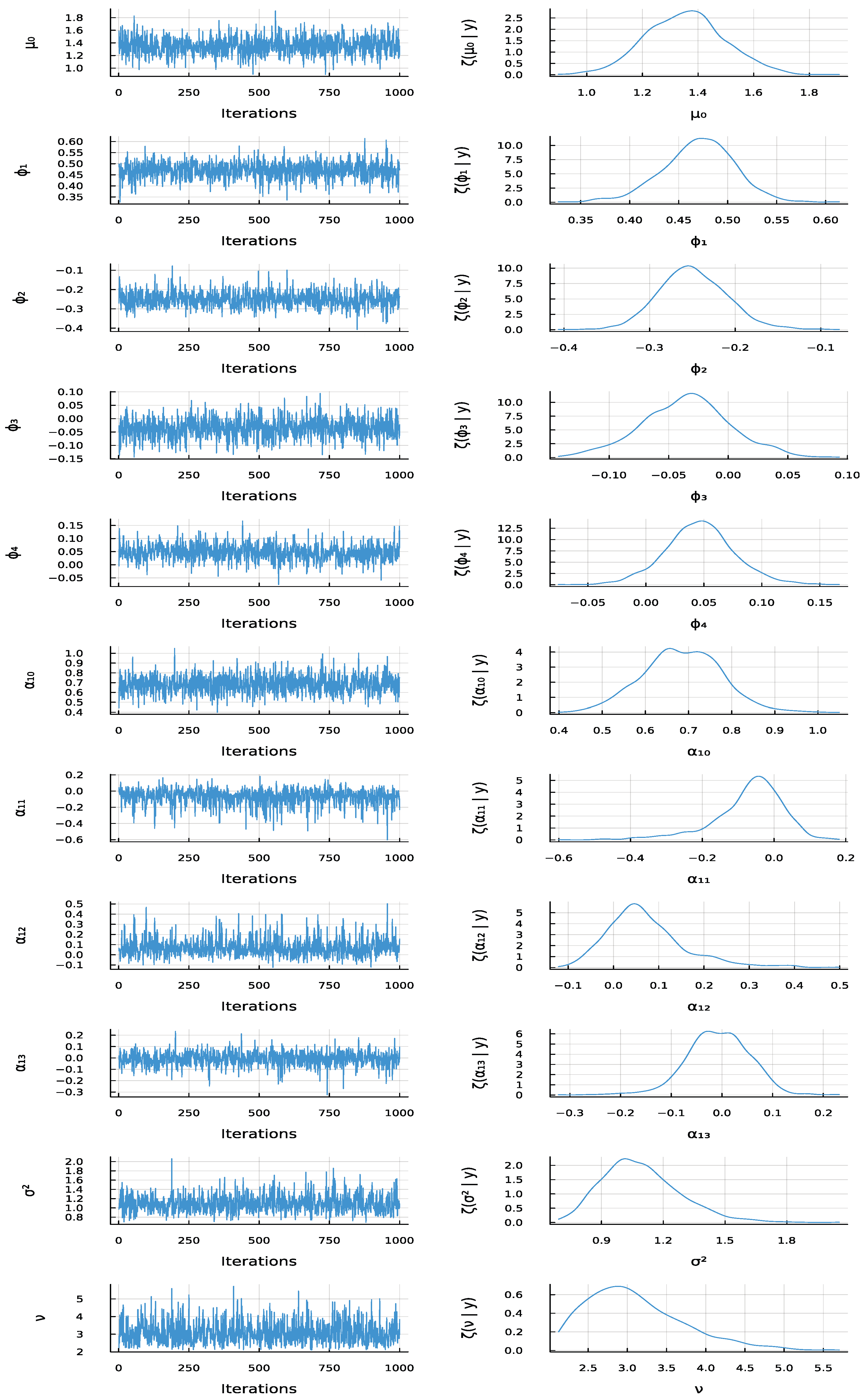
For this representative Model I dataset, MCMC convergence is supported by the diagnostics in

Table 5. Convergence diagnostics of the MCMC chain for one replicate of Model I (SMN-t).

	Raftery–Lewis Diagnostic			Geweke Z-Statistic		Autocorrelations
Parameter	$\mathit{Ntotal}$	$\mathit{Nmin}$	$\mathit{Factor}$	Z-Score	p-Value	Lag 1	Lag 5	Lag 10	Lag 50
${\mu }_0$	893	937	0.953	−0.835	0.404	0.025	−0.018	−0.002	−0.036
${\varphi }_1$	893	937	0.953	0.120	0.904	0.027	−0.010	0.041	0.033
${\varphi }_2$	893	937	0.953	0.933	0.351	−0.007	0.013	0.020	0.014
${\varphi }_3$	1053	937	1.124	−0.193	0.847	0.009	−0.026	0.001	−0.005
${\varphi }_4$	969	937	1.034	0.663	0.507	0.061	−0.050	0.006	−0.028
${\alpha }_{10}$	893	937	0.953	−0.371	0.711	−0.040	0.003	0.009	−0.001
${\alpha }_{11}$	969	937	1.034	−0.519	0.604	0.015	−0.028	0.001	0.048
${\alpha }_{12}$	893	937	0.953	0.081	0.935	0.005	0.052	−0.029	−0.026
${\alpha }_{13}$	969	937	1.034	−1.395	0.163	0.032	−0.047	0.017	0.022
${\sigma }^2$	969	937	1.034	−0.463	0.643	0.110	0.028	−0.061	0.047
$\nu$	893	937	0.953	−1.665	0.096	0.044	0.004	−0.030	−0.014

. Geweke z-scores fall within $(-1.96,1.96)$, the Raftery–Lewis test suggests about 1000 iterations, and empirical autocorrelations of the thinned chain are negligible across all parameters. This conclusion is further reinforced by the trace plots and marginal posterior distributions presented in Figure 1. The trace plots exhibit rapid mixing with no visible trends, drifts, or sustained excursions, consistent with the near-zero autocorrelations of Table 5. The marginal posterior densities are unimodal and approximately symmetric for the AR and exogenous coefficients and moderately right-skewed for the strictly positive scale parameters ${\sigma }^2$ and $\nu$, as expected. No evidence of multimodality or switching between competing lag configurations is apparent in any marginal density, indicating that the sampler concentrates on a single dominant region of the model space corresponding to the true generating structure. Figure 1 thus demonstrates, in a concrete single-dataset setting, the practical reliability of Algorithm 1 before the aggregated results of Section 5.3 are considered.

5.3. Aggregated Results

Identification. We report the rate of exact model identification as both the AR order and the exogenous lag structure simultaneously matching the true generating model. This rate of exact model identification exceeds 80% across all three simulation scenarios and all three SMN distributions. In addition, average marginal posterior inclusion probabilities exceed 0.75 for the active lags, whereas those linked to inactive lags are less than 0.25. This validates the unified SSVS scheme as an effective mechanism for joint AR-order and exogenous-variable selection in the ARX models.

Estimation. 

Table 6. Averaged Bayesian estimation results for Model I. CP: coverage probability of 95% credible intervals.

Parameter	True	$\overline{\mathit{\mu }}$	$\overline{\mathit{\sigma }}$	$\overline{\mathit{L}}$	$\overline{\mathit{U}}$	CP (%)
${\mu }_0$	1.4	1.353	0.163	1.038	1.664	96.0
${\varphi }_1$	0.5	0.492	0.056	0.388	0.597	96.2
${\varphi }_2$	−0.3	−0.290	0.062	−0.402	−0.162	95.6
${\varphi }_3$	0.0	0.000	0.049	−0.091	0.093	99.2
${\varphi }_4$	0.0	0.002	0.043	−0.078	0.083	97.4
${\alpha }_{10}$	0.6	0.595	0.083	0.433	0.753	96.4
${\alpha }_{11}$	0.0	0.001	0.074	−0.129	0.139	99.8
${\alpha }_{12}$	0.0	−0.001	0.071	−0.132	0.129	99.8
${\alpha }_{13}$	0.0	−0.002	0.065	−0.123	0.116	99.6
${\sigma }^2$	1.0	1.053	0.197	0.735	1.505	92.6
$\nu$	3.0	3.212	0.945	2.206	5.768	94.4

,

Table 7. Averaged Bayesian estimation results for Model II.

Parameter	True	$\overline{\mathit{\mu }}$	$\overline{\mathit{\sigma }}$	$\overline{\mathit{L}}$	$\overline{\mathit{U}}$	CP (%)
${\mu }_0$	1.5	1.417	0.174	1.087	1.772	94.6
${\varphi }_1$	0.6	0.610	0.052	0.514	0.712	96.2
${\varphi }_2$	0.0	−0.002	0.049	−0.098	0.090	98.4
${\varphi }_3$	0.0	0.002	0.048	−0.089	0.095	99.6
${\varphi }_4$	0.0	0.004	0.036	−0.068	0.071	98.4
${\alpha }_{10}$	0.7	0.708	0.096	0.517	0.893	92.8
${\alpha }_{11}$	0.4	0.386	0.125	0.099	0.610	93.2
${\alpha }_{12}$	0.0	0.007	0.080	−0.128	0.155	99.4
${\alpha }_{13}$	0.0	−0.005	0.070	−0.137	0.127	99.8
${\alpha }_{20}$	0.6	0.588	0.083	0.425	0.752	95.0
${\alpha }_{21}$	0.0	0.000	0.076	−0.145	0.135	99.2
${\alpha }_{22}$	0.0	0.000	0.069	−0.128	0.121	99.2
${\alpha }_{23}$	0.0	−0.003	0.064	−0.120	0.116	99.8
${\sigma }^2$	1.0	0.953	0.201	0.605	1.407	97.6
$\nu$	0.2	0.247	0.082	0.119	0.447	96.0
$\gamma$	0.1	0.110	0.033	0.058	0.188	94.0

and

Table 8. Averaged Bayesian estimation results for Model III.

Parameter	True	$\overline{\mathit{\mu }}$	$\overline{\mathit{\sigma }}$	$\overline{\mathit{L}}$	$\overline{\mathit{U}}$	CP (%)
${\mu }_0$	1.8	1.665	0.203	1.259	2.051	92.0
${\varphi }_1$	0.7	0.714	0.066	0.590	0.841	94.6
${\varphi }_2$	−0.4	−0.393	0.072	−0.528	−0.253	95.0
${\varphi }_3$	0.0	0.002	0.055	−0.103	0.106	98.6
${\varphi }_4$	0.0	0.011	0.041	−0.067	0.091	98.8
${\alpha }_{10}$	0.5	0.496	0.089	0.321	0.665	96.6
${\alpha }_{11}$	0.0	−0.004	0.077	−0.144	0.134	99.2
${\alpha }_{12}$	0.0	−0.005	0.072	−0.142	0.126	99.8
${\alpha }_{13}$	0.0	−0.007	0.065	−0.130	0.115	99.0
${\alpha }_{20}$	0.6	0.597	0.099	0.410	0.795	92.6
${\alpha }_{21}$	0.4	0.369	0.131	0.064	0.608	93.2
${\alpha }_{22}$	0.0	−0.005	0.081	−0.154	0.136	99.8
${\alpha }_{23}$	0.0	−0.005	0.074	−0.145	0.128	99.0
${\sigma }^2$	1.0	0.988	0.200	0.648	1.437	96.4
$\nu$	2.0	1.991	0.713	1.212	3.905	96.6

report averaged posterior summaries over the 500 replicates for each model under each SMN case. Point estimates are accurate regardless of which SMN member is assumed, and the 95% credible interval averages consistently bracket the true parameter values. Empirical coverage probabilities remain close to the nominal 95% level—typically between 92% and 98%—across parameters and models, apart from those tied to inactive lags. This pattern indicates well-calibrated uncertainty quantification, with interval coverage free from systematic bias.

Forecasting. 

Table 9. RMSE and MWS of simulation results for five-step-ahead Bayesian predictions.

	RMSE				MWS
${\mathit{y}}_{\mathit{n}+\mathit{k}}$	$\mathit{\mu }$	$\mathit{\sigma }$	$\mathit{L}$	$\mathit{U}$	$\mathit{\mu }$	$\mathit{\sigma }$	$\mathit{L}$	$\mathit{U}$
	Model I
$y_{n+1}$	1.37	1.39	0.07	4.63	11.25	30.44	5.16	57.51
$y_{n+2}$	1.68	1.49	0.05	5.34	12.61	29.51	5.92	85.10
$y_{n+3}$	1.62	1.39	0.07	4.37	11.51	25.52	5.92	48.48
$y_{n+4}$	1.61	1.48	0.05	5.43	12.90	25.30	5.99	81.48
$y_{n+5}$	1.86	2.07	0.07	5.82	17.13	55.92	6.05	103.08
	Model II
$y_{n+1}$	1.66	1.46	0.06	5.33	12.43	23.12	5.79	86.26
$y_{n+2}$	2.38	1.85	0.11	6.56	18.57	35.79	6.80	118.91
$y_{n+3}$	2.72	2.21	0.11	7.94	23.69	45.55	7.14	147.63
$y_{n+4}$	2.95	2.25	0.12	7.75	29.08	48.42	6.74	162.62
$y_{n+5}$	3.26	2.46	0.14	8.60	33.86	54.88	7.24	202.76
	Model III
$y_{n+1}$	1.55	1.18	0.08	4.54	10.75	20.29	4.95	64.42
$y_{n+2}$	1.93	1.45	0.06	5.32	12.96	20.81	6.18	74.72
$y_{n+3}$	3.00	2.10	0.16	7.81	32.60	47.95	6.27	177.25
$y_{n+4}$	2.71	2.18	0.13	7.92	29.10	51.14	6.32	187.51
$y_{n+5}$	3.01	2.14	0.17	8.26	32.54	48.88	6.38	190.08

displays the RMSE and MWS values for five-step-ahead Bayesian predictions averaged over the 500 replicates. Across all three ARX configurations and SMN cases, the RMSE stays approximately one standard deviation of the underlying series, and the MWS is comparable to the width of the 95% credible interval. Both RMSE and MWS rise slightly with horizon length, consistent with accumulating disturbance uncertainty. The three SMN cases produce nearly indistinguishable forecasting performance. This indicates that the framework’s predictive accuracy is largely insensitive to the choice of mixing distribution under the baseline design of Table 1, which features moderate degrees of freedom, a moderate contamination level, and a sample size of $n=200$. Robustness under more severe contamination or alternative sample sizes is examined only to the extent reported below, and remains an important avenue for further investigation.

Across the 500 replicates, the average Metropolis–Hastings acceptance rates are about 92% and 68% for the SMN-t and the SMN-cn cases, respectively. These values fall comfortably within standard ranges, indicating that the samplers explore their respective posterior distributions efficiently. Moreover, across all simulation scenarios, the MCMC chains satisfy the convergence diagnostics, confirming that the reported posterior and predictive summaries are derived from properly converged simulations. Under the simulation settings used, each complete run of the MCMC algorithm takes on average less than 14 seconds per dataset on a standard laptop (Intel Core i7, 16 GB RAM, Julia 1.12.6).

Effect of sample size. To assess how estimation and forecasting accuracy scale with the length of the observed series, we re-estimate Model I (SMN-t) at sample sizes $n=100$ and $n=300$, keeping every other design element unchanged from Table 1.

Table 10. Averaged Bayesian estimation results for Model I (SMN-t) with sample sizes $n=100$ and $n=300$.

Parameter	$\mathit{True}$	$\overline{\mathit{\mu }}$	$\overline{\mathit{\sigma }}$	$\overline{\mathit{L}}$	$\overline{\mathit{U}}$	CP (%)	$\overline{\mathit{\mu }}$	$\overline{\mathit{\sigma }}$	$\overline{\mathit{L}}$	$\overline{\mathit{U}}$	CP (%)
		$\mathit{n}=\mathbf{100}$					$\mathit{n}=\mathbf{300}$
${\mu }_0$	1.4	1.279	0.236	0.825	1.731	96.4	1.367	0.131	1.115	1.616	96.2
${\varphi }_1$	0.5	0.488	0.084	0.329	0.642	95.6	0.504	0.043	0.421	0.586	94.0
${\varphi }_2$	−0.3	−0.276	0.095	−0.445	−0.059	92.8	−0.296	0.048	−0.387	−0.204	96.2
${\varphi }_3$	0.0	−0.003	0.064	−0.121	0.114	99.6	0.000	0.041	−0.078	0.077	97.0
${\varphi }_4$	0.0	0.011	0.056	−0.092	0.115	98.6	0.005	0.035	−0.063	0.073	97.4
${\alpha }_{10}$	0.6	0.575	0.125	0.340	0.805	96.4	0.593	0.067	0.467	0.723	97.4
${\alpha }_{11}$	0.0	0.006	0.103	−0.166	0.206	99.6	0.004	0.063	−0.112	0.124	99.7
${\alpha }_{12}$	0.0	−0.007	0.099	−0.197	0.157	99.6	0.001	0.060	−0.112	0.114	99.4
${\alpha }_{13}$	0.0	−0.003	0.087	−0.161	0.151	99.7	−0.001	0.055	−0.107	0.103	98.8
${\sigma }^2$	1.0	1.064	0.291	0.642	1.777	95.0	1.000	0.153	0.746	1.344	96.4
$\nu$	3.0	3.239	1.738	2.162	8.011	97.0	2.983	0.600	2.202	4.524	95.6

reports averaged posterior summaries over the 500 replicates for Model I (SMN-t) with sample sizes $n=100$ and $n=300$, while

Table 11. RMSE and MWS of simulation results for five-step-ahead Bayesian predictions of Model I (SMN-t) with sample sizes $n=100$ and $n=300$.

	RMSE				MWS
${\mathit{y}}_{\mathit{n}+\mathit{k}}$	$\mathit{\mu }$	$\mathit{\sigma }$	$\mathit{L}$	$\mathit{U}$	$\mathit{\mu }$	$\mathit{\sigma }$	$\mathit{L}$	$\mathit{U}$
	$n=100$
$y_{n+1}$	1.45	1.28	0.05	4.10	10.31	23.40	4.97	39.29
$y_{n+2}$	1.91	1.51	0.05	5.14	13.23	27.78	5.76	60.95
$y_{n+3}$	2.36	1.62	0.13	6.42	17.60	27.51	5.76	103.03
$y_{n+4}$	2.02	1.57	0.07	5.82	14.35	26.15	5.78	81.63
$y_{n+5}$	1.92	1.54	0.07	5.62	14.51	26.95	5.81	88.63
	$n=300$
$y_{n+1}$	1.25	1.10	0.03	3.97	9.15	17.55	5.29	47.37
$y_{n+2}$	1.60	1.48	0.07	5.33	12.72	27.95	6.05	71.14
$y_{n+3}$	1.64	1.53	0.06	5.73	13.41	31.20	6.16	88.07
$y_{n+4}$	1.57	1.38	0.06	5.46	12.02	22.37	6.15	94.95
$y_{n+5}$	1.61	1.35	0.10	5.04	11.49	19.61	6.17	61.00

displays the RMSE and MWS values for five-step-ahead Bayesian predictions averaged over the 500 replicates. These two tables are read alongside the $n=200$ baseline already reported in Table 6 and Table 9.

Posterior uncertainty contracts systematically as n grows. Averaged across the AR and exogenous coefficients, posterior standard deviations fall by roughly half between $n=100$ and $n=300$ (e.g., ${\overline{\sigma }}_{{\mu }_0}$: 0.236 → 0.131; ${\overline{\sigma }}_{{\varphi }_1}$: 0.084 → 0.043), consistent with the usual posterior contraction rate for regular parametric models. The degrees-of-freedom parameter $\nu$ is by far the most sample-size-sensitive quantity. Its posterior standard deviation shrinks from 1.738 at $n=100$ to 0.945 at $n=200$ (Table 6) to 0.600 at $n=300$, reflecting the well-documented difficulty of pinning down the tail heaviness of a Student-t distribution from short series. Posterior bias is likewise reduced at larger n—for example, ${\overline{\mu }}_{{\varphi }_1}$ moves from 0.488 ($n=100$) to 0.492 ($n=200$) to 0.504 ($n=300$), converging toward the true value 0.5. Coverage probabilities for the active coefficients stay close to the nominal 95% level at every sample size (92.8–97.4%), while coefficients tied to inactive lags continue to show the mild overcoverage already noted for $n=200$ (97.0–99.8%), indicating that the SSVS shrinkage mechanism does not compromise interval calibration even when the series is comparatively short.

These patterns carry over to forecasting. RMSE in Table 11 decreases essentially monotonically in n at every horizon (e.g., $y_{n+1}$: 1.45 at $n=100$ versus 1.25 at $n=300$; $y_{n+5}$: 1.92 versus 1.61), confirming that sharper parameter estimates at larger n translate directly into more accurate point forecasts. MWS exhibits the same broad pattern of improvement but with greater horizon-to-horizon variability. For example, at $h=1$ the $n=100$ case attains a lower average MWS than the $n=200$ baseline (10.31 versus 11.25), despite its larger RMSE. This behavior is consistent with the substantially heavier right skew of the MWS distribution relative to RMSE across replicates. Because the Winkler score penalizes interval misses heavily, its 500-replicate average is more sensitive than RMSE to a handful of runs with wide or missed intervals. The underlying improvement with n is nonetheless clearly visible by $n=300$, where MWS is lower than the $n=200$ baseline at every horizon.

Effect of contamination level. To assess robustness to a higher proportion of outlying observations, we re-estimate Model II (SMN-cn) with contamination probabilities $\nu =0.3$ and $\nu =0.4$, holding every other design element unchanged from Table 1.

Table 12. Averaged Bayesian estimation results for Model II (SMN-cn) with contamination probabilities $\nu =0.3$ and $\nu =0.4$.

Parameter	$\mathit{True}$	$\overline{\mathit{\mu }}$	$\overline{\mathit{\sigma }}$	$\overline{\mathit{L}}$	$\overline{\mathit{U}}$	CP (%)	$\overline{\mathit{\mu }}$	$\overline{\mathit{\sigma }}$	$\overline{\mathit{L}}$	$\overline{\mathit{U}}$	CP (%)
		$\nu =\mathbf{0}.\mathbf{3}$					$\nu =\mathbf{0}.\mathbf{4}$
${\mu }_0$	1.5	1.400	0.180	1.046	1.753	92.0	1.380	0.194	1.002	1.758	92.8
${\varphi }_1$	0.6	0.611	0.051	0.514	0.711	96.6	0.611	0.052	0.514	0.712	94.6
${\varphi }_2$	0.0	−0.002	0.048	−0.095	0.089	96.8	−0.002	0.049	−0.094	0.089	98.2
${\varphi }_3$	0.0	0.003	0.047	−0.086	0.094	99.4	0.000	0.048	−0.089	0.094	99.0
${\varphi }_4$	0.0	0.003	0.037	−0.069	0.072	98.6	0.005	0.038	−0.070	0.076	98.2
${\alpha }_{10}$	0.7	0.707	0.105	0.507	0.922	92.6	0.711	0.120	0.487	0.952	93.4
${\alpha }_{11}$	0.4	0.370	0.141	0.041	0.627	93.0	0.355	0.157	0.012	0.647	91.2
${\alpha }_{12}$	0.0	0.005	0.086	−0.141	0.158	99.4	0.007	0.094	−0.149	0.180	99.8
${\alpha }_{13}$	0.0	−0.004	0.076	−0.150	0.133	99.2	−0.003	0.082	−0.157	0.145	99.6
${\alpha }_{20}$	0.6	0.587	0.095	0.405	0.776	95.8	0.584	0.108	0.373	0.792	95.6
${\alpha }_{21}$	0.0	−0.003	0.083	−0.158	0.140	99.4	−0.003	0.091	−0.170	0.155	99.4
${\alpha }_{22}$	0.0	0.001	0.074	−0.136	0.133	99.4	0.001	0.081	−0.148	0.144	99.4
${\alpha }_{23}$	0.0	−0.002	0.067	−0.125	0.120	99.8	−0.002	0.073	−0.134	0.127	99.8
${\sigma }^2$	1.0	1.001	0.247	0.567	1.565	97.4	1.060	0.316	0.536	1.826	97.2
$\nu$	$\nu$	0.332	0.086	0.179	0.523	97.2	0.408	0.094	0.229	0.605	98.6
$\gamma$	0.1	0.104	0.032	0.056	0.180	97.8	0.103	0.033	0.056	0.186	97.6

reports averaged posterior summaries over the 500 replicates for Model II (SMN-cn) with contamination probabilities $\nu =0.3$ and $\nu =0.4$, and

Table 13. RMSE and MWS of simulation results for five-step-ahead Bayesian predictions of Model II (SMN-cn) with contamination probabilities $\nu =0.3$ and $\nu =0.4$.

	RMSE				MWS
${\mathit{y}}_{\mathit{n}+\mathit{k}}$	$\mathit{\mu }$	$\mathit{\sigma }$	$\mathit{L}$	$\mathit{U}$	$\mathit{\mu }$	$\mathit{\sigma }$	$\mathit{L}$	$\mathit{U}$
	$\nu =0.3$
$y_{n+1}$	1.80	1.60	0.08	6.10	13.20	21.53	7.45	81.03
$y_{n+2}$	2.54	2.01	0.13	7.59	18.10	34.52	8.10	120.00
$y_{n+3}$	2.85	2.34	0.13	8.36	22.38	44.90	8.57	142.53
$y_{n+4}$	3.02	2.35	0.12	8.47	22.52	37.63	9.11	136.18
$y_{n+5}$	3.36	2.53	0.14	9.28	28.84	50.08	8.21	190.44
	$\nu =0.4$
$y_{n+1}$	1.92	1.69	0.06	6.52	13.61	19.33	8.54	62.77
$y_{n+2}$	2.67	2.13	0.14	8.18	18.44	32.23	9.27	113.02
$y_{n+3}$	2.95	2.47	0.09	8.89	22.18	46.37	9.76	142.24
$y_{n+4}$	3.16	2.56	0.10	9.41	23.21	41.90	10.15	159.53
$y_{n+5}$	3.44	2.67	0.18	9.88	27.68	49.42	9.45	192.85

displays the RMSE and MWS values for five-step-ahead Bayesian predictions averaged over the 500 replicates; both are read alongside the $\nu =0.2$ baseline already reported in Table 7 and Table 9.

Increasing the contamination probability from $\nu =0.2$ to $\nu =0.4$—so that up to 40% of observations are drawn from the high-variance contaminating component—leaves posterior means close to their true values throughout, with no evidence of systematic bias emerging as contamination becomes more frequent. ${\overline{\mu }}_{{\varphi }_1}$ remains at 0.610–0.611 across all three contamination levels, and the inactive coefficients continue to be shrunk toward zero (e.g., ${\overline{\mu }}_{{\alpha }_{12}}$ stays within 0.007 of its true value at every $\nu$). Posterior uncertainty widens as the sample becomes noisier, as expected. The posterior standard deviation grows with $\nu$ for both the AR and exogenous coefficients (e.g., ${\overline{\sigma }}_{{\mu }_0}$: 0.174, 0.180, 0.194; ${\overline{\sigma }}_{{\alpha }_{11}}$: 0.125, 0.141, 0.157, at $\nu =0.2,0.3,0.4$) and the error scale (${\overline{\sigma }}_{{\sigma }^2}$: 0.201, 0.247, 0.316). Coverage probabilities for the active coefficients remain broadly acceptable at $\nu =0.3$ and $\nu =0.4$ (91.2–96.6%), while inactive-lag and scale/shape parameters continue to show good-to-mild overcoverage (96.8–99.8%). The contamination parameters themselves remain well identified at every setting. The posterior mean of $\nu$ tracks its true value closely (0.247, 0.332, and 0.408 against true values 0.2, 0.3, and 0.4), and $\gamma$ is recovered accurately throughout (${\overline{\mu }}_{\gamma }\approx 0.10$–$0.11$ against a true value of 0.1).

Forecast accuracy degrades in the expected direction as contamination intensifies. RMSE in Table 13 increases monotonically with $\nu$ at every horizon relative to the $\nu =0.2$ baseline in Table 9 (e.g., $y_{n+1}$: 1.66, 1.80, 1.92; $y_{n+5}$: 3.26, 3.36, 3.44), confirming that a larger proportion of outlying observations makes point forecasts modestly less precise, as anticipated. MWS, by contrast, does not increase as cleanly with $\nu$. As in the sample-size comparison above, this is consistent with the very heavy right skew of the Winkler score across replicates. The RMSE pattern is unambiguous and is the more reliable indicator of the (modest and expected) forecasting cost of heavier contamination.We emphasize that this robustness evidence is confined to contamination probabilities up to $\nu =0.4$ under the SMN-cn mixing distribution with $\gamma =0.1$ fixed. Substantially more severe contamination levels, alternative contamination scales, and deliberate model misspecification (e.g., fitting the ARX-SMN model to data generated from a non-SMN error process) were not examined. The robustness claims of this paper should therefore be read as applying specifically to the SMN error families and contamination levels investigated in this section, rather than as a general guarantee of robustness under arbitrary departures from the assumed model.

6. Empirical Application: Daily Solar Radiation in Najran, Saudi Arabia

6.1. Background and Data Description

Accurate forecasting of solar irradiance is a critical enabler of reliable planning and dispatch in solar energy systems [6,7]. Saudi Arabia possesses some of the world’s highest solar energy potential, with annual global horizontal irradiance (GHI) routinely exceeding $2000\mathrm{kWh}/{\mathrm{m}}^2$ [46,47]. The southern region of Najran is particularly noteworthy: situated at approximately $17.5°$ N latitude, it benefits from persistently high direct-normal irradiance values and a strategic geographic position for the country’s Vision 2030 renewable energy targets [46]. This resource richness motivates the present application of a probabilistic forecasting model to Najran solar radiation.

We analyze a continuous 80-day record of daily meteorological observations from the Najran ground station, spanning from 1 December 2005 to 18 February 2006 ($n_{\mathrm{raw}}=80$). This winter sub-sample captures a period of changing solar angles and variable cloud-cover conditions without the strongly deterministic extremes of the Saudi summer, providing a challenging but realistic forecasting environment.

Two time series are employed:

• Global Horizontal Irradiance (GHI) [$y_t$, endogenous]: the total daily shortwave radiation received on a horizontal surface at ground level, encompassing both direct beam and diffuse components, measured in Wh/m² by a pyranometer at the Najran meteorological station. GHI is the primary target variable in solar energy forecasting because it determines the potential electricity yield of a photovoltaic installation [6,48].
• Clear-Sky GHI [$x_t$, exogenous]: the theoretical GHI that would be recorded on a completely cloudless day, computed from a radiative-transfer model using solar geometry (latitude, Earth–Sun distance, hour angle), and a standard atmospheric composition (aerosol optical depth, water vapor, ozone) [48,49]. Because clear-sky GHI captures the deterministic astronomical variation in available solar energy, it serves as an ideal external driver for the ARX model. It tracks the slowly changing baseline around which the actual GHI fluctuates due to transient meteorological factors.

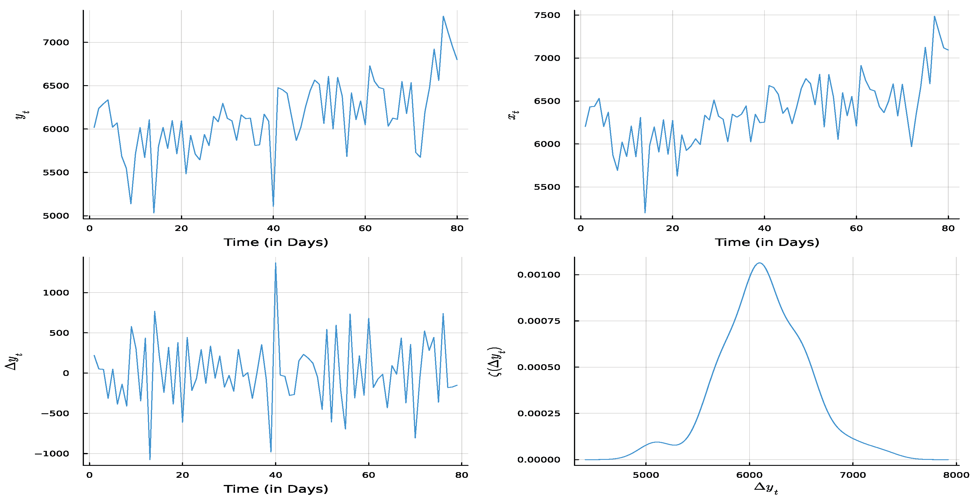
The two daily GHI and Clear-Sky GHI series are shown in Figure 2, and their descriptive statistics are summarized in

Table 14. Descriptive statistics for raw daily Najran solar radiation, 1 December 2005—18 February 2006 ($n_{\mathrm{raw}}=80$). CV: coefficient of variation.

Variable	Mean	Std. Dev.	Min	Max	CV (%)
GHI (Wh/m2)	6135.2	414.9	5033.0	7302.0	6.76
Clear-Sky GHI (Wh/m2)	6369.5	376.7	5198.0	7487.0	5.91

. From Table 14, the observed mean daily GHI ($6135.2\mathrm{Wh}/{\mathrm{m}}^2$) falls considerably below the clear-sky mean ($6369.5\mathrm{Wh}/{\mathrm{m}}^2$), quantifying the average atmospheric attenuation from clouds, aerosols, and humidity. Strikingly, the coefficient of variation of GHI (6.76%) is more than that of clear-sky GHI (5.91%), reflecting the dominant role of transient weather variability in driving actual radiation fluctuations, whereas clear-sky GHI evolves slowly according to astronomical cycles alone.

6.2. Stationarity Transformations

Direct modeling of the GHI and clear-sky GHI in their raw levels is inadvisable for two reasons. First, both series exhibit a local deterministic trend caused by the steadily changing day length between December and mid-February, inducing non-stationarity and potentially spurious correlations [7,50]. Second, the difference in magnitudes between the two variables can produce numerical instability in the MCMC sampler. We therefore apply a two-step preprocessing pipeline. In the first step, each series is standardized to zero mean and unit variance using its sample mean and standard deviation, yielding $y_t^{\ast }=(y_t-\overline{y})/s_y$ and $x_t^{\ast }=(x_t-\overline{x})/s_x$. In the second step, first differences are applied: $\Delta y_t=y_t^{\ast }-y_{t-1}^{\ast }$ and $\Delta x_t=x_t^{\ast }-x_{t-1}^{\ast }$. The resulting series $\{\Delta y_t\}$ and $\{\Delta x_t\}$ represent standardized day-to-day changes in observed and clear-sky GHI, respectively. By filtering out the slow astronomical trend, differencing isolates the short-term meteorological dynamics—such as the effect of a cloud event on the following day’s radiation budget—that are the primary target of the ARX model. The density of $\{\Delta y_t\}$ in Figure 2 exhibits moderate excess kurtosis and occasional outliers corresponding to abrupt weather transitions (e.g., sudden dust storms or heavy cloud intrusions), providing empirical justification for the SMN error assumption [29,51].

The transformed dataset has $n=79$ usable observations after differencing. We partition this into a training set of $n_{\mathrm{tr}}=69$ observations and a hold-out test set of $n_{\mathrm{te}}=10$ observations to evaluate out-of-sample forecast accuracy.

6.3. Bayesian ARX Analysis of Daily Najran Solar Radiation

Algorithm 1 is applied to the training set of the transformed series $\{\Delta y_t\}$ with exogenous input $\{\Delta x_t\}$, using $p_{max}=5$, $d_{1,max}=5$, and $k=10$ for the forecast horizon. The MCMC settings are $N_{\mathrm{sim}}=\mathrm{11,000}$, $N_{\mathrm{burn}}=1000$, and $N_{\mathrm{thin}}=10$. Future clear-sky GHI values over the 10-day test window are taken from the observed clear-sky record, which is known in advance from astronomical calculations and represents no forecasting challenge [48,49].

Model identification. 

Table 15. Posterior inclusion probabilities of latent-indicators for the Najran daily GHI change series under SMN distributions.

	${\mathit{\delta }}^{\mathit{\varphi }}$					${\mathit{\delta }}^{\mathit{\alpha }}$
SMN	${\delta }_{\mathbf{1}}^{\varphi }$	${\delta }_{\mathbf{2}}^{\varphi }$	${\delta }_{\mathbf{3}}^{\varphi }$	${\delta }_{\mathbf{4}}^{\varphi }$	${\delta }_{\mathbf{5}}^{\varphi }$	${\delta }_{\mathbf{10}}^{\alpha }$	${\delta }_{\mathbf{11}}^{\alpha }$	${\delta }_{\mathbf{12}}^{\alpha }$	${\delta }_{\mathbf{13}}^{\alpha }$	${\delta }_{\mathbf{14}}^{\alpha }$
SMN-t	0.740	0.581	0.448	0.326	0.110	0.999	0.675	0.524	0.410	0.199
SMN-sl	0.859	0.714	0.474	0.351	0.077	0.999	0.813	0.654	0.470	0.221
SMN-cn	0.168	0.107	0.131	0.081	0.099	0.999	0.125	0.121	0.106	0.103
SMN-n	0.967	0.634	0.398	0.154	0.091	0.999	0.961	0.672	0.422	0.140

presents the posterior inclusion probabilities of latent indicators of the ARX model from the 1000 retained MCMC draws, reported for each of the four SMN distributions. The latent indicators ${\mathit{\delta }}^{\varphi }=({\delta }_1^{\varphi },\dots ,{\delta }_5^{\varphi })$ govern AR lag inclusion, and ${\mathit{\delta }}^{\alpha }=({\delta }_{10}^{\alpha },\dots ,{\delta }_{14}^{\alpha })$ governs clear-sky GHI lag inclusion. Across all four SMN specifications, except of the SMN-cn case, the latent indicators with the highest posterior inclusion probability corresponds to the ARX(2,3) model, comprising the first two AR lags and the first three lags of the clear-sky GHI change. This structure admits a natural physical interpretation. The two AR lags reflect a two-day cloud memory. The three clear-sky lags (${\alpha }_{10},{\alpha }_{11},{\alpha }_{12}$) reflect the multi-day influence of atmospheric conditions. The contemporaneous lag ${\alpha }_{10}$ accounts for the direct modulation of actual GHI by the prevailing clear-sky envelope. The two successive lagged coefficients capture the gradual dissipation of aerosol loading and humidity anomalies that attenuate radiation over consecutive days before the atmosphere returns to its baseline state. The relative disagreement of the SMN-cn specification underscores the sensitivity of variable selection to the assumed tail behavior under the contaminated normal, where the heavier contamination component may absorb part of the signal otherwise attributed to the higher-order lags.

Parameter estimates. Beyond the model-identification results above,

Table 16. Bayesian estimates for the Najran daily GHI change series under SMN distributions.

Parameter	$\mathit{\mu }$	$\mathit{\sigma }$	L	U	$\mathit{\mu }$	$\mathit{\sigma }$	L	U
	SMN-$\mathit{t}$				SMN-sl
${\mu }_0$	0.0643	0.0345	−0.0038	0.1278	0.0696	0.0347	−0.0071	0.1315
${\varphi }_1$	−0.6072	0.3000	−1.0081	−0.0959	−0.7770	0.2696	−1.0129	−0.1253
${\varphi }_2$	−0.3211	0.2763	−0.9043	−0.0360	−0.5412	0.2619	−0.8914	−0.0391
${\varphi }_3$	−0.2244	0.2171	−0.7191	−0.0152	−0.3571	0.2116	−0.7494	−0.0200
${\varphi }_4$	−0.1567	0.1523	−0.5091	0.0136	−0.2309	0.1453	−0.5018	0.0084
${\varphi }_5$	−0.0137	0.0517	−0.1068	0.0890	−0.0287	0.0546	−0.1182	0.0873
${\alpha }_{10}$	0.8861	0.0477	0.7980	0.9832	0.9066	0.0490	0.8106	0.9932
${\alpha }_{11}$	0.5329	0.2972	0.0423	0.9643	0.7134	0.2718	0.0831	0.9957
${\alpha }_{12}$	0.2575	0.2840	−0.0353	0.8649	0.4881	0.2778	−0.0177	0.8844
${\alpha }_{13}$	0.1749	0.2174	−0.0440	0.6819	0.2644	0.2252	−0.0569	0.7084
${\alpha }_{14}$	0.0793	0.1339	−0.0813	0.4160	0.1163	0.1329	−0.0863	0.3964
${\sigma }^2$	0.0279	0.0122	0.0129	0.0596	0.0201	0.0089	0.0097	0.0440
$\nu$	2.2787	0.2789	2.1058	3.1338	1.0801	0.1483	1.0022	1.5015
	SMN-cn				SMN-n (Gaussian)
${\mu }_0$	0.0213	0.0183	−0.0138	0.0592	0.0046	0.0546	−0.1058	0.1103
${\varphi }_1$	−0.1184	0.1012	−0.3631	0.0035	−0.7390	0.1949	−1.0981	−0.3445
${\varphi }_2$	−0.0841	0.0819	−0.2101	0.0280	−0.4183	0.2679	−0.9689	−0.0390
${\varphi }_3$	−0.0826	0.0664	−0.1770	0.0143	−0.2058	0.2258	−0.7723	0.0418
${\varphi }_4$	−0.0396	0.0508	−0.1202	0.0376	−0.0579	0.1284	−0.3466	0.1515
${\varphi }_5$	0.0022	0.0196	−0.0360	0.0408	0.0267	0.0714	−0.1167	0.1643
${\alpha }_{10}$	0.8515	0.0200	0.8106	0.8861	0.9426	0.0930	0.7426	1.1191
${\alpha }_{11}$	0.0866	0.0917	−0.0219	0.2846	0.8002	0.2359	0.2713	1.2143
${\alpha }_{12}$	0.0721	0.0772	−0.0374	0.1920	0.4656	0.3255	−0.0122	1.1329
${\alpha }_{13}$	0.0638	0.0663	−0.0429	0.1616	0.2016	0.2707	−0.1041	0.8611
${\alpha }_{14}$	0.0292	0.0454	−0.0483	0.1037	0.0362	0.1339	−0.1748	0.3436
${\sigma }^2$	0.0050	0.0027	0.0025	0.0112	0.2276	0.0537	0.1514	0.3624
$\nu$	0.3580	0.0725	0.2293	0.5089	–	–	–	–
$\gamma$	0.0059	0.0037	0.0026	0.0160	–	–	–	–

additionally reports the full Bayesian posterior summaries of every model parameter estimated directly on the real Najran GHI series, providing an empirical evaluation of the proposed methodology under authentic, non-simulated conditions that complements the controlled simulation results of Section 5. Table 16 reports the Bayesian posterior summaries of all model parameters under each of the four SMN distributions. The intercept ${\mu }_0$ carries a posterior mean close to zero and a 95% credible interval that includes zero in all four cases, consistent with the near-zero unconditional mean of the differenced standardized series. Turning to the AR structure, a striking and physically meaningful pattern emerges: the posterior means of all active AR coefficients are negative across every SMN specification. Under SMN-t, the first three AR lags have 95% credible intervals that exclude zero, i.e., the posterior evidence supports a non-zero effect, with posterior means ${\varphi }_1\approx -0.607$, ${\varphi }_2\approx -0.321$, and ${\varphi }_3\approx -0.224$, while ${\varphi }_4$ and ${\varphi }_5$ have credible intervals that include zero. A qualitatively similar pattern is observed under the other SMN cases. Under SMN-cn, the AR coefficients are substantially attenuated, and only ${\varphi }_1$’s credible interval lies just outside zero ($\approx -0.118$), reflecting the fact that the contaminated normal absorbs a larger share of the observed variability through its mixing component. The consistent negativity of the AR coefficients in the differenced series is physically interpretable as mean-reverting oscillatory dynamics in daily GHI changes. An anomalously large positive change on a given day—associated, for instance, with a sudden clearing of cloud cover—tends to be followed by a partial downward correction over subsequent days, as the atmosphere gradually returns to its ambient aerosol and humidity equilibrium.

Among the exogenous clear-sky coefficients, ${\alpha }_{10}$ is by far the dominant driver. Its 95% credible interval excludes zero by a wide margin in all four cases, providing strong posterior evidence for a non-zero effect. This confirms that the contemporaneous change in clear-sky GHI is the single most informative predictor of observed GHI changes. The first lagged coefficient ${\alpha }_{11}$ also has a credible interval that excludes zero under SMN-t (≈0.533), SMN-sl (≈0.713), and SMN-n (≈0.800), capturing the residual influence of the previous day’s atmospheric state on current radiation levels. The higher lags ${\alpha }_{12}$, ${\alpha }_{13}$, and ${\alpha }_{14}$ carry credible intervals that include zero across all specifications, indicating that their contributions are negligible once the contemporaneous and first-lagged clear-sky signals are accounted for. These lags illustrate concretely the joint reading of posterior inclusion probabilities (PIP) and credible intervals set out in Section 4.2. Under SMN-t, ${\alpha }_{12}$ has an intermediate PIP of 0.524 (Table 15) together with a 95% credible interval of $(-0.035,0.865)$ that includes zero (Table 16). Both quantities agree on the same substantive conclusion, i.e., roughly half of the retained draws support, including this lag, and the BMA-averaged effect, while positive on average, is not sharply distinguishable from zero. So, the two summaries reinforce rather than contradict one another once it is recognized that the reported credible interval already averages over both the included and excluded mixture components.

The SMN-specific parameter estimates provide particularly informative evidence about the distributional character of the radiation residuals. Under SMN-t, the estimated degrees of freedom $\widehat{\nu }\approx 2.28$, which signals extremely heavy-tailed innovations, consistent with abrupt meteorological discontinuities such as dust intrusions and sudden cloud-cover transitions. The SMN-sl estimate $\widehat{\nu }\approx 1.08$ similarly places the error distribution near the Cauchy family, corroborating the presence of large occasional deviations. Under SMN-cn, the estimated contamination probability $\widehat{\nu }\approx 0.358$ indicates that approximately 36% of daily observations arise from a contaminating component. The estimated contamination scale $\widehat{\gamma }\approx 0.006$ implies that this component carries a variance of ${\widehat{\sigma }}^2/\widehat{\gamma }\approx 0.83$, roughly 167 times larger than the dominant component variance ${\widehat{\sigma }}^2\approx 0.005$, capturing the high-amplitude outliers produced by episodic extreme weather events. The scale parameter ${\sigma }^2$ itself varies markedly across distributions—from $0.005$ under SMN-cn to $0.228$ under SMN-n. This is because the heavy-tailed specifications attribute large residuals to the mixing component rather than to ${\sigma }^2$, leaving a much tighter residual core. The inflated ${\sigma }^2$ estimate under SMN-n thus reflects the inadequacy of the Gaussian assumption for this dataset. Despite these distributional differences, all four SMN cases produce broadly concordant estimates of the dynamic and exogenous coefficients, demonstrating that structural inference on the ARX model is robust to the precise choice of tail specification. Across all four SMN cases, MCMC chains pass the Geweke and Raftery–Lewis diagnostics, confirming the convergence of the chains. The Metropolis–Hastings acceptance rates are about 95% and 70% for the SMN-t and the SMN-cn cases, respectively.

Forecasting. 

Table 17. Ten-step-ahead Bayesian forecasts of differenced-standardized daily GHI at Najran under four SMN distributions. $\mu$: posterior forecast mean; $\sigma$: posterior forecast SD; L, U: 95% credible bounds.

${\mathit{y}}_{\mathit{n}+\mathit{k}}$	${\mathit{y}}_{\mathit{n}+1}$	${\mathit{y}}_{\mathit{n}+2}$	${\mathit{y}}_{\mathit{n}+3}$	${\mathit{y}}_{\mathit{n}+4}$	${\mathit{y}}_{\mathit{n}+5}$	${\mathit{y}}_{\mathit{n}+6}$	${\mathit{y}}_{\mathit{n}+7}$	${\mathit{y}}_{\mathit{n}+8}$	${\mathit{y}}_{\mathit{n}+9}$	${\mathit{y}}_{\mathit{n}+10}$
True	−1.94	−0.13	1.26	0.68	1.07	−0.87	1.79	−0.43	−0.41	−0.36
	SMN-t
$\mu$	−0.947	−0.892	1.132	0.560	1.314	−0.943	1.599	−0.433	−0.500	0.217
$\sigma$	0.393	0.484	0.549	0.499	0.485	0.401	0.467	0.430	0.495	0.591
L	−1.560	−1.736	0.238	−0.353	0.387	−1.751	0.586	−1.211	−1.365	−0.561
U	−0.158	−0.042	2.123	1.502	2.259	−0.135	2.439	0.424	0.282	1.492
RMSE	0.995	0.759	0.128	0.117	0.244	0.071	0.187	0.001	0.086	0.579
	SMN-sl
$\mu$	−0.982	−0.939	1.249	0.535	1.444	−1.003	1.518	−0.408	−0.532	0.326
$\sigma$	0.325	0.425	0.509	0.491	0.455	0.398	0.621	0.444	0.417	0.533
L	−1.594	−1.739	0.405	−0.401	0.564	−1.831	0.569	−1.242	−1.372	−0.544
U	−0.346	−0.080	2.191	1.460	2.338	−0.261	2.432	0.426	0.283	1.532
RMSE	0.961	0.806	0.011	0.143	0.374	0.131	0.268	0.026	0.118	0.688
	SMN-cn
$\mu$	−0.851	−0.828	0.909	0.700	1.077	−0.945	1.764	−0.473	−0.398	−0.002
$\sigma$	0.555	0.588	0.582	0.556	0.577	0.568	0.563	0.570	0.598	0.592
L	−2.093	−2.259	−0.391	−0.675	−0.397	−2.381	0.385	−2.002	−1.860	−1.536
U	0.542	0.502	2.361	2.061	2.373	0.386	3.017	0.686	1.065	1.371
RMSE	1.092	0.695	0.351	0.023	0.007	0.073	0.022	0.039	0.017	0.360
	SMN-n (Gaussian)
$\mu$	−0.960	−0.970	0.968	0.726	1.389	−0.968	1.686	−0.214	−0.499	0.091
$\sigma$	0.529	0.659	0.674	0.700	0.696	0.668	0.723	0.688	0.703	0.759
L	−2.073	−2.269	−0.285	−0.659	0.076	−2.335	0.166	−1.557	−2.010	−1.281
U	0.050	0.273	2.447	2.019	2.754	0.316	3.146	1.092	0.755	1.705
RMSE	0.983	0.837	0.293	0.049	0.319	0.095	0.100	0.220	0.085	0.453

presents the 10-step-ahead Bayesian forecasts of the standardized-differenced GHI series for the held-out test period, together with the true observed values and forecast accuracy metrics. Under all four SMN distributions, most of the 10 true values fall within the 95% credible intervals, validating the calibration of the predictive distribution. The RMSE values are small in every case—below 1.1 standardized units at all horizons—consistent with the general finding that clear-sky GHI provides an informative structural signal that reduces residual uncertainty. We compute the RMSE of the 10-step-ahead Bayesian forecasts for the anti-transformed daily GHI series; for the ARX model, the RMSEs are approximately 153.9 (SMN-t), 161.1 (SMN-sl), 159.0 (SMN-cn), and 163.1 (SMN-n), all of which are small relative to the daily GHI series’ standard deviation. Accordingly, based on point RMSE, the ARX specification with SMN-t attains the lowest anti-transformed forecast error among the four fitted SMN cases for this series. With only ten held-out horizons, however, this ranking should be interpreted as descriptive evidence rather than a strong claim of superiority. The comparison is examined formally and the corresponding caveats made explicit—via the Diebold–Mariano test reported below.

Table 18. Ten-step-ahead Bayesian forecasts of observed (anti-transformed) daily GHI at Najran under SMN-t distribution.

${\mathit{y}}_{\mathit{n}+\mathit{k}}$	${\mathit{y}}_{\mathit{n}+1}$	${\mathit{y}}_{\mathit{n}+2}$	${\mathit{y}}_{\mathit{n}+3}$	${\mathit{y}}_{\mathit{n}+4}$	${\mathit{y}}_{\mathit{n}+5}$	${\mathit{y}}_{\mathit{n}+6}$	${\mathit{y}}_{\mathit{n}+7}$	${\mathit{y}}_{\mathit{n}+8}$	${\mathit{y}}_{\mathit{n}+9}$	${\mathit{y}}_{\mathit{n}+10}$
True	5730.0	5675.0	6198.0	6479.0	6923.0	6561.0	7302.0	7122.0	6950.0	6800.0
Forecast	6143.0	5773.0	6242.8	6475.3	7020.6	6629.3	7292.7	7113.2	6905.7	6995.7

presents the 10-step-ahead Bayesian forecasts under SMN-t together with the observed (anti-transformed) values.

Comparison with a conventional Gaussian Bayesian ARX benchmark. Among the four fitted specifications, SMN-n is, by construction, exactly the conventional Gaussian Bayesian ARX model, so Table 16 and Table 17 already report a direct within-sample and out-of-sample comparison against this standard benchmark. To formally test whether the robust SMN specifications forecast significantly better than this Gaussian benchmark, we apply the Diebold–Mariano test [52] with the small-sample correction of Harvey, Leybourne, and Newbold to the absolute-error loss differentials between each SMN forecast and the Gaussian case (SMN-n), using the ten held-out anti-transformed forecasts.

Table 19. Diebold–Mariano test comparing absolute-error loss of each SMN forecasts against the Gaussian specification (anti-transformed GHI, $k=10$ horizons).

Comparison	Mean Loss Differential	DM Statistic (HLN-Corrected)	p-Value
SMN-t vs. SMN-n (Gaussian)	$-17.30$	$-1.428$	0.153
SMN-cn vs. SMN-n (Gaussian)	$-28.93$	$-1.372$	0.170
SMN-sl vs. SMN-n (Gaussian)	$-6.32$	$-0.576$	0.565

summarizes the results.

None of the three pairwise comparisons is statistically significant at the 5% level, which is unsurprising given the limited power of a Diebold–Mariano test based on only ten held-out horizons. The test should therefore be interpreted as confirmatory rather than as a substitute for the descriptive RMSE ranking reported above. For the SMN-t versus SMN-n comparison, the p-value of $0.153$ offers suggestive evidence that SMN-t may outperform SMN-n. The negative mean loss differential is consistent with the anti-transformed RMSE ranking, though the evidence remains insufficient to establish statistical significance at the 5% level. This outcome highlights the limited sample size and underscores the need for further evaluation over longer horizons.We emphasize that this comparison is confined to the four SMN specifications nested within the proposed Bayesian ARX framework. The forecasting claims of this paper should accordingly be read as relative to the Gaussian Bayesian ARX case and among the SMN family evaluated on a ten-observation holdout, rather than as an established advantage over the broader class of conventional forecasting methods.

Taken together, and for this single 80-day Najran record, the solar radiation results indicate that the proposed ARX-SMN framework captures the short-term stochastic dynamics of daily GHI in this application. The model provides well-calibrated uncertainty intervals for multi-day-ahead forecasts and remains computationally efficient on a dataset of this size. The identification of clear-sky GHI as the dominant exogenous driver, along with the detection of non-Gaussian residuals, are both physically meaningful findings that align with the design intent of the proposed methodology. Given the modest sample size and single-station scope of this application, these findings are best interpreted as an illustrative case study rather than a general demonstration of superiority across solar-forecasting applications.

7. Conclusions

This paper has established a unified full Bayesian framework for ARX models under SMN errors. This framework addresses simultaneously the challenges of dynamic order selection, exogenous variable selection, robust parameter estimation, and multi-step-ahead probabilistic forecasting. The treatment rests on two structural pillars. The first is the linearity of the ARX model in its entire coefficient vector, which enables the joint full conditional posterior of all dynamic and exogenous coefficients to be expressed as a single multivariate normal distribution. The second is the hierarchical SMN representation, which transforms the non-Gaussian estimation problem into a sequence of conditionally Gaussian steps admitting tractable closed-form posteriors, supplemented by Metropolis–Hastings updates only where necessary. The SSVS mechanism has been adapted to handle two conceptually distinct variable selection problems—AR lag selection and exogenous input selection—within a single prior structure, using Bernoulli indicators for each candidate coefficient. The resulting Gibbs sampler with embedded Metropolis–Hastings steps is computationally efficient and is easily extended to accommodate additional SMN members or larger predictor sets. Simulation experiments across three ARX configurations and three SMN distributions confirm that the algorithm achieves accurate parameter recovery, reliable identification of the generating model structure, and precise probabilistic forecasting. The empirical application to daily solar radiation in Najran, Saudi Arabia, illustrates the practical value of the methodology in this single case study. Clear-sky GHI is automatically identified as the dominant exogenous driver of observed radiation changes, the estimated mixing parameters consistently point to markedly heavy-tailed residuals attributable to episodic dust intrusions and abrupt cloud-cover transitions, and the ten-day-ahead probabilistic forecasts attain high point accuracy alongside well-calibrated predictive intervals.As this application is based on a single 80-observation record from one meteorological station, these findings should be read as a demonstration of feasibility rather than as evidence of general practical superiority or of generalizability to other locations, seasons, or forecasting horizons.

Some limitations of the present study should be acknowledged, and they define concrete directions for future work. First, the current simulation study, while spanning three ARX configurations, all three non-Gaussian SMN members, and moderate contamination levels, does not examine settings with a much larger number of candidate (and predominantly irrelevant) regressors, strongly correlated exogenous predictors, more severe contamination levels, or deliberate model misspecification.The robustness claims made throughout this paper should accordingly be understood as pertaining specifically to the SMN error families, sample sizes, and contamination levels actually investigated, rather than as a general guarantee of performance under arbitrarily adversarial departures from the assumed model. Extending the design along these dimensions would give a more complete picture of the robustness of the SSVS mechanism in higher-dimensional and more adversarial settings. Second, the empirical application is based on a single 80-day record from one meteorological station; validating the framework on longer records, on additional stations, or across different seasons would strengthen the generalizability of the substantive conclusions drawn for Najran solar radiation. Third, a comprehensive benchmarking comparison against classical ARX models and alternative Bayesian LASSO-type shrinkage [53] evaluated over a longer out-of-sample window remains an important open task. Fourth, a formal sensitivity analysis of the posterior to the SSVS hyperparameters would complement the default configuration adopted in this study. Fifth, the current Gibbs sampler does not explicitly enforce stationarity of the AR polynomial, and a stationarity-preserving reparameterization is a natural refinement for series with roots close to the unit circle.

Beyond these specific extensions, embedding the ARX-SMN framework within a state-space or mixture structure would allow the AR and exogenous coefficients to evolve over time, providing a more faithful representation of the structural instabilities that frequently characterize environmental and economic time series.

References

1. Hamilton, J.D. Time Series Analysis; Princeton University Press: Princeton, NJ, USA, 1994. [Google Scholar]
2. Box, G.E.P.; Jenkins, G.M.; Reinsel, G.C.; Ljung, G.M. Time Series Analysis: Forecasting and Control; John Wiley & Sons: Hoboken, NJ, USA, 2015. [Google Scholar]
3. Sims, C.A. Macroeconomics and reality. Econometrica 1980, 48, 1–48. [Google Scholar] [CrossRef] [Scilit]
4. Koop, G.; Korobilis, D. Bayesian multivariate time series methods for empirical macroeconomics. Found. Trends Econom. 2010, 3, 267–358. [Google Scholar] [CrossRef] [Scilit]
5. Deb, C.; Zhang, F.; Yang, J.; Lee, S.E.; Shah, K.W. A review on time series forecasting techniques for building energy consumption. Renew. Sustain. Energy Rev. 2017, 74, 902–924. [Google Scholar] [CrossRef] [Scilit]
6. Diagne, M.; David, M.; Lauret, P.; Boland, J.; Schmutz, N. Review of solar irradiance forecasting methods and a proposition for small-scale insular grids. Renew. Sustain. Energy Rev. 2013, 27, 65–76. [Google Scholar] [CrossRef] [Scilit]
7. Voyant, C.; Notton, G.; Kalogirou, S.; Nivet, M.L.; Paoli, C.; Motte, F.; Fouilloy, A. Machine learning methods for solar radiation forecasting: A review. Renew. Energy 2017, 105, 569–582. [Google Scholar] [CrossRef] [Scilit]
8. Yang, D.; Kleissl, J.; Gueymard, C.A.; Pedro, H.T.C.; Coimbra, C.F.M. History and trends in solar irradiance and PV power forecasting: A preliminary assessment and review using text mining. Sol. Energy 2018, 168, 60–101. [Google Scholar] [CrossRef] [Scilit]
9. Ljung, L. System Identification: Theory for the User; Prentice-Hall: Hoboken, NJ, USA, 1987. [Google Scholar]
10. Cooper, A.; Simpson, D.; Kennedy, L.; Forbes, C.; Vehtari, A. Cross-validatory model selection for Bayesian autoregressions with exogenous regressors. Bayesian Anal. 2025, 20, 573–597. [Google Scholar] [CrossRef] [Scilit]
11. Peterka, V. Bayesian System Identification. Automatica 1981, 17, 41–53. [Google Scholar] [CrossRef] [Scilit]
12. Box, G.E.; Tiao, G. Bayesian Inference in Statistical Analysis; Addison-Wesley: Reading, MA, USA, 1973. [Google Scholar]
13. Chib, S.; Greenberg, E. Bayes inference in regression models with ARMA(p,q) errors. J. Econom. 1994, 64, 183–206. [Google Scholar] [CrossRef] [Scilit]
14. McCulloch, R.E.; Tsay, R.S. Bayesian analysis of autoregressive time series via the Gibbs sampler. J. Time Ser. Anal. 1994, 15, 235–250. [Google Scholar] [CrossRef] [Scilit]
15. George, E.I.; McCulloch, R.E. Variable selection via Gibbs sampling. J. Am. Stat. Assoc. 1993, 88, 881–889. [Google Scholar] [CrossRef]
16. George, E.I.; McCulloch, R.E. Approaches for Bayesian variable selection. Stat. Sin. 1997, 7, 339–373. [Google Scholar]
17. Chen, C.W.S. Subset selection of autoregressive time series models. J. Forecast. 1999, 18, 505–516. [Google Scholar] [CrossRef]
18. So, M.K.P.; Chen, C.W.S.; Liu, F.C. Best subset selection of autoregressive models with exogenous variables and GARCH errors. J. R. Stat. Soc. Ser. C 2006, 55, 201–224. [Google Scholar] [CrossRef] [Scilit]
19. Chen, C.W.S.; Liu, F.C.; Gerlach, R. Bayesian subset selection for threshold autoregressive moving-average models. Comput. Stat. 2011, 26, 1–30. [Google Scholar] [CrossRef] [Scilit]
20. Amin, A.A.; Emam, W.; Tashkandy, Y.; Chesneau, C. Bayesian subset selection of seasonal autoregressive models. Mathematics 2023, 11, 2878. [Google Scholar] [CrossRef] [Scilit]
21. Amin, A.A. Gibbs Sampling for Bayesian Prediction of SARMA Processes. Pak. J. Stat. Oper. Res. 2019, 397–418. [Google Scholar] [CrossRef] [Scilit]
22. Amin, A.A. Full Bayesian analysis of double seasonal autoregressive models with real applications. J. Appl. Stat. 2024, 51, 1524–1544. [Google Scholar] [CrossRef] [Scilit] [PubMed]
23. Pillonetto, G.; Dinuzzo, F.; Chen, T.; De Nicolao, G.; Ljung, L. Kernel Methods in System Identification, Machine Learning and Function Estimation: A Survey. Automatica 2014, 50, 657–682. [Google Scholar] [CrossRef] [Scilit]
24. Pillonetto, G.; Ljung, L. Full Bayesian identification of linear dynamic systems using stable kernels. Proc. Natl. Acad. Sci. USA 2023, 120, e2218197120. [Google Scholar] [CrossRef] [Scilit] [PubMed]
25. Andrews, D.F.; Mallows, C.L. Scale mixtures of normal distributions. J. R. Stat. Soc. Ser. B 1974, 36, 99–102. [Google Scholar] [CrossRef] [Scilit]
26. West, M. On scale mixtures of normal distributions. Biometrika 1987, 74, 646–648. [Google Scholar] [CrossRef]
27. Rosa, G.J.M.; Gianola, D.; Padovani, C.R. Robust linear mixed models with normal/independent distributions and Bayesian MCMC implementation. Biom. J. 2003, 45, 573–590. [Google Scholar] [CrossRef] [Scilit]
28. Cabral, C.R.B.; Lachos, V.H.; Madruga, M.R. Bayesian analysis of skew-normal independent linear mixed models with heterogeneity in the random-effects population. J. Stat. Plan. Inference 2012, 142, 181–200. [Google Scholar] [CrossRef] [Scilit]
29. Ferreira, G.; Castro, L.M.; Lachos, V.H.; Dias, R. Bayesian modeling of autoregressive partial linear models with scale mixture of normal errors. J. Appl. Stat. 2013, 40, 1796–1816. [Google Scholar] [CrossRef] [Scilit]
30. Mahmoudi, M.R.; Maleki, M.; Baleanu, D.; Nguyen, V.T.; Pho, K.H. A Bayesian approach to heavy-tailed finite mixture autoregressive models. Symmetry 2020, 12, 929. [Google Scholar] [CrossRef] [Scilit]
31. Ryu, H.; Kim, D.H. Robust Bayesian analysis for autoregressive models. J. Korean Data Inf. Sci. Soc. 2015, 26, 487–493. [Google Scholar] [CrossRef] [Scilit][Green Version]
32. Agarwal, M.; Tripathi, P.K. Classical and Bayes analyses of autoregressive model with heavy-tailed error. Am. J. Math. Manag. Sci. 2024, 43, 40–60. [Google Scholar] [CrossRef] [Scilit]
33. Amin, A.A. Bayesian estimation of seasonal autoregressive models with scale-mixtures of normal errors. Commun. Stat.-Theory Methods 2026, 55, 659–675. [Google Scholar] [CrossRef] [Scilit]
34. Amin, A.A. Bayesian modeling and forecasting of seasonal autoregressive models with scale-mixtures of normal errors. Comput. Stat. 2025, 40, 3453–3475. [Google Scholar] [CrossRef] [Scilit]
35. Amin, A.A. Full Bayesian analysis of seasonal autoregressive models under scale-mixtures of normal errors. J. Stat. Comput. Simul. 2026, 96, 184–204. [Google Scholar] [CrossRef] [Scilit]
36. Amin, A.A.; Alghamdi, S.A. Bayesian Estimation of Autoregressive Models with Exogenous Variables Under Scale-Mixtures of Normal Errors. Mathematics 2026, 14, 2188. [Google Scholar] [CrossRef] [Scilit]
37. Lütkepohl, H. New Introduction to Multiple Time Series Analysis; Springer Science & Business Media: Berlin/Heidelberg, Germany, 2005. [Google Scholar]
38. Tsay, R.S. Analysis of Financial Time Series, 3rd ed.; John Wiley & Sons: Hoboken, NJ, USA, 2010. [Google Scholar]
39. Geweke, J. Evaluating the accuracy of sampling-based approaches to the calculation of posterior moments. Bayesian Stat. 1992, 4, 641–649. [Google Scholar]
40. LeSage, J.P. Applied Econometrics Using MATLAB; Technical report; Department of Economics, University of Toronto: Toronto, ON, Canada, 1999. [Google Scholar]
41. Raftery, A.E.; Lewis, S.M. The number of iterations, convergence diagnostics and generic Metropolis algorithms. Pract. Markov Chain Monte Carlo 1995, 7, 763–773. [Google Scholar]
42. Link, W.A.; Eaton, M.J. On thinning of chains in MCMC. Methods Ecol. Evol. 2012, 3, 112–115. [Google Scholar] [CrossRef] [Scilit]
43. Robert, C.P.; Casella, G. The Metropolis–Hastings algorithm. In Monte Carlo Statistical Methods; Springer: Berlin/Heidelberg, Germany, 2004; pp. 267–320. [Google Scholar]
44. Winkler, R.L. A decision-theoretic approach to interval estimation. J. Am. Stat. Assoc. 1972, 67, 187–191. [Google Scholar] [CrossRef] [Scilit]
45. Hyndman, R.J.; Athanasopoulos, G. Forecasting: Principles and Practice; OTexts: Melbourne, Australia, 2018. [Google Scholar]
46. Almasoud, A.H.; Gandayh, H.M. Future of solar energy in Saudi Arabia. J. King Saud Univ. Sci. 2015, 27, 153–157. [Google Scholar] [CrossRef] [Scilit]
47. Tlili, I. Renewable energy in Saudi Arabia: Current status and future potentials. Environ. Dev. Sustain. 2015, 17, 859–886. [Google Scholar] [CrossRef] [Scilit]
48. Ineichen, P. Comparison of eight clear sky broadband models against 16 independent data banks. Sol. Energy 2006, 80, 468–478. [Google Scholar] [CrossRef] [Scilit]
49. Gueymard, C.A. Clear-sky irradiance predictions for solar resource mapping and large-scale applications: Improved validation methodology and detailed performance analysis of 18 broadband radiative models. Sol. Energy 2012, 86, 2145–2169. [Google Scholar] [CrossRef] [Scilit]
50. Boland, J.; Scott, L.; Luther, M. Modelling the diffuse fraction of global solar radiation on a horizontal surface. Environmetrics Off. J. Int. Environmetrics Soc. 2001, 12, 103–116. [Google Scholar] [CrossRef]
51. Lange, K.L.; Little, R.J.A.; Taylor, J.M.G. Robust statistical modeling using the t distribution. J. Am. Stat. Assoc. 1989, 84, 881–896. [Google Scholar] [CrossRef] [Scilit]
52. Diebold, F.X.; Mariano, R.S. Comparing predictive accuracy. J. Bus. Econ. Stat. 1995, 13, 253–263. [Google Scholar] [CrossRef] [Scilit]
53. Park, T.; Casella, G. The Bayesian Lasso. J. Am. Stat. Assoc. 2008, 103, 681–686. [Google Scholar] [CrossRef] [Scilit]
Figure 1. Trace plots and marginal posterior distributions for one replicate of Model I (SMN-t).
Mathematics 14 03163 g001
Figure 2. Time and density plots of daily Najran solar radiation. y t and x t are the daily GHI and Clear-Sky GHI series (in Wh/m2), respectively, and Δ y t is the first difference of the daily GHI.
Mathematics 14 03163 g002