Mathematical Modeling of Buffer Zone Design to Prevent Mosquito Migration

Abstract

Mosquito-borne diseases, such as Dengue fever and malaria, are responsible for over 700,000 deaths annually and lead to a high disease burden worldwide. Releasing Wolbachia-infected male mosquitoes to suppress the wild mosquito population is a novel strategy in the control of mosquito-borne diseases. However, mosquitoes that migrate from outside can affect the suppression effect in the release zone. Therefore, it is necessary to set up buffer zones around the protected area to maintain mosquito control effectiveness. In this work, we first evaluate the threshold dynamics of three candidate mosquito-control strategies within a closed system. Building upon these basic dynamics, our core contribution is the development of a continuous-time spatial multi-patch model to investigate how we can optimally combine and deploy these strategies in buffer zones to block continuous mosquito invasion. We also provide numerical simulations to verify our theoretical results.

1. Introduction

Mosquito-borne diseases, including dengue fever, West Nile fever, and malaria, cause 16% of the global disease burden, among which dengue fever threatens half of the world’s population, and malaria accounts for 18% of childhood deaths in sub-Saharan Africa [1,2]. In 2014, Guangdong witnessed the most severe dengue fever outbreak with more than 43,000 cases being reported [3]. Ten years later, in 2024 and 2025, Guangdong has experienced outbreaks of dengue fever and chikungunya fever, respectively [4,5,6].

Since there are no effective vaccines or specific drugs to prevent or treat mosquito-borne diseases, the most effective prevention and control measure for these diseases is to control the vector mosquitoes. The primary measure in most areas for controlling mosquitoes has always been the use of insecticides, which reduce wild mosquito populations dramatically in a short time. However, due to drug resistance, wild mosquitoes adapt to pesticides gradually and soon recover their population size. In addition, applying insecticides may destroy the environment and hurt other insects or animals, including some natural enemies of mosquitoes [7,8].

One novel and environmentally friendly biological control technology uses Wolbachia, which causes a CI mechanism in which the eggs induced by infected males and uninfected females cannot hatch successfully, reducing the mosquito population in a target area [9,10]. With the development of embryonic microinjection technology, mosquitoes can be successfully infected with Wolbachia artificially and more and more scientists have started to use infected mosquitoes to suppress wild mosquitoes in the field. Based on the continuous and high-quantity release of infected mosquitoes to a target area, the wild mosquito population could be suppressed to a low level. However, it is almost an unapproachable task to eradicate wild mosquitoes absolutely due to some resistance factors. In addition, even if wild mosquitoes were completely cleared, a small number of immigrant mosquitoes would cause population recovery. Thus, it is a long-term task to keep mosquito populations below a safe level.

The mosquito control project we carried out in Guangzhou shows that the mosquito population decreases fast in the first half year under the continuous release of sterile male mosquitoes. However, local mosquitoes have not been completely eradicated [11]. One important reason for the continued existence of mosquitoes is that outer mosquitoes (including eggs passively transported by environmental or human factors, and adults actively dispersing) enter the release area. This indicates that the buffer area is indispensable to maintain a low mosquito density in the protected area.

There are already some studies on setting buffer zones to mitigate the impact of invasive species. In [12], the authors built diffusion equations for the dispersal of a population which incorporate the responses of individuals to interfaces between habitat types; their models are based on random walks and there exists a bias in the direction an individual moves when it encounters an interface. Through theoretical analysis of the model, they discussed how the design of buffer zones depends on their size, quality, and the population’s response to the interface between the buffer zone and the refuge. To prevent the invasion of harmful species, the authors in [13] established a continuous-space model and designed a novel algorithm to find the most cost-effective allocation of treatment efforts. They found that the effective strategy often comprises eradication in an uninterrupted area, with a suppression zone provided under certain conditions. Buffer zone design is also applicable to resource extraction. In [14], the authors use a model to investigate the impact of buffer zone size and management on extraction, and the impact of that extraction on the quality of the forest and the buffer zone. The results provided trade-offs between the level of enforcement, the size of a buffer zone, and the amount of illegal extraction.

While the aforementioned studies provide valuable insights into general buffer zone design for invasive species or resource management [12,13,14], our work addresses the unique ecological dynamics of mosquito populations under biological control. Unlike general diffusion models, our framework explicitly incorporates the Allee effect and bistability introduced by the Sterile Insect Technique (SIT). This allows us to evaluate how specific control interventions (SIT, chemical, and mechanical) alter the threshold dynamics of mosquito invasion, offering a targeted theoretical basis for mosquito control.

Recently, rigorous mathematical frameworks have also been developed to evaluate SIT in spatial contexts. For instance, Dumont et al. [15] modeled SIT within a patch system to analyze the influence of migration on optimal release strategies, while Imeida et al. [16] explicitly investigated the use of SIT as a spatial barrier against re-infestation. Building upon these vital foundations, our work distinguishes itself by integrating SIT with chemical and mechanical interventions within a continuous-time multi-patch ordinary differential equation (ODE) framework. We specifically evaluate how the interplay of these combined strategies can construct a robust buffer zone, effectively truncating continuous spatial invasion and determining the optimal spatial width for protection.

In this work, we mainly consider how to design a buffer area provided that the mosquitoes in the buffer and protected areas were almost eradicated in advance. We partitioned the route of mosquito entry into several small segments, and then considered the trend of the number of invading mosquitoes in the buffer zone. The rest of the article is organized as follows: In Section 2, we first introduce three different strategies to control mosquito populations, and evaluate their threshold dynamics under specific mosquito densities. In Section 3, we extend this fundamental framework to a spatial multi-patch ordinary differential equation (ODE) model to discuss the specific settings of the buffer zone. We divide the buffer zone into some different patches, and discuss the dynamic behaviors of mosquitoes from the outside to the internal protected area, and summarize and optimize the combination design methods.

2. Mosquito Suppression in a Closed Area

In this section, we consider mosquito population suppression in a closed area under three strategies: (S1) releasing sterile mosquitoes; (S2) spraying pesticides; (S3) cleaning up breeding sites. We also refer to these three methods as the SIT method, the chemical method, and the mechanical method, respectively.

Let $x\left(t\right)$ denote the total number of wild mosquitoes at time t. Assume time t is measured in days. The parameters b, $\delta$, and $\varphi$ represent the average birth rate (${\mathrm{day}}^{-1}$), the natural death rate (${\mathrm{day}}^{-1}$), and the density-dependent mortality rate (${\mathrm{day}}^{-1}·{\mathrm{mosquito}}^{-1}$), respectively. In the biological context of mosquitoes, the larval stage in aquatic environments is strictly limited by available food and physical space. Such intense intraspecific competition for limited resources naturally imposes an environmental carrying capacity. Therefore, the classic logistic model serves as an appropriate baseline to characterize mosquito population reproduction. Although more generalized growth functions, such as the Richards growth model, could be employed, the logistic model sufficiently captures the core density-dependent dynamics at the ecological scale considered in this study. The development of mosquitoes goes through four stages: egg, larva, pupa, and adult. Many modeling studies on mosquito populations have taken these developmental stages into account [17,18]. In this paper, we synthesize these stages and, building upon the existing literature [19,20], obtain the following model:

$${\displaystyle \frac{\mathrm{d}x\left(t\right)}{\mathrm{d}t}}=(b-\delta )x\left(t\right)-\varphi x^2\left(t\right).$$

(1)

We next consider the effect of the above three intervention strategies on mosquito population reproduction separately.

S1. Releasing sterile mosquitoes:

In this work, we consider a constant release strategy and let R be the number of released sterile males. As in [18,21], we assume a 1:1 sex ratio in the wild mosquito population (i.e., the number of wild males is $x/2$); the probability of wild female mosquitoes mating with wild male mosquitoes is $x/(x+2R)$, which is also the proportion of mosquito eggs that can hatch. Thus, we obtain the following equation based on (1):

$${\displaystyle \frac{\mathrm{d}x\left(t\right)}{\mathrm{d}t}}=f_1\left(x\right):=b{\displaystyle \frac{x^2\left(t\right)}{x\left(t\right)+2R}}-\delta x\left(t\right)-\varphi x^2\left(t\right).$$

(2)

This model has been widely discussed [22,23,24,25], and below we briefly describe some existing conclusions. Throughout our analysis, we impose the basic biological assumptions $b>\delta$ and $\varphi >0$. We also focus on the case where $R>0$ (note that, when $R=0$, the system degrades to the standard logistic model (1)). Setting $f_1\left(x\right)=0$ yields the extinction equilibrium $x=0$, or

$$\varphi x^2+(2\varphi R+\delta -b)x+2\delta R=0.$$

(3)

For the subsequent discussion, we define a critical release threshold:

$$R_{crit}={\displaystyle \frac{{(\sqrt{b}-\sqrt{\delta })}^2}{2\varphi }}.$$

(4)

Then, the non-negative equilibria of (2) can be classified as follows:

(i)

When $0<R<R_{crit}$, the system has three non-negative equilibria: the extinction state, $x_0=0$, an unstable Allee threshold, $x_A$, and a stable equilibrium, $x^{\ast }$:

$$x_A={\displaystyle \frac{-B-\sqrt{\Delta }}{2\varphi }},x^{\ast }={\displaystyle \frac{-B+\sqrt{\Delta }}{2\varphi }}.$$

(5)

where $B=2\varphi R+\delta -b$ and the discriminant $\Delta =B^2-8\varphi \delta R>0$. If $x\left(t\right)<x_A$, the population falls into the basin of attraction of the extinction equilibrium and naturally dies out. In this regime, the system exhibits bistability.

(ii)

When $R=R_{crit}$, a saddle–node bifurcation occurs. The system has two non-negative equilibria: $x_0=0$ and the semi-stable threshold,

$$x_A=x^{\ast }={\displaystyle \frac{b-2\varphi R-\delta }{2\varphi }}.$$

(6)

(iii)

When $R>R_{crit}$, the discriminant $\Delta <0$, meaning the system has no positive equilibrium. The extinction state $x_0=0$ becomes the unique global attractor, and the system enters a monostable state.

S2. Spraying pesticides:

This strategy increases the mortality rate. In this work, we assume that the lethal dose of insecticides to mosquitoes is proportional to the number of mosquitoes, as in [21]. Let $\sigma >0$ be the additional mortality rate caused by insecticides (${\mathrm{day}}^{-1}$). Adding $\sigma$ into (1) yields

$${\displaystyle \frac{\mathrm{d}x\left(t\right)}{\mathrm{d}t}}=f_2\left(x\right):=bx\left(t\right)-(\delta +\sigma )x\left(t\right)-\varphi x^2\left(t\right).$$

(7)

By solving $f_2\left(x\right)=0$, we identify that the equilibria of system (7) are $x_0=0$ and $x^{\ast }={\displaystyle \frac{b-\delta -\sigma }{\varphi }}$. A complete classification is as follows: (i) If the insecticidal efficacy, $\sigma$, is small, such that $b-\delta -\sigma >0$, then $x^{\ast }>0$ measures the environmental capacity of (7) and is also the globally asymptotically stable equilibrium. (ii) Otherwise, when $b-\delta -\sigma \le 0$, the mathematical calculation yields $x^{\ast }\le 0$, which is biologically unacceptable. In this case, the system has no positive equilibrium, and $x_0$ becomes the unique globally stable equilibrium.

Although the long-term application of insecticides may induce resistance, this study focuses on the spatial dynamics of control strategies. Therefore, we assume that the insecticidal efficacy remains constant within the time scale of our research.

S3. Cleaning up breeding sites:

Cleaning up breeding sites reduces their environmental capacity. We write (1) as

$${\displaystyle \frac{dx\left(t\right)}{dt}}=b_{0}x\left(t\right)\left(1-{\displaystyle \frac{x\left(t\right)}{K}}\right).$$

(8)

Then, $b_0=(b-\delta )$ and $K=(b-\delta )/\varphi$ measure the intrinsic growth rate and the environmental carrying capacity, respectively. Cleaning up breeding sites reduces the available habitat, effectively compressing the original carrying capacity, K, to a smaller value, $K_{new}=K(1-c)$, where $c\in (0,1)$ represents the cleaning intensity.

Substituting $K_{new}$ into (8) and writing it in the form of (1), we obtain

$${\displaystyle \frac{\mathrm{d}x\left(t\right)}{\mathrm{d}t}}=f_3\left(x\right):=bx\left(t\right)-\delta x\left(t\right)-\theta \varphi x^2\left(t\right),$$

(9)

where $\theta ={\displaystyle \frac{1}{1-c}}$ (where $\theta >1$).

We next compare the above methods and analyze their respective advantages.

(1)

S1 vs. S2

For convenience, we set $r=2R$.

$$\begin{array}{cc}\hfill f_1\left(x\right)-f_2\left(x\right)& =\left[b{\displaystyle \frac{x^2}{x+r}}-\delta x-\varphi x^2\right]-\left[bx-(\delta +\sigma )x-\varphi x^2\right]\hfill \\ \hfill & =bx\left[{\displaystyle \frac{x}{x+r}}-\left(1-{\displaystyle \frac{\sigma }{b}}\right)\right].\hfill \end{array}$$

(10)

If $b\le \sigma$, then $1-\sigma /b$ is negative and $f_1\left(x\right)>f_2\left(x\right)$ for any positive population size, $x>0$. If $b>\sigma$, we can verify that $f_1\left(x\right)>f_2\left(x\right)$ when $x>x_{12}^{\ast }:={\displaystyle \frac{r(b-\sigma )}{\sigma }}$, and $f_1\left(x\right)<f_2\left(x\right)$ when $x<x_{12}^{\ast }$.

(2)

S2 vs. S3

In this case, we have

$$\begin{array}{cc}\hfill f_2\left(x\right)-f_3\left(x\right)& =\left[bx-(\delta +\sigma )x-\varphi x^2\right]-\left[bx-\delta x-\theta \varphi x^2\right]\hfill \\ \hfill & =x(\theta \varphi -\varphi )\left(x-{\displaystyle \frac{\sigma }{\theta \varphi -\varphi }}\right).\hfill \end{array}$$

(11)

Since $\theta >1$, the term $(\theta \varphi -\varphi )$ is positive. Therefore, the sign of $f_2\left(x\right)-f_3\left(x\right)$ depends on the relationship between x and ${\displaystyle \frac{\sigma }{\theta \varphi -\varphi }}$. Let $x_{23}^{\ast }={\displaystyle \frac{\sigma }{\theta \varphi -\varphi }}$. Then, $f_2\left(x\right)-f_3\left(x\right)>0$ when $x>x_{23}^{\ast }$, and $f_2\left(x\right)-f_3\left(x\right)<0$ when $x<x_{23}^{\ast }$.

(3)

S1 vs. S3

To compare SIT and mechanical removal, we compute the difference

$$\begin{array}{cc}\hfill f_1\left(x\right)-f_3\left(x\right)& =\left[b{\displaystyle \frac{x^2}{x+r}}-\delta x-\varphi x^2\right]-\left[bx-\delta x-\theta \varphi x^2\right]\hfill \\ \hfill & ={\displaystyle \frac{x}{x+r}}\left[(\theta -1)\varphi x^2+(\theta -1)\varphi rx-br\right].\hfill \end{array}$$

(12)

Define

$$g\left(x\right)=(\theta -1)\varphi x^2+(\theta -1)\varphi rx-br.$$

Since $\theta >1$, the coefficient $(\theta -1)\varphi$ is positive, and so the parabola of $y=g\left(x\right)$ opens upward. As the constant term $-br$ is negative, $g\left(x\right)=0$ has one positive root and one negative root. This unique positive root serves as the critical density threshold, given explicitly by $x_{13}^{\ast }={\displaystyle \frac{-r}{2}}+{\displaystyle \frac{1}{2}}\sqrt{r^2+{\displaystyle \frac{4br}{(\theta -1)\varphi }}}$.

When $x>x_{13}^{\ast }$, $g\left(x\right)>0$, and so $f_1\left(x\right)>f_3\left(x\right)$. Conversely, when $x<x_{13}^{\ast }$, $g\left(x\right)<0$ and $f_1\left(x\right)<f_3\left(x\right)$. This indicates that, when mosquito density is suppressed below this threshold, SIT is more effective than cleaning breeding sites.

By analyzing the relationship among the three critical thresholds, $x_{12}^{\ast }$, $x_{23}^{\ast }$, and $x_{13}^{\ast }$, we observe two distinct topological regimes depending on the parameter values:

(1) 

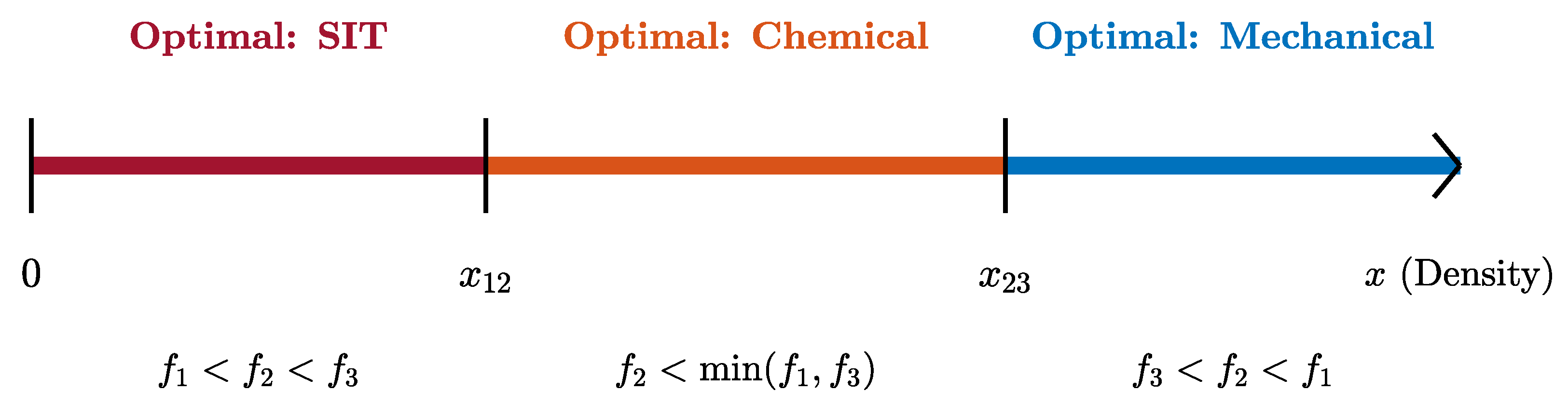
$x_{12}^{\ast }<x_{23}^{\ast }$ (Complete Three-Stage Hierarchy) (Figure 1)

This corresponds to a parameter regime where all three strategies have their dominant intervals.

Low density ($0<x<x_{12}^{\ast }$): $f_1\left(x\right)<f_2\left(x\right)<f_3\left(x\right)$. SIT induces the Allee effect and is the effective strategy for eradication.

Intermediate density ($x_{12}^{\ast }<x<x_{23}^{\ast }$): $f_2\left(x\right)<min(f_1\left(x\right),f_3\left(x\right))$. Chemical control provides the strongest suppression due to its direct mortality impact.

High density ($x>x_{23}^{\ast }$): $f_3\left(x\right)<f_2\left(x\right)<f_1\left(x\right)$. Mechanical habitat reduction dominates by explicitly truncating the system’s capacity.

(2) 

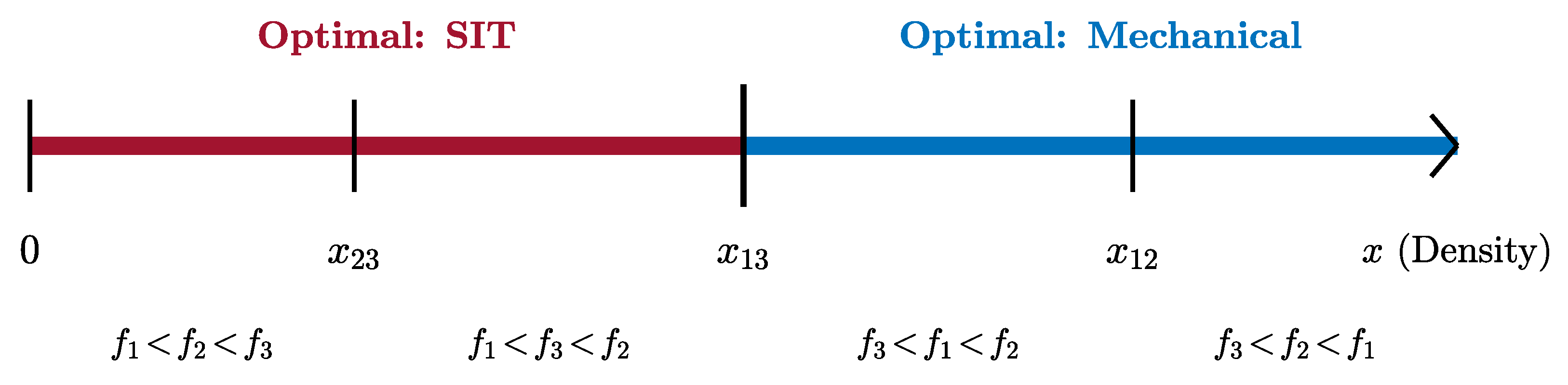
$x_{12}^{\ast }>x_{23}^{\ast }$ (Two-Stage Dominated Hierarchy) (Figure 2)

When the chemical killing rate, $\sigma$, is relatively weak or the SIT efficacy, r, is extremely high, the structural thresholds cross, leading to the collapse of the chemical dominance interval:

Low density ($0<x<x_{23}^{\ast }$): $f_1\left(x\right)<f_2\left(x\right)<f_3\left(x\right)$. SIT remains the effective strategy.

Intermediate density ($x_{23}^{\ast }<x<x_{12}^{\ast }$): In this regime, both mechanical removal and SIT outperform chemical control ($f_3<f_2$ and $f_1<f_2$). Chemical intervention becomes strictly inferior. The effective strategy transitions directly from SIT to mechanical removal at the root, $x_{13}^{\ast }$.

High density ($x>x_{12}^{\ast }$): $f_3\left(x\right)<f_2\left(x\right)<f_1\left(x\right)$. Mechanical removal remains effective.

Solving these inequality boundaries indicates the dependence of control strategies on mosquito population size.

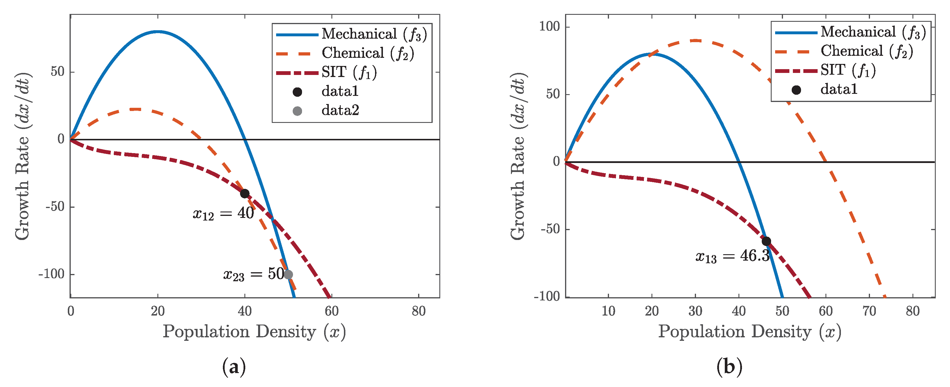
We conduct a geometric comparison of the growth rate functions corresponding to the three control strategies under different parameter regimes (Figure 3).

Case A ($x_{12}^{\ast }<x_{23}^{\ast }$): With a strong chemical killing rate ($\sigma =0.5$), the density axis is partitioned into three regimes where SIT, chemical, and mechanical methods sequentially dominate the suppression rate.

Case B ($x_{12}^{\ast }>x_{23}^{\ast }$): With a weaker chemical killing rate ($\sigma =0.2$), the chemical growth rate ($f_2$) is strictly dominated by the other two strategies. The effective efficiency transitions directly from SIT to mechanical removal at the root, $x_{13}^{\ast }\approx 46.6$.

For mechanical removal and chemical control, the growth rate curves $f_2\left(x\right)$ and $f_3\left(x\right)$ maintain the shape of an inverted parabola. As long as the intrinsic growth rate is positive (i.e., $b-\delta >0$ or $b-\delta -\sigma >0$), the curve intersects the x-axis at a single stable positive point. This implies that these two strategies are monostable systems: the population converges monotonically to a new equilibrium without any “extinction trap”.

In contrast, the SIT strategy introduces a non-monotonic nonlinearity, ${\displaystyle \frac{x}{x+r}}$. When $0<R<R_{crit}$, the system exhibits bistability (the coexistence of a stable positive equilibrium and a stable extinction equilibrium), a feature absent in physical and chemical methods. Furthermore, when the release number, R, exceeds a critical value, $R_{crit}$, the non-trivial intersection between the growth curve and the axis disappears, and the system transitions to a monostable state where $x=0$ becomes the unique global attractor, providing a theoretical possibility for complete eradication.

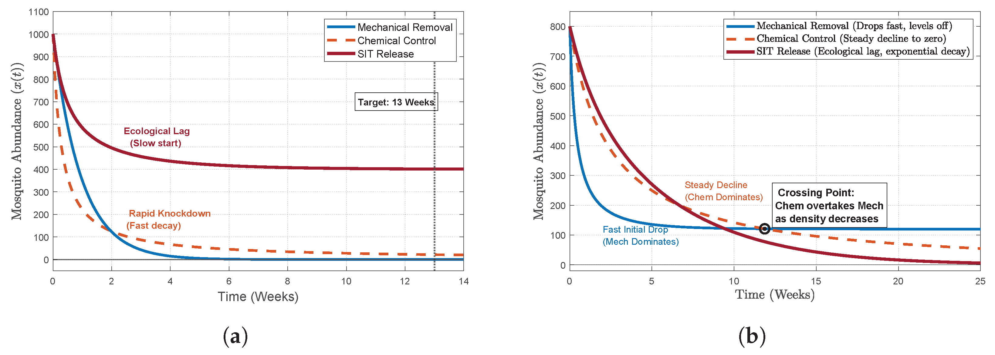
We further analyze the time–response characteristics of the controls. Numerical simulations reveal distinct temporal pathways for the three strategies (see Figure 4).

Chemical control acts directly on the linear mortality term, $-\sigma x$, yielding instantaneity, where the population density drops exponentially.

Table 1. Pairwise comparison of suppression efficiency across density regimes.

Compared Pairs	Critical Threshold (${\mathit{x}}_{\mathit{crit}}$)	$\mathit{x}<{\mathit{x}}_{\mathit{crit}}$	$\mathit{x}>{\mathit{x}}_{\mathit{crit}}$
S2 ($f_2$) vs. S3 ($f_3$)	$x_{23}^{\ast }={\displaystyle \frac{\sigma }{(\theta -1)\varphi }}$	$f_2<f_3$	$f_3<f_2$
S1 ($f_1$) vs. S2 ($f_2$)	$x_{12}^{\ast }={\displaystyle \frac{r(b-\sigma )}{\sigma }}$	$f_1<f_2$	$f_2<f_1$
S1 ($f_1$) vs. S3 ($f_3$)	$x_{13}^{\ast }$ (root of $g\left(x\right)=0$)	$f_1<f_3$	$f_3<f_1$

compares mosquito population suppression speeds under different conditions, suggesting that the selection of a single strategy requires careful consideration of local environmental conditions.

3. Setting a Buffer Area to Control Migratory Mosquitoes

The dynamical analysis in Section 2 assumes that mosquitoes live in a closed area. In practical applications, however, the treated area is inevitably subject to the migration of wild mosquitoes from untreated surroundings. This constant migration destroys the ideal extinction equilibrium ($x=0$), leading to mosquito population resurgence. Consequently, the temporal dynamics model alone is insufficient. To maintain a low population density in the protected area, we extend the framework to a one-dimensional spatial model and design a “buffer zone” to offset external invasion.

3.1. Wild Mosquitoes Enter the Protected Area Naturally (From Wild to Internal Protected Area)

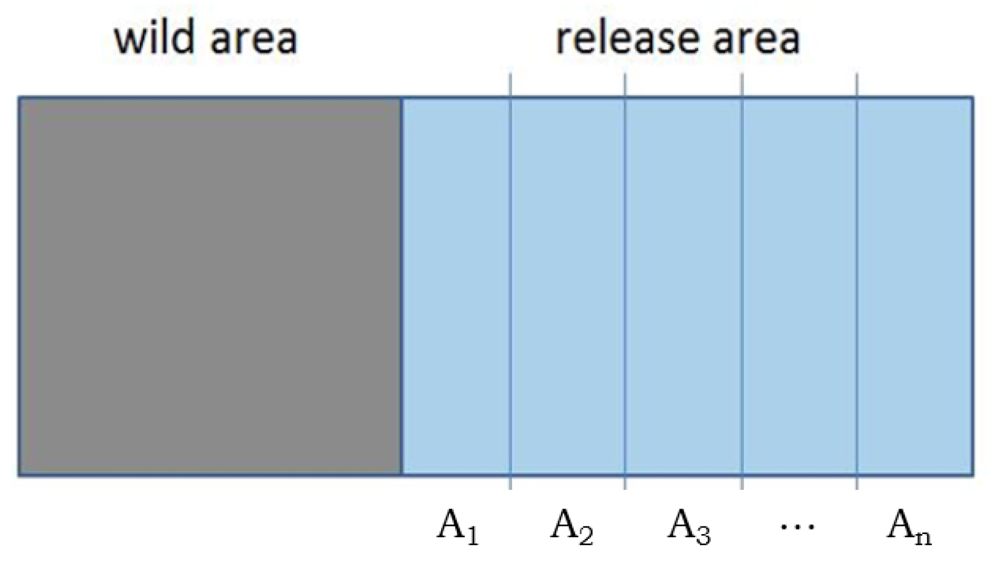
We divide the release area (buffer area and protected area) into N small parts of rectangular shape and let the width of these rectangles be constant at L, say 30 m. Let $A_i$, $i=1,2,\cdots ,N$ denote the N sub-areas from the boundary of the wild area and the release area (see Figure 5).

We first discuss the situation in which one boundary of the release area is in natural isolation, as in Figure 5. In [26,27], the authors employed simple oviposition traps, captured adult female Ae. aegypti across high-rise apartment blocks and genotyped them using genome-wide SNP markers. They found that the mean effective dispersal distance was estimated at 45.2 m (95% CI 39.7–51.3 m), with a 10% probability of a dispersal distance greater than 100 m (95% CI 92–117 m). In addition, in our field trial [11], the field workers also believed that most mosquitoes stay near their breeding grounds.

To mathematically formalize the spatial diffusion of mosquitoes, we define a discretized probability kernel based on the empirical data from [26]. Filipović et al. [26] estimated a mean effective dispersal distance of 45.2 m and an approximate 10% probability of long-distance dispersal.

Assuming a symmetric random walk over a standardized biological time step, the diffusion kernel maps to our grid ($L=30$ m) as follows: the probability of a mosquito remaining in its current patch, $A_i$ (a range of $[-15\mathrm{m},15\mathrm{m}]$ from the center), is set to ${\alpha }_0=0.5$. The probability of moving to the immediately adjacent patches, $A_{i\pm 1}$ (approximately 30 m away), is ${\alpha }_1=0.2$ in each direction.

To account for the observed long-distance dispersal tail, the probability of reaching $A_{i\pm 2}$ (approximately 60 m away) is assigned as ${\alpha }_2=0.05$ for each direction. We omit the case in which mosquitoes move to farther areas.

This configuration rigorously satisfies the probability conservation (${\alpha }_0+2{\alpha }_1+2{\alpha }_2=1$). More importantly, under this probability mass function, the expected dispersal distance per time step is $\mathbb{E}\left[\right|X\left|\right]=0\left({\alpha }_0\right)+30\left(2{\alpha }_1\right)+60\left(2{\alpha }_2\right)=18$ m.

Accumulated over a typical mosquito active lifespan (roughly 2.5 time steps), this mathematically yields a lifetime mean dispersal of 45 m, closely matching the empirical 45.2 m [26]. Furthermore, the exact 10% tail probability ($2{\alpha }_2=0.10$) seamlessly captures the long-distance migration characteristics.

To formulate the spatial model as a true continuous-time dynamic system, we transform the discrete probabilities into continuous migration rates. Let $m_1=0.2$ and $m_2=0.05$ represent the continuous diffusion rates to the immediately adjacent and next-adjacent patches, respectively. We apply a continuous source boundary condition on the left interface (the untreated wild area with a constant mosquito abundance, $y_0$) and a zero-flux (reflecting) boundary condition on the right interface (the core protected area), assuming mosquitoes cannot migrate beyond the defined boundary, $A_N$.

Following the ideas in [19,28], we let $x_i\left(t\right)$ denote the mosquito abundance (the total number of mosquitoes) in patch $A_i$ at time t. To maintain dimensional consistency between abundance and carrying capacity, we assume all patches have an identical area of $30\mathrm{m}\times L_w$, where $L_w$ is the standardized length of the buffer strip. Accordingly, all state variables, boundary sources, and carrying capacities are uniformly expressed in terms of abundance per patch. By decoupling the local population growth, $f_1\left(x_i\right)$, under the SIT intervention from the spatial Laplacian-type diffusion terms, we establish the following patch-based ordinary differential equations (ODEs):

$$\left\{\begin{array}{c}{\displaystyle \frac{\mathrm{d}{x}_1\left(t\right)}{\mathrm{d}t}=f_1\left(x_1\right)+m_1(y_0-2x_1+x_2)+m_2(y_0-2x_1+x_3),}\hfill \\ {\displaystyle \frac{\mathrm{d}{x}_2\left(t\right)}{\mathrm{d}t}=f_1\left(x_2\right)+m_1(x_1-2x_2+x_3)+m_2(y_0-2x_2+x_4),}\hfill \\ {\displaystyle \frac{\mathrm{d}{x}_i\left(t\right)}{\mathrm{d}t}=f_1\left(x_i\right)+m_1(x_{i-1}-2x_i+x_{i+1})+m_2(x_{i-2}-2x_i+x_{i+2}),2<i<N-1,}\hfill \\ {\displaystyle \frac{\mathrm{d}{x}_{N-1}\left(t\right)}{\mathrm{d}t}=f_1\left(x_{N-1}\right)+m_1(x_{N-2}-2x_{N-1}+x_N)+m_2(x_{N-3}-x_{N-1}),}\hfill \\ {\displaystyle \frac{\mathrm{d}{x}_N\left(t\right)}{\mathrm{d}t}=f_1\left(x_N\right)+m_1(x_{N-1}-x_N)+m_2(x_{N-2}-x_N),}\hfill \end{array}\right.$$

(13)

where $f_1\left(x\right)$ is defined in (2). This patch-based ODE system provides a rigorous mathematical foundation for evaluating the spatiotemporal invasion dynamics within the buffer zone.

To strictly justify the mathematical foundation of the spatial model, we establish the following theoretical results regarding the positivity, boundedness, and stability of the system.

Theorem 1 

(Positivity and Boundedness). For any non-negative initial condition, $x\left(0\right)\in {\mathbb{R}}_{+}^N$, the patch-based ODE system admits a unique solution, $x\left(t\right)$, that remains non-negative for all $t>0$. Furthermore, the solutions are uniformly bounded, i.e., there exists a positive constant, $M>0$, such that ${lim\; sup}_{t\to \infty }{x}_i\left(t\right)\le M$ for all $i=1,2,\dots ,N$.

Proof. 

First, we demonstrate the positivity. For any patch, i, if $x_i=0$ while all other state variables remain non-negative, the intrinsic growth term is $f_1\left(0\right)=0$. Consequently, the derivative is solely determined by the influx from adjacent patches and the external boundary: ${\displaystyle \frac{\mathrm{d}{x}_i}{\mathrm{d}t}}{|}_{x_i=0}\ge m_1(x_{i-1}+x_{i+1})+m_2(x_{i-2}+x_{i+2})\ge 0$. Since the vector field on the boundary of the positive orthant, ${\mathbb{R}}_{+}^N$, points strictly inward or is tangent to the boundary, the non-negative orthant is a positively invariant set. Second, to prove boundedness, note that the intrinsic growth function is upper-bounded by the standard logistic growth: $f_1\left(x\right)\le (b-\delta )x-\varphi x^2$. Let $K=(b-\delta )/\varphi$ denote the natural carrying capacity without SIT intervention. Define a uniform upper bound, $M=max\{y_0,K\}$. Suppose there exists a time, $t_0$, and a patch, i, such that $x_i\left(t_0\right)\ge M$ achieves the maximum across all spatial patches. Since $x_i$ is the spatial maximum, the discrete Laplacian-type diffusion terms are non-positive. Concurrently, since $x_i\ge K$, $f_1\left(x_i\right)<0$. Therefore, ${\displaystyle \frac{\mathrm{d}{x}_i}{\mathrm{d}t}}{|}_{t_0}<0$. By the comparison principle, the population density in any patch cannot indefinitely exceed M. □

Theorem 2 

(Asymptotic Behavior and Stability). The spatial buffer zone model is a cooperative dynamical system. Every bounded non-negative solution converges asymptotically to a steady-state equilibrium, guaranteeing the existence of a stable spatial invasion profile.

Proof. 

We evaluate the Jacobian matrix, $J=\left({\displaystyle \frac{\partial {\dot{x}}_i}{\partial x_j}}\right)$, of the ODE system. For any $i\ne j$, the off-diagonal elements consist exclusively of the diffusion coefficients $m_1$ and $m_2$. Since $m_1>0$ and $m_2>0$, all off-diagonal entries are non-negative (${\displaystyle \frac{\partial {\dot{x}}_i}{\partial x_j}}\ge 0$ for $i\ne j$). This structural property defines a strictly cooperative (quasi-monotone) system. According to the Hirsch theory of monotone dynamical systems, the bounded orbits of a strongly cooperative system generically converge to the set of equilibria. Therefore, the spatial invasion wave will not oscillate indefinitely but will stabilize into a steady-state profile. □

Now we consider the design of the buffer area. While Section 2 utilized normalized parameters for qualitative topological analysis, here we adopt a set of scaled empirical parameters to better capture the actual demographic scale and spatial diffusion dynamics in a multi-patch environment. Specifically, considering the environmental carrying capacity, $K\approx \mathrm{136,470}$, calculated from the biological parameters, we set $N=10$. To distinguish between the boundary condition and the initial states, we set the constant external boundary source as $y_0=\mathrm{136,000}$. For the initial conditions of the spatial patches at $t=0$, we assume the first patch is fully invaded, setting $x_1\left(0\right)=\mathrm{136,000}$, while the remaining patches are initially free of mosquitoes, setting $x_i\left(0\right)=0$ for $i=2,3,\dots ,10$. Based on the data in [18,20,29], we take $b=1.3$, $\delta =0.14$, and $\varphi =8.5\times {10}^{-6}$.

It is important to clarify that K and $y_0$ here do not represent the absolute physical density strictly confined to a single $30\mathrm{m}\times 30\mathrm{m}$ patch, which would be biologically unrealistic. Instead, they serve as scaled regional aggregate parameters representing the total population flux along the entire extended length of the boundary strip. This scaling preserves the qualitative spatiotemporal threshold dynamics and structural ratios of the multi-patch system, ensuring the numerical stability of the continuous ODE framework while aligning with the theoretical literature.

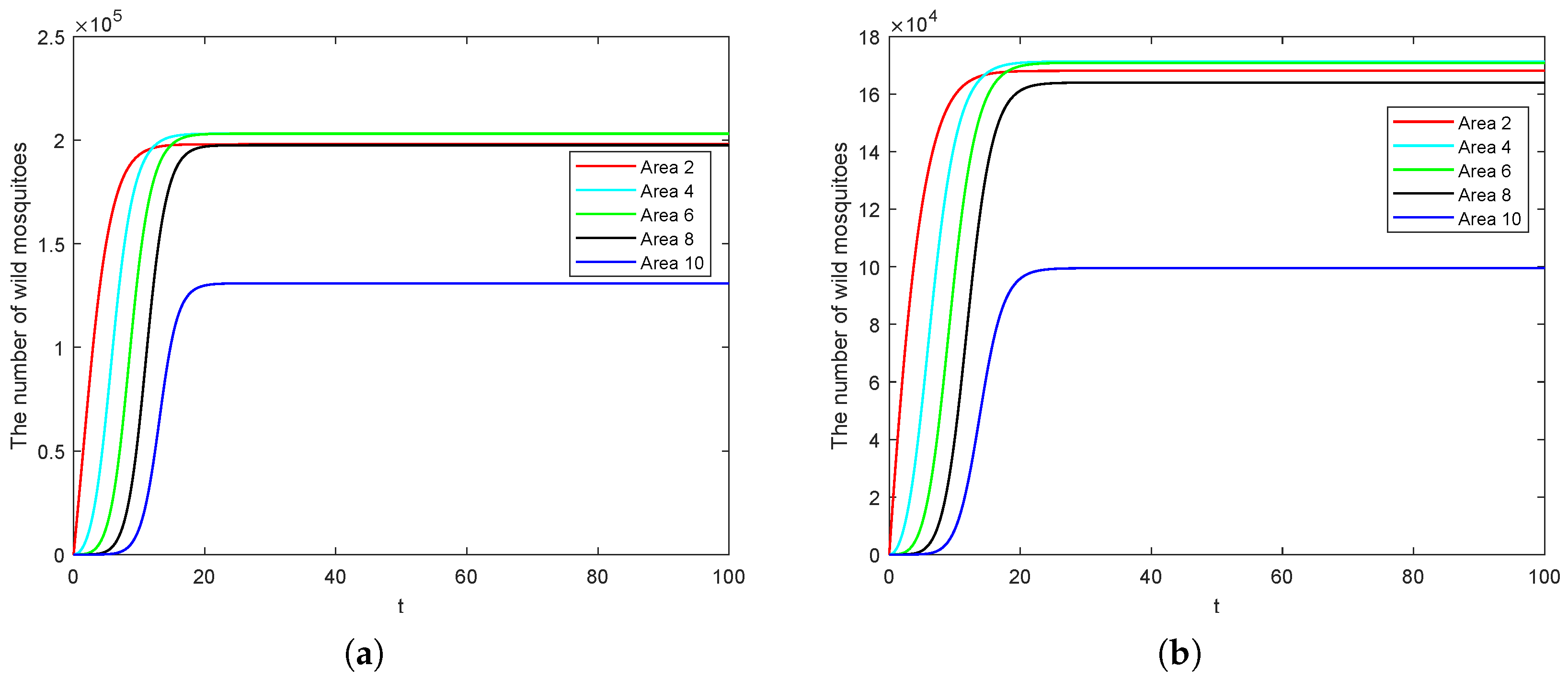
As shown in Figure 6, a higher release amount of sterile mosquitoes ($R=\mathrm{100,000}$) suppresses the population significantly faster and achieves a lower equilibrium across all buffer regions compared to the baseline release ($R=\mathrm{50,000}$).

However, if $y_0$ increases to 200,000, the demand for sterile male mosquitoes will increase. Here, we consider combining two suppression schemes in the buffer zone.

As observed in Figure 7, under higher invasion pressure, combining SIT with pesticides (S1 + S2) provides a faster initial knockdown effect, whereas combining SIT with mechanical clearance (S1 + S3) ensures a lower and more stable long-term density in the buffer patches.

Next, we will consider a case in which the three control methods are used simultaneously.

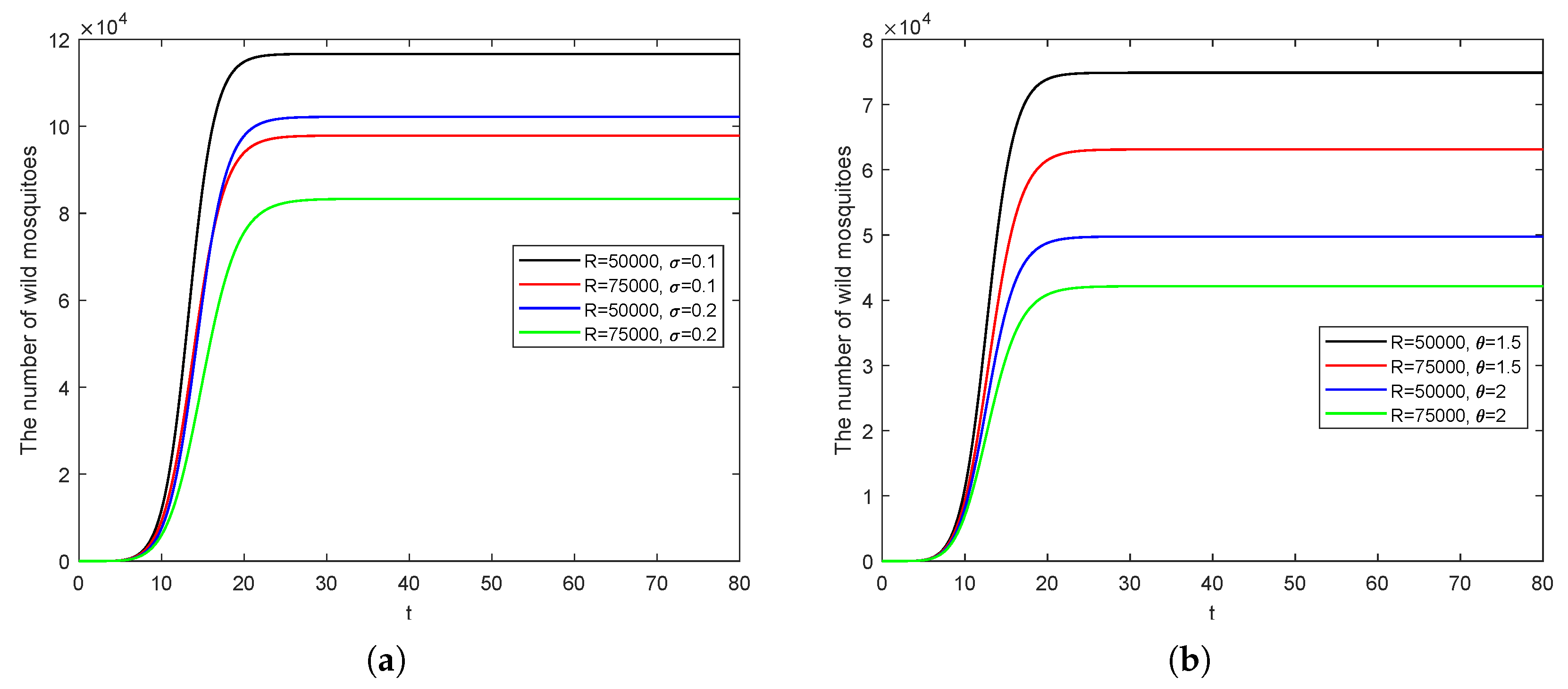
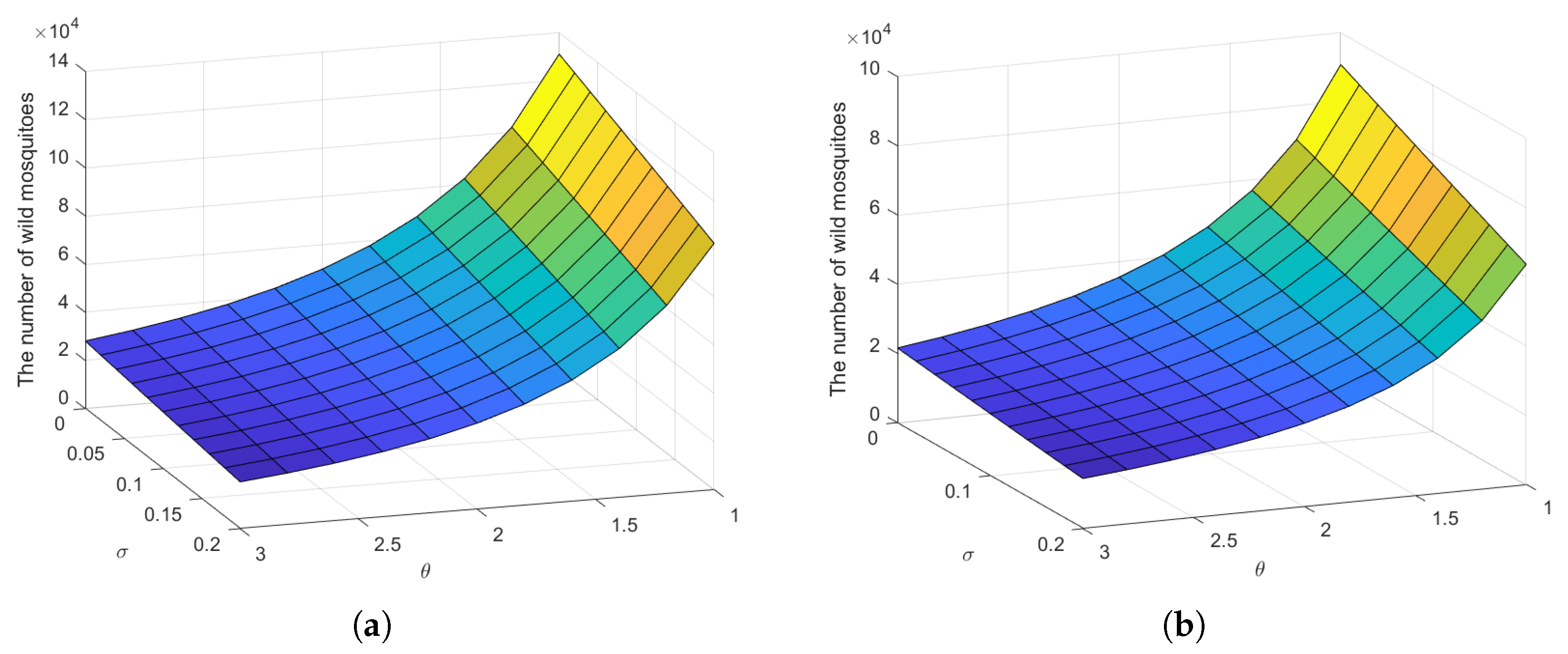
Figure 8 demonstrates that, when all three strategies are employed simultaneously, the suppression effect is highly robust. Increasing the mechanical clearance factor ($\theta$) or chemical killing rate ($\sigma$) drastically enhances the overall efficacy, establishing a robust barrier in the buffer zone.

The key question for the buffer area is whether the wild mosquitoes can migrate to the protected area with a given initial quantity. Based on the above discussions, the problem can be reformulated to determine how wild mosquitoes spread in the release area under suppression over time. We consider two cases for the release area.

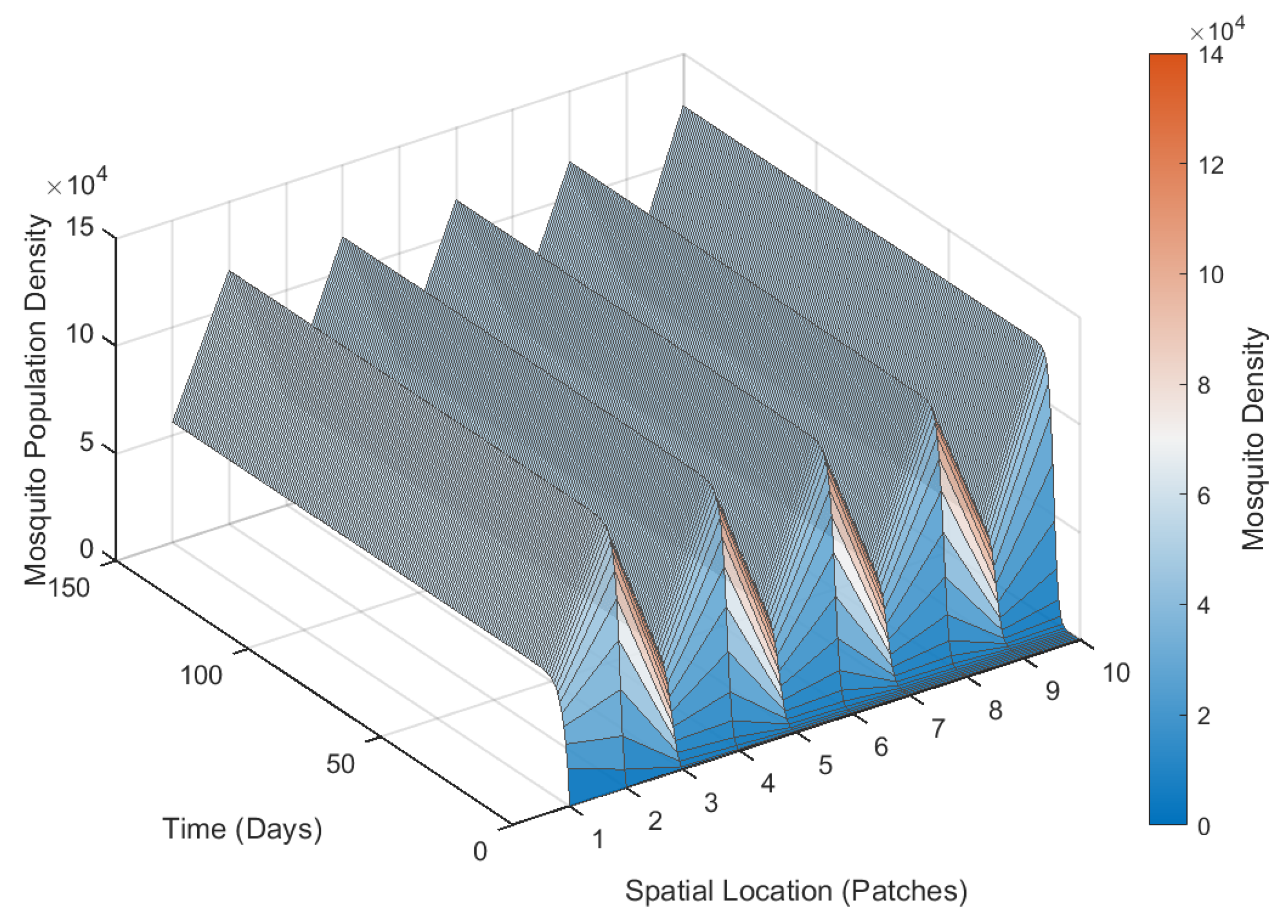
Case 1: Insufficient Buffer Width and Fragmented Distribution. When the number of spatial patches, N, is small (e.g., $N<10$), or when the suppression interventions are deployed in a fragmented, discontinuous manner due to practical constraints, the “stepping-stone effect” becomes highly significant. Wild mosquitoes from the continuous external source ($y_0$) exploit the untreated or weakly suppressed adjacent patches as ecological refuges. These untreated patches act as stepping-stones, allowing the mosquito population to rapidly recover and form a sawtooth-like spatiotemporal invasion pattern (see Figure 9). Consequently, the fragmented suppression is easily bypassed by the cumulative invasion flux, leading to a failure in maintaining the mosquito-free status in the core protected area ($A_N$). This suggests that a continuous, sufficiently wide buffer zone is crucial to truncate the invasion.

Case 2: Effective Buffer Width.

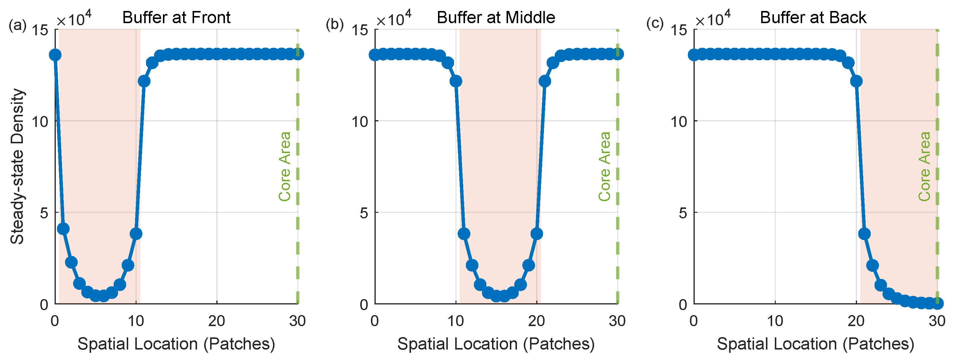
Before determining the required width of the buffer zone, we first evaluate its effective spatial placement relative to the core area. As explicitly demonstrated in the 2D steady-state spatial profiles (see Figure 10), the population dynamics exhibit marked topological differences across the three deployment strategies.

• Buffer at the front (left panel): While placing the buffer at the outer boundary truncates the initial invasion source (dropping the density from 136,000 to near 0), it leaves a vast spatial domain ($A_{11}$ to $A_{30}$) completely unmanaged. Although the steady-state density remains low in this scenario, this vast unprotected rear area is ecologically fragile and highly vulnerable to secondary outbreaks if any internal human-induced introductions occur.
• Buffer in the middle (center panel): This strategy completely fails to protect the core. The external mosquitoes fully infest the front patches ($A_1$ to $A_{10}$). Although the middle buffer temporarily suppresses the density, the unsuppressed patches behind the buffer ($A_{21}$ to $A_{30}$) allow the surviving mosquitoes to rapidly rebound to the environmental carrying capacity ($K\approx \mathrm{136,470}$) via logistic growth, leaving the core area fully compromised.
• Buffer at the back (right panel): Anchoring the buffer strictly adjacent to the core area serves as the important final layer of protection. As the curve shows, even when the external invasion completely floods the outer and middle patches (maintaining a high density of 136,000), the localized, high-intensity suppression immediately surrounding the core forces a precipitous drop in mosquito density.

To quantify the relationship between buffer size and protection efficiency, we simulated the equilibrium density of mosquitoes in the furthest protected area ($A_N$) under varying buffer widths.

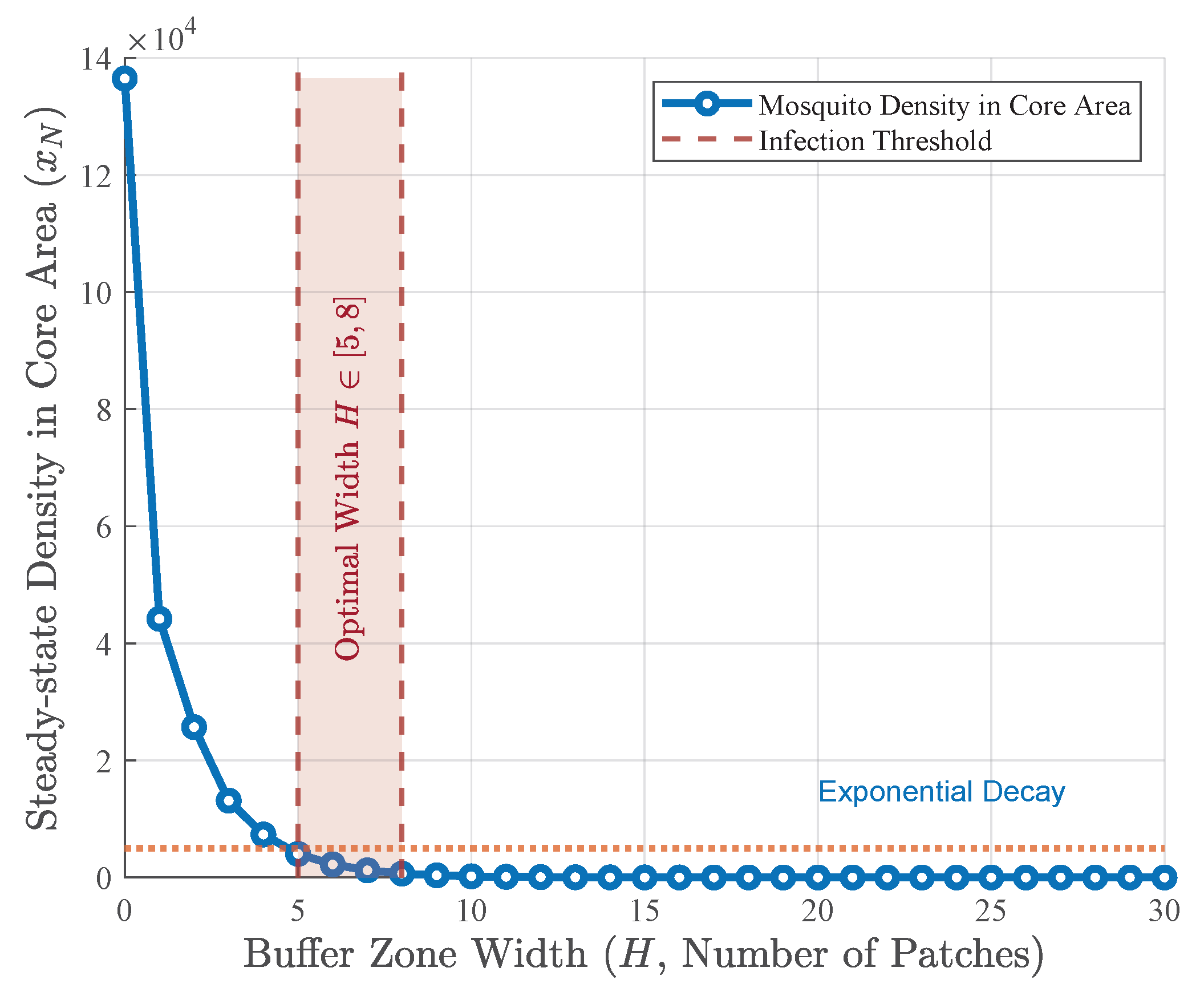
As shown in Figure 11, the mosquito density exhibits an exponential decay as the buffer width increases. The results indicate that a buffer zone of 5–8 patches provides the effective trade-off between cost and safety. When $N\ge 5$, the invasion wave is effectively pinned, and the density in the core area converges to near zero. Further increasing the width yields diminishing marginal returns.

Therefore, establishing a buffer zone of 5–8 patches is identified as the critical spatial condition for blocking the invasion channel in an open system.

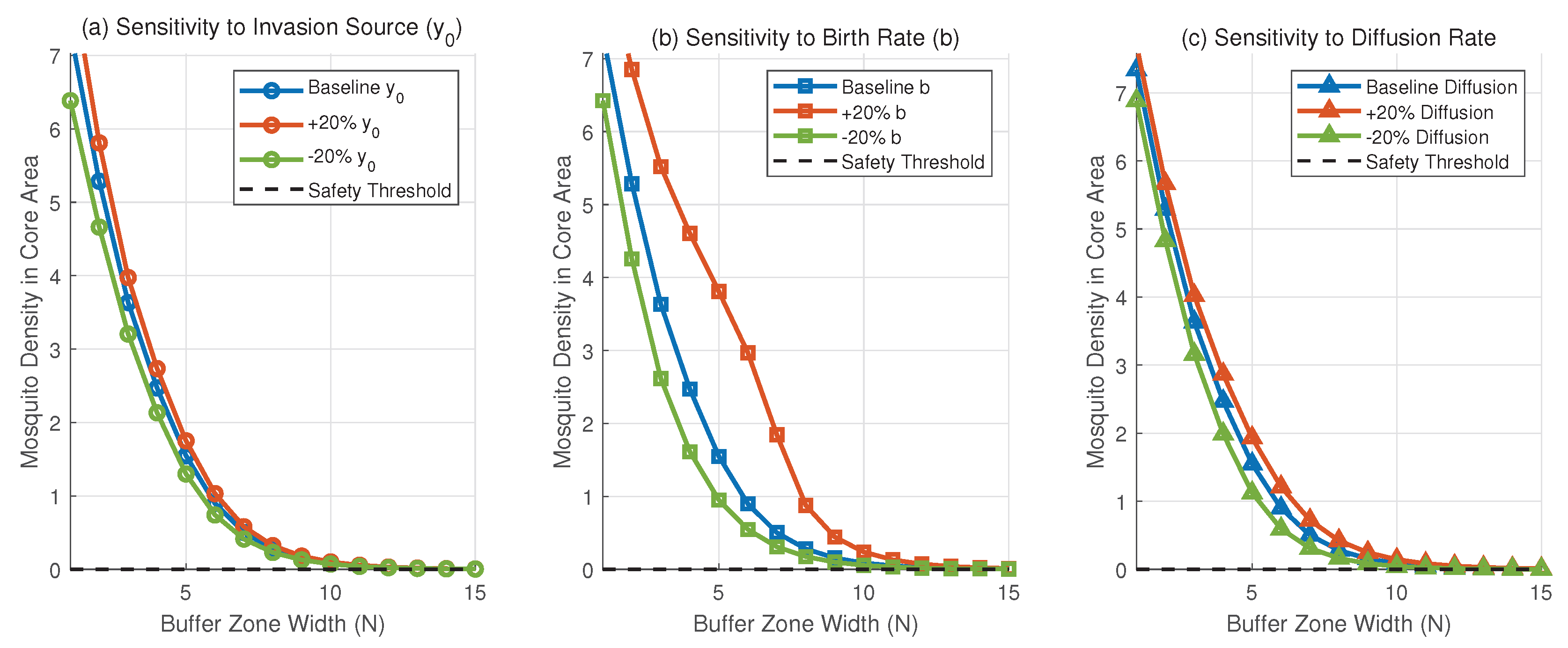
To verify the robustness of our conclusion regarding the buffer zone size, we performed a single-factor sensitivity analysis. The stability of the spatial control strategy could be affected by environmental fluctuations, such as variations in the external invasion source ($y_0$), the intrinsic birth rate of mosquitoes (b), and the mosquitoes’ diffusion capabilities. Therefore, we independently perturbed these three key parameters by $\pm 20\%$ to observe whether the effective buffer width remains consistent.

As illustrated in Figure 12, while the absolute equilibrium density in the front patches varies, the overall topological structure of the exponential decay remains stable. The system exhibits high robustness to variations in the external invasion source, $y_0$ (Figure 12a), and spatial diffusion rates (Figure 12c), where the required buffer width to reach the safety threshold ($x_N\le 20$) slightly shifts to approximately 9–10 patches under a $+20\%$ perturbation. However, the system is notably more sensitive to the intrinsic birth rate, b (Figure 12b). A $+20\%$ increase in the birth rate extends the required buffer width to approximately 13–14 patches to successfully pin the invasion wave. This analysis mathematically confirms that, while a standard 5–8-patch buffer is effective under baseline conditions, precise environmental assessment of the local mosquito reproduction rate is critical in field applications, as higher birth rates necessitate wider buffer zones to maintain an effective barrier.

3.2. Cleaning Up Breeding Sites to Reduce the Mosquito Population

Before implementing high-cost interventions like SIT, reducing the environmental capacity (K) through source reduction can significantly lower the critical release threshold required for SIT, acting as a highly effective complementary strategy. Unlike chemical pesticides that temporarily increase mortality rate ($\sigma$), cleaning breeding sites permanently lowers the carrying capacity of the habitat, $K_{new}=K/\theta$, where $\theta >1$ is the clearance intensity factor. Our simulation highlights two distinct advantages of this mechanical approach.

First, it acts as a “bottom-up” suppression. By reducing K, we lower the baseline population density, thereby reducing the critical release threshold ($R_{crit}$) required for SIT to be effective in subsequent stages.

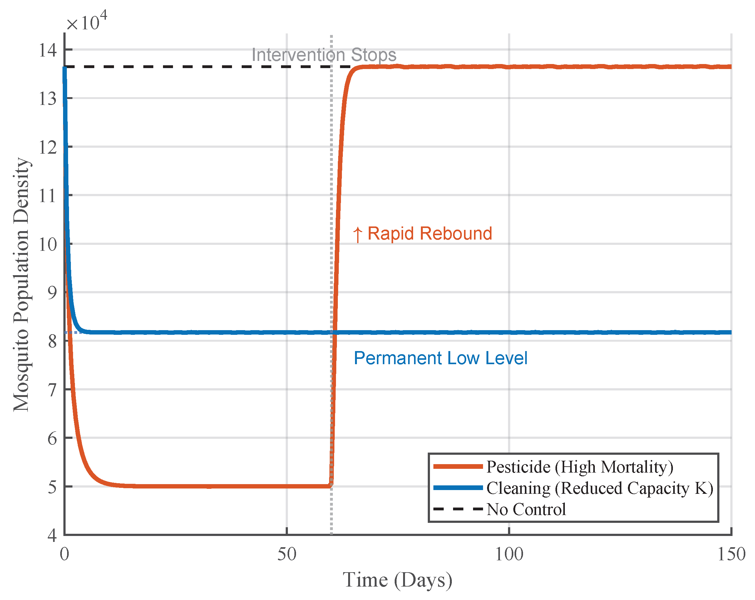
Second, source reduction enhances the resilience of the control. As shown in Figure 13, while pesticide application yields a rapid initial decline, the population rebounds swiftly to the original level once spraying ceases.

To compare resilience, the chemical killing rate, $\sigma$, is independently calibrated to suppress the equilibrium density to 50,000 before interventions are halted. Both interventions are halted at $t=60$ days.

In contrast, cleaning breeding sites leads to a moderate but irreversible decline. Even if the intervention is interrupted, the population is constrained by the reduced $K_{new}$, preventing a full-scale resurgence. Therefore, cleaning breeding sites serves as the prerequisite for destabilizing the vector population before deploying SIT.

3.3. Rational Use of Pesticides

Compared to the release of Wolbachia-infected sterile male mosquitoes, the use of pesticides can drastically reduce the wild mosquito population in a short time. Therefore, complementary to biological suppression, chemical intervention provides a mechanism to explicitly truncate the invasion flux. However, the rational use of pesticides is crucial to minimize environmental impact and manage insecticide resistance. Assuming the wild area acts as a continuous source of susceptible mosquitoes and migration is primarily unidirectional into the release area, the selection pressure for resistance can be diluted if insecticide application is spatially restricted.

This raises several critical spatial optimization questions:

(1)

Should pesticides be applied uniformly or restricted to specific designated areas?

(2)

How can we minimize pesticide usage while guaranteeing suppression efficacy?

(3)

Should pesticides be applied continuously or periodically?

(4)

Is it more efficient to target the boundary area where the mosquito density is the highest?

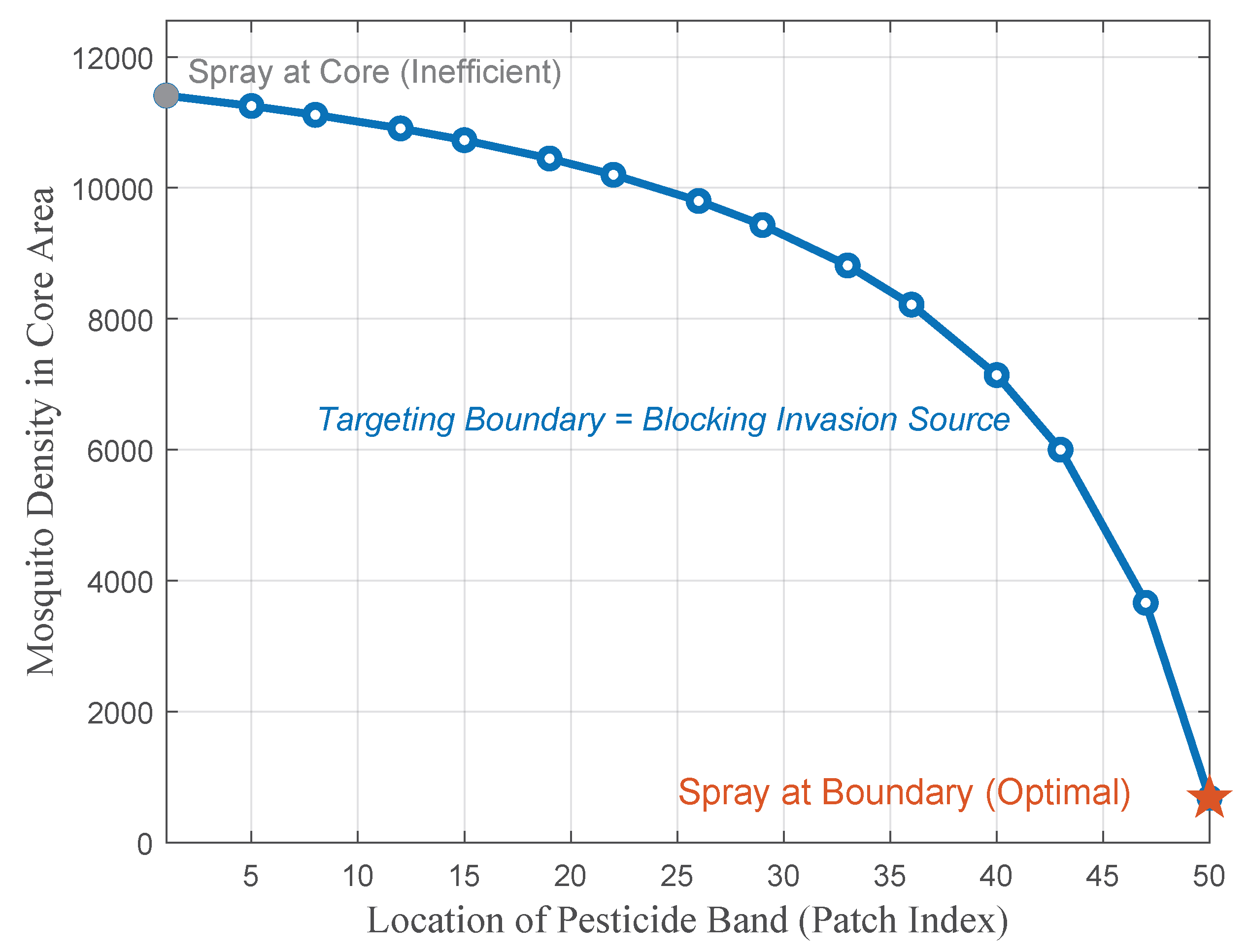
To address these questions and identify an effective spatial layout, we simulated the suppression efficiency under different pesticide application scenarios (see Figure 14). To evaluate the spatial placement of the pesticide application with a higher resolution and observe a continuous efficacy gradient, we temporarily expanded the spatial domain to $N=50$ patches for this specific set of simulations.

• Effective location: The simulation clearly demonstrates that deploying pesticides at the boundary (high-density interface) is significantly more efficient than deploying them in the middle or core areas. As shown in Figure 14, shifting the spraying zone from the core ($i=1$) to the boundary ($i=N$) results in a monotonic decrease in the final mosquito density in the protected area.

A fixed-intensity pesticide band (spanning one patch width) is applied at location i, and its position is evaluated from the core ($i=1$) to the boundary ($i=50$).

This is because the boundary acts as the “source” of invasion. Spraying at the source maximizes the “kill-per-unit” efficiency due to the density-dependent nature of the encounter rate, effectively acting as a “Chemical Firewall” that truncates the invasion flux before it spreads.

2.

Continuous vs. periodic: While periodic spraying can reduce chemical usage, our results (refer to Figure 12 in Section 3.1) indicate that it creates “windows of opportunity” for rapid population rebound, especially when the external mosquito source, $y_0$, remains high. Therefore, to maintain a robust “Firewall” at the boundary, continuous suppression (or high-frequency pulses) is recommended to prevent the “stepping-stone” breach.

3.

Resistance Management: By confining the high-intensity chemical suppression strictly to the boundary (a narrow band), the inner buffer zone serves as a “spatial refugium” where no pesticides are used. This spatial heterogeneity allows susceptible genes to persist in the buffer zone (albeit at low density), diluting the selection pressure for resistance, consistent with the hypothesis that a loss of resistance occurs in the absence of constant exposure.

4. Discussion

There have been many studies on maintaining the ecological security of protected areas by establishing buffer zones [12,13,14]. In this work, we discuss the setup of buffer zones to prevent external mosquito vectors from invading the protected area and disrupting the suppression effect. Most existing studies consider the continuous dispersal of mosquitoes and have established diffusion models to characterize invasion processes; such approaches perform well in environments with uniformly distributed terrain and buildings. In reality, however, the terrain surrounding protected areas is not necessarily continuous—for instance, green belts and residential areas may be intermingled in some regions—making spatially discrete and temporally continuous models more suitable for capturing real-world conditions. In addition, if human intervention measures such as insecticide spraying are carried out in localized areas, the patch model is also relatively easy to handle. In this work, we assume that mosquito vectors in both the protected area and its surrounding regions have already been reduced to a low density through prior intensive suppression, and that continued high-intensity suppression can maintain the effect, but at a high control cost. We therefore consider that establishing a buffer zone with relatively low-dose control can sustain the suppression effect.

In addition to considering the release of sterile male mosquitoes as the primary measure, we also discussed the appropriate combination of two supplementary approaches—source reduction (eliminating breeding sites) and insecticide spraying—and examined how we might improve suppression efficacy, with the relevant conclusions derived through simulation. Following the approach outlined in [19,28], we divided the buffer zone into adjacent discrete regions and considered a simple diffusion scenario, namely the unidirectional dispersal of external mosquito vectors from one side to the other. In this context, we examined the relationship between control measures and the resulting suppression effect. In future work, we plan to consider more general geometric configurations of the buffer zone and multiple pathways of mosquito invasion.

The conclusions in [16] and our numerical simulation results all demonstrate the dependence of the suppression effect on spatial location and time. For cases with uneven terrain distribution, we can set the corresponding reproduction parameters and diffusion coefficients according to specific conditions, although we do not perform simulations for such cases in this paper. The authors of [15] mainly considered the case of two patches and reveal the rich dynamic behaviors of mosquito-borne suppression. Based on our discussion of the multi-patch scenario, the system has multiple equilibria for given parameters, and when the initial state falls into the corresponding attraction domain, the solution will approach the corresponding equilibrium.

References

1. Calisher, C.H. Persistent emergence of dengue. Emerg. Infect. Dis. 2005, 11, 738–739. [Google Scholar] [CrossRef] [Scilit]
2. Kyle, J.L.; Harris, E. Global spread and persistence of dengue. Annu. Rev. Microbiol. 2008, 62, 71–92. [Google Scholar] [CrossRef] [Scilit] [PubMed]
3. Long, J.; Lin, B.; Zhang, P.; Xue, J.; Ma, Y.; Chen, F.; Li, F. Analysis on the epidemiological characteristics of dengue fever in Guangdong province. China Med. Pharm. 2015, 5, 183–185. (In Chinese) [Google Scholar]
4. Dai, B.; Liu, W.; Zhen, R.; Zhang, W.; Lu, Y.; Liu, Y. Epidemiological characteristics of dengue fever in Guangzhou City in 2024. Chin. J. Schistosomiasis Control 2025, 37, 549–554. [Google Scholar] [CrossRef] [Scilit] [PubMed]
5. William, M.; Marc, L.; Scott, C.W. Chikungunya virus and other emerging arthritogenic alphaviruses. Naturerev. Microbiol. 2025, 23, 585–601. [Google Scholar] [CrossRef] [Scilit] [PubMed]
6. Zhang, M.; Li, Y.; Huang, X.; Liu, M.; Jiang, S.; Zeng, B.; Ouyang, L.; Huang, J.; Mai, B.; Guan, Q.; et al. Epidemiological characteristics and transmission dynamics of the early stage Chikungunya fever outbreak in Foshan City, Guangdong Province, China in 2025. Infect. Dis. Poverty 2025, 14, 93. [Google Scholar] [CrossRef] [Scilit] [PubMed]
7. Ooi, E.E.; Goh, K.T.; Gubler, D.J. Dengue prevention and 35 years of vector control in Singapore. Emerg. Infect. Dis. 2006, 12, 887–893. [Google Scholar] [CrossRef]
8. Gándara, L.; Jacoby, R.; Laurent, F.; Spatuzzi, M.; Vlachopoulos, N.; Borst, N.O.; Ekmen, G.; Potel, C.M.; Garrido-Rodriguez, M.; Böhmert, A.L.; et al. Pervasive sublethal effects of agrochemicals on insects at environmentally relevant concentrations. Science 2024, 386, 446–453. [Google Scholar] [CrossRef] [Scilit] [PubMed]
9. Hoffmann, A.A.; Turelli, M. Cytoplasmic incompatibility in insects. In Influential Passengers: Inherited Microorganisms and Arthropod Reproduction; O’Neill, S.L., Hoffman, A.A., Werren, J.H., Eds.; Oxford University Press: Oxford, UK, 1997; pp. 42–80. [Google Scholar] [CrossRef] [Scilit]
10. Laven, H. Cytoplasmic inheritance in Culex. Nature 1956, 177, 141–142. [Google Scholar] [CrossRef] [Scilit]
11. Zheng, X.; Zhang, D.; Li, Y.; Yang, C.; Wu, Y.; Liang, X.; Liang, Y.; Pan, X.; Hu, L.; Sun, Q.; et al. Incompatible and sterile insect techniques combined eliminate mosquitoes. Nature 2019, 572, 56–61. [Google Scholar] [CrossRef] [Scilit] [PubMed]
12. Cantrell, R.S.; Cosner, C. Diffusion models for population dynamics incorporating individual behavior at boundaries: Applications to refuge design. Theor. Popul. Biol. 1999, 55, 189–207. [Google Scholar] [CrossRef] [Scilit] [PubMed]
13. Lampert, A.; Liebhold, A.M. Optimizing the use of suppression zones for containment of invasive species. Ecol. Appl. 2023, 33, e2797. [Google Scholar] [CrossRef] [Scilit] [PubMed]
14. Robinson, E.J.Z.; Albers, H.J.; Busby, G.M. The impact of buffer zone size and management on illegal extraction, park protection, and enforcement. Ecol. Econ. 2013, 92, 96–103. [Google Scholar] [CrossRef] [Scilit]
15. Dumont, Y.; Duprez, M.; Privat, Y. Sterile insect technique in a patch system: Influence of migration rates on optimal single-patch releases strategies. J. Math. Biol. 2025, 91, 71. [Google Scholar] [CrossRef] [Scilit] [PubMed]
16. Almeida, L.; Estrada, J.; Vauchelet, N. The sterile insect technique used as a barrier control against reinfestation. Optim. Control Partial. Differ. Equ. 2022, 29, 91–112. [Google Scholar] [CrossRef] [Scilit]
17. Ai, S.; Li, J.; Yu, J.; Zheng, B. Stage-Structured Models for Interactive Wild and Periodically and Impulsively Released Sterile Mosquitoes. Discret. Contin. Dyn. Syst.-Ser. B 2022, 27, 3039–3052. [Google Scholar] [CrossRef] [Scilit]
18. Zheng, B.; Tang, M.; Yu, J. Modeling Wolbachia Spread in Mosquitoes Through Delay Differential Equations. SIAM J. Appl. Math. 2014, 74, 743–770. [Google Scholar] [CrossRef] [Scilit]
19. Keeling, M.J.; Jiggins, F.M.; Read, J.M. The invasion and coexistence of competing Wolbachia strains. Heredity 2003, 91, 382–388. [Google Scholar] [CrossRef] [Scilit] [PubMed]
20. Zheng, B.; Liu, X.; Tang, M.; Xi, Z.; Yu, J. Use of age-stage structural models to seek optimal Wolbachia-infected male mosquito releases for mosquito-borne disease control. J. Theor. Biol. 2019, 472, 95–109. [Google Scholar] [CrossRef] [Scilit] [PubMed]
21. Hu, L.; Yang, C.; Hui, Y.; Yu, J. Mosquito Control Based on Pesticides and Endosymbiotic Bacterium Wolbachia. Bull. Math. Biol. 2021, 83, 58. [Google Scholar] [CrossRef] [Scilit] [PubMed]
22. Cai, L.; Ai, S.; Li, J. Dynamics of Mosquitoes Populations with Different Strategies for Releasing Sterile Mosquitoes. SIAM J. Appl. Math. 2014, 74, 1786–1809. [Google Scholar] [CrossRef] [Scilit]
23. Huang, M.; Luo, J.; Hu, L.; Zheng, B.; Yu, J. Assessing the efficiency of Wolbachia driven Aedes mosquito suppression by delay differential equations. J. Theor. Biol. 2018, 440, 1–11. [Google Scholar] [CrossRef] [Scilit] [PubMed]
24. Li, J.; Yuan, Z. Modelling releases of sterile mosquitoes with different strategies. J. Biol. Dyn. 2015, 9, 1–14. [Google Scholar] [CrossRef] [Scilit] [PubMed]
25. Zhu, Z.; Zheng, B.; Shi, Y.; Yan, R.; Yu, J. Stability and periodicity in a mosquito population suppression model composed of two sub-models. Nonlinear Dyn. 2022, 107, 1383–1395. [Google Scholar] [CrossRef] [Scilit]
26. Filipović, I.; Hapuarachchi, H.C.; Tien, W.P.; Razak, M.A.B.A.; Lee, C.; Tan, C.H.; Devine, G.J.; Rašić, G. Using spatial genetics to quantify mosquito dispersal for control programs. BMC Biol. 2020, 18, 104. [Google Scholar] [CrossRef] [Scilit] [PubMed]
27. Sasmita, H.I.; Neoh, K.B.; Ernawan, B.; Indarwatmi, M.; Nasution, I.A.; Fitrianto, N.; Ramadhani, T.; Isnani, T.; Sasaerila, Y.H.; Rahman, R.L.; et al. Integrated vector management with the sterile insect technique component for the suppression of Aedes aegypti in an urban setting in Indonesia. PLoS Neglected Trop. Dis. 2025, 19, e0013290. [Google Scholar] [CrossRef] [Scilit] [PubMed]
28. Allen, L.J.S.; Bolker, B.M.; Lou, Y.; Nevai, A.L. Asymptotic Profiles of the Steady States for an SIS Epidemic Patch Model. SIAM J. Appl. Math. 2007, 67, 1283–1309. [Google Scholar] [CrossRef] [Scilit]
29. Zhang, D.; Zheng, X.; Xi, Z.; Bourtzis, K.; Gilles, J.R.L. Combining the sterile insect technique with the incompatible insect technique: I-impact of wolbachia infection on the fitness of triple-and double-infected strains of Aedes albopictus. PLoS ONE 2015, 10, e0121126. [Google Scholar] [CrossRef] [Scilit] [PubMed]
Figure 1. Case A: x 12 ∗ < x 23 ∗ (Complete Three-Stage Hierarchy).
Mathematics 14 02964 g001
Figure 2. Case B: x 12 ∗ > x 23 ∗ (Two-Stage Dominated Hierarchy).
Mathematics 14 02964 g002
Figure 3. Comparison of growth rate functions under different parameter conditions ( b = 1.0 , δ = 0.2 , ϕ = 0.01 , θ = 2 , r = 40 ). (a) Case A with strong chemical killing rate ( σ = 0.5 ); (b) Case B with weak chemical killing rate ( σ = 0.2 ).
Mathematics 14 02964 g003
Figure 4. Time–response characteristics of the three mosquito-control strategies for an initial mosquito abundance of x ( 0 ) = 1000 . (a) Standard temporal response showing distinct decay pathways: ecological lag for SIT, rapid knockdown for chemical control, and a fast initial drop followed by a high plateau for mechanical removal. (b) State-dependent crossing scenario, showing that chemical control overtakes mechanical removal as population density declines.
Mathematics 14 02964 g004
Figure 5. The release area is divided into N parts, labeled A 1 , A 2 , ⋯ , A N .
Mathematics 14 02964 g005
Figure 6. When the release amounts of sterile males are 50,000 and 100,000 for panels (a) and (b), respectively, we show the temporal suppression results in the indicated regions by simulating the numerical solution of system (13). The continuous curves represent interpolated values between discrete patch locations for visualization purposes only, and the underlying model is spatially discrete. Simulation parameters are set as: b = 1.3 , δ = 0.14 , ϕ = 8.5 × 10 − 6 , m 1 = 0.2 , m 2 = 0.05 , y 0 = 136,000 , and N = 10 .
Mathematics 14 02964 g006
Figure 7. Integrated mosquito control in buffer zone: effects of dual-method combination with 200,000 initial mosquitoes. By simulating the numerical solution of (13), we show the suppression outcomes under the combinations S 1 + S 2 and S 1 + S 3 in panels (a) and (b), respectively. The continuous curves represent interpolated values between discrete patch locations for visualization purposes only, and the underlying model is spatially discrete. Parameters: b = 1.3 , δ = 0.14 , ϕ = 8.5 × 10 − 6 , m 1 = 0.2 , m 2 = 0.05 , N = 10 .
Mathematics 14 02964 g007
Figure 8. When the release amount of sterile male mosquitoes in buffer regions are 50,000 and 100,000, respectively, we show how the suppression effect changes with θ and σ in panels (a,b) by simulating the numerical solution of (13). The continuous surfaces represent interpolated values between discrete configurations for visualization purposes only, and the underlying model is spatially discrete. The color gradient on the surfaces indicates the magnitude of the suppression effect, corresponding to the values on the vertical axis. Other baseline parameters are: b = 1.3 , δ = 0.14 , ϕ = 8.5 × 10 − 6 , m 1 = 0.2 , m 2 = 0.05 , y 0 = 136,000 , and N = 10 .
Mathematics 14 02964 g008
Figure 9. Simulating the numerical solution of the spatial multi-patch system (13). The smooth spatiotemporal surfaces represent interpolated values between discrete patch locations over time for visualization purposes only, and the underlying model is spatially discrete. Simulation parameters: continuous external source, y 0 = 136,000 , K ≈ 136,470 , patches N < 10 , b = 1.3 , δ = 0.14 , ϕ = 8.5 × 10 − 6 , m 1 = 0.2 , and m 2 = 0.05 .
Mathematics 14 02964 g009
Figure 10. Spatiotemporal patterns of mosquito invasion in response to buffer zone placement. All points are obtained through the numerical solution of system (13) ( K ≈ 136,470 , external source y 0 = 136,000 ). (a) Buffer at the front; (b) buffer in the middle; (c) buffer at the back. The smooth spatial curves connect discrete positions via interpolation for visualization purposes only, and the underlying model is spatially discrete. The blue dots and red shading represent the specific data points and confidence intervals or invasion density distributions obtained from the model simulation. Parameters: total patches N = 30 , b = 1.3 , δ = 0.14 , ϕ = 8.5 × 10 − 6 , m 1 = 0.2 , and m 2 = 0.05 .
Mathematics 14 02964 g010
Figure 11. Equilibrium mosquito density in the core area ( A N ) under varying buffer zone widths. All points are obtained through the numerical solution of system (13) ( y 0 = 136 , 000 , K ≈ 136,470 , safety threshold x N = 20 ). The continuous curve represents interpolated values between the discrete patch configurations for visualization purposes only, and the underlying model is spatially discrete. The orange dotted horizontal line marks 6,000. The figure indicates that the mosquito density will eventually drop below and stabilize under this line. For the true safety threshold of 20, the density would likewise be kept below it, but this is not plotted here owing to graphical resolution constraints. Parameters: b = 1.3 , δ = 0.14 , ϕ = 8.5 × 10 − 6 , m 1 = 0.2 , and m 2 = 0.05 .
Mathematics 14 02964 g011
Figure 12. Sensitivity and robustness analysis of the core area mosquito density under parameter perturbations ( ± 20 % ) using system (13). (a) Perturbation of the external invasion source, y 0 . (b) Perturbation of the mosquito birth rate, b. (c) Perturbation of the spatial diffusion rates. The continuous curves represent interpolated values between the discrete widths for visualization purposes only, and the underlying model is spatially discrete. Baseline parameters: b = 1.3 , δ = 0.14 , ϕ = 8.5 × 10 − 6 , m 1 = 0.2 , and m 2 = 0.05 .
Mathematics 14 02964 g012
Figure 13. Resilience analysis comparing pesticide application and source reduction, governed by the single-patch equations in a closed environment. Both interventions are completely halted at t = 60 days. The upward arrow indicates the population rebound direction after the cessation of interventions. Simulation parameters: initial state, x ( 0 ) = K ≈ 136,470 ; clearance factor, θ ≈ 1.67 ; baseline parameters, b = 1.3 , δ = 0.14 , and ϕ = 8.5 × 10 − 6 (with σ independently calibrated to suppress the equilibrium density to 50,000 before termination).
Mathematics 14 02964 g013
Figure 14. Efficacy of pesticide application locations evaluated from core to boundary based on the spatial multi-patch system (13) ( N = 50 , continuous wild source y 0 = 136,000 ). The plot displays a continuous curve obtained by interpolating the discrete patch indices for visualization purposes only, while the underlying model remains spatially discrete. Parameters: b = 1.3 , δ = 0.14 , ϕ = 8.5 × 10 − 6 , m 1 = 0.2 , and m 2 = 0.05 .
Mathematics 14 02964 g014