Raw Moments of Asset Returns Under a Non-Homogeneous Poisson Bid Arrival Process with Beta-Distributed Percentage Bids

Abstract

Suppose that bids, or offers, to purchase an asset for sale occur according to a non-homogeneous Poisson process. Bid amounts, measured in percentages, are assumed to be independent and identically distributed random variables. Faced with the pressure of having to sell the asset by a certain time period (or else risk getting nothing at all for it), this article analyzes the probability distribution of the obtained return on the asset under a specific type of selling strategy, advancing the initial results found in Karlin’s seminal paper from 1962. In particular, the main result derived is an explicit expression for the raw moments of the return on the asset. Such moments are widely used in probability theory and stochastic modeling, since, in most instances, having all the raw moments fully determines the underlying probability distribution. The special case when bid amounts have a beta distribution with integer shape parameters is examined in depth. Numerical results are presented and discussed for a variety of different selling strategies, time-varying offer rates, and bid amount distributions.

1. Introduction

We revisit a well-known problem in applied probability involving, for example, an asset that you are trying to sell at a specified list price of $\$d$, and that you must sell by time t (or else the asset becomes worthless). You monitor successive bids on this asset which are known to occur according to a non-homogeneous Poisson process $\left\{N\right(s),s\ge 0\}$ with rate function $\lambda \left(s\right)$. Let $X_1,X_2,X_3,\dots$ be a sequence of independent and identically distributed (iid) random variables on the interval $[0,1]$, with common cumulative distribution function (cdf) F and complementary cdf $\overline{F}=1-F$. The random variable $X_i$ represents the percentage (of the list price) bid of the $i^{\mathrm{th}}$ offer received. For example, if $X_3=0.75$, then the amount of the third bid offer being made is $\$0.75d$. As a strategy for selling this asset, you decide to accept an offer at time s if the percentage bid exceeds a (pre-determined) threshold amount $\theta \left(s\right)$ where $\theta \left(s\right)\in [0,1]\forall s\in [0,t]$. Our main interest lies in the distribution of the random variable R, representing the percentage value of the return on the asset.

The problem described above can be viewed as a variant of the classical Cayley–Moser optimal stopping problem, with Karlin [1] credited as one of the early pioneering contributors. In fact, a simplified version of the above problem appears as an exercise in the authoritative reference text of Karlin and Taylor (cf. p. 331 in [2]). In their particular treatment, the mean of R was solely considered and only in the case when $t=1$, $\lambda \left(s\right)=1\forall s$, $X_1,X_2,X_3,\dots$ were (continuous) uniformly distributed on $[0,1]$, and $\theta \left(s\right)$ was either a constant (for all s) or equal to the rational function $(1-s)/(3-s)$ for $0\le s\le 1$. Since Karlin’s seminal 1962 paper, several notable extensions involving a homogeneous Poisson bid arrival process have been studied. For related results in this regard, we direct the reader to the works of Elfving [3], Sakaguchi [4], David and Yechiali [5], Stadje [6], Allaart [7], Katriel [8], and references therein.

In this paper, our main contribution lies in the consideration of a non-homogeneous Poisson bid arrival process, enabling the use of non-constant intensities to model fluctuation in bid frequencies over time. Under this framework, we extend the results in Karlin and Taylor [2] more broadly by deriving a novel general expression for the raw moments of R. The approach we use is based on an elegant application of the order statistic property associated with a non-homogeneous Poisson process. Further notable simplifications take place in the event that $X_1,X_2,X_3,\dots$ are beta-distributed with integer shape parameters, which includes the aforementioned uniform distribution as a special case. The extension from uniform to beta is important because it transforms a very simple, non-informative model into one which is more flexible by allowing skewness in the percentage bids to be captured. It is well-known that the beta distribution is widely used in other real-world applications, such as modeling heterogeneity in portfolio-level credit risk systems (cf. Section 1.2.2.2 in [9]) and estimating component failure probabilities in reliability engineering studies (cf. Section 3.6.2 in [10]). We conclude the paper with a series of numerical investigations, aimed at assessing the impact of different selling strategies and rate functions on the distribution of the return on the asset.

2. Derivation of the Raw Moments of $\mathit{R}$

For $i\in {\mathbb{Z}}^{+}$, let $S_i$ be the arrival time of the $i^{\mathrm{th}}$ bid. Clearly, if no bids take place in the interval $[0,t]$, then the percentage value of the return on the asset equals 0. To determine $E\left(R^k\right)$ for $k\in {\mathbb{Z}}^{+}$, we condition on the random variable $N\left(t\right)$, which is known to have a Poisson distribution with mean $m\left(t\right)={\int }_0^t\lambda \left(s\right)ds$, to initially obtain

$$E\left(R^k\right)={\displaystyle \sum _{n=1}^{\infty }}E\left(R^k\right|N\left(t\right)=n){\displaystyle \frac{e^{-m\left(t\right)}m{\left(t\right)}^n}{n!}}.$$

(1)

Given n bid offers are received in the interval $[0,t]$, the $i^{\mathrm{th}}$ one will be accepted if and only if the event

$${\cap }_{j=1}^{i-1}\{X_j\le \theta \left(S_j\right)\}\cap \{X_i>\theta \left(S_i\right)\}$$

occurs (keeping in mind that the intersection over an empty family of events is defined as the entire sample space). On the other hand, none of the n bids are accepted when $X_i\le \theta \left(S_i\right)\forall i=1,2,\dots ,n$, in which case R is simply equal to 0. Therefore, if we define a random variable Y such that

$$Y=i\mathrm{if}\mathrm{the}\mathrm{event}{\cap }_{j=1}^{i-1}\{X_j\le \theta \left(S_j\right)\}\cap \{X_i>\theta \left(S_i\right)\}\mathrm{occurs},i=1,2,\dots ,n,$$

and

$$Y=n+1\mathrm{if}\mathrm{the}\mathrm{event}{\cap }_{j=1}^n\{X_j\le \theta \left(S_j\right)\}\mathrm{occurs},$$

then it readily follows that

$$\begin{array}{ccc}\hfill E\left(R^k\right|N\left(t\right)=n)& =& {\displaystyle \sum _{i=1}^{n+1}}E\left(R^k\right|N\left(t\right)=n,Y=i)P(Y=i|N\left(t\right)=n)\hfill \\ & =& {\displaystyle \sum _{i=1}^n}E\left(X_i^k\right|N\left(t\right)=n,Y=i)P(Y=i|N\left(t\right)=n).\hfill \end{array}$$

(2)

Moreover, we also have that

$$P(R=0)=e^{-m\left(t\right)}+{\displaystyle \sum _{i=1}^n}P(Y=n+1|N\left(t\right)=n){\displaystyle \frac{e^{-m\left(t\right)}m{\left(t\right)}^n}{n!}}.$$

(3)

In order to determine $E\left(X_i^k\right|N\left(t\right)=n,Y=i)$ in (2), we first find the conditional complementary cdf

$$\begin{array}{ccc}\hfill P(X_i>x|N\left(t\right)=n,Y=i)& =& {\displaystyle \frac{P(X_i>x,Y=i|N\left(t\right)=n)P(N\left(t\right)=n)}{P(Y=i|N\left(t\right)=n\left)P\right(N\left(t\right)=n)}}\hfill \\ & =& {\displaystyle \frac{P(X_1\le \theta \left(S_1\right),X_2\le \theta \left(S_2\right),\dots ,X_{i-1}\le \theta \left(S_{i-1}\right),X_i>max\{x,\theta \left(S_i\right)\}|N\left(t\right)=n)}{P(Y=i|N\left(t\right)=n)}},0\le x\le 1.\hfill \end{array}$$

(4)

Given $N\left(t\right)=n$, the unordered set of arrival times is known to have the same distribution as n iid random variables with cdf $m\left(s\right)/m\left(t\right)$ for $0\le s\le t$ (cf. p. 95 in [11]). Therefore, the conditional joint probability density function (pdf) of $(S_1,S_2,\dots ,S_i)$ given $N\left(t\right)=n$ is given by (cf. p. 12 in [12])

$$h(s_1,s_2,\dots ,s_i)={\displaystyle \frac{n!\lambda \left(s_1\right)\lambda \left(s_2\right)\cdots \lambda \left(s_i\right){\left(m\left(t\right)-m\left(s_i\right)\right)}^{n-i}}{(n-i)!m{\left(t\right)}^n}},0<s_1<s_2<\cdots <s_i<t.$$

With the aid of the above result and the iid nature of $X_1,X_2,\dots ,X_n,$ the numerator of (4) becomes

$$\begin{array}{ccc}\hfill & & P(X_1\le \theta \left(S_1\right),X_2\le \theta \left(S_2\right),\dots ,X_{i-1}\le \theta \left(S_{i-1}\right),X_i>max\{x,\theta \left(S_i\right)\}|N\left(t\right)=n)\hfill \\ & & ={\int }_0^t{\int }_0^{s_i}\cdots {\int }_0^{s_3}{\int }_0^{s_2}P\left(X_1\le \theta \left(s_1\right)\right)P\left(X_2\le \theta \left(s_2\right)\right)\cdots P\left(X_{i-1}\le \theta \left(s_{i-1}\right)\right)P\left(X_i>max\{x,\theta \left(s_i\right)\}\right)h(s_1,s_2,\dots ,s_i)d{s}_{1}d{s}_2\cdots d{s}_{i-1}d{s}_i\hfill \\ & & ={\int }_0^t{\displaystyle \frac{n!\lambda \left(s_i\right){\left(m\left(t\right)-m\left(s_i\right)\right)}^{n-i}}{(n-i)!m{\left(t\right)}^n}}\overline{F}\left(max\{x,\theta \left(s_i\right)\}\right){\int }_0^{s_i}\lambda \left(s_{i-1}\right)F\left(\theta \left(s_{i-1}\right)\right)\cdots {\int }_0^{s_3}\lambda \left(s_2\right)F\left(\theta \left(s_2\right)\right){\int }_0^{s_2}\lambda \left(s_1\right)F\left(\theta \left(s_1\right)\right)d{s}_{1}d{s}_2\cdots d{s}_{i-1}d{s}_i.\hfill \end{array}$$

(5)

If we consider the two innermost integrals in (5) and make the change of variable $z={\int }_0^{s_2}\lambda \left(s_1\right)F\left(\theta \left(s_1\right)\right)d{s}_1$ (so that $dz=\lambda \left(s_2\right)F\left(\theta \left(s_2\right)\right)d{s}_2$), then we end up getting

$${\int }_0^{s_3}\lambda \left(s_2\right)F\left(\theta \left(s_2\right)\right){\int }_0^{s_2}\lambda \left(s_1\right)F\left(\theta \left(s_1\right)\right)d{s}_{1}d{s}_2={\int }_0^{{\int }_0^{s_3}\lambda \left(v\right)F\left(\theta \left(v\right)\right)dv}zdz={\displaystyle \frac{1}{2}}{\left({\int }_0^{s_3}\lambda \left(v\right)F\left(\theta \left(v\right)\right)dv\right)}^2.$$

Repeating this same procedure over the subsequent integrals in (5) eventually yields

$$\begin{array}{ccc}\hfill & & P(X_1\le \theta \left(S_1\right),X_2\le \theta \left(S_2\right),\dots ,X_{i-1}\le \theta \left(S_{i-1}\right),X_i>max\{x,\theta \left(S_i\right)\}|N\left(t\right)=n)\hfill \\ & =& {\int }_0^t{\displaystyle \frac{n!\lambda \left(s\right){\left(m\left(t\right)-m\left(s\right)\right)}^{n-i}}{(n-i)!m{\left(t\right)}^n}}\overline{F}\left(max\{x,\theta (s\left)\right\}\right){\displaystyle \frac{{\left({\int }_0^s\lambda \left(v\right)F\left(\theta \left(v\right)\right)dv\right)}^{i-1}}{(i-1)!}}ds.\hfill \end{array}$$

(6)

In a similar fashion which led to (6), we also establish that

$$\begin{array}{ccc}\hfill P(Y=n+1|N\left(t\right)=n)& =& {\int }_0^t{\displaystyle \frac{n!\lambda \left(s\right){\left(m\left(t\right)-m\left(s\right)\right)}^{n-n}}{(n-n)!m{\left(t\right)}^n}}F\left(\theta \left(s\right)\right){\displaystyle \frac{{\left({\int }_0^s\lambda \left(v\right)F\left(\theta \left(v\right)\right)dv\right)}^{n-1}}{(n-1)!}}ds\hfill \\ & =& {\left({\displaystyle \frac{{\int }_0^t\lambda \left(v\right)F\left(\theta \left(v\right)\right)dv}{m\left(t\right)}}\right)}^n,\hfill \end{array}$$

(7)

which when substituted into (3) readily leads to

$$P(R=0)=e^{-{\int }_0^t\lambda \left(v\right)\overline{F}\left(\theta \left(v\right)\right)dv}.$$

Returning to the derivation of $E\left(R^k\right)$, we next apply the well-known moment result (cf. p. 252 in [13]) to obtain

$$\begin{array}{ccc}\hfill E\left(X_i^k\right|N\left(t\right)=n,Y=i)& =& {\int }_0^{1}k{x}^{k-1}P(X_i>x|N\left(t\right)=n,Y=i)dx\hfill \\ & =& {\int }_0^{1}k{x}^{k-1}{\int }_0^t{\displaystyle \frac{n!\lambda \left(s\right){\left(m\left(t\right)-m\left(s\right)\right)}^{n-i}}{P(Y=i|N\left(t\right)=n)(n-i)!m{\left(t\right)}^n}}\overline{F}\left(max\{x,\theta (s\left)\right\}\right){\displaystyle \frac{{\left({\int }_0^s\lambda \left(v\right)F\left(\theta \left(v\right)\right)dv\right)}^{i-1}}{(i-1)!}}dsdx\hfill \\ & =& {\int }_0^t{\displaystyle \frac{n!\lambda \left(s\right){\left(m\left(t\right)-m\left(s\right)\right)}^{n-i}{\left({\int }_0^s\lambda \left(v\right)F\left(\theta \left(v\right)\right)dv\right)}^{i-1}}{P(Y=i|N\left(t\right)=n)(n-i)!(i-1)!m{\left(t\right)}^n}}\left(k{\int }_0^{\theta \left(s\right)}{x}^{k-1}\overline{F}\left(\theta \left(s\right)\right)dx+k{\int }_{\theta \left(s\right)}^1{x}^{k-1}\overline{F}\left(x\right)dx\right)ds\hfill \\ & =& {\int }_0^t{\displaystyle \frac{n!\lambda \left(s\right){\left(m\left(t\right)-m\left(s\right)\right)}^{n-i}{\left({\int }_0^s\lambda \left(v\right)F\left(\theta \left(v\right)\right)dv\right)}^{i-1}}{P(Y=i|N\left(t\right)=n)(n-i)!(i-1)!m{\left(t\right)}^n}}\left(\theta {\left(s\right)}^k\overline{F}\left(\theta \left(s\right)\right)+k{\int }_{\theta \left(s\right)}^1{x}^{k-1}\overline{F}\left(x\right)dx\right)ds.\hfill \end{array}$$

(8)

Substituting (8) into (2) leads to

$$\begin{array}{ccc}\hfill E\left(R^k\right|N\left(t\right)=n)& =& {\displaystyle \sum _{i=1}^n}{\int }_0^t{\displaystyle \frac{n!\lambda \left(s\right){\left(m\left(t\right)-m\left(s\right)\right)}^{n-i}{\left({\int }_0^s\lambda \left(v\right)F\left(\theta \left(v\right)\right)dv\right)}^{i-1}}{(n-i)!(i-1)!m{\left(t\right)}^n}}\left(\theta {\left(s\right)}^k\overline{F}\left(\theta \left(s\right)\right)+k{\int }_{\theta \left(s\right)}^1{x}^{k-1}\overline{F}\left(x\right)dx\right)ds\hfill \\ & =& {\int }_0^t{\displaystyle \frac{n\lambda \left(s\right)}{m{\left(t\right)}^n}}\left(\theta {\left(s\right)}^k\overline{F}\left(\theta \left(s\right)\right)+k{\int }_{\theta \left(s\right)}^1{x}^{k-1}\overline{F}\left(x\right)dx\right){\displaystyle \sum _{i=1}^n}\left({\displaystyle \genfrac{}{}{0pt}{}{n-1}{i-1}}\right){\left({\int }_0^s\lambda \left(v\right)F\left(\theta \left(v\right)\right)dv\right)}^{i-1}{\left(m\left(t\right)-m\left(s\right)\right)}^{(n-1)-(i-1)}ds\hfill \\ & =& {\int }_0^t{\displaystyle \frac{n\lambda \left(s\right)}{m{\left(t\right)}^n}}\left(\theta {\left(s\right)}^k\overline{F}\left(\theta \left(s\right)\right)+k{\int }_{\theta \left(s\right)}^1{x}^{k-1}\overline{F}\left(x\right)dx\right){\left(m\left(t\right)-{\int }_0^s\lambda \left(v\right)\overline{F}\left(\theta \left(v\right)\right)dv\right)}^{n-1}ds.\hfill \end{array}$$

(9)

Finally, if we substitute (9) into (1) and apply Tonelli’s Theorem, then we ultimately obtain

$$\begin{array}{ccc}\hfill E\left(R^k\right)& =& {\displaystyle \sum _{n=1}^{\infty }}{\displaystyle \frac{e^{-m\left(t\right)}}{(n-1)!}}{\int }_0^t\lambda \left(s\right)\left(\theta {\left(s\right)}^k\overline{F}\left(\theta \left(s\right)\right)+k{\int }_{\theta \left(s\right)}^1{x}^{k-1}\overline{F}\left(x\right)dx\right){\left(m\left(t\right)-{\int }_0^s\lambda \left(v\right)\overline{F}\left(\theta \left(v\right)\right)dv\right)}^{n-1}ds\hfill \\ & =& {\int }_0^t\lambda \left(s\right)\left(\theta {\left(s\right)}^k\overline{F}\left(\theta \left(s\right)\right)+k{\int }_{\theta \left(s\right)}^1{x}^{k-1}\overline{F}\left(x\right)dx\right)e^{-m\left(t\right)}{\displaystyle \sum _{n=1}^{\infty }}{\displaystyle \frac{{\left(m\left(t\right)-{\int }_0^s\lambda \left(v\right)\overline{F}\left(\theta \left(v\right)\right)dv\right)}^{n-1}}{(n-1)!}}ds\hfill \\ & =& {\int }_0^t\lambda \left(s\right)\left(\theta {\left(s\right)}^k\overline{F}\left(\theta \left(s\right)\right)+k{\int }_{\theta \left(s\right)}^1{x}^{k-1}\overline{F}\left(x\right)dx\right)e^{-{\int }_0^s\lambda \left(v\right)\overline{F}\left(\theta \left(v\right)\right)dv}ds.\hfill \end{array}$$

(10)

3. Beta-Distributed Percentage Bid Amounts

In this section, we consider a beta distribution with pdf of the form

$$\beta (x;a,b)={\displaystyle \frac{(a+b-1)!}{(a-1)!(b-1)!}}{x}^{a-1}{(1-x)}^{b-1},0<x<1,$$

where $a,b\in {\mathbb{Z}}^{+}$. By restricting the parameters a and b to be positive integers, we are admittedly unable to capture subtle shape changes as only coarse adjustments of the beta distribution are possible. However, the main reason for assuming $a,b\in {\mathbb{Z}}^{+}$ lies in the simplified expression one obtains for the complementary cdf, which is known to be given by (cf. Chapter 25 in [14])

$$\overline{B}(x;a,b)={\int }_x^1\beta (y;a,b)dy={\displaystyle \sum _{i=0}^{a-1}}\left({\displaystyle \genfrac{}{}{0pt}{}{a+b-1}{i}}\right)x^i{(1-x)}^{a+b-i-1},0\le x\le 1.$$

We wish to see how (10) simplifies in the case when $X_1,X_2,X_3,\dots$ are iid beta-distributed such that $\overline{F}\left(x\right)=\overline{B}(x;a,b)$. To that point, we begin by noting that

$$\begin{array}{ccc}\hfill k{\int }_{\theta \left(s\right)}^1{x}^{k-1}\overline{F}\left(x\right)dx& =& k{\displaystyle \sum _{i=0}^{a-1}}\left({\displaystyle \genfrac{}{}{0pt}{}{a+b-1}{i}}\right){\int }_{\theta \left(s\right)}^1{x}^{i+k-1}{(1-x)}^{a+b-i-1}dx\hfill \\ & =& k{\displaystyle \sum _{i=0}^{a-1}}{\displaystyle \frac{(a+b-1)!}{i!(a+b-i-1)!}}·{\displaystyle \frac{(i+k-1)!(a+b-i-1)!}{(a+b+k-1)!}}\overline{B}(\theta \left(s\right);i+k,a+b-i)\hfill \\ & =& {\displaystyle \frac{1}{\left(\genfrac{}{}{0pt}{}{a+b+k-1}{k}\right)}}{\displaystyle \sum _{i=0}^{a-1}}\left({\displaystyle \genfrac{}{}{0pt}{}{i+k-1}{k-1}}\right){\displaystyle \sum _{j=0}^{i+k-1}}\left({\displaystyle \genfrac{}{}{0pt}{}{a+b+k-1}{j}}\right)\theta {\left(s\right)}^j{(1-\theta \left(s\right))}^{a+b+k-j-1}.\hfill \end{array}$$

(11)

Considering the nested double summation (with dependent limits) in (11), we carefully switch the order of the i and j indices to get

$$\begin{array}{ccc}\hfill & & {\displaystyle \sum _{i=0}^{a-1}}\left({\displaystyle \genfrac{}{}{0pt}{}{i+k-1}{k-1}}\right){\displaystyle \sum _{j=0}^{i+k-1}}\left({\displaystyle \genfrac{}{}{0pt}{}{a+b+k-1}{j}}\right)\theta {\left(s\right)}^j{(1-\theta \left(s\right))}^{a+b+k-j-1}\hfill \\ & =& {\displaystyle \sum _{j=0}^{k-1}}\left({\displaystyle \genfrac{}{}{0pt}{}{a+b+k-1}{j}}\right)\theta {\left(s\right)}^j{(1-\theta \left(s\right))}^{a+b+k-j-1}{\displaystyle \sum _{i=0}^{a-1}}\left({\displaystyle \genfrac{}{}{0pt}{}{i+k-1}{k-1}}\right)\hfill \\ & & +{\displaystyle \sum _{j=k}^{a+k-2}}\left({\displaystyle \genfrac{}{}{0pt}{}{a+b+k-1}{j}}\right)\theta {\left(s\right)}^j{(1-\theta \left(s\right))}^{a+b+k-j-1}{\displaystyle \sum _{i=j-k+1}^{a-1}}\left({\displaystyle \genfrac{}{}{0pt}{}{i+k-1}{k-1}}\right)\hfill \\ & =& \left({\displaystyle \genfrac{}{}{0pt}{}{a+k-1}{k}}\right){\displaystyle \sum _{j=0}^{a+k-2}}\left({\displaystyle \genfrac{}{}{0pt}{}{a+b+k-1}{j}}\right)\theta {\left(s\right)}^j{(1-\theta \left(s\right))}^{a+b+k-j-1}\hfill \\ & & -{\displaystyle \sum _{j=k}^{a+k-2}}\left({\displaystyle \genfrac{}{}{0pt}{}{a+b+k-1}{j}}\right)\left({\displaystyle \genfrac{}{}{0pt}{}{j}{k}}\right)\theta {\left(s\right)}^j{(1-\theta \left(s\right))}^{a+b+k-j-1},\hfill \end{array}$$

(12)

where the well-known parallel summation formula of binomial coefficients (cf. p. 46 in [15]) was applied to get the final equality. Substituting (12) into (11), we obtain

$$\begin{array}{ccc}\hfill k{\int }_{\theta \left(s\right)}^1{x}^{k-1}\overline{F}\left(x\right)dx& =& {\displaystyle \frac{\frac{(a+k-1)!}{(a-1)!}}{\frac{(a+b+k-1)!}{(a+b-1)!}}}{\displaystyle \sum _{j=0}^{a+k-2}}\left({\displaystyle \genfrac{}{}{0pt}{}{a+b+k-1}{j}}\right)\theta {\left(s\right)}^j{(1-\theta \left(s\right))}^{a+b+k-j-1}\hfill \\ & & -{\displaystyle \frac{k!(a+b-1)!}{(a+b+k-1)!}}{\displaystyle \sum _{j=k}^{a+k-2}}{\displaystyle \frac{(a+b+k-1)!j!}{j!(a+b+k-j-1)!k!(j-k)!}}\theta {\left(s\right)}^j{(1-\theta \left(s\right))}^{a+b+k-j-1}\hfill \\ & =& {\displaystyle \frac{\left(\genfrac{}{}{0pt}{}{a+b-1}{a-1}\right)}{\left(\genfrac{}{}{0pt}{}{a+b+k-1}{a+k-1}\right)}}\left(\overline{B}(\theta \left(s\right);a+k,b)-\left({\displaystyle \genfrac{}{}{0pt}{}{a+b+k-1}{a+k-1}}\right)\theta {\left(s\right)}^{a+k-1}{(1-\theta \left(s\right))}^b\right)\hfill \\ & & -\theta {\left(s\right)}^k{\displaystyle \sum _{j=0}^{a-2}}\left({\displaystyle \genfrac{}{}{0pt}{}{a+b-1}{j}}\right)\theta {\left(s\right)}^j{(1-\theta \left(s\right))}^{a+b-j-1}\hfill \\ & =& {\displaystyle \frac{\left(\genfrac{}{}{0pt}{}{a+b-1}{a-1}\right)}{\left(\genfrac{}{}{0pt}{}{a+b+k-1}{a+k-1}\right)}}\overline{B}(\theta \left(s\right);a+k,b)-\left({\displaystyle \genfrac{}{}{0pt}{}{a+b-1}{a-1}}\right)\theta {\left(s\right)}^{a+k-1}{(1-\theta \left(s\right))}^b\hfill \\ & & -\theta {\left(s\right)}^k\left(\overline{B}(\theta \left(s\right);a,b)-\left({\displaystyle \genfrac{}{}{0pt}{}{a+b-1}{a-1}}\right)\theta {\left(s\right)}^{a-1}{(1-\theta \left(s\right))}^b\right)\hfill \\ & =& {\displaystyle \frac{{(a+b-1)}_b}{{(a+b+k-1)}_b}}\overline{B}(\theta \left(s\right);a+k,b)-\theta {\left(s\right)}^k\overline{B}(\theta \left(s\right);a,b),\hfill \end{array}$$

(13)

where ${\left(n\right)}_r=n(n-1)\cdots (n-r+1)$ is the falling factorial of n of order r. Therefore, with the aid of (13) and $\overline{F}\left(\theta \left(s\right)\right)=\overline{B}(\theta \left(s\right);a,b)$, (10) immediately simplifies to give

$$E\left(R^k\right)={\displaystyle \frac{{(a+b-1)}_b}{{(a+b+k-1)}_b}}{\int }_0^t\lambda \left(s\right)\overline{B}(\theta \left(s\right);a+k,b)e^{-{\int }_0^s\lambda \left(v\right)\overline{B}(\theta \left(v\right);a,b)dv}ds.$$

(14)

We remark that (14) yields an explicit formula which, in general, can be implemented computationally through direct (numerical) evaluation of its corresponding pieces. This approach allows for straightforward computation, without relying on any iterative or recursive procedures.

4. Numerical Examples and Discussion

In this section, we present two separate numerical examples to demonstrate the use of (14) and, perhaps more importantly, to highlight its effectiveness in addressing some practical problems of interest. In our first example, we assume that percentage bid amounts are uniformly distributed on $[0,1]$, which is a special case of the beta distribution with $a=b=1$. Under this assumption, we immediately have that $\overline{B}(x;1,1)=1-x$ and

$$\overline{B}(x;k+1,1)={\displaystyle \sum _{i=0}^k}\left({\displaystyle \genfrac{}{}{0pt}{}{k+1}{i}}\right)x^i{(1-x)}^{k+1-i}=1-x^{k+1},k\in {\mathbb{Z}}^{+}.$$

As a result, (14) now becomes

$$E\left(R^k\right)={\displaystyle \frac{1}{k+1}}{\int }_0^t\lambda \left(s\right)\left(1-\theta {\left(s\right)}^{k+1}\right)e^{-{\int }_0^s\lambda \left(v\right)\left(1-\theta \left(v\right)\right)dv}ds.$$

(15)

When $k=1$, $t=1$, and $\lambda \left(s\right)=1\forall s$, (15) yields the correct result for $E\left(R\right)$ found on p. 42 in [16].

Let us further assume that the threshold amount function is given by

$$\theta \left(s\right)={\displaystyle \frac{z_1-s}{z_2-s}},0\le s\le t,$$

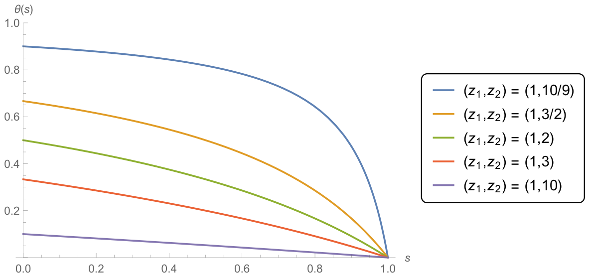
where $t\le z_1<z_2$. With this choice of function, it is easy to show that $\theta \left(s\right)$ is a decreasing, concave down function of s on $[0,t]$. This is indeed verified in Figure 1, which illustrates the behaviour of this function for several $(z_1,z_2)$ pairs in the case when $t=1$. In general, such a choice for $\theta \left(s\right)$ makes practical sense, since you can afford to be more patient and wait for a higher bid to arrive early within the selling window in comparison to later on when the pressure to sell (so that you at least get something for the asset) becomes greater.

In regard to the rate function of the non-homogeneous Poisson process $\left\{N\right(s),s\ge 0\}$, we consider a piecewise constant arrival rate of the following form. Specifically, we let $n\in {\mathbb{Z}}^{+}$ and introduce the sequences ${\left\{{\lambda }_i\right\}}_{i=1}^n$ and ${\left\{t_i\right\}}_{i=0}^n$ such that ${\lambda }_i>0\forall i=1,2,\dots ,n$ and $0=t_0<t_1<\cdots <t_{n-1}<t_n=t$. In other words, ${\lambda }_i$ represents the arrival rate of bids corresponding to the time interval $(t_{i-1},t_i]$.

Under these additional assumptions, (15) gives rise to

$$E\left(R^k\right)={\displaystyle \frac{1}{k+1}}{\displaystyle \sum _{i=1}^n}{\lambda }_i{\int }_{t_{i-1}}^{t_i}\left(1-{\left({\displaystyle \frac{z_1-s}{z_2-s}}\right)}^{k+1}\right)e^{-\left({\sum }_{j=1}^{i-1}{\lambda }_j{\int }_{t_{j-1}}^{t_j}\left(1-{\displaystyle \frac{z_1-v}{z_2-v}}\right)dv+{\lambda }_i{\int }_{t_{i-1}}^s\left(1-{\displaystyle \frac{z_1-v}{z_2-v}}\right)dv\right)}ds.$$

(16)

Note that

$$\begin{array}{ccc}\hfill {\displaystyle \sum _{j=1}^{i-1}}{\lambda }_j{\int }_{t_{j-1}}^{t_j}\left(1-{\displaystyle \frac{z_1-v}{z_2-v}}\right)dv+{\lambda }_i{\int }_{t_{i-1}}^s\left(1-{\displaystyle \frac{z_1-v}{z_2-v}}\right)dv& =& {\displaystyle \sum _{j=1}^{i-1}}{\lambda }_j(z_2-z_1)ln\left({\displaystyle \frac{z_2-t_{j-1}}{z_2-t_j}}\right)+{\lambda }_i(z_2-z_1)ln\left({\displaystyle \frac{z_2-t_{i-1}}{z_2-s}}\right)\hfill \\ & =& {\displaystyle \sum _{j=1}^i}ln{\left({\displaystyle \frac{z_2-t_{j-1}}{z_2-t_j}}\right)}^{{\gamma }_j}+ln{\left({\displaystyle \frac{z_2-t_i}{z_2-s}}\right)}^{{\gamma }_i},\hfill \end{array}$$

(17)

where we define ${\gamma }_i={\lambda }_i(z_2-z_1)$ for $i=1,2,\dots ,n$. Substituting (17) into (16) subsequently leads to

$$E\left(R^k\right)={\displaystyle \frac{1}{k+1}}{\displaystyle \sum _{i=1}^n}{\lambda }_i{\displaystyle \prod _{j=1}^i}{\left({\displaystyle \frac{z_2-t_j}{z_2-t_{j-1}}}\right)}^{{\gamma }_j}{\int }_{t_{i-1}}^{t_i}\left(1-{\left({\displaystyle \frac{z_1-s}{z_2-s}}\right)}^{k+1}\right){\left({\displaystyle \frac{z_2-s}{z_2-t_i}}\right)}^{{\gamma }_i}ds.$$

(18)

Looking at the integral term in (18), we have that

$$\begin{array}{ccc}\hfill & & {\int }_{t_{i-1}}^{t_i}\left(1-{\left({\displaystyle \frac{z_1-s}{z_2-s}}\right)}^{k+1}\right){\left({\displaystyle \frac{z_2-s}{z_2-t_i}}\right)}^{{\gamma }_i}ds\hfill \\ & =& {\int }_{t_{i-1}}^{t_i}{\left({\displaystyle \frac{z_2-s}{z_2-t_i}}\right)}^{{\gamma }_i}ds-{\int }_{t_{i-1}}^{t_i}{\left({\displaystyle \frac{z_1-s}{z_2-t_i}}\right)}^{k+1}{\left({\displaystyle \frac{z_2-s}{z_2-t_i}}\right)}^{{\gamma }_i-k-1}ds\hfill \\ & =& {\displaystyle \frac{z_2-t_i}{{\gamma }_i+1}}\left({\left({\displaystyle \frac{z_2-t_{i-1}}{z_2-t_i}}\right)}^{{\gamma }_i+1}-1\right)-(z_2-t_i){\int }_1^{{\displaystyle \frac{z_2-t_{i-1}}{z_2-t_i}}}{\left(u-{\displaystyle \frac{z_2-z_1}{z_2-t_i}}\right)}^{k+1}{u}^{{\gamma }_i-k-1}du\hfill \\ & =& {\displaystyle \frac{z_2-t_i}{{\gamma }_i+1}}\left({\left({\displaystyle \frac{z_2-t_{i-1}}{z_2-t_i}}\right)}^{{\gamma }_i+1}-1\right)-(z_2-z_1){\displaystyle \sum _{j=0}^{k+1}}\left({\displaystyle \genfrac{}{}{0pt}{}{k+1}{j}}\right){(-1)}^j{\left({\displaystyle \frac{z_2-z_1}{z_2-t_i}}\right)}^{j-1}{\int }_1^{{\displaystyle \frac{z_2-t_{i-1}}{z_2-t_i}}}{u}^{{\gamma }_i-j}du,\hfill \end{array}$$

(19)

where the binomial expansion formula was applied to the term ${\left(u-{\displaystyle \frac{z_2-z_1}{z_2-t_i}}\right)}^{k+1}$. Note that

$$\begin{array}{ccc}\hfill & & {\displaystyle \sum _{j=0}^{k+1}}\left({\displaystyle \genfrac{}{}{0pt}{}{k+1}{j}}\right){(-1)}^j{\left({\displaystyle \frac{z_2-z_1}{z_2-t_i}}\right)}^{j-1}{\int }_1^{{\displaystyle \frac{z_2-t_{i-1}}{z_2-t_i}}}{u}^{{\gamma }_i-j}du\hfill \\ & =& {\displaystyle \frac{z_2-t_i}{z_2-z_1}}{\int }_1^{{\displaystyle \frac{z_2-t_{i-1}}{z_2-t_i}}}{u}^{{\gamma }_i}du-(k+1){\int }_1^{{\displaystyle \frac{z_2-t_{i-1}}{z_2-t_i}}}{u}^{{\gamma }_i-1}du-{\displaystyle \sum _{j=2}^{k+1}}{(-1)}^{j-1}\left({\displaystyle \genfrac{}{}{0pt}{}{k+1}{j}}\right){\left({\displaystyle \frac{z_2-z_1}{z_2-t_i}}\right)}^{j-1}{\int }_1^{{\displaystyle \frac{z_2-t_{i-1}}{z_2-t_i}}}{u}^{{\gamma }_i-j}du\hfill \\ & =& {\displaystyle \frac{z_2-t_i}{(z_2-z_1)({\gamma }_i+1)}}\left({\left({\displaystyle \frac{z_2-t_{i-1}}{z_2-t_i}}\right)}^{{\gamma }_i+1}-1\right)-{\displaystyle \frac{k+1}{{\gamma }_i}}\left({\left({\displaystyle \frac{z_2-t_{i-1}}{z_2-t_i}}\right)}^{{\gamma }_i}-1\right)-{\displaystyle \sum _{\ell =1}^k}{(-1)}^{\ell }\left({\displaystyle \genfrac{}{}{0pt}{}{k+1}{\ell +1}}\right){\left({\displaystyle \frac{z_2-z_1}{z_2-t_i}}\right)}^{\ell }{w}_{i,\ell },\hfill \end{array}$$

(20)

where

$$w_{i,\ell }={\int }_1^{{\displaystyle \frac{z_2-t_{i-1}}{z_2-t_i}}}{u}^{{\gamma }_i-\ell -1}du=\left\{\begin{array}{cc}{\displaystyle \frac{1}{{\gamma }_i-\ell }}\left({\left({\displaystyle \frac{z_2-t_{i-1}}{z_2-t_i}}\right)}^{{\gamma }_i-\ell }-1\right)\hfill & ,\ell \ne {\gamma }_i,\hfill \\ ln\left({\displaystyle \frac{z_2-t_{i-1}}{z_2-t_i}}\right)\hfill & ,\ell ={\gamma }_i.\hfill \end{array}\right.$$

Substituting (20) into (19), we obtain

$$\begin{array}{ccc}& & {\int }_{t_{i-1}}^{t_i}\left(1-{\left({\displaystyle \frac{z_1-s}{z_2-s}}\right)}^{k+1}\right){\left({\displaystyle \frac{z_2-s}{z_2-t_i}}\right)}^{{\gamma }_i}ds\hfill \\ & =& {\displaystyle \frac{(k+1)}{{\lambda }_i}}\left({\left({\displaystyle \frac{z_2-t_{i-1}}{z_2-t_i}}\right)}^{{\gamma }_i}-1\right)+(z_2-z_1){\displaystyle \sum _{\ell =1}^k}{(-1)}^{\ell }\left({\displaystyle \genfrac{}{}{0pt}{}{k+1}{\ell +1}}\right){\left({\displaystyle \frac{z_2-z_1}{z_2-t_i}}\right)}^{\ell }{w}_{i,\ell }.\hfill \end{array}$$

Armed with the above integral result, (18) gives rise to the following final formula for $E\left(R^k\right)$:

$$E\left(R^k\right)=1-{\displaystyle \prod _{j=1}^n}{\left({\displaystyle \frac{z_2-t_j}{z_2-t_{j-1}}}\right)}^{{\gamma }_j}+{\displaystyle \frac{1}{k+1}}{\displaystyle \sum _{i=1}^n}{\gamma }_i{\displaystyle \prod _{j=1}^i}{\left({\displaystyle \frac{z_2-t_j}{z_2-t_{j-1}}}\right)}^{{\gamma }_j}{\displaystyle \sum _{\ell =1}^k}{(-1)}^{\ell }\left({\displaystyle \genfrac{}{}{0pt}{}{k+1}{\ell +1}}\right){\left({\displaystyle \frac{z_2-z_1}{z_2-t_i}}\right)}^{\ell }{w}_{i,\ell }.$$

(21)

To investigate this result numerically, we set $t=1$ and consider several different choices of rate function $\lambda \left(s\right)$ for $0\le s\le 1$. Letting “$RF$” stand for “rate function”, the specific forms of $\lambda \left(s\right)$ we chose to examine were:

$RF1:$

$$\lambda \left(s\right)=1,0\le s\le 1.$$

$RF2:$

$$\lambda \left(s\right)=\left\{\begin{array}{cc}{\displaystyle \frac{5}{4}}\hfill & ,0\le s\le {\displaystyle \frac{1}{2}},\hfill \\ 1\hfill & ,{\displaystyle \frac{1}{2}}<s\le {\displaystyle \frac{3}{4}},\hfill \\ {\displaystyle \frac{1}{2}}\hfill & ,{\displaystyle \frac{3}{4}}<s\le 1.\hfill \end{array}\right.$$

$RF3:$

$$\lambda \left(s\right)=\left\{\begin{array}{cc}{\displaystyle \frac{1}{4}}\hfill & ,0\le s\le {\displaystyle \frac{1}{4}},\hfill \\ {\displaystyle \frac{3}{4}}\hfill & ,{\displaystyle \frac{1}{4}}<s\le {\displaystyle \frac{1}{2}},\hfill \\ 1\hfill & ,{\displaystyle \frac{1}{2}}<s\le {\displaystyle \frac{3}{4}},\hfill \\ 2\hfill & ,{\displaystyle \frac{3}{4}}<s\le 1.\hfill \end{array}\right.$$

$RF4:$

$$\lambda \left(s\right)=\left\{\begin{array}{cc}{\displaystyle \frac{5}{3}}\hfill & ,0\le s\le {\displaystyle \frac{3}{20}},\hfill \\ {\displaystyle \frac{5}{6}}\hfill & ,{\displaystyle \frac{3}{20}}<s\le {\displaystyle \frac{2}{5}},\hfill \\ {\displaystyle \frac{5}{12}}\hfill & ,{\displaystyle \frac{2}{5}}<s\le {\displaystyle \frac{3}{5}},\hfill \\ {\displaystyle \frac{5}{6}}\hfill & ,{\displaystyle \frac{3}{5}}<s\le {\displaystyle \frac{17}{20}},\hfill \\ {\displaystyle \frac{5}{3}}\hfill & ,{\displaystyle \frac{17}{20}}<s\le 1.\hfill \end{array}\right.$$

$RF5:$

$$\lambda \left(s\right)=\left\{\begin{array}{cc}1\hfill & ,0\le s\le {\displaystyle \frac{1}{11}},\hfill \\ {\displaystyle \frac{4}{3}}\hfill & ,{\displaystyle \frac{1}{11}}<s\le {\displaystyle \frac{2}{11}},\hfill \\ {\displaystyle \frac{5}{3}}\hfill & ,{\displaystyle \frac{2}{11}}<s\le {\displaystyle \frac{3}{11}},\hfill \\ 2\hfill & ,{\displaystyle \frac{3}{11}}<s\le {\displaystyle \frac{4}{11}},\hfill \\ {\displaystyle \frac{5}{3}}\hfill & ,{\displaystyle \frac{4}{11}}<s\le {\displaystyle \frac{5}{11}},\hfill \\ {\displaystyle \frac{4}{3}}\hfill & ,{\displaystyle \frac{5}{11}}<s\le {\displaystyle \frac{6}{11}},\hfill \\ {\displaystyle \frac{3}{5}}\hfill & ,{\displaystyle \frac{6}{11}}<s\le {\displaystyle \frac{7}{11}},\hfill \\ {\displaystyle \frac{3}{10}}\hfill & ,{\displaystyle \frac{7}{11}}<s\le {\displaystyle \frac{8}{11}},\hfill \\ {\displaystyle \frac{1}{5}}\hfill & ,{\displaystyle \frac{8}{11}}<s\le {\displaystyle \frac{9}{11}},\hfill \\ {\displaystyle \frac{3}{10}}\hfill & ,{\displaystyle \frac{9}{11}}<s\le {\displaystyle \frac{10}{11}},\hfill \\ {\displaystyle \frac{3}{5}}\hfill & ,{\displaystyle \frac{10}{11}}<s\le 1.\hfill \end{array}\right.$$

It is noteworthy that while all five rate functions yield an expected value of one bid over the interval $[0,1]$, the shapes of these five rate functions are quite varied. If we view $RF$ 1 as a benchmark of sorts (being constant over time, characteristic of a homogeneous Poisson process), then we observe that $RF$ 2 is a non-increasing function, $RF$ 3 is a non-decreasing function, $RF$ 4 is non-monotonic in behaviour, and $RF$ 5 resembles that of a sinusoidal function. For different combinations of $\lambda \left(s\right)$ and threshold amount function $\theta \left(s\right)$ (selected from those depicted in Figure 1),

Table 1. Mean and standardized moments of R for different combinations of rate function and $\theta \left(s\right)=(z_1-s)/(z_2-s)$ for $0\le s\le 1$.

	$({\mathit{z}}_1,{\mathit{z}}_2)=(1,10/9)$	$({\mathit{z}}_1,{\mathit{z}}_2)=(1,3/2)$	$({\mathit{z}}_1,{\mathit{z}}_2)=(1,2)$	$({\mathit{z}}_1,{\mathit{z}}_2)=(1,3)$	$({\mathit{z}}_1,{\mathit{z}}_2)=(1,10)$
$RF1$	$mean=0.1836$	$mean=0.3006$	$mean=0.3267$	$mean=0.3333$	$mean=0.3243$
	$cv=1.9082$	$cv=1.2448$	$cv=1.1037$	$cv=1.0398$	$cv=1.0316$
	$skew=1.4663$	$skew=0.6016$	$skew=0.4470$	$skew=0.4336$	$skew=0.5314$
	$kurt=3.2868$	$kurt=1.6050$	$kurt=1.5659$	$kurt=1.6678$	$kurt=1.8232$
$RF2$	$mean=0.1592$	$mean=0.2905$	$mean=0.3232$	$mean=0.3330$	$mean=0.3248$
	$cv=2.1264$	$cv=1.3011$	$cv=1.1271$	$cv=1.0468$	$cv=1.0306$
	$skew=1.7127$	$skew=0.6580$	$skew=0.4582$	$skew=0.4269$	$skew=0.5272$
	$kurt=4.0338$	$kurt=1.6368$	$kurt=1.5468$	$kurt=1.6492$	$kurt=1.8190$
$RF3$	$mean=0.2304$	$mean=0.3193$	$mean=0.3319$	$mean=0.3320$	$mean=0.3222$
	$cv=1.5952$	$cv=1.1426$	$cv=1.0592$	$cv=1.0286$	$cv=1.0362$
	$skew=1.0783$	$skew=0.4972$	$skew=0.4358$	$skew=0.4606$	$skew=0.5452$
	$kurt=2.3353$	$kurt=1.5763$	$kurt=1.6271$	$kurt=1.7236$	$kurt=1.8374$
$RF4$	$mean=0.1962$	$mean=0.3012$	$mean=0.3261$	$mean=0.3332$	$mean=0.3245$
	$cv=1.7960$	$cv=1.2357$	$cv=1.1052$	$cv=1.0418$	$cv=1.0312$
	$skew=1.3510$	$skew=0.6085$	$skew=0.4567$	$skew=0.4349$	$skew=0.5294$
	$kurt=3.0050$	$kurt=1.6291$	$kurt=1.5723$	$kurt=1.6629$	$kurt=1.8210$
$RF5$	$mean=0.1483$	$mean=0.2837$	$mean=0.3204$	$mean=0.3325$	$mean=0.3250$
	$cv=2.2290$	$cv=1.3379$	$cv=1.1434$	$cv=1.0521$	$cv=1.0304$
	$skew=1.8419$	$skew=0.6995$	$skew=0.4688$	$skew=0.4248$	$skew=0.5256$
	$kurt=4.4967$	$kurt=1.6699$	$kurt=1.5378$	$kurt=1.6397$	$kurt=1.8173$

displays (to 4 decimal places of accuracy) the values of $E\left(R\right)$ as well as the following standardized moments of R:

$$\begin{array}{ccc}\hfill \mathrm{Coefficient}\mathrm{of}\mathrm{Variation}:& & {\displaystyle \frac{E{\left({(R-E\left(R\right))}^2\right)}^{1/2}}{E\left(R\right)}},\hfill \\ \hfill \mathrm{Coefficient}\mathrm{of}\mathrm{Skewness}\text{:}& & {\displaystyle \frac{E\left({(R-E\left(R\right))}^3\right)}{E{\left({(R-E\left(R\right))}^2\right)}^{3/2}}},\hfill \\ \hfill \mathrm{Coefficient}\mathrm{of}\mathrm{Kurtosis}\text{:}& & {\displaystyle \frac{E\left({(R-E\left(R\right))}^4\right)}{E{\left({(R-E\left(R\right))}^2\right)}^2}}.\hfill \end{array}$$

We remark that the central moments $E\left({(R-E\left(R\right))}^k\right)$ and the raw moments $E\left(R^k\right)$ are related via the result (cf. p. 42 in [17])

$$E\left({(R-E\left(R\right))}^k\right)={\displaystyle \sum _{j=0}^k}{(-1)}^j\left({\displaystyle \genfrac{}{}{0pt}{}{k}{j}}\right)E\left(R^{k-j}\right)E{\left(R\right)}^j.$$

The mean and these standardized moments are routinely used in statistical applications to describe the location, variability, skewness, and heavy-tailedness of a probability distribution (cf. Chapter 3 in [18]). In Table 1, these quantities are denoted by “$mean$”, “$cv$”, “$skew$”, and “$kurt$”, respectively.

Table 1 reveals that the distribution of R is positively skewed, particularly for smaller values of $z_2$. In addition, the majority of values of $kurt$ in Table 1 are well below 3, indicative of a thin-tailed distribution for R. For a given choice of rate function, the $cv$ value tends to decrease as $z_2$ increases (the only minor exception occurs when $z_2=10$ for $RF$ 3). On the other hand, if we consider a particular threshold amount function (excluding the $(z_1,z_2)=(1,10/9)$ choice), we observe that the moment-based quantities are fairly robust across all five rate functions. Specifically, the results are very similar across all five rate functions in the case when $(z_1,z_2)=(1,10)$. However, we do recognize that the results are a bit more varied in the case when $(z_1,z_2)=(1,3/2)$, and considerably more so when $(z_1,z_2)=(1,10/9)$. It is also worthwhile to note that regardless of which of the five rate functions is in place, the threshold amount function with $(z_1,z_2)=(1,3)$ always produces the largest $mean$ value. In fact, the value $mean=0.3333$ in the case of $RF$ 1 and $(z_1,z_2)=(1,3)$ agrees with the result found on p. 42 in [16]. This is not too surprising, however, since Katriel [8] has shown that in the case of a homogeneous Poisson process (i.e., $\lambda \left(s\right)=\lambda \forall s$) with bid amounts which are uniformly distributed on $(0,1)$, an explicit expression for the optimal policy to maximize $E\left(R\right)$ is known to be given by (cf. Section 2.3.1 in [8])

$$\theta \left(s\right)={\displaystyle \frac{t-s}{t+2/\lambda -s}},0\le s\le t.$$

In the second example we wish to present, our objective is twofold: to move beyond simply considering uniformly distributed percentage bid amounts (which the first example only dealt with), and to study the effect of a piecewise constant structure on the threshold amount function. For $r\in {\mathbb{Z}}^{+}$, we assume that $\theta \left(s\right)={\theta }_i$ for ${\tau }_{i-1}<s\le {\tau }_i$ where ${\theta }_i\in [0,1]\forall i=1,2,\dots ,r$ and $0={\tau }_0<{\tau }_1<\cdots <{\tau }_{r-1}<{\tau }_r=t$. With this form of $\theta \left(s\right)$, (14) gives rise to

$$\begin{array}{ccc}\hfill E\left(R^k\right)& =& {\displaystyle \frac{{(a+b-1)}_b}{{(a+b+k-1)}_b}}{\displaystyle \sum _{i=1}^r}\overline{B}({\theta }_i;a+k,b){\int }_{{\tau }_{i-1}}^{{\tau }_i}\lambda \left(s\right)e^{-\left({\sum }_{j=1}^{i-1}\overline{B}({\theta }_j;a,b){\int }_{{\tau }_{j-1}}^{{\tau }_j}\lambda \left(v\right)dv+\overline{B}({\theta }_i;a,b){\int }_{{\tau }_{i-1}}^s\lambda \left(v\right)dv\right)}ds\hfill \\ & =& {\displaystyle \frac{{(a+b-1)}_b}{{(a+b+k-1)}_b}}{\displaystyle \sum _{i=1}^r}{\displaystyle \frac{\overline{B}({\theta }_i;a+k,b)}{\overline{B}({\theta }_i;a,b)}}{e}^{-{\sum }_{j=1}^{i-1}\overline{B}({\theta }_j;a,b)\left(m\left({\tau }_j\right)-m\left({\tau }_{j-1}\right)\right)}{\int }_0^{m\left({\tau }_i\right)-m\left({\tau }_{i-1}\right)}\overline{B}({\theta }_i;a,b)e^{-\overline{B}({\theta }_i;a,b)u}du\hfill \\ & =& {\displaystyle \frac{{(a+b-1)}_b}{{(a+b+k-1)}_b}}{\displaystyle \sum _{i=1}^r}{\displaystyle \frac{\overline{B}({\theta }_i;a+k,b)}{\overline{B}({\theta }_i;a,b)}}\left(e^{-{\sum }_{j=1}^{i-1}\overline{B}({\theta }_j;a,b)\left(m\left({\tau }_j\right)-m\left({\tau }_{j-1}\right)\right)}-e^{-{\sum }_{j=1}^i\overline{B}({\theta }_j;a,b)\left(m\left({\tau }_j\right)-m\left({\tau }_{j-1}\right)\right)}\right).\hfill \end{array}$$

(22)

In the case when $r=1$ (which we will refer to as model “$TAF$ 1”), (22) reduces to

$$E\left(R^k\right)={\displaystyle \frac{{(a+b-1)}_b}{{(a+b+k-1)}_b}}{\displaystyle \frac{\overline{B}({\theta }_1;a+k,b)}{\overline{B}({\theta }_1;a,b)}}\left(1-e^{-\overline{B}({\theta }_1;a,b)m\left(t\right)}\right).$$

(23)

An interesting observation regarding (23) is that if ${\lambda }_1\left(s\right)$ and ${\lambda }_2\left(s\right)$ are two distinct rate functions such that ${\int }_0^t{\lambda }_1\left(s\right)ds={\int }_0^t{\lambda }_2\left(s\right)ds$, then the values of $E\left(R^k\right)$ for either rate function will be identical. In other words, the raw moments of R are independent of the actual form of rate function in place and depend only on the value of the quantity $m\left(t\right)$.

As a practical application involving $TAF$ 1, suppose that $t=1$, $m\left(1\right)=5$, and $k=1$.

Table 2. Optimal values of $E\left(R\right)$ and ${\theta }_1$ under $TAF$ 1 for any rate function $\lambda \left(s\right)$ with $m\left(1\right)=5$.

	$b=1$	$b=2$	$b=3$	$b=4$	$b=5$
$a=1$	$E{\left(R\right)}^{*}=0.6936$	$E{\left(R\right)}^{*}=0.5010$	$E{\left(R\right)}^{*}=0.3895$	$E{\left(R\right)}^{*}=0.3181$	$E{\left(R\right)}^{*}=0.2686$
	${\theta }_1^{*}=0.5645$	${\theta }_1^{*}=0.3899$	${\theta }_1^{*}=0.2972$	${\theta }_1^{*}=0.2400$	${\theta }_1^{*}=0.2012$
$a=2$	$E{\left(R\right)}^{*}=0.7923$	$E{\left(R\right)}^{*}=0.6322$	$E{\left(R\right)}^{*}=0.5226$	$E{\left(R\right)}^{*}=0.4445$	$E{\left(R\right)}^{*}=0.3864$
	${\theta }_1^{*}=0.6823$	${\theta }_1^{*}=0.5239$	${\theta }_1^{*}=0.4247$	${\theta }_1^{*}=0.3569$	${\theta }_1^{*}=0.3077$
$a=3$	$E{\left(R\right)}^{*}=0.8377$	$E{\left(R\right)}^{*}=0.7031$	$E{\left(R\right)}^{*}=0.6025$	$E{\left(R\right)}^{*}=0.5261$	$E{\left(R\right)}^{*}=0.4664$
	${\theta }_1^{*}=0.7410$	${\theta }_1^{*}=0.6017$	${\theta }_1^{*}=0.5063$	${\theta }_1^{*}=0.4369$	${\theta }_1^{*}=0.3843$
$a=4$	$E{\left(R\right)}^{*}=0.8647$	$E{\left(R\right)}^{*}=0.7487$	$E{\left(R\right)}^{*}=0.6571$	$E{\left(R\right)}^{*}=0.5845$	$E{\left(R\right)}^{*}=0.5259$
	${\theta }_1^{*}=0.7774$	${\theta }_1^{*}=0.6539$	${\theta }_1^{*}=0.5644$	${\theta }_1^{*}=0.4965$	${\theta }_1^{*}=0.4431$
$a=5$	$E{\left(R\right)}^{*}=0.8829$	$E{\left(R\right)}^{*}=0.7808$	$E{\left(R\right)}^{*}=0.6972$	$E{\left(R\right)}^{*}=0.6289$	$E{\left(R\right)}^{*}=0.5723$
	${\theta }_1^{*}=0.8027$	${\theta }_1^{*}=0.6918$	${\theta }_1^{*}=0.6083$	${\theta }_1^{*}=0.5429$	${\theta }_1^{*}=0.4902$

displays (to 4 decimal places of accuracy) the values of ${\theta }_1$ which maximize $E\left(R\right)$ under a variety of beta-distributed percentage bid amounts. The optimal values of ${\theta }_1$ and $E\left(R\right)$ are denoted with asterisks in Table 2. We point out that values of ${\theta }_1^{*}$ were obtained by differentiating (23) with $k=1$, setting the resulting expression equal to 0, and numerically solving for the corresponding roots. Looking at the results in Table 2, we observe that the values of ${\theta }_1^{*}$ decrease as one moves from left to right across a given row of the table. This makes intuitive sense since, for a given value of a, the mean of the percentage bid amount random variable decreases as b increases. Since it is less likely that a “high” bid will be received, we should lower our expectations accordingly by choosing a lower threshold amount. On the other hand, the values of ${\theta }_1^{*}$ increase as one moves from top to bottom across a given column of Table 2. In this situation, for a fixed value of b, the mean of the percentage bid amount random variable increases as a increases. On the main diagonal of Table 2 when $a=b$, the percentage bid amounts all have a mean of $1/2$ but their variances decrease as a and b get larger, and this results in gradually lower values of ${\theta }_1^{*}$ and $E{\left(R\right)}^{*}$.

As a means of comparison, let us consider the same optimization problem but in the case when $r=2$ (which we will refer to as model “$TAF$ 2”). When $r=2$ and $k=1$, (22) simplifies to become

$$E\left(R\right)={\displaystyle \frac{a}{a+b}}\left({\displaystyle \frac{\overline{B}({\theta }_1;a+1,b)}{\overline{B}({\theta }_1;a,b)}}\left(1-e^{-\overline{B}({\theta }_1;a,b)m\left({\tau }_1\right)}\right)+{\displaystyle \frac{\overline{B}({\theta }_2;a+1,b)}{\overline{B}({\theta }_2;a,b)}}{e}^{-\overline{B}({\theta }_1;a,b)m\left({\tau }_1\right)}\left(1-e^{-\overline{B}({\theta }_2;a,b)\left(m\left(t\right)-m\left({\tau }_1\right)\right)}\right)\right).$$

(24)

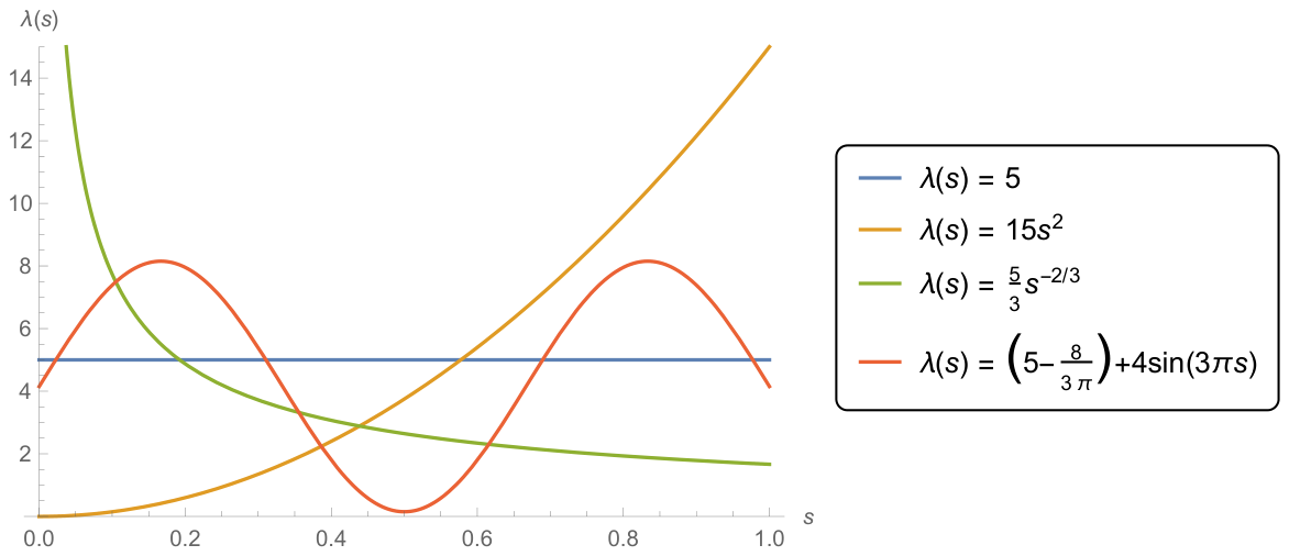
For $t=1$ and a given pair of $(a,b)$ values, our goal is to maximize $E\left(R\right)$ with respect to the three variables ${\theta }_1$, ${\theta }_2$, and ${\tau }_1$. Unlike the situation when $r=1$, however, the presence of ${\tau }_1$ in (24) suggests that the form of the rate function $\lambda \left(s\right)$ now plays a role. To that point, let us consider the four different rate functions depicted in Figure 2. There is clear variation in the shapes of these four rate functions, but it is readily verified that $m\left(1\right)=5$ for each of them. As such, this will make the comparison more pertinent with $TAF$ 1.

Table 3. Optimal values of $E\left(R\right)$, ${\theta }_1$, ${\theta }_2$, and ${\tau }_1$ for different rate functions under $TAF$ 2.

	Rate Function $\lambda \left(s\right)=5$ for $0\le s\le 1$
	$b=1$	$b=2$	$b=3$	$b=4$	$b=5$
$a=1$	$E{\left(R\right)}^{*}=0.7083$	$E{\left(R\right)}^{*}=0.5142$	$E{\left(R\right)}^{*}=0.4005$	$E{\left(R\right)}^{*}=0.3274$	$E{\left(R\right)}^{*}=0.2766$
	$({\theta }_1^{*},{\theta }_2^{*})=(0.6381,0.3492)$	$({\theta }_1^{*},{\theta }_2^{*})=(0.4507,0.2283)$	$({\theta }_1^{*},{\theta }_2^{*})=(0.3468,0.1698)$	$({\theta }_1^{*},{\theta }_2^{*})=(0.2814,0.1352)$	$({\theta }_1^{*},{\theta }_2^{*})=(0.2367,0.1123)$
	${\tau }_1^{*}=0.5956$	${\tau }_1^{*}=0.6106$	${\tau }_1^{*}=0.6168$	${\tau }_1^{*}=0.6203$	${\tau }_1^{*}=0.6224$
$a=2$	$E{\left(R\right)}^{*}=0.8069$	$E{\left(R\right)}^{*}=0.6476$	$E{\left(R\right)}^{*}=0.5368$	$E{\left(R\right)}^{*}=0.4573$	$E{\left(R\right)}^{*}=0.3978$
	$({\theta }_1^{*},{\theta }_2^{*})=(0.7506,0.4667)$	$({\theta }_1^{*},{\theta }_2^{*})=(0.5887,0.3401)$	$({\theta }_1^{*},{\theta }_2^{*})=(0.4821,0.2684)$	$({\theta }_1^{*},{\theta }_2^{*})=(0.4076,0.2219)$	$({\theta }_1^{*},{\theta }_2^{*})=(0.3528,0.1892)$
	${\tau }_1^{*}=0.5762$	${\tau }_1^{*}=0.5955$	${\tau }_1^{*}=0.6043$	${\tau }_1^{*}=0.6094$	${\tau }_1^{*}=0.6127$
$a=3$	$E{\left(R\right)}^{*}=0.8512$	$E{\left(R\right)}^{*}=0.7186$	$E{\left(R\right)}^{*}=0.6176$	$E{\left(R\right)}^{*}=0.5403$	$E{\left(R\right)}^{*}=0.4796$
	$({\theta }_1^{*},{\theta }_2^{*})=(0.8039,0.5354)$	$({\theta }_1^{*},{\theta }_2^{*})=(0.6656,0.4145)$	$({\theta }_1^{*},{\theta }_2^{*})=(0.5658,0.3397)$	$({\theta }_1^{*},{\theta }_2^{*})=(0.4913,0.2882)$	$({\theta }_1^{*},{\theta }_2^{*})=(0.4339,0.2505)$
	${\tau }_1^{*}=0.5592$	${\tau }_1^{*}=0.5812$	${\tau }_1^{*}=0.5917$	${\tau }_1^{*}=0.5981$	${\tau }_1^{*}=0.6023$
$a=4$	$E{\left(R\right)}^{*}=0.8770$	$E{\left(R\right)}^{*}=0.7637$	$E{\left(R\right)}^{*}=0.6724$	$E{\left(R\right)}^{*}=0.5992$	$E{\left(R\right)}^{*}=0.5399$
	$({\theta }_1^{*},{\theta }_2^{*})=(0.8359,0.5824)$	$({\theta }_1^{*},{\theta }_2^{*})=(0.7158,0.4690)$	$({\theta }_1^{*},{\theta }_2^{*})=(0.6238,0.3947)$	$({\theta }_1^{*},{\theta }_2^{*})=(0.5522,0.3414)$	$({\theta }_1^{*},{\theta }_2^{*})=(0.4950,0.3010)$
	${\tau }_1^{*}=0.5440$	${\tau }_1^{*}=0.5679$	${\tau }_1^{*}=0.5799$	${\tau }_1^{*}=0.5872$	${\tau }_1^{*}=0.5922$
$a=5$	$E{\left(R\right)}^{*}=0.8942$	$E{\left(R\right)}^{*}=0.7952$	$E{\left(R\right)}^{*}=0.7122$	$E{\left(R\right)}^{*}=0.6437$	$E{\left(R\right)}^{*}=0.5866$
	$({\theta }_1^{*},{\theta }_2^{*})=(0.8577,0.6175)$	$({\theta }_1^{*},{\theta }_2^{*})=(0.7515,0.5114)$	$({\theta }_1^{*},{\theta }_2^{*})=(0.6669,0.4389)$	$({\theta }_1^{*},{\theta }_2^{*})=(0.5989,0.3853)$	$({\theta }_1^{*},{\theta }_2^{*})=(0.5432,0.3437)$
	${\tau }_1^{*}=0.5304$	${\tau }_1^{*}=0.5557$	${\tau }_1^{*}=0.5688$	${\tau }_1^{*}=0.5770$	${\tau }_1^{*}=0.5826$
	Rate Function $\lambda \left(s\right)=15s^2$ for $0\le s\le 1$
	$b=1$	$b=2$	$b=3$	$b=4$	$b=5$
$a=1$	$E{\left(R\right)}^{*}=0.7083$	$E{\left(R\right)}^{*}=0.5142$	$E{\left(R\right)}^{*}=0.4005$	$E{\left(R\right)}^{*}=0.3274$	$E{\left(R\right)}^{*}=0.2766$
	$({\theta }_1^{*},{\theta }_2^{*})=(0.6381,0.3492)$	$({\theta }_1^{*},{\theta }_2^{*})=(0.4507,0.2283)$	$({\theta }_1^{*},{\theta }_2^{*})=(0.3468,0.1698)$	$({\theta }_1^{*},{\theta }_2^{*})=(0.2814,0.1352)$	$({\theta }_1^{*},{\theta }_2^{*})=(0.2367,0.1123)$
	${\tau }_1^{*}=0.8414$	${\tau }_1^{*}=0.8484$	${\tau }_1^{*}=0.8512$	${\tau }_1^{*}=0.8528$	${\tau }_1^{*}=0.8538$
$a=2$	$E{\left(R\right)}^{*}=0.8069$	$E{\left(R\right)}^{*}=0.6476$	$E{\left(R\right)}^{*}=0.5368$	$E{\left(R\right)}^{*}=0.4573$	$E{\left(R\right)}^{*}=0.3978$
	$({\theta }_1^{*},{\theta }_2^{*})=(0.7506,0.4667)$	$({\theta }_1^{*},{\theta }_2^{*})=(0.5887,0.3401)$	$({\theta }_1^{*},{\theta }_2^{*})=(0.4821,0.2684)$	$({\theta }_1^{*},{\theta }_2^{*})=(0.4076,0.2219)$	$({\theta }_1^{*},{\theta }_2^{*})=(0.3528,0.1892)$
	${\tau }_1^{*}=0.8322$	${\tau }_1^{*}=0.8413$	${\tau }_1^{*}=0.8454$	${\tau }_1^{*}=0.8478$	${\tau }_1^{*}=0.8493$
$a=3$	$E{\left(R\right)}^{*}=0.8512$	$E{\left(R\right)}^{*}=0.7186$	$E{\left(R\right)}^{*}=0.6176$	$E{\left(R\right)}^{*}=0.5403$	$E{\left(R\right)}^{*}=0.4796$
	$({\theta }_1^{*},{\theta }_2^{*})=(0.8039,0.5354)$	$({\theta }_1^{*},{\theta }_2^{*})=(0.6656,0.4145)$	$({\theta }_1^{*},{\theta }_2^{*})=(0.5658,0.3397)$	$({\theta }_1^{*},{\theta }_2^{*})=(0.4913,0.2882)$	$({\theta }_1^{*},{\theta }_2^{*})=(0.4339,0.2505)$
	${\tau }_1^{*}=0.8239$	${\tau }_1^{*}=0.8345$	${\tau }_1^{*}=0.8395$	${\tau }_1^{*}=0.8425$	${\tau }_1^{*}=0.8445$
$a=4$	$E{\left(R\right)}^{*}=0.8770$	$E{\left(R\right)}^{*}=0.7637$	$E{\left(R\right)}^{*}=0.6724$	$E{\left(R\right)}^{*}=0.5992$	$E{\left(R\right)}^{*}=0.5399$
	$({\theta }_1^{*},{\theta }_2^{*})=(0.8359,0.5824)$	$({\theta }_1^{*},{\theta }_2^{*})=(0.7158,0.4690)$	$({\theta }_1^{*},{\theta }_2^{*})=(0.6238,0.3947)$	$({\theta }_1^{*},{\theta }_2^{*})=(0.5522,0.3414)$	$({\theta }_1^{*},{\theta }_2^{*})=(0.4950,0.3010)$
	${\tau }_1^{*}=0.8164$	${\tau }_1^{*}=0.8281$	${\tau }_1^{*}=0.8339$	${\tau }_1^{*}=0.8374$	${\tau }_1^{*}=0.8398$
$a=5$	$E{\left(R\right)}^{*}=0.8942$	$E{\left(R\right)}^{*}=0.7952$	$E{\left(R\right)}^{*}=0.7122$	$E{\left(R\right)}^{*}=0.6437$	$E{\left(R\right)}^{*}=0.5866$
	$({\theta }_1^{*},{\theta }_2^{*})=(0.8577,0.6175)$	$({\theta }_1^{*},{\theta }_2^{*})=(0.7515,0.5114)$	$({\theta }_1^{*},{\theta }_2^{*})=(0.6669,0.4389)$	$({\theta }_1^{*},{\theta }_2^{*})=(0.5989,0.3853)$	$({\theta }_1^{*},{\theta }_2^{*})=(0.5432,0.3437)$
	${\tau }_1^{*}=0.8095$	${\tau }_1^{*}=0.8222$	${\tau }_1^{*}=0.8286$	${\tau }_1^{*}=0.8325$	${\tau }_1^{*}=0.8352$
	Rate Function $\lambda \left(s\right)={\displaystyle \frac{5}{3}}{s}^{-2/3}$ for $0\le s\le 1$
	$b=1$	$b=2$	$b=3$	$b=4$	$b=5$
$a=1$	$E{\left(R\right)}^{*}=0.7083$	$E{\left(R\right)}^{*}=0.5142$	$E{\left(R\right)}^{*}=0.4005$	$E{\left(R\right)}^{*}=0.3274$	$E{\left(R\right)}^{*}=0.2766$
	$({\theta }_1^{*},{\theta }_2^{*})=(0.6381,0.3492)$	$({\theta }_1^{*},{\theta }_2^{*})=(0.4507,0.2283)$	$({\theta }_1^{*},{\theta }_2^{*})=(0.3468,0.1698)$	$({\theta }_1^{*},{\theta }_2^{*})=(0.2814,0.1352)$	$({\theta }_1^{*},{\theta }_2^{*})=(0.2367,0.1123)$
	${\tau }_1^{*}=0.2113$	${\tau }_1^{*}=0.2276$	${\tau }_1^{*}=0.2347$	${\tau }_1^{*}=0.2386$	${\tau }_1^{*}=0.2412$
$a=2$	$E{\left(R\right)}^{*}=0.8069$	$E{\left(R\right)}^{*}=0.6476$	$E{\left(R\right)}^{*}=0.5368$	$E{\left(R\right)}^{*}=0.4573$	$E{\left(R\right)}^{*}=0.3978$
	$({\theta }_1^{*},{\theta }_2^{*})=(0.7506,0.4667)$	$({\theta }_1^{*},{\theta }_2^{*})=(0.5887,0.3401)$	$({\theta }_1^{*},{\theta }_2^{*})=(0.4821,0.2684)$	$({\theta }_1^{*},{\theta }_2^{*})=(0.4076,0.2219)$	$({\theta }_1^{*},{\theta }_2^{*})=(0.3528,0.1892)$
	${\tau }_1^{*}=0.1913$	${\tau }_1^{*}=0.2112$	${\tau }_1^{*}=0.2207$	${\tau }_1^{*}=0.2263$	${\tau }_1^{*}=0.2300$
$a=3$	$E{\left(R\right)}^{*}=0.8512$	$E{\left(R\right)}^{*}=0.7186$	$E{\left(R\right)}^{*}=0.6176$	$E{\left(R\right)}^{*}=0.5403$	$E{\left(R\right)}^{*}=0.4796$
	$({\theta }_1^{*},{\theta }_2^{*})=(0.8039,0.5354)$	$({\theta }_1^{*},{\theta }_2^{*})=(0.6656,0.4145)$	$({\theta }_1^{*},{\theta }_2^{*})=(0.5658,0.3397)$	$({\theta }_1^{*},{\theta }_2^{*})=(0.4913,0.2882)$	$({\theta }_1^{*},{\theta }_2^{*})=(0.4339,0.2505)$
	${\tau }_1^{*}=0.1749$	${\tau }_1^{*}=0.1963$	${\tau }_1^{*}=0.2072$	${\tau }_1^{*}=0.2139$	${\tau }_1^{*}=0.2185$
$a=4$	$E{\left(R\right)}^{*}=0.8770$	$E{\left(R\right)}^{*}=0.7637$	$E{\left(R\right)}^{*}=0.6724$	$E{\left(R\right)}^{*}=0.5992$	$E{\left(R\right)}^{*}=0.5399$
	$({\theta }_1^{*},{\theta }_2^{*})=(0.8359,0.5824)$	$({\theta }_1^{*},{\theta }_2^{*})=(0.7158,0.4690)$	$({\theta }_1^{*},{\theta }_2^{*})=(0.6238,0.3947)$	$({\theta }_1^{*},{\theta }_2^{*})=(0.5522,0.3414)$	$({\theta }_1^{*},{\theta }_2^{*})=(0.4950,0.3010)$
	${\tau }_1^{*}=0.1610$	${\tau }_1^{*}=0.1832$	${\tau }_1^{*}=0.1950$	${\tau }_1^{*}=0.2025$	${\tau }_1^{*}=0.2077$
$a=5$	$E{\left(R\right)}^{*}=0.8942$	$E{\left(R\right)}^{*}=0.7952$	$E{\left(R\right)}^{*}=0.7122$	$E{\left(R\right)}^{*}=0.6437$	$E{\left(R\right)}^{*}=0.5866$
	$({\theta }_1^{*},{\theta }_2^{*})=(0.8577,0.6175)$	$({\theta }_1^{*},{\theta }_2^{*})=(0.7515,0.5114)$	$({\theta }_1^{*},{\theta }_2^{*})=(0.6669,0.4389)$	$({\theta }_1^{*},{\theta }_2^{*})=(0.5989,0.3853)$	$({\theta }_1^{*},{\theta }_2^{*})=(0.5432,0.3437)$
	${\tau }_1^{*}=0.1492$	${\tau }_1^{*}=0.1716$	${\tau }_1^{*}=0.1840$	${\tau }_1^{*}=0.1921$	${\tau }_1^{*}=0.1978$
	Rate Function $\lambda \left(s\right)=\left(5-\frac{8}{3\pi }\right)+4sin\left(3\pi s\right)$ for $0\le s\le 1$
	$b=1$	$b=2$	$b=3$	$b=4$	$b=5$
$a=1$	$E{\left(R\right)}^{*}=0.7083$	$E{\left(R\right)}^{*}=0.5142$	$E{\left(R\right)}^{*}=0.4005$	$E{\left(R\right)}^{*}=0.3274$	$E{\left(R\right)}^{*}=0.2766$
	$({\theta }_1^{*},{\theta }_2^{*})=(0.6381,0.3492)$	$({\theta }_1^{*},{\theta }_2^{*})=(0.4507,0.2283)$	$({\theta }_1^{*},{\theta }_2^{*})=(0.3468,0.1698)$	$({\theta }_1^{*},{\theta }_2^{*})=(0.2814,0.1352)$	$({\theta }_1^{*},{\theta }_2^{*})=(0.2367,0.1123)$
	${\tau }_1^{*}=0.7093$	${\tau }_1^{*}=0.7219$	${\tau }_1^{*}=0.7269$	${\tau }_1^{*}=0.7296$	${\tau }_1^{*}=0.7313$
$a=2$	$E{\left(R\right)}^{*}=0.8069$	$E{\left(R\right)}^{*}=0.6476$	$E{\left(R\right)}^{*}=0.5368$	$E{\left(R\right)}^{*}=0.4573$	$E{\left(R\right)}^{*}=0.3978$
	$({\theta }_1^{*},{\theta }_2^{*})=(0.7506,0.4667)$	$({\theta }_1^{*},{\theta }_2^{*})=(0.5887,0.3401)$	$({\theta }_1^{*},{\theta }_2^{*})=(0.4821,0.2684)$	$({\theta }_1^{*},{\theta }_2^{*})=(0.4076,0.2219)$	$({\theta }_1^{*},{\theta }_2^{*})=(0.3528,0.1892)$
	${\tau }_1^{*}=0.6913$	${\tau }_1^{*}=0.7092$	${\tau }_1^{*}=0.7167$	${\tau }_1^{*}=0.7209$	${\tau }_1^{*}=0.7236$
$a=3$	$E{\left(R\right)}^{*}=0.8512$	$E{\left(R\right)}^{*}=0.7186$	$E{\left(R\right)}^{*}=0.6176$	$E{\left(R\right)}^{*}=0.5403$	$E{\left(R\right)}^{*}=0.4796$
	$({\theta }_1^{*},{\theta }_2^{*})=(0.8039,0.5354)$	$({\theta }_1^{*},{\theta }_2^{*})=(0.6656,0.4145)$	$({\theta }_1^{*},{\theta }_2^{*})=(0.5658,0.3397)$	$({\theta }_1^{*},{\theta }_2^{*})=(0.4913,0.2882)$	$({\theta }_1^{*},{\theta }_2^{*})=(0.4339,0.2505)$
	${\tau }_1^{*}=0.6733$	${\tau }_1^{*}=0.6961$	${\tau }_1^{*}=0.7059$	${\tau }_1^{*}=0.7114$	${\tau }_1^{*}=0.7150$
$a=4$	$E{\left(R\right)}^{*}=0.8770$	$E{\left(R\right)}^{*}=0.7637$	$E{\left(R\right)}^{*}=0.6724$	$E{\left(R\right)}^{*}=0.5992$	$E{\left(R\right)}^{*}=0.5399$
	$({\theta }_1^{*},{\theta }_2^{*})=(0.8359,0.5824)$	$({\theta }_1^{*},{\theta }_2^{*})=(0.7158,0.4690)$	$({\theta }_1^{*},{\theta }_2^{*})=(0.6238,0.3947)$	$({\theta }_1^{*},{\theta }_2^{*})=(0.5522,0.3414)$	$({\theta }_1^{*},{\theta }_2^{*})=(0.4950,0.3010)$
	${\tau }_1^{*}=0.6546$	${\tau }_1^{*}=0.6829$	${\tau }_1^{*}=0.6949$	${\tau }_1^{*}=0.7018$	${\tau }_1^{*}=0.7063$
$a=5$	$E{\left(R\right)}^{*}=0.8942$	$E{\left(R\right)}^{*}=0.7952$	$E{\left(R\right)}^{*}=0.7122$	$E{\left(R\right)}^{*}=0.6437$	$E{\left(R\right)}^{*}=0.5866$
	$({\theta }_1^{*},{\theta }_2^{*})=(0.8577,0.6175)$	$({\theta }_1^{*},{\theta }_2^{*})=(0.7515,0.5114)$	$({\theta }_1^{*},{\theta }_2^{*})=(0.6669,0.4389)$	$({\theta }_1^{*},{\theta }_2^{*})=(0.5989,0.3853)$	$({\theta }_1^{*},{\theta }_2^{*})=(0.5432,0.3437)$
	${\tau }_1^{*}=0.6341$	${\tau }_1^{*}=0.6693$	${\tau }_1^{*}=0.6838$	${\tau }_1^{*}=0.6921$	${\tau }_1^{*}=0.6975$

displays (to 4 decimal places of accuracy) the values of ${\theta }_1$, ${\theta }_2$, and ${\tau }_1$ which maximize $E\left(R\right)$ under a variety of beta-distributed percentage bid amounts corresponding to each of the four rate functions shown in Figure 2. Analogous to how Table 2 was compiled, we computed the optimal values ${\theta }_1^{*}$, ${\theta }_2^{*}$, and ${\tau }_1^{*}$ by taking partial derivatives of (24), setting the resulting expressions equal to 0, and simultaneously solving for the critical points. Using the Wolfram Mathematica 11.1 software package, we employed the built-in command “NSolve” to carry out this procedure. The same kinds of trends we observed in Table 2 are once again on display in Table 3. As expected, with a more general model featuring the inclusion of more variables, the optimal values of $E\left(R\right)$ in Table 3 are larger than their $TAF$ 1 counterparts in Table 2. However, the increase is fairly modest, amounting to about a 2% increase across all pairs of $(a,b)$ values.

What is perhaps more surprising to observe from Table 3 is that regardless of which rate function is in use, the values of ${\theta }_1^{*}$, ${\theta }_2^{*}$, and $E{\left(R\right)}^{*}$ remain unchanged for a given $(a,b)$ pair. Moreover, any value of ${\theta }_1^{*}$ from Table 2 lies within the interval formed by ${\theta }_1^{*}$ and ${\theta }_2^{*}$ taken from its corresponding entry in Table 3. What does change though, depending on the rate function in place, is the optimal value of ${\tau }_1$. For instance, when there is a greater chance of observing more bids later in the time interval (as in the case when $\lambda \left(s\right)=15s^2$), the value of ${\tau }_1^{*}$ is notably larger and closer to 1. In stark contrast, when it is likelier to observe more bids earlier in the time interval (as in the case when $\lambda \left(s\right)=(5/3)s^{-2/3}$), the value of ${\tau }_1^{*}$ is markedly smaller and closer to 0.

References

1. Karlin, S. Stochastic models and optimal policy for selling an asset. In Studies in Applied Probability and Management Science; Arrow, K.J., Karlin, S., Scarf, H.E., Eds.; Stanford University Press: Stanford, CA, USA, 1962; pp. 148–158. [Google Scholar]
2. Karlin, S.; Taylor, H.M. An Introduction to Stochastic Modeling, 3rd ed.; Academic Press: San Diego, CA, USA, 1998. [Google Scholar]
3. Elfving, G. A persistency problem connected with a point process. J. Appl. Probab. 1967, 4, 77–89. [Google Scholar] [CrossRef] [Scilit]
4. Sakaguchi, M. Optimal stopping problems for randomly arriving offers. Math. Jpn. 1976, 21, 201–217. [Google Scholar]
5. David, I.; Yechiali, U. A time-dependent stopping problem with application to live organ transplants. Oper. Res. 1976, 33, 491–504. [Google Scholar]
6. Stadje, W. An optimal k-stopping problem for the Poisson process. In Mathematical Statistics and Probability Theory, Volume B; Bauer, P., Konecny, F., Wertz, W., Eds.; Springer: Dordrecht, The Netherlands, 1987; pp. 231–244. [Google Scholar]
7. Allaart, P.C. Prophet inequalities for i.i.d. random variables with random arrival times. Seq. Anal. 2007, 26, 403–413. [Google Scholar] [CrossRef] [Scilit]
8. Katriel, G. The Cayley-Moser problem with Poissonian arrival of offers. arXiv 2025, arXiv:2511.02763. [Google Scholar]
9. Bluhm, C.; Overbeck, L.; Wagner, C. Introduction to Credit Risk Modeling, 2nd ed.; Chapman & Hall/CRC: Boca Raton, FL, USA, 2010. [Google Scholar]
10. Modarres, M.; Kaminskiy, M.; Krivtsov, V. Reliability Engineering and Risk Analysis: A Practical Guide; Marcel Dekker Inc.: New York, NY, USA, 1999. [Google Scholar]
11. Ross, S.M. Stochastic Processes, 2nd ed.; John Wiley & Sons: New York, NY, USA, 1996. [Google Scholar]
12. David, H.A.; Nagaraja, H.N. Order Statistics, 3rd ed.; John Wiley & Sons: New York, NY, USA, 2003. [Google Scholar]
13. Ross, S.M. A First Course in Probability, 7th ed.; Pearson Prentice Hall: Upper Saddle River, NJ, USA, 2006. [Google Scholar]
14. Johnson, N.L.; Kotz, S.; Balakrishnan, N. Continuous Univariate Distributions, 2nd ed.; John Wiley & Sons: New York, NY, USA, 1995; Volume 2. [Google Scholar]
15. Spivey, M.Z. The Art of Proving Binomial Identities; Chapman & Hall/CRC: Boca Raton, FL, USA, 2019. [Google Scholar]
16. Karlin, S.; Taylor, H.M. Solutions to Problems in an Introduction to Stochastic Modeling, 3rd ed.; Academic Press: San Diego, CA, USA, 1998. [Google Scholar]
17. Johnson, N.L.; Kotz, S.; Kemp, A.W. Univariate Discrete Distributions, 2nd ed.; John Wiley & Sons: New York, NY, USA, 1992. [Google Scholar]
18. Stuart, A.; Ord, J.K. Kendall’s Advanced Theory of Statistics, Volume 1: Distribution Theory, 6th ed.; John Wiley & Sons: New York, NY, USA, 2010. [Google Scholar]
Figure 1. Plots of θ ( s ) = ( z 1 s ) / ( z 2 s ) for t = 1 and several combinations of z 1 and z 2 .
Mathematics 14 02712 g001
Figure 2. Rate functions for investigation under T A F 2.
Mathematics 14 02712 g002