Closed-Form Covariance Matrix for Portfolio Optimization: Theory and Empirical Evidence Under a Multidimensional Black–Scholes Model with Time-Varying Parameters

Abstract

This paper develops a model-driven analytical framework for portfolio optimization under a multidimensional Black–Scholes model with time-varying parameters, where both the drift and volatility functions evolve linearly over time. Within this framework, explicit closed-form expressions are derived for the covariance matrix of normalized asset prices and subsequently incorporated into the classical Markowitz mean–variance framework to obtain analytical representations of the global minimum-variance portfolio, the mean–variance efficient portfolio, and the corresponding efficient frontier. The proposed methodology establishes a direct connection between continuous-time stochastic asset-price modeling and portfolio optimization through a model-implied covariance structure. Its practical implementation is investigated through both numerical experiments and an empirical study using daily stock price data from 20 constituents of the $S\&P$ 500 index over the period 2020–2024. Monte Carlo simulations demonstrate the finite-sample sensitivity of portfolio optimization to covariance estimation, while the empirical analysis illustrates how the estimated model parameters, obtained using the maximum likelihood framework of Aït-Sahalia for discretely sampled diffusion processes, can be incorporated into the analytical covariance matrix for constructing efficient frontiers under realistic market conditions. Overall, the proposed framework provides an analytically tractable methodology that integrates continuous-time asset pricing models with classical mean–variance portfolio optimization, offering a coherent model-based covariance representation for portfolio selection under time-varying market environments.

1. Introduction

Covariance matrix estimation is a fundamental problem in statistics and quantitative finance, as it characterizes the dependence structure among asset returns and plays a central role in risk analysis and portfolio optimization. Markowitz’s Modern Portfolio Theory (MPT) [1,2] provides a foundational framework based on the mean–variance trade-off, where the covariance matrix directly determines portfolio risk and optimal asset allocation. In practical implementations of MPT, the covariance matrix is typically estimated from historical return data using sample-based estimators. However, such estimators are well known to be sensitive to sampling variability and estimation error, often leading to unstable portfolio weights and poor out-of-sample performance [3,4,5].

A key challenge in empirical portfolio optimization arises from the discrepancy between the theoretical formulation of MPT and the procedures commonly employed to estimate its inputs. The classical Markowitz framework is inherently static, involving portfolio decisions over a fixed investment horizon between two time points, whereas expected returns and covariance matrices are generally estimated from multi-period historical time series data [6,7]. Consequently, the resulting portfolio allocations depend not only on investors’ preferences and market conditions but also on the choice of estimation window and the statistical properties of the estimators employed. Since mean–variance optimization involves the inverse of the covariance matrix, even relatively small estimation errors may be amplified through the optimization procedure, resulting in extreme and unstable portfolio allocations [8,9].

To address these difficulties, a variety of alternative approaches have been proposed in the literature. These include the Black–Litterman model [10], Arbitrage Pricing Theory [11], robust optimization techniques [12], resampling approaches [13], shrinkage estimators [14,15], Bayesian methods [16], and techniques based on high-dimensional statistics and random matrix theory [9,17]. More recently, research has continued to focus on improving portfolio optimization through more accurate estimation of covariance structures and portfolio risk. For example, Vanni et al. [18] employed random matrix theory to reduce estimation noise and improve portfolio allocation stability, while Staal [19] developed adaptive shrinkage methods for covariance matrix estimation in high-dimensional settings. Goldberg et al. [20] proposed a strategy-specific eigenvector shrinkage framework that directly accounts for the effect of covariance estimation on portfolio construction. In addition, Rujivan et al. [21] investigated portfolio optimization based on realized volatility and demonstrated its effectiveness using empirical data from the Stock Exchange of Thailand. These developments highlight the continuing importance of accurately characterizing risk and dependence structures in portfolio optimization. Nevertheless, the majority of existing approaches remain fundamentally data-driven, relying on historical observations to estimate covariance matrices or alternative risk measures.

Despite the substantial progress achieved in improving data-driven covariance estimation and portfolio construction methodologies, comparatively less attention has been devoted to deriving covariance structures directly from continuous-time asset pricing models and integrating them into the Markowitz framework. In most existing approaches, the covariance matrix remains an estimated statistical quantity obtained from historical observations, regardless of the sophistication of the estimation procedure. By contrast, continuous-time stochastic asset-price models provide a theoretical framework from which covariance structures can potentially be derived analytically. While continuous-time portfolio optimization has been extensively studied in the literature, the use of analytically derived covariance matrices from multidimensional asset-price models within the classical mean–variance framework remains relatively unexplored. Consequently, there remains a need for methodologies that establish a direct connection between stochastic asset-price dynamics and mean–variance portfolio optimization through model-implied covariance representations.

In this paper, we adopt a different perspective by deriving the covariance matrix directly from an underlying stochastic model governing asset price dynamics. Specifically, we assume that asset prices follow a multidimensional Black–Scholes (MBS) model with time-varying drift and volatility parameters. Under this framework, we derive an explicit closed-form expression for the covariance matrix of normalized asset prices over a prescribed investment horizon. The resulting covariance structure provides a model-driven alternative to conventional sample covariance estimators. While the model parameters themselves are calibrated from historical observations, the covariance matrix is subsequently determined analytically through the model specification rather than through direct sample averaging of realized returns. Building upon this covariance representation, we further integrate the proposed framework into the classical Markowitz setting to derive analytical expressions for the corresponding global minimum-variance portfolio, mean–variance efficient portfolios, and efficient frontier.

Although analytical moment calculations for diffusion models with deterministic coefficients are well established, the principal contribution of this work is the development of a model-driven covariance framework that derives a closed-form covariance matrix in a form suitable for direct incorporation into the classical Markowitz mean–variance optimization framework. We further demonstrate its practical implementation using time-varying model parameters estimated from market data, thereby providing a model-based alternative to conventional sample covariance estimation.

The proposed framework offers several advantages. First, it provides a covariance structure that is naturally aligned with the finite-horizon setting underlying the Markowitz formulation. Second, by replacing nonparametric sample covariance estimation with a parametric model-based approach, it has the potential to reduce the sensitivity of portfolio allocations to finite-sample fluctuations in return observations. Third, the analytical representation of the covariance matrix enables explicit characterization of the corresponding global minimum-variance portfolio, mean–variance efficient portfolios, and efficient frontier without relying on repeated numerical covariance estimation procedures. Consequently, the proposed methodology establishes a coherent link between continuous-time asset price models and mean–variance portfolio optimization while preserving analytical tractability.

The objective of this study is not to eliminate parameter uncertainty entirely, since the parameters of the underlying asset price model must still be estimated from historical data. Rather, our aim is to investigate whether a model-implied covariance matrix derived from a multidimensional diffusion framework can provide a viable alternative to traditional sample covariance estimators in portfolio optimization.

The main contributions of this paper are summarized as follows:

• We develop a model-driven covariance framework for portfolio optimization by deriving a closed-form covariance matrix under an MBS model with deterministic time-varying parameters and expressing it in a form that can be directly incorporated into the classical Markowitz framework.
• We incorporate the resulting covariance structure into the classical Markowitz framework and obtain analytical expressions for the global minimum-variance portfolio, mean–variance efficient portfolios, and the corresponding efficient frontier.
• We investigate, through Monte Carlo (MC) simulations, the finite-sample sensitivity of portfolio optimization with respect to covariance estimation procedures and examine how estimation errors propagate to the resulting portfolio allocations.
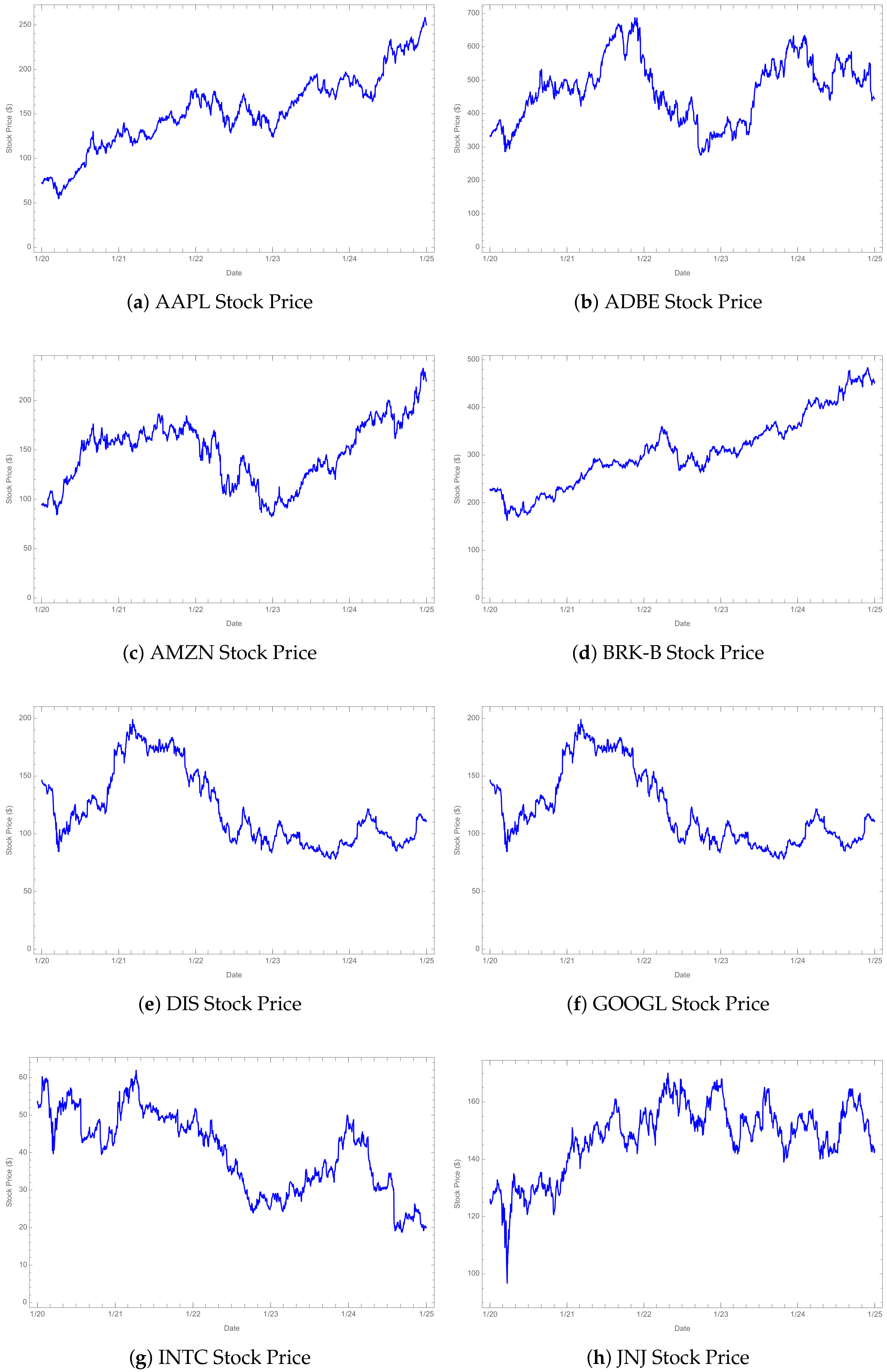
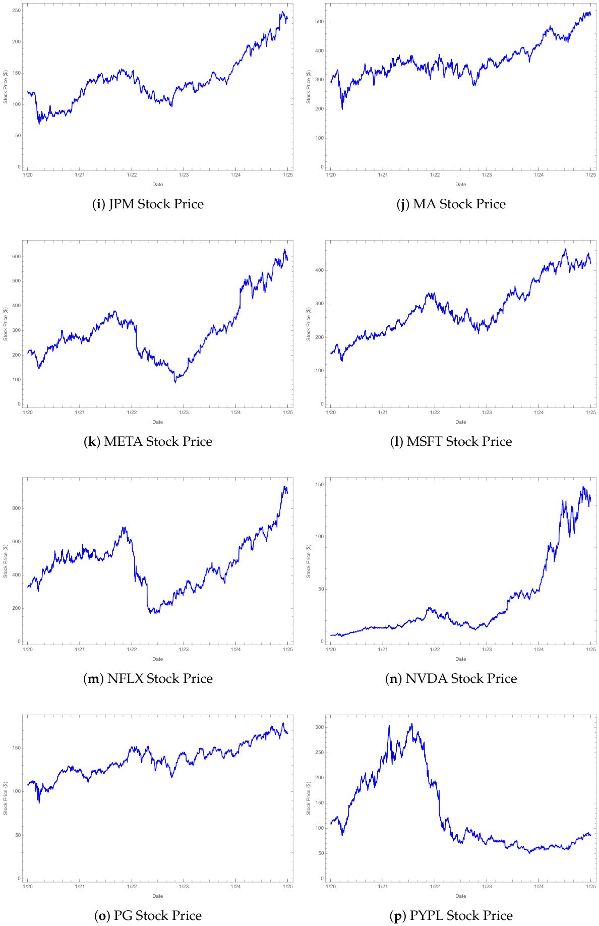
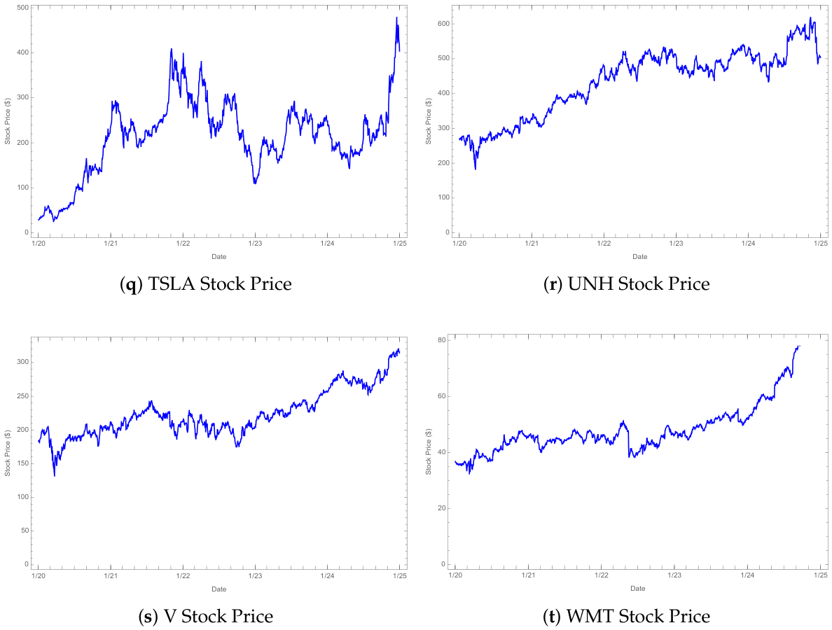
• We conduct an empirical study using daily stock price data from twenty companies in the $S\&P$ 500 index. The parameters of the MBS model are estimated using the maximum likelihood framework of Aït-Sahalia [22], and the resulting estimates are incorporated into the proposed covariance matrix to construct efficient frontiers under realistic market conditions.

The results suggest that the proposed covariance framework provides a viable alternative to purely sample-based covariance estimation and may offer a more robust basis for portfolio construction within the mean–variance optimization setting. The numerical investigations highlight the sensitivity of portfolio optimization to covariance estimation procedures, whereas the empirical study demonstrates the practical applicability of the proposed methodology using real market data. Moreover, the analytical framework developed in this paper can potentially be extended to more sophisticated asset price models, including those incorporating stochastic volatility, jump components, or alternative dependence structures.

The remainder of this paper is organized as follows. Section 2 reviews the classical Markowitz mean–variance framework, including the formulations of portfolio return, portfolio variance, and the associated portfolio optimization problems, together with conventional covariance estimation methods based on historical data. Section 3 introduces the MBS model with deterministic time-varying parameters and derives the corresponding closed-form covariance matrix, optimal portfolio allocations, and efficient frontier. Section 4 presents numerical examples and MC experiments to validate the proposed analytical framework. Section 5 demonstrates the empirical implementation of the proposed framework using data from the S&P 500 index. Section 6 discusses the limitations of the proposed methodology and outlines potential directions for future research. Finally, Section 7 concludes the paper.

2. Markowitz Model

2.1. Portfolio Wealth, Returns, and Risk Measures

Consider a financial market consisting of $n\ge 2$ risky assets observed over a fixed investment horizon $[0,T]$, where $T>0$. Let $(\mathrm{\Omega },\mathcal{F},\mathbb{P})$ be a probability space equipped with a filtration ${\left({\mathcal{F}}_t\right)}_{t\ge 0}$ satisfying the usual conditions. We denote by

$${\mathit{S}}_T=\left(S_T^{\left(1\right)},\dots ,S_T^{\left(n\right)}\right)$$

the vector of asset prices at time T, where $S_T^{\left(i\right)}$ represents the price of asset i for $i=1,\dots ,n$.

Let

$$\mathit{x}=(x_1,\dots ,x_n)\in {\left({\mathbb{R}}_0^{+}\right)}^n$$

denote a portfolio, where $x_i$ represents the number of shares held in asset i. The total wealth of an investor holding the portfolio $\mathit{x}$ at time T is given by

$$\begin{array}{c}\hfill V_T:={\mathit{S}}_T{\mathit{x}}^{\top }={\displaystyle \sum _{i=1}^n}{x}_i{S}_T^{\left(i\right)},\end{array}$$

(1)

where the initial asset price vector

$${\mathit{S}}_0=\left(S_0^{\left(1\right)},\dots ,S_0^{\left(n\right)}\right)\in {\left({\mathbb{R}}^{+}\right)}^n$$

is assumed to be known.

Suppose that the investor allocates an initial wealth $v_0>0$ at time $t=0$. Then,

$$\begin{array}{c}\hfill V_0=v_0.\end{array}$$

(2)

Define the portfolio weights by

$$\begin{array}{c}\hfill w_i:={\displaystyle \frac{x_i{S}_0^{\left(i\right)}}{v_0}},i=1,\dots ,n.\end{array}$$

(3)

The quantity $w_i$ represents the proportion of the initial wealth invested in asset i. Using (2) and (3), the wealth process in (1) can be rewritten as

$$\begin{array}{c}\hfill V_T={\displaystyle \sum _{i=1}^n}{\displaystyle \frac{v_0{w}_i}{S_0^{\left(i\right)}}}{S}_T^{\left(i\right)}.\end{array}$$

(4)

Since the entire initial wealth is invested in the portfolio, the budget constraint becomes

$$\begin{array}{c}\hfill \mathit{u}{\mathit{w}}^{\top }={\displaystyle \sum _{i=1}^n}{w}_i=1,\end{array}$$

(5)

where

$$\mathit{w}=(w_1,\dots ,w_n)$$

is the vector of portfolio weights and

$$\mathit{u}=(1,\dots ,1)\in {\mathbb{R}}^n.$$

Without loss of generality, we normalize the initial wealth by setting $v_0=1$. We further introduce the normalized asset prices

$$\begin{array}{c}\hfill {\overline{S}}_T^{\left(i\right)}:={\displaystyle \frac{S_T^{\left(i\right)}}{S_0^{\left(i\right)}}},i=1,\dots ,n,\end{array}$$

(6)

and define

$${\overline{\mathit{S}}}_T=\left({\overline{S}}_T^{\left(1\right)},\dots ,{\overline{S}}_T^{\left(n\right)}\right).$$

The quantities ${\overline{S}}_T^{\left(i\right)}$ represent the gross returns of the individual assets over the investment horizon and are introduced primarily for analytical convenience in the subsequent derivations.

Substituting (6) into (4), the total wealth process can be expressed as

$$\begin{array}{c}\hfill V_T\left(\mathit{w}\right):={\overline{\mathit{S}}}_T{\mathit{w}}^{\top }={\displaystyle \sum _{i=1}^n}{w}_i{\overline{S}}_T^{\left(i\right)}.\end{array}$$

(7)

The wealth process $V_T\left(\mathit{w}\right)$ is an ${\mathcal{F}}_T$-measurable random variable.

The gross portfolio return over the investment horizon is defined by

$$\begin{array}{c}\hfill R_T:={\displaystyle \frac{V_T-V_0}{V_0}}.\end{array}$$

(8)

Using (2) and (7), the portfolio return can be written as

$$\begin{array}{c}\hfill R_T\left(\mathit{w}\right)={\overline{\mathit{S}}}_T{\mathit{w}}^{\top }-1={\displaystyle \sum _{i=1}^n}{w}_i{\overline{S}}_T^{\left(i\right)}-1.\end{array}$$

(9)

The return $R_T\left(\mathit{w}\right)$ is also an ${\mathcal{F}}_T$-measurable random variable.

We define the expected portfolio return by

$$\begin{array}{c}\hfill {\mu }_P(T,\mathit{w},{\mathit{S}}_0):={\mathbb{E}}_0\left[R_T\left(\mathit{w}\right)\right]:={\mathbb{E}}^{\mathbb{P}}\left[R_T\left(\mathit{w}\right)\mid {\mathcal{F}}_0\right],\end{array}$$

(10)

where ${\mathbb{E}}_0[·]$ denotes conditional expectation given the information available at the initial time. The quantity ${\mu }_P(T,\mathit{w},{\mathit{S}}_0)$ represents the expected return of the portfolio over the investment horizon.

Similarly, the portfolio variance is defined as

$$\begin{array}{c}\hfill {\sigma }_P^2(T,\mathit{w},{\mathit{S}}_0):={\mathbb{VAR}}_0\left[R_T\left(\mathit{w}\right)\right]:={\mathbb{E}}_0\left[{\left(R_T\left(\mathit{w}\right)-{\mu }_P(T,\mathit{w},{\mathit{S}}_0)\right)}^2\right].\end{array}$$

(11)

Applying the linearity of expectation to (9) yields

$$\begin{array}{c}\hfill {\mu }_P(T,\mathit{w},{\mathit{S}}_0)=\overline{\mathit{M}}(T,{\mathit{S}}_0){\mathit{w}}^{\top }-1,\end{array}$$

(12)

where

$$\begin{array}{c}\hfill \overline{\mathit{M}}(T,{\mathit{S}}_0):=\left({\overline{m}}_1(T,S_0^{\left(1\right)}),\dots ,{\overline{m}}_n(T,S_0^{\left(n\right)})\right),\end{array}$$

(13)

with

$$\begin{array}{c}\hfill {\overline{m}}_i(T,S_0^{\left(i\right)}):={\mathbb{E}}_0\left[{\overline{S}}_T^{\left(i\right)}\right]={\displaystyle \frac{1}{S_0^{\left(i\right)}}}{m}_i(T,S_0^{\left(i\right)}),\end{array}$$

(14)

and

$$\begin{array}{c}\hfill m_i(T,S_0^{\left(i\right)}):={\mathbb{E}}_0\left[S_T^{\left(i\right)}\right],i=1,\dots ,n.\end{array}$$

(15)

Furthermore, using the properties of variance, we obtain

$$\begin{array}{cc}\hfill {\sigma }_P^2(T,\mathit{w},{\mathit{S}}_0)& ={\mathbb{VAR}}_0\left[{\overline{\mathit{S}}}_T{\mathit{w}}^{\top }\right]\hfill \\ \hfill & =\mathit{w}\overline{\mathit{C}}(T,{\mathit{S}}_0){\mathit{w}}^{\top },\hfill \end{array}$$

(16)

where

$$\begin{array}{c}\hfill \overline{\mathit{C}}(T,{\mathit{S}}_0):={\left[{\overline{C}}_{ij}(T,S_0^{\left(i\right)},S_0^{\left(j\right)})\right]}_{n\times n}\end{array}$$

(17)

denotes the covariance matrix of the normalized asset prices ${\overline{\mathit{S}}}_T$, with entries

$$\begin{array}{cc}\hfill {\overline{C}}_{ij}(T,S_0^{\left(i\right)},S_0^{\left(j\right)})& :={\mathbb{E}}_0\left[\left({\overline{S}}_T^{\left(i\right)}-{\overline{m}}_i(T,S_0^{\left(i\right)})\right)\left({\overline{S}}_T^{\left(j\right)}-{\overline{m}}_j(T,S_0^{\left(j\right)})\right)\right]\hfill \\ \hfill & ={\displaystyle \frac{C_{ij}(T,S_0^{\left(i\right)},S_0^{\left(j\right)})}{S_0^{\left(i\right)}{S}_0^{\left(j\right)}}},\hfill \end{array}$$

(18)

where

$$\begin{array}{c}\hfill C_{ij}(T,S_0^{\left(i\right)},S_0^{\left(j\right)}):={\mathbb{E}}_0\left[\left(S_T^{\left(i\right)}-m_i(T,S_0^{\left(i\right)})\right)\left(S_T^{\left(j\right)}-m_j(T,S_0^{\left(j\right)})\right)\right],\end{array}$$

(19)

for $i,j=1,\dots ,n$.

The covariance matrix $\overline{\mathit{C}}(T,{\mathit{S}}_0)$ plays a central role in the Markowitz framework, since it completely determines the portfolio variance through (16). In practical applications, however, the quantities appearing in (19) are generally unknown and must be estimated from historical market data. Traditional implementations of mean–variance optimization therefore rely on sample covariance estimators, which may be sensitive to finite-sample variability and estimation error. In the subsequent sections, we develop a model-driven alternative by deriving an explicit closed-form covariance matrix under an MBS model with time-varying parameters.

2.2. Minimum-Variance Portfolio Under the Budget Constraint

A fundamental problem in the Markowitz mean–variance framework is the determination of the portfolio that minimizes risk without imposing any target expected return requirement. This portfolio, commonly referred to as the global minimum-variance (GMV) portfolio, depends solely on the covariance structure of asset returns and therefore avoids the additional uncertainty associated with return forecasting.

Using the variance expression derived in (16), the minimum-variance portfolio optimization problem can be formulated as

$$\begin{array}{cc}\hfill \underset{\mathit{w}\in {\mathbb{R}}^n}{\mathrm{minimize}}& {\sigma }_P^2(T,\mathit{w},{\mathit{S}}_0)=\mathit{w}\overline{\mathit{C}}(T,{\mathit{S}}_0){\mathit{w}}^{\top }\hfill \end{array}$$

(20)

$$\begin{array}{cc}\hfill \mathrm{subject} \mathrm{to}& \mathit{u}{\mathit{w}}^{\top }=1,\hfill \end{array}$$

(21)

where

$$\mathit{u}=(1,\dots ,1)\in {\mathbb{R}}^n$$

enforces the budget constraint, ensuring that the entire initial wealth is allocated among the available assets.

We assume throughout that the covariance matrix

$$\overline{\mathit{C}}(T,{\mathit{S}}_0)$$

is positive definite. This assumption guarantees that the optimization problem admits a unique solution and that the inverse covariance matrix exists.

To solve (20) and (21), we introduce the Lagrangian function

$$\begin{array}{c}\hfill \mathcal{L}(\mathit{w},\lambda )=\mathit{w}\overline{\mathit{C}}(T,{\mathit{S}}_0){\mathit{w}}^{\top }+\lambda \left(\mathit{u}{\mathit{w}}^{\top }-1\right),\end{array}$$

(22)

where $\lambda \in \mathbb{R}$ is the Lagrange multiplier associated with the budget constraint.

Taking the gradient of (22) with respect to the portfolio weights yields the first-order condition

$$\begin{array}{c}\hfill 2\overline{\mathit{C}}(T,{\mathit{S}}_0){\mathit{w}}^{\top }+\lambda {\mathit{u}}^{\top }=\mathbf{0}.\end{array}$$

(23)

Since $\overline{\mathit{C}}(T,{\mathit{S}}_0)$ is invertible, solving (23) gives

$$\begin{array}{c}\hfill {\mathit{w}}^{\top }=-{\displaystyle \frac{\lambda }{2}}{\overline{\mathit{C}}}^{-1}(T,{\mathit{S}}_0){\mathit{u}}^{\top }.\end{array}$$

(24)

Substituting (24) into the budget constraint (21) yields

$$\begin{array}{c}\hfill -{\displaystyle \frac{\lambda }{2}}\mathit{u}{\overline{\mathit{C}}}^{-1}(T,{\mathit{S}}_0){\mathit{u}}^{\top }=1.\end{array}$$

(25)

Therefore,

$$\begin{array}{c}\hfill \lambda =-{\displaystyle \frac{2}{\mathit{u}{\overline{\mathit{C}}}^{-1}(T,{\mathit{S}}_0){\mathit{u}}^{\top }}}.\end{array}$$

(26)

Substituting (26) into (24), we obtain the optimal portfolio weights corresponding to the global minimum-variance portfolio:

$$\begin{array}{c}\hfill {\mathit{w}}^{*}={\displaystyle \frac{\mathit{u}{\overline{\mathit{C}}}^{-1}(T,{\mathit{S}}_0)}{\mathit{u}{\overline{\mathit{C}}}^{-1}(T,{\mathit{S}}_0){\mathit{u}}^{\top }}}.\end{array}$$

(27)

Since the covariance matrix is assumed to be positive definite, the objective function

$$\mathit{w}\overline{\mathit{C}}(T,{\mathit{S}}_0){\mathit{w}}^{\top }$$

is strictly convex. Consequently, the stationary point characterized by (27) is the unique global minimizer of the optimization problem (20) and (21).

The corresponding minimum portfolio variance is obtained by substituting (27) into (16), yielding

$$\begin{array}{c}\hfill {\sigma }_{\mathrm{GMV}}^2(T,{\mathit{S}}_0)={\displaystyle \frac{1}{\mathit{u}{\overline{\mathit{C}}}^{-1}(T,{\mathit{S}}_0){\mathit{u}}^{\top }}}.\end{array}$$

(28)

The global minimum-variance portfolio depends exclusively on the covariance structure of the underlying assets and is independent of their expected returns. This feature makes the GMV portfolio attractive in practice, since covariance matrices are often estimated more reliably than expected returns. Nevertheless, many investors seek portfolios that achieve a prescribed level of expected return while simultaneously minimizing risk. This consideration motivates the classical mean–variance optimization problem, which is discussed in the following subsection.

2.3. Mean–Variance Portfolio with a Target Expected Return

Although the global minimum-variance portfolio provides the lowest attainable risk among all feasible portfolios, investors often seek portfolios that satisfy a prescribed expected return requirement. This leads to the classical mean–variance optimization problem introduced by Markowitz [1,2], in which portfolio variance is minimized subject to both a budget constraint and a target expected return.

Using the expected return and variance expressions derived in (12) and (16), respectively, we consider the following optimization problem:

$$\begin{array}{cc}\hfill \underset{\mathit{w}\in {\mathbb{R}}^n}{\mathrm{minimize}}& {\sigma }_P^2(T,\mathit{w},{\mathit{S}}_0)=\mathit{w}\overline{\mathit{C}}(T,{\mathit{S}}_0){\mathit{w}}^{\top }\hfill \end{array}$$

(29)

$$\begin{array}{cc}\hfill \mathrm{subject} \mathrm{to}& \mathit{u}{\mathit{w}}^{\top }=1,\hfill \end{array}$$

(30)

$$\begin{array}{cc}\hfill & {\mu }_P(T,\mathit{w},{\mathit{S}}_0)={\mu }_0,\hfill \end{array}$$

(31)

where ${\mu }_0\in \mathbb{R}$ denotes the target expected return specified by the investor.

Using (12), the return constraint (31) can be rewritten as

$$\begin{array}{c}\hfill \overline{\mathit{M}}(T,{\mathit{S}}_0){\mathit{w}}^{\top }=1+{\mu }_0.\end{array}$$

(32)

Introducing Lagrange multipliers ${\lambda }_1,{\lambda }_2\in \mathbb{R}$ associated with constraints (30) and (32), respectively, we define the Lagrangian function

$$\begin{array}{c}\hfill \mathcal{L}(\mathit{w},{\lambda }_1,{\lambda }_2)=\mathit{w}\overline{\mathit{C}}(T,{\mathit{S}}_0){\mathit{w}}^{\top }+{\lambda }_1\left(\mathit{u}{\mathit{w}}^{\top }-1\right)+{\lambda }_2\left(\overline{\mathit{M}}(T,{\mathit{S}}_0){\mathit{w}}^{\top }-(1+{\mu }_0)\right).\end{array}$$

(33)

Taking the gradient of (33) with respect to $\mathit{w}$ and setting it equal to zero yields the first-order condition

$$\begin{array}{c}\hfill 2\overline{\mathit{C}}(T,{\mathit{S}}_0){\mathit{w}}^{\top }+{\lambda }_1{\mathit{u}}^{\top }+{\lambda }_2{\overline{\mathit{M}}}^{\top }(T,{\mathit{S}}_0)=\mathbf{0}.\end{array}$$

(34)

Since $\overline{\mathit{C}}(T,{\mathit{S}}_0)$ is invertible, solving (34) gives

$$\begin{array}{c}\hfill {\mathit{w}}^{\top }=-{\displaystyle \frac{{\lambda }_1}{2}}{\overline{\mathit{C}}}^{-1}(T,{\mathit{S}}_0){\mathit{u}}^{\top }-{\displaystyle \frac{{\lambda }_2}{2}}{\overline{\mathit{C}}}^{-1}(T,{\mathit{S}}_0){\overline{\mathit{M}}}^{\top }(T,{\mathit{S}}_0).\end{array}$$

(35)

For notational convenience, define

$$\begin{array}{c}a:=\mathit{u}{\overline{\mathit{C}}}^{-1}(T,{\mathit{S}}_0){\mathit{u}}^{\top },\hfill \end{array}$$

(36)

$$\begin{array}{c}b:=\mathit{u}{\overline{\mathit{C}}}^{-1}(T,{\mathit{S}}_0){\overline{\mathit{M}}}^{\top }(T,{\mathit{S}}_0),\hfill \end{array}$$

(37)

$$\begin{array}{c}c:=\overline{\mathit{M}}(T,{\mathit{S}}_0){\overline{\mathit{C}}}^{-1}(T,{\mathit{S}}_0){\overline{\mathit{M}}}^{\top }(T,{\mathit{S}}_0).\hfill \end{array}$$

(38)

Substituting (35) into the constraints (30) and (32) yields the linear system

$$\begin{array}{c}\hfill \left\{\begin{array}{c}-{\displaystyle \frac{{\lambda }_1}{2}}a-{\displaystyle \frac{{\lambda }_2}{2}}b=1,\hfill \\ -{\displaystyle \frac{{\lambda }_1}{2}}b-{\displaystyle \frac{{\lambda }_2}{2}}c=1+{\mu }_0.\hfill \end{array}\right.\end{array}$$

(39)

Introducing the coefficients

$$\begin{array}{c}\hfill \alpha :=-{\displaystyle \frac{{\lambda }_1}{2}},\beta :=-{\displaystyle \frac{{\lambda }_2}{2}},\end{array}$$

(40)

the system (39) can be rewritten as

$$\begin{array}{c}\hfill \left\{\begin{array}{c}a\alpha +b\beta =1,\hfill \\ b\alpha +c\beta =1+{\mu }_0.\hfill \end{array}\right.\end{array}$$

(41)

Solving (41) yields

$$\begin{array}{c}\hfill \alpha ={\displaystyle \frac{c-b(1+{\mu }_0)}{ac-b^2}},\end{array}$$

(42)

and

$$\begin{array}{c}\hfill \beta ={\displaystyle \frac{a(1+{\mu }_0)-b}{ac-b^2}}.\end{array}$$

(43)

Substituting (42) and (43) into (35), we obtain the optimal portfolio weights:

$$\begin{array}{c}\hfill {\mathit{w}}^{*}=\alpha {\overline{\mathit{C}}}^{-1}(T,{\mathit{S}}_0){\mathit{u}}^{\top }+\beta {\overline{\mathit{C}}}^{-1}(T,{\mathit{S}}_0){\overline{\mathit{M}}}^{\top }(T,{\mathit{S}}_0).\end{array}$$

(44)

Since the covariance matrix $\overline{\mathit{C}}(T,{\mathit{S}}_0)$ is assumed to be positive definite, the objective function in (29) is strictly convex. Consequently, the portfolio weights given by (44) constitute the unique global minimizer of the optimization problem (29)–(31).

The solution (44) characterizes the mean–variance efficient portfolio corresponding to the prescribed target return ${\mu }_0$. As the target return varies over the set of attainable values, the associated minimum-variance portfolios trace out the efficient frontier, representing the set of portfolios that achieve the lowest possible risk for each level of expected return.

The explicit characterization of the efficient frontier plays a fundamental role in portfolio selection, as it enables investors to identify portfolios that best align with their individual risk preferences. The construction and properties of the efficient frontier are discussed in the next subsection.

2.4. Efficient Frontier

The concept of the efficient frontier is fundamental to the Markowitz mean–variance framework, as it characterizes the optimal trade-off between expected return and risk. Building on the portfolio return and variance measures introduced in Section 2.1, each admissible portfolio weight vector

$$\mathit{w}=(w_1,\dots ,w_n)$$

determines a pair

$$\left({\sigma }_P(T,\mathit{w},{\mathit{S}}_0),{\mu }_P(T,\mathit{w},{\mathit{S}}_0)\right),$$

where

$${\mu }_P(T,\mathit{w},{\mathit{S}}_0)$$

denotes the expected portfolio return defined in (10), and

$${\sigma }_P(T,\mathit{w},{\mathit{S}}_0)=\sqrt{{\sigma }_P^2(T,\mathit{w},{\mathit{S}}_0)}$$

represents the corresponding portfolio risk measured by the standard deviation of returns.

As the portfolio weights vary over the set

$$\mathcal{W}=\left\{\mathit{w}\in {\mathbb{R}}^n:\mathit{u}{\mathit{w}}^{\top }=1\right\},$$

the resulting collection of risk–return pairs forms a region in the $({\sigma }_P,{\mu }_P)$-plane, commonly referred to as the feasible set. This set contains all portfolios that satisfy the budget constraint and therefore represents all attainable combinations of expected return and risk available to investors.

Among the portfolios contained in the feasible set, particular attention is devoted to those that achieve the lowest possible level of risk for a given expected return. These portfolios constitute the efficient frontier.

Definition 1.

The efficient frontier is defined as the set of portfolios that solve the optimization problem

$$\begin{array}{cc}\hfill \underset{\mathit{w}\in {\mathbb{R}}^n}{\mathrm{minimize}}& {\sigma }_P^2(T,\mathit{w},{\mathit{S}}_0)\hfill \\ \hfill subject to& {\mu }_P(T,\mathit{w},{\mathit{S}}_0)={\mu }_0,\hfill \\ \hfill & \mathit{u}{\mathit{w}}^{\top }=1,\hfill \end{array}$$

(45)

for all feasible values of the target expected return ${\mu }_0$.

Equivalently, the efficient frontier may be viewed as the upper boundary of the feasible set in the mean–variance plane. Portfolios located below this boundary are considered inefficient because there exist alternative portfolios that achieve a higher expected return for the same level of risk, or equivalently, a lower level of risk for the same expected return.

A special point on the efficient frontier is the global minimum-variance portfolio derived in Section 2.2. This portfolio attains the smallest achievable variance among all feasible portfolios and therefore represents the leftmost point on the efficient frontier. Its portfolio weights are given by

$$\begin{array}{c}\hfill {\mathit{w}}_{\mathrm{GMV}}={\displaystyle \frac{\mathit{u}{\overline{\mathit{C}}}^{-1}(T,{\mathit{S}}_0)}{\mathit{u}{\overline{\mathit{C}}}^{-1}(T,{\mathit{S}}_0){\mathit{u}}^{\top }}},\end{array}$$

(46)

with corresponding variance

$$\begin{array}{c}\hfill {\sigma }_{\mathrm{GMV}}^2(T,{\mathit{S}}_0)={\displaystyle \frac{1}{\mathit{u}{\overline{\mathit{C}}}^{-1}(T,{\mathit{S}}_0){\mathit{u}}^{\top }}}.\end{array}$$

(47)

Although the global minimum-variance portfolio is optimal from the perspective of risk minimization, it does not necessarily provide the highest attainable expected return. Investors with different attitudes toward risk may therefore select alternative portfolios located along the efficient frontier.

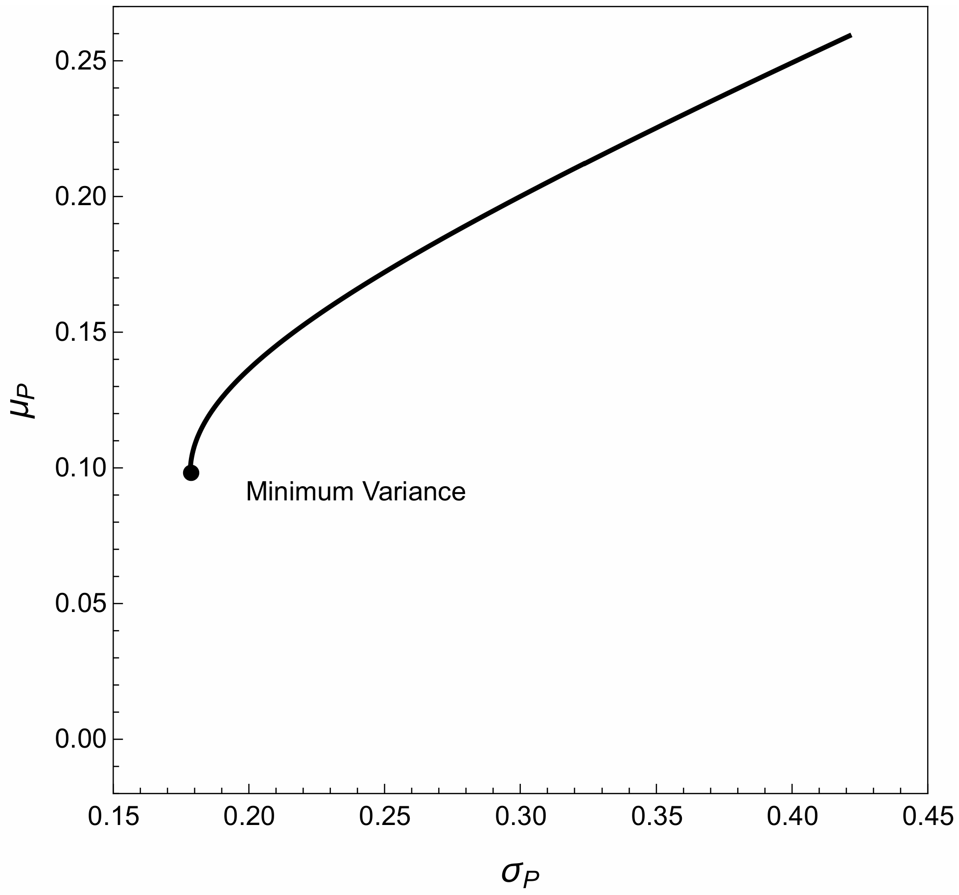
Under the standard assumptions of the Markowitz framework, including the positive definiteness of the covariance matrix, the efficient frontier exhibits a parabolic shape in the $({\sigma }_P,{\mu }_P)$-plane. The lower branch of this parabola corresponds to inefficient portfolios, whereas the upper branch consists of portfolios that satisfy the mean–variance efficiency criterion. Figure 1 provides a graphical illustration of the feasible set and the efficient frontier.

The efficient frontier provides a convenient framework for portfolio selection. More risk-averse investors tend to choose portfolios located near the global minimum-variance portfolio, whereas investors with a greater tolerance for risk may prefer portfolios associated with higher expected returns. Consequently, the efficient frontier serves as a fundamental tool for understanding the relationship between risk and return in portfolio optimization.

The theoretical developments presented thus far assume that the expected returns and covariance matrix are known quantities. In practice, however, these parameters are not directly observable and must be estimated using historical market data. The next subsection therefore reviews the conventional estimation procedures commonly employed in empirical implementations of the Markowitz framework.

2.5. Expected Return and Covariance Estimation

The theoretical development presented in the preceding subsections assumes that the expected return vector and covariance matrix are known. In practical applications, however, these quantities are unobservable and must be estimated from historical market data. The resulting estimates serve as the principal inputs for empirical implementations of the Markowitz mean–variance framework.

Let

$${\left\{S_t^{\left(i\right)}\right\}}_{t=-N}^0,i=1,\dots ,n,$$

denote the observed historical prices of asset i, where $t=0$ represents the present time and N denotes the number of past observations available for estimation.

To maintain consistency with the normalized asset prices introduced in Section 2.1, we first consider the corresponding gross returns. The gross return of asset i over the interval $(t-1,t]$ is defined as

$$\begin{array}{c}\hfill G_t^{\left(i\right)}={\displaystyle \frac{S_t^{\left(i\right)}}{S_{t-1}^{\left(i\right)}}},t=-N+1,\dots ,0.\end{array}$$

(48)

Let

$${\mathit{G}}_t=\left(G_t^{\left(1\right)},\dots ,G_t^{\left(n\right)}\right)$$

denote the vector of gross returns at time t. The corresponding sample mean gross return vector is given by

$$\begin{array}{c}\hfill \overline{\mathit{G}}={\displaystyle \frac{1}{N}}{\displaystyle \sum _{t=-N+1}^0}{\mathit{G}}_t.\end{array}$$

(49)

Since

$${\displaystyle \frac{S_1^{\left(i\right)}}{S_0^{\left(i\right)}}}$$

represents the one-period gross return over the investment horizon considered in the theoretical model, a natural estimator for the vector

$$\overline{\mathit{M}}(T,{\mathit{S}}_0)$$

defined in (13) is

$$\begin{array}{c}\hfill \widehat{\overline{\mathit{M}}}(T,{\mathit{S}}_0)=\overline{\mathit{G}}.\end{array}$$

(50)

Substituting (50) into (12), the estimator of the expected portfolio return becomes

$$\begin{array}{c}\hfill {\widehat{\mu }}_P(T,\mathit{w},{\mathit{S}}_0)=\overline{\mathit{G}}{\mathit{w}}^{\top }-1.\end{array}$$

(51)

For empirical applications, it is often more convenient to work with simple returns. Accordingly, we define the simple return of asset i at time t by

$$\begin{array}{c}\hfill R_t^{\left(i\right)}=G_t^{\left(i\right)}-1,t=-N+1,\dots ,0.\end{array}$$

(52)

Let

$${\mathit{R}}_t=\left(R_t^{\left(1\right)},\dots ,R_t^{\left(n\right)}\right)$$

denote the vector of simple returns. The sample mean simple return vector is then given by

$$\begin{array}{c}\hfill \overline{\mathit{R}}={\displaystyle \frac{1}{N}}{\displaystyle \sum _{t=-N+1}^0}{\mathit{R}}_t=\overline{\mathit{G}}-\mathit{u},\end{array}$$

(53)

where

$$\mathit{u}=(1,\dots ,1)\in {\mathbb{R}}^n.$$

Combining (51) and (53), the estimated portfolio expected return can equivalently be expressed as

$$\begin{array}{c}\hfill {\widehat{\mu }}_P(T,\mathit{w},{\mathit{S}}_0)=\overline{\mathit{R}}{\mathit{w}}^{\top }.\end{array}$$

(54)

The covariance matrix of asset returns is commonly estimated using the sample covariance matrix constructed from historical simple returns. Specifically, the sample covariance matrix is defined by

$$\begin{array}{c}\hfill \widehat{\mathit{C}}={\displaystyle \frac{1}{N-1}}{\displaystyle \sum _{t=-N+1}^0}{\left({\mathit{R}}_t-\overline{\mathit{R}}\right)}^{\top }\left({\mathit{R}}_t-\overline{\mathit{R}}\right).\end{array}$$

(55)

The estimator (55) provides an unbiased estimate of the covariance matrix under the assumption that the observed return vectors are independently and identically distributed with finite second moments. Using (55), the estimated portfolio variance is given by

$$\begin{array}{c}\hfill {\widehat{\sigma }}_P^2(T,\mathit{w},{\mathit{S}}_0)=\mathit{w}\widehat{\mathit{C}}{\mathit{w}}^{\top }.\end{array}$$

(56)

The estimators (54) and (56) constitute the standard empirical inputs used in practical implementations of the Markowitz framework. Nevertheless, several limitations of these estimators have been documented in the literature. In particular, the sample covariance matrix may exhibit substantial estimation variability when the number of observations is limited relative to the number of assets. Furthermore, since mean–variance optimization depends explicitly on the inverse covariance matrix, even relatively small perturbations in covariance estimates can be amplified through the optimization procedure, resulting in unstable portfolio allocations and poor out-of-sample performance [3,8,9,23].

These limitations have motivated the development of alternative covariance estimation procedures, including shrinkage estimators, factor models, Bayesian approaches, and robust optimization techniques. In this paper, we pursue a different direction by deriving a model-driven covariance matrix directly from an underlying multidimensional stochastic asset pricing model. The resulting covariance structure provides an analytical alternative to traditional sample covariance estimation and forms the foundation of the portfolio optimization framework developed in the subsequent sections.

In the next section, we introduce an MBS model with time-varying parameters and derive an explicit closed-form expression for the corresponding covariance matrix. This model-implied covariance structure will subsequently be incorporated into the Markowitz framework to obtain analytical expressions for optimal portfolio weights and the efficient frontier.

3. Markowitz Portfolio Optimization Under a Multidimensional Black–Scholes Model with Time-Varying Parameters

Section 2 reviewed the classical Markowitz mean–variance framework and the conventional procedures used to estimate expected returns and covariance matrices from historical market data. As discussed therein, empirical implementations of portfolio optimization are often sensitive to the choice of covariance estimator, particularly when the available sample size is limited or market conditions evolve over time.

To address these challenges, we adopt a model-driven approach in which the dynamics of asset prices are specified explicitly through an MBS model with time-varying parameters. Within this framework, we derive a closed-form expression for the covariance matrix of normalized asset prices introduced in Section 2. The resulting covariance structure can then be incorporated directly into the Markowitz optimization framework to obtain analytical representations of optimal portfolio allocations and the associated efficient frontier.

The remainder of this section is organized as follows. Section 3.1 introduces the MBS model with time-varying parameters. Section 3.2 derives the closed-form covariance matrix under the proposed model. Section 3.3 incorporates the resulting covariance structure into the Markowitz framework to characterize the corresponding optimal portfolio allocations. Finally, Section 3.4 presents the efficient frontier implied by the proposed model.

3.1. Multidimensional Black–Scholes Model with Time-Varying Parameters

In this subsection, we introduce the MBS model with time-varying parameters that forms the basis of the model-driven covariance structure developed in the subsequent subsection.

Let

$$(\mathrm{\Omega },\mathcal{F},\mathbb{P})$$

be a probability space equipped with a filtration

$${\left({\mathcal{F}}_t\right)}_{t\ge 0}$$

satisfying the usual conditions. Consider a financial market consisting of d risky assets, whose price processes are denoted by

$$S_t^{\left(i\right)},i=1,\dots ,d.$$

We assume that the asset price dynamics evolve according to the MBS model with time-varying coefficients:

$$\begin{array}{c}\hfill d{S}_t^{\left(i\right)}=S_t^{\left(i\right)}\left({\mu }_i\left(t\right)dt+{\sigma }_i\left(t\right)d{W}_t^{\left(i\right)}\right),S_0^{\left(i\right)}>0,\end{array}$$

(57)

for $i=1,\dots ,d$, where

• ${\mu }_i:[0,T]\to \mathbb{R}$ is a deterministic continuous drift function of asset i;
• ${\sigma }_i:[0,T]\to (0,\infty )$ is a deterministic continuous volatility function of asset i;
• $W_t^{\left(i\right)}$, $i=1,\dots ,d$, are one-dimensional Brownian motions defined on $(\mathrm{\Omega },\mathcal{F},\mathbb{P})$.

The dependence structure among the assets is characterized through the instantaneous correlations of the Brownian motions. Specifically, we assume that

$$\begin{array}{c}\hfill d{W}_t^{\left(i\right)}d{W}_t^{\left(j\right)}={\rho }_{ij}\left(t\right)dt,i,j=1,\dots ,d,\end{array}$$

(58)

where

$${\rho }_{ij}:[0,T]\to [-1,1]$$

is a deterministic continuous instantaneous correlation function between assets i and j. Moreover,

$${\rho }_{ii}\left(t\right)=1,i=1,\dots ,d,$$

and the matrix

$$\mathit{\rho }\left(t\right)={\left({\rho }_{ij}\left(t\right)\right)}_{d\times d}$$

is assumed to be symmetric and positive semidefinite for every $t\in [0,T]$.

The MBS model (57) generalizes the classical geometric Brownian motion framework by allowing both the drift and volatility coefficients to vary over time. This additional flexibility enables the model to capture certain forms of nonstationarity frequently observed in financial markets while preserving analytical tractability.

Applying Itô’s formula to the logarithm of the asset price process yields

$$\begin{array}{c}\hfill d\ln S_t^{\left(i\right)}=\left({\mu }_i\left(t\right)-{\displaystyle \frac{1}{2}}{\sigma }_i^2\left(t\right)\right)dt+{\sigma }_i\left(t\right)d{W}_t^{\left(i\right)},i=1,\dots ,d.\end{array}$$

(59)

Integrating (59) over the interval $[0,T]$, we obtain

$$\begin{array}{c}\hfill \ln \left({\displaystyle \frac{S_T^{\left(i\right)}}{S_0^{\left(i\right)}}}\right)={\int }_0^T\left({\mu }_i\left(s\right)-{\displaystyle \frac{1}{2}}{\sigma }_i^2\left(s\right)\right)ds+{\int }_0^T{\sigma }_i\left(s\right)d{W}_s^{\left(i\right)}.\end{array}$$

(60)

Exponentiating both sides of (60) gives the explicit representation

$$\begin{array}{c}\hfill S_T^{\left(i\right)}=S_0^{\left(i\right)}\exp \left({\int }_0^T\left({\mu }_i\left(s\right)-{\displaystyle \frac{1}{2}}{\sigma }_i^2\left(s\right)\right)ds+{\int }_0^T{\sigma }_i\left(s\right)d{W}_s^{\left(i\right)}\right),\end{array}$$

(61)

for $i=1,\dots ,d$.

The representation (61) forms the foundation for deriving the first and second moments of asset prices under the proposed model. In particular, it enables an explicit characterization of the covariance quantities introduced in Section 2, thereby providing a model-driven alternative to the conventional sample covariance estimators commonly employed in empirical portfolio optimization.

In the next subsection, we derive a closed-form expression for the covariance matrix of normalized asset prices under the multidimensional Black–Scholes model with time-varying parameters.

3.2. Closed-Form Covariance Matrix Under the Multidimensional Black–Scholes Model

The covariance matrix introduced in Section 2 constitutes the principal input in the Markowitz mean–variance framework. Under the MBS model introduced in Section 3.1, the covariance quantities can be derived analytically from the underlying asset price dynamics.

Theorem 1.

Let $S_0^{\left(i\right)},S_0^{\left(j\right)}>0$, for $i,j=1,\dots ,d$ and suppose that the asset price dynamics satisfy the MBS model (57). Then the covariance quantity defined in (19) admits the representation

$$\begin{array}{cc}\hfill C_{ij}\left(T,S_0^{\left(i\right)},S_0^{\left(j\right)}\right)& =S_0^{\left(i\right)}{S}_0^{\left(j\right)}\left(\exp \left(A_{ij}^{(1,1)}\left(T\right)\right)-\exp \left(B_i\left(T\right)\right)\exp \left(B_j\left(T\right)\right)\right),\hfill \end{array}$$

(62)

where

$$\begin{array}{cc}\hfill B_i\left(T\right)& ={\int }_0^T{\mu }_i\left(s\right)ds,\hfill \end{array}$$

(63)

and

$$\begin{array}{cc}\hfill A_{ij}^{(1,1)}\left(T\right)& ={\int }_0^T\left({\mu }_i\left(s\right)+{\mu }_j\left(s\right)+{\rho }_{ij}\left(s\right){\sigma }_i\left(s\right){\sigma }_j\left(s\right)\right)ds.\hfill \end{array}$$

(64)

Consequently, the covariance matrix of normalized asset prices introduced in (17) satisfies

$$\begin{array}{cc}\hfill {\overline{C}}_{ij}\left(T,S_0^{\left(i\right)},S_0^{\left(j\right)}\right)& =\exp \left(A_{ij}^{(1,1)}\left(T\right)\right)-\exp \left(B_i\left(T\right)\right)\exp \left(B_j\left(T\right)\right).\hfill \end{array}$$

(65)

Proof. 

The proof is provided in Appendix B.1. □

While the underlying moment calculations follow standard properties of diffusion processes, Theorem 1 expresses the covariance matrix in a form that can be directly incorporated into the Markowitz optimization framework. Consequently, the proposed approach provides a practical model-based alternative to conventional sample covariance estimation once the model parameters have been specified or estimated.

For empirical implementation, we consider the case in which the drift and volatility functions vary linearly over time and the correlation coefficients are constant.

Corollary 1.

Let $S_0^{\left(i\right)},S_0^{\left(j\right)}>0$, for $i,j=1,\dots ,d$, and suppose that

$$\begin{array}{c}\hfill {\mu }_i\left(t\right)={\mu }_{i0}+{\mu }_{i1}t,{\sigma }_i\left(t\right)={\sigma }_{i0}+{\sigma }_{i1}t,\end{array}$$

(66)

for $t\in [0,T]$ and that ${\rho }_{ij}\left(t\right)\equiv {\rho }_{ij}$. Then

$$\begin{array}{cc}\hfill C_{ij}\left(T,S_0^{\left(i\right)},S_0^{\left(j\right)}\right)& =S_0^{\left(i\right)}{S}_0^{\left(j\right)}\left(\exp \left(A_{ij}^{(1,1)}\left(T\right)\right)-\exp \left(B_i\left(T\right)\right)\exp \left(B_j\left(T\right)\right)\right),\hfill \end{array}$$

(67)

where

$$\begin{array}{cc}\hfill B_i\left(T\right)& ={\mu }_{i0}T+{\displaystyle \frac{1}{2}}{\mu }_{i1}{T}^2,\hfill \end{array}$$

(68)

and

$$\begin{array}{cc}\hfill A_{ij}^{(1,1)}\left(T\right)& =\left({\mu }_{i0}+{\mu }_{j0}+{\rho }_{ij}{\sigma }_{i0}{\sigma }_{j0}\right)T\hfill \\ \hfill & +{\displaystyle \frac{1}{2}}\left({\mu }_{i1}+{\mu }_{j1}+{\rho }_{ij}\left({\sigma }_{i0}{\sigma }_{j1}+{\sigma }_{i1}{\sigma }_{j0}\right)\right)T^2\hfill \\ \hfill & +{\displaystyle \frac{1}{3}}{\rho }_{ij}{\sigma }_{i1}{\sigma }_{j1}{T}^3.\hfill \end{array}$$

(69)

Consequently,

$$\begin{array}{cc}\hfill {\overline{C}}_{ij}\left(T,S_0^{\left(i\right)},S_0^{\left(j\right)}\right)& =\exp \left(A_{ij}^{(1,1)}\left(T\right)\right)-\exp \left(B_i\left(T\right)\right)\exp \left(B_j\left(T\right)\right).\hfill \end{array}$$

(70)

Proof. 

The proof is provided in Appendix B.2. □

The closed-form representations derived above enable the covariance matrix

$$\overline{\mathit{C}}(T,{\mathit{S}}_0)={\left[{\overline{C}}_{ij}\left(T,S_0^{\left(i\right)},S_0^{\left(j\right)}\right)\right]}_{d\times d}$$

to be constructed analytically once the model parameters have been specified or estimated. Since $\overline{\mathit{C}}(T,{\mathit{S}}_0)$ is a covariance matrix, it is positive semidefinite by construction. To ensure the existence of the inverse covariance matrix required in the subsequent portfolio optimization results, we assume throughout that $\overline{\mathit{C}}(T,{\mathit{S}}_0)$ is positive definite.

The analytical covariance structure derived in this subsection provides the key link between the MBS model and the Markowitz framework introduced in Section 2. In the next subsection, we incorporate this covariance matrix into the classical portfolio optimization problems.

3.3. Portfolio Optimization Under the Multidimensional Black-Scholes Model

The closed-form covariance matrix derived in Section 3.2 can now be incorporated directly into the Markowitz optimization framework developed in Section 2. Since the covariance quantities are available analytically, the resulting portfolio weights can be expressed explicitly in terms of the model parameters.

We first consider the global minimum-variance portfolio.

Corollary 2.

Suppose that the assumptions of Theorem 1 hold and that the covariance matrix

$$\overline{\mathit{C}}(T,{\mathit{S}}_0)$$

is positive definite. Then the global minimum-variance portfolio weights are given by

$$\begin{array}{c}\hfill {\mathit{w}}_{\mathrm{GMV}}={\displaystyle \frac{\mathit{u}{\overline{\mathit{C}}}^{-1}(T,{\mathit{S}}_0)}{\mathit{u}{\overline{\mathit{C}}}^{-1}(T,{\mathit{S}}_0){\mathit{u}}^{\top }}},\end{array}$$

(71)

where

$$\mathit{u}=(1,\dots ,1)\in {\mathbb{R}}^d.$$

Moreover, the corresponding minimum portfolio variance is

$$\begin{array}{c}\hfill {\sigma }_{\mathrm{GMV}}^2(T,{\mathit{S}}_0)={\displaystyle \frac{1}{\mathit{u}{\overline{\mathit{C}}}^{-1}(T,{\mathit{S}}_0){\mathit{u}}^{\top }}}.\end{array}$$

(72)

Proof. 

The result follows immediately from (27) and (28) by substituting the covariance matrix obtained in Theorem 1. □

The global minimum-variance portfolio depends exclusively on the covariance structure of normalized asset prices and is therefore unaffected by errors arising from the estimation of expected returns. Nevertheless, many investors seek portfolios that achieve a prescribed expected return while simultaneously minimizing risk. This leads to the classical mean–variance optimization problem.

Corollary 3.

Suppose that the assumptions of Theorem 1 hold and that

$$\overline{\mathit{C}}(T,{\mathit{S}}_0)$$

is positive definite. Let

$${\mu }_0$$

be a prescribed target expected return. Then the portfolio weights that solve

$$\begin{array}{cc}\hfill \underset{\mathit{w}\in {\mathbb{R}}^d}{\mathrm{minimize}}& \mathit{w}\overline{\mathit{C}}(T,{\mathit{S}}_0){\mathit{w}}^{\top }\hfill \\ \hfill subject to& \mathit{u}{\mathit{w}}^{\top }=1,\hfill \\ \hfill & {\mu }_P(T,\mathit{w},{\mathit{S}}_0)={\mu }_0,\hfill \end{array}$$

(73)

are given by

$$\begin{array}{c}\hfill {\mathit{w}}^{*}=\alpha {\overline{\mathit{C}}}^{-1}(T,{\mathit{S}}_0){\mathit{u}}^{\top }+\beta {\overline{\mathit{C}}}^{-1}(T,{\mathit{S}}_0){\overline{\mathit{M}}}^{\top }(T,{\mathit{S}}_0),\end{array}$$

(74)

where

$$\begin{array}{c}a=\mathit{u}{\overline{\mathit{C}}}^{-1}(T,{\mathit{S}}_0){\mathit{u}}^{\top },\hfill \end{array}$$

(75)

$$\begin{array}{c}b=\mathit{u}{\overline{\mathit{C}}}^{-1}(T,{\mathit{S}}_0){\overline{\mathit{M}}}^{\top }(T,{\mathit{S}}_0),\hfill \end{array}$$

(76)

$$\begin{array}{c}c=\overline{\mathit{M}}(T,{\mathit{S}}_0){\overline{\mathit{C}}}^{-1}(T,{\mathit{S}}_0){\overline{\mathit{M}}}^{\top }(T,{\mathit{S}}_0),\hfill \end{array}$$

(77)

and

$$\begin{array}{c}\hfill \alpha ={\displaystyle \frac{c-b(1+{\mu }_0)}{ac-b^2}},\end{array}$$

(78)

while

$$\begin{array}{c}\hfill \beta ={\displaystyle \frac{a(1+{\mu }_0)-b}{ac-b^2}}.\end{array}$$

(79)

Proof. 

The result follows directly from (44) after replacing the covariance matrix by its analytical representation derived in Section 3.2. □

Corollaries 2 and 3 demonstrate that the model-driven covariance matrix developed in Section 3.2 can be incorporated seamlessly into the classical Markowitz framework. Consequently, the optimal portfolio weights admit explicit analytical representations once the underlying model parameters have been specified or estimated.

The explicit characterization of the optimal portfolios naturally leads to the corresponding risk–return relationship implied by the proposed model. In the next subsection, we derive the efficient frontier associated with the MBS framework.

3.4. Efficient Frontier Under the Multidimensional Black–Scholes Model

The explicit characterization of the optimal portfolio weights obtained in Section 3.3 naturally leads to the description of the corresponding risk–return trade-off implied by the MBS model with time-varying parameters.

Recall the quantities

$$\begin{array}{c}a=\mathit{u}{\overline{\mathit{C}}}^{-1}(T,{\mathit{S}}_0){\mathit{u}}^{\top },\hfill \end{array}$$

(80)

$$\begin{array}{c}b=\mathit{u}{\overline{\mathit{C}}}^{-1}(T,{\mathit{S}}_0){\overline{\mathit{M}}}^{\top }(T,{\mathit{S}}_0),\hfill \end{array}$$

(81)

$$\begin{array}{c}c=\overline{\mathit{M}}(T,{\mathit{S}}_0){\overline{\mathit{C}}}^{-1}(T,{\mathit{S}}_0){\overline{\mathit{M}}}^{\top }(T,{\mathit{S}}_0),\hfill \end{array}$$

(82)

where

$$\overline{\mathit{C}}(T,{\mathit{S}}_0)$$

denotes the covariance matrix of normalized asset prices derived in Section 3.2, and

$$\overline{\mathit{M}}(T,{\mathit{S}}_0)$$

is the corresponding expected gross return vector introduced in Section 2.1.

The following proposition provides an explicit representation of the efficient frontier under the proposed framework.

Proposition 1.

Suppose that the assumptions of Theorem 1 hold and that the covariance matrix

$$\overline{\mathit{C}}(T,{\mathit{S}}_0)$$

is positive definite. Then, the efficient frontier associated with the multidimensional Black–Scholes model is characterized by

$$\begin{array}{c}\hfill {\sigma }_P^2={\displaystyle \frac{a{(1+{\mu }_P)}^2-2b(1+{\mu }_P)+c}{ac-b^2}},\end{array}$$

(83)

where

$${\mu }_P={\mu }_P(T,\mathit{w},{\mathit{S}}_0)$$

denotes the expected portfolio return.

Equivalently, since

$$1+{\mu }_P=\overline{\mathit{M}}(T,{\mathit{S}}_0){\mathit{w}}^{\top },$$

the efficient frontier may be expressed directly in terms of the gross portfolio return

$${\overline{\mu }}_P=1+{\mu }_P$$

as

$$\begin{array}{c}\hfill {\sigma }_P^2={\displaystyle \frac{a{\overline{\mu }}_P^2-2b{\overline{\mu }}_P+c}{ac-b^2}}.\end{array}$$

(84)

Proof. 

Substituting the optimal portfolio weights (74) into the portfolio variance expression

$${\sigma }_P^2(T,\mathit{w},{\mathit{S}}_0)=\mathit{w}\overline{\mathit{C}}(T,{\mathit{S}}_0){\mathit{w}}^{\top },$$

and simplifying the resulting expression yields

$$\begin{array}{c}\hfill {\sigma }_P^2={\displaystyle \frac{a{(1+{\mu }_P)}^2-2b(1+{\mu }_P)+c}{ac-b^2}}.\end{array}$$

The alternative representation (84) follows immediately from the relation

$${\overline{\mu }}_P=1+{\mu }_P.$$

This completes the proof. □

Proposition 1 establishes that the efficient frontier under the proposed model retains the familiar hyperbolic structure of the classical Markowitz framework. However, unlike the traditional setting in which the covariance matrix is estimated directly from historical returns, the coefficients appearing in (83) are determined through the analytical covariance matrix derived in Section 3.2.

Consequently, once the parameters of the MBS model have been specified or estimated, the entire efficient frontier can be constructed explicitly without repeated numerical optimization procedures. This feature facilitates sensitivity analysis, comparison with empirically estimated frontiers, and practical portfolio construction under time-varying market conditions.

4. Numerical Results and Discussions

In this section, we present a numerical investigation of the GMV portfolio under the MBS framework. In particular, we examine the impact of replacing the closed-form covariance matrix derived in Section 3.2 with a sample covariance matrix estimated from MC simulated asset price trajectories.

The analysis is divided into two main parts. First, we compare the optimal portfolio weights obtained from the analytical covariance matrix with those computed using sample covariance matrices. Second, we investigate the finite-sample behavior of the resulting portfolio allocations as the number of MC simulation paths increases.

The sample covariance matrix is a consistent estimator of the true covariance structure under the MBS model. Therefore, provided that the limiting covariance matrix is positive definite, the GMV portfolio weights constructed from the sample covariance matrix converge to those obtained from the closed-form covariance matrix as the sample size tends to infinity. Nevertheless, for finite samples, the convergence of portfolio weights may be slow because the GMV allocation depends nonlinearly on the inverse covariance matrix. Consequently, small perturbations in the covariance matrix can be amplified through the optimization procedure. The purpose of this numerical study is therefore to quantify the finite-sample sensitivity of the GMV portfolio weights under different correlation structures and portfolio dimensions.

All numerical experiments were conducted using Mathematica 13.0 on a system equipped with an Apple 2.3 GHz Dual-Core Intel Core i5 processor (8 GB RAM) running macOS Ventura 13.4.1.

4.1. Finite-Sample Variability of GMV Portfolio Weights

Example 1.

We consider a three-asset portfolio to investigate the finite-sample sensitivity of the GMV portfolio weights to covariance estimation error. The GMV portfolio weights are first computed using the closed-form covariance matrix derived under the MBS model, as described in Corollary 2. These weights serve as a benchmark for comparison.

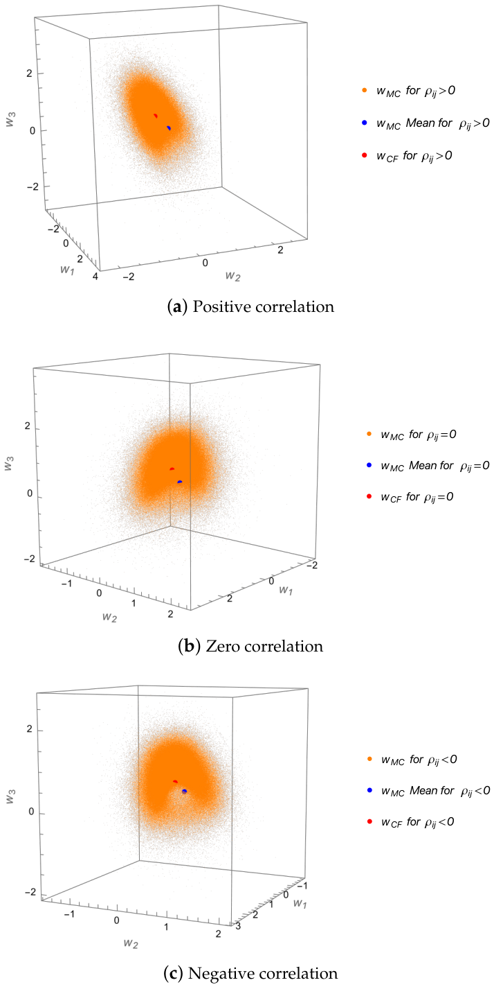
To assess the impact of covariance estimation error, we compare the benchmark weights with those obtained from sample covariance matrices estimated using MC-simulated asset price trajectories. Let

$$\overline{\mathit{C}}$$

denote the analytical covariance matrix derived in Section 3.2 and let

$${\widehat{\mathit{C}}}_N^{\left(k\right)}$$

denote the sample covariance matrix obtained from the k-th MC replication using N simulated trajectories. For each replication, the corresponding GMV portfolio weights are computed according to

$$\begin{array}{c}\hfill {\mathit{w}}_{\mathrm{MC}}^{\left(k\right)}={\displaystyle \frac{{\left({\widehat{\mathit{C}}}_N^{\left(k\right)}\right)}^{-1}\mathit{u}}{{\mathit{u}}^{\top }{\left({\widehat{\mathit{C}}}_N^{\left(k\right)}\right)}^{-1}\mathit{u}}},\end{array}$$

(85)

where

$$\mathit{u}=(1,1,1).$$

Similarly, the benchmark portfolio weights obtained from the closed-form covariance matrix are given by

$$\begin{array}{c}\hfill {\mathit{w}}_{\mathrm{CF}}={\displaystyle \frac{{\overline{\mathit{C}}}^{-1}\mathit{u}}{{\mathit{u}}^{\top }{\overline{\mathit{C}}}^{-1}\mathit{u}}}.\end{array}$$

(86)

To quantify the discrepancy between the two sets of portfolio weights, we consider the Euclidean distance

$$\begin{array}{c}\hfill d_N^{\left(k\right)}={∥{\mathit{w}}_{\mathrm{CF}}-{\mathit{w}}_{\mathrm{MC}}^{\left(k\right)}∥}_2,\end{array}$$

(87)

where

$${\parallel ·\parallel }_2$$

denotes the standard Euclidean norm.

The model parameters are chosen for illustrative purposes and are intended to reflect typical ranges of drift and volatility encountered in financial markets. Specifically, we consider

$${\mu }_{10}=0.5633,{\mu }_{11}=-0.1834,{\sigma }_{10}=0.2078,{\sigma }_{11}=0.0049,$$

$${\mu }_{20}=0.7290,{\mu }_{21}=-0.2074,{\sigma }_{20}=0.3423,{\sigma }_{21}=0.0123,$$

and

$${\mu }_{30}=-0.0061,{\mu }_{31}=0.1633,{\sigma }_{30}=0.2076,{\sigma }_{31}=-0.0147.$$

The initial asset prices are specified as

$$S_1\left(0\right)=10,S_2\left(0\right)=5,S_3\left(0\right)=7.$$

The investment horizon is taken to be

$$T=1,$$

and the asset price dynamics are simulated using 252 time steps with $N={10}^6$ MC trajectories.

To examine the influence of the dependence structure, we consider three different correlation scenarios:

1. 

positive correlation,

2. 

zero correlation,

3. 

negative correlation.

Figure 2 displays the resulting portfolio weights obtained from the sample covariance matrices. The orange points correspond to the weights

$${\mathit{w}}_{\mathrm{MC}}^{\left(k\right)},$$

the blue point represents their empirical mean and the red point denotes the benchmark weights

$${\mathit{w}}_{\mathrm{CF}}.$$

Figure 2 illustrates that the GMV portfolio weights obtained from the sample covariance matrices exhibit noticeable dispersion around the benchmark solution derived from the analytical covariance matrix. This phenomenon arises because the GMV allocation depends nonlinearly on the inverse covariance matrix, thereby amplifying finite-sample estimation errors.

The results suggest that although the sample covariance matrix is a consistent estimator of the true covariance structure, the corresponding portfolio weights may still display substantial variability for practically relevant sample sizes. Consequently, the analytical covariance matrix derived under the proposed framework provides a useful benchmark for assessing the finite-sample sensitivity of mean–variance portfolio optimization.

4.2. Finite-Sample Behavior in a Moderate-Dimensional Portfolio

While Example 1 considered a three-asset portfolio to facilitate visualization of the dispersion of portfolio weights, practical portfolio optimization problems often involve a larger number of assets. To investigate whether finite-sample sensitivity persists in a more realistic setting, we now consider a portfolio consisting of 20 assets and examine the behavior of the discrepancy measure as the number of MC simulation paths increases.

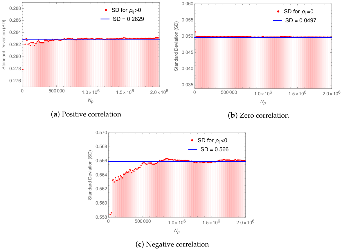
Example 2.

We consider a portfolio consisting of 20 assets evolving according to the MBS model introduced in Section 3.1. For each MC replication, the sample covariance matrix

$${\widehat{\mathit{C}}}_{N_p}^{\left(k\right)}$$

is computed using $N_p$ simulated trajectories, and the corresponding GMV portfolio weights are obtained through

$${\mathit{w}}_{\mathrm{MC}}^{\left(k\right)}={\displaystyle \frac{{\left({\widehat{\mathit{C}}}_{N_p}^{\left(k\right)}\right)}^{-1}\mathit{u}}{{\mathit{u}}^{\top }{\left({\widehat{\mathit{C}}}_{N_p}^{\left(k\right)}\right)}^{-1}\mathit{u}}}.$$

The resulting weights are compared with the benchmark GMV portfolio weights

$${\mathit{w}}_{\mathrm{CF}}={\displaystyle \frac{{\overline{\mathit{C}}}^{-1}\mathit{u}}{{\mathit{u}}^{\top }{\overline{\mathit{C}}}^{-1}\mathit{u}}},$$

where

$$\overline{\mathit{C}}$$

denotes the analytical covariance matrix derived in Section 3.2.

For each replication, we compute the Euclidean distance

$$\begin{array}{c}\hfill d_{N_p}^{\left(k\right)}={∥{\mathit{w}}_{\mathrm{CF}}-{\mathit{w}}_{\mathrm{MC}}^{\left(k\right)}∥}_2.\end{array}$$

(88)

The variability of this discrepancy measure is then summarized by its empirical standard deviation as a function of the number of MC trajectories $N_p$. The corresponding results are presented in Figure 3.

The results indicate that finite-sample variability in the GMV portfolio weights may remain noticeable even when a relatively large number of simulation paths is employed. This behavior reflects the sensitivity of the portfolio optimization procedure to perturbations in the covariance matrix, since the optimal weights depend explicitly on the inverse covariance matrix.

From a theoretical perspective, the consistency of the sample covariance matrix implies that the GMV portfolio weights constructed from the sample covariance matrix converge to their analytical counterparts as the number of observations tends to infinity, provided that the limiting covariance matrix is positive definite. Nevertheless, the numerical results demonstrate that this convergence may be sufficiently slow for finite samples to produce non-negligible differences in portfolio allocations.

Consequently, although the analytical covariance matrix and the sample covariance matrix yield asymptotically equivalent GMV portfolios, the analytical framework developed in this paper offers a useful benchmark for assessing the practical impact of covariance estimation errors in moderate-dimensional portfolio optimization problems.

5. Empirical Study

In this section, we investigate the practical applicability of the proposed portfolio optimization framework using historical stock price data from the $S\&P$ 500 index. Specifically, we estimate the parameters governing the MBS model with time-varying drift and volatility functions and subsequently employ these estimates to construct the closed-form covariance matrix derived in Corollary 1. The resulting covariance structure is then incorporated into the Markowitz mean–variance framework to generate the corresponding efficient frontier and examine the implications of the proposed model in a realistic financial setting.

The empirical analysis serves two purposes. First, it illustrates how the analytical results developed in Section 3.2, Section 3.3 and Section 3.4 can be implemented using observed market data. Second, it provides insights into the extent to which time-varying asset characteristics influence the covariance structure and the associated portfolio allocation decisions.

5.1. Data and Methodology

The empirical analysis aims to illustrate the practical implementation of the proposed portfolio optimization framework using real market data. To this end, we consider daily closing prices of 20 companies selected from the constituents of the $S\&P$ 500 index over the period from 2 January 2020 to 31 December 2024. The selected companies were drawn directly from the index constituents and were not chosen according to any specific portfolio construction criterion, such as sector classification, market capitalization, or correlation structure. The purpose of this empirical investigation is therefore not to identify an optimal investment universe but rather to demonstrate the applicability of the analytical framework developed in this paper.

Let $S_t^{\left(i\right)}$, $i=1,2,\dots ,20$, denote the price process of the i-th asset at time t. The asset price dynamics are assumed to follow the MBS model with time-varying parameters introduced in Section 3.1. In particular, the drift and volatility functions are specified according to Corollary 1 as

$$\begin{array}{cc}\hfill {\mu }_i\left(t\right)& ={\mu }_{i0}+{\mu }_{i1}t,\hfill \end{array}$$

(89)

$$\begin{array}{cc}\hfill {\sigma }_i\left(t\right)& ={\sigma }_{i0}+{\sigma }_{i1}t,\hfill \end{array}$$

(90)

for $i=1,\dots ,20$.

Prior to estimation, the raw price series are synchronized and screened for missing observations to ensure consistency across all assets. Daily logarithmic returns are subsequently computed from the cleaned price data and used for statistical inference.

The unknown parameters governing the time-varying drift and volatility functions are estimated using the maximum likelihood estimation approach. Since the proposed model is formulated as a continuous-time diffusion process observed at discrete time intervals, the exact likelihood function is generally unavailable in closed form. Consequently, we employ the asymptotic likelihood expansion methodology developed by Aït-Sahalia [22], which provides accurate approximations to the transition densities of discretely sampled diffusion processes. The resulting approximate likelihood functions are maximized numerically to obtain the parameter estimates together with their corresponding standard errors and confidence intervals.

The analytical covariance matrix derived in Corollary 1 additionally requires estimates of the pairwise correlation coefficients among the underlying Brownian motions. These coefficients are estimated using the empirical correlations of the observed daily logarithmic returns over the same sample period. The estimated correlations, together with the maximum likelihood estimates of the drift and volatility parameters, are subsequently incorporated into the closed-form covariance matrix developed in Section 3.2. This covariance structure then serves as the key input for the portfolio optimization framework considered in Section 3.3 and Section 3.4.

5.2. Empirical Study on 20 Assets from the $S\&P$ 500

Example 3.

We now present the estimation results for the parameters associated with the time-varying drift and volatility functions under the proposed MBS framework. The maximum likelihood estimates, together with their standard errors and corresponding 95% confidence intervals, are reported in

Table 1. Maximum Likelihood Estimates with Standard Errors and 95% Confidence Intervals for the Linear Drift and Volatility Parameters under the MBS Model.

Asset	Parameter	Estimate	SD Error	95% CI Lower	95% CI Upper
1	${\mu }_{10}$	0.3116	0.0598	0.1945	0.4288
	${\mu }_{11}$	−0.0091	0.1007	−0.2065	0.1883
	${\sigma }_{10}$	0.4290	0.0028	0.4236	0.4345
	${\sigma }_{11}$	−0.0497	0.0046	−0.0588	−0.0406
2	${\mu }_{20}$	0.3657	0.0350	0.2970	0.4344
	${\mu }_{21}$	−0.0931	0.0597	−0.2101	0.0239
	${\sigma }_{20}$	0.4401	0.0016	0.4370	0.4433
	${\sigma }_{21}$	−0.0201	0.0028	−0.0255	−0.0146
3	${\mu }_{30}$	0.1734	0.0250	0.1244	0.2224
	${\mu }_{31}$	0.0233	0.0437	−0.0624	0.1089
	${\sigma }_{30}$	0.4066	0.0011	0.4043	0.4088
	${\sigma }_{31}$	−0.0191	0.0020	−0.0230	−0.0152
4	${\mu }_{40}$	0.1341	0.0265	0.0821	0.1860
	${\mu }_{41}$	0.0115	0.0442	−0.0752	0.0982
	${\sigma }_{40}$	0.2923	0.0012	0.2899	0.2947
	${\sigma }_{41}$	−0.0349	0.0020	−0.0388	−0.0310
5	${\mu }_{50}$	−0.1612	0.0238	−0.2078	−0.1145
	${\mu }_{51}$	0.0633	0.0410	−0.0171	0.1437
	${\sigma }_{50}$	0.4420	0.0011	0.4398	0.4442
	${\sigma }_{51}$	−0.0443	0.0018	−0.0479	−0.0407
6	${\mu }_{60}$	0.2474	0.0166	0.2149	0.2798
	${\mu }_{61}$	0.0038	0.0289	−0.0529	0.0604
	${\sigma }_{60}$	0.3723	0.0008	0.3708	0.3738
	${\sigma }_{61}$	−0.0194	0.0014	−0.0221	−0.0167
7	${\mu }_{70}$	0.0953	0.0235	0.0494	0.1413
	${\mu }_{71}$	−0.0782	0.0410	−0.1586	0.0022
	${\sigma }_{70}$	0.4421	0.0011	0.4400	0.4442
	${\sigma }_{71}$	−0.0001	0.0019	−0.0038	0.0036
8	${\mu }_{80}$	0.1808	0.0155	0.1505	0.2110
	${\mu }_{81}$	−0.0543	0.0262	−0.1057	−0.0029
	${\sigma }_{80}$	0.2524	0.0007	0.2510	0.2538
	${\sigma }_{81}$	−0.0253	0.0012	−0.0276	−0.0230
9	${\mu }_{90}$	−0.0603	0.0180	−0.0955	−0.0251
	${\mu }_{91}$	0.0982	0.0306	0.0383	0.1581
	${\sigma }_{90}$	0.4260	0.0008	0.4244	0.4277
	${\sigma }_{91}$	−0.0483	0.0014	−0.0510	−0.0456
10	${\mu }_{100}$	0.0680	0.0244	0.0202	0.1158
	${\mu }_{101}$	0.0359	0.0396	−0.0417	0.1135
	${\sigma }_{100}$	0.4481	0.0011	0.4460	0.4502
	${\sigma }_{101}$	−0.0655	0.0018	−0.0691	−0.0620
11	${\mu }_{110}$	0.0201	0.0249	−0.0287	0.0689
	${\mu }_{111}$	0.1160	0.0427	0.0324	0.1996
	${\sigma }_{110}$	0.5338	0.0012	0.5315	0.5361
	${\sigma }_{111}$	−0.0323	0.0025	−0.0372	−0.0274
12	${\mu }_{120}$	0.3755	0.0146	0.3469	0.4041
	${\mu }_{121}$	−0.0510	0.0248	−0.0996	−0.0024
	${\sigma }_{120}$	0.4099	0.0007	0.4086	0.4112
	${\sigma }_{121}$	−0.0456	0.0019	−0.0493	−0.0419
13	${\mu }_{130}$	−0.0318	0.0327	−0.0959	0.0324
	${\mu }_{131}$	0.1347	0.0556	0.0258	0.2436
	${\sigma }_{130}$	0.6280	0.0015	0.6252	0.6309
	${\sigma }_{131}$	−0.0641	0.0025	−0.0689	−0.0593
14	${\mu }_{140}$	0.6539	0.0240	0.6068	0.7010
	${\mu }_{141}$	0.0453	0.0424	−0.0378	0.1284
	${\sigma }_{140}$	0.5774	0.0011	0.5752	0.5796
	${\sigma }_{141}$	−0.0173	0.0019	−0.0211	−0.0135
15	${\mu }_{150}$	0.1327	0.0148	0.1036	0.1617
	${\mu }_{151}$	−0.0101	0.0252	−0.0596	0.0393
	${\sigma }_{150}$	0.2754	0.0006	0.2741	0.2766
	${\sigma }_{151}$	−0.0301	0.0011	−0.0323	−0.0279
16	${\mu }_{160}$	−0.0095	0.0284	−0.0651	0.0461
	${\mu }_{161}$	0.0192	0.0483	−0.0754	0.1138
	${\sigma }_{160}$	0.5757	0.0012	0.5732	0.5781
	${\sigma }_{161}$	−0.0511	0.0020	−0.0550	−0.0472
17	${\mu }_{170}$	1.2582	0.0398	1.1801	1.3362
	${\mu }_{171}$	−0.2060	0.0685	−0.3403	−0.0718
	${\sigma }_{170}$	0.7851	0.0018	0.7816	0.7886
	${\sigma }_{171}$	−0.0491	0.0031	−0.0552	−0.0430
18	${\mu }_{180}$	0.3768	0.0187	0.3401	0.4135
	${\mu }_{181}$	−0.0833	0.0317	−0.1455	−0.0211
	${\sigma }_{180}$	0.3676	0.0008	0.3660	0.3692
	${\sigma }_{181}$	−0.0309	0.0014	−0.0337	−0.0281
19	${\mu }_{190}$	0.0170	0.0111	−0.0047	0.0387
	${\mu }_{191}$	0.0494	0.0185	0.0131	0.0858
	${\sigma }_{190}$	0.3862	0.0005	0.3853	0.3872
	${\sigma }_{191}$	−0.0501	0.0008	−0.0517	−0.0485
20	${\mu }_{200}$	−0.0541	0.0151	−0.0837	−0.0245
	${\mu }_{201}$	0.1026	0.0258	0.0521	0.1531
	${\sigma }_{200}$	0.2855	0.0007	0.2842	0.2869
	${\sigma }_{201}$	−0.0259	0.0012	−0.0282	−0.0236

.

The estimated intercept parameters associated with the drift functions exhibit substantial variation across assets, reflecting the heterogeneous growth characteristics of the selected stocks. Some assets display relatively large positive drift estimates, whereas others exhibit smaller or even negative values. By contrast, the slope parameters governing the time dependence of the drift functions are generally small in magnitude. For many assets, the corresponding confidence intervals include zero, suggesting that the empirical evidence supporting time-varying drift is relatively weak over the sample period considered.

The volatility estimates reveal a different pattern. The intercept parameters are uniformly positive and lie within ranges commonly observed in equity markets. Moreover, a considerable proportion of the volatility slope parameters are negative and statistically significant, indicating a tendency toward declining volatility over the sample period for several assets. These findings suggest that allowing for time-varying volatility may provide a more flexible and realistic description of asset price dynamics than the conventional constant-volatility assumption.

The estimated parameters are subsequently incorporated into the analytical covariance matrix derived in Corollary 1. This covariance structure is then employed within the Markowitz framework to construct the corresponding efficient frontier implied by the proposed model. For comparison purposes, we also consider the efficient frontier obtained using the conventional sample covariance matrix estimated directly from historical returns.

Overall, the empirical findings demonstrate that the proposed time-varying specification provides a flexible mechanism for capturing heterogeneous behaviors in drift and volatility across multiple assets. More importantly, the results illustrate how the analytical covariance matrix developed in this paper can be calibrated using observed market data and subsequently incorporated into the portfolio optimization framework. This highlights the practical applicability of the proposed model-driven approach to mean–variance portfolio selection.

Following the construction of the analytical covariance matrix, Figure 4 presents the resulting efficient frontiers under parameter uncertainty. The model-implied frontier is generated using the closed-form covariance matrix developed in this paper, whereas the empirical frontier is based on the traditional sample covariance estimator.

Several observations emerge from the figure. First, the model-implied efficient frontier exhibits a shape similar to that of the empirical frontier, suggesting that the proposed framework is capable of capturing the overall risk–return characteristics observed in the market. However, noticeable differences between the two frontiers remain, particularly in regions corresponding to higher expected returns. This indicates that the choice of covariance estimation methodology can substantially influence the portfolio allocations identified as efficient.

Second, the analytical covariance matrix leads to a smoother efficient frontier, reflecting the model-driven nature of the proposed approach. In contrast, the empirical frontier constructed from the sample covariance matrix is more susceptible to sampling variability arising from finite historical observations. This observation is consistent with the finite-sample sensitivity discussed in Section 4.

Finally, the upper and lower 95% confidence bands provide insights into the impact of parameter uncertainty on portfolio optimization. The widening of these bands as the expected portfolio return increases suggests that portfolios targeting more aggressive return levels are associated with greater uncertainty in the corresponding risk estimates. Consequently, investors seeking higher expected returns may face a larger degree of estimation risk, emphasizing the importance of accounting for parameter uncertainty when constructing efficient portfolios.

The confidence bands are obtained by constructing the analytical covariance matrix using the lower and upper 95% confidence limits of the estimated model parameters reported in Table 1. The resulting efficient frontiers therefore provide a sensitivity analysis of the portfolio risk–return relationship with respect to parameter estimation uncertainty. Although this approach illustrates the impact of estimation uncertainty on portfolio construction, it does not explicitly incorporate parameter uncertainty into the portfolio optimization problem itself.

Overall, Figure 4 demonstrates that the proposed analytical covariance framework not only provides a tractable alternative to conventional sample covariance estimation but also yields portfolio risk–return relationships that remain consistent with empirical market behavior. These findings highlight the practical applicability of the proposed methodology in mean–variance portfolio selection under time-varying market conditions.

In the empirical analysis considered in this study, the analytical covariance matrix constructed from the estimated model parameters remained positive definite, allowing the efficient frontier and optimal portfolios to be computed successfully. Nevertheless, in higher-dimensional applications or under different market conditions, parameter estimation may produce covariance matrices that are close to singular. Investigating numerical stability and appropriate regularization techniques in such settings constitutes an interesting direction for future research.

6. Limitations and Future Research Directions

The analytical framework developed in this paper provides a model-driven approach to covariance matrix construction and portfolio optimization under an MBS model with time-varying parameters. By deriving the covariance matrix analytically from the underlying stochastic asset-price model, the proposed methodology establishes a direct connection between continuous-time asset pricing theory and the classical Markowitz mean–variance framework. Nevertheless, as with any analytical model, the present study is subject to several assumptions and limitations that naturally suggest directions for future research.

• Model dependence of the analytical covariance matrix.
  The closed-form covariance matrix derived in this paper is specific to the MBS model with deterministic time-varying drift and volatility functions. Consequently, its validity depends on the adequacy of the underlying diffusion model in describing the dynamics of asset prices. In situations where market behaviour exhibits stochastic volatility, jump components, rough volatility, or regime-switching effects, the analytical covariance representation developed herein may no longer be directly applicable. Extending the present framework to more general stochastic asset-price models therefore represents an important avenue for future research.
• Simplifying assumptions on model parameters.
  For empirical implementation, the drift and volatility functions are assumed to evolve linearly over time, while the instantaneous correlation matrix is assumed to remain constant throughout the investment horizon. These assumptions are adopted to preserve analytical tractability and enable explicit closed-form expressions. Although they provide a useful first approximation to slowly evolving market conditions, they may not adequately capture nonlinear parameter dynamics, time-varying correlations, or abrupt structural changes frequently observed in financial markets. Future research may therefore consider more flexible deterministic parameterizations or stochastic specifications for both volatilities and correlations.
• Parameter estimation uncertainty.
  The proposed covariance matrix is obtained analytically once the model parameters have been estimated from historical data. Consequently, estimation errors in the drift, volatility, and correlation parameters inevitably propagate into the resulting covariance matrix and the corresponding optimal portfolio allocations. Although confidence intervals for the estimated parameters are reported and their effects on the efficient frontier are partially illustrated, a comprehensive theoretical investigation of parameter uncertainty remains beyond the scope of the present study. Future work may consider asymptotic sensitivity analysis, bootstrap methods, Bayesian inference, or robust portfolio optimization to quantify the impact of estimation uncertainty more systematically.
• Relationship with modern covariance estimation methods.
  The empirical analysis compares the proposed analytical covariance matrix with the conventional sample covariance matrix, which serves as the classical benchmark in the original Markowitz framework. The objective of this comparison is to illustrate the implementation and characteristics of the proposed model-driven methodology rather than establish empirical superiority over existing statistical covariance estimation techniques. In contemporary portfolio management, numerous alternative estimators have been developed, including shrinkage estimators, factor-model covariance matrices, exponentially weighted covariance estimators, random matrix filtering, Bayesian approaches, and multivariate GARCH or dynamic conditional correlation models. A systematic comparison between the proposed model-implied covariance matrix and these modern covariance estimation approaches would provide valuable additional insight and constitutes an important direction for future investigation.
• Empirical validation and portfolio performance evaluation.
  The empirical study is designed primarily to demonstrate the practical implementation and feasibility of the proposed analytical framework using real financial data. While the resulting efficient frontiers illustrate the influence of the model-implied covariance matrix on portfolio construction, the present work does not include a comprehensive out-of-sample portfolio evaluation based on rolling-window estimation or dynamic portfolio rebalancing. Consequently, practical investment performance measures such as realised portfolio volatility, Sharpe ratio, maximum drawdown, portfolio turnover, and transaction-cost-adjusted returns are not examined. Incorporating these performance metrics would provide a more complete assessment of the proposed methodology from an investment management perspective.
• Generality of the empirical investigation.
  The empirical analysis is conducted using twenty constituent stocks of the S&P 500 index over the period 2020–2024. The purpose of this empirical study is to illustrate the applicability of the proposed analytical framework rather than establish universal empirical conclusions across different markets, asset classes, or investment horizons. Future investigations may consider larger investment universes, international equity markets, fixed-income securities, commodities, cryptocurrencies, and other financial assets in order to further evaluate the robustness and practical applicability of the proposed methodology under diverse market environments.

Overall, these limitations do not diminish the theoretical contribution of the present study. Rather, they define the scope of the proposed analytical framework and identify several promising directions through which the methodology may be extended to accommodate more realistic market dynamics, broader classes of stochastic asset-price models, and more comprehensive empirical portfolio evaluation.

7. Conclusions

In this paper, we have developed a model-driven analytical framework for portfolio optimization under an MBS model with time-varying parameters. By allowing both the drift and volatility functions to evolve linearly over time, we derived explicit closed-form expressions for the covariance matrix of normalized asset prices. This analytical covariance representation establishes a direct connection between continuous-time stochastic asset-price modeling and the classical Markowitz mean–variance portfolio optimization framework.

Building upon the analytical covariance matrix, we obtained explicit closed-form representations for the global minimum-variance portfolio, the mean–variance efficient portfolio, and the corresponding efficient frontier. Unlike conventional implementations of the Markowitz model that rely exclusively on covariance matrices estimated from historical return data, the proposed methodology constructs the covariance matrix directly from the underlying stochastic asset-price model once the model parameters have been specified or estimated. This provides a mathematically consistent framework for integrating continuous-time asset pricing models with analytical portfolio optimization.

The numerical experiments demonstrated the finite-sample sensitivity of portfolio optimization with respect to covariance estimation. Although the conventional sample covariance matrix remains a consistent estimator under the assumed model, the resulting portfolio allocations may exhibit substantial variability due to the nonlinear dependence of optimal portfolio weights on the inverse covariance matrix. These findings illustrate the importance of stable covariance structures in practical mean–variance portfolio construction.

To illustrate the practical applicability of the proposed methodology, we conducted an empirical study using daily stock price data from twenty constituents of the S&P 500 index over the period 2020–2024. The parameters of the MBS model with time-varying coefficients were estimated using the maximum likelihood framework of Aït-Sahalia [22]. The empirical results demonstrate how the estimated model parameters can be incorporated into the analytical covariance matrix for constructing efficient frontiers under realistic market conditions, thereby illustrating the feasibility of the proposed framework in practical financial applications.

Overall, the proposed methodology provides an analytically tractable framework that links stochastic asset-price models with portfolio optimization through explicit covariance representations. Rather than replacing existing statistical covariance estimation techniques, the proposed framework offers a complementary model-based approach that is fully consistent with the assumed stochastic dynamics of asset prices while preserving analytical tractability. We believe that the methodology developed in this paper provides a useful foundation for further research on analytical covariance representations and their applications to portfolio optimization under more general stochastic financial models.