A Predefined-Time Neurodynamic Approach for Solving Generalized Absolute Value Equations

Abstract

This paper proposes a predefined-time stable neurodynamic approach for solving generalized absolute value equations. In contrast to conventional fixed-time stability methods, the proposed approach provides greater flexibility and broader applicability through the inclusion of an adjustable time parameter. Under appropriate conditions, the method is rigorously proven to converge to the unique solution within a predefined time frame. Finally, numerical simulations are conducted to validate the convergence performance of the proposed neurodynamic method.

1. Introduction

It is well-known that generalized absolute value equations (GAVEs) and absolute value equations (AVEs) play a very important role in the fields of mathematical optimization and engineering applications, such as linear complementarity problems [1], variational inequalities [2], physical contact of mechanical structures [3], network prices [4], linear interval equations [5] and cancellable biometric systems [6]. Many scholars study solving GAVEs; see [7,8]. In this paper, we consider the following GAVEs:

$$Ax-B\left|x\right|=c,$$

(1)

where $A,B\in {\mathbb{R}}^{m\times n}$ and $c\in {\mathbb{R}}^m$ are known, $x\in {\mathbb{R}}^n$ is the unknown vector, and $\left|x\right|=\left[\right|x_1|,|x_2|,\cdots ,|x_n{\left|\right]}^T$. Specially, when B is the identity matrix, (1) degenerates to the following AVEs:

$$Ax-\left|x\right|=c,$$

where $A\in {\mathbb{R}}^{n\times n}$ is invertible, $c\in {\mathbb{R}}^n$ and $x\in {\mathbb{R}}^n$. It can be observed that GAVEs extend the concept of AVEs, while AVEs are a special case of this generalized form. Solving GAVEs is known to be NP-hard [9]. Despite this inherent difficulty, GAVEs possess a relatively simple structure and are closely related to numerous optimization problems. As a result, solving such equations has drawn substantial research interest, as seen in works such as [10].

Research in neurodynamic approaches was pioneered in the mid-1980s by Hopfield and Tank [11], and has been widely applied in many fields, including scientific computing [12], financial engineering [13], feedback control [14], and multiobjective optimization [15]. Neurodynamic approaches have recently been extended to address both optimization problems and GAVEs. Neurodynamic approaches to GAVEs are built upon the equivalence between the solutions to these equations and the equilibrium points of their associated dynamical systems, implying that solving the former is reduced to computing the latter.

Finite-time stability, originally proposed by [16], has been adopted to accelerate the convergence of certain recurrent neural networks. Subsequently, to eliminate the dependence of the settling time on initial conditions, ref. [17] introduced the concept of fixed-time stability. Some scholars have conducted research using this concept. For example, ref. [18] propose a finite-time converging proximal dynamic model to deal with equilibrium problems. Neither infinite-time nor fixed-time methods allow the user to directly prescribe the desired convergence time upper bound, making it difficult to achieve task-specific deadlines. The concept of predefined-time stability was introduced by [19]. In this framework, the stability time is independent of initial values and varies with user-defined parameters. By adjusting these parameters, users can control the system’s stabilization time, providing greater autonomy and enabling independent adjustment. In contrast, in real-time engineering systems such as autonomous collision avoidance, robotic manipulator synchronization, and networked control systems, where strict deterministic time constraints are imposed, predefined-time stability becomes particularly critical. For further reference, research on related neurodynamic approaches can be found in the following works: fixed-time methods in [20,21], finite-time optimization approaches in [22,23], predefined-time strategies in [24,25], and inverse-free formulations in [26]. Finite-time and fixed-time analyses focus solely on proving convergence within a finite or fixed horizon. Predefined-time analysis, on the other hand, allows users to specify the convergence time upper bound beforehand and actively utilizes this information during control execution. Consequently, the latter offers greater design flexibility. Some authors have conducted research on predefined-time stability. A novel theorem focusing on predefined-time stability within fractional-order systems was introduced in [27]. Predefined-time inverse-free neurodynamic approaches for solving AVEs are proposed in [28]. Ref. [29] proposed a novel neurodynamic approach with predefined-time stability for mixed variational inequality problems.

Although predefined-time approaches have been widely adopted for diverse optimization problems, their application to GAVEs remains unexplored. Moreover, the existing finite-time and fixed-time approaches for solving GAVEs yield convergence time bounds that cannot be preset by users, which restricts their practical applicability in engineering systems. Motivated by these insights, we propose a predefined-time stable dynamical system for solving GAVEs. Under given conditions, the approach converges to a unique solution within user-defined time. And robustness against perturbations is rigorously analyzed. The main contributions of this paper are summarized as follows.

• Previous research has predominantly addressed AVEs, such as [30]. In contrast, this paper significantly extends the scope by systematically investigating GAVEs, thereby contributing a more comprehensive and applicable theoretical and computational framework to the field.
• This paper makes a distinct contribution by advancing beyond the conventional frameworks of finite-time and fixed-time stability to introduce a predefined-time stable dynamic system for solving GAVEs. Unlike existing approaches, the proposed system allows the upper bound of the convergence time to be explicitly pre-specified by the user, independent of the initial system state, thereby offering enhanced predictability and practicality for real-time applications.
• A key contribution of this work is that the proposed neurodynamic approach does not require explicit matrix inversion, which is a common limitation in many existing methods. While approaches such as the modified Newton-type iteration in [8] can solve GAVEs, they inherently depend on the matrix being invertible. In contrast, the proposed neurodynamic approach operates without any matrix inversion, substantially broadening its applicability to problems where the system matrix is singular or ill-conditioned.

This paper is organized as follows. In Section 2, some fundamental definitions and concepts are reviewed. In Section 3, a predefined-time stable dynamic system is proposed and employed to solve GAVEs. Furthermore, the stability was analytically investigated. In Section 4, numerical simulations are presented to verify the theoretical results.

Notations: Throughout this paper, without special statements, let $\mathbb{R}$ denotes the set of real numbers and I denote the identity matrix. For $A\in {\mathbb{R}}^{n\times n}$, the symbol $A^T$ denotes its transpose. Its norm $\parallel A\parallel$ is defined by $\parallel A\parallel :=\max \left\{\parallel Ax\parallel :x\in {\mathbb{R}}^n,\parallel x\parallel =1\right\}$. The smallest singular value of A is denoted by ${\sigma }_{\min }\left(A\right)$. For two vectors $x,y\in {\mathbb{R}}^n$, their inner product is defined as $x^{T}y={\sum }_{i=1}^n{x}_i{y}_i$, and the 2-norm of x is given by $\parallel x\parallel =\sqrt{x^{T}x}$.

2. Preliminaries

In this section, we introduce some fundamental properties of GAVEs and dynamical systems, in order to establish their connections and lay the groundwork for the analysis that follows. Next, we briefly recall some important results about the GAVEs (1).

Lemma 1

([31]). Suppose that $A,B\in {\mathbb{R}}^{n\times n}$ and ${\sigma }_{\min }\left(A\right)>\parallel B\parallel$. Then (1) has a unique solution for any $c\in {\mathbb{R}}^n$.

Lemma 2

([32]). Let $A,B\in {\mathbb{R}}^{n\times n}$ and $c\in {\mathbb{R}}^n$. If $x^{\ast }$ is the unique solution to (1) and ${\sigma }_{\min }\left(A\right)>\parallel B\parallel$, then for any $x\in {\mathbb{R}}^n$, we can get that

$${(x-x^{\ast })}^T{A}^T(Ax-B|x|-c)\ge {\displaystyle \frac{1}{2}}{\parallel Ax-B\left|x\right|-c\parallel }^2$$

(2)

and

$${\displaystyle \frac{1}{\parallel A\parallel +\parallel B\parallel }}\parallel Ax-B\left|x\right|-c\parallel \le \parallel x-x^{\ast }\parallel \le {\displaystyle \frac{1}{{\sigma }_{\min }\left(A\right)-\parallel B\parallel }}\parallel Ax-B\left|x\right|-c\parallel .$$

(3)

Definition 1

([33]). Let $f:{\mathbb{R}}^n\to {\mathbb{R}}^n$ be a continuous function. Consider the following system:

$${\displaystyle \frac{dx}{dt}}=f\left(x\left(t\right)\right),x\left(0\right)=x_0\in {\mathbb{R}}^n.$$

(4)

A point $x^{\ast }\in {\mathbb{R}}^n$ is said to be an equilibrium point of (4) if $f\left(x^{\ast }\right)=\mathbf{0}$.

We state some definitions related to the convergence of system (4).

Definition 2

([16,17]). Consider the system (4), and the equilibrium point of (4) is called:

(i)  Finite-time stability. The equilibrium point of (4) is deemed globally finite-time stable if it is globally asymptotically stability and if any solution $x\left(t\right)$ of (4) with initial point $x\left(0\right)$ reaches the equilibrium within a finite-time; i.e., $\forall t\ge T\left(x\right(0\left)\right):x\left(t\right)=0$, where $T:{\mathbb{R}}^n\to \mathbb{R}\cup \{+\infty \}$ represents the settling-time function.

(ii) Fixed-time stability. The equilibrium point of (4) is fixed-time stable if it is globally finite-time stable and the settling-time function is bounded; i.e., $\exists T_{\max }>0:\forall x\left(0\right)\in {\mathbb{R}}^n$, $T\left(x\left(0\right)\right)\le T_{\max }$.

(iii) Predefined-time stability. If the parameter $T_c>0$ can be adjusted to predict the settling time $T\left(x\right(0\left)\right)$ for achieving fixed-time stability, it implies that the driving response system (4) can attain global predefined-time stability, where $T\left(x\left(0\right)\right)\le T_c$.

Lemma 3

([34]). Suppose $V:{\mathbb{R}}^n\to \mathbb{R}$ is a continuous, non-negative and unbounded radial function satisfying the following inequality:

$$\dot{V}\left(x\left(t\right)\right)\le -(c_1{V}^{{\kappa }_1}\left(x\left(t\right)\right)+c_2{V}^{{\kappa }_2}\left(x\left(t\right)\right)+c_{3}V\left(x\left(t\right)\right)),\forall x\left(t\right)\in {\mathbb{R}}^n\setminus \left\{\mathbf{0}\right\},$$

(5)

where $c_1,c_2,c_3>0,{\kappa }_1\in (0,1)$ and ${\kappa }_2>1$. Then, the system (4) achieves convergence within a fixed-time, where

$$T_{\max }={\displaystyle \frac{1}{c_3(1-{\kappa }_1)}}\ln (1+{\displaystyle \frac{c_3}{c_1}})+{\displaystyle \frac{1}{c_3({\kappa }_2-1)}}\ln (1+{\displaystyle \frac{c_3}{c_2}}).$$

Lemma 4

([29]). Consider the system (4). If there exists a positive definite unbounded radial function $V:{\mathbb{R}}^n\to \mathbb{R}$ and $T_c$ is a user-defined parameter satisfying the following conditions,

(i) $V\left(x\left(t\right)\right)=0\iff \dot{x}\left(t\right)=0$;

(ii) For any $V\left(x\right(t\left)\right)>0$, there exists $c_1,c_2,c_3,{\kappa }_1,{\kappa }_2,T_c,G_c>0$, where ${\kappa }_2>1$ and $0<{\kappa }_1<1$, such that the following inequality holds:

$$\dot{V}\left(x\left(t\right)\right)\le -{\displaystyle \frac{G_c}{T_c}}(c_1{V}^{{\kappa }_1}\left(x\left(t\right)\right)+c_2{V}^{{\kappa }_2}\left(x\left(t\right)\right)+c_{3}V\left(x\left(t\right)\right)),$$

then the system (4) achieves fixed-time stability within the predefined time $T_c$, where

$$G_c={\displaystyle \frac{1}{c_3(1-{\kappa }_1)}}\ln (1+{\displaystyle \frac{c_3}{c_1}})+{\displaystyle \frac{1}{c_3({\kappa }_2-1)}}\ln (1+{\displaystyle \frac{c_3}{c_2}}).$$

3. A Neurodynamic Approach and Its Analysis

This section proposes a predefined-time stable dynamic system for solving problem (1), provides an explicit upper bound for the convergence time, and demonstrates its robustness against disturbances.

3.1. The Predefined-Time Stable Neurodynamic Approach

This section presents a predefined-time stable dynamic system for solving the GAVEs (1).

$${\displaystyle \frac{dx}{dt}}=-{\displaystyle \frac{G_c}{T_c}}\rho \left(x\right)g(\gamma ,x),$$

(6)

where

$$\rho \left(x\right)=\left\{\begin{array}{cc}{\displaystyle \frac{{\rho }_1}{{\Vert \mathsf{\Phi }\left(x\right)\Vert }^{1-{\lambda }_1}}}+{\displaystyle \frac{{\rho }_2}{{\Vert \mathsf{\Phi }\left(x\right)\Vert }^{1-{\lambda }_2}}}+{\rho }_3,\hfill & \mathrm{if}\mathsf{\Phi }\left(x\right)\ne \mathbf{0},\hfill \\ 0,\hfill & \mathrm{if}\mathsf{\Phi }\left(x\right)=\mathbf{0},\hfill \end{array}\right.$$

and $\mathsf{\Phi }\left(x\right)=Ax-B\left|x\right|-c$, $g(\gamma ,x)=\gamma A^T\mathsf{\Phi }\left(x\right)$, ${\rho }_1,{\rho }_2,{\rho }_3,\gamma ,T_c,G_c>0$, ${\lambda }_1\in (0,1)$ and ${\lambda }_2\in (1,+\infty )$.

Algorithmically, for a given initial point $x\left(0\right)$, the state $x\left(t\right)$ evolves according to the differential Equation (6). At each integration step, the residual $\mathsf{\Phi }\left(x_k\right)$ is computed from the current state; if $\mathsf{\Phi }\left(x_k\right)\ne \mathbf{0}$, the gain $\rho \left(x_k\right)$ is evaluated and the state is updated using the forward-Euler discretization

$$x_{k+1}=x_k-h·{\displaystyle \frac{G_c}{T_c}}·\rho \left(x_k\right)·g(\gamma ,x_k).$$

The iteration terminates when the prescribed time $T_c$ is reached (up to the discretization step), or the change between successive iterates falls below a tolerance $\epsilon$, or a maximum iteration count $K_{\max }$ is exceeded. The final state $x_k$ is then taken as the approximate solution to the GAVE. The complete numerical implementation is summarized in Algorithm 1.

Algorithm 1 Forward-Euler discretization of approach (7).

1: Input:   2:    Initial state: $x_0$; time step: $h>0$; parameters: $T_c>0$, $G_c>0$, $\gamma >0$, ${\rho }_1>0$, ${\rho }_2>0$, ${\rho }_3>0$; exponents: ${\lambda }_1\in (0,1)$, ${\lambda }_2\in (1,\infty )$; matrices: A, B; vector: c;   3:     tolerance: $\epsilon >0$; maximum iterations: $K_{\max }$   4: Output: State sequence ${\left\{x_i\right\}}_{i=0}^k$, where $k\le K_{\max }$ is the actual stopping step   5: Initialize: $x\leftarrow x_0$; $k\leftarrow 0$   6: while $k<K_{\max }$ do   7:       Compute $\mathsf{\Phi }\leftarrow Ax-B\left|x\right|-c$   8:       if $\parallel \mathsf{\Phi }\parallel =0$ then   9:            $\rho \leftarrow 0$ 10:       else 11:            $\rho \leftarrow {\displaystyle \frac{{\rho }_1}{{\parallel \mathsf{\Phi }\parallel }^{1-{\lambda }_1}}}+{\displaystyle \frac{{\rho }_2}{{\parallel \mathsf{\Phi }\parallel }^{1-{\lambda }_2}}}+{\rho }_3$ 12:       end if 13:       Compute $g\leftarrow \gamma A^T\mathsf{\Phi }$ 14:       Compute $x_{\mathrm{new}}\leftarrow x-h·{\displaystyle \frac{G_c}{T_c}}·\rho ·g$ 15:       if $\parallel x_{\mathrm{new}}{-x\parallel }_{\infty }<\epsilon$ then 16:            $x_{k+1}\leftarrow x_{\mathrm{new}}$ 17:            break 18:       end if 19:       $x_{k+1}\leftarrow x_{\mathrm{new}}$ 20:       $x\leftarrow x_{\mathrm{new}}$ 21:       $k\leftarrow k+1$ 22: end while 23: return ${\left\{x_i\right\}}_{i=0}^k$

From the perspective of collaborative design in control and optimization, this neurodynamic approach (6) can be comprehensively interpreted as follows: for the nonsmooth optimization problem represented by the generalized absolute value equation, the algorithm constructs a dynamic system with predefined-time convergence and a dual-power time-varying gain mechanism, where the gain function $\rho \left(x\right)$ regulates the convergence behavior near and far from the equilibrium point through the power terms ${\lambda }_1\in (0,1)$ and ${\lambda }_2\in (1,\infty )$, respectively, combined with a constant positive term ${\rho }_3$ to ensure terminal attractiveness. The driving term employs the simplified gradient direction $\gamma A^T\mathsf{\Phi }\left(x\right)$ in place of the conventional nonsmooth gradient, effectively circumventing the direct differentiation challenge of the absolute value term. This design essentially achieves a deep integration of gain adaptive scheduling from control theory and gradient flow modification from optimization theory. By real-time compensation of the inexact gradient direction via the gain term $G_c/T_c·\rho \left(x\right)$, the system state converges to the solution set within the predefined time $T_c$, while simultaneously exhibiting robustness against parameter perturbations and computational errors.

From Lemma 1, we obtain the following result on the existence and uniqueness of the solution trajectory for the system (6).

Proposition 1.

Suppose that $A,B\in {\mathbb{R}}^{n\times n}$ and ${\sigma }_{\min }\left(A\right)>\parallel B\parallel$. Then the system (6) has a unique equilibrium point $x^{\ast }$ for any $c\in {\mathbb{R}}^n$. Furthermore, $x^{\ast }$ is the unique solution of (1).

Proof. 

Suppose $x^{\ast }$ is an equilibrium point of system (6), then

$$-{\displaystyle \frac{G_c}{T_c}}\rho \left(x^{\ast }\right)\gamma A^T\mathsf{\Phi }\left(x^{\ast }\right)=\mathbf{0}.$$

It follows from $T_c,G_c,\gamma >0$ that

$$\rho \left(x^{\ast }\right)A^T\mathsf{\Phi }\left(x^{\ast }\right)=\mathbf{0}.$$

Since ${\sigma }_{\min }\left(A\right)>\parallel B\parallel$, then A is invertible. Together with system (6), this implies that

$$\mathsf{\Phi }\left(x^{\ast }\right)=\mathbf{0}.$$

So $x^{\ast }$ is a solution of (1). For any $c\in {\mathbb{R}}^n$, it follows from the condition ${\sigma }_{\min }\left(A\right)>\left|B\right|$ and Lemma 1 that $x^{\ast }$ is a unique solution of (1).

Conversely, assuming that $x^{\ast }$ is a solution of (1), then $\mathsf{\Phi }\left(x^{\ast }\right)=\mathbf{0}$. Furthermore,

$$-{\displaystyle \frac{G_c}{T_c}}\rho \left(x^{\ast }\right)\gamma A^T\mathsf{\Phi }\left(x^{\ast }\right)=\mathbf{0}.$$

This implies that $x^{\ast }$ is a equilibrium point of system (6). This completes the proof. □

Remark 1.

We provide the following instructions for the system (6).

(i) 

It follows from Definition 1 that if a point $x^{\ast }\in {\mathbb{R}}^n$ satisfies $\mathsf{\Phi }\left(x^{\ast }\right)=A{x}^{\ast }-B\left|x^{\ast }\right|-c=\mathbf{0}$, then $x^{\ast }$ is an equilibrium point of (6).

(ii) 

It follows from the definition of $\mathsf{\Phi }\left(x\right)$, if $\parallel \mathsf{\Phi }\parallel$ is large, it implies far from equilibrium points of (6); if $\parallel \mathsf{\Phi }\parallel$ is small, it implies close to equilibrium points.

(iii) 

The function $\rho \left(x\right)$ is designed with a three-term structure to cover all convergence stages. If $\mathsf{\Phi }\left(x\right)\ne \mathbf{0}$, then $\rho \left(x\right)>{\rho }_3$. Thus, ${\rho }_3$ ensures a strictly positive lower bound $\rho \left(x\right)\ge {\rho }_3>0$ for all $\mathsf{\Phi }\left(x\right)\ne \mathbf{0}$. This prevents numerical singularities and convergence stagnation, serving two key purposes: it provides a minimum convergence speed guarantee, and it avoids system stagnation in intermediate regions.

(iv) 

If $\parallel \mathsf{\Phi }\left(x\right)\parallel \to 0$, since ${\lambda }_1\in (0,1)$ and ${\lambda }_2>1$, then ${\displaystyle \frac{{\rho }_1}{{\parallel \mathsf{\Phi }\left(x\right)\parallel }^{1-{\lambda }_1}}}\to \infty$ and ${\displaystyle \frac{{\rho }_2}{{\parallel \mathsf{\Phi }\left(x\right)\parallel }^{1-{\lambda }_2}}}\to 0$. This implies that when close to equilibrium, ${\displaystyle \frac{{\rho }_1}{{\Vert \mathsf{\Phi }\left(x\right)\Vert }^{1-{\lambda }_1}}}$ is large and ${\displaystyle \frac{{\rho }_2}{{\Vert \mathsf{\Phi }\left(x\right)\Vert }^{1-{\lambda }_2}}}$ is small. In this case, the term ${\displaystyle \frac{{\rho }_1}{{\Vert \mathsf{\Phi }\left(x\right)\Vert }^{1-{\lambda }_1}}}$ becomes the dominant factor, which ensures finite-time convergence.

(v) 

If far from equilibrium, since ${\lambda }_1\in (0,1)$ and ${\lambda }_2>1$, then ${\displaystyle \frac{{\rho }_1}{{\Vert \mathsf{\Phi }\left(x\right)\Vert }^{1-{\lambda }_1}}}\to 0$ and ${\displaystyle \frac{{\rho }_2}{{\Vert \mathsf{\Phi }\left(x\right)\Vert }^{1-{\lambda }_2}}}\to \infty$. This implies that away from equilibrium, ${\displaystyle \frac{{\rho }_1}{{\Vert \mathsf{\Phi }\left(x\right)\Vert }^{1-{\lambda }_1}}}$ becomes small while ${\displaystyle \frac{{\rho }_2}{{\Vert \mathsf{\Phi }\left(x\right)\Vert }^{1-{\lambda }_2}}}$ becomes large. In this case, the term ${\displaystyle \frac{{\rho }_2}{{\Vert \mathsf{\Phi }\left(x\right)\Vert }^{1-{\lambda }_2}}}$ dominates and provides a strong driving force, enabling rapid convergence toward the equilibrium region.

(vi) 

If far from equilibrium and ${\lambda }_2\le 1$, then $1-{\lambda }_2\ge 0$, and the denominator ${\parallel \mathsf{\Phi }\parallel }^{1-{\lambda }_2}$ would not tend to zero as $\parallel \mathsf{\Phi }\parallel \to \infty$; in fact, it would remain bounded from below (when ${\lambda }_2=1$) or grow without bound (when ${\lambda }_2<1$). Consequently, the second gain term would be bounded or even decay to zero, failing to provide a sufficiently strong driving force for large initial errors.

(vii) 

The predefined-time stable dynamic system (6) can be equivalently reformulated as follows:

$$\begin{array}{ccc}\hfill {\displaystyle \frac{dx}{dt}}& =& -{\displaystyle \frac{G_c}{T_c}}{A}^T{\rho }_1\gamma \mathsf{\Omega }\left(x\right)\left[{\parallel \mathsf{\Phi }\left(x\right)\parallel }^{{\lambda }_1}+{\displaystyle \frac{{\rho }_2}{{\rho }_1}}{\parallel \mathsf{\Phi }\left(x\right)\parallel }^{{\lambda }_2}+{\displaystyle \frac{{\rho }_3}{{\rho }_1}}\parallel \mathsf{\Phi }\left(x\right)\parallel \right]\hfill \\ & =& -A^T\mathsf{\Omega }\left(x\right){\rho }_1{\displaystyle \frac{G_c}{T_c}}\gamma \left[{\parallel \mathsf{\Phi }\left(x\right)\parallel }^{{\lambda }_1}+{\displaystyle \frac{{\rho }_2}{{\rho }_1}}{\parallel \mathsf{\Phi }\left(x\right)\parallel }^{{\lambda }_2}+{\displaystyle \frac{{\rho }_3}{{\rho }_1}}\parallel \mathsf{\Phi }\left(x\right)\parallel \right]\hfill \\ & =& -A^T\mathsf{\Omega }\left(x\right)\omega ,\hfill \end{array}$$

where $\mathsf{\Omega }\left(x\right)={\displaystyle \frac{\mathsf{\Phi }\left(x\right)}{\parallel \mathsf{\Phi }\left(x\right)\parallel }}$ and $\omega ={\rho }_1\gamma {\displaystyle \frac{G_c}{T_c}}\left[{\parallel \mathsf{\Phi }\left(x\right)\parallel }^{{\lambda }_1}+{\displaystyle \frac{{\rho }_2}{{\rho }_1}}{\parallel \mathsf{\Phi }\left(x\right)\parallel }^{{\lambda }_2}+{\displaystyle \frac{{\rho }_3}{{\rho }_1}}\parallel \mathsf{\Phi }\left(x\right)\parallel \right]$. $-A^T\mathsf{\Omega }\left(x\right)$ can be seen as a search direction, and ω can be seen as the stepsize gain at the current iteration with $x=x\left(t\right)$. The step size ω can be self updated with respect to t whenever ${\rho }_1,{\rho }_2,{\rho }_3,{\lambda }_1,{\lambda }_2$ are given.

3.2. Convergence Analysis

Theorem 1.

Suppose that $A,B\in {\mathbb{R}}^{n\times n}$, $c\in {\mathbb{R}}^n$, ${\sigma }_{\min }(A)>\parallel B\parallel$, $\varphi ={\sigma }_{\min }(A)-\parallel B\parallel$ and $x^{\ast }$ is a solution of (1). Then the system (6) can achieve the equilibrium point $x^{\ast }$ within a predefined time $T_c$, where $T_c$ is a user-defined parameter and

$$G_c={\displaystyle \frac{1}{\gamma {\rho }_3{(\varphi )}^2(\frac{1-{\lambda }_1}{2})}}\ln (1+{\displaystyle \frac{{\rho }_3{(\varphi )}^{1-{\lambda }_1}}{2^{\frac{{\lambda }_1-1}{2}}{\rho }_1}})+{\displaystyle \frac{1}{\gamma {\rho }_3{(\varphi )}^2(\frac{{\lambda }_2-1}{2})}}\ln (1+{\displaystyle \frac{{\rho }_3{(\varphi )}^{1-{\lambda }_2}}{2^{\frac{{\lambda }_2-1}{2}}{\rho }_2}}).$$

(7)

Proof. 

Suppose $x^{\ast }$ is a solution of (1). It follow from Proposition 1 that $x^{\ast }$ also is an equilibrium point of (6). Take into consideration the following Lyapunov function candidate,

$$V(x)={\displaystyle \frac{1}{2}}{\parallel x-x^{\ast }\parallel }^2.$$

(8)

Combining with system (6), we obtain

$$\begin{array}{ccc}& & {\displaystyle \frac{dV(x)}{dt}}\hfill \\ & =& {(x-x^{\ast })}^T{\displaystyle \frac{dx}{dt}}\hfill \\ & =& -{\displaystyle \frac{G_c}{T_c}}\langle x-x^{\ast },\gamma \rho (x)A^T\mathsf{\Phi }(x)\rangle \hfill \\ & =& -{\displaystyle \frac{G_c}{T_c}}\langle x-x^{\ast },\gamma ({\displaystyle \frac{{\rho }_1}{{\Vert \mathsf{\Phi }(x)\Vert }^{1-{\lambda }_1}}}+{\displaystyle \frac{{\rho }_2}{{\Vert \mathsf{\Phi }(x)\Vert }^{1-{\lambda }_2}}}+{\rho }_3)A^T\mathsf{\Phi }(x)\rangle \hfill \\ & =& {\displaystyle \frac{G_c}{T_c}}[-{\displaystyle \frac{\gamma {\rho }_1}{{\Vert \mathsf{\Phi }(x)\Vert }^{1-{\lambda }_1}}}\langle x-x^{\ast },A^T\mathsf{\Phi }(x)\rangle -{\displaystyle \frac{\gamma {\rho }_2}{{\Vert \mathsf{\Phi }(x)\Vert }^{1-{\lambda }_2}}}\langle x-x^{\ast },\hfill \\ & & A^T\mathsf{\Phi }(x)\rangle -\gamma {\rho }_3\langle x-x^{\ast },A^T\mathsf{\Phi }(x)\rangle ].\hfill \end{array}$$

It follows from Lemma 2 that

$$-{(x-x^{\ast })}^T{A}^T\mathsf{\Phi }(x)\le -{\displaystyle \frac{1}{2}}{\parallel \mathsf{\Phi }(x)\parallel }^2$$

(9)

and

$$\parallel x-x^{\ast }\parallel \le {\displaystyle \frac{1}{{\sigma }_{\min }(A)-\parallel B\parallel }}\parallel \mathsf{\Phi }(x)\parallel .$$

(10)

Let $c_1=2^{{\displaystyle \frac{{\lambda }_1-1}{2}}}\gamma {\rho }_1({\sigma }_{\min }(A)-{\parallel B\parallel )}^{1+{\lambda }_1},c_2=2^{{\displaystyle \frac{{\lambda }_2-1}{2}}}\gamma {\rho }_2({\sigma }_{\min }(A)-{\parallel B\parallel )}^{1+{\lambda }_2},c_3=\gamma {\rho }_3({\sigma }_{\min }(A)-{\parallel B\parallel )}^2,{\kappa }_1={\displaystyle \frac{1+{\lambda }_1}{2}},{\kappa }_2={\displaystyle \frac{1+{\lambda }_2}{2}}$.

$$\begin{array}{ccc}& & {\displaystyle \frac{dV(x)}{dt}}\hfill \\ & \stackrel{(9)}{\le }& {\displaystyle \frac{G_c}{T_c}}[-{\displaystyle \frac{\gamma {\rho }_1}{{2\Vert \mathsf{\Phi }(x)\Vert }^{1-{\lambda }_1}}}{\parallel \mathsf{\Phi }(x)\parallel }^2-{\displaystyle \frac{\gamma {\rho }_2}{{2\Vert \mathsf{\Phi }(x)\Vert }^{1-{\lambda }_2}}}{\parallel \mathsf{\Phi }(x)\parallel }^2-{\displaystyle \frac{\gamma {\rho }_3}{2}}{\parallel \mathsf{\Phi }(x)\parallel }^2]\hfill \\ & =& {\displaystyle \frac{G_c}{T_c}}[-{\displaystyle \frac{\gamma {\rho }_1}{2}}{\parallel \mathsf{\Phi }(x)\parallel }^{1+{\lambda }_1}-{\displaystyle \frac{\gamma {\rho }_2}{2}}{\parallel \mathsf{\Phi }(x)\parallel }^{1+{\lambda }_2}-{\displaystyle \frac{\gamma {\rho }_3}{2}}{\parallel \mathsf{\Phi }(x)\parallel }^2]\hfill \\ & \stackrel{(10)}{\le }& {\displaystyle \frac{G_c}{T_c}}[-{\displaystyle \frac{\gamma {\rho }_1({\sigma }_{\min }(A)-{\parallel B\parallel )}^{1+{\lambda }_1}}{2}}{\Vert x-x^{\ast }\Vert }^{1+{\lambda }_1}\hfill \\ & & -{\displaystyle \frac{\gamma {\rho }_2({\sigma }_{\min }(A)-{\parallel B\parallel )}^{1+{\lambda }_2}}{2}}{\Vert x-x^{\ast }\Vert }^{1+{\lambda }_2}\hfill \\ & & -{\displaystyle \frac{\gamma {\rho }_3({\sigma }_{\min }(A)-{\parallel B\parallel )}^2}{2}}\Vert x-x^{\ast }{\Vert }^2]\hfill \\ & =& {\displaystyle \frac{G_c}{T_c}}[-2^{{\displaystyle \frac{{\lambda }_1-1}{2}}}\gamma {\rho }_1({\sigma }_{\min }(A)-{\parallel B\parallel )}^{1+{\lambda }_1}({\displaystyle \frac{1}{2}}\parallel x-x^{\ast }{{\parallel }^2)}^{{\displaystyle \frac{1+{\lambda }_1}{2}}}\hfill \\ & & -\gamma {\rho }_3({\sigma }_{\min }(A)-{\parallel B\parallel )}^2({\displaystyle \frac{1}{2}}\parallel x-x^{\ast }{\parallel }^2)\hfill \\ & & -2^{{\displaystyle \frac{{\lambda }_2-1}{2}}}\gamma {\rho }_2({\sigma }_{\min }(A)-{\parallel B\parallel )}^{1+{\lambda }_2}({\displaystyle \frac{1}{2}}\parallel x-x^{\ast }{\parallel }^2{)}^{{\displaystyle \frac{1+{\lambda }_2}{2}}}]\hfill \\ & =& -{\displaystyle \frac{G_c}{T_c}}[c_{1}V{(x)}^{{\kappa }_1}+c_{2}V{(x)}^{{\kappa }_2}+c_{3}V(x)].\hfill \end{array}$$

So we can get

$${\displaystyle \frac{dV(x)}{dt}}\le -{\displaystyle \frac{G_c}{T_c}}[c_{1}V{(x)}^{{\kappa }_1}+c_{2}V{(x)}^{{\kappa }_2}+c_{3}V(x)].$$

(11)

It follows from Lemma 4 that

$$\begin{array}{ccc}\hfill G_c& =& {\displaystyle \frac{1}{c_3(1-{\kappa }_1)}}\ln (1+{\displaystyle \frac{c_3}{c_1}})+{\displaystyle \frac{1}{c_3({\kappa }_2-1)}}\ln (1+{\displaystyle \frac{c_3}{c_2}})\hfill \\ & =& {\displaystyle \frac{1}{\gamma {\rho }_3({\sigma }_{\min }(A)-{\parallel B\parallel )}^2(1-\frac{1+{\lambda }_1}{2})}}\ln (1+{\displaystyle \frac{\gamma {\rho }_3({\sigma }_{\min }(A)-{\parallel B\parallel )}^2}{2^{\frac{{\lambda }_1-1}{2}}\gamma {\rho }_1({\sigma }_{\min }(A)-{\parallel B\parallel )}^{1+{\lambda }_1}}})+\hfill \\ & & {\displaystyle \frac{1}{\gamma {\rho }_3({\sigma }_{\min }(A)-{\parallel B\parallel )}^2(\frac{1+{\lambda }_2}{2}-1)}}\ln (1+{\displaystyle \frac{\gamma {\rho }_3({\sigma }_{\min }(A)-{\parallel B\parallel )}^2}{2^{\frac{{\lambda }_2-1}{2}}\gamma {\rho }_2({\sigma }_{\min }(A)-{\parallel B\parallel )}^{1+{\lambda }_2}}})\hfill \\ & =& {\displaystyle \frac{1}{\gamma {\rho }_3({\sigma }_{\min }(A)-{\parallel B\parallel )}^2(\frac{1-{\lambda }_1}{2})}}\ln (1+{\displaystyle \frac{{\rho }_3({\sigma }_{\min }(A)-{\parallel B\parallel )}^{1-{\lambda }_1}}{2^{\frac{{\lambda }_1-1}{2}}{\rho }_1}})+\hfill \\ & & {\displaystyle \frac{1}{\gamma {\rho }_3({\sigma }_{\min }(A)-{\parallel B\parallel )}^2(\frac{{\lambda }_2-1}{2})}}\ln (1+{\displaystyle \frac{{\rho }_3({\sigma }_{\min }(A)-{\parallel B\parallel )}^{1-{\lambda }_2}}{2^{\frac{{\lambda }_2-1}{2}}{\rho }_2}})\hfill \\ & =& {\displaystyle \frac{1}{\gamma {\rho }_3{(\varphi )}^2(\frac{1-{\lambda }_1}{2})}}\ln (1+{\displaystyle \frac{{\rho }_3{(\varphi )}^{1-{\lambda }_1}}{2^{\frac{{\lambda }_1-1}{2}}{\rho }_1}})+{\displaystyle \frac{1}{\gamma {\rho }_3{(\varphi )}^2(\frac{{\lambda }_2-1}{2})}}\ln (1+{\displaystyle \frac{{\rho }_3{(\varphi )}^{1-{\lambda }_2}}{2^{\frac{{\lambda }_2-1}{2}}{\rho }_2}}),\hfill \end{array}$$

where $\varphi ={\sigma }_{\min }(A)-\parallel B\parallel$. By (11) and Lemma 4, the system (6) achieves fixed-time stability within the predefined time $T_c$. This completes the proof. □

Remark 2.

In connection with Theorem 1, the following remarks are in order:

(i) 

The ratio $G_c/T_c$ in (6) serves as a pace controller: it scales the system’s driving force so that convergence can be completed exactly within the user-prescribed time $T_c$. The $T_c$ is a user-defined parameter that allows the user to control the algorithm to achieve stability within a certain time according to their needs. $G_c$ will be automatically calculated after setting other parameters, while $T_c$ is a user-defined parameter.

(ii) 

Compared with finite-time and fixed-time, the setting of predefined time $T_c$ is more flexible. Users can control the stabilization time of the system by adjusting user parameters, which gives users more autonomy and facilitates users to adjust the time independently.

Then the system (6) can achieve the equilibrium point $x^{\ast }$ within a predefined time $T_c$, where $T_c$ is a user-defined-parameter.

Corollary 1.

Let $x(0)=x_0$ be the initial condition. Suppose that $A,B\in {\mathbb{R}}^{n\times n}$, $c\in {\mathbb{R}}^n$, ${\sigma }_{\min }(A)>\parallel B\parallel$, $T_c=G_c$ and $x^{\ast }$ is a unique solution of (1). Then (6) can achieve the equilibrium point $x^{\ast }$ within a fixed time, and the convergence time is

$$\begin{array}{ccc}\hfill T(x_0)& \le & T_{\max }\hfill \\ & =& {\displaystyle \frac{1}{\gamma {\rho }_3{(\varphi )}^2(\frac{1-{\lambda }_1}{2})}}\ln (1+{\displaystyle \frac{{\rho }_3{(\varphi )}^{1-{\lambda }_1}}{2^{\frac{{\lambda }_1-1}{2}}{\rho }_1}})+{\displaystyle \frac{1}{\gamma {\rho }_3{(\varphi )}^2(\frac{{\lambda }_2-1}{2})}}\ln (1+{\displaystyle \frac{{\rho }_3{(\varphi )}^{1-{\lambda }_2}}{2^{\frac{{\lambda }_2-1}{2}}{\rho }_2}}).\hfill \end{array}$$

where $\varphi ={\sigma }_{\min }(A)-\parallel B\parallel$.

Proof. 

From the proof process of Theorem 1, it can be obtained that

$${\displaystyle \frac{dV(x)}{dt}}\le -[c_{1}V{(x)}^{{\kappa }_1}+c_{2}V{(x)}^{{\kappa }_2}+c_{3}V(x)].$$

(12)

By (12) and Lemma 3, the system (6) achieves convergence within a fixed-time. And for any $x_0\in {\mathbb{R}}^n$, we have

$$\begin{array}{ccc}\hfill T(x(0))& \le & T_{\max }=T_c=G_c,\hfill \end{array}$$

where

$$\begin{array}{ccc}\hfill G_c& =& {\displaystyle \frac{1}{\gamma {\rho }_3({\sigma }_{\min }(A)-{\parallel B\parallel )}^2(\frac{1-{\lambda }_1}{2})}}\ln (1+{\displaystyle \frac{{\rho }_3({\sigma }_{\min }(A)-{\parallel B\parallel )}^{1-{\lambda }_1}}{2^{\frac{{\lambda }_1-1}{2}}{\rho }_1}})+\hfill \\ & & {\displaystyle \frac{1}{\gamma {\rho }_3({\sigma }_{\min }(A)-{\parallel B\parallel )}^2(\frac{{\lambda }_2-1}{2})}}\ln (1+{\displaystyle \frac{{\rho }_3({\sigma }_{\min }(A)-{\parallel B\parallel )}^{1-{\lambda }_2}}{2^{\frac{{\lambda }_2-1}{2}}{\rho }_2}}).\hfill \end{array}$$

This completes the proof. □

Remark 3.

Corollary 1 establishes an explicit and computable upper bound $T_{\max }$ for the fixed-time convergence of system (6) to the unique solution $x^{\ast }$ of the Gaves (1). The bound consists of two distinct terms, each corresponding to one of the two power exponents ${\lambda }_1$ and ${\lambda }_2$ in the gain function $\rho (x)$. The structural condition ${\sigma }_{\min }(A)>\parallel B\parallel$ ensures the uniqueness of $x^{\ast }$. Setting $T_c=G_c$ simplifies the time scaling and yields a fixed-time (rather than predefined-time) stability result, where $T_{\max }$ is independent of the initial state $x_0$ but still depends explicitly on the system and design parameters $(\gamma ,{\rho }_1,{\rho }_2,{\rho }_3,{\lambda }_1,{\lambda }_2,\varphi )$. The expression for $T_{\max }$ highlights the roles of the two exponent ranges: the first term (involving ${\lambda }_1\in (0,1)$) dominates when the state is near equilibrium, while the second term (involving ${\lambda }_2>1$) governs the transient phase far from equilibrium. This analytical separation provides insight into tuning the parameters to achieve desired convergence behavior in different operating regimes.

3.3. Robustness Analysis

In practical systems, modeling errors and external disturbances are inevitable. To ensure that dynamic systems can still maintain predefined stability under non-ideal conditions, it is necessary to analyze their robustness under perturbations. Next, we will study the dynamic behavior of system (6) under the influence of the perturbation term $\psi \left(x\right)$. The system is formulated as follows:

$${\displaystyle \frac{dx}{dt}}=-{\displaystyle \frac{G_c}{T_c}}\rho \left(x\right)g(\gamma ,x)+{\displaystyle \frac{G_c}{T_c}}\psi \left(x\right),$$

(13)

where

$$\rho \left(x\right)=\left\{\begin{array}{cc}{\displaystyle \frac{{\rho }_1}{{\Vert \mathsf{\Phi }\left(x\right)\Vert }^{1-{\lambda }_1}}}+{\displaystyle \frac{{\rho }_2}{{\Vert \mathsf{\Phi }\left(x\right)\Vert }^{1-{\lambda }_2}}}+{\rho }_3,\hfill & \mathrm{if}\mathsf{\Phi }\left(x\right)\ne \mathbf{0},\hfill \\ 0,\hfill & \mathrm{if}\mathsf{\Phi }\left(x\right)=\mathbf{0},\hfill \end{array}\right.$$

where $\mathsf{\Phi }\left(x\right)=Ax-B\left|x\right|-c$, $g(\gamma ,x)=\gamma A^T\mathsf{\Phi }\left(x\right)$, ${\rho }_1,{\rho }_2,{\rho }_3,\gamma ,T_c,G_c>0$, ${\lambda }_1\in (0,1)$, ${\lambda }_2\in (1,+\infty )$ and $\psi \left(x\right):{\mathbb{R}}^n\to {\mathbb{R}}^n$ is the perturbation term. Furthermore, the system (13) can be expressed in the following general form:

$${\displaystyle \frac{dx}{dt}}=-{\displaystyle \frac{G_c}{T_c}}[{\displaystyle \frac{{\rho }_1\gamma A^T\mathsf{\Phi }\left(x\right)}{{\Vert \mathsf{\Phi }\left(x\right)\Vert }^{1-{\lambda }_1}}}+{\displaystyle \frac{{\rho }_2\gamma A^T\mathsf{\Phi }\left(x\right)}{{\Vert \mathsf{\Phi }\left(x\right)\Vert }^{1-{\lambda }_2}}}+{\rho }_3\gamma A^T\mathsf{\Phi }\left(x\right)]+{\displaystyle \frac{G_c}{T_c}}\psi \left(x\right).$$

Lemma 5

([32]). For any given $\gamma >0$, the function $g(\gamma ,x)$ defined by (6) is Lipschitz continuous on ${\mathbb{R}}^n$.

Lemma 6.

Let $x^{\ast }$ be an equilibrium point of the system (6). For any $x\in {\mathbb{R}}^n$, if there exists a constant $L>0$ such that $\parallel \psi \left(x\right)\parallel \le L\parallel x-x^{\ast }{\parallel }^2$, then $x^{\ast }$ is an equilibrium point of the system (13).

Proof. 

Suppose that $x^{\ast }$ is an equilibrium point of the system (6), then we can get that

$$-{\displaystyle \frac{G_c}{T_c}}\rho \left(x^{\ast }\right)g(\gamma ,x^{\ast })=\mathbf{0}.$$

(14)

Suppose that $x^{\ast }$ is not an equilibrium point of the system (13), then

$$-{\displaystyle \frac{G_c}{T_c}}\rho \left(x^{\ast }\right)g(\gamma ,x^{\ast })+{\displaystyle \frac{G_c}{T_c}}\psi \left(x^{\ast }\right)\ne \mathbf{0}.$$

(15)

Combining (14) and (15), we can obtain ${\displaystyle \frac{G_c}{T_c}}\psi \left(x^{\ast }\right)\ne \mathbf{0}$. Since ${\displaystyle \frac{G_c}{T_c}}>0$, then $\psi \left(x^{\ast }\right)\ne \mathbf{0}$. Since for any $x\in {\mathbb{R}}^n$, $\parallel \psi \left(x\right)\parallel \le L\parallel x-x^{\ast }{\parallel }^2$, then

$$0\le \parallel \psi \left(x^{\ast }\right)\parallel \le L\parallel x^{\ast }-x^{\ast }{\parallel }^2=0.$$

That is,

$$\parallel \psi \left(x^{\ast }\right)\parallel =0.$$

So

$$\psi \left(x^{\ast }\right)=\mathbf{0}.$$

This contradicts (15). So $x^{\ast }$ is an equilibrium point of the model (13). This completes the proof. □

In the following Proposition 2, we study robustness of system (6); more specifically, we show that the convergence is preserved when the proposed system (6) is subject to some perturbations described as (13).

Theorem 2.

Assume that $A,B\in {\mathbb{R}}^{n\times n}$, $c\in {\mathbb{R}}^n$, ${\lambda }_1\in (0,1)$, ${\lambda }_2\ge 2$, ${\sigma }_{\min }\left(A\right)>\parallel B\parallel$, $\gamma {\rho }_1({\sigma }_{\min }\left(A\right)-{\parallel B\parallel )}^{1+{\lambda }_1}-2L\ge 0$, $\gamma {\rho }_2({\sigma }_{\min }\left(A\right)-{\parallel B\parallel )}^{1+{\lambda }_2}-2L\ge 0$ and $x^{\ast }$ is an equilibrium point of (6). For any $x\in {\mathbb{R}}^n$, if there exists a constant $L>0$ such that $\parallel \psi \left(x\right)\parallel \le L\parallel x-x^{\ast }{\parallel }^2$, then the system (13) achieve the equilibrium point within a predefined time $T_c$, where $T_c$ is a user-defined parameter and $G_c$ is defined by (22).

Proof. 

Take into consideration the following Lyapunov function candidate,

$$V\left(x\right)={\displaystyle \frac{1}{2}}{\parallel x-x^{\ast }\parallel }^2.$$

(16)

Differentiating function (16) with respect to time along with (13), then

$$\begin{array}{ccc}& & {\displaystyle \frac{dV\left(x\right)}{dt}}\hfill \\ & =& {(x-x^{\ast })}^T{\displaystyle \frac{dx}{dt}}\hfill \\ & =& -{\displaystyle \frac{G_c}{T_c}}\langle x-x^{\ast },\gamma \rho \left(x\right)A^T\mathsf{\Phi }\left(x\right)-\psi \left(x\right)\rangle \hfill \\ & =& -{\displaystyle \frac{G_c}{T_c}}\langle x-x^{\ast },\gamma ({\displaystyle \frac{{\rho }_1}{{\Vert \mathsf{\Phi }\left(x\right)\Vert }^{1-{\lambda }_1}}}+{\displaystyle \frac{{\rho }_2}{{\Vert \mathsf{\Phi }\left(x\right)\Vert }^{1-{\lambda }_2}}}\hfill \\ & & +{\rho }_3)A^T\mathsf{\Phi }\left(x\right)-\psi \left(x\right)\rangle \hfill \\ & =& {\displaystyle \frac{G_c}{T_c}}[-{\displaystyle \frac{\gamma {\rho }_1}{{\Vert \mathsf{\Phi }\left(x\right)\Vert }^{1-{\lambda }_1}}}\langle x-x^{\ast },A^T\mathsf{\Phi }\left(x\right)\rangle \hfill \\ & & -{\displaystyle \frac{\gamma {\rho }_2}{{\Vert \mathsf{\Phi }\left(x\right)\Vert }^{1-{\lambda }_2}}}\langle x-x^{\ast },A^T\mathsf{\Phi }\left(x\right)\rangle \hfill \\ & & -\gamma {\rho }_3\langle x-x^{\ast },A^T\mathsf{\Phi }\left(x\right)\rangle +\langle x-x^{\ast },\psi \left(x\right)\rangle ].\hfill \end{array}$$

Suppose for any $x\in {\mathbb{R}}^n$, there exists a constant $L>0$ such that $\parallel \psi \left(x\right)\parallel \le L\parallel x-x^{\ast }{\parallel }^2$; then,

$$\langle x-x^{\ast },\psi \left(x\right)\rangle \le \parallel x-x^{\ast }\parallel ·\parallel \psi \left(x\right)\parallel \le L\parallel x-x^{\ast }{\parallel }^3.$$

(17)

It follows from Lemma 2 that

$$-{(x-x^{\ast })}^T{A}^T\mathsf{\Phi }\left(x\right)\le -{\displaystyle \frac{1}{2}}{\parallel \mathsf{\Phi }\left(x\right)\parallel }^2$$

(18)

and

$$\parallel x-x^{\ast }\parallel \le {\displaystyle \frac{1}{{\sigma }_{\min }\left(A\right)-\parallel B\parallel }}\parallel \mathsf{\Phi }\left(x\right)\parallel .$$

(19)

Let $M=\gamma {\rho }_3({\sigma }_{\min }\left(A\right)-{\parallel B\parallel )}^2$, $\varphi \left({\lambda }_1\right)=\gamma {\rho }_1({\sigma }_{\min }\left(A\right)-{\parallel B\parallel )}^{1+{\lambda }_1}$ and $\varphi \left({\lambda }_2\right)=\gamma {\rho }_2({\sigma }_{\min }\left(A\right)-{\parallel B\parallel )}^{1+{\lambda }_2}$; then,

$$\begin{array}{ccc}& & {\displaystyle \frac{dV\left(x\right)}{dt}}\hfill \\ & \stackrel{\left(17\right),\left(18\right)}{\le }& {\displaystyle \frac{G_c}{T_c}}[-{\displaystyle \frac{\gamma {\rho }_1}{{2\Vert \mathsf{\Phi }\left(x\right)\Vert }^{1-{\lambda }_1}}}{\parallel \mathsf{\Phi }\left(x\right)\parallel }^2-{\displaystyle \frac{\gamma {\rho }_2}{{2\Vert \mathsf{\Phi }\left(x\right)\Vert }^{1-{\lambda }_2}}}{\parallel \mathsf{\Phi }\left(x\right)\parallel }^2\hfill \\ & & -{\displaystyle \frac{\gamma {\rho }_3}{2}}{\parallel \mathsf{\Phi }\left(x\right)\parallel }^2+L\parallel x-x^{\ast }{\parallel }^3]\hfill \\ & =& {\displaystyle \frac{G_c}{T_c}}[-{\displaystyle \frac{\gamma {\rho }_1}{2}}{\parallel \mathsf{\Phi }\left(x\right)\parallel }^{1+{\lambda }_1}-{\displaystyle \frac{\gamma {\rho }_2}{2}}{\parallel \mathsf{\Phi }\left(x\right)\parallel }^{1+{\lambda }_2}\hfill \\ & & -{\displaystyle \frac{\gamma {\rho }_3}{2}}{\parallel \mathsf{\Phi }\left(x\right)\parallel }^2+L\parallel x-x^{\ast }{\parallel }^3]\hfill \\ & \stackrel{\left(19\right)}{\le }& {\displaystyle \frac{G_c}{T_c}}[-{\displaystyle \frac{\gamma {\rho }_1({\sigma }_{\min }\left(A\right)-{\parallel B\parallel )}^{1+{\lambda }_1}}{2}}{\Vert x-x^{\ast }\Vert }^{1+{\lambda }_1}\hfill \\ & & -{\displaystyle \frac{\gamma {\rho }_2({\sigma }_{\min }\left(A\right)-{\parallel B\parallel )}^{1+{\lambda }_2}}{2}}{\Vert x-x^{\ast }\Vert }^{1+{\lambda }_2}\hfill \\ & & -{\displaystyle \frac{\gamma {\rho }_3({\sigma }_{\min }\left(A\right)-{\parallel B\parallel )}^2}{2}}\Vert x-x^{\ast }{\Vert }^2+L\parallel x-x^{\ast }{\parallel }^3]\hfill \\ & =& {\displaystyle \frac{G_c}{2T_c}}[-\varphi \left({\lambda }_1\right)\Vert x-x^{\ast }{\Vert }^{{\lambda }_1+1}-\varphi \left({\lambda }_2\right){\Vert x-x^{\ast }\Vert }^{{\lambda }_2+1}\hfill \\ & & -M\Vert x-x^{\ast }{\Vert }^2+2L\parallel x-x^{\ast }{\parallel }^3].\hfill \end{array}$$

For ${\lambda }_1\in (0,1)$ and ${\lambda }_2\ge 2$, we claim that

$$\parallel x-x^{\ast }{\parallel }^3\le \parallel x-x^{\ast }{\parallel }^{{\lambda }_1+1}+{\parallel x-x^{\ast }\parallel }^{{\lambda }_2+1}.$$

(20)

Indeed, let $y=\parallel x-x^{\ast }\parallel \ge 0$. If $0\le y\le 1$, then $y^3\le y^{{\lambda }_1+1}$ because ${\lambda }_1+1<3$; if $y>1$, then $y^3\le y^{{\lambda }_2+1}$ because ${\lambda }_2+1\ge 3$. In either case, $y^3\le y^{{\lambda }_1+1}+y^{{\lambda }_2+1}$, which verifies (20). Then,

$$\begin{array}{ccc}& & {\displaystyle \frac{dV(x)}{dt}}\hfill \\ & \stackrel{(20)}{\le }& {\displaystyle \frac{G_c}{2T_c}}[-\varphi ({\lambda }_1)\Vert x-x^{\ast }{\Vert }^{{\lambda }_1+1}-\varphi ({\lambda }_2){\Vert x-x^{\ast }\Vert }^{{\lambda }_2+1}\hfill \\ & & -M\Vert x-x^{\ast }{\Vert }^2+2L(\parallel x-x^{\ast }{\parallel }^{{\lambda }_1+1}+\parallel x-x^{\ast }{\parallel }^{{\lambda }_2+1})]\hfill \\ & =& -{\displaystyle \frac{G_c}{T_c}}[{\displaystyle \frac{1}{2}}(\varphi ({\lambda }_1)-2L)\Vert x-x^{\ast }{\Vert }^{{\lambda }_1+1}+{\displaystyle \frac{1}{2}}(\varphi ({\lambda }_2)-2L){\Vert x-x^{\ast }\Vert }^{{\lambda }_2+1}\hfill \\ & & +{\displaystyle \frac{1}{2}}M\Vert x-x^{\ast }{\Vert }^2]\hfill \\ & =& -{\displaystyle \frac{G_c}{T_c}}[{({\displaystyle \frac{1}{2}})}^{{\displaystyle \frac{-{\lambda }_1+1}{2}}}(\varphi ({\lambda }_1)-2L)({\displaystyle \frac{1}{2}}\Vert x-x^{\ast }{{\Vert }^2)}^{{\displaystyle \frac{{\lambda }_1+1}{2}}}\hfill \\ & & +{({\displaystyle \frac{1}{2}})}^{{\displaystyle \frac{-{\lambda }_2+1}{2}}}(\varphi ({\lambda }_2)-2L)({\displaystyle \frac{1}{2}}\Vert x-x^{\ast }{\Vert }^2{)}^{{\displaystyle \frac{{\lambda }_2+1}{2}}}+{\displaystyle \frac{M}{2}}\Vert x-x^{\ast }{\Vert }^2].\hfill \end{array}$$

Let $c_1={({\displaystyle \frac{1}{2}})}^{{\displaystyle \frac{-{\lambda }_1+1}{2}}}(\varphi ({\lambda }_1)-2L)$, $c_2={({\displaystyle \frac{1}{2}})}^{{\displaystyle \frac{-{\lambda }_2+1}{2}}}(\varphi ({\lambda }_2)-2L)$, $c_3=M$, ${\kappa }_1={\displaystyle \frac{{\lambda }_1+1}{2}}$ and ${\kappa }_2={\displaystyle \frac{{\lambda }_2+1}{2}}$; then, we get

$${\displaystyle \frac{dV\left(x\right)}{dt}}\le -{\displaystyle \frac{G_c}{T_c}}[c_1{V}^{{\kappa }_1}\left(x\right)+c_2{V}^{{\kappa }_2}\left(x\right)+c_{3}V\left(x\right)].$$

(21)

So the system (13) achieves stability within the predefined time $T_c$. It follows from Lemma 4 that

$$\begin{array}{ccc}\hfill G_c& =& {\displaystyle \frac{1}{c_3(1-{\kappa }_1)}}\ln (1+{\displaystyle \frac{c_3}{c_1}})+{\displaystyle \frac{1}{c_3({\kappa }_2-1)}}\ln (1+{\displaystyle \frac{c_3}{c_2}})\hfill \\ & =& {\displaystyle \frac{1}{M(1-\frac{{\lambda }_1+1}{2})}}\ln [1+{\displaystyle \frac{M}{{\left(\frac{1}{2}\right)}^{\frac{-{\lambda }_1+1}{2}}(\varphi \left({\lambda }_1\right)-2L)}}]\hfill \\ & & +{\displaystyle \frac{1}{M(\frac{{\lambda }_2+1}{2}-1)}}\ln [1+{\displaystyle \frac{M}{{\left(\frac{1}{2}\right)}^{\frac{-{\lambda }_2+1}{2}}(\varphi \left({\lambda }_2\right)-2L)}}]\hfill \end{array}$$

Then we get

$$\begin{array}{cc}\hfill G_c& ={\displaystyle \frac{1}{[\gamma {\rho }_3({\sigma }_{\min }(A)-{\parallel B\parallel )}^2](1-\frac{{\lambda }_1+1}{2})}}\ln (1+{\displaystyle \frac{\gamma {\rho }_3({\sigma }_{\min }(A)-{\parallel B\parallel )}^2}{{(\frac{1}{2})}^{\frac{-{\lambda }_1+1}{2}}[\gamma {\rho }_1({\sigma }_{\min }(A)-{\parallel B\parallel )}^{1+{\lambda }_1}-2L]}})\hfill \\ \hfill & +{\displaystyle \frac{1}{[\gamma {\rho }_3({\sigma }_{\min }(A)-{\parallel B\parallel )}^2](\frac{{\lambda }_2+1}{2}-1)}}\ln (1+{\displaystyle \frac{\gamma {\rho }_3({\sigma }_{\min }(A)-{\parallel B\parallel )}^2}{{(\frac{1}{2})}^{\frac{-{\lambda }_2+1}{2}}[\gamma {\rho }_2({\sigma }_{\min }(A)-{\parallel B\parallel )}^{1+{\lambda }_2}]-2L}}).\hfill \end{array}$$

(22)

This completes the proof. □

Remark 4.

This theorem provides sufficient conditions for system (13) to achieve predefined-time convergence to the equilibrium point $x^{\ast }$. By translating the complex convergence problem into verifiable algebraic inequalities through a set of system parameters, the theorem essentially establishes that: the matrix condition ${\sigma }_{\min }\left(A\right)>\parallel B\parallel$ guarantees the global uniqueness of the solution and the positive definiteness of the Lyapunov function; the quadratic growth condition $\parallel \psi \left(x\right)\parallel \le L\parallel x-x^{\ast }{\parallel }^2$ on the nonlinear perturbation term allows its control to be expressed explicitly via the linear coefficient L. The two non-negativity conditions

$$\gamma {\rho }_1({\sigma }_{\min }\left(A\right)-{\parallel B\parallel )}^{1+{\lambda }_1}-2L\ge 0,\gamma {\rho }_2({\sigma }_{\min }\left(A\right)-{\parallel B\parallel )}^{1+{\lambda }_2}-2L\ge 0$$

reflect a design matching relationship between the gain parameters ${\rho }_1$, ${\rho }_2$ and the perturbation magnitude L, ensuring that the dual-power gain mechanism remains effective in overcoming disturbances while maintaining the prescribed convergence time throughout the state space. The parameter $T_c$, as a user-defined upper bound on convergence time, is explicitly linked to the system dynamics through the construction of $G_c$, making the result both theoretically general and practically tunable in engineering design.

Remark 5.

The neurodynamic approach provide a powerful framework for AVEs and GAVEs by constructing continuous or discrete dynamical systems. The

Table 1. Comparison of related neurodynamic approaches.

Models	Convergence	Inverse-Free	GAVEs
[30]	Fixed-time	×	×
[35,36]	Fixed-time	✓	×
[32,37]	Predefined-time	✓	×
(6)	Predefined-time	✓	✓

below provides a comparison of neurodynamic approaches. It aims to offer an intuitive reference for approach selection in different application scenarios.

Remark 6.

It should be noted that different discretization schemes applied to the same continuous-time algorithm may yield distinct discrete-time algorithms when implemented on digital computers. This paper presents only one numerical discretization approach for the system (6), with the procedure based on forward-Euler discretization described in Algorithm 1. All parameters in Algorithm 1 are directly inherited from system (6) with the same notations. For practical implementation, the algorithm terminates when either of the following conditions is satisfied:

(i) 

Convergence condition: $\parallel x_{k+1}-x_k{\parallel }_{\infty }<\epsilon$, where $\epsilon >0$ is a prescribed tolerance. This indicates that the solution has reached the desired accuracy.

(ii) 

Safeguard condition: $k\ge K_{\max }$, where $K_{\max }$ is the maximum number of iterations allowed. This prevents infinite loops in case of non-convergence.

Termination under condition (i) is regarded as successful convergence, while termination under condition (ii) suggests a possible failure, requiring a check of parameter settings or an increase in $K_{\max }$.

4. Numerical Simulations

In this section, we provide three examples to verify the theoretical results and illustrate the superior performance of proposed approach (6) for solving the GAVEs. All numerical calculations are completed on the MATLAB R2019a personal computer platform. The first experiment will verify that the approach (6) can obtain the solution of (1) under the different dimensionality.

Example 1.

Consider system (6) for $Ax-B\left|x\right|=c$, with matrices A and B are given by

$$A=\left[\begin{array}{cccccc}16.0000& 0.0050& 0.0050& \cdots & 0.0050& 0.0050\\ -0.0050& 16.0000& 0.0050& \cdots & 0.0050& 0.0050\\ -0.0050& -0.0050& 16.0000& \cdots & 0.0050& 0.0050\\ ⋮& ⋮& ⋮& \ddots & ⋮& ⋮\\ -0.0050& -0.0050& -0.0050& \cdots & 16.0000& 0.0050\\ -0.0050& -0.0050& -0.0050& \cdots & -0.0050& 16.0000\end{array}\right]$$

and $B=0.3\times {\displaystyle \frac{B_0}{\parallel B_0\parallel }}$, where

$$B_0=\left[\begin{array}{cccccc}1.2& 0.2& 0.2& \cdots & 0.2& 0.2\\ -0.2& 1.2& 0.2& \cdots & 0.2& 0.2\\ -0.2& -0.2& 1.2& \cdots & 0.2& 0.2\\ ⋮& ⋮& ⋮& \ddots & ⋮& ⋮\\ -0.2& -0.2& -0.2& \cdots & 1.2& 0.2\\ -0.2& -0.2& -0.2& \cdots & -0.2& 1.2\end{array}\right].$$

Let $x^{\ast }={[-1,1,-1,\cdots ,1,-1,1]}^T$ be the solution of (1) and $c=A{x}^{\ast }-B\left|x^{\ast }\right|$.

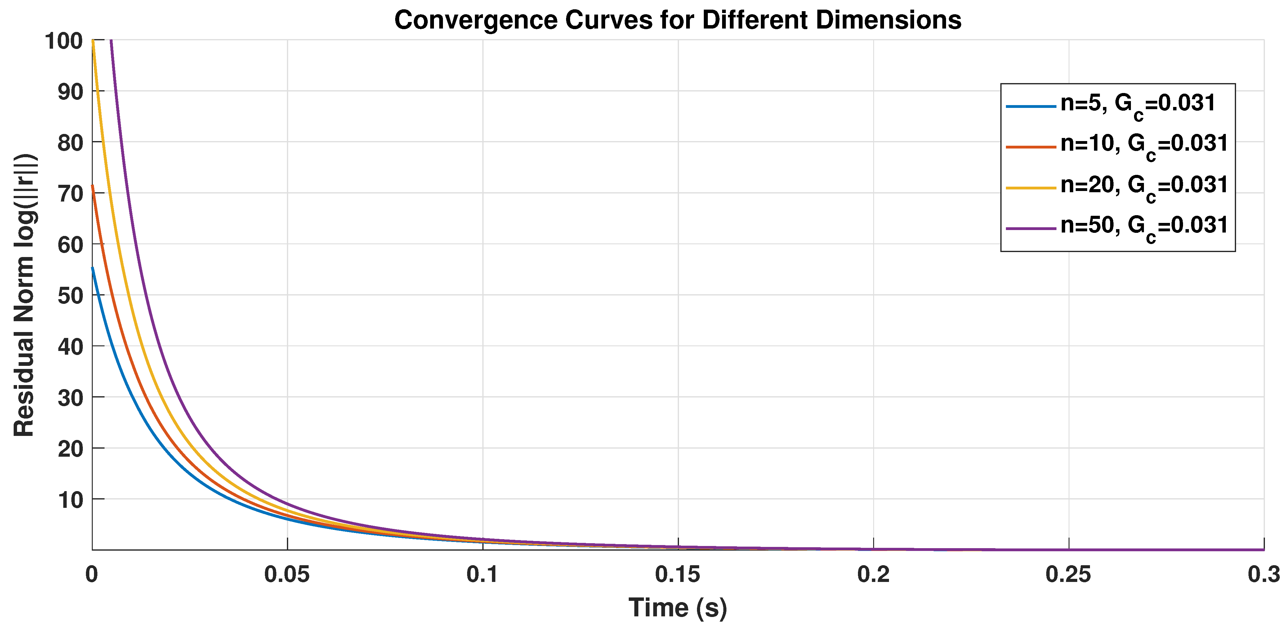
Case 1: The parameters are chosen as $T_c=1$, $\gamma =1$, ${\rho }_1=1$, ${\rho }_2=1$, ${\rho }_3=1$, ${\lambda }_1=0.5$, ${\lambda }_2=1.5$. Four different system dimensions $n=5,10,20,50$ were selected. Suppose that the initial point $x_0={[1,1,\cdots ,1]}^{\top }$. And the time interval was $t\in [0,3.0]$, and the step size was $0.0001$.

Table 2. Convergence performance of system (6) under different dimensions.

Dim (n)	${\mathit{\sigma }}_{\min }\left(\mathit{A}\right)$	$\parallel \mathit{B}\parallel$	${\mathit{G}}_{\mathit{c}}$	Final Residual	Convergence Time (s)
5	16.0000	0.3000	0.0314	$1.68\times {10}^{-7}$	0.2593
10	16.0000	0.3000	0.0314	$1.68\times {10}^{-7}$	0.2627
20	16.0000	0.3000	0.0314	$1.68\times {10}^{-7}$	0.2668
50	16.0000	0.3000	0.0314	$1.67\times {10}^{-7}$	0.2717

records the numerical results for dimensions $n=5,10,20,50$.

The data in Table 2 show that the algorithm maintains high numerical accuracy across different dimensions, and the convergence time increases only slightly as the dimension grows.

Figure 1 illustrates the convergence of the state estimation error $\parallel x\left(t\right)-x^{\ast }\parallel$ across different dimensions. And the convergence curves exhibit similar shapes for all tested dimensions, indicating consistent convergence behavior. This observation suggests that the convergence behavior is not only independent of the problem dimension, but also confirms the method’s practical applicability to large-scale GAVEs.

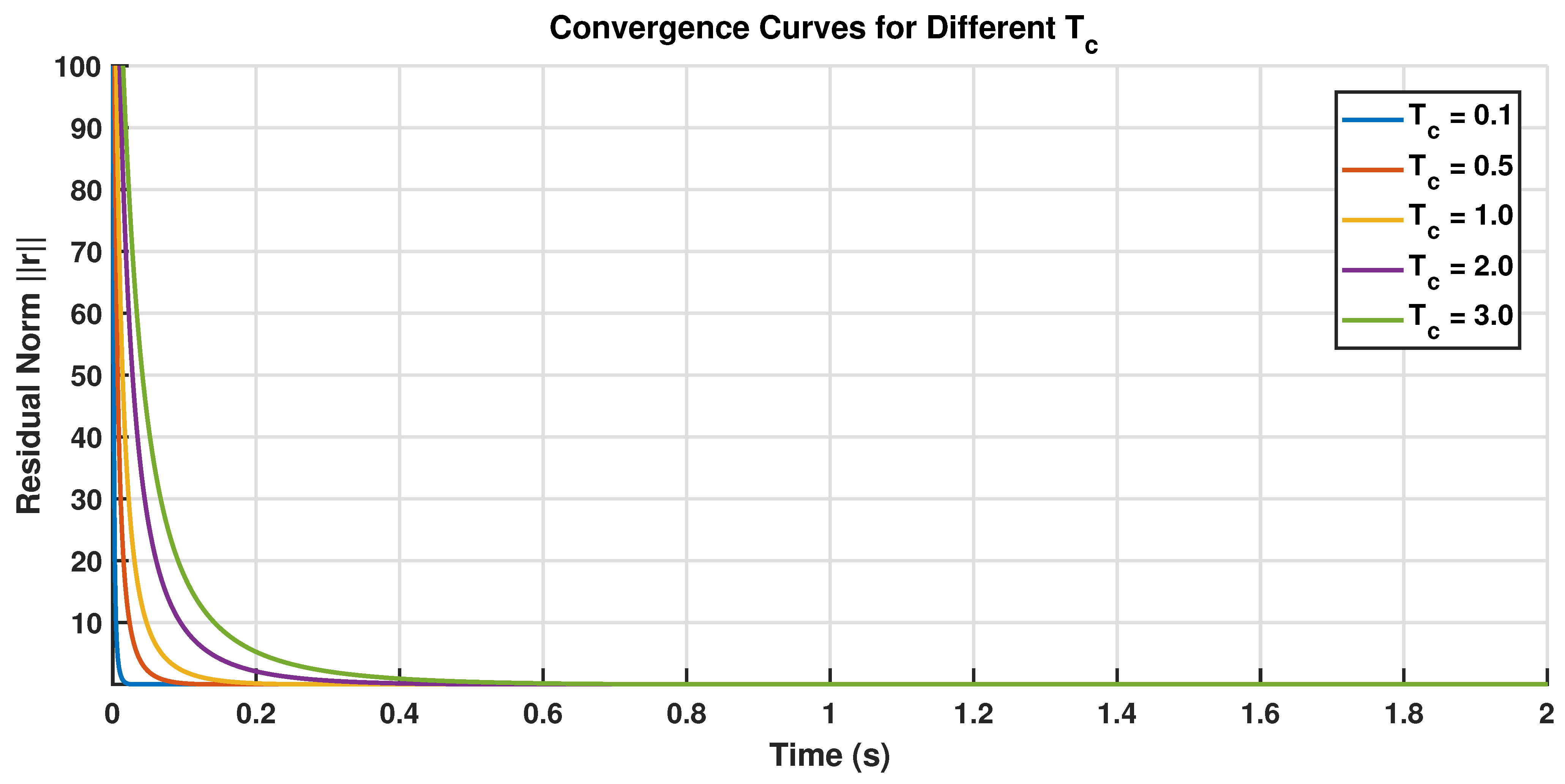
Case 2: Let $n=50$ and $T_c=0.1,0.5,1,2,3$ were selected.

Table 3. Convergence results for different $T_c$ values.

${\mathit{T}}_{\mathit{c}}$	Final Residual	Convergence Time (s)
0.1	$1.69\times {10}^{-5}$	0.0267
0.5	$6.70\times {10}^{-7}$	0.1356
1.0	$1.67\times {10}^{-7}$	0.2717
2.0	$4.18\times {10}^{-8}$	0.5439
3.0	$1.86\times {10}^{-8}$	0.8161

summarizes the performance for different $T_c$.

From Table 3, it can be observed that for all tested values of $T_c$, convergence was achieved within 3 s, with smaller $T_c$ leading to faster convergence times. Figure 2 shows that all curves eventually reach very low residuals, confirming that the approach can closely approximate the desired solution under the chosen $T_c$ and demonstrating the stability of the method. Two additional trends are observed. First, the convergence rate during the initial transient phase (e.g., for $t<0.5$ s) is dramatically faster for smaller $T_c$; specifically, for $T_c=0.1$, near-settlement is achieved within 0.1 s. Second, the final residual decreases monotonically as $T_c$ increases. This provides the user with a theoretical basis when designing the time upper bound.

Case 3: Let $T\left(n\right)$ denote the total computation time of the proposed algorithm for an n-dimensional system. We measured $T\left(n\right)$ for $n\in \{5,10,50,100,200,300\}$. All experiments were conducted under identical settings with a fixed time step $dt={10}^{-4}$ s and a simulation horizon $t_{\mathrm{end}}=3.0$ s. The results are summarized in

Table 4. Computational complexity evaluation: Running time vs. dimension.

Dimension n	Time $\mathit{T}\left(\mathit{n}\right)$ (s)	${\mathit{n}}^2$	$\mathit{T}\left(\mathit{n}\right)/{\mathit{n}}^2$	Final Residual
5	0.0267	25	$1.0674\times {10}^{-3}$	$1.68\times {10}^{-7}$
10	0.0248	100	$2.4780\times {10}^{-4}$	$1.68\times {10}^{-7}$
50	0.0872	2500	$3.4876\times {10}^{-5}$	$1.67\times {10}^{-7}$
100	0.6169	10,000	$6.1687\times {10}^{-5}$	$1.66\times {10}^{-7}$
200	1.3518	40,000	$3.3796\times {10}^{-5}$	$1.65\times {10}^{-7}$
300	2.5844	90,000	$2.8715\times {10}^{-5}$	$1.65\times {10}^{-7}$

.

For $n\ge 50$, the ratio $T\left(n\right)/n^2$ remains stable on the order of ${10}^{-5}$. The final residual remains consistently below $1.7\times {10}^{-7}$ for all tested dimensions.

The empirical results in Table 4 confirm that $T\left(n\right)/n^2$ remains stable for $n\ge 50$, which corroborates the theoretical $\mathcal{O}\left(n^2\right)$ complexity bound. The final residual remains below $1.7\times {10}^{-7}$ in all cases, indicating that the proposed algorithm converges reliably regardless of the problem size.

It follows from

Table 5. Computational cost analysis for different dimensions.

Dimension n	CPU Time (s)	Iterations	Final Error $\parallel \mathit{r}\parallel$	Status
5	0.0069	2594	$4.85\times {10}^{-4}$	Converged
10	0.0025	2628	$4.85\times {10}^{-4}$	Converged
50	0.0074	2718	$4.86\times {10}^{-4}$	Converged
100	0.0629	2755	$4.98\times {10}^{-4}$	Converged
200	0.1239	2791	$4.92\times {10}^{-4}$	Converged
300	0.2465	2807	$4.99\times {10}^{-4}$	Converged

that the approach performs consistently across all tested dimensions from $n=5$ to $n=300$, with final residuals stably maintained between $4.85\times {10}^{-4}$ and $4.99\times {10}^{-4}$, and the iteration numbers remain almost constant as the dimension increases, only gradually rising from 2594 to 2807, which verifies that the upper bound of the convergence time is independent of the system dimension.

The following Example 2 aims to validate the performance of the predefined-time system and analyze the convergence characteristics of the system within a given time frame.

Example 2.

Consider system (13) with the following five-dimensional experimental parameters: ${\lambda }_1=0.5$, ${\lambda }_2=2.0$, ${\rho }_1=2.0$, ${\rho }_2=1.0$, ${\rho }_3=0.5$, $\gamma =2.0$, $L=0.01$, and $T_c=2.0$. The system matrices are defined as

$$A=\left[\begin{array}{ccccc}10& -1& 0& 0& 0\\ -1& 10& -1& 0& 0\\ 0& -1& 10& -1& 0\\ 0& 0& -1& 10& -1\\ 0& 0& 0& -1& 10\end{array}\right]$$

and $B=0.3\times {\displaystyle \frac{B_0}{\parallel B_0{\parallel }_2}}$, where

$$B_0=\left[\begin{array}{ccccc}3& -0.5& 0& 0& 0\\ -0.5& 3& -0.5& 0& 0\\ 0& -0.5& 3& -0.5& 0\\ 0& 0& -0.5& 3& -0.5\\ 0& 0& 0& -0.5& 3\end{array}\right].$$

Let $c={[0.005,-0.005,0.005,-0.00,0.005]}^T$ and $\psi \left(x\right)=L\parallel x-x^{\ast }\parallel ·(x-x^{\ast })$. Through calculation, the system equilibrium point is obtained as

$$x^{\ast }={[0.00046889,-0.00040458,0.00042586,-0.00040458,0.00046889]}^T$$

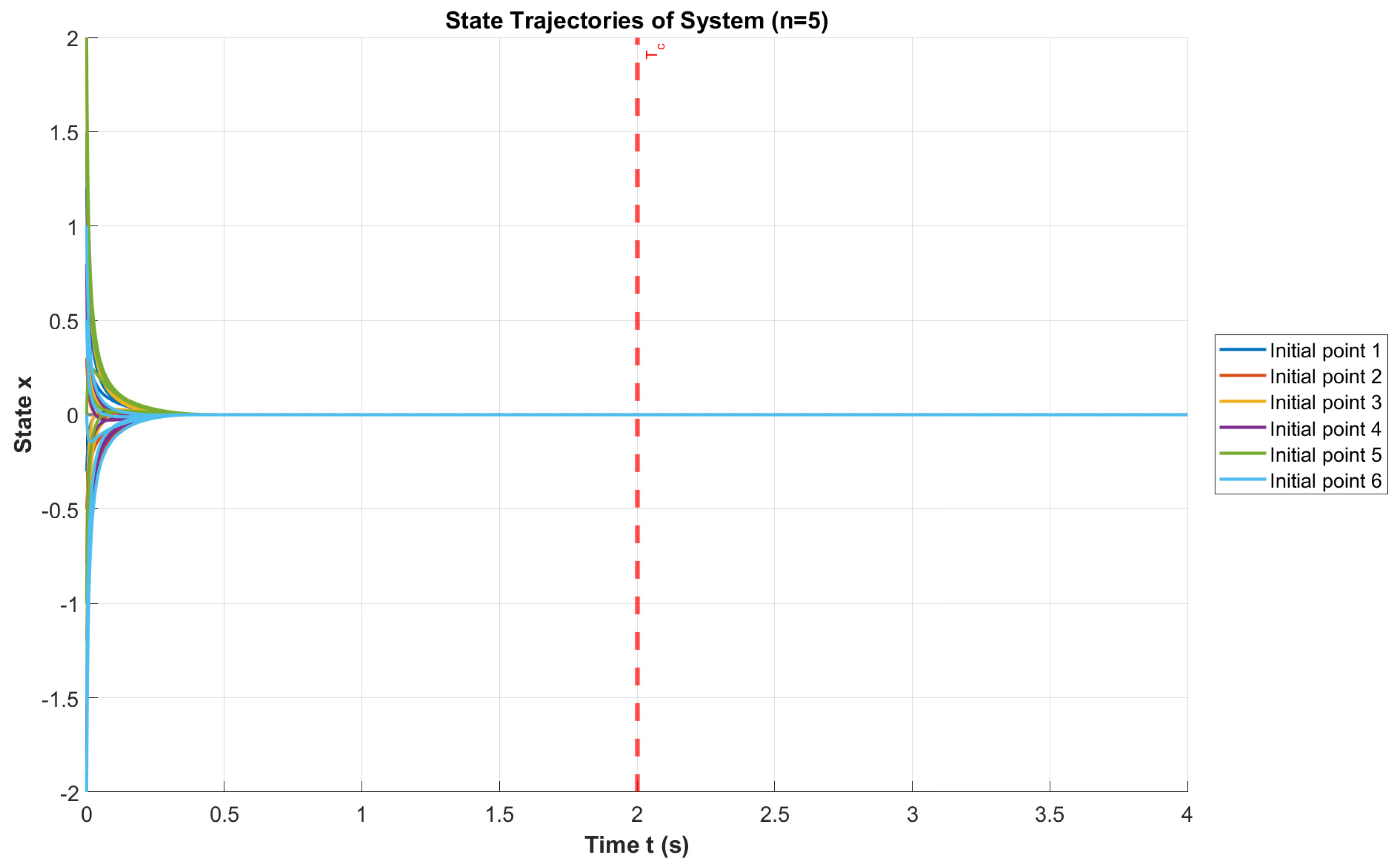
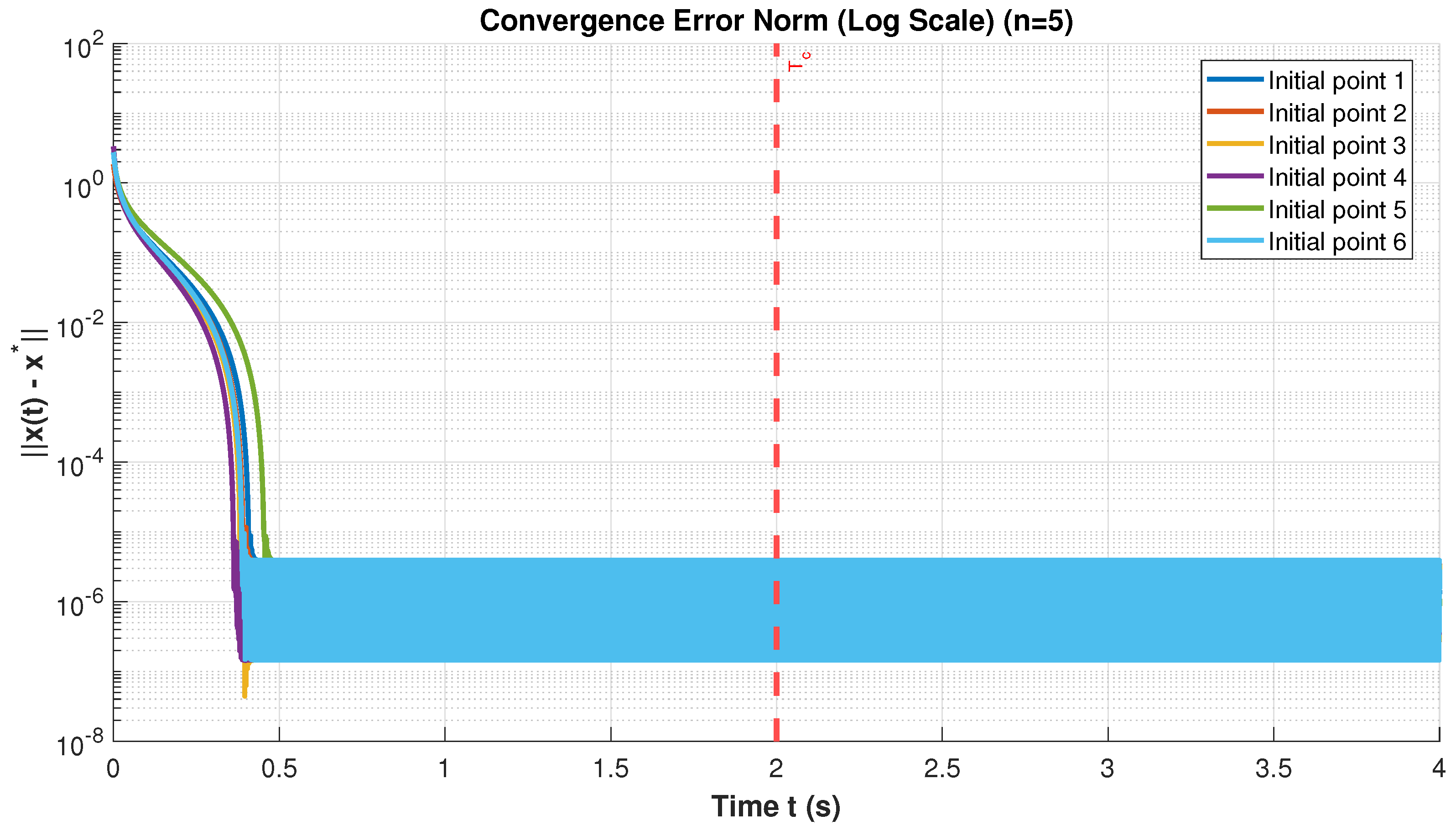
with $\parallel x^{\ast }\parallel =0.00097388$. Given that ${\sigma }_{\min }\left(A\right)=8.268$ and $\parallel B\parallel =0.300$, the condition ${\sigma }_{\min }\left(A\right)>\parallel B\parallel$ is satisfied. Six different initial vectors $x_0=\{x_0^1,x_0^2,x_0^3,x_0^4,x_0^5\}$ are used in this experiment, as specified in

Table 6. Six initial points for approach (6) under different initial points.

Initial Point No.	${\mathit{x}}_0^1$	${\mathit{x}}_0^2$	${\mathit{x}}_0^3$	${\mathit{x}}_0^4$	${\mathit{x}}_0^5$	$|{\mathit{x}}_0|$	$\parallel {\mathit{x}}_0-{\mathit{x}}^{\ast }\parallel$	Convergence Time
1	1.0000	0.5000	−0.8000	1.2000	−0.3000	1.8490	1.849703	0.3800
2	−1.0000	−0.5000	0.8000	−1.2000	0.3000	1.8490	1.848946	0.3640
3	2.0000	−1.5000	1.0000	−0.8000	1.8000	3.3360	3.335225	0.3540
4	−2.0000	1.5000	−1.0000	0.8000	−1.8000	3.3360	3.337106	0.3330
5	1.5000	0.0000	2.0000	−1.0000	0.5000	2.7390	2.737812	0.4250
6	0.0000	−2.0000	0.5000	1.0000	−1.5000	2.7390	2.738644	0.3600

.

It can be seen from Figure 3 that all trajectories converge to the equilibrium point within the predefined time $T_c=2.0$. The convergence process is smooth, without any overshoot or oscillation; furthermore, this consistent convergence behavior is observed across different initial conditions.

Figure 4 shows the convergence error norm in logarithmic scale. From Figure 4, we can get all six different initial conditions to converge and the disturbance $\psi \left(x\right)$ does not affect convergence. This implies that the system demonstrates robustness. In conclusion, we know that all test cases converge within $T_c=2.0$, the system exhibits strong robustness to initial conditions and external disturbances, and the convergence process is smooth and stable without oscillations.

Example 3.

Following the examples in [32], we compare the proposed method with several existing methods. Consider the GAVEs (1), with matrices A and B given by

$$A=\left[\begin{array}{cccccc}8& -1& 0& \cdots & 0& 0\\ -1& 8& -1& \cdots & 0& 0\\ ⋮& ⋮& ⋮& \ddots & ⋮& ⋮\\ 0& 0& 0& \cdots & 8& -1\\ 0& 0& 0& \cdots & -1& 8\end{array}\right],B=I-{\displaystyle \frac{v{v}^{\top }}{{\parallel v\parallel }^2}},v={[-\frac{1}{2},1,\cdots ,-\frac{1}{2},1]}^{\top }$$

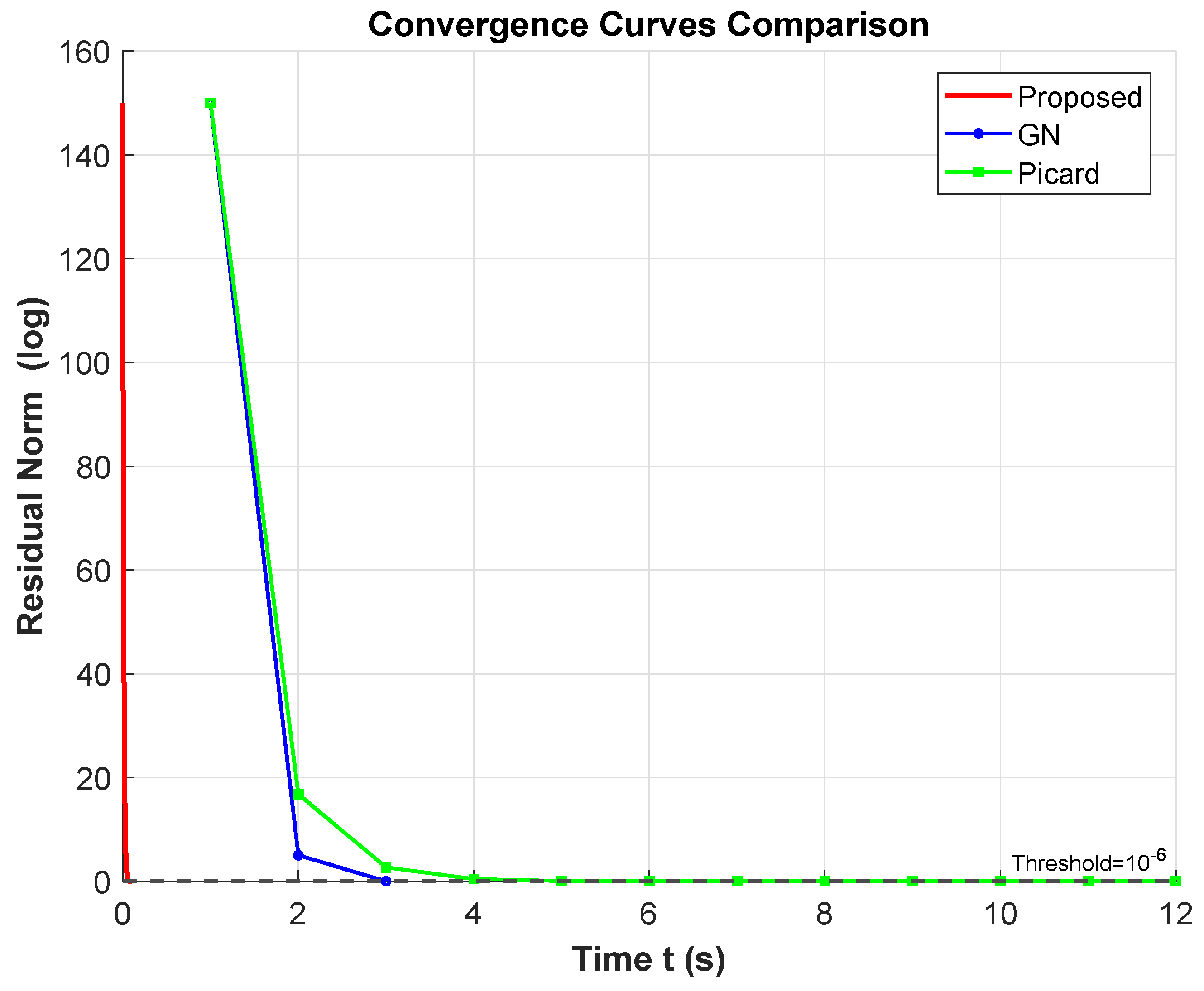
and $c=A{x}^{\ast }-B\left|x^{\ast }\right|$, where $x^{\ast }={[\frac{1}{2},1,\frac{1}{2},1,\cdots ,\frac{1}{2},1]}^{\top }\in {\mathbb{R}}^n$. The initial point is fixed as $x_0=\mathbf{0}\in {\mathbb{R}}^n$. The problem dimension is set to $n=1000$. The discretization step size is $\Delta t={10}^{-5}$ s, and the prescribed convergence time is $T_c=1.1G_c$, where $G_c$ is explicitly computed from Theorem 1. For the generalized Newton method [38] and the Picard iteration method [39], the maximum number of iterations is set to $K_{\max }={10}^4$. All methods adopt the same termination criterion: $\parallel A{x}_k-B|x_k|-c\parallel <{10}^{-6}$. For the proposed method, convergence is recorded at the first time such that the residual falls below ${10}^{-6}$. For system (6), the parameters are chosen as $\gamma =10$, $\xi =10$, ${\rho }_1=100$, ${\rho }_2={\displaystyle \frac{{\xi }^2{\pi }^2}{{\rho }_1{\left(\frac{{\sigma }_{\min }\left(A\right)}{{\parallel A\parallel }_2}\right)}^{1/\xi }{\varphi }^4}}$, ${\rho }_3=1$, ${\lambda }_1=0.9$, ${\lambda }_2=1.1$. Then show the convergence responses of the errors ${\log }_{10}{\parallel x\left(t\right)-x^{\ast }\parallel }_2^2$ compared with the Generalized Newton method, and the Picard iteration method for solving GAVEs.

The convergence curves in Figure 5 clearly demonstrate that the proposed method’s residual decreases monotonically. From Figure 5, we can observe that the proposed prescribed-time convergent dynamical system reduces the residual norm below the threshold of ${10}^{-6}$ within approximately $0.02$ s, demonstrating higher results compared to the other two methods.

5. Conclusions

This paper has introduced a novel neurodynamic approach for solving GAVEs. This approach ensures convergence to the unique solution within a user-defined time, independent of the initial state. Furthermore, we have rigorously established the robustness of the approach against perturbations. Future research will focus on the development of distributed neurodynamic approaches. Moreover, practical application scenarios of the proposed method are not further considered in this paper. In future work, we will investigate its applications in real-world engineering systems, such as unmanned aerial vehicles (UAVs) and robotic manipulators.

References

1. Wang, F.; Chen, J.; Huang, H.; Xu, S. A particle dynamical system algorithm to find the sparse linear complementary solutions. Appl. Soft Comput. 2024, 166, 112156. [Google Scholar] [CrossRef] [Scilit]
2. Ju, X.; Hu, D.; Li, C.; He, X.; Feng, G. A novel fixed-time converging neurodynamic approach to mixed variational inequalities and applications. IEEE Trans. Cybern. 2021, 52, 12942–12953. [Google Scholar] [CrossRef] [Scilit]
3. Ferris, M.C.; Pang, J.S. Engineering and economic applications of complementarity problems. Siam Rev. 1997, 39, 669–713. [Google Scholar] [CrossRef] [Scilit]
4. Mansoori, A.; Eshaghnezhad, M.; Effati, S. An efficient neural network model for solving the absolute value equations. IEEE Trans. Circuits Syst. II Express Briefs 2017, 65, 391–395. [Google Scholar] [CrossRef] [Scilit]
5. Rohn, J. Systems of linear interval equations. Linear Algebra Appl. 1989, 126, 39–78. [Google Scholar] [CrossRef] [Scilit]
6. Dang, T.M.; Nguyen, T.D.; Hoang, T.; Kim, H.; Teoh, A.B.J.; Choi, D. AVET: A novel transform function to improve cancellable biometrics security. IEEE Trans. Inf. Forensics Secur. 2022, 18, 758–772. [Google Scholar] [CrossRef] [Scilit]
7. Prokopyev, O. On equivalent reformulations for absolute value equations. Comput. Optim. Appl. 2009, 44, 363–372. [Google Scholar]
8. Wang, A.; Cao, Y.; Chen, J.X. Modified Newton-type iteration methods for generalized absolute value equations. J. Optim. Theory Appl. 2019, 181, 216–230. [Google Scholar]
9. Mangasarian, O.; Meyer, R. Absolute value equations. Linear Algebra Appl. 2006, 419, 359–367. [Google Scholar] [CrossRef] [Scilit]
10. Wu, S.L. The unique solution of a class of the new generalized absolute value equation. Appl. Math. Lett. 2021, 116, 107029. [Google Scholar] [CrossRef] [Scilit]
11. Hopfield, J.J.; Tank, D.W. “Neural” computation of decisions in optimization problems. Biol. Cybern. 1985, 52, 141–152. [Google Scholar] [CrossRef] [Scilit] [PubMed]
12. Lendaris, G.G.; Mathia, K.; Saeks, R. Linear Hopfield networks and constrained optimization. IEEE Trans. Syst. Man Cybern. Part B (Cybern.) 1999, 29, 114–118. [Google Scholar] [CrossRef] [Scilit]
13. Leung, M.F.; Wang, J. Cardinality-constrained portfolio selection based on collaborative neurodynamic optimization. Neural Netw. 2022, 145, 68–79. [Google Scholar] [CrossRef] [Scilit] [PubMed]
14. Wang, J.; Wu, G. A multilayer recurrent neural network for on-line synthesis of minimum-norm linear feedback control systems via pole assignment. Automatica 1996, 32, 435–442. [Google Scholar] [CrossRef] [Scilit]
15. Yang, S.; Liu, Q.; Wang, J. A collaborative neurodynamic approach to multiple-objective distributed optimization. IEEE Trans. Neural Netw. Learn. Syst. 2017, 29, 981–992. [Google Scholar] [CrossRef] [Scilit] [PubMed]
16. Bhat, S.P.; Bernstein, D.S. Finite-time stability of continuous autonomous systems. SIAM J. Control Optim. 2000, 38, 751–766. [Google Scholar] [CrossRef] [Scilit]
17. Polyakov, A. Nonlinear feedback design for fixed-time stabilization of linear control systems. IEEE Trans. Autom. Control 2011, 57, 2106–2110. [Google Scholar] [CrossRef] [Scilit]
18. Ju, X.; Li, C.; He, X.; Feng, G. A proximal dynamic approach to equilibrium problems with finite-time convergence. IEEE Trans. Autom. Control 2023, 69, 1773–1780. [Google Scholar] [CrossRef] [Scilit]
19. Sánchez-Torres, J.D.; Gómez-Gutiérrez, D.; López, E.; Loukianov, A.G. A class of predefined-time stable dynamical systems. IMA J. Math. Control Inf. 2018, 35, i1–i29. [Google Scholar]
20. Liu, H.; Yu, Z.; Jiang, H. Fixed-time consensus of nonlinear multi-agent systems via both event-triggered intermittent communication and sampled-data control. Commun. Nonlinear Sci. Numer. Simul. 2025, 140, 108391. [Google Scholar] [CrossRef] [Scilit]
21. Lu, Q.; Wu, X.; She, J.H.; Guo, F.H.; Yu, L. Disturbance rejection for systems with uncertainties based on fixed-time equivalent-input-disturbance approach. IEEE/CAA J. Autom. Sin. 2024, 11, 2384–2395. [Google Scholar] [CrossRef] [Scilit]
22. Yu, D.; Zhang, G.; Chen, C.; Han, D. The neural network models with delays for solving absolute value equations. Neurocomputing 2024, 589, 127707. [Google Scholar] [CrossRef] [Scilit]
23. Wei, J.; Chen, Z. Finite and fixed time synchronization of multi-link complex-valued complex networks with time delay via hybrid control. Commun. Nonlinear Sci. Numer. Simul. 2025, 144, 108678. [Google Scholar] [CrossRef] [Scilit]
24. Cai, Z.; Wang, Z.; Huang, L. Novel fixed/predefined-time stability of discontinuous time-varying system: State-feedback control of interconnected social networks. Commun. Nonlinear Sci. Numer. Simul. 2026, 152, 109447. [Google Scholar] [CrossRef] [Scilit]
25. Sun, Y.; Chen, Y.; Wang, B.; Ma, C. A novel adaptive predefined-time sliding mode control scheme for synchronizing fractional order chaotic systems. Chaos Solitons Fractals 2024, 189, 115610. [Google Scholar] [CrossRef] [Scilit]
26. Chen, C.; Yang, Y.; Yu, D.; Han, D. An inverse-free dynamical system for solving the absolute value equations. Appl. Numer. Math. 2021, 168, 170–181. [Google Scholar] [CrossRef] [Scilit]
27. Chen, J.; Sun, W.; Zheng, S. New predefined-time stability theorem and synchronization of fractional-order memristive delayed BAM neural networks. Commun. Nonlinear Sci. Numer. Simul. 2025, 148, 108850. [Google Scholar] [CrossRef] [Scilit]
28. Yu, D.; Zhang, G.; Ma, T. Neurodynamic approaches for solving absolute value equations and circuit implementation. Chaos Solitons Fractals 2025, 190, 115714. [Google Scholar] [CrossRef] [Scilit]
29. Zheng, J.; Ju, X.; Zhang, N.; Xu, D. A novel predefined-time neurodynamic approach for mixed variational inequality problems and applications. Neural Netw. 2024, 174, 106247. [Google Scholar] [CrossRef] [Scilit] [PubMed]
30. Ju, X.; Li, C.; Han, X.; He, X. Neurodynamic network for absolute value equations: A fixed-time convergence technique. IEEE Trans. Circuits Syst. II Express Briefs 2021, 69, 1807–1811. [Google Scholar] [CrossRef] [Scilit]
31. Lotfi, T.; Vieseh, H. A note on unique solvability of the absolute value equation. J. Linear Topol. Algebra 2013, 2, 77–81. [Google Scholar]
32. Li, X.; Chen, L.; Yu, D.; Chen, C.; Han, D. An inverse-free fixed-time stable dynamical system and its forward-Euler discretization for solving generalized absolute value equations. arXiv 2025, arXiv:2507.00531. [Google Scholar]
33. Khalil, H.K.; Grizzle, J.W. Nonlinear Systems; Prentice Hall: Upper Saddle River, NJ, USA, 2002; Volume 3. [Google Scholar]
34. Chen, C.; Li, L.; Peng, H.; Yang, Y.; Mi, L.; Zhao, H. A new fixed-time stability theorem and its application to the fixed-time synchronization of neural networks. Neural Netw. 2020, 123, 412–419. [Google Scholar] [CrossRef] [Scilit] [PubMed]
35. Feng, L.; Ju, X.; Lu, J.; Yang, X. Inverse-free neurodynamic optimization approach with time-varying coefficients for absolute value equations and its FPGA circuit implementation. Commun. Nonlinear Sci. Numer. Simul. 2026, 156, 109672. [Google Scholar] [CrossRef] [Scilit]
36. Ju, X.; Yang, X.; Feng, G.; Che, H. Neurodynamic optimization approaches with finite/fixed-time convergence for absolute value equations. Neural Netw. 2023, 165, 971–981. [Google Scholar] [CrossRef] [Scilit] [PubMed]
37. Lv, X.M.; Miao, S.X. A predefined-time neurodynamic model for solving absolute value equation. Neural Netw. 2026, 202, 109010. [Google Scholar] [CrossRef] [Scilit] [PubMed]
38. Hu, S.L.; Huang, Z.H.; Zhang, Q. A generalized Newton method for absolute value equations associated with second order cones. J. Comput. Appl. Math. 2011, 235, 1490–1501. [Google Scholar] [CrossRef] [Scilit]
39. Rohn, J.; Hooshyarbakhsh, V.; Farhadsefat, R. An iterative method for solving absolute value equations and sufficient conditions for unique solvability. Optim. Lett. 2014, 8, 35–44. [Google Scholar]
Figure 1. Comparison of Convergence Curves under Different Dimensions n.
Mathematics 14 02692 g001
Figure 2. Comparison of convergence curves under different T c .
Mathematics 14 02692 g002
Figure 3. Transient responses of system (13).
Mathematics 14 02692 g003
Figure 4. Error responses of system (13).
Mathematics 14 02692 g004
Figure 5. Comparison of three different methods.
Mathematics 14 02692 g005