Ensemble Extreme Learning Machines for Uncertainty Quantification in Ordinary Differential Equations

Abstract

This paper proposes an uncertainty-quantified surrogate framework for ordinary differential equations (ODEs) based on ensembles of extreme learning machines (ELMs). The method constructs $M=100$ independently randomized ELM surrogates for a given ODE trajectory, uses the ensemble mean as the predictor, and defines a pointwise ensemble spread as a preliminary uncertainty measure. To obtain statistically valid prediction intervals, a split-conformal calibration procedure is applied to the ensemble spread, yielding finite-sample marginal coverage under exchangeability while preserving computational efficiency, since each ELM is trained via a single ridge-regression solve. Theoretical results establish exact satisfaction of the prescribed initial condition, stability of the ensemble mean and variance with respect to perturbations in the training data, and almost-sure convergence of the empirical ensemble variance to the corresponding random-feature prediction variance. The hidden-layer sampling hypothesis is made explicit: the experiments use bounded hyperbolic-tangent features with independent uniform draws as the default and independent normal draws in sensitivity tests, both of which satisfy the finite-moment assumptions required by the convergence theorem. Comparisons with capacity-matched Bayesian random-feature neural surrogates and Monte Carlo dropout clarify differences in uncertainty representation. Numerical experiments on exponential, logistic, and damped oscillator dynamics demonstrate accurate reconstruction and calibrated uncertainty quantification in sparse and noisy regimes. Additional ablation studies quantify the effect of the denominator safeguard, calibration-sample size, ensemble size, training time, noise level, and hidden-parameter distribution.

1. Introduction

Uncertainty quantification (UQ) has become a central theme in scientific machine learning because accurate point predictions are insufficient when a learned surrogate is used for scientific inference, control, or forecasting. In differential-equation settings, the reliability of a learned trajectory is often as important as the trajectory itself, especially when data are sparse, noisy, or only partially informative. Recent work has therefore emphasized predictive uncertainty, calibration, and model misspecification in scientific machine learning, physics-informed learning, and universal differential equations; see, for instance, the broad UQ framework of Psaros et al. [1], the comparative study of Schmid et al. [2], and the recent analysis of total uncertainty in physics-informed reconstruction by De Florio et al. [3]. At the same time, Bayesian neural networks, Monte Carlo dropout, and deep ensembles remain widely used tools for uncertainty-aware neural modeling [4,5,6,7,8].

Extreme learning machines (ELMs), introduced by Huang, Zhu, and Siew [9], provide a computationally economical random-feature paradigm. In a single-hidden-layer feedforward network, the hidden parameters are sampled randomly and then frozen, while the output layer is learned analytically. This yields a training procedure that is much cheaper than iterative gradient-based optimization. The basic theory and regression properties of ELMs are well established [9,10], and randomized-feature versions of ELM ideas have recently been used successfully for numerical differential equations and scientific computing, including collocation for PDEs [11,12] and Bayesian physics-informed ELM variants for noisy PDE problems [13]. In parallel, Guignard, Amato, and Kanevski [14] developed a careful study of variability and interval estimation for ELM regression in generic supervised settings.

The present work differs from the general ELM regression uncertainty analysis of Guignard et al. [14] in four concrete ways. First, the target object here is an ODE trajectory represented through an initial-condition-preserving trial form, rather than a generic regression map. Second, the hidden-layer randomization is used as a random-feature ensemble for trajectory reconstruction, while the output weights are still obtained by closed-form ridge solves. Third, raw ensemble spread is treated only as a local nonconformity scale; calibrated coverage is supplied by a split-conformal step. Fourth, the theoretical statements are formulated around ODE trajectory bands, exact initial-condition enforcement, response stability of the ELM smoother, random-feature variance convergence, and pointwise marginal conformal coverage. These ingredients make the method closer to a calibrated numerical surrogate than to a general-purpose ELM regression interval.

The proposed ensemble also differs from deep ensembles [6]. A deep ensemble trains several independently initialized deep networks by iterative optimization and typically interprets the diversity of the trained networks as epistemic uncertainty. The present construction uses a single-hidden-layer random-feature architecture; only the output layer is trained, each member is obtained from one ridge solve, and the ensemble spread is passed through a distribution-free calibration layer. Thus the uncertainty band is tied to randomized-feature variability plus conformal calibration, rather than to optimizer-dependent diversity among separately trained deep models. This distinction is important in sparse ODE reconstruction, where a lightweight ensemble can be generated with little computational cost and then calibrated on held-out trajectory values.

The problem considered in this paper is novel in a precise sense. The existing ELM-UQ literature studies either generic supervised regression variability [14] or Bayesian output-layer formulations for PDEs [13], while ODE and scientific-machine-learning UQ studies are dominated by Bayesian, variational, dropout, and physics-informed neural approaches [1,2,3,15]. The combination developed here—initial-condition-preserving ELM trajectory reconstruction, independently randomized hidden layers, spread-normalized conformal scores, and a finite-sample marginal coverage theorem—appears to have been formalized only partially in the existing literature. It is this combination of computational speed, ODE-specific reconstruction, and calibrated uncertainty that motivates the present work.

The main methodological idea is intentionally simple. We represent the unknown ODE trajectory by a trial function that satisfies the initial condition exactly. We then fit $M=100$ independently randomized ELMs to training data generated by an ODE solution or a trusted numerical solver. The ensemble mean becomes the point predictor. The empirical spread of the ensemble quantifies how much the random hidden-layer realization changes the reconstructed trajectory. Because raw ensemble spread alone does not guarantee calibrated uncertainty, we normalize calibration residuals by the ensemble spread and use split conformal prediction [16,17] to obtain finite-sample valid predictive bands under exchangeability. This construction is particularly attractive in ODE applications because the ELM members are fast to train and trivially parallelizable and the conformal adjustment is model-agnostic.

The contributions of the paper are fourfold. The first contribution is methodological: we formulate an ensemble ELM architecture for ODE trajectory reconstruction in which every member satisfies the initial condition exactly and is trained by a closed-form ridge solve. The second contribution is theoretical: we prove a linear smoother representation, derive stability bounds for both the ensemble mean and ensemble spread, establish almost-sure convergence of the empirical spread to the random-feature variance, and obtain a finite-sample marginal coverage theorem for a conformalized ensemble interval. The third contribution is comparative: we place the proposed interval next to Bayesian and dropout-based uncertainty mechanisms, proving that exact Bayesian predictive coverage requires a correctly specified probabilistic model, while Monte Carlo dropout intervals quantify mask randomness and require additional calibration or noise modeling for coverage in biased or noisy settings. The fourth contribution is applied: we carry out a reproducible ODE benchmark study based on sparse and noisy observations of exponential, logistic, and damped-oscillator dynamics, together with calibration, sharpness, ablation, noise-sensitivity, and timing diagnostics.

The paper is organized as follows. Section 2 introduces the ODE reconstruction setting, the data model, the hidden-layer sampling distribution, and the ensemble ELM architecture. Section 3 defines the conformalized spread-based interval and records the training and calibration procedure. Section 4 contains the main theoretical results and their proofs, including the comparison principles for Bayesian and dropout baselines. Section 5 reports the numerical experiments and discusses the observed calibration-sharpness trade-off, ablation results, noise sensitivity, and computational scaling. Section 6 concludes the paper.

2. Preliminaries

Consider a scalar initial-value problem

$$\left\{\begin{array}{c}{u}^{\prime }\left(t\right)=f(t,u\left(t\right)),t\in [0,T],\hfill \\ u\left(0\right)=u_0,\hfill \end{array}\right.$$

(1)

where $f:[0,T]\times \mathbb{R}\to \mathbb{R}$ is continuous and the solution u is assumed unique on $[0,T]$. The scalar formulation is adopted for clarity of proofs; vector-valued systems are handled componentwise or by block-design matrices, and the same arguments remain valid with only notational modifications.

We assume that one has access to reference trajectory values at design times $0=t_1<t_2<\dots <t_n\le T$. These values may come from a trusted numerical solver, a high-fidelity simulator, or sufficiently accurate measurements. Denote the response vector by

$$\mathit{y}={(y_1,\dots ,y_n)}^{\top },y_i\approx u\left(t_i\right),$$

with the punctuation included here and below to make the displayed formulae part of the surrounding sentences. When noisy observations are used, one may write $y_i=u\left(t_i\right)+{\epsilon }_i$ with mean-zero noise ${\epsilon }_i$. Since the focus of the present paper is confidence bands for the reconstructed trajectory itself, the clean-state setting is emphasized in the theory; noisy-response coverage can be handled by adding an independent noise term or by calibrating against observed responses instead of latent states.

The defining feature of the surrogate is that the initial condition is enforced exactly through the trial form

$$\widehat{u}\left(t\right)=u_0+tg\left(t\right),$$

(2)

where g is represented by a single-hidden-layer randomized neural network. Thus, regardless of how g is fitted, one always has $\widehat{u}\left(0\right)=u_0$.

For a hidden width $m\in \mathbb{N}$ and an activation function $\sigma :\mathbb{R}\to \mathbb{R}$, define a random feature map

$${\varphi }_{\omega }\left(t\right)={\left(\sigma (a_{1}t+b_1),\dots ,\sigma (a_{m}t+b_m)\right)}^{\top },$$

where $\omega =((a_1,b_1),\dots ,(a_m,b_m))$ is sampled from a distribution $\Pi$ on ${\mathbb{R}}^{2m}$. The kth ELM member uses an independent draw ${\omega }_k$ and models

$${\widehat{u}}_k\left(t\right)=u_0+h_k{\left(t\right)}^{\top }{\widehat{\beta }}_k,h_k\left(t\right)=t{\varphi }_{{\omega }_k}\left(t\right)\in {\mathbb{R}}^m.$$

(3)

In all numerical experiments the physical time is first scaled to $[0,1]$ before random features are formed. The default hidden-layer distribution is the product law

$$a_j\stackrel{\mathrm{i}.\mathrm{i}.\mathrm{d}.}{\sim }Unif[-12,12],b_j\stackrel{\mathrm{i}.\mathrm{i}.\mathrm{d}.}{\sim }Unif[-3,3],j=1,\dots ,m,$$

with independent draws across hidden units and across ensemble members. A normal-sampling sensitivity test uses

$$a_j\stackrel{\mathrm{i}.\mathrm{i}.\mathrm{d}.}{\sim }N(0,3^2),b_j\stackrel{\mathrm{i}.\mathrm{i}.\mathrm{d}.}{\sim }N(0,3^2).$$

The selection criteria for $\Pi$ are as follows: independent sampling across ensemble members, non-degenerate hidden features on the scaled time interval, and finite fourth moments of the resulting pointwise predictions after ridge fitting. For the bounded activation $\sigma =tanh$ used here, both the uniform and normal choices satisfy these criteria automatically; the verification is given in Lemma 2.

With the design matrix

$$H_k=\left(\begin{array}{c}{h}_k{\left(t_1\right)}^{\top }\\ ⋮\\ h_k{\left(t_n\right)}^{\top }\end{array}\right)\in {\mathbb{R}}^{n\times m},$$

and centered response vector

$${\mathit{y}}^{\circ }=\mathit{y}-u_0{\mathbf{1}}_n,$$

we compute the ridge-regression output weights by

$${\widehat{\beta }}_k={(H_k^{\top }{H}_k+\lambda I_m)}^{-1}{H}_k^{\top }{\mathit{y}}^{\circ },\lambda >0.$$

(4)

The ridge parameter $\lambda$ is included for stability and to avoid singularity when $m>n$ or the sampled features are nearly collinear.

The ensemble contains $M=100$ independent members throughout the main applied study, although the theory is stated for a generic positive integer M. The ensemble mean and empirical spread are defined pointwise by

$${\overline{u}}_M\left(t\right)={\displaystyle \frac{1}{M}}{\displaystyle \sum _{k=1}^M}{\widehat{u}}_k\left(t\right),s_M^2\left(t\right)={\displaystyle \frac{1}{M-1}}{\displaystyle \sum _{k=1}^M}{\left({\widehat{u}}_k\left(t\right)-{\overline{u}}_M\left(t\right)\right)}^2.$$

(5)

The quantity $s_M\left(t\right)$ is the primitive uncertainty score produced by the randomized ensemble. It measures the sensitivity of the reconstruction to the hidden-layer randomization and, as shown below, converges to the random-feature prediction variance when M grows.

3. Conformalized Ensemble-ELM Uncertainty Bands

A raw interval of the form

$${\overline{u}}_M\left(t\right)\pm z_{1-\alpha /2}{s}_M\left(t\right),$$

is easy to compute but has no universal coverage guarantee. In particular, the empirical spread only reflects the variability induced by the random feature draw; it may fail to account for model bias, heteroscedasticity, or local approximation error. To obtain a coverage statement that does not rely on a correct probabilistic model, we calibrate the spread by split conformal prediction.

We split the available design points into a training set ${\mathcal{I}}_{\mathrm{tr}}$ and a calibration set ${\mathcal{I}}_{\mathrm{cal}}$, with cardinalities $n_{\mathrm{tr}}$ and $n_{\mathrm{cal}}$, respectively. All M ELM members are trained using only the training set. Then, for each calibration point $i\in {\mathcal{I}}_{\mathrm{cal}}$, we compute the nonconformity score

$$R_i={\displaystyle \frac{\left|y_i-{\overline{u}}_M\left(t_i\right)\right|}{s_M\left(t_i\right)+\gamma }},$$

(6)

where $\gamma >0$ is a small denominator safeguard. Let $R_{\left(1\right)}\le \dots \le R_{\left(n_{\mathrm{cal}}\right)}$ be the order statistics of the calibration scores, and define

$$q_{1-\alpha }=R_{\left(⌈(n_{\mathrm{cal}}+1)(1-\alpha )⌉\right)}.$$

(7)

The proposed pointwise uncertainty band is then

$${\mathcal{C}}_{\alpha }\left(t\right)=\left[{\overline{u}}_M\left(t\right)-q_{1-\alpha }\left(s_M\left(t\right)+\gamma \right),{\overline{u}}_M\left(t\right)+q_{1-\alpha }\left(s_M\left(t\right)+\gamma \right)\right].$$

(8)

The width adapts locally through $s_M\left(t\right)$, while the conformal factor $q_{1-\alpha }$ corrects global under- or over-dispersion of the raw ensemble uncertainty.

The value of $\gamma$ is a numerical regularization parameter for small-spread regions. It prevents a calibration residual from being divided by an empirical ensemble standard deviation that is close to zero. The experiments use $\gamma =5\times {10}^{-3}$ in the response units of each benchmark, and Section 5.4 reports a sensitivity analysis over $\gamma \in \{0,{10}^{-4},{10}^{-3},5\times {10}^{-3},{10}^{-2}\}$ and $n_{\mathrm{cal}}\in \{10,15,20,30\}$.

The training and calibration steps are therefore as follows. First, sample $M=100$ independent hidden-layer parameter sets and fit the corresponding ELM output weights by (4). Second, evaluate the ensemble mean and spread at the calibration inputs. Third, form the normalized residuals (6) and compute the empirical conformal quantile (7). Finally, report the interval (8) on any desired time grid. The procedure is non-iterative at the ELM level, parallel across ensemble members, and agnostic to the particular ODE generating the trajectory data.

The conformal theorem in Section 3 is a pointwise marginal statement under exchangeability of the calibration pair and the future pair after the training split has been fixed. For deterministic high-fidelity ODE values sampled at randomized design points, this can be read as coverage over the randomized design-and-split mechanism. For observational time series with serially correlated measurement errors, the exchangeability condition becomes a modeling assumption that should be replaced by a block, trajectory-level, or other dependence-aware conformal construction. The present experiments use independent observation noise and random train/calibration splits, so the numerical study probes the stated pointwise calibration mechanism rather than simultaneous-in-time coverage of an entire dependent path.

4. Main Results

We now present the main results. The first lemma records the exact initial-condition property and the linear smoother form of each ensemble member. The next theorem gives stability estimates for the ensemble mean and spread. We then establish almost sure convergence of the empirical spread and the finite-sample coverage theorem for the conformalized interval. The section ends with two comparison propositions clarifying how the proposed uncertainty mechanism differs from ideal Bayesian prediction and Monte Carlo dropout.

Lemma 1. 

For each ensemble member $k\in \{1,\dots ,M\}$, the predictor (3)–(4) satisfies ${\widehat{u}}_k\left(0\right)=u_0$. Moreover,

$${\widehat{u}}_k\left(t\right)=u_0+{\mathsf{\ell }}_k{\left(t\right)}^{\top }{\mathit{y}}^{\circ },{\mathsf{\ell }}_k\left(t\right)=H_k{(H_k^{\top }{H}_k+\lambda I_m)}^{-1}{h}_k\left(t\right)\in {\mathbb{R}}^n.$$

(9)

Hence each ELM member is a linear smoother in the responses.

Proof. 

Since $h_k\left(t\right)=t{\varphi }_{{\omega }_k}\left(t\right)$, we have $h_k\left(0\right)=\mathbf{0}$, and therefore from (3)

$${\widehat{u}}_k\left(0\right)=u_0+h_k{\left(0\right)}^{\top }{\widehat{\beta }}_k=u_0.$$

This proves the initial-condition statement.

For the linear smoother representation, substitute (4) into (3):

$${\widehat{u}}_k\left(t\right)=u_0+h_k{\left(t\right)}^{\top }{(H_k^{\top }{H}_k+\lambda I_m)}^{-1}{H}_k^{\top }{\mathit{y}}^{\circ }.$$

The right-hand side is a scalar. Using the identity $a^{\top }Bc={\left(B^{\top }a\right)}^{\top }c$ and the symmetry of ${(H_k^{\top }{H}_k+\lambda I_m)}^{-1}$, we obtain

$${\widehat{u}}_k\left(t\right)=u_0+{\left(H_k{(H_k^{\top }{H}_k+\lambda I_m)}^{-1}{h}_k\left(t\right)\right)}^{\top }{\mathit{y}}^{\circ }=u_0+{\mathsf{\ell }}_k{\left(t\right)}^{\top }{\mathit{y}}^{\circ },$$

which is exactly (9). The dependence on the responses is therefore linear. This completes the proof. □

Theorem 1. 

Fix $t\in [0,T]$. For the kth ensemble member define

$$C_k\left(t\right)={\displaystyle \frac{\parallel h_k{\left(t\right)\parallel }_2{\parallel H_k\parallel }_2}{\lambda }}.$$

Then for any two response vectors $\mathit{y},\tilde{\mathit{y}}\in {\mathbb{R}}^n$ with centered versions ${\mathit{y}}^{\circ },{\tilde{\mathit{y}}}^{\circ }$, one has

$$\left|{\widehat{u}}_k(t;\mathit{y})-{\widehat{u}}_k(t;\tilde{\mathit{y}})\right|\le C_k\left(t\right){\parallel {\mathit{y}}^{\circ }-{\tilde{\mathit{y}}}^{\circ }\parallel }_2.$$

(10)

Consequently,

$$\left|{\overline{u}}_M(t;\mathit{y})-{\overline{u}}_M(t;\tilde{\mathit{y}})\right|\le \left({\displaystyle \frac{1}{M}}{\displaystyle \sum _{k=1}^M}{C}_k\left(t\right)\right){\parallel {\mathit{y}}^{\circ }-{\tilde{\mathit{y}}}^{\circ }\parallel }_2,$$

(11)

and

$$\left|s_M(t;\mathit{y})-s_M(t;\tilde{\mathit{y}})\right|\le {\left({\displaystyle \frac{{\sum }_{k=1}^M{C}_k{\left(t\right)}^2}{M-1}}\right)}^{1/2}{\parallel {\mathit{y}}^{\circ }-{\tilde{\mathit{y}}}^{\circ }\parallel }_2.$$

(12)

Proof. 

Let

$$A_k={(H_k^{\top }{H}_k+\lambda I_m)}^{-1}{H}_k^{\top }.$$

Using (3), we write

$${\widehat{u}}_k(t;\mathit{y})-{\widehat{u}}_k(t;\tilde{\mathit{y}})=h_k{\left(t\right)}^{\top }{A}_k({\mathit{y}}^{\circ }-{\tilde{\mathit{y}}}^{\circ }).$$

Therefore,

$$\left|{\widehat{u}}_k(t;\mathit{y})-{\widehat{u}}_k(t;\tilde{\mathit{y}})\right|\le \parallel h_k{\left(t\right)\parallel }_2\parallel A_k{\parallel }_2{\parallel {\mathit{y}}^{\circ }-{\tilde{\mathit{y}}}^{\circ }\parallel }_2.$$

Now

$${\parallel A_k\parallel }_2=\parallel {(H_k^{\top }{H}_k+\lambda I_m)}^{-1}{H}_k^{\top }{\parallel }_2\le \parallel {(H_k^{\top }{H}_k+\lambda I_m)}^{-1}{\parallel }_2{\parallel H_k\parallel }_2.$$

Since the smallest eigenvalue of $H_k^{\top }{H}_k+\lambda I_m$ is at least $\lambda$, we have

$${\parallel {(H_k^{\top }{H}_k+\lambda I_m)}^{-1}\parallel }_2\le {\displaystyle \frac{1}{\lambda }}.$$

Combining the last three displays proves (10).

To obtain (11), average (10) over $k=1,\dots ,M$ and use the following triangle inequality:

$$\left|{\overline{u}}_M(t;\mathit{y})-{\overline{u}}_M(t;\tilde{\mathit{y}})\right|\le {\displaystyle \frac{1}{M}}{\displaystyle \sum _{k=1}^M}\left|{\widehat{u}}_k(t;\mathit{y})-{\widehat{u}}_k(t;\tilde{\mathit{y}})\right|\le \left({\displaystyle \frac{1}{M}}{\displaystyle \sum _{k=1}^M}{C}_k\left(t\right)\right){\parallel {\mathit{y}}^{\circ }-{\tilde{\mathit{y}}}^{\circ }\parallel }_2.$$

For the spread, let

$$\mathit{v}={({\widehat{u}}_1(t;\mathit{y}),\dots ,{\widehat{u}}_M(t;\mathit{y}))}^{\top },\tilde{\mathit{v}}={({\widehat{u}}_1(t;\tilde{\mathit{y}}),\dots ,{\widehat{u}}_M(t;\tilde{\mathit{y}}))}^{\top }.$$

Let $P=I_M-{\displaystyle \frac{1}{M}}{\mathbf{1}}_M{\mathbf{1}}_M^{\top }$ be the centering matrix. Then

$$s_M(t;\mathit{y})={\displaystyle \frac{{\parallel P\mathit{v}\parallel }_2}{\sqrt{M-1}}},s_M(t;\tilde{\mathit{y}})={\displaystyle \frac{\parallel P\tilde{\mathit{v}}{\parallel }_2}{\sqrt{M-1}}}.$$

Hence,

$$\left|s_M(t;\mathit{y})-s_M(t;\tilde{\mathit{y}})\right|\le {\displaystyle \frac{1}{\sqrt{M-1}}}\parallel P(\mathit{v}-\tilde{\mathit{v}}){\parallel }_2\le {\displaystyle \frac{1}{\sqrt{M-1}}}{\parallel \mathit{v}-\tilde{\mathit{v}}\parallel }_2,$$

because ${\parallel P\parallel }_2\le 1$. Using (10) componentwise gives

$$\parallel \mathit{v}-\tilde{\mathit{v}}{\parallel }_2^2={\displaystyle \sum _{k=1}^M}{\left|{\widehat{u}}_k(t;\mathit{y})-{\widehat{u}}_k(t;\tilde{\mathit{y}})\right|}^2\le \left({\displaystyle \sum _{k=1}^M}{C}_k{\left(t\right)}^2\right){\parallel {\mathit{y}}^{\circ }-{\tilde{\mathit{y}}}^{\circ }\parallel }_2^2.$$

Taking square roots yields (12). The proof is complete.

□

Lemma 2 

(Finite-moment verification for the hidden-layer sampling). Fix a compact interval $[0,T]$, a finite training vector $\mathit{y}$, a ridge parameter $\lambda >0$, and the bounded activation $\sigma =tanh$. Then, for every fixed $t\in [0,T]$, the random prediction ${\widehat{u}}_1\left(t\right)$ generated by (3)–(4) has finite fourth moment under both the uniform and normal hidden-parameter laws specified in Section 2.

Proof. 

For $\sigma =tanh$, each hidden feature satisfies $\left|\sigma \right(a_{j}t+b_j\left)\right|\le 1$. Therefore $\parallel h_1{\left(t\right)\parallel }_2\le T\sqrt{m}$ and $\parallel H_1{\parallel }_2\le T\sqrt{nm}$ for every realization of the hidden parameters. From (4),

$${\parallel {\widehat{\beta }}_1\parallel }_2\le \parallel {(H_1^{\top }{H}_1+\lambda I_m)}^{-1}{\parallel }_2\parallel H_1{\parallel }_2\parallel {\mathit{y}}^{\circ }{\parallel }_2\le {\displaystyle \frac{T\sqrt{nm}}{\lambda }}{\parallel {\mathit{y}}^{\circ }\parallel }_2.$$

Consequently,

$$\left|{\widehat{u}}_1\left(t\right)\right|\le \left|u_0\right|+\parallel h_1{\left(t\right)\parallel }_2\parallel {\widehat{\beta }}_1{\parallel }_2\le |u_0|+{\displaystyle \frac{T^{2}m\sqrt{n}}{\lambda }}{\parallel {\mathit{y}}^{\circ }\parallel }_2.$$

The final bound is deterministic and finite. Hence $\mathbb{E}\left(\right|{\widehat{u}}_1\left(t\right){|}^4\mid {\mathcal{D}}_{\mathrm{tr}})<\infty$. The argument uses only the boundedness of the activation and the ridge parameter, so it applies equally to the stated uniform and normal laws for the hidden weights and biases. □

Theorem 2. 

Fix $t\in [0,T]$ and condition on the training data. Suppose that the ensemble members ${\widehat{u}}_1\left(t\right),{\widehat{u}}_2\left(t\right),\dots$ are independent and identically distributed through the random hidden-layer draws, and that

$$\mathbb{E}\left[|{\widehat{u}}_1{\left(t\right)|}^4\mid {\mathcal{D}}_{\mathrm{tr}}\right]<\infty .$$

Lemma 2 verifies this condition for the uniform and normal hidden-layer sampling laws used in the numerical experiments. Define

$$\mu \left(t\right)=\mathbb{E}\left[{\widehat{u}}_1\left(t\right)\mid {\mathcal{D}}_{\mathrm{tr}}\right],v\left(t\right)=Var\left({\widehat{u}}_1\left(t\right)\mid {\mathcal{D}}_{\mathrm{tr}}\right).$$

Then, as $M\to \infty$,

$${\overline{u}}_M\left(t\right)\to \mu \left(t\right)\mathit{almost}\mathit{surely},$$

(13)

and

$$s_M^2\left(t\right)\to v\left(t\right)\mathrm{almost}\mathrm{surely}.$$

(14)

In particular, the empirical ensemble spread converges almost surely to the random-feature predictive standard deviation.

Proof. 

Conditional on the training data, the random variables ${\widehat{u}}_1\left(t\right),{\widehat{u}}_2\left(t\right),\dots$ are i.i.d. with finite first moment, because the assumed finite fourth moment implies finite first and second moments. By the strong law of large numbers,

$${\displaystyle \frac{1}{M}}{\displaystyle \sum _{k=1}^M}{\widehat{u}}_k\left(t\right)\to \mathbb{E}\left[{\widehat{u}}_1\left(t\right)\mid {\mathcal{D}}_{\mathrm{tr}}\right]=\mu \left(t\right)\mathrm{almost}\mathrm{surely}.$$

This is exactly (13).

Again, by the strong law of large numbers applied to the square, we have

$${\displaystyle \frac{1}{M}}{\displaystyle \sum _{k=1}^M}{\widehat{u}}_k{\left(t\right)}^2\to \mathbb{E}\left[{\widehat{u}}_1{\left(t\right)}^2\mid {\mathcal{D}}_{\mathrm{tr}}\right]\mathrm{almost}\mathrm{surely}.$$

Recall the identity

$$s_M^2\left(t\right)={\displaystyle \frac{M}{M-1}}\left({\displaystyle \frac{1}{M}}{\displaystyle \sum _{k=1}^M}{\widehat{u}}_k{\left(t\right)}^2-{\left({\displaystyle \frac{1}{M}}{\displaystyle \sum _{k=1}^M}{\widehat{u}}_k\left(t\right)\right)}^2\right).$$

Since $M/(M-1)\to 1$, the first average converges almost surely to $\mathbb{E}[{\widehat{u}}_1{\left(t\right)}^2\mid {\mathcal{D}}_{\mathrm{tr}}]$, and the second term converges almost surely to $\mu {\left(t\right)}^2$. Therefore,

$$s_M^2\left(t\right)\to \mathbb{E}\left[{\widehat{u}}_1{\left(t\right)}^2\mid {\mathcal{D}}_{\mathrm{tr}}\right]-\mu {\left(t\right)}^2=Var\left({\widehat{u}}_1\left(t\right)\mid {\mathcal{D}}_{\mathrm{tr}}\right)=v\left(t\right)\mathrm{almost}\mathrm{surely}.$$

This proves (14). The final statement follows by taking square roots, since the square-root map is continuous on $[0,\infty )$. □

Theorem 3. 

Let ${\mathcal{D}}_{\mathrm{tr}}$ be fixed and train the ensemble predictor using only the training split. Suppose that the calibration pairs

$$\{(t_i,y_i):i\in {\mathcal{I}}_{\mathrm{cal}}\}$$

and a future test pair $(t_{★},y_{★})$ are exchangeable conditional on ${\mathcal{D}}_{\mathrm{tr}}$. Define the calibration scores by (6) and the interval by (8). Then the conformalized ensemble interval satisfies the finite-sample marginal coverage guarantee

$$\mathbb{P}\left\{y_{★}\in {\mathcal{C}}_{\alpha }\left(t_{★}\right)\mid {\mathcal{D}}_{\mathrm{tr}}\right\}\ge 1-\alpha .$$

(15)

Consequently,

$$\mathbb{P}\left\{y_{★}\in {\mathcal{C}}_{\alpha }\left(t_{★}\right)\right\}\ge 1-\alpha .$$

Proof. 

Conditional on the training data, the fitted predictor $t\mapsto {\overline{u}}_M\left(t\right)$ and the spread function $t\mapsto s_M\left(t\right)$ are deterministic because they depend only on the training split and on the sampled ensemble members. Therefore, the calibration scores

$$R_i={\displaystyle \frac{|y_i-{\overline{u}}_M\left(t_i\right)|}{s_M\left(t_i\right)+\gamma }},i\in {\mathcal{I}}_{\mathrm{cal}},$$

and the test score

$$R_{★}={\displaystyle \frac{|y_{★}-{\overline{u}}_M\left(t_{★}\right)|}{s_M\left(t_{★}\right)+\gamma }}$$

are exchangeable conditional on ${\mathcal{D}}_{\mathrm{tr}}$, because they are obtained by applying the same measurable map to exchangeable input-response pairs.

Let $N=n_{\mathrm{cal}}+1$ denote the total number of scores after adjoining $R_{★}$. By exchangeability, the rank of $R_{★}$ among the N scores is uniformly distributed on $\{1,2,\dots ,N\}$ conditional on ${\mathcal{D}}_{\mathrm{tr}}$. The quantile definition (7) uses the index

$$r=⌈(n_{\mathrm{cal}}+1)(1-\alpha )⌉=\lceil N(1-\alpha )\rceil .$$

Hence

$$\mathbb{P}\{R_{★}\le q_{1-\alpha }\mid {\mathcal{D}}_{\mathrm{tr}}\}\ge {\displaystyle \frac{r}{N}}\ge 1-\alpha .$$

By the definition of $R_{★}$, the event $R_{★}\le q_{1-\alpha }$ is equivalent to

$$|y_{★}-{\overline{u}}_M\left(t_{★}\right)|\le q_{1-\alpha }(s_M\left(t_{★}\right)+\gamma ),$$

which is in turn equivalent to $y_{★}\in {\mathcal{C}}_{\alpha }\left(t_{★}\right)$. Therefore

$$\mathbb{P}\left\{y_{★}\in {\mathcal{C}}_{\alpha }\left(t_{★}\right)\mid {\mathcal{D}}_{\mathrm{tr}}\right\}\ge 1-\alpha .$$

Taking expectations with respect to the training split proves the unconditional statement as well. □

Remark 1. 

Theorem 3 is formulated for future responses $y_{★}$. In ODE surrogate applications where the calibration labels are high-fidelity state values, the same theorem provides coverage for the latent trajectory. If the available labels are noisy observations, the theorem gives valid predictive bands for the observation process; a separate estimate of the noise level can then be used to convert predictive intervals into state intervals when appropriate.

Proposition 1. 

Consider a Bayesian neural surrogate in an ideal linear-Gaussian regime with deterministic feature map $\psi :[0,T]\to {\mathbb{R}}^p$, latent coefficient vector $\beta \sim N(0,{\tau }^2{I}_p)$, and observation model

$$y_i=\psi {\left(t_i\right)}^{\top }\beta +{\epsilon }_i,{\epsilon }_i\stackrel{\mathrm{i}.\mathrm{i}.\mathrm{d}.}{\sim }N(0,{\sigma }^2).$$

Let $X\in {\mathbb{R}}^{n\times p}$ have rows $\psi {\left(t_i\right)}^{\top }$, and let

$${\Sigma }_{\mathrm{post}}={\left({\tau }^{-2}{I}_p+{\sigma }^{-2}{X}^{\top }X\right)}^{-1},{\mu }_{\mathrm{post}}={\sigma }^{-2}{\Sigma }_{\mathrm{post}}{X}^{\top }\mathit{y}.$$

Then, for a new input $t_{★}$, the posterior predictive law of the future response is Gaussian with mean $\psi {\left(t_{★}\right)}^{\top }{\mu }_{\mathrm{post}}$ and variance

$$\psi {\left(t_{★}\right)}^{\top }{\Sigma }_{\mathrm{post}}\psi \left(t_{★}\right)+{\sigma }^2.$$

Therefore the interval

$$\psi {\left(t_{★}\right)}^{\top }{\mu }_{\mathrm{post}}\pm z_{1-\alpha /2}\sqrt{\psi {\left(t_{★}\right)}^{\top }{\Sigma }_{\mathrm{post}}\psi \left(t_{★}\right)+{\sigma }^2}$$

(16)

has exact posterior predictive coverage $1-\alpha$ under the assumed probabilistic model.

Proof. 

Since both the prior and the likelihood are Gaussian and the observation model is linear in $\beta$, the posterior distribution of $\beta$ given $(X,\mathit{y})$ is Gaussian with the displayed mean and covariance. This is a standard conjugate computation obtained by completing the square in the exponent of the joint density.

Now let $y_{★}=\psi {\left(t_{★}\right)}^{\top }\beta +{\epsilon }_{★}$ with ${\epsilon }_{★}\sim N(0,{\sigma }^2)$ independent of all observed data and independent of $\beta$ conditional on the posterior. Since an affine transformation of a Gaussian vector is Gaussian, $\psi {\left(t_{★}\right)}^{\top }\beta \mid X,\mathit{y}$ is normal with mean $\psi {\left(t_{★}\right)}^{\top }{\mu }_{\mathrm{post}}$ and variance $\psi {\left(t_{★}\right)}^{\top }{\Sigma }_{\mathrm{post}}\psi \left(t_{★}\right)$. Adding the independent Gaussian noise ${\epsilon }_{★}$ yields the predictive variance

$$\psi {\left(t_{★}\right)}^{\top }{\Sigma }_{\mathrm{post}}\psi \left(t_{★}\right)+{\sigma }^2.$$

Hence,

$${\displaystyle \frac{y_{★}-\psi {\left(t_{★}\right)}^{\top }{\mu }_{\mathrm{post}}}{\sqrt{\psi {\left(t_{★}\right)}^{\top }{\Sigma }_{\mathrm{post}}\psi \left(t_{★}\right)+{\sigma }^2}}}|X,\mathit{y}\sim N(0,1).$$

It follows immediately that the two-sided interval (16) contains $y_{★}$ with probability $1-\alpha$ conditional on X and $\mathit{y}$. This is the claimed exact posterior predictive coverage. □

Proposition 2. 

Let a dropout surrogate at a fixed input t be represented by

$$F_{\mathit{d}}\left(t\right)={\displaystyle \sum _{j=1}^p}{\displaystyle \frac{d_j}{p_0}}{w}_j{h}_j\left(t\right),$$

(17)

where $d_1,\dots ,d_p$ are independent Bernoulli $\left(p_0\right)$ random variables with $0<p_0\le 1$, and $w_j,h_j\left(t\right)$ are deterministic. Then

$$\mathbb{E}\left[F_{\mathit{d}}\left(t\right)\right]={\displaystyle \sum _{j=1}^p}{w}_j{h}_j\left(t\right),$$

(18)

and

$$Var\left(F_{\mathit{d}}\left(t\right)\right)={\displaystyle \frac{1-p_0}{p_0}}{\displaystyle \sum _{j=1}^p}{w}_j^2{h}_j{\left(t\right)}^2.$$

(19)

If the true response is $Y\left(t\right)=u\left(t\right)+\epsilon \left(t\right)$ with mean-zero noise variance ${\sigma }_{\epsilon }^2\left(t\right)$ and structural bias

$$b\left(t\right)=u\left(t\right)-\mathbb{E}\left[F_{\mathit{d}}\left(t\right)\right],$$

then

$$\mathbb{E}\left[{(Y\left(t\right)-F_{\mathit{d}}\left(t\right))}^2\right]=Var\left(F_{\mathit{d}}\left(t\right)\right)+b{\left(t\right)}^2+{\sigma }_{\epsilon }^2\left(t\right).$$

(20)

Consequently, intervals based only on the Monte Carlo estimate of (19) may under-cover whenever $b{\left(t\right)}^2+{\sigma }_{\epsilon }^2\left(t\right)$ is not negligible.

Proof. 

Using linearity of expectation and the fact that $\mathbb{E}\left[d_j\right]=p_0$, we obtain

$$\mathbb{E}\left[F_{\mathit{d}}\left(t\right)\right]={\displaystyle \sum _{j=1}^p}{\displaystyle \frac{\mathbb{E}\left[d_j\right]}{p_0}}{w}_j{h}_j\left(t\right)={\displaystyle \sum _{j=1}^p}{w}_j{h}_j\left(t\right),$$

which proves (18).

For the variance, independence of the $d_j$ implies that the cross-covariances vanish. Since $Var\left(d_j\right)=p_0(1-p_0)$, we have

$$Var\left(F_{\mathit{d}}\left(t\right)\right)={\displaystyle \sum _{j=1}^p}Var\left({\displaystyle \frac{d_j}{p_0}}{w}_j{h}_j\left(t\right)\right)={\displaystyle \sum _{j=1}^p}{\displaystyle \frac{w_j^2{h}_j{\left(t\right)}^2}{p_0^2}}Var\left(d_j\right)={\displaystyle \frac{1-p_0}{p_0}}{\displaystyle \sum _{j=1}^p}{w}_j^2{h}_j{\left(t\right)}^2,$$

which is (19).

To prove (20), write

$$Y\left(t\right)-F_{\mathit{d}}\left(t\right)=\left(u\left(t\right)-\mathbb{E}\left[F_{\mathit{d}}\left(t\right)\right]\right)+\epsilon \left(t\right)-\left(F_{\mathit{d}}\left(t\right)-\mathbb{E}\left[F_{\mathit{d}}\left(t\right)\right]\right).$$

The first term is the deterministic bias $b\left(t\right)$. The second term has mean zero and variance ${\sigma }_{\epsilon }^2\left(t\right)$. The third term has mean zero and variance $Var\left(F_{\mathit{d}}\left(t\right)\right)$. Assuming the observation noise is independent of the dropout mask, the cross terms vanish after taking expectations. Therefore

$$\mathbb{E}\left[{(Y\left(t\right)-F_{\mathit{d}}\left(t\right))}^2\right]=b{\left(t\right)}^2+{\sigma }_{\epsilon }^2\left(t\right)+Var\left(F_{\mathit{d}}\left(t\right)\right).$$

This proves (20). Since a naive dropout interval uses only the square root of (19), it ignores the bias and observation-noise contributions. When these missing terms are appreciable, the interval can be narrower than required for nominal coverage, and under-coverage follows. □

Remark 2. 

The comparison between Theorem 3, Proposition 1, and Proposition 2 is conceptually important. The conformalized ensemble-ELM band achieves finite-sample marginal coverage without requiring a correctly specified likelihood or prior. The Bayesian interval is exact only inside a fully specified probabilistic model. The dropout interval, unless explicitly supplemented by an observation-noise model or an external calibration step, quantifies only mask-induced randomness and therefore does not by itself provide a coverage guarantee.

5. Numerical Simulations and Discussion

This section reports an executed numerical study. The aim is threefold: to verify that the conformalized ensemble ELM produces reliable pointwise trajectory bands in sparse-data ODE reconstruction; to compare its calibration and sharpness against capacity-matched Bayesian and dropout baselines; and to quantify the sensitivity to calibration regularization, calibration-sample size, ensemble size, training time, noise level, and hidden-layer sampling law.

5.1. Experimental Protocol

We considered three benchmark dynamics: exponential decay, logistic growth, and an underdamped oscillator. For each problem, we generated 60 sparse observation times on the corresponding interval, forced the initial time $t=0$ into the training set, and used a $20/20/20$ split for training, calibration, and hold-out observations. The reported accuracy and coverage metrics were computed on a dense latent-state test grid of 400 equally spaced points. Independent Gaussian observation noise was added to the sparse samples, with standard deviations equal to $3\%$, $3.5\%$, and $4\%$ of the standard deviation of the exact trajectory for the exponential, logistic, and oscillatory benchmarks, respectively.

These three noise levels were chosen to provide a moderate-noise regime with slightly increasing difficulty across the three examples: the exponential problem is monotone and smooth, the logistic problem contains a nonlinear transition region, and the damped oscillator is phase-sensitive. Higher-noise behavior is evaluated separately in Section 5.6, where the noise level is varied over $2\%$, $4\%$, $8\%$, and $12\%$ of the trajectory standard deviation.

The ensemble ELM used $M=100$ members, hidden width $m=200$, hyperbolic tangent activation, ridge parameter $\lambda ={10}^{-4}$, the hidden-parameter law described in Section 2, and the trial form $\widehat{u}\left(t\right)=u_0+tg\left(t\right)$ so that the initial condition was satisfied exactly for every ensemble member. The split-conformal score used the normalized residual in (6) with $\gamma =5\times {10}^{-3}$. The aggregate numbers below are the averages over three independent random splits.

The two baselines were made capacity-matched to the ELM hidden layer. The Bayesian neural surrogate used the same one-hidden-layer $m=200$ tanh random-feature architecture with a Gaussian output-layer prior $\beta \sim N(0,{\tau }^2{I}_m)$, $\tau =1$, and a Gaussian likelihood using the observation-noise level specified above. Its predictive mean and variance were computed from the closed-form Bayesian linear posterior. The Monte Carlo dropout baseline used the same hidden width $m=200$, the same tanh features, ridge-trained output weights, keep probability $p_0=0.9$, and 100 stochastic dropout forward passes. All three methods used the same initial-condition trial form. The supplied Python 3.14.6 script reproduces the figures and stores the numerical metrics used in the tables and plots.

5.2. Representative Trajectory Reconstructions

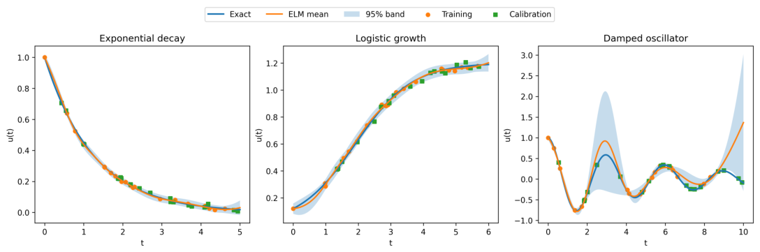
Figure 1 shows representative reconstructions for the three ODE classes using the conformalized ensemble ELM. The method tracks the exact trajectory closely for the monotone examples and remains calibrated for the oscillatory trajectory, where sparse observations make phase reconstruction more demanding. The uncertainty band widens in the nonlinear transition region of the logistic problem and around phase-sensitive portions of the damped oscillator.

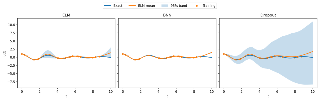
For the oscillatory problem, Figure 2 shows the qualitative difference among the three uncertainty mechanisms. The Bayesian random-feature interval is sharp but under-covers when the sparse data induce phase bias. The dropout interval is very wide in this capacity-matched implementation because mask-induced variability in oscillatory extrapolation is large. The conformalized ELM produces an intermediate band with coverage close to the nominal level and a much lower Winkler score.

5.3. Aggregate Calibration and Sharpness

The full metric summary is reported in

Table 1. Average performance over three independent random splits. Coverage probability (CP) is reported on the dense latent-state test grid at nominal level $0.95$. The table is resized to the text width to avoid boundary overflow.

Problem	Method	CP	AW	RMSE	Winkler
Damped oscillator	BNN	0.361 ± 0.078	0.094 ± 0.016	0.183 ± 0.116	2.813 ± 1.223
	Dropout	0.987 ± 0.022	9.204 ± 1.191	0.304 ± 0.127	9.231 ± 1.161
	ELM	0.952 ± 0.024	0.418 ± 0.181	0.179 ± 0.112	0.480 ± 0.241
Exponential decay	BNN	1.000 ± 0.000	0.085 ± 0.036	0.009 ± 0.002	0.085 ± 0.036
	Dropout	0.976 ± 0.036	0.334 ± 0.052	0.012 ± 0.003	0.342 ± 0.065
	ELM	0.987 ± 0.022	0.048 ± 0.005	0.009 ± 0.002	0.049 ± 0.006
Logistic growth	BNN	1.000 ± 0.000	0.079 ± 0.021	0.013 ± 0.003	0.079 ± 0.021
	Dropout	0.950 ± 0.025	0.366 ± 0.085	0.018 ± 0.004	0.370 ± 0.082
	ELM	0.983 ± 0.029	0.072 ± 0.015	0.013 ± 0.003	0.073 ± 0.014

. Coverage probability (CP) is computed on the dense latent-state test grid at nominal level $0.95$; AW is the average interval width; RMSE is the root mean squared error of the predictive mean; and the Winkler score rewards narrow intervals while penalizing missed coverage.

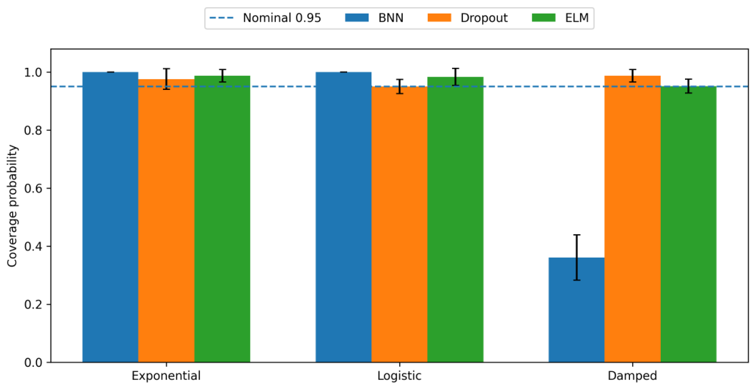
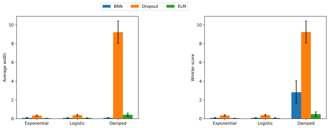
The conformalized ELM achieved CP values $0.987\pm 0.022$, $0.983\pm 0.029$, and $0.952\pm 0.024$ on the exponential, logistic, and damped-oscillator benchmarks, respectively. The first two values are mildly conservative, while the oscillatory value is close to the target. The Bayesian random-feature baseline is highly effective on the two smooth monotone examples, achieving CP equal to $1.000$ with competitive widths, but it under-covers on the oscillatory problem because the posterior variance is sharp relative to phase bias. The dropout baseline reaches or exceeds the nominal target in these experiments, while its widths are much larger, especially in the damped oscillator case. These results are consistent with the theory: model-based intervals can be sharp when the model captures the trajectory well, whereas conformal calibration directly corrects the empirical residual scale.

The coverage and sharpness trends are summarized visually in Figure 3 and Figure 4. Figure 3 shows the separation in empirical coverage. Figure 4 shows that the ELM intervals provide the lowest Winkler score on the exponential and damped-oscillator benchmarks and remain competitive on the logistic benchmark.

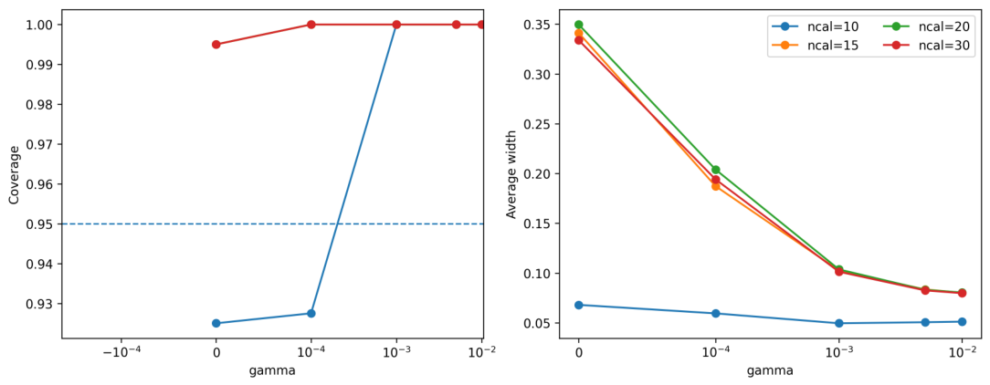
5.4. Denominator and Calibration-Size Ablation

To separate the influence of the denominator safeguard from the finite calibration split, we repeated the logistic-growth experiment for $\gamma \in \{0,{10}^{-4},{10}^{-3},5\times {10}^{-3},{10}^{-2}\}$ and $n_{\mathrm{cal}}\in \{10,15,20,30\}$. Figure 5 reports the resulting coverage and average width. With only $n_{\mathrm{cal}}=10$ calibration points, using $\gamma =0$ yielded CP $0.925$ and AW $0.068$, while $\gamma =5\times {10}^{-3}$ yielded CP $1.000$ and AW $0.051$. For $n_{\mathrm{cal}}=20$, the same change reduced AW from $0.350$ to $0.083$ while preserving CP at $0.995$–$1.000$. Thus the finite calibration quantile is the main source of discreteness and mild conservativeness, while the denominator safeguard regularizes small-spread calibration scores and prevents unstable interval inflation. Values between ${10}^{-3}$ and ${10}^{-2}$ produced similar conclusions in this benchmark.

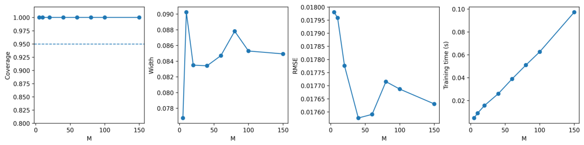
5.5. Ensemble-Size Sensitivity and Training Time

To examine the role of the ensemble size itself, we repeated the logistic experiment for

$$M\in \{5,10,20,40,60,80,100,150\}.$$

Figure 6 shows that the accuracy and interval metrics stabilize once the ensemble reaches moderate size. In the executed Python implementation, the measured ELM training-and-prediction time increased approximately linearly from $0.0048$ s at $M=5$ to $0.097$ s at $M=150$. The time at the main value $M=100$ was $0.063$ s for this split. This confirms that the additional ensemble members mainly add embarrassingly parallel ridge solves, while the calibration and evaluation steps remain inexpensive.

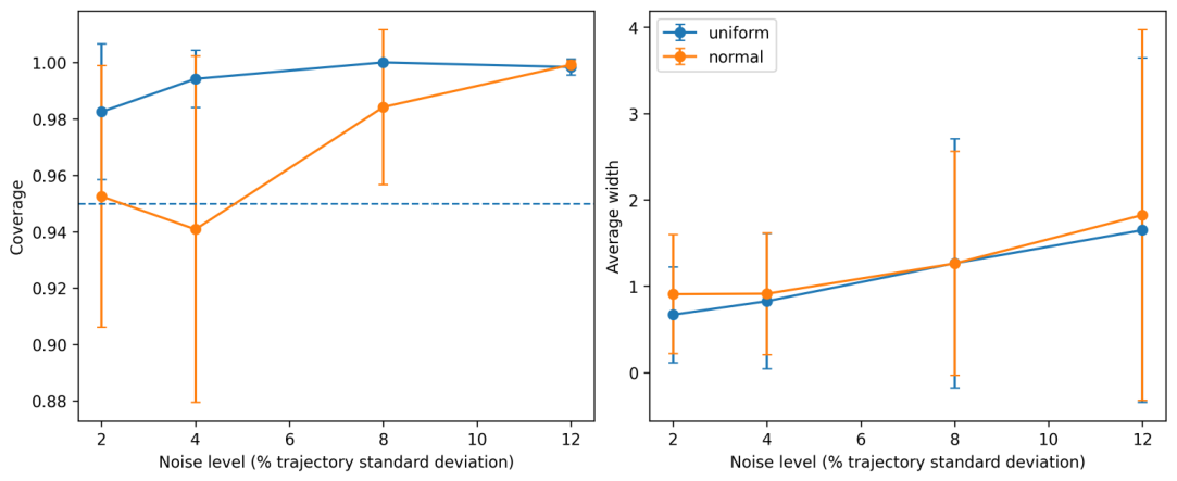
5.6. Noise Level and Hidden-Distribution Sensitivity

Figure 7 tests higher noise levels and the hidden-parameter distribution on the damped oscillator. The noise standard deviation was set to $2\%$, $4\%$, $8\%$, and $12\%$ of the trajectory standard deviation, and the hidden features were sampled either from the default uniform law or from the normal law stated in Section 2. Uniform sampling produced mean CP values $0.983$, $0.994$, $1.000$, and $0.998$ across the four noise levels, while normal sampling produced $0.953$, $0.941$, $0.984$, and $0.999$. The average widths increased with noise, as expected from calibration against noisier observations. This experiment verifies that the hidden-layer moment hypothesis used in Theorem 2 is compatible with the actual uniform and normal sampling schemes and that the method remains calibrated in substantially noisier regimes.

5.7. Limitations of the Numerical Study

The numerical study remains deliberately controlled. It uses scalar synthetic ODEs with known exact solutions, one-hidden-layer capacity-matched baselines, and three random splits for the aggregate table. The resulting evidence is therefore best interpreted as a focused validation of the coverage mechanism rather than as an exhaustive benchmark against every modern uncertainty-aware neural ODE architecture. In addition, the reported conformal bands are pointwise and marginal, exactly as in Theorem 3; simultaneous-in-time coverage would require a more conservative calibration rule. Finally, the ELM coverage in the monotone experiments is mildly conservative, which is useful for robustness in sparse settings and also motivates future work on adaptive safeguards and locally refined calibration rules to tighten the bands further.

6. Conclusions

This paper has introduced a conformalized ensemble extreme learning machine framework for uncertainty quantification in ordinary differential equations and has complemented the theory by an executed simulation study. The central mechanism is to train independently randomized ELM surrogates, use their ensemble mean as the reconstructed trajectory, and use the ensemble spread as a local uncertainty score. The resulting method preserves the main computational advantage of ELMs, namely, closed-form training of the output layer, while gaining a statistically meaningful uncertainty statement through split-conformal calibration.

The revised formulation makes explicit how the work differs from general ELM regression intervals and deep ensembles, specifies the hidden-layer sampling laws used in the experiments, verifies the finite-moment hypothesis for both uniform and normal sampling, clarifies the exchangeability condition behind the conformal theorem, and reports additional diagnostics for the denominator safeguard, calibration size, noise level, ensemble size, and training time.

The theoretical analysis established that each ensemble member satisfies the initial condition exactly, that the ensemble mean and spread are stable under perturbations of the response data, that the empirical spread converges almost surely to the random-feature predictive variance, and that the conformalized interval achieves finite-sample marginal coverage under exchangeability. The numerical study corroborated these statements in a concrete sparse-data regime. Across the exponential, logistic, and damped-oscillator benchmarks, the conformalized ensemble ELM attained near-nominal or mildly conservative pointwise coverage with competitive RMSE and favorable Winkler scores, especially on the phase-sensitive oscillatory example where model-based intervals can under-cover or become excessively wide.

For ODE trajectory reconstruction, these results place ensemble ELMs in a useful operating region: they are fast, parallel, mathematically transparent, and calibratable without committing to a fully correct probabilistic model. The most natural next steps are simultaneous-in-time bands, multivariate systems, adaptive random-feature distributions, block conformal calibration for serially dependent observations, and hybrid residual-penalized formulations that combine exact initial-condition enforcement with richer physics-informed structure.