Optimal Job Choice, Consumption, and Investment Under Subsistence-Consumption Constraints

Abstract

This paper extends a benchmark reversible job-choice framework by imposing a subsistence-consumption constraint. The agent chooses consumption, portfolio allocation, and one of two jobs in continuous time. The first job provides low income and high leisure, whereas the second job provides high income and low leisure. We focus on the case in which the coefficient of relative risk aversion satisfies $\gamma >1$, so that the transformed risk-aversion parameter also satisfies ${\gamma }_1>1$. Consumption must satisfy the lower bound $c_t\ge \underline{c}$ under both jobs. The constraint changes both the natural solvency boundary and the job-switching rule. In the dual problem, each job generates a subsistence-adjusted reward whose form depends on whether the consumption floor is binding. The optimal job is selected by the upper envelope of the two dual rewards. We prove that, when $\gamma >1$, the resulting dual switching function has a unique positive zero. We also characterize the location of this zero explicitly in terms of the income gap $Y_1-Y_0$ and the subsistence level $\underline{c}$. Hence the optimal job policy remains a one-threshold rule: the agent chooses the high-income job at low wealth and the high-leisure job at high wealth. The consumption floor shifts this boundary and implies that near the solvency boundary the agent necessarily consumes at the subsistence level and works in the high-income job. We provide a complete closed-form representation of the dual value function in all possible regimes.

1. Introduction

Since the seminal contributions of Merton [1,2], the continuous-time consumption–investment problem has served as a benchmark framework for analyzing intertemporal financial decisions under uncertainty. Subsequent studies have enriched this framework by incorporating labor income, labor-supply flexibility, and retirement decisions. For example, Bodie et al. [3] show that flexibility in labor supply can materially affect portfolio choice, while the optimal retirement literature studies how agents jointly determine consumption, investment, and labor-market exit decisions; see, among others, Choi and Shim [4], Choi et al. [5], Dybvig and Liu [6,7], Farhi and Panageas [8], Lim and Shin [9], Yang and Koo [10]. In these retirement models, however, labor-market exit is typically irreversible: once the agent retires, she cannot return to work.

A related but distinct strand of the literature studies reversible job choice. In the reversible setting, labor income is not merely an exogenous endowment, but an endogenous component of the agent’s decision problem. Shim and Shin [11] develop a continuous-time infinite-horizon model in which an agent chooses consumption, investment, and one of two reversible jobs under Cobb–Douglas consumption–leisure preferences. Their main result is a closed-form threshold policy: the agent works in the high-income/low-leisure job at low wealth and switches to the low-income/high-leisure job at high wealth. Shim et al. [12] extend this line of work by using a dynamic programming approach with labor disutility, and Lee et al. [13] analyze how borrowing constraints interact with effective labor-supply flexibility. More recent contributions consider additional labor-market frictions and life-cycle features, including retirement, switching costs, and finite horizons; see Jeon and Park [14], Jeon and Shim [15], Yang and Jeon [16]. In particular, Yang and Jeon [16] combine finite-horizon stochastic control with optimal switching under job-switching costs and a mandatory retirement date, leading to a system of parabolic variational inequalities and free-boundary problems.

The present paper focuses on another economically important friction: a subsistence-consumption requirement. Minimum consumption constraints are natural when consumption includes basic necessities such as housing, food, medical expenditure, and other non-discretionary expenses. They are also closely related to downside consumption constraints in portfolio choice. Gong and Li [17] study dynamic asset allocation with real subsistence consumption, Lakner and Ma Nygren [18] analyze portfolio optimization with downside constraints, and Mai et al. [19] consider voluntary retirement with consumption constraints. Closest to the present paper in economic motivation, Li et al. [20] study an optimal retirement problem with job switching, unemployment risk, and subsistence-consumption constraints. Their results show that unemployment risk and subsistence requirements can reduce consumption and investment before retirement. Li et al. [21] also emphasize that job-switching flexibility can interact with other long-run risks, such as inflation, mortality risk, and bequest motives, in shaping optimal consumption and investment behavior.

The empirical motivation for imposing a hard consumption floor is that a large part of household expenditure is non-discretionary. Housing, food, health care, commuting, and debt-service commitments cannot be reduced smoothly in response to adverse wealth shocks. Consistent with this view, empirical studies of consumption and labor supply emphasize that households use labor income and precautionary saving to buffer imperfectly insurable income and wealth risks; see, for example, Low [22], Blundell et al. [23], and Jappelli and Pistaferri [24]. In this respect, the unconstrained reversible job-choice benchmark may be counterfactual near the solvency boundary: it permits the agent to reduce consumption continuously without a lower bound, thereby weakening the need to remain in the high-income job. The subsistence constraint rules out this unrealistic adjustment margin and generates the prediction that low-wealth agents consume at the floor and choose the high-income job.

Table 1. Comparison with closely related models.

	Shim and Shin [11]	Li et al. [20]	This Paper
Reversible job choice	Yes	Yes	Yes
Subsistence-consumption floor	No	Yes	Yes
Retirement decision	No	Yes	No
Unemployment risk	No	Yes	No
Job-switching cost	No	No	No
Closed-form dual switching threshold	Yes	Not the main focus	Yes
Three-regime classification by the location of the floor	No	No	Yes
Complete coefficient-jump representation of the dual value	Yes, without floor	Not in this form	Yes
Main role in the literature	Benchmark reversible job choice	Richer retirement/unemployment environment	Tractable subsistence-adjusted benchmark

clarifies the intended contribution. Our objective is not to add all life-cycle risks considered in Li et al. [20]; rather, it is to isolate the subsistence-consumption channel in the canonical reversible job-choice model and to solve that benchmark in closed form. This separation allows us to show exactly when the unconstrained Shim–Shin threshold remains valid, when it must be replaced by a mixed binding–slack equation, and when the switching point lies in the region where the floor binds under both jobs.

The simplifying assumptions are therefore part of the benchmark design rather than claims of full realism. Stochastic labor income, non-constant leisure, job-specific expenditure needs, and costly job changes are important extensions. If labor income is stochastic but spanned by the traded asset, the martingale-duality method can still be written in terms of the state-price density and the present value of the stochastic income stream. If income contains a nonhedgeable component, however, the market becomes incomplete and the dual problem would involve a family of supermartingale deflators or equivalent martingale measures rather than a single density. Similarly, if switching between jobs entails a fixed cost, job choice is no longer a pointwise maximization of two dual rewards; it becomes a genuine optimal-switching problem with coupled variational inequalities. These extensions are mathematically meaningful, but they would obscure the main closed-form subsistence mechanism isolated in the present paper.

This paper extends a benchmark reversible job-choice framework by imposing a subsistence-consumption constraint. Specifically, for a fixed constant $\underline{c}>0$, admissible consumption must satisfy

$$c_t\ge \underline{c},t\ge 0.$$

This apparently simple constraint changes the structure of the problem in a substantial way. In the unconstrained model, the dual consumption demand under job $A_i$ is proportional to $z^{-1/{\gamma }_1}$, where z is the dual state variable. With a subsistence floor, the demand is truncated from below. Consequently, the dual reward associated with each job becomes piecewise, and the job-switching equation is no longer the unconstrained algebraic equation of Shim and Shin [11]. The natural solvency boundary also changes from the present value of the highest labor income to the present value of the cheapest feasible subsistence plan.

We formulate and solve the extended problem for the case $\gamma >1$. In this case

$${\gamma }_1:=1-\alpha (1-\gamma )>1,$$

and the leisure ordering implies a useful monotonic structure of the dual switching function. We show that the subsistence-adjusted switching function has exactly one positive zero. Thus the job-choice region remains simple, even though the dual value function is piecewise because the consumption floor can bind under neither job, one job, or both jobs. More precisely, the location of the switching point is determined by two critical income gaps, which separate the slack–slack, binding–slack, and binding–binding regimes.

Our contribution is threefold. First, we identify how a subsistence floor modifies the reversible job-choice threshold of Shim and Shin [11]. The unconstrained boundary remains valid only when it lies in the region where the floor is slack under both jobs. Otherwise, the switching equation must be replaced by a subsistence-adjusted equation. Second, we provide a full closed-form dual value function in all possible regimes. The solution is obtained by combining the martingale/duality method of Cox and Huang [25], Karatzas et al. [26], and Karatzas and Shreve [27] with explicit coefficient-jump formulas for the linear dual ordinary differential equation. Third, we translate the dual threshold into a primal wealth threshold and show that the optimal policy remains economically intuitive: the agent chooses the high-income job at low wealth and the high-leisure job at high wealth.

We also clarify the terminology used in the paper. Because job choice is reversible and costless, the dual problem does not generate an optimal-stopping or switching-cost variational inequality. The selected job is determined pointwise by the upper envelope $\mathsf{\Psi }\left(z\right)=max\{{\mathcal{U}}_0\left(z\right),{\mathcal{U}}_1\left(z\right)\}$, and the threshold $\widehat{z}$ is therefore an endogenous algebraic crossing point of two dual rewards. Thus, throughout the paper, we refer to $\widehat{z}$ and $\widehat{x}$ as switching thresholds or switching boundaries, not as free boundaries in the variational-inequality sense.

The economic implication is clear. Close to the solvency boundary, the shadow value of wealth is high and the consumption floor binds. Since consumption cannot be reduced below $\underline{c}$, the high-income job is strictly optimal in low-wealth states. At high wealth levels, the shadow value of income is low and the high-leisure job becomes optimal. Hence the subsistence constraint strengthens the precautionary motive for remaining in the high-income job and affects not only labor supply but also the shape of the consumption and portfolio rules near the switching boundary.

The remainder of the paper is organized as follows. Section 2 introduces the model and the subsistence-constrained admissible set. Section 3 derives the budget constraint and the dual problem. Section 4 analyzes the subsistence-adjusted switching function and characterizes the switching boundary. Section 5 provides the closed-form dual value function. Section 6, Section 7 and Section 8 recover the primal value function and optimal controls. Section 9 compares the constrained and unconstrained boundaries, Section 10 discusses numerical implications, and Section 11 concludes. For convenience, Appendix A collects the derivative formulas used to implement the marginal wealth relation and portfolio rule in the numerical analysis.

2. The Model

We consider a complete Black–Scholes financial market on a filtered probability space $(\mathsf{\Omega },\mathcal{F},{\left({\mathcal{F}}_t\right)}_{t\ge 0},\mathbb{P})$ supporting a standard Brownian motion B. The risk-free asset has constant interest rate $r>0$. The risky asset price satisfies

$${\displaystyle \frac{d{S}_t}{S_t}}=\mu dt+\sigma d{B}_t,\sigma >0,$$

(1)

where $\mu >r$. Define the market price of risk by

$$\theta :={\displaystyle \frac{\mu -r}{\sigma }}>0.$$

(2)

The agent chooses between two jobs $A_0$ and $A_1$. Job $A_i$ provides constant labor income $Y_i$ and constant leisure rate $L_i$. We assume

$$0\le Y_0<Y_1,0<L_1<L_0.$$

(3)

Thus $A_1$ is the high-income/low-leisure job, while $A_0$ is the low-income/high-leisure job.

Let ${\mathsf{\Theta }}_t\in \{A_0,A_1\}$ denote the job chosen at time t, let $c_t$ denote consumption, and let ${\pi }_t$ denote the dollar amount invested in the risky asset. The wealth process satisfies

$$d{X}_t=\left[r{X}_t+(\mu -r){\pi }_t-c_t+Y_0{\mathbf{1}}_{\{{\mathsf{\Theta }}_t=A_0\}}+Y_1{\mathbf{1}}_{\{{\mathsf{\Theta }}_t=A_1\}}\right]dt+\sigma {\pi }_{t}d{B}_t,X_0=x.$$

(4)

The agent has Cobb–Douglas consumption/leisure utility. We follow the transformation in Shim and Shin [11]. Let

$${\gamma }_1:=1-\alpha (1-\gamma ),0<\alpha <1.$$

(5)

Throughout the paper we impose the following restriction.

Assumption A1 

(Risk aversion). The coefficient of relative risk aversion satisfies

$$\gamma >1.$$

(6)

Consequently,

$${\gamma }_1=1+\alpha (\gamma -1)>1.$$

(7)

Moreover, since $0<\alpha <1$, we also have ${\gamma }_1<\gamma$.

Remark 1 

(Role of the restriction $\gamma >1$). The restriction $\gamma >1$ is both economically standard in quantitative consumption-portfolio models and technically central for the single-crossing result. Under this condition, ${\gamma }_1>1$ and ${\gamma }_1-\gamma <0$, so the leisure ordering $L_1<L_0$ implies $A_0<A_1$, $a_0<a_1$, and $m_0<m_1$. These strict inequalities make the derivative of the dual switching function monotone after the relevant transformation and yield the unique-crossing result in Lemma 2. Economically, $\gamma >1$ means that the agent is sufficiently risk averse that the marginal utility of subsistence consumption is high near the solvency boundary; this strengthens the preference for the high-income job in low-wealth states. Since job changes are costless in the present benchmark, the wealth process itself has no upward or downward jump at the switching boundary; only the selected job, consumption formula, and portfolio feedback may change across the boundary. If $\gamma <1$, the sign of $1-{\gamma }_1$ and the ordering of the transformed utility coefficients may change, and the dual switching function need not be single crossing. Conditional on a known ordering of crossing points, the coefficient-jump representation in Section 5 would still apply piece by piece, but the model may exhibit multiple switching intervals and no longer admits the one-threshold characterization of Section 4 and Section 5. We therefore focus on the economically relevant case $\gamma >1$, where the subsistence-adjusted threshold admits a complete closed-form characterization.

For job $A_i$, instantaneous utility from consumption is

$$U_i\left(c\right):=L_i^{{\gamma }_1-\gamma }{\displaystyle \frac{c^{1-{\gamma }_1}}{1-{\gamma }_1}},c>0,i=0,1.$$

(8)

Because ${\gamma }_1>1$, the denominator $1-{\gamma }_1$ is negative. The utility is increasing and strictly concave in c:

$$U_i^{\prime }\left(c\right)=L_i^{{\gamma }_1-\gamma }{c}^{-{\gamma }_1}>0,U_i^{\prime \prime }\left(c\right)=-{\gamma }_1{L}_i^{{\gamma }_1-\gamma }{c}^{-{\gamma }_1-1}<0.$$

The new constraint is the subsistence requirement

$$c_t\ge \underline{c}>0,t\ge 0.$$

(9)

Remark 2 

(Job-specific floors and switching costs). The common floor $\underline{c}$ is imposed to keep the benchmark analytically transparent. If job $A_i$ instead required a deterministic job-specific floor ${\underline{c}}_i$, for example because commuting, location, or work-related expenses differ across jobs, the pointwise dual reward would become

$${\mathcal{U}}_i(z;{\underline{c}}_i)=\underset{c\ge {\underline{c}}_i}{sup}\{U_i\left(c\right)-zc+Y_{i}z\}.$$

For deterministic work-related expenses, one may equivalently reinterpret $Y_i$ as net labor income and ${\underline{c}}_i$ as the residual minimum consumption requirement. The closed-form formulas would then remain piecewise but would involve the two thresholds $A_i{\underline{c}}_i^{-{\gamma }_1}$. By contrast, a fixed cost paid at each job change cannot be absorbed into $Y_i$ or ${\underline{c}}_i$; it would replace the pointwise envelope $max\{{\mathcal{U}}_0,{\mathcal{U}}_1\}$ by a genuine optimal-switching problem with intervention costs. We leave that costly switching extension for future work.

Since the agent can always choose the high-income job $A_1$ and consume the minimum amount $\underline{c}$, the natural solvency boundary is

$$\underline{x}:={\displaystyle \frac{\underline{c}-Y_1}{r}}=-{\displaystyle \frac{Y_1-\underline{c}}{r}}.$$

(10)

Indeed, if the agent chooses $A_1$ forever and consumes $\underline{c}$ forever, the present value of net consumption is $(\underline{c}-Y_1)/r$. Therefore the admissible wealth region is

$$x>\underline{x}.$$

(11)

The boundary $\underline{x}$ can be negative, zero, or positive depending on whether $Y_1$ is larger than, equal to, or smaller than $\underline{c}$. In particular, if $X_0=\underline{x}$ and the agent chooses $A_1$, consumes $c_t=\underline{c}$, and sets ${\pi }_t=0$, then the drift in (4) is zero and the wealth process remains constant at $\underline{x}$. Equivalently, since $\mathbb{E}\left[H_t\right]=e^{-rt}$, the state-price present value of the net subsistence expenditure generated by this plan is

$$\mathbb{E}\left[{\int }_0^{\infty }{H}_t(\underline{c}-Y_1)dt\right]=(\underline{c}-Y_1){\int }_0^{\infty }{e}^{-rt}dt={\displaystyle \frac{\underline{c}-Y_1}{r}}.$$

Thus an initial wealth below $\underline{x}$ cannot finance the cheapest feasible subsistence plan, while $x=\underline{x}$ can finance it exactly. This confirms that (10) is the natural solvency boundary.

Definition 1 

(Admissible controls). For $x>\underline{x}$, a control triple $(\mathsf{\Theta },c,\pi )$ is admissible if the following conditions hold:

(i)

Θ is progressively measurable and takes values in $\{A_0,A_1\}$;

(ii)

c is progressively measurable, $c_t\ge \underline{c}$ for all $t\ge 0$, and ${\int }_0^t{c}_{s}ds<\infty$ a.s. for all $t\ge 0$;

(iii)

π is progressively measurable and ${\int }_0^t{\pi }_s^{2}ds<\infty$ a.s. for all $t\ge 0$;

(iv)

the wealth process in (4) satisfies

$$X_t\ge \underline{x},t\ge 0,$$

almost surely.

The set of all admissible controls is denoted by ${\mathcal{A}}_{\underline{c}}\left(x\right)$.

The agent maximizes

$$J(x;\mathsf{\Theta },c,\pi ):=\mathbb{E}\left[{\int }_0^{\infty }{e}^{-\rho t}\left(U_0\left(c_t\right){\mathbf{1}}_{\{{\mathsf{\Theta }}_t=A_0\}}+U_1\left(c_t\right){\mathbf{1}}_{\{{\mathsf{\Theta }}_t=A_1\}}\right)dt\right],$$

(12)

where $\rho >0$ is the subjective discount rate. The infinite-horizon discounted objective and the stationary notation follow the reversible job-choice formulation of Shim and Shin [11]; the new ingredient is the admissibility restriction $c_t\ge \underline{c}$. The value function is

$$V\left(x\right):=\underset{(\mathsf{\Theta },c,\pi )\in {\mathcal{A}}_{\underline{c}}\left(x\right)}{sup}J(x;\mathsf{\Theta },c,\pi ),x>\underline{x}.$$

(13)

Assumption 2 

(Finiteness). The parameters satisfy

$$K_1:=r+{\displaystyle \frac{\rho -r}{{\gamma }_1}}+{\displaystyle \frac{{\gamma }_1-1}{2{\gamma }_1^2}}{\theta }^2>0.$$

(14)

This is the standard finiteness condition for the unconstrained Merton component. It is the same condition that appears in the unconstrained dual formulation of Shim and Shin [11], with the transformed risk-aversion parameter ${\gamma }_1$. It guarantees that the power term in the dual value is finite.

3. Budget Constraint and the Dual Problem

The state-price density is

$$H_t:=exp\left(-\left(r+{\displaystyle \frac{1}{2}}{\theta }^2\right)t-\theta B_t\right).$$

(15)

For any admissible policy, the standard budget inequality is

$$\mathbb{E}\left[{\int }_0^{\infty }{H}_t\left(c_t-Y_0{\mathbf{1}}_{\{{\mathsf{\Theta }}_t=A_0\}}-Y_1{\mathbf{1}}_{\{{\mathsf{\Theta }}_t=A_1\}}\right)dt\right]\le x.$$

(16)

The solvency boundary (10) is the lower bound associated with the cheapest feasible subsistence plan, namely choosing $A_1$ and consuming $\underline{c}$ forever.

The dual notation in this section follows the martingale-duality reduction used in Shim and Shin [11]. The only change is that the pointwise Fenchel transform is now taken over $c\ge \underline{c}$, which creates the piecewise dual reward below.

For $z>0$, define the subsistence-adjusted dual reward associated with job $A_i$ by

$${\mathcal{U}}_i\left(z\right):=\underset{c\ge \underline{c}}{sup}\{U_i\left(c\right)-zc+Y_{i}z\}.$$

(17)

We introduce the notation

$$A_i:=L_i^{{\gamma }_1-\gamma },a_i:=A_i^{1/{\gamma }_1}=L_i^{({\gamma }_1-\gamma )/{\gamma }_1},m_i:=A_i{\underline{c}}^{-{\gamma }_1}.$$

(18)

Since $\gamma >1$, we have

$${\gamma }_1-\gamma =(1-\alpha )(1-\gamma )<0.$$

(19)

Together with $L_1<L_0$, this implies

$$0<A_0<A_1,0<a_0<a_1,0<m_0<m_1.$$

(20)

Thus the high-leisure job $A_0$ has a lower coefficient $A_0$ in the transformed utility representation because the denominator in (8) is negative. All inequalities in (20) are strict because $L_1<L_0$ and the exponent ${\gamma }_1-\gamma$ is strictly negative.

Lemma 1 

(Pointwise constrained consumption). For each job $A_i$, the maximizer in (17) is

$$c_i\left(z\right)=max\{\underline{c},a_i{z}^{-1/{\gamma }_1}\}.$$

(21)

Equivalently,

$$c_i\left(z\right)=a_i{z}^{-1/{\gamma }_1}\mathrm{if}0<z\le m_i,c_i\left(z\right)=\underline{c}\mathrm{if}z>m_i.$$

(22)

Moreover,

$${\mathcal{U}}_i\left(z\right)=\left\{\begin{array}{cc}{\displaystyle \frac{{\gamma }_1}{1-{\gamma }_1}{a}_i{z}^{\frac{{\gamma }_1-1}{{\gamma }_1}}+Y_{i}z,}\hfill & 0<z\le m_i,\hfill \\ {\displaystyle \frac{A_i}{1-{\gamma }_1}{\underline{c}}^{1-{\gamma }_1}+(Y_i-\underline{c})z,}\hfill & z>m_i.\hfill \end{array}\right.$$

(23)

Proof. 

For fixed i, the map $c\mapsto U_i\left(c\right)-zc$ is strictly concave on $(0,\infty )$. The derivative of the unconstrained objective is

$${\displaystyle \frac{\partial }{\partial c}}\{U_i\left(c\right)-zc\}=A_i{c}^{-{\gamma }_1}-z.$$

Setting this derivative equal to zero gives $A_i{c}^{-{\gamma }_1}=z$, or equivalently $c=A_i^{1/{\gamma }_1}{z}^{-1/{\gamma }_1}=a_i{z}^{-1/{\gamma }_1}$. Imposing $c\ge \underline{c}$ gives (21). If $a_i{z}^{-1/{\gamma }_1}\ge \underline{c}$, equivalently $z\le A_i{\underline{c}}^{-{\gamma }_1}=m_i$, the floor is slack. Otherwise the floor binds. Substituting these two cases into (17) gives (23). □

The dual job-selection payoff is the upper envelope

$$\mathsf{\Psi }\left(z\right):=max\{{\mathcal{U}}_0\left(z\right),{\mathcal{U}}_1\left(z\right)\},z>0.$$

(24)

Define the switching function

$${\Delta }_{\underline{c}}\left(z\right):={\mathcal{U}}_0\left(z\right)-{\mathcal{U}}_1\left(z\right).$$

(25)

Then the pointwise optimal job in the dual problem is

$$j^{*}\left(z\right)=\left\{\begin{array}{cc}0,\hfill & {\Delta }_{\underline{c}}\left(z\right)\ge 0,\hfill \\ 1,\hfill & {\Delta }_{\underline{c}}\left(z\right)<0.\hfill \end{array}\right.$$

(26)

At a point where ${\Delta }_{\underline{c}}\left(z\right)=0$, both jobs give the same instantaneous dual reward.

4. The Subsistence-Adjusted Switching Function

Because $0<m_0<m_1$, the explicit form of ${\Delta }_{\underline{c}}$ has three regimes:

$${\Delta }_{\underline{c}}\left(z\right)=\left\{\begin{array}{cc}{\displaystyle \frac{{\gamma }_1}{1-{\gamma }_1}(a_0-a_1)z^{\frac{{\gamma }_1-1}{{\gamma }_1}}+(Y_0-Y_1)z,}\hfill & 0<z\le m_0,\hfill \\ {\displaystyle \frac{A_0}{1-{\gamma }_1}{\underline{c}}^{1-{\gamma }_1}-\frac{{\gamma }_1}{1-{\gamma }_1}{a}_1{z}^{\frac{{\gamma }_1-1}{{\gamma }_1}}+(Y_0-Y_1-\underline{c})z,}\hfill & m_0<z\le m_1,\hfill \\ {\displaystyle \frac{A_0-A_1}{1-{\gamma }_1}{\underline{c}}^{1-{\gamma }_1}+(Y_0-Y_1)z,}\hfill & z>m_1.\hfill \end{array}\right.$$

(27)

The first region is the region in which the floor is slack under both jobs. The second region is the region in which the floor binds under the high-leisure job $A_0$ but remains slack under the high-income job $A_1$. The third region is the region in which the floor binds under both jobs.

Lemma 2 

(Single crossing of the dual job payoff). Under Assumption 1 and the ordering (3), the switching function ${\Delta }_{\underline{c}}$ has a unique positive zero. More precisely, there exists a unique $\widehat{z}\in (0,\infty )$ such that

$${\Delta }_{\underline{c}}\left(\widehat{z}\right)=0,$$

(28)

and

$${\Delta }_{\underline{c}}\left(z\right)>0\mathrm{for}0<z<\widehat{z},{\Delta }_{\underline{c}}\left(z\right)<0\mathrm{for}z>\widehat{z}.$$

(29)

Proof. 

By the envelope theorem applied to (17),

$${\mathcal{U}}_i^{\prime }\left(z\right)=Y_i-c_i\left(z\right)$$

(30)

at all points where the derivative exists. Since $c_i$ is continuous at $m_i$, ${\mathcal{U}}_i$ is continuously differentiable. Hence

$${\Delta }_{\underline{c}}^{\prime }\left(z\right)=Y_0-Y_1-c_0\left(z\right)+c_1\left(z\right).$$

(31)

Using $0<m_0<m_1$, we obtain

$${\Delta }_{\underline{c}}^{\prime }\left(z\right)=\left\{\begin{array}{cc}{\displaystyle Y_0-Y_1+(a_1-a_0)z^{-1/{\gamma }_1},}\hfill & 0<z<m_0,\hfill \\ {\displaystyle Y_0-Y_1-\underline{c}+a_1{z}^{-1/{\gamma }_1},}\hfill & m_0<z<m_1,\hfill \\ {\displaystyle Y_0-Y_1,}\hfill & z>m_1.\hfill \end{array}\right.$$

(32)

The derivative is continuous at $m_0$ and $m_1$ because $a_i{m}_i^{-1/{\gamma }_1}=\underline{c}$. Moreover, it is strictly decreasing on $(0,m_1)$ and equals the negative constant $Y_0-Y_1<0$ on $(m_1,\infty )$. Also,

$$\underset{z\downarrow 0}{lim}{\Delta }_{\underline{c}}\left(z\right)=0,\underset{z\downarrow 0}{lim}{\Delta }_{\underline{c}}^{\prime }\left(z\right)=+\infty ,$$

so ${\Delta }_{\underline{c}}\left(z\right)>0$ for all sufficiently small $z>0$. On the other hand, for $z>m_1$,

$${\Delta }_{\underline{c}}\left(z\right)={\displaystyle \frac{A_0-A_1}{1-{\gamma }_1}}{\underline{c}}^{1-{\gamma }_1}-(Y_1-Y_0)z⟶-\infty \mathrm{as}z\to \infty .$$

Therefore at least one positive zero exists.

It remains to prove uniqueness. Since ${\Delta }_{\underline{c}}^{\prime }$ is nonincreasing on $(0,\infty )$, once ${\Delta }_{\underline{c}}^{\prime }$ becomes nonpositive, ${\Delta }_{\underline{c}}$ is nonincreasing forever. Before that point ${\Delta }_{\underline{c}}$ is increasing and, as shown above, it is positive near zero. Hence ${\Delta }_{\underline{c}}$ cannot cross zero before its maximum. After its maximum, it is strictly decreasing until it reaches the linear tail and then remains strictly decreasing. Since it tends to $-\infty$, it crosses zero exactly once. This proves (29). □

Proposition 1 

(Regime-specific switching equation). The unique root $\widehat{z}$ is determined by exactly one of the following equations:

$$\begin{array}{cccc}\hfill & {\displaystyle \frac{{\gamma }_1}{1-{\gamma }_1}}(a_0-a_1)z^{\frac{{\gamma }_1-1}{{\gamma }_1}}+(Y_0-Y_1)z=0,\hfill & \hfill & 0<z\le m_0,\hfill \end{array}$$

(33)

$$\begin{array}{cccc}\hfill & {\displaystyle \frac{A_0}{1-{\gamma }_1}}{\underline{c}}^{1-{\gamma }_1}-{\displaystyle \frac{{\gamma }_1}{1-{\gamma }_1}}{a}_1{z}^{\frac{{\gamma }_1-1}{{\gamma }_1}}+(Y_0-Y_1-\underline{c})z=0,\hfill & \hfill & m_0<z\le m_1,\hfill \end{array}$$

(34)

$$\begin{array}{cccc}\hfill & {\displaystyle \frac{A_0-A_1}{1-{\gamma }_1}}{\underline{c}}^{1-{\gamma }_1}+(Y_0-Y_1)z=0,\hfill & \hfill & z>m_1.\hfill \end{array}$$

(35)

In the first and third regimes, the candidate roots are explicit:

$$\begin{array}{cc}\hfill z_{uu}& ={\left({\displaystyle \frac{{\gamma }_1(a_1-a_0)}{({\gamma }_1-1)(Y_1-Y_0)}}\right)}^{{\gamma }_1},\hfill \end{array}$$

(36)

$$\begin{array}{cc}\hfill z_{bb}& ={\displaystyle \frac{A_1-A_0}{({\gamma }_1-1)(Y_1-Y_0)}}{\underline{c}}^{1-{\gamma }_1}.\hfill \end{array}$$

(37)

Thus $\widehat{z}=z_{uu}$ if $z_{uu}\le m_0$, while $\widehat{z}=z_{bb}$ if $z_{bb}\ge m_1$. Otherwise $\widehat{z}$ is the unique solution of (34) in $(m_0,m_1)$.

Proof. 

The three equations are exactly the three pieces of (27). Lemma 2 guarantees that only one of these regime-consistent roots can be the true root. Solving (33) gives (36); solving the linear Equation (35) gives (37). If neither explicit candidate is regime-consistent, the unique zero must lie in the intermediate interval $(m_0,m_1)$ and is therefore characterized by (34). □

Proposition 2 

(Location of the dual switching boundary). Let

$$\delta :=Y_1-Y_0>0,\eta :={\displaystyle \frac{{\gamma }_1-1}{{\gamma }_1}}\in (0,1).$$

(38)

Define two critical income gaps by

$${\delta }_b:={\displaystyle \frac{\underline{c}}{{\gamma }_1-1}}\left(1-{\displaystyle \frac{A_0}{A_1}}\right),{\delta }_u:={\displaystyle \frac{{\gamma }_1\underline{c}}{{\gamma }_1-1}}\left({\displaystyle \frac{a_1-a_0}{a_0}}\right).$$

(39)

Then

$$0<{\delta }_b<{\delta }_u.$$

(40)

The unique dual switching boundary $\widehat{z}$ is characterized as follows.

(i) 

If $\delta \ge {\delta }_u$, then $\widehat{z}\le m_0$ and

$$\widehat{z}={\left[{\displaystyle \frac{{\gamma }_1(a_1-a_0)}{({\gamma }_1-1)\delta }}\right]}^{{\gamma }_1}.$$

(41)

In this case, the switching boundary lies in the region where the subsistence constraint is slack under both jobs.

(ii) 

If ${\delta }_b<\delta <{\delta }_u$, then

$$m_0<\widehat{z}<m_1,$$

(42)

and $\widehat{z}$ is the unique solution on $(m_0,m_1)$ of

$$-{\displaystyle \frac{A_0}{{\gamma }_1-1}}{\underline{c}}^{1-{\gamma }_1}+{\displaystyle \frac{{\gamma }_1}{{\gamma }_1-1}}{a}_1{z}^{\eta }-(\delta +\underline{c})z=0.$$

(43)

In this case, the subsistence constraint binds under job $A_0$ but remains slack under job $A_1$ at the switching boundary.

(iii) 

If $0<\delta \le {\delta }_b$, then $\widehat{z}\ge m_1$ and

$$\widehat{z}={\displaystyle \frac{A_1-A_0}{({\gamma }_1-1)\delta }}{\underline{c}}^{1-{\gamma }_1}.$$

(44)

In this case, the switching boundary lies in the region where the subsistence constraint binds under both jobs.

Proof. 

We already know from (20) that $A_0<A_1$, $a_0<a_1$, and $m_0<m_1$. Therefore ${\delta }_b>0$ and ${\delta }_u>0$.

Consider first the slack–slack candidate root $z_{uu}$ in (36). Since

$$m_0=A_0{\underline{c}}^{-{\gamma }_1}=a_0^{{\gamma }_1}{\underline{c}}^{-{\gamma }_1}={\left({\displaystyle \frac{a_0}{\underline{c}}}\right)}^{{\gamma }_1},$$

the condition $z_{uu}\le m_0$ is equivalent to

$${\displaystyle \frac{{\gamma }_1(a_1-a_0)}{({\gamma }_1-1)\delta }}\le {\displaystyle \frac{a_0}{\underline{c}}}.$$

Equivalently,

$$\delta \ge {\displaystyle \frac{{\gamma }_1\underline{c}}{{\gamma }_1-1}}\left({\displaystyle \frac{a_1-a_0}{a_0}}\right)={\delta }_u.$$

This proves part (i).

Next consider the binding–binding candidate root $z_{bb}$ in (37). Since

$$m_1=A_1{\underline{c}}^{-{\gamma }_1},$$

the condition $z_{bb}\ge m_1$ is equivalent to

$${\displaystyle \frac{A_1-A_0}{({\gamma }_1-1)\delta }}{\underline{c}}^{1-{\gamma }_1}\ge A_1{\underline{c}}^{-{\gamma }_1}.$$

Equivalently,

$$\delta \le {\displaystyle \frac{\underline{c}}{{\gamma }_1-1}}\left(1-{\displaystyle \frac{A_0}{A_1}}\right)={\delta }_b.$$

This proves part (iii).

If ${\delta }_b<\delta <{\delta }_u$, then neither explicit candidate lies in its own admissible regime. By Lemma 2, the unique root must therefore lie in the only remaining interval, namely $(m_0,m_1)$. On that interval, Equation (27) reduces to (43). This proves part (ii).

It remains to verify (40). Put $q:=a_1/a_0>1$. Since $A_1/A_0=q^{{\gamma }_1}$, we have

$${\delta }_b={\displaystyle \frac{\underline{c}}{{\gamma }_1-1}}\left(1-q^{-{\gamma }_1}\right),{\delta }_u={\displaystyle \frac{{\gamma }_1\underline{c}}{{\gamma }_1-1}}(q-1).$$

The inequality

$$1-q^{-{\gamma }_1}<{\gamma }_1(q-1)$$

holds for every $q>1$ and ${\gamma }_1>1$. Indeed, define $h\left(q\right):={\gamma }_1(q-1)-1+q^{-{\gamma }_1}$. Then $h\left(1\right)=0$ and

$$h^{\prime }\left(q\right)={\gamma }_1\left(1-q^{-{\gamma }_1-1}\right)>0$$

for all $q>1$. Hence ${\delta }_b<{\delta }_u$. □

The subsistence-adjusted upper envelope is therefore

$$\mathsf{\Psi }\left(z\right)=\left\{\begin{array}{cc}{\mathcal{U}}_0\left(z\right),\hfill & 0<z\le \widehat{z},\hfill \\ {\mathcal{U}}_1\left(z\right),\hfill & z>\widehat{z}.\hfill \end{array}\right.$$

(45)

Combining (23) and (45) gives the exact form of the dual running payoff.

5. The Dual Value Function

• For $z>0$, define the dual state process

  $$Z_t^z:=z{e}^{\rho t}{H}_t=zexp\left(\left(\rho -r-{\displaystyle \frac{1}{2}}{\theta }^2\right)t-\theta B_t\right).$$

  (46)

Then

$${\displaystyle \frac{d{Z}_t^z}{Z_t^z}}=(\rho -r)dt-\theta d{B}_t,Z_0^z=z.$$

(47)

The dual value function is

$$v\left(z\right):=\mathbb{E}\left[{\int }_0^{\infty }{e}^{-\rho t}\mathsf{\Psi }\left(Z_t^z\right)dt\right].$$

(48)

Let

$$f\left(n\right):={\displaystyle \frac{1}{2}}{\theta }^2{n}^2+\left(\rho -r-{\displaystyle \frac{1}{2}}{\theta }^2\right)n-\rho .$$

(49)

The two roots of $f\left(n\right)=0$ are denoted by

$$n_{+}>1,n_{-}<0.$$

(50)

The infinitesimal operator associated with Z and discounting is

$${\mathcal{L}}_{Z}v\left(z\right):={\displaystyle \frac{1}{2}}{\theta }^2{z}^2{v}^{\prime \prime }\left(z\right)+(\rho -r)z{v}^{\prime }\left(z\right)-\rho v\left(z\right).$$

(51)

The dual value solves

$${\mathcal{L}}_{Z}v\left(z\right)+\mathsf{\Psi }\left(z\right)=0,z>0.$$

(52)

5.1. Particular Solutions

Recall from (38) that $\eta =({\gamma }_1-1)/{\gamma }_1\in (0,1)$. If job $A_i$ is selected and the floor is slack, the running payoff is

$${\displaystyle \frac{{\gamma }_1}{1-{\gamma }_1}}{a}_i{z}^{\eta }+Y_{i}z.$$

A particular solution of (52) is

$${\mathsf{\Phi }}_i^u\left(z\right):={\displaystyle \frac{{\gamma }_1{a}_i}{(1-{\gamma }_1)K_1}}{z}^{\eta }+{\displaystyle \frac{Y_i}{r}}z.$$

(53)

Indeed, Assumption 2 gives

$$f\left(\eta \right)=-K_1.$$

If job $A_i$ is selected and the floor binds, the running payoff is

$${\displaystyle \frac{A_i}{1-{\gamma }_1}}{\underline{c}}^{1-{\gamma }_1}+(Y_i-\underline{c})z.$$

A particular solution is

$${\mathsf{\Phi }}_i^b\left(z\right):={\displaystyle \frac{A_i}{\rho (1-{\gamma }_1)}}{\underline{c}}^{1-{\gamma }_1}+{\displaystyle \frac{Y_i-\underline{c}}{r}}z.$$

(54)

For later use, set

$${\mathsf{\Phi }}_{0u}:={\mathsf{\Phi }}_0^u,{\mathsf{\Phi }}_{0b}:={\mathsf{\Phi }}_0^b,{\mathsf{\Phi }}_{1u}:={\mathsf{\Phi }}_1^u,{\mathsf{\Phi }}_{1b}:={\mathsf{\Phi }}_1^b.$$

(55)

5.2. Closed-Form Dual Value Function

We now give the closed-form expression of the dual value function. Set

$$p:=n_{+},q:=n_{-}.$$

(56)

For two regimes $R,S\in \{0u,0b,1u,1b\}$ and a transition point $\beta >0$, define

$$A_{R,S}\left(\beta \right):={\mathsf{\Phi }}_R\left(\beta \right)-{\mathsf{\Phi }}_S\left(\beta \right),$$

(57)

and

$$B_{R,S}\left(\beta \right):={\mathsf{\Phi }}_R^{\prime }\left(\beta \right)-{\mathsf{\Phi }}_S^{\prime }\left(\beta \right).$$

(58)

The jump in the homogeneous coefficients caused by changing the particular solution from ${\mathsf{\Phi }}_R$ to ${\mathsf{\Phi }}_S$ at $\beta$ is

$$d_{R,S}^{+}\left(\beta \right):={\displaystyle \frac{\beta B_{R,S}\left(\beta \right)-q{A}_{R,S}\left(\beta \right)}{(p-q){\beta }^p}},$$

(59)

and

$$d_{R,S}^{-}\left(\beta \right):={\displaystyle \frac{p{A}_{R,S}\left(\beta \right)-\beta B_{R,S}\left(\beta \right)}{(p-q){\beta }^q}}.$$

(60)

Indeed, if

$$v^{-}\left(z\right)=C_{-}^{+}{z}^p+C_{-}^{-}{z}^q+{\mathsf{\Phi }}_R\left(z\right)$$

on the left of $\beta$, and

$$v^{+}\left(z\right)=C_{+}^{+}{z}^p+C_{+}^{-}{z}^q+{\mathsf{\Phi }}_S\left(z\right)$$

on the right of $\beta$, then value matching and smooth matching imply

$$C_{+}^{+}-C_{-}^{+}=d_{R,S}^{+}\left(\beta \right),C_{+}^{-}-C_{-}^{-}=d_{R,S}^{-}\left(\beta \right).$$

(61)

Derivation of (59) and (60). The matching conditions at $\beta$ are

$$(C_{+}^{+}-C_{-}^{+}){\beta }^p+(C_{+}^{-}-C_{-}^{-}){\beta }^q=A_{R,S}\left(\beta \right),$$

and

$$p(C_{+}^{+}-C_{-}^{+}){\beta }^{p-1}+q(C_{+}^{-}-C_{-}^{-}){\beta }^{q-1}=B_{R,S}\left(\beta \right).$$

Multiplying the second equation by $\beta$ and solving the resulting two-by-two linear system gives (59) and (60). □

We distinguish the three possible locations of the switching point $\widehat{z}$.

• Case I: $\widehat{z}\le m_0$.

This case occurs when $Y_1-Y_0\ge {\delta }_u$. The relevant regimes are

$$0u⟶1u⟶1b,$$

with transition points $\widehat{z}$ and $m_1$. Define

$$d_1^{\pm }:=d_{0u,1u}^{\pm }\left(\widehat{z}\right),d_2^{\pm }:=d_{1u,1b}^{\pm }\left(m_1\right).$$

(62)

Then the dual value function is

$$v\left(z\right)=\left\{\begin{array}{cc}{\displaystyle C_0^{+}{z}^p+{\mathsf{\Phi }}_{0u}\left(z\right),}\hfill & 0<z\le \widehat{z},\hfill \\ {\displaystyle C_1^{+}{z}^p+C_1^{-}{z}^q+{\mathsf{\Phi }}_{1u}\left(z\right),}\hfill & \widehat{z}<z\le m_1,\hfill \\ {\displaystyle C_2^{-}{z}^q+{\mathsf{\Phi }}_{1b}\left(z\right),}\hfill & z>m_1,\hfill \end{array}\right.$$

(63)

where

$$C_0^{+}=-(d_1^{+}+d_2^{+}),C_1^{+}=-d_2^{+},C_1^{-}=d_1^{-},C_2^{-}=d_1^{-}+d_2^{-}.$$

(64)

The terms $C_0^{-}{z}^q$ and $C_2^{+}{z}^p$ are absent because the growth conditions at zero and infinity require $C_0^{-}=0$ and $C_2^{+}=0$.

• Case II: $m_0<\widehat{z}<m_1$.

This case occurs when ${\delta }_b<Y_1-Y_0<{\delta }_u$. The relevant regimes are

$$0u⟶0b⟶1u⟶1b,$$

with transition points $m_0$, $\widehat{z}$, and $m_1$. Define

$$d_1^{\pm }:=d_{0u,0b}^{\pm }\left(m_0\right),d_2^{\pm }:=d_{0b,1u}^{\pm }\left(\widehat{z}\right),d_3^{\pm }:=d_{1u,1b}^{\pm }\left(m_1\right).$$

(65)

Then the dual value function is

$$v\left(z\right)=\left\{\begin{array}{cc}{\displaystyle C_0^{+}{z}^p+{\mathsf{\Phi }}_{0u}\left(z\right),}\hfill & 0<z\le m_0,\hfill \\ {\displaystyle C_1^{+}{z}^p+C_1^{-}{z}^q+{\mathsf{\Phi }}_{0b}\left(z\right),}\hfill & m_0<z\le \widehat{z},\hfill \\ {\displaystyle C_2^{+}{z}^p+C_2^{-}{z}^q+{\mathsf{\Phi }}_{1u}\left(z\right),}\hfill & \widehat{z}<z\le m_1,\hfill \\ {\displaystyle C_3^{-}{z}^q+{\mathsf{\Phi }}_{1b}\left(z\right),}\hfill & z>m_1,\hfill \end{array}\right.$$

(66)

where

$$C_0^{+}=-(d_1^{+}+d_2^{+}+d_3^{+}),$$

(67)

$$C_1^{+}=-(d_2^{+}+d_3^{+}),C_1^{-}=d_1^{-},$$

(68)

$$C_2^{+}=-d_3^{+},C_2^{-}=d_1^{-}+d_2^{-},$$

(69)

and

$$C_3^{-}=d_1^{-}+d_2^{-}+d_3^{-}.$$

(70)

Again $C_0^{-}=0$ and $C_3^{+}=0$ by the boundary growth conditions.

• Case III: $\widehat{z}\ge m_1$.

This case occurs when $0<Y_1-Y_0\le {\delta }_b$. The relevant regimes are

$$0u⟶0b⟶1b,$$

with transition points $m_0$ and $\widehat{z}$. Define

$$d_1^{\pm }:=d_{0u,0b}^{\pm }\left(m_0\right),d_2^{\pm }:=d_{0b,1b}^{\pm }\left(\widehat{z}\right).$$

(71)

Then the dual value function is

$$v\left(z\right)=\left\{\begin{array}{cc}{\displaystyle C_0^{+}{z}^p+{\mathsf{\Phi }}_{0u}\left(z\right),}\hfill & 0<z\le m_0,\hfill \\ {\displaystyle C_1^{+}{z}^p+C_1^{-}{z}^q+{\mathsf{\Phi }}_{0b}\left(z\right),}\hfill & m_0<z\le \widehat{z},\hfill \\ {\displaystyle C_2^{-}{z}^q+{\mathsf{\Phi }}_{1b}\left(z\right),}\hfill & z>\widehat{z},\hfill \end{array}\right.$$

(72)

where

$$C_0^{+}=-(d_1^{+}+d_2^{+}),C_1^{+}=-d_2^{+},C_1^{-}=d_1^{-},C_2^{-}=d_1^{-}+d_2^{-}.$$

(73)

The growth restrictions again impose $C_0^{-}=0$ and $C_2^{+}=0$.

Remark 3 

(Boundary cases). The formulas above also cover the boundary cases $\widehat{z}=m_0$ and $\widehat{z}=m_1$ by deleting the degenerate zero-length interval. For example, if $\widehat{z}=m_0$, the first case applies with the transition $0u\to 1u$ occurring exactly at $m_0$. If $\widehat{z}=m_1$, the third case applies with the transition $0b\to 1b$ occurring exactly at $m_1$.

Theorem 1 

(Dual value). Under Assumptions 1 and 2, the dual value function is given by the closed-form expressions (63), (66), or (72), according to the three cases in Proposition 2. It is the unique solution to (52) satisfying the growth conditions

$$\underset{z\downarrow 0}{lim}{\displaystyle \frac{v\left(z\right)}{z^{n_{-}}}}=0,\underset{z\to \infty }{lim}{\displaystyle \frac{v\left(z\right)}{z^{n_{+}}}}=0.$$

(74)

Moreover, it admits the probabilistic representation (48).

Proof. 

On each region, the source term $\mathsf{\Psi }$ is one of the four explicit payoffs corresponding to $0u$, $0b$, $1u$, or $1b$. Hence the general solution of the Euler-type linear ODE (52) is a linear combination of $z^{n_{+}}$ and $z^{n_{-}}$ plus the relevant particular solution. The constants in (63), (66), and (72) are obtained by applying the jump Formulas (59) and (60) sequentially at the transition points, together with the boundary restrictions eliminating $z^{n_{-}}$ near zero and $z^{n_{+}}$ near infinity. Therefore the constructed function satisfies value matching and smooth matching at each finite transition point.

Since $\mathsf{\Psi }$ is continuous, the ODE also implies that $v^{\prime \prime }$ is continuous across the transition points. Thus the constructed function is a classical $C^2$ solution on $(0,\infty )$ and is smooth away from the transition points. The growth restrictions are built into the construction. Uniqueness follows from the standard resolvent argument: if two solutions satisfy the same growth restrictions, their difference solves the homogeneous discounted equation with zero source and satisfies the same growth restrictions. Applying Itô’s formula to the discounted process along $Z^z$ and localizing gives that the difference is zero. The Feynman–Kac formula then gives (48). □

6. Primal Value Function

The primal value is obtained from the dual value by the Legendre transform

$$V\left(x\right)=\underset{z>0}{inf}\{v\left(z\right)+xz\},x>\underline{x}.$$

(75)

Define the inverse marginal value map

$$\mathcal{X}\left(z\right):=-v^{\prime }\left(z\right).$$

(76)

The asymptotic behavior of $\mathcal{X}$ is consistent with the state space.

Lemma 3 

(Boundary behavior of the dual marginal value). The map $\mathcal{X}\left(z\right)=-v^{\prime }\left(z\right)$ satisfies

$$\underset{z\downarrow 0}{lim}\mathcal{X}\left(z\right)=\infty ,\underset{z\to \infty }{lim}\mathcal{X}\left(z\right)=\underline{x}.$$

(77)

Proof. 

For sufficiently small z, the selected job is $A_0$ and the consumption floor is slack. Hence the closed-form solution has the form

$$v\left(z\right)=C_0^{+}{z}^{n_{+}}+{\displaystyle \frac{{\gamma }_1{a}_0}{(1-{\gamma }_1)K_1}}{z}^{\eta }+{\displaystyle \frac{Y_0}{r}}z.$$

Since $\eta -1=-1/{\gamma }_1<0$ and $1-{\gamma }_1<0$, we have $v^{\prime }\left(z\right)\to -\infty$ as $z\downarrow 0$. Therefore $\mathcal{X}\left(z\right)=-v^{\prime }\left(z\right)\to \infty$.

For sufficiently large z, the selected job is $A_1$ and the floor binds. The closed-form solution has the form

$$v\left(z\right)=C^{-}{z}^{n_{-}}+{\displaystyle \frac{A_1}{\rho (1-{\gamma }_1)}}{\underline{c}}^{1-{\gamma }_1}+{\displaystyle \frac{Y_1-\underline{c}}{r}}z$$

for a constant $C^{-}$. Because $n_{-}<0$, the derivative of the first term vanishes as $z\to \infty$. Hence

$$\underset{z\to \infty }{lim}{v}^{\prime }\left(z\right)={\displaystyle \frac{Y_1-\underline{c}}{r}},$$

and therefore

$$\underset{z\to \infty }{lim}\mathcal{X}\left(z\right)=-{\displaystyle \frac{Y_1-\underline{c}}{r}}={\displaystyle \frac{\underline{c}-Y_1}{r}}=\underline{x}.$$

□

Lemma 4 

(Strict convexity of the dual value). The dual value v is strictly convex on $(0,\infty )$. Consequently, $\mathcal{X}\left(z\right)=-v^{\prime }\left(z\right)$ is continuous and strictly decreasing from $(0,\infty )$ onto $(\underline{x},\infty )$.

Proof. 

For each i, the function ${\mathcal{U}}_i$ is convex because it is the supremum of affine functions of z:

$${\mathcal{U}}_i\left(z\right)=\underset{c\ge \underline{c}}{sup}\{U_i\left(c\right)+z(Y_i-c)\}.$$

Therefore $\mathsf{\Psi }=max\{{\mathcal{U}}_0,{\mathcal{U}}_1\}$ is convex. Since $Z_t^z=z{\xi }_t$ for a strictly positive random variable ${\xi }_t$ independent of z, the map $z\mapsto \mathsf{\Psi }\left(Z_t^z\right)$ is convex for every t and every state. Hence v is convex.

To see strict convexity, fix $0<z_1<z_2$ and $\lambda \in (0,1)$, and let $z_{\lambda }=\lambda z_1+(1-\lambda )z_2$. For any fixed $t>0$, the lognormal multiplier ${\xi }_t:=Z_t^1$ has full support on $(0,\infty )$. Thus the event

$$E_t:=\left\{{\xi }_t{z}_2<min\{m_0,\widehat{z}\}\right\}$$

has positive probability. On this event, all three points ${\xi }_t{z}_1$, ${\xi }_t{z}_{\lambda }$, and ${\xi }_t{z}_2$ lie in the region where job $A_0$ is selected and the floor is slack. There,

$$\mathsf{\Psi }\left(z\right)={\mathcal{U}}_0\left(z\right)={\displaystyle \frac{{\gamma }_1}{1-{\gamma }_1}}{a}_0{z}^{\eta }+Y_{0}z,$$

which is strictly convex because $1-{\gamma }_1<0$ and $0<\eta <1$. Therefore strict Jensen inequality holds with positive probability for every $t>0$. Integrating over t gives

$$v\left(z_{\lambda }\right)<\lambda v\left(z_1\right)+(1-\lambda )v\left(z_2\right).$$

Thus v is strictly convex. Lemma 3 then implies that $\mathcal{X}=-v^{\prime }$ maps $(0,\infty )$ continuously and strictly decreasingly onto $(\underline{x},\infty )$. □

For every $x>\underline{x}$, there is a unique $z=I\left(x\right)$ satisfying

$$x=\mathcal{X}\left(z\right)=-v^{\prime }\left(z\right).$$

(78)

Theorem 2 

(Primal value function). For $x>\underline{x}$, the value function of the subsistence-constrained job-choice problem is

$$V\left(x\right)=v\left(I\right(x\left)\right)+xI\left(x\right),$$

(79)

where $I\left(x\right)$ is the unique solution of (78).

Proof. 

For any $z>0$, Fenchel’s inequality gives

$$U_i\left(c\right)\le {\mathcal{U}}_i\left(z\right)+z(c-Y_i),c\ge \underline{c},i=0,1.$$

Since $\mathsf{\Psi }\left(z\right)=max\{{\mathcal{U}}_0\left(z\right),{\mathcal{U}}_1\left(z\right)\}$, we have for any admissible job process

$$U_{{\mathsf{\Theta }}_t}\left(c_t\right)\le \mathsf{\Psi }\left(z_t\right)+z_t\left(c_t-Y_{{\mathsf{\Theta }}_t}\right),$$

where $Y_{{\mathsf{\Theta }}_t}=Y_0{\mathbf{1}}_{\{{\mathsf{\Theta }}_t=A_0\}}+Y_1{\mathbf{1}}_{\{{\mathsf{\Theta }}_t=A_1\}}$. Take $z_t=\lambda e^{\rho t}{H}_t$. Multiplying by $e^{-\rho t}$ and integrating, we get

$$J(x;\mathsf{\Theta },c,\pi )\le \mathbb{E}\left[{\int }_0^{\infty }{e}^{-\rho t}\mathsf{\Psi }\left(Z_t^{\lambda }\right)dt\right]+\lambda \mathbb{E}\left[{\int }_0^{\infty }{H}_t(c_t-Y_{{\mathsf{\Theta }}_t})dt\right].$$

By the budget constraint (16),

$$J(x;\mathsf{\Theta },c,\pi )\le v\left(\lambda \right)+\lambda x.$$

Taking the infimum over $\lambda >0$ yields

$$V\left(x\right)\le \underset{\lambda >0}{inf}\{v\left(\lambda \right)+\lambda x\}.$$

The minimizer is characterized by $v^{\prime }\left(\lambda \right)+x=0$, hence $\lambda =I\left(x\right)$.

The reverse inequality is obtained by the feedback policy constructed in Theorem 3. For that policy, equality holds in the pointwise Fenchel inequality and in the budget constraint. Therefore the upper bound is attained, and (79) follows. □

7. Optimal Controls

Let $Z_t^{*}:=I\left(X_t^{*}\right)$ denote the optimal dual state associated with optimal wealth. The optimal job is determined by the sign of ${\Delta }_{\underline{c}}$:

$${\mathsf{\Theta }}_t^{*}=\left\{\begin{array}{cc}{A}_0,\hfill & Z_t^{*}\le \widehat{z},\hfill \\ A_1,\hfill & Z_t^{*}>\widehat{z}.\hfill \end{array}\right.$$

(80)

Equivalently, in terms of the switching function,

$${\mathsf{\Theta }}_t^{*}=A_0⟺{\Delta }_{\underline{c}}\left(Z_t^{*}\right)\ge 0.$$

The optimal consumption is

$$c_t^{*}=c_{j^{*}\left(Z_t^{*}\right)}\left(Z_t^{*}\right)=max\left\{\underline{c},a_{j^{*}\left(Z_t^{*}\right)}{\left(Z_t^{*}\right)}^{-1/{\gamma }_1}\right\}.$$

(81)

The optimal portfolio is

$${\pi }_t^{*}={\displaystyle \frac{\theta }{\sigma }}{Z}_t^{*}{v}^{\prime \prime }\left(Z_t^{*}\right).$$

(82)

Lemma 5 

(Local integrability and transversality of the feedback controls). Fix $x>\underline{x}$ and let $z=I\left(x\right)$. Define $Z^z$, $X^{*}$, $c^{*}$, and ${\pi }^{*}$ by (86), (87), (81), and (82). Then, for every $T<\infty$,

$${\int }_0^T{c}_t^{*}dt<\infty ,{\int }_0^T{\left({\pi }_t^{*}\right)}^{2}dt<\infty ,\mathrm{a}.\mathrm{s}.$$

(83)

Moreover,

$$\underset{T\to \infty }{lim}\mathbb{E}\left[H_T\left|X_T^{*}\right|\right]=0.$$

(84)

Proof. 

For each fixed $T<\infty$, the lognormal process $Z^z$ is continuous and strictly positive. Hence, outside a null set,

$$0<\underset{0\le t\le T}{inf}{Z}_t^z\le \underset{0\le t\le T}{sup}{Z}_t^z<\infty .$$

On this random compact interval, the feedback consumption map

$$y\mapsto max\{\underline{c},a_{j^{*}\left(y\right)}{y}^{-1/{\gamma }_1}\}$$

is bounded. Also, by Theorem 1, $v^{\prime \prime }$ is continuous across the finite transition points and smooth away from them; hence the map $y\mapsto y{v}^{\prime \prime }\left(y\right)$ is bounded on the same compact interval. This proves (83).

It remains to verify transversality. From the closed-form formulas in Section 5, the growth restrictions at zero and infinity, and the facts $p=n_{+}>1$ and $q=n_{-}<0$, there exists a constant $C>0$ such that, for all $y>0$,

$$|-v^{\prime }\left(y\right)|\le C\left(1+y^{-1/{\gamma }_1}\right).$$

(85)

Since $H_T=e^{-\rho T}{Z}_T^z/z$, (85) gives

$$\mathbb{E}[H_T|X_T^{*}\left|\right]\le {\displaystyle \frac{C}{z}}{e}^{-\rho T}\mathbb{E}\left[Z_T^z+{\left(Z_T^z\right)}^{\eta }\right],\eta ={\displaystyle \frac{{\gamma }_1-1}{{\gamma }_1}}.$$

The first term satisfies $e^{-\rho T}\mathbb{E}\left[Z_T^z\right]=z{e}^{-rT}$. For the second term, using $f\left(\eta \right)=-K_1$ gives

$$e^{-\rho T}\mathbb{E}\left[{\left(Z_T^z\right)}^{\eta }\right]=z^{\eta }{e}^{-K_{1}T}.$$

Assumption 2 and $r>0$ therefore imply (84). □

Remark 4 

(Admissibility of the portfolio feedback). The local square integrability in (83) is the admissibility requirement imposed in Definition 1. It ensures that the stochastic integral in the wealth equation is well defined on every finite horizon. The infinite-horizon verification uses localization together with the discounted transversality condition (84); it does not require the stronger condition ${\int }_0^{\infty }{\left({\pi }_t^{*}\right)}^{2}dt<\infty$ almost surely.

Theorem 3 

(Optimal feedback controls). Suppose Assumptions 1 and 2 hold. For $x>\underline{x}$, let $z=I\left(x\right)$ and define

$$Z_t^z=zexp\left(\left(\rho -r-{\displaystyle \frac{1}{2}}{\theta }^2\right)t-\theta B_t\right).$$

(86)

Set

$$X_t^{*}:=-v^{\prime }\left(Z_t^z\right).$$

(87)

Then the controls given by (80)–(82) are admissible and optimal. The wealth process satisfies (4), remains in $(\underline{x},\infty )$, and attains the value $V\left(x\right)$.

Proof. 

The boundary behavior in Lemma 3 and strict monotonicity in Lemma 4 imply that $X_t^{*}=-v^{\prime }\left(Z_t^z\right)>\underline{x}$ for all finite $Z_t^z>0$. The consumption rule (81) satisfies $c_t^{*}\ge \underline{c}$ by construction. Lemma 5 further verifies the local integrability requirements for consumption and the portfolio process.

It remains to verify the wealth dynamics. Away from the finite set of transition points, v is smooth. Applying Itô’s formula to $X_t^{*}=-v^{\prime }\left(Z_t^z\right)$ gives

$$d{X}_t^{*}=\left[-(\rho -r)Z_t^z{v}^{\prime \prime }\left(Z_t^z\right)-{\displaystyle \frac{1}{2}}{\theta }^2{\left(Z_t^z\right)}^2{v}^{\prime \prime \prime }\left(Z_t^z\right)\right]dt+\theta Z_t^z{v}^{\prime \prime }\left(Z_t^z\right)d{B}_t.$$

(88)

The matching conditions and the continuity of $\mathsf{\Psi }$ imply that $v^{\prime \prime }$ is continuous at the finite transition points; hence no local-time term appears in the generalized Itô formula.

Differentiating the dual ODE (52) on each smooth region yields

$${\displaystyle \frac{1}{2}}{\theta }^2{z}^2{v}^{\prime \prime \prime }\left(z\right)+({\theta }^2+\rho -r)z{v}^{\prime \prime }\left(z\right)-r{v}^{\prime }\left(z\right)+{\mathsf{\Psi }}^{\prime }\left(z\right)=0.$$

(89)

By the envelope theorem and the optimal job choice,

$${\mathsf{\Psi }}^{\prime }\left(z\right)=Y_{j^{*}\left(z\right)}-c_{j^{*}\left(z\right)}\left(z\right)$$

(90)

at all points where $\mathsf{\Psi }$ is differentiable. Substituting (90) into (89) gives

$$-(\rho -r)z{v}^{\prime \prime }\left(z\right)-{\displaystyle \frac{1}{2}}{\theta }^2{z}^2{v}^{\prime \prime \prime }\left(z\right)=-r{v}^{\prime }\left(z\right)+{\theta }^{2}z{v}^{\prime \prime }\left(z\right)-c_{j^{*}\left(z\right)}\left(z\right)+Y_{j^{*}\left(z\right)}.$$

Using $X_t^{*}=-v^{\prime }\left(Z_t^z\right)$ and ${\pi }_t^{*}=(\theta /\sigma )Z_t^z{v}^{\prime \prime }\left(Z_t^z\right)$, we obtain

$$d{X}_t^{*}=\left[r{X}_t^{*}+(\mu -r){\pi }_t^{*}-c_t^{*}+Y_{j^{*}\left(Z_t^z\right)}\right]dt+\sigma {\pi }_t^{*}d{B}_t,$$

which is exactly (4) under the feedback job rule.

The transversality estimate in Lemma 5 also closes the budget argument. Applying the product rule to $H_t{X}_t^{*}$ and localizing if necessary gives

$$H_T{X}_T^{*}=x+{\int }_0^T{H}_t\left(Y_{j^{*}\left(Z_t^z\right)}-c_{j^{*}\left(Z_t^z\right)}\left(Z_t^z\right)\right)dt+M_T,$$

where M is a local martingale. Taking expectations after localization and then using (84) yields the budget equality

$$\mathbb{E}\left[{\int }_0^{\infty }{H}_t\left(c_t^{*}-Y_{{\mathsf{\Theta }}_t^{*}}\right)dt\right]=x.$$

(91)

Finally, the proof of Theorem 2 already gives the dual upper bound. Under the present feedback policy, consumption attains the supremum in (17), the job attains the maximum in (24), and the budget equality (91) holds. Therefore the upper bound is attained and the policy is optimal. □

8. The Primal Job-Switching Boundary

The dual threshold $\widehat{z}$ determines the primal wealth threshold through the marginal value relation.

Definition 2 

(Primal switching boundary). Define

$$\widehat{x}:=-v^{\prime }\left(\widehat{z}\right).$$

(92)

Because $\mathcal{X}\left(z\right)=-v^{\prime }\left(z\right)$ is strictly decreasing, low values of z correspond to high wealth and high values of z correspond to low wealth.

Theorem 4 

(One-threshold job rule in wealth). The optimal job policy is

$${\mathsf{\Theta }}_t^{*}=\left\{\begin{array}{cc}{A}_1,\hfill & \underline{x}<X_t^{*}<\widehat{x},\hfill \\ A_0,\hfill & X_t^{*}\ge \widehat{x}.\hfill \end{array}\right.$$

(93)

Thus the agent chooses the high-income/low-leisure job at low wealth and the low-income/high-leisure job at high wealth.

Proof. 

By Lemma 2, $A_0$ is optimal in the dual problem if and only if $Z_t^{*}\le \widehat{z}$, and $A_1$ is optimal if and only if $Z_t^{*}>\widehat{z}$. Since $x=-v^{\prime }\left(z\right)$ is strictly decreasing in z, the condition $Z_t^{*}\le \widehat{z}$ is equivalent to $X_t^{*}\ge \widehat{x}$, while $Z_t^{*}>\widehat{z}$ is equivalent to $X_t^{*}<\widehat{x}$. This proves (93). □

Proposition 3 

(Behavior near the solvency boundary). As $x\downarrow \underline{x}$, the optimal policy chooses the high-income job $A_1$ and consumes exactly at the subsistence level $\underline{c}$.

Proof. 

By Lemma 3, $x\downarrow \underline{x}$ is equivalent to $z=I\left(x\right)\to \infty$. For sufficiently large z, we have $z>m_1$ and $z>\widehat{z}$. Therefore the floor binds under job $A_1$, and the optimal job is $A_1$. Hence $c_t^{*}=\underline{c}$ and ${\mathsf{\Theta }}_t^{*}=A_1$ near the solvency boundary. □

9. Comparison with the Unconstrained Boundary

Without the subsistence constraint, the dual switching boundary $\overline{z}$ in Shim and Shin [11] solves

$${\displaystyle \frac{{\gamma }_1}{1-{\gamma }_1}}(a_0-a_1){\overline{z}}^{{\displaystyle \frac{{\gamma }_1-1}{{\gamma }_1}}}+(Y_0-Y_1)\overline{z}=0.$$

(94)

For ${\gamma }_1>1$, this gives

$$\overline{z}={\left({\displaystyle \frac{{\gamma }_1(a_1-a_0)}{({\gamma }_1-1)(Y_1-Y_0)}}\right)}^{{\gamma }_1}.$$

(95)

This is exactly the candidate $z_{uu}$ in (36). Therefore the subsistence constraint is irrelevant for the job boundary if and only if the unconstrained boundary lies in the region where the floor is slack for both jobs:

$$\overline{z}\le m_0.$$

(96)

Since $m_0<m_1$, this condition implies that both jobs are unconstrained at the switching point. Equivalently, by Proposition 2, this is the case $Y_1-Y_0\ge {\delta }_u$. In that case

$$\widehat{z}=\overline{z}.$$

If (96) fails, the subsistence floor changes the switching equation. The root must then be found either in the intermediate regime $(m_0,m_1)$, where the floor binds under $A_0$ but not under $A_1$, or in the binding regime $[m_1,\infty )$, where the floor binds under both jobs. The latter occurs precisely when $0<Y_1-Y_0\le {\delta }_b$.

Remark 5 

(Economic interpretation). The consumption floor raises the value of labor income in low-wealth states. When wealth is low, the agent cannot reduce consumption below $\underline{c}$, so the only way to relax the budget pressure is to choose the job with higher income. Hence the high-income job $A_1$ is necessarily optimal near the solvency boundary. At high wealth levels, the marginal value of additional income is low, and the high-leisure job $A_0$ becomes optimal. Thus the subsistence constraint strengthens the precautionary motive for staying in the high-income job.

10. Implications of the Subsistence Constraint

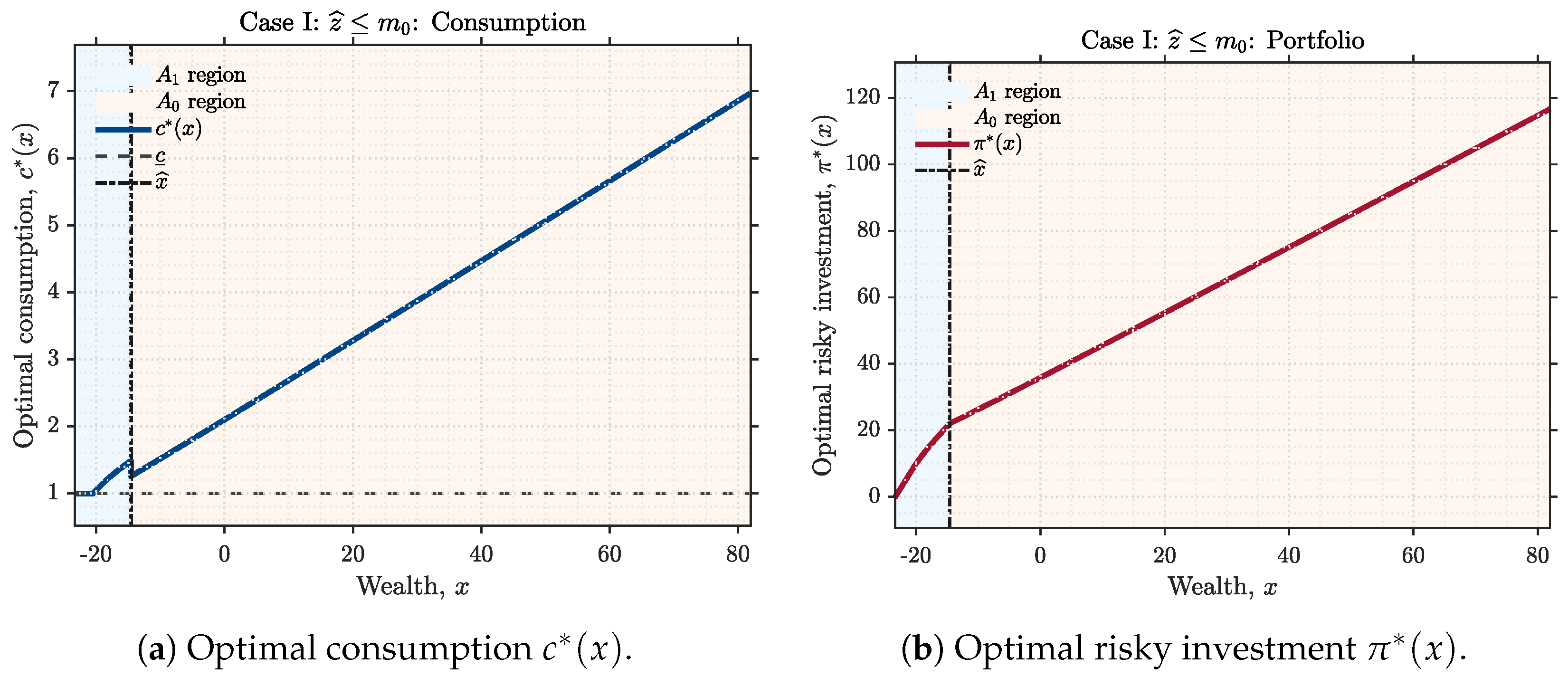
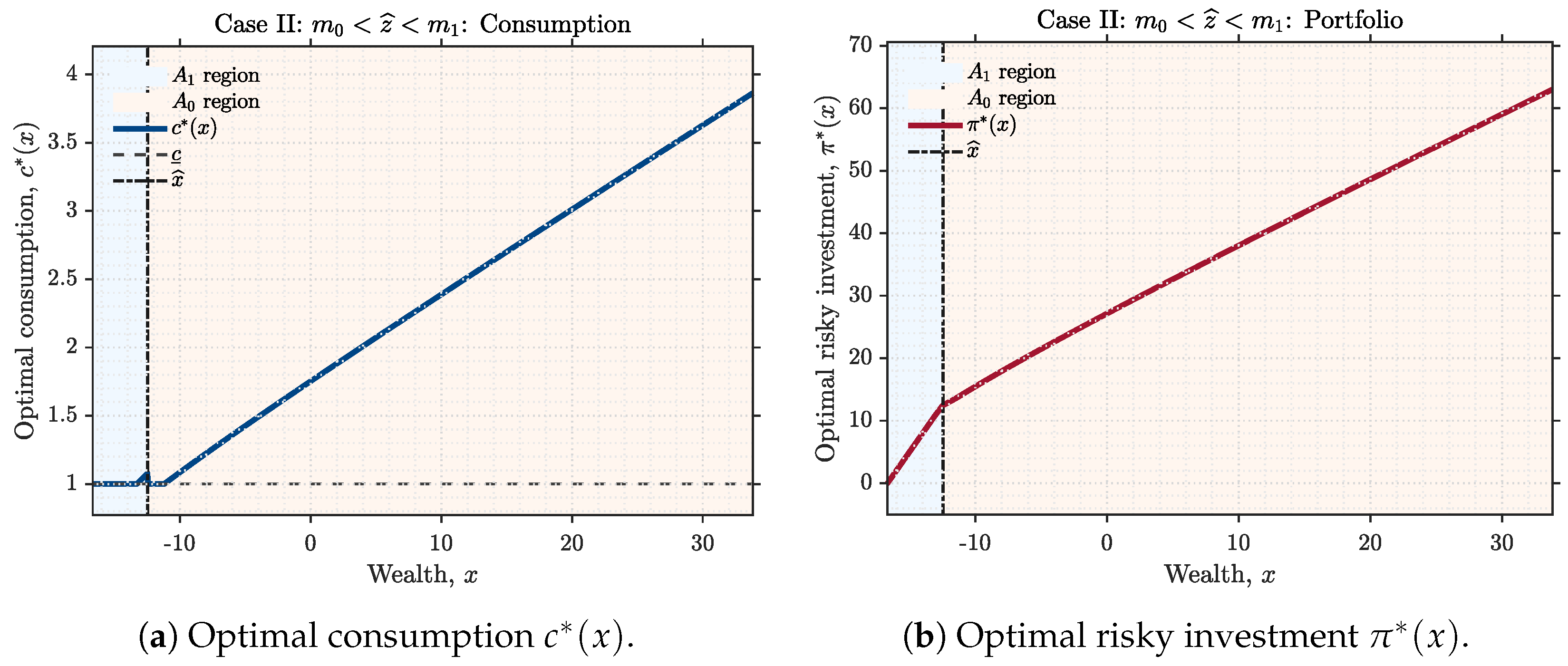
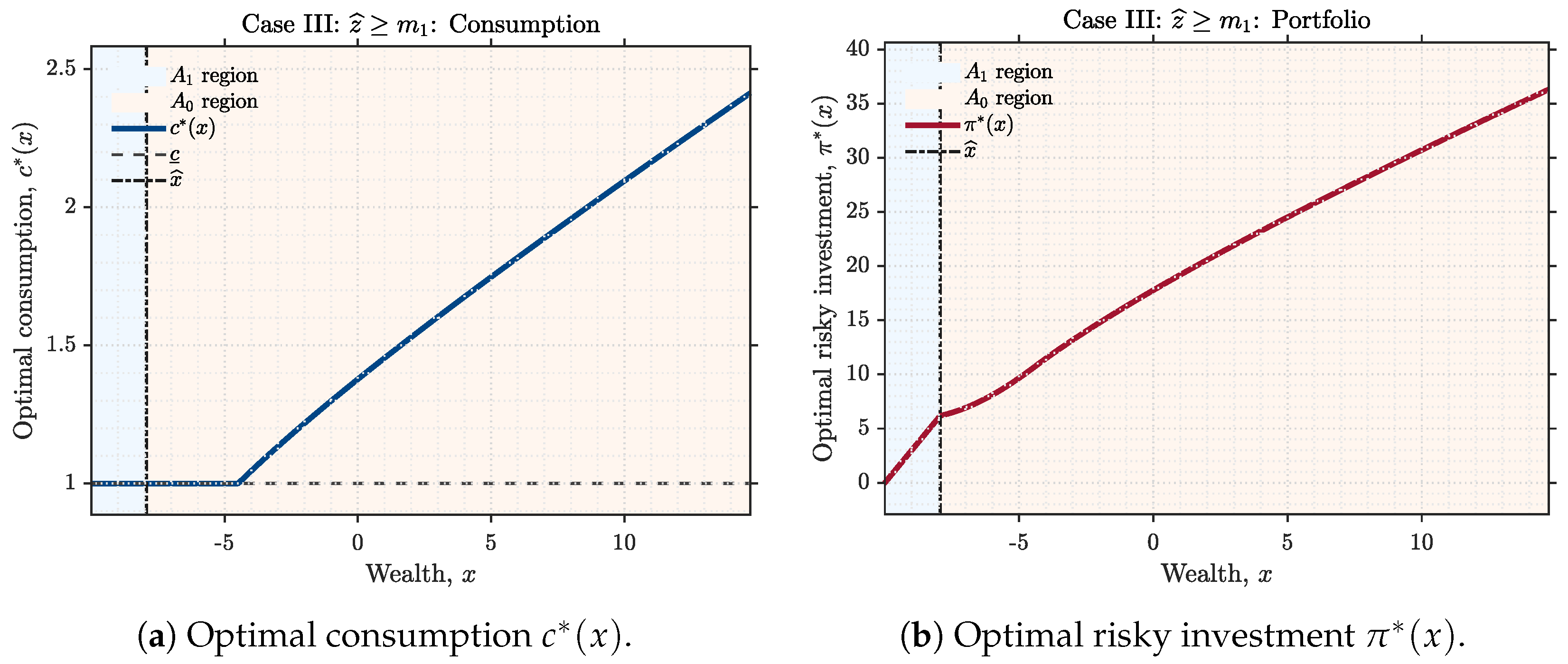
This section uses the zoomed policy plots to illustrate how the subsistence requirement changes the observable shape of the optimal consumption and portfolio rules. Figure 1, Figure 2 and Figure 3 focus on a narrow wealth range around the switching threshold $\widehat{x}$, so that the differences across the three cases become visually transparent.

Table 2. Parameter values and implied quantities for Figure 1, Figure 2 and Figure 3.

	Case I	Case II	Case III
Figure	Figure 1	Figure 2	Figure 3
Regime condition	$\delta \ge {\delta }_u$	${\delta }_b<\delta <{\delta }_u$	$\delta \le {\delta }_b$
r	0.03	0.03	0.03
$\mu$	0.09	0.09	0.09
$\sigma$	0.20	0.20	0.20
$\rho$	0.06	0.06	0.06
$\gamma$	2.00	2.00	2.00
$\alpha$	0.50	0.50	0.50
$Y_0$	1.00	1.00	1.00
$Y_1$	1.70	1.50	1.30
$\delta =Y_1-Y_0$	0.70	0.50	0.30
$L_0$	1.00	1.00	1.00
$L_1$	0.60	0.60	0.60
$\underline{c}$	1.00	1.00	1.00
${\gamma }_1$	1.50	1.50	1.50
$\theta$	0.30	0.30	0.30
$K_1$	0.06	0.06	0.06
${\delta }_b$	0.451	0.451	0.451
${\delta }_u$	0.557	0.557	0.557
$m_0$	1.000	1.000	1.000
$m_1$	1.291	1.291	1.291
$\widehat{z}$	0.710	1.154	1.940
$\widehat{x}$	$-14.559$	$-12.456$	$-7.939$
$\underline{x}$	$-23.333$	$-16.667$	$-10.000$

and

Table 3. Numerical setup for the comparative-statics exercise in Figure 4.

Item	Value
Varied parameter	$\delta =Y_1-Y_0$
Definition of $Y_1$ on the grid	$Y_1=Y_0+\delta$
Fixed primitive parameters	$(r,\mu ,\sigma ,\rho ,\gamma ,\alpha ,Y_0,L_0,L_1,\underline{c})=(0.03,0.09,0.20,0.06,2.00,0.50,1.00,1.00,0.60,1.00)$
Implied common parameters	$({\gamma }_1,\theta ,K_1)=(1.50,0.30,0.06)$
Grid for $\delta$	301 equally spaced points on $[0.180,0.752]$
Critical gap ${\delta }_b$	0.451
Critical gap ${\delta }_u$	0.557
Case III on plotted grid	$\delta \le {\delta }_b$; approximately $[0.180,0.449]$ on the grid
Case II on plotted grid	${\delta }_b<\delta <{\delta }_u$; approximately $[0.451,0.556]$ on the grid
Case I on plotted grid	$\delta \ge {\delta }_u$; approximately $[0.558,0.752]$ on the grid
Plotted quantities	$\widehat{x}\left(\delta \right)$ and the lengths of $\{x:c^{*}\left(x\right)=\underline{c}\}$, decomposed into the $A_1$ and $A_0$ floor segments

report the primitive and implied parameter values used to generate the numerical figures. The first table makes each of the three baseline figure pairs reproducible, while the second table records the grid and fixed parameters used in the comparative-statics exercise. In Figure 4, only the income gap $\delta =Y_1-Y_0$ varies; all other primitive parameters are held fixed.

The entries are rounded for presentation; the numerical figures were generated using the corresponding unrounded values.

In all panels, the shaded blue region corresponds to the high-income job $A_1$, while the shaded light-orange region corresponds to the high-leisure job $A_0$. The vertical dash-dotted line marks the switching boundary $\widehat{x}$. In the consumption panels, the horizontal dashed line indicates the subsistence floor $\underline{c}$.

The figures reveal three robust qualitative implications. First, in every case the agent chooses the high-income job $A_1$ when wealth is low and switches to the high-leisure job $A_0$ only after wealth exceeds the threshold $\widehat{x}$. Second, the stronger is the role of the subsistence floor at the switching point, the flatter is the consumption function near $\widehat{x}$. Third, the optimal risky investment is increasing in wealth in all three cases, but its level near the switching point is highest in Case I and lowest in Case III. Thus the subsistence constraint affects not only labor supply but also the shape of the consumption and portfolio rules around the switching region.

The three cases together deliver a clean comparative-statics message. Moving from Case I to Case III, the switching point is pushed deeper into the financially constrained region, so the neighborhood of $\widehat{x}$ becomes increasingly dominated by the subsistence floor. As a result, the optimal consumption rule becomes progressively flatter near the switching point:

• in Case I, the floor is already slack at the switching point;
• in Case II, the floor binds only after the switch to $A_0$;
• in Case III, the floor binds already before the switch and continues to bind afterward.

Hence the shape of the consumption curve around $\widehat{x}$ provides a direct visual diagnosis of which regime the economy is in.

The portfolio figures provide a complementary implication. In all three cases, the risky position is increasing in wealth, which is consistent with the standard intuition that wealthier agents can bear more financial risk. However, the level of ${\pi }^{*}\left(x\right)$ near the switching boundary is markedly regime-dependent. Case I exhibits the largest risky position near $\widehat{x}$, whereas Case III exhibits the smallest. Thus a stronger subsistence motive suppresses financial risk-taking around the job-switching region.

Taken together, Figure 1, Figure 2 and Figure 3 show that the subsistence constraint affects the model through two distinct channels. The first channel is a labor-supply channel: at low wealth the agent remains in the high-income job $A_1$ for longer. The second channel is a policy-distortion channel: the floor flattens consumption and lowers risky investment around the switching boundary. These effects are weakest in Case I, stronger in Case II, and strongest in Case III.

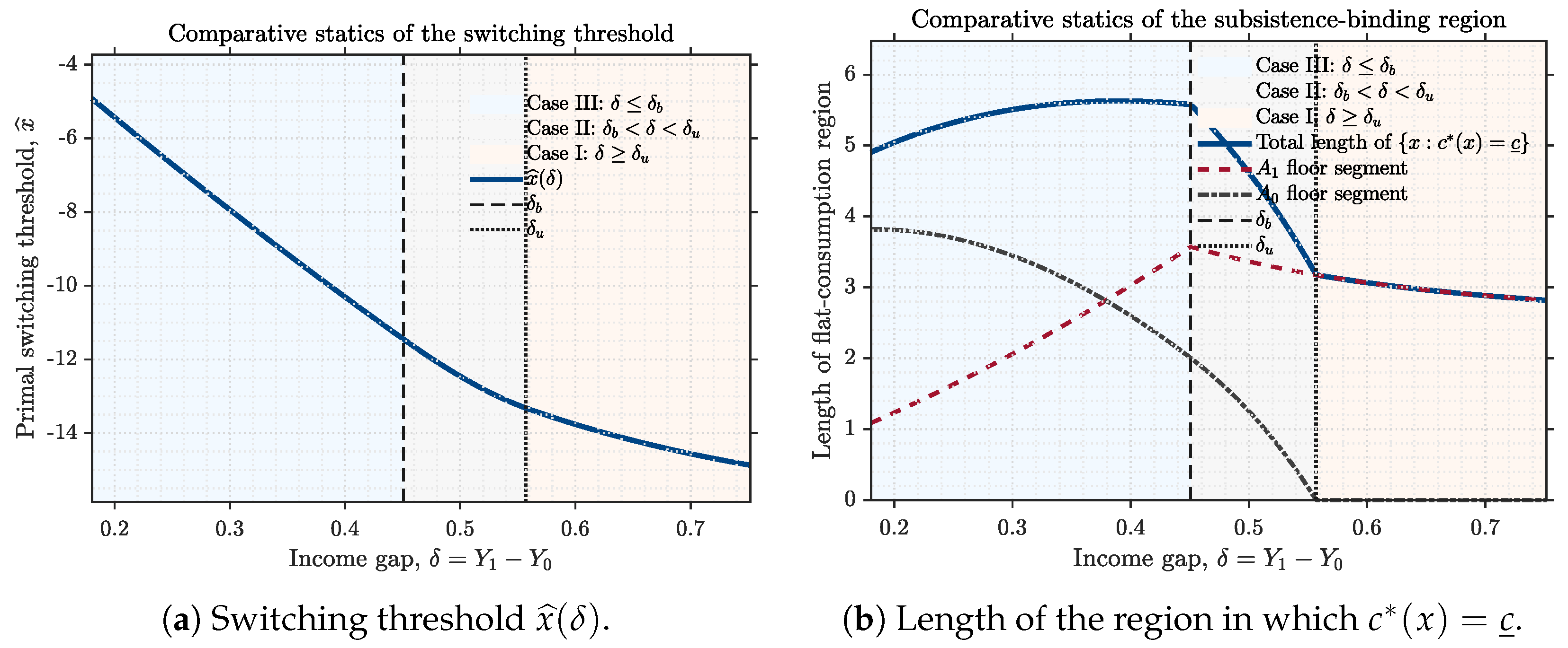
Figure 4 complements the three illustrative cases by varying the income gap $\delta =Y_1-Y_0$ continuously while holding the other parameters fixed. Panel (a) shows that the primal switching threshold $\widehat{x}\left(\delta \right)$ is decreasing in the income gap. As the high-income job becomes more attractive relative to the high-leisure job, the relevant switching boundary moves monotonically across the three analytical regimes. The two critical gaps ${\delta }_b$ and ${\delta }_u$ are visible as regime-separating points rather than as numerical artifacts: the curve remains continuous, but its slope changes when the dual switching point moves from the binding–binding region to the mixed binding–slack region and then to the slack–slack region.

Panel (b) decomposes the flat-consumption region $\{x:c^{*}\left(x\right)=\underline{c}\}$ into the part generated while the agent works in the high-income job $A_1$ and the part generated while the agent works in the high-leisure job $A_0$. In Case III, the floor binds at the switching point under both jobs, so the flat region contains both an $A_1$ segment and an $A_0$ segment. As $\delta$ increases toward ${\delta }_u$, the $A_0$ floor segment shrinks and eventually disappears. Once $\delta \ge {\delta }_u$, the floor is already slack at the switching threshold, so the remaining flat region is entirely associated with low-wealth states in the $A_1$ region. This comparative-static exercise confirms that the three regimes are not merely isolated examples; they describe systematic changes in the location of the switching threshold and in the size and composition of the subsistence-binding consumption region.

11. Conclusions

This paper provides a subsistence-constrained extension of the reversible job-choice model of Shim and Shin [11] in the case $\gamma >1$. The consumption floor changes the dual consumption demand from $a_i{z}^{-1/{\gamma }_1}$ to $max\{\underline{c},a_i{z}^{-1/{\gamma }_1}\}$. As a result, the job-selection payoff becomes the upper envelope of two piecewise dual rewards. We prove that the subsistence-adjusted switching function has a unique positive zero. We further characterize the location of this zero using two critical income gaps, ${\delta }_b$ and ${\delta }_u$. Therefore the optimal job policy remains a one-threshold rule in wealth, but the boundary is shifted by the subsistence constraint. Near the solvency boundary, the agent consumes at the subsistence level and necessarily chooses the high-income job. The dual value function is available in closed form in all regimes through explicit coefficient-jump formulas.

The economic implication is that subsistence needs create a precautionary labor-supply force. When wealth is close to the solvency boundary, consumption cannot be reduced below basic needs, so the high-income job becomes the only margin through which the agent can relax the intertemporal budget pressure. This mechanism provides a simple theoretical explanation for why low-wealth households may remain in less desirable but higher-paying jobs even when a higher-leisure job is available. The model also implies that subsistence requirements affect financial decisions: by flattening consumption near the floor, they alter the marginal value of wealth and therefore the optimal risky position around the switching threshold.

From a policy perspective, the results suggest that labor-market flexibility and household financial risk-taking cannot be fully understood without accounting for non-discretionary consumption commitments. Policies that reduce basic expenditure burdens, such as housing-cost relief, medical-expense insurance, or income support targeted at low-wealth households, may affect not only consumption smoothing but also occupational choice and portfolio behavior. In the model, such policies operate by shifting the effective subsistence level $\underline{c}$ and hence the critical income gaps ${\delta }_b$ and ${\delta }_u$ that determine the relevant switching regime.

The analysis has several limitations. We abstract from switching costs, unemployment risk, finite horizons, borrowing constraints beyond the natural solvency boundary, stochastic labor income, and endogenous leisure choices within each job. We also focus on the case $\gamma >1$, which delivers a clean single-crossing structure and closed-form solution. These simplifications are deliberate: they allow us to isolate the subsistence-consumption channel in the benchmark reversible job-choice problem. Future research could combine the present subsistence mechanism with costly switching, unemployment risk, finite-horizon retirement decisions, or incomplete markets. In a spanned stochastic-income extension, one could replace the constant income term $Y_i/r$ by the state-price value of job-specific income; in an unspanned stochastic-income extension, the dual problem would become an incomplete-market problem and the closed-form threshold would generally be lost. Job-specific consumption floors would be a more direct deterministic extension and would modify the break points $m_i$ without changing the basic Fenchel-transform logic. Another natural extension is to study whether the single-threshold structure survives under more general preferences or under parameter regions in which $\gamma \le 1$.