The Variation Iteration Method Combined with the Natural Generalized Laplace Transform for Solving Fractional Burgers Equations

Abstract

In this work, we solve fractional Burgers equations by using the new natural generalized Laplace transform (NGLT) and double natural generalized Laplace transform (DNGLT) methods with the variation iteration method. First, we present the basic definitions of natural transforms, the generalized Laplace transform, and Caputo fractional derivatives, which provide the theoretical basis of this work. This work is mainly concerned with the natural generalized Laplace variational iteration method (NGLTVIM), which is a new approach for the solution of conventional problems. The stability and convergence of the proposed method are discussed in detail to prove its reliability and effectiveness. The efficiency of the method for finding solutions to one-dimensional and singular fractional coupled Burgers equations is illustrated by several numerical examples. The results demonstrate that NGLTVIM can be successfully applied to solving various problems of mathematical physics.

1. Introduction

The fractional Burgers equation is an important mathematical model used in fluid dynamics and diffusion systems. This equation includes the Caputo fractional derivatives in the classical Burgers equation, which describes the evolution of viscous fluid flows. These derivatives provide tools for modeling anomalous diffusion and nonlocal effects, which are common in various physical applications such as turbulence and viscoelastic materials.The natural transform and the Adomian decomposition method are two effective approaches that have been used to create the Natural Transform Decomposition Method. NTDM is employed to solve various physical phenomena that are described by PDEs and fractional PDEs. The analytical solution of a couple of systems of nonlinear PDEs is recommended in [1], the solution to nonlinear ODEs has been successfully provided in [2], fractional turbulent flow of a polytropic gas model was demonstrated in [3], and fractional Fokker–Planck and Schrodinger equations were used in [4]. In [5], the analytical solutions of fourth-order parabolic partial differential equations with time-fractional derivatives and variable coefficients are presented using the modified Laplace variational iteration approach and the homotopy perturbation method. Many researchers in the literature have used the variation iteration method to obtain solutions of partial differential equations and fractional differential equations. For example, the method was applied to solve multi-dimensional fractional integral–differential equations, as discussed in [6]. The authors in [7] studied the solution of nonlinear integral–differential equations by using two different methods: the Laplace Adomian decomposition method and the series solution method. In [8], the authors proposed a new generalized method to solve fractional convection-diffusion equations based on the famous variational iteration method (VIM) modified by an additional parameter. The analytical Differential Transform Method (DTM) and Physics-informed Neural Networks (PINNs) are used to solve Volterra and Fredholm integral equations [9]. The Group Teaching Optimization Algorithm (GTOA) method is used to solve the inverse problem for a model consisting of a fractional differential equation with the Caputo derivative and the Riemann–Liouville derivative in the case of space [10]. The authors in [11] examined solutions of the Fokker–Planck equation and fractional diffusion equations using the Laplace variational iteration method. In [4], the Natural Transform Decomposition Method was employed to obtain solutions of fractional-order partial differential equations with proportional delay. The authors in [12] employed a new Laplace variational iteration method to obtain solutions for (2+1)-D and (3+1)-D Burgers equations. Approximate solutions to time-fractional system partial differential equations using the natural generalized Laplace transform are presented in [13]. The natural transform iterative method (NTIM) was applied to study solutions of fractional differential equations (FDEs), as explained in [14]. Solutions of partial differential equations via the Natural Transform Decomposition Method are presented in [4,15,16,17].

This work aims to investigate the applicability of combining the variation iteration method (VIM) and the natural generalized Laplace transform (NGLT) to obtain solutions of the fractional Burgers equation. This combined approach is referred to as the natural generalized Laplace variational iteration method (NGLVIM).

Let us recall the definitions of the natural transform (NT) and the generalized Laplace transform (GLT), respectively.

Definition 1. 

Over the set of functions

$$A=\left\{\begin{array}{c}f\left(x\right):\exists M,{\tau }_1,{\tau }_2>0,\mathit{such}\mathit{that}\\ \left|f\left(x\right)\right|<M{e}^{{\displaystyle \frac{\left|x\right|}{{\tau }_j}}},\mathrm{if}\delta \in {(-1)}^j\times [0,\infty ),j=1,2,\end{array}\right\},$$

the natural transform (NT) is defined by

$${\mathrm{N}}_x^{+}\left[f\left(x\right)\right]=R\left(p;u\right)={\displaystyle \frac{1}{u}}{\int }_0^{\infty }{e}^{-{\displaystyle \frac{p}{u}}x}f\left(x\right)dx,\mathrm{Re}\left(p\right),\mathrm{Re}\left(u\right)>0,$$

(1)

where u and p are complex variables of the transform in Equation (5). For more details, see [4].

Definition 2 

([18]). Let $f\left(\delta \right)$ be an integrable function for all $\delta \ge 0$. The generalized Laplace transform $G_{\alpha }$ of $f\left(\delta \right)$ is defined by

$$F\left(s\right)=G_{\alpha }\left(f\right)=s^{\alpha }{\int }_0^{\infty }f\left(\delta \right)e^{-{\displaystyle \frac{\delta }{s}}}d\delta ,$$

(2)

for $s\in \mathbb{C}$ and $\alpha \in \mathbb{Z}$.

Definition 3 

([19]). The Liouville–Caputo partial derivative of a function $\varphi (x,\delta )$, where $(x,\delta )\in {\mathbb{R}}^{+}\times {\mathbb{R}}^{+}$, is given by

$${}^{C}D_{\delta }^{\beta }\varphi ={\displaystyle \frac{{\partial }^{\beta }\varphi \left(x,\delta \right)}{\partial {\delta }^{\beta }}}=\left\{\begin{array}{cc}{\displaystyle \frac{{\partial }^n\varphi \left(x,\delta \right)}{\partial {\delta }^n}},\hfill & \beta =n,\hfill \\ I^{n-\beta }\left[{\displaystyle \frac{{\partial }^n\varphi \left(x,\delta \right)}{\partial {\delta }^n}}\right],\hfill & n-1<\beta <n,n\in \mathbb{N},\hfill \end{array}\right.$$

Theorem 1 

(Banach’s fixed-point theorem [20]). Let $(\Omega ,d)$ be a metric space, where $\Omega \ne \varnothing$. Suppose that $\Omega$ is complete and let $\Lambda :\Omega \to \Omega$ be a contraction on $\Omega$. Then, $\Lambda$ has a unique fixed point.

Theorem 2 

([21]). Let $(\Omega ,\parallel ·\parallel )$ be a Banach space and let $\Lambda :\Omega \to \Omega$ be a self-map satisfying

$$\parallel {\Lambda }_x-{\Lambda }_y\parallel \le K\parallel x-{\Lambda }_x\parallel +\eta \parallel x-y\parallel ,\forall x,y\in \Omega ,K\ge 0,0<\eta <1,$$

so Λ is Picard Λ-stable.

2. Properties of Natural Generalized Laplace Transform

In this section, we introduce the basic concepts and properties of the natural generalized Laplace transform (NGLT). The NGLT is defined as follows:

$$\begin{array}{ccc}\hfill {\mathrm{N}}_x^{+}{G}_{\delta }\left[f\left(x,\delta \right)\right]& =& F\left(p;u,s\right)={\displaystyle \frac{s^{\alpha }}{u}}{\int }_0^{\infty }{\int }_0^{\infty }{e}^{-{\displaystyle \frac{p}{u}}x-{\displaystyle \frac{1}{s}}\delta }f(x,\delta )d\delta dx,\hfill \\ & & \mathrm{Re}\left(s\right),\mathrm{Re}\left(p\right)>0,\mathrm{Re}\left(u\right)>0,\hfill \end{array}$$

(3)

For more details, see [22] and

$$\begin{array}{ccc}\hfill {\mathrm{N}}_{x,y}^{+}{G}_{\delta }\left[f\left(x,y,\delta \right)\right]& =& F\left(p;u,q,v;s\right)={\displaystyle \frac{s^{\alpha }}{uv}}{\int }_0^{\infty }{\int }_0^{\infty }{\int }_0^{\infty }{e}^{-{\displaystyle \frac{p}{u}}x-{\displaystyle \frac{q}{v}}y-{\displaystyle \frac{1}{s}}\delta }f(x,y,\delta )d\delta dydx,\hfill \\ & & \mathrm{Re}\left(s\right),\mathrm{Re}\left(p\right)>0,\mathrm{Re}\left(u\right)>0,\mathrm{Re}\left(v\right)>0.\hfill \end{array}$$

For additional details, see [22]. Here, ${\mathrm{N}}_x^{+}{G}_{\delta }$ denotes the NGLT, while ${\mathrm{N}}_{x,y}^{+}{G}_{\delta }$ denotes the double natural generalized Laplace transform (DNGLT). The inverse NGLT and DNGLT are given by

$${\mathrm{N}}_{p;u}^{-1}{G}_s^{-1}\left(F\left(p;u,s\right)\right)=f\left(x,\delta \right)={\displaystyle \frac{1}{{\left(2\pi i\right)}^2}}{\int }_{\lambda -i\infty }^{\lambda +i\infty }{\int }_{\sigma -i\infty }^{\sigma +i\infty }{e}^{{\displaystyle \frac{p}{u}}x+{\displaystyle \frac{1}{s}}\delta }F\left(p;u,s\right)dsdp,$$

and

$$\begin{array}{ccc}\hfill {\mathrm{N}}_2^{-1}{G}_s^{-1}\left(F\left(p,u;q,v;s\right)\right)& =& f\left(x,y,\delta \right)\hfill \\ & =& {\displaystyle \frac{1}{{\left(2\pi i\right)}^3}}{\int }_{\lambda -i\infty }^{\lambda +i\infty }{\int }_{\sigma -i\infty }^{\sigma +i\infty }{\int }_{\vartheta -i\infty }^{\vartheta +i\infty }{e}^{{\displaystyle \frac{p}{u}}x+{\displaystyle \frac{1}{s}}\delta }F\left(p,u;q,v;s\right)dsdqdp.\hfill \end{array}$$

Remark 1. 

Based on the definition of the NGLT, we derive the following transforms:

1. 

Setting $\alpha =-1$, $p=1$, and $s=v$, we obtain the double Sumudu transform:

$${\mathrm{S}}_x{S}_{\delta }\left[f\left(x,\delta \right)\right]=F\left(u,v\right)={\displaystyle \frac{1}{uv}}{\int }_0^{\infty }{\int }_0^{\infty }{e}^{-{\displaystyle \frac{1}{u}}x-{\displaystyle \frac{1}{v}}\delta }f(x,\delta )d\delta dx.$$

2. 

Setting $\alpha =0$, $u=1$, and $s={\displaystyle \frac{1}{s}}$, we obtain the double Laplace transform:

$$L_x{L}_{\delta }\left[f\left(x,\delta \right)\right]=F\left(p,s\right)={\int }_0^{\infty }{\int }_0^{\infty }{e}^{-px-s\delta }f(x,\delta )d\delta dx.$$

3. 

Setting $\alpha =0$, $u=1$, and $s=\varphi$, we obtain the Laplace–Yang transform:

$$L_{x}Y\left[f\left(x,\delta \right)\right]=F\left(p,\varphi \right)={\int }_0^{\infty }{\int }_0^{\infty }{e}^{-px-{\displaystyle \frac{1}{\varphi }}\delta }f(x,\delta )d\delta dx.$$

The following examples are useful in this work.

• The NGLT of the function $f(x,\delta )=e^{ax+b\delta }$ is given by

$$F\left(p;u,s\right)={\mathrm{N}}_x^{+}{G}_{\delta }\left[e^{ax+b\delta }\right]={\displaystyle \frac{1}{\left(p-au\right)}}{\displaystyle \frac{s^{\alpha +1}}{1-bs}}.$$

The NGLT of $f(x,\delta )={\left(x\delta \right)}^n$ is given by

$${\mathrm{N}}_x^{+}{G}_{\delta }\left[{\left(x\delta \right)}^n\right]={\displaystyle \frac{{\left(n!\right)}^2{u}^n{s}^{n+\alpha +1}}{p^{n+1}}},$$

where n is a positive integer.

If $a>-1$ and $b>-1$ are real numbers, then

$${\mathrm{N}}_x^{+}{G}_{\delta }\left[x^a{\delta }^b\right]={\displaystyle \frac{u^a\Gamma \left(a+1\right)\Gamma \left(b+1\right)s^{\alpha +b+1}}{p^{a+1}}}.$$

This result follows from the definition of the NGLT,

$$\begin{array}{ccc}\hfill {\mathrm{N}}_x^{+}{G}_{\delta }\left[x^a{\delta }^b\right]& =& {\displaystyle \frac{s^{\alpha }}{u}}{\int }_0^{\infty }{\int }_0^{\infty }{e}^{-{\displaystyle \frac{p}{u}}x-{\displaystyle \frac{s}{v}}\delta }{x}^a{\delta }^{b}d\delta dx\hfill \\ & =& {\displaystyle \frac{1}{u}}{\int }_0^{\infty }{e}^{-{\displaystyle \frac{p}{u}}x}{x}^a\left(s^{\alpha }{\int }_0^{\infty }{e}^{-{\displaystyle \frac{1}{s}}\delta }{\delta }^{b}d\delta \right)dx.\hfill \end{array}$$

By applying the substitutions ${\displaystyle \frac{p}{u}}x=r$ and ${\displaystyle \frac{1}{s}}\delta =q$, we obtain

$$\begin{array}{ccc}\hfill {\mathrm{N}}_x^{+}{G}_{\delta }\left[x^a{\delta }^b\right]& =& {\displaystyle \frac{1}{u}}{\int }_0^{\infty }{\left({\displaystyle \frac{u}{p}}r\right)}^a{e}^{-r}{\displaystyle \frac{u}{p}}dr{s}^{\alpha }{\int }_0^{\infty }{\left(sq\right)}^b{e}^{-q}sdq\hfill \\ & =& {\displaystyle \frac{u^a}{p^{a+1}}}{s}^{\alpha +b+1}{\int }_0^{\infty }{\int }_0^{\infty }{r}^a{q}^b{e}^{-r}{e}^{-q}drdq\hfill \\ & =& {\displaystyle \frac{u^a\Gamma \left(a+1\right)\Gamma \left(b+1\right)s^{\alpha +b+1}}{p^{a+1}}},\hfill \end{array}$$

where the gamma functions of a and b are defined by the uniformly convergent integral as follows.

$$\Gamma \left(a\right)\Gamma \left(b\right)={\int }_0^{\infty }{e}^{-r}{r}^{a-1}dr{\int }_0^{\infty }{e}^{-q}{q}^{b-1}dq,a>0,b>0.$$

Definition 4. 

Let $\Lambda :\Omega \to \Omega$ be a mapping. A point $x\in \Omega$ is called a fixed point of Λ if 

$${\Lambda }_x=x.$$

Definition 5 

([23]). Let $(\Omega ,d)$ be a metric space. A mapping $\Lambda :\Omega \to \Omega$ is called a contraction if there exists a constant $0\le K<1$ such that for all $x,y\in \Omega$,

$$d\left({\Lambda }_x,{\Lambda }_y\right)\le Kd\left(x,y\right).$$

Theorem 3. 

The DNGLT of the partial derivative ${}^{C}D_{\delta }^{\beta }\varphi$ is given by

$${\mathrm{N}}_2^{+}{G}_{\alpha }\left[{}^{C}D_{\delta }^{\beta }\varphi \right]={\displaystyle \frac{\Phi }{s^{\beta }}}-{\displaystyle \sum _{k=1}^n}{s}^{\alpha +k-\beta }{\displaystyle \frac{{\partial }^{k-1}\varphi \left(p,u;q,v,0\right)}{\partial {\delta }^{k-1}}},$$

where $\Phi =\Phi (p,u;q,v;s)$ is the DNGLT of $\varphi (x,y,\delta )$.

Proof. 

By using the definition of Caputo fractional derivative

$${}^{C}D_{\delta }^{\beta }\varphi ={\displaystyle \frac{1}{\Gamma \left(n-\beta \right)}}{\displaystyle \underset{0}{\overset{\delta }{\int }}}{\left(\delta -\eta \right)}^{n-\beta -1}{\displaystyle \frac{{\partial }^n\varphi \left(x,y,\eta \right)}{\partial {\eta }^n}}d\eta ={}_0{}^{c}I^{n-\beta }{\displaystyle \frac{{\partial }^n\varphi }{\partial t^n}},$$

applying DNGLT

$$\begin{array}{ccc}\hfill {\mathbf{N}}_2^{+}{G}_{\alpha }\left[{}^{C}D_{\delta }^{\beta }\varphi \right]& =& {\mathbf{N}}_2^{+}{G}_{\alpha }\left[{}_0{}^{c}I^{n-\beta }{\displaystyle \frac{{\partial }^n\varphi }{\partial t^n}}\right]\hfill \\ & =& {\displaystyle \frac{1}{\Gamma \left(n-\beta \right)}}{\mathbf{N}}_2^{+}{G}_{\alpha }\left[{\displaystyle \underset{0}{\overset{\delta }{\int }}}{\left(\delta -\eta \right)}^{n-\beta -1}{\displaystyle \frac{{\partial }^n\varphi \left(x,y,\eta \right)}{\partial {\eta }^n}}d\eta \right],\hfill \end{array}$$

one may express the integral within the brackets via the convolution operator as follows:

$${\mathbf{N}}_2^{+}{G}_{\alpha }\left[{}^{C}D_{\delta }^{\beta }\varphi \right]={\displaystyle \frac{1}{\Gamma \left(n-\beta \right)}}{\mathbf{N}}_2^{+}{G}_{\alpha }\left[{\delta }^{n-\beta -1}***{\displaystyle \frac{{\partial }^n\varphi \left(x,y,\delta \right)}{\partial {\delta }^n}}\right],$$

Using the DNGLT for convolution, the previous equation is

$$\begin{array}{ccc}\hfill {\mathbf{N}}_2^{+}{G}_{\alpha }\left[{}^{C}D_{\delta }^{\beta }\varphi \right]& =& {\displaystyle \frac{uv}{\Gamma \left(n-\beta \right)s^{\alpha }}}{\mathbf{N}}_2^{+}{G}_{\alpha }\left[{\delta }^{n-\beta -1}\right]{\mathbf{N}}_2^{+}{G}_{\alpha }\left[{\displaystyle \frac{{\partial }^n\varphi }{\partial {\delta }^n}}\right]\hfill \\ & =& {\displaystyle \frac{uv\Gamma \left(n-\beta \right)s^{n-\beta +\alpha }}{\Gamma \left(n-\beta \right)s^{\alpha }uv}}\left[{\displaystyle \frac{\Phi }{s^n}}-s^{\alpha }{\displaystyle \sum _{k=1}^n}{\displaystyle \frac{1}{s^{n-k}}}{\displaystyle \frac{{\partial }^{k-1}\varphi \left(p,u;q,v,0\right)}{\partial {\mathsf{\delta }}^{k-1}}}\right]\hfill \\ & =& {\displaystyle \frac{\Phi }{s^{\beta }}}-s^{n-\beta +\alpha }{\displaystyle \sum _{k=1}^n}{\displaystyle \frac{1}{s^{n-k}}}{\displaystyle \frac{{\partial }^{k-1}\varphi \left(p,u;q,v,0\right)}{\partial {\mathsf{\delta }}^{k-1}}}\hfill \\ \hfill {\mathbf{N}}_2^{+}{G}_{\alpha }\left[{}^{C}D_{\delta }^{\beta }\varphi \right]& =& {\displaystyle \frac{\Phi }{s^{\beta }}}-{\displaystyle \sum _{k=1}^n}{s}^{k-\beta +\alpha }{\displaystyle \frac{{\partial }^{k-1}\varphi \left(p,u;q,v,0\right)}{\partial {\mathsf{\delta }}^{k-1}}}.\hfill \end{array}$$

□

Theorem 4. 

The DNGLT of $x{D}_{\delta }^{\beta }\varphi$ and $y{D}_{\delta }^{\beta }\varphi$ are given by

$$\begin{array}{ccc}\hfill {\mathrm{N}}_2^{+}{G}_{\alpha }\left[x{D}_{\delta }^{\beta }\varphi \right]& =& {\displaystyle \frac{u}{p{s}^{\beta }}}{\displaystyle \frac{d}{du}}\left(u\Phi (p;u,q;v,s)\right)\hfill \\ & & -{\displaystyle \frac{u{s}^{\alpha -\beta +1}}{p}}{\displaystyle \frac{d}{du}}\left(u\Phi (p;u,q;v,0)\right),\hfill \end{array}$$

(4)

and

$$\begin{array}{ccc}\hfill {\mathrm{N}}_2^{+}{G}_{\alpha }\left[y{D}_{\delta }^{\beta }\varphi \right]& =& {\displaystyle \frac{v}{q{s}^{\beta }}}{\displaystyle \frac{d}{dv}}\left(v\Phi (p;u,q;v,s)\right)\hfill \\ & & -{\displaystyle \frac{v{s}^{\alpha -\beta +1}}{q}}{\displaystyle \frac{d}{dv}}\left(v\Phi (p;u,q;v,0)\right),\hfill \end{array}$$

(5)

where

$$\Phi \left(p;u,q;v,s\right)={\mathbf{N}}_2^{+}{G}_{\alpha }\left[\varphi \left(x,y,t\right)\right].$$

Proof. 

From the definition of the DNGLT, we have

$${\mathrm{N}}_2^{+}{G}_{\alpha }\left[D_{\delta }^{\beta }\varphi \right]={\displaystyle \frac{s^{\alpha }}{uv}}{\int }_0^{\infty }{\int }_0^{\infty }{\int }_0^{\infty }{e}^{-({\displaystyle \frac{p}{u}}x+{\displaystyle \frac{q}{v}}y+{\displaystyle \frac{\delta }{s}})}{D}_{\delta }^{\beta }\varphi dxdyd\delta .$$

(6)

Differentiating with respect to u for each part of Equation (6), we get

$$\begin{array}{cc}\hfill {\displaystyle \frac{d}{du}}\left({\mathrm{N}}_2^{+}{G}_{\alpha }\left[D_{\delta }^{\beta }\varphi \right]\right)=& {\displaystyle \frac{s^{\alpha }}{v}}{\displaystyle \underset{0}{\overset{\infty }{\int }}}{\displaystyle \underset{0}{\overset{\infty }{\int }}}{e}^{-{\displaystyle \frac{q}{v}}y-{\displaystyle \frac{\delta }{s}}}\left[{\displaystyle \underset{0}{\overset{\infty }{\int }}}{\displaystyle \frac{d}{du}}\left({\displaystyle \frac{1}{u}}{e}^{-{\displaystyle \frac{p}{u}}x}\right)dx\right]D_{\delta }^{\beta }\varphi dyd\delta \hfill \\ \hfill & ={\displaystyle \frac{s^{\alpha }}{v}}{\displaystyle \underset{0}{\overset{\infty }{\int }}}{\displaystyle \underset{0}{\overset{\infty }{\int }}}{e}^{-{\displaystyle \frac{q}{v}}y-{\displaystyle \frac{\delta }{s}}}\left[{\displaystyle \underset{0}{\overset{\infty }{\int }}}\left(-{\displaystyle \frac{1}{u^2}}+{\displaystyle \frac{p}{u^3}}x\right)e^{-{\displaystyle \frac{p}{u}}x}dx\right]D_{\delta }^{\beta }\varphi dyd\delta \hfill \\ \hfill & =-{\displaystyle \frac{s^{\alpha }}{u^{2}v}}{\displaystyle \underset{0}{\overset{\infty }{\int }}}{\displaystyle \underset{0}{\overset{\infty }{\int }}}{\displaystyle \underset{0}{\overset{\infty }{\int }}}{e}^{-({\displaystyle \frac{p}{u}}x+{\displaystyle \frac{q}{v}}y+{\displaystyle \frac{\delta }{s}})}{D}_{\delta }^{\beta }\varphi dxdyd\delta \hfill \\ \hfill & +{\displaystyle \frac{s^{\alpha }p}{u^{3}v}}{\displaystyle \underset{0}{\overset{\infty }{\int }}}{\displaystyle \underset{0}{\overset{\infty }{\int }}}{\displaystyle \underset{0}{\overset{\infty }{\int }}}{e}^{-({\displaystyle \frac{p}{u}}x+{\displaystyle \frac{q}{v}}y+{\displaystyle \frac{\delta }{s}})}x{D}_{\delta }^{\beta }\varphi dxdyd\delta .\hfill \end{array}$$

The above equation can be written in a formula of DNGLT as follows:

$${\displaystyle \frac{d}{du}}\left({\mathrm{N}}_2^{+}{G}_{\alpha }\left[D_{\delta }^{\beta }\varphi \right]\right)=-{\displaystyle \frac{1}{u}}{\mathrm{N}}_2^{+}{G}_{\alpha }\left[D_{\delta }^{\delta }\varphi \right]+{\displaystyle \frac{p}{u^2}}{\mathrm{N}}_2^{+}{G}_{\alpha }\left[x{D}_{\delta }^{\delta }\varphi \right],$$

By arranging the above equation, we obtain

$${\mathrm{N}}_2^{+}{G}_{\alpha }\left[x{D}_{\delta }^{\beta }\varphi \right]={\displaystyle \frac{u^2}{p}}{\displaystyle \frac{d}{du}}\left({\mathrm{N}}_2^{+}{G}_{\alpha }\left[D_{\delta }^{\beta }\varphi \right]\right)+{\displaystyle \frac{u}{p}}{\mathrm{N}}_2^{+}{G}_{\alpha }\left[D_{\delta }^{\beta }\varphi \right],$$

using Theorem 3 and we achieve the proof of Equation (4):

$$\begin{array}{ccc}\hfill {\mathrm{N}}_2^{+}{G}_{\alpha }\left[x{D}_{\delta }^{\beta }\varphi \right]& =& {\displaystyle \frac{u}{p{s}^{\beta }}}{\displaystyle \frac{d}{du}}\left(u\Phi \left(p;u,q;v,s\right)\right)\hfill \\ & & -{\displaystyle \frac{u{s}^{\alpha -\beta +1}}{p}}{\displaystyle \frac{d}{du}}\left(u\Phi \left(p;u,q;v,0\right)\right).\hfill \end{array}$$

Similarly, we can prove Equation (5). □

Theorem 5. 

If the DNGLT of $D_{\delta }^{\beta }\varphi$ is given in Theorem 3, then the DNGLT of $xy{D}_{\delta }^{\beta }\varphi$ is

$$\begin{array}{ccc}\hfill {\mathrm{N}}_2^{+}{G}_{\alpha }\left[xy{D}_{\delta }^{\beta }\varphi \right]& =& {\displaystyle \frac{uv}{pq{s}^{\beta }}}{\displaystyle \frac{{\partial }^2}{\partial u\partial v}}\left(uv\Phi (p;u,q;v,s)\right)\hfill \\ & & -{\displaystyle \frac{uv{s}^{\alpha -\beta +1}}{pq}}{\displaystyle \frac{{\partial }^2}{\partial u\partial v}}\left(uv\Phi (p;u,q;v,0)\right).\hfill \end{array}$$

(7)

Proof. 

From the definition of DNGLT,

$${\mathrm{N}}_2^{+}{G}_{\alpha }\left[D_{\delta }^{\beta }\varphi \right]={\displaystyle \frac{s^{\alpha }}{uv}}{\int }_0^{\infty }{\int }_0^{\infty }{\int }_0^{\infty }{e}^{-({\displaystyle \frac{p}{u}}x+{\displaystyle \frac{q}{v}}y+{\displaystyle \frac{\delta }{s}})}{D}_{\delta }^{\beta }\varphi dxdyd\delta .$$

(8)

Differentiating with respect to u and v for each part of Equation (8), we have

$$\begin{array}{cc}\hfill {\displaystyle \frac{\partial }{\partial u}}\left({\mathrm{N}}_2^{+}{G}_{\alpha }\left[D_{\delta }^{\beta }\varphi \right]\right)=& {\displaystyle \frac{s^{\alpha }}{v}}{\displaystyle \underset{0}{\overset{\infty }{\int }}}{\displaystyle \underset{0}{\overset{\infty }{\int }}}{e}^{-{\displaystyle \frac{q}{v}}y-{\displaystyle \frac{\delta }{s}}}\left[{\displaystyle \underset{0}{\overset{\infty }{\int }}}{\displaystyle \frac{\partial }{\partial u}}\left({\displaystyle \frac{1}{u}}{e}^{-{\displaystyle \frac{p}{u}}x}\right)dx\right]D_{\delta }^{\beta }\varphi dyd\delta \hfill \\ \hfill & ={\displaystyle \frac{s^{\alpha }}{v}}{\displaystyle \underset{0}{\overset{\infty }{\int }}}{\displaystyle \underset{0}{\overset{\infty }{\int }}}{e}^{-{\displaystyle \frac{q}{v}}y-{\displaystyle \frac{\delta }{s}}}\left[{\displaystyle \underset{0}{\overset{\infty }{\int }}}\left(-{\displaystyle \frac{1}{u^2}}+{\displaystyle \frac{p}{u^3}}x\right)e^{-{\displaystyle \frac{p}{u}}x}dx\right]D_{\delta }^{\beta }\varphi dyd\delta \hfill \\ \hfill & =-{\displaystyle \frac{s^{\alpha }}{u^{2}v}}{\displaystyle \underset{0}{\overset{\infty }{\int }}}{\displaystyle \underset{0}{\overset{\infty }{\int }}}{\displaystyle \underset{0}{\overset{\infty }{\int }}}{e}^{-({\displaystyle \frac{p}{u}}x+{\displaystyle \frac{q}{v}}y+{\displaystyle \frac{\delta }{s}})}{D}_{\delta }^{\beta }\varphi dxdyd\delta \hfill \\ \hfill & +{\displaystyle \frac{s^{\alpha }p}{u^{3}v}}{\displaystyle \underset{0}{\overset{\infty }{\int }}}{\displaystyle \underset{0}{\overset{\infty }{\int }}}{\displaystyle \underset{0}{\overset{\infty }{\int }}}{e}^{-({\displaystyle \frac{p}{u}}x+{\displaystyle \frac{q}{v}}y+{\displaystyle \frac{\delta }{s}})}x{D}_{\delta }^{\beta }\varphi dxdyd\delta .\hfill \end{array}$$

Now, by calculating the partial derivative of the above equation with respect to v one can get

$$\begin{array}{ccc}\hfill {\displaystyle \frac{{\partial }^2}{\partial u\partial v}}\left({\mathrm{N}}_2^{+}{G}_{\alpha }\left[D_{\delta }^{\beta }\varphi \right]\right)& =& -{\displaystyle \frac{s^{\alpha }}{u^2}}{\displaystyle \underset{0}{\overset{\infty }{\int }}}{\displaystyle \underset{0}{\overset{\infty }{\int }}}{e}^{-({\displaystyle \frac{p}{u}}x+{\displaystyle \frac{\delta }{s}})}{\displaystyle \underset{0}{\overset{\infty }{\int }}}{\displaystyle \frac{\partial }{\partial v}}\left({\displaystyle \frac{1}{v}}{e}^{-{\displaystyle \frac{q}{v}}y}\right)D_{\mathsf{\delta }}^{\beta }\varphi dxdyd\delta \hfill \\ & & +{\displaystyle \frac{s^{\alpha }p}{u^3}}{\displaystyle \underset{0}{\overset{\infty }{\int }}}{\displaystyle \underset{0}{\overset{\infty }{\int }}}{e}^{-({\displaystyle \frac{p}{u}}x+{\displaystyle \frac{\delta }{s}})}{\displaystyle \underset{0}{\overset{\infty }{\int }}}{\displaystyle \frac{\partial }{\partial v}}\left({\displaystyle \frac{1}{v}}{e}^{-{\displaystyle \frac{q}{v}}y}\right)x{D}_{\delta }^{\beta }\varphi dxdyd\delta \hfill \\ & =& -{\displaystyle \frac{s^{\alpha }}{u^2}}{\displaystyle \underset{0}{\overset{\infty }{\int }}}{\displaystyle \underset{0}{\overset{\infty }{\int }}}{e}^{-({\displaystyle \frac{p}{u}}x+{\displaystyle \frac{\delta }{s}})}\left({\displaystyle \underset{0}{\overset{\infty }{\int }}}\left(-{\displaystyle \frac{1}{v^2}}+{\displaystyle \frac{q}{v^3}}y\right)e^{-{\displaystyle \frac{q}{v}}y}dy\right)D_{\delta }^{\beta }\varphi dxd\delta \hfill \\ & & +{\displaystyle \frac{s^{\alpha }p}{u^3}}{\displaystyle \underset{0}{\overset{\infty }{\int }}}{\displaystyle \underset{0}{\overset{\infty }{\int }}}{e}^{-({\displaystyle \frac{p}{u}}x+{\displaystyle \frac{\delta }{s}})}\left({\displaystyle \underset{0}{\overset{\infty }{\int }}}\left(-{\displaystyle \frac{1}{v^2}}+{\displaystyle \frac{q}{v^3}}y\right)e^{-{\displaystyle \frac{q}{v}}y}dy\right)x{D}_{\delta }^{\beta }\varphi dxd\delta ,\hfill \end{array}$$

Rearranging the above equation

$$\begin{array}{ccc}\hfill {\displaystyle \frac{{\partial }^2}{\partial u\partial v}}\left({\mathrm{N}}_2^{+}{G}_{\alpha }\left[D_{\delta }^{\beta }\varphi \right]\right)& =& {\displaystyle \frac{s^{\alpha }}{u^2{v}^2}}{\displaystyle \underset{0}{\overset{\infty }{\int }}}{\displaystyle \underset{0}{\overset{\infty }{\int }}}{\displaystyle \underset{0}{\overset{\infty }{\int }}}{e}^{-({\displaystyle \frac{p}{u}}x+{\displaystyle \frac{q}{v}}y+{\displaystyle \frac{\delta }{s}})}{D}_{\delta }^{\beta }\varphi dxdyd\delta \hfill \\ & & -{\displaystyle \frac{s^{\alpha }q}{u^2{v}^3}}{\displaystyle \underset{0}{\overset{\infty }{\int }}}{\displaystyle \underset{0}{\overset{\infty }{\int }}}{\displaystyle \underset{0}{\overset{\infty }{\int }}}{e}^{-({\displaystyle \frac{p}{u}}x+{\displaystyle \frac{q}{v}}y+{\displaystyle \frac{\delta }{s}})}y{D}_{\delta }^{\beta }\varphi dxdyd\delta \hfill \\ & & -{\displaystyle \frac{s^{\alpha }p}{u^3{v}^2}}{\displaystyle \underset{0}{\overset{\infty }{\int }}}{\displaystyle \underset{0}{\overset{\infty }{\int }}}{\displaystyle \underset{0}{\overset{\infty }{\int }}}{e}^{-({\displaystyle \frac{p}{u}}x+{\displaystyle \frac{q}{v}}y+{\displaystyle \frac{\delta }{s}})}x{D}_{\delta }^{\beta }\varphi dxdyd\delta \hfill \\ & & +{\displaystyle \frac{s^{\alpha }pq}{u^3{v}^3}}{\displaystyle \underset{0}{\overset{\infty }{\int }}}{\displaystyle \underset{0}{\overset{\infty }{\int }}}{\displaystyle \underset{0}{\overset{\infty }{\int }}}{e}^{-({\displaystyle \frac{p}{u}}x+{\displaystyle \frac{q}{v}}y+{\displaystyle \frac{\delta }{s}})}xy{D}_{\delta }^{\beta }\varphi dxdyd\delta .\hfill \end{array}$$

The above equation can be written in a formula of DNGLT as follows:

$$\begin{array}{ccc}\hfill {\displaystyle \frac{{\partial }^2}{\partial u\partial v}}\left({\mathrm{N}}_2^{+}{G}_{\alpha }\left[D_{\delta }^{\beta }\varphi \right]\right)& =& {\displaystyle \frac{1}{uv}}{\mathrm{N}}_2^{+}{G}_{\delta }\left[D_{\delta }^{\beta }\varphi \right]-{\displaystyle \frac{q}{u{v}^2}}{\mathrm{N}}_2^{+}{G}_{\delta }\left[y{D}_{\delta }^{\beta }\varphi \right]\hfill \\ & & -{\displaystyle \frac{p}{u^{2}v}}{\mathrm{N}}_{x,y}^{+}{G}_{\delta }\left[x{D}_{\delta }^{\beta }\varphi \right]+{\displaystyle \frac{pq}{u^2{v}^2}}{\mathrm{N}}_2^{+}{G}_{\delta }\left[xy{D}_{\delta }^{\beta }\varphi \right].\hfill \end{array}$$

By arranging the above equation, we obtain

$$\begin{array}{ccc}\hfill {\mathrm{N}}_2^{+}{G}_{\alpha }\left[xy{D}_{\delta }^{\beta }\varphi \right]& =& {\displaystyle \frac{u^2{v}^2}{pq}}{\displaystyle \frac{{\partial }^2}{\partial u\partial v}}\left({\mathrm{N}}_2^{+}{G}_{\alpha }\left[D_{\delta }^{\beta }\varphi \right]\right)-{\displaystyle \frac{uv}{pq}}{\mathrm{N}}_2^{+}{G}_{\alpha }\left[D_{\delta }^{\beta }\varphi \right]\hfill \\ & & +{\displaystyle \frac{u}{p}}{\mathrm{N}}_2^{+}{G}_{\alpha }\left[y{D}_{\delta }^{\beta }\varphi \right]+{\displaystyle \frac{v}{q}}{\mathrm{N}}_2^{+}{G}_{\alpha }\left[x{D}_{\delta }^{\beta }\varphi \right].\hfill \end{array}$$

Using Theorem 4, we achieve the proof of Equation (7):

$$\begin{array}{ccc}\hfill {\mathrm{N}}_2^{+}{G}_{\alpha }\left[xy{D}_{\delta }^{\beta }\varphi \right]& =& {\displaystyle \frac{uv}{pq{s}^{\beta }}}{\displaystyle \frac{{\partial }^2}{\partial u\partial v}}\left(uv\Phi \left(p;u,q;v,s\right)\right)\hfill \\ & & -{\displaystyle \frac{uv{s}^{\alpha -\beta +1}}{pq}}{\displaystyle \frac{{\partial }^2}{\partial u\partial v}}\left(uv\Phi \left(p;u,q;v,0\right)\right).\hfill \end{array}$$

The proof is completed. □

3. New Double Natural Generalized Laplace Variational Iteration Methods for Solving the 2D Burgers Equation

In this section, we present the combination of the DNGLT and the variational iteration method (VIM) to solve the Burgers equations arising in physics. We obtain an approximate solution of this equation in the form of a convergent series whose terms are easy to compute.

To illustrate the basic idea of the DNGLTVIM, the following points are needed:

• Step 1: Taking the double natural generalized Laplace transform.
• Step 2: Applying the double natural transformation for the initial condition.
• Step 3: Taking the inverse double natural generalized Laplace transform.
• Step 4: Taking the derivatives with respect to $\delta$.
• Step 5: Applying the variation iteration method.

We consider the following time-fractional Burgers equation with the initial condition

$$D_{\delta }^{\beta }\varphi +R\varphi +\begin{array}{c}\hfill N\left(\varphi \right)\end{array}=f\left(x,y,\delta \right),0<\beta \le 1$$

(9)

and with the initial condition

$$\varphi \left(x,y,0\right)=f_1\left(x,y\right).$$

(10)

The steps detailed below are necessary to solve the problem.

By applying the double natural generalized Laplace transform to Equation (9) and the double natural transform to Equation (10), we obtain

$$\begin{array}{ccc}\hfill \Phi \left(p,u;q,v,s\right)& =& s^{\alpha +1}{F}_1\left(p,u;q,v\right)+s^{\beta }{\mathrm{N}}_2^{+}{G}_{\alpha }\left[f\left(x,y,\delta \right)\right]\hfill \\ & & -s^{\beta }{\mathrm{N}}_2^{+}{G}_{\alpha }\left[R\varphi +N\left(\varphi \right)\right].\hfill \end{array}$$

(11)

By applying the inverse DNGLT to Equation (11), we obtain

$$\begin{array}{ccc}\hfill \varphi \left(x,y,\delta \right)& =& W\left(x,y,\delta \right)\hfill \\ & & -N_2^{-1}{G}_s^{-1}\left[s^{\beta }{\mathrm{N}}_2^{+}{G}_{\alpha }\left[R\varphi +N\left(\varphi \right)\right]\right],\hfill \end{array}$$

(12)

where

$$\begin{array}{c}\hfill W=f_1\left(x,y\right)+N_2^{-1}{G}_s^{-1}\left[s^{\beta }{\mathbf{N}}_2^{+}{G}_{\alpha }\left[f\left(x,y,\delta \right)\right]\right].\end{array}$$

is the term obtained from the source term and the initial condition. By taking the derivative with respect to $\delta$ in Equation (12), we get

$${\displaystyle \frac{\partial \varphi }{\partial \delta }}+{\displaystyle \frac{\partial }{\partial \delta }}\left(N_2^{-1}{G}_s^{-1}\left[s^{\beta }{\mathrm{N}}_2^{+}{G}_{\alpha }\left[R\varphi +N\left(\varphi \right)\right]\right]\right)-{\displaystyle \frac{\partial W}{\partial \delta }}=0.$$

(13)

Applying the VIM to Equation (13) leads to the following recurrence relation:

$$\begin{array}{ccc}\hfill {\varphi }_{n+1}& =& {\varphi }_n+{\displaystyle \underset{0}{\overset{\delta }{\int }}}\lambda \left({\displaystyle \frac{\partial {\varphi }_n\left(x,y,t\right)}{\partial t}}+{\displaystyle \frac{\partial }{\partial t}}\left(N_2^{-1}{G}_s^{-1}\left[s^{\beta }{\mathrm{N}}_2^{+}{G}_{\alpha }\left[R\varphi +N\left(\varphi \right)\right]\right]\right)\right)dt\hfill \\ & & -{\displaystyle \underset{0}{\overset{\delta }{\int }}}\lambda {\displaystyle \frac{\partial W\left(x,y,t\right)}{\partial t}}dt.\hfill \end{array}$$

(14)

The variational theory can be used to determine the general Lagrange multiplier for Equation (14), which yields

$$\begin{array}{ccc}\hfill 1+{\left(\lambda \right)}_{\delta =t}& =& 0\hfill \\ \hfill {\lambda }_{\delta =t}^{\prime }& =& 0,\hfill \end{array}$$

therefore, $\lambda =-1$. By substituting $\lambda =-1$ into Equation (14), we have

$$\begin{array}{ccc}\hfill {\varphi }_{n+1}& =& {\varphi }_n-{\displaystyle \underset{0}{\overset{\delta }{\int }}}\left({\displaystyle \frac{\partial {\varphi }_n\left(x,y,t\right)}{\partial t}}+{\displaystyle \frac{\partial }{\partial t}}\left(N_2^{-1}{G}_s^{-1}\left[s^{\beta }{\mathrm{N}}_2^{+}{G}_{\alpha }\left[R\varphi +N\left(\varphi \right)\right]\right]\right)\right)dt\hfill \\ & & +{\displaystyle \underset{0}{\overset{\delta }{\int }}}{\displaystyle \frac{\partial W\left(x,y,t\right)}{\partial t}}dt.\hfill \end{array}$$

(15)

Alternatively,

$${\varphi }_{n+1}=W\left(x,y,\delta \right)-N_2^{-1}{G}_s^{-1}\left[s^{\beta }{\mathrm{N}}_2^{+}{G}_{\alpha }\left[R\varphi \left(x,y,\delta \right)+N\left(\varphi \left(x,y,\delta \right)\right)\right]\right]$$

Hence,

$${\varphi }_0=W\left(x,y,\delta \right).$$

At $n=0$, we have

$${\varphi }_1=-N_2^{-1}{G}_s^{-1}\left[s^{\beta }{N}_2^{+}{G}_{\alpha }\left[R{\varphi }_0\left(x,y,\delta \right)+N\left({\varphi }_0\left(x,y,\delta \right)\right)\right]\right],$$

and at $n=1$, we have

$$\begin{array}{ccc}\hfill {\varphi }_2& =& -N_2^{-1}{G}_s^{-1}\left[s^{\beta }{N}_2^{+}{G}_{\alpha }\left[R{\varphi }_1\left(x,y,\delta \right)+N\left({\varphi }_1\left(x,y,\delta \right)\right)\right]\right],\hfill \\ & & ·\hfill \\ & & ·\hfill \\ & & ·\hfill \\ \hfill {\varphi }_{n+1}& =& -N_2^{-1}{G}_s^{-1}\left[s^{\beta }{N}_2^{+}{G}_{\alpha }\left[R{\varphi }_n\left(x,y,\theta \right)+N\left({\varphi }_n\left(x,y,\delta \right)\right)\right]\right].\hfill \end{array}$$

(16)

Equation (14) presents the new iterative formula for the DNGLTVIM; it provides the solution in the form

$$\varphi =\underset{n\to \infty }{\lim }{\varphi }_n.$$

Let us define the following operator:

$$\Xi =-{\displaystyle \underset{0}{\overset{\delta }{\int }}}\left[\begin{array}{c}{\displaystyle \frac{\partial {\varphi }_n\left(x,y,t\right)}{\partial t}}+{\displaystyle \frac{\partial }{\partial t}}\left(N_2^{-1}{G}_s^{-1}\left[s^{\beta }{\mathrm{N}}_2^{+}{G}_{\alpha }\left[R\varphi +N\left(\varphi \right)\right]\right]\right)\\ -{\displaystyle \frac{\partial W\left(x,y,t\right)}{\partial t}}\end{array}\right]dt,$$

(17)

where the components ${\epsilon }_k,k=0,1,2,···$ satisfy

$${\varphi }_{n+1}=\underset{n\to \infty }{\lim }{\varphi }_n={\displaystyle \sum _{k=0}^{\infty }}{\epsilon }_k.$$

(18)

4. Examination of the Stability and Convergence of the NGLTVIM Method

This section provides a thorough examination of the stability conditions and convergence of the NGLTVIM in relation to the fractional Burgers equation. A necessary condition for stability is established and verified. The mapping associated with the NGLTVIM is clearly illustrated in Equation (18).

Equation (18) satisfies the conditions specified in Theorem 2, thereby guaranteeing the Picard stability of the proposed solution framework.

Theorem 6. 

Let $\left(\Omega ,∥·∥\right)$ be a Banach space and let Λ be a self-map of Ω$\left(\Lambda :\Omega \to \Omega \right),$ defined by

$$\begin{array}{ccc}\hfill \Lambda {\varphi }_m\left(x,y,\delta \right)& =& {\varphi }_{m+1}\left(x,y,\delta \right)=W\left(x,y,\delta \right)\hfill \\ & & -N_2^{-1}{G}_s^{-1}\left[s^{\beta }{\mathrm{N}}_2^{+}{G}_{\alpha }\left[R{\varphi }_m+N\left({\varphi }_m\right)\right]\right],\hfill \end{array}$$

(19)

where R and N are linear and nonlinear operators, respectively. is Λ-stable if

i. 

$∥R{\varphi }_m\left(x,y,\delta \right)-R{\varphi }_n\left(x,y,\delta \right)∥\le {\sigma }_0∥\begin{array}{c}\hfill {\varphi }_m\end{array}\left(x,y,\delta \right)-{\varphi }_n\left(x,y,\delta \right)∥$, for some ${\sigma }_0\in {\mathbb{R}}^{+}$

ii. 

$∥N{\varphi }_m\left(x,y,\delta \right)-N{\varphi }_n\left(x,y,\delta \right)∥\le {\sigma }_1∥\begin{array}{c}\hfill {\varphi }_m\end{array}\left(x,y,\delta \right)-{\varphi }_n\left(x,y,\delta \right)∥$, for some ${\sigma }_1\in {\mathbb{R}}^{+}$

iii. 

$\sigma =\left({\sigma }_0+{\sigma }_1\right)∥{\displaystyle \frac{{\delta }^{\beta }}{\Gamma \left(\beta +1\right)}}∥<1,$ for $m,n\in \mathbb{N}.$

Proof. 

First, we show that the operator $\Lambda$ has a fixed point. Let $m,n\in \mathbb{N}.$ Then,

$$\begin{array}{ccc}\hfill \Lambda {\varphi }_n\left(x,y,\delta \right)& =& {\varphi }_{n+1}\left(x,y,\delta \right)=W\left(x,y,\delta \right)\hfill \\ & & -N_2^{-1}{G}_s^{-1}\left[s^{\beta }{\mathrm{N}}_2^{+}{G}_{\alpha }\left[R{\varphi }_n+N\left({\varphi }_n\right)\right]\right],\hfill \end{array}$$

(20)

and

$$\begin{array}{ccc}\hfill \Lambda {\varphi }_m\left(x,y,\delta \right)& =& {\varphi }_{m+1}\left(x,y,\delta \right)=W\left(x,y,\delta \right)\hfill \\ & & -N_2^{-1}{G}_s^{-1}\left[s^{\beta }{\mathrm{N}}_2^{+}{G}_{\alpha }\left[R{\varphi }_m+N\left({\varphi }_m\right)\right]\right],\hfill \end{array}$$

(21)

By subtracting Equation (20) from Equation (21), we obtain

$$\begin{array}{ccc}& & \Lambda {\varphi }_n\left(x,y,\delta \right)-\Lambda {\varphi }_m\left(x,y,\delta \right)\hfill \\ & =& N_2^{-1}{G}_s^{-1}\left[s^{\beta }{\mathrm{N}}_2^{+}{G}_{\alpha }\left[R{\varphi }_m+N\left({\varphi }_m\right)\right]\right]\hfill \\ & & -N_2^{-1}{G}_s^{-1}\left[s^{\beta }{\mathrm{N}}_2^{+}{G}_{\alpha }\left[R{\varphi }_n+N\left({\varphi }_n\right)\right]\right].\hfill \end{array}$$

(22)

By taking the norm on both sides of Equation (22), we obtain

$$\begin{array}{ccc}& & ∥\Lambda {\varphi }_n\left(x,y,\delta \right)-\Lambda {\varphi }_m\left(x,y,\delta \right)∥\hfill \\ & =& ∥\begin{array}{c}{N}_2^{-1}{G}_s^{-1}\left[s^{\beta }{\mathrm{N}}_2^{+}{G}_{\alpha }\left[R{\varphi }_m+N\left({\varphi }_m\right)\right]\right]\\ -N_2^{-1}{G}_s^{-1}\left[s^{\beta }{\mathrm{N}}_2^{+}{G}_{\alpha }\left[R{\varphi }_n+N\left({\varphi }_n\right)\right]\right]\end{array}∥.\hfill \end{array}$$

(23)

Thus, Equation (23) can be written as

$$\begin{array}{ccc}& & ∥\Lambda {\varphi }_n\left(x,y,\delta \right)-\Lambda {\varphi }_m\left(x,y,\delta \right)∥\hfill \\ & =& ∥\begin{array}{c}{N}_2^{-1}{G}_s^{-1}\left[s^{\beta }{\mathrm{N}}_2^{+}{G}_{\alpha }\left[R{\varphi }_m\right]\right]+N_2^{-1}{G}_s^{-1}\left[s^{\beta }{\mathrm{N}}_2^{+}{G}_{\alpha }\left[N\left({\varphi }_m\right)\right]\right]\\ -N_2^{-1}{G}_s^{-1}\left[s^{\beta }{\mathrm{N}}_2^{+}{G}_{\alpha }\left[R{\varphi }_n\right]\right]-N_2^{-1}{G}_s^{-1}\left[s^{\beta }{\mathrm{N}}_2^{+}{G}_{\alpha }\left[N\left({\varphi }_n\right)\right]\right]\end{array}∥.\hfill \end{array}$$

Using the basic properties of the norm, we have

$$\begin{array}{ccc}& & ∥\Lambda {\varphi }_n\left(x,y,\delta \right)-\Lambda {\varphi }_m\left(x,y,\delta \right)∥\hfill \\ & \le & ∥N_2^{-1}{G}_s^{-1}\left[s^{\beta }{\mathrm{N}}_2^{+}{G}_{\alpha }\left[R{\varphi }_m\right]\right]-N_2^{-1}{G}_s^{-1}\left[s^{\beta }{\mathrm{N}}_2^{+}{G}_{\alpha }\left[R{\varphi }_n\right]\right]∥\hfill \\ & & +∥N_2^{-1}{G}_s^{-1}\left[s^{\beta }{\mathrm{N}}_2^{+}{G}_{\alpha }\left[N\left({\varphi }_m\right)\right]\right]-N_2^{-1}{G}_s^{-1}\left[s^{\beta }{\mathrm{N}}_2^{+}{G}_{\alpha }\left[N\left({\varphi }_n\right)\right]\right]∥.\hfill \end{array}$$

(24)

Assume that

$$∥R{\varphi }_m-R{\varphi }_n∥\le {\sigma }_0∥{\varphi }_m\left(x,y,\delta \right)-{\varphi }_n\left(x,y,\delta \right)∥,$$

and

$$∥N{\varphi }_m\left(x,y,\delta \right)-N{\varphi }_n\left(x,y,\delta \right)∥\le {\sigma }_1∥{\varphi }_m\left(x,y,\delta \right)-{\varphi }_n\left(x,y,\delta \right)∥,$$

for some ${\sigma }_0,{\sigma }_1\in {\mathbb{R}}^{+}$.

Consequently, Equation (24) can be written in the form

$$\begin{array}{cc}\hfill & ∥\Lambda {\varphi }_n\left(x,y,\delta \right)-\Lambda {\varphi }_m\left(x,y,\delta \right)∥\hfill \\ & \le \left[{\sigma }_0∥{\varphi }_m\left(x,y,\delta \right)-{\varphi }_n\left(x,y,\delta \right)∥+{\sigma }_1∥{\varphi }_m\left(x,y,\delta \right)-{\varphi }_n\left(x,y,\delta \right)∥\right]N_2^{-1}{G}_s^{-1}\left[s^{\beta }{\mathrm{N}}_2^{+}{G}_{\alpha }\left[1\right]\right].\hfill \end{array}$$

(25)

Using the properties of the natural generalized Laplace transform, we obtain

$$\begin{array}{ccc}\hfill N_2^{-1}{G}_s^{-1}\left[s^{\beta }{\mathrm{N}}_2^{+}{G}_{\alpha }\left[1\right]\right]& =& N_2^{-1}{G}_s^{-1}\left({\displaystyle \frac{s^{\alpha +\beta +1}}{p}}\right)\hfill \\ & =& {\displaystyle \frac{t^{\beta }}{\Gamma \left(\beta +1\right)}}.\hfill \end{array}$$

(26)

By substituting Equation (26) into Equation (25), we obtain

$$\begin{array}{ccc}& & ∥\Lambda {\varphi }_n\left(x,y,\delta \right)-\Lambda {\varphi }_m\left(x,y,\delta \right)∥\hfill \\ & \le & \left({\sigma }_0+{\sigma }_1\right)∥{\displaystyle \frac{t^{\beta }}{\Gamma \left(\beta +1\right)}}∥∥{\varphi }_m\left(x,y,\delta \right)-{\varphi }_n\left(x,y,\delta \right)∥\hfill \\ & \le & \sigma ∥{\varphi }_m\left(x,y,\delta \right)-{\varphi }_n\left(x,y,\delta \right)∥.\hfill \end{array}$$

(27)

where $\sigma =\left({\sigma }_0+{\sigma }_1\right)∥{\displaystyle \frac{t^{\beta }}{\Gamma \left(\beta +1\right)}}∥$. Hence, the self-mapping operator $\Lambda$ has a fixed point.

Next, we show that $\Lambda$ satisfies the conditions of Theorem 2. Consider

$$∥\Lambda {\varphi }_n\left(x,y,\delta \right)-\Lambda {\varphi }_m\left(x,y,\delta \right)∥\le H∥{\varphi }_m-{\varphi }_n∥+\sigma ∥{\varphi }_m-{\varphi }_n∥,$$

for $H=0,$ and $\sigma =\left({\sigma }_0+{\sigma }_1\right)∥{\displaystyle \frac{t^{\beta }}{\Gamma \left(\beta +1\right)}}∥<1.$ Therefore, the self-mapping operator $\Lambda$ satisfies the conditions stated in Theorem 2. Hence, according to Theorem 2, the NGLTVIM is Picard $\Lambda$-stable whenever $\sigma <1$. □

Theorem 7. 

Let $\left(\Omega ,∥·∥\right)$ be a Banach space, and let us consider that the functions ${\varphi }_j\left(x,y,\delta \right)$ and $\varphi \left(x,y,\delta \right)$ are defined within the framework. Here, ζ denotes a constant, and $0<\tau <1$. The series solution of Equation (18) converges to the solution of Equation (9).

Proof. 

In order to establish that $Q_j$ constitutes a Cauchy sequence in $\left(\Omega ,∥·∥\right),$ let $\left\{Q_j\right\}$ denote the partial sum sequence corresponding to Equation (18). Assume that

$$\begin{array}{ccc}\hfill ∥Q_{j+1}-Q_j∥& =& ∥{\varphi }_{j+1}\left(x,y,\delta \right)∥\le \tau ∥{\varphi }_j\left(x,y,\delta \right)∥\hfill \\ & \le & {\tau }^2∥{\varphi }_{j-1}\left(x,y,\delta \right)∥\le {\tau }^3∥{\varphi }_{j-2}\left(x,y,\delta \right)∥\hfill \\ \hfill \dots & \le & {\tau }^{j+1}∥{\varphi }_0\left(x,y,\delta \right)∥.\hfill \end{array}$$

Given the partial sum sequences $Q_j$ and $Q_i,$ where $i,j\in \mathbb{N}$ and $j\ge i,$ and utilizing the triangle inequality, it follows that

$$\begin{array}{ccc}\hfill ∥Q_j-Q_i∥& =& ∥Q_j-Q_{j-1}+Q_{j-1}-Q_{j-2}+\dots +Q_{i+2}-Q_{i+1}+Q_{i+1}-Q_i∥,\hfill \\ & \le & ∥Q_j-Q_{j-1}∥+∥Q_{j-1}-Q_{j-2}∥+\dots +∥Q_{i+2}-Q_{i+1}∥+∥Q_{i+1}-Q_i∥,\hfill \\ & \le & {\tau }^j∥{\varphi }_0\left(x,y,\delta \right)∥+{\tau }^{j-1}∥{\varphi }_0\left(x,y,\delta \right)∥+\hfill \\ & & +\dots +{\tau }^{i+2}∥{\varphi }_0\left(x,y,\delta \right)∥+{\tau }^{i+1}∥{\varphi }_0\left(x,y,\delta \right)∥,\hfill \\ & \le & \left({\tau }^j+{\tau }^{j-1}+\dots +{\tau }^{i+2}+{\tau }^{i+1}\right)∥{\varphi }_0\left(x,y,\delta \right)∥,\hfill \\ & =& {\tau }^{i+1}\left({\tau }^{j-i-1}+{\tau }^{j-i-2}+\dots +1\right)∥{\varphi }_0\left(x,y,\delta \right)∥,\hfill \\ & \le & {\tau }^{i+1}\left({\displaystyle \frac{1-{\tau }^{j-i}}{1-\tau }}\right)∥{\varphi }_0\left(x,y,\delta \right)∥.\hfill \end{array}$$

(28)

Since $0<\tau <1,$ we observe that $1-{\tau }^{j-i}\le 1$; thus

$$∥Q_j-Q_i∥\le {\displaystyle \frac{{\tau }^{i+1}}{1-\tau }}∥{\varphi }_0\left(x,y,\delta \right)∥.$$

Since ${\varphi }_0\left(x,y,\delta \right)$ is bounded, it follows that $∥Q_j-Q_i∥\to 0$ as $i,j\to \infty$. Hence, the sequence $\left\{Q_j\right\}$ is a Cauchy sequence.

Consequently, the sequence converges in the Banach space $\left(\Omega ,∥·∥\right)$. It follows that the corresponding series solution of Equation (18) converges, thereby completing the proof of the theorem. □

5. New Natural Generalized Laplace Variational Iteration Methods for Solving the Burgers Equation

In the following, we apply the new (NGLTVID) to obtain the solution of the time-fractional Burgers equation with the initial condition

$$\begin{array}{ccc}\hfill D_{\delta }^{\beta }\varphi & =& {\varphi }_{xx}-\varphi {\varphi }_x-{\left(\varphi \omega \right)}_x+f\left(x,\delta \right)0<\beta \le 1\hfill \\ \hfill D_{\delta }^{\beta }\omega & =& {\omega }_{xx}-\omega {\omega }_x-{\left(\varphi \omega \right)}_x+g\left(x,\delta \right),\hfill \end{array}$$

(29)

and

$$\varphi (x,0)=f_1\left(x\right),\omega (x,0)=g_1\left(x\right),$$

(30)

where $f(x,\delta ),$$g(x,\delta )$, $f_1\left(x\right)$, and $g_1\left(x\right)$ are known functions. We apply the DNGLT to Equation (29) and the single (NT) to Equation (30), and we obtain

$$\begin{array}{ccc}\hfill \Phi \left(p;u,s\right)& =& s^{\alpha +1}{F}_1\left(p;u\right)+s^{\beta }{\mathrm{N}}^{+}{G}_{\alpha }\left[f\left(x,y,\delta \right)\right]\hfill \\ & & -s^{\beta }{\mathrm{N}}_2^{+}{G}_{\alpha }\left[{\varphi }_{xx}-\varphi {\varphi }_x-{\left(\varphi \omega \right)}_x\right].\hfill \end{array}$$

(31)

and

$$\begin{array}{ccc}\hfill W\left(p;u,s\right)& =& s^{\alpha +1}{G}_1\left(p;u\right)+s^{\beta }{\mathrm{N}}^{+}{G}_{\alpha }\left[g\left(x,y,\delta \right)\right]\hfill \\ & & -s^{\beta }{\mathrm{N}}_2^{+}{G}_{\alpha }\left[{\omega }_{xx}-\omega {\omega }_x-{\left(\varphi \omega \right)}_x\right].\hfill \end{array}$$

(32)

We obtain the following by using the inverse DNGLT on Equations (31) and (32):

$$\begin{array}{ccc}\hfill \varphi \left(x,\delta \right)& =& H\left(x,\delta \right)-N^{-1}{G}_s^{-1}\left[s^{\beta }{\mathrm{N}}_2^{+}{G}_{\alpha }\left[{\varphi }_{xx}-\varphi {\varphi }_x-{\left(\varphi \omega \right)}_x\right]\right],\hfill \\ \hfill \omega \left(x,\delta \right)& =& M\left(x,\delta \right)-N^{-1}{G}_s^{-1}\left[s^{\beta }{\mathrm{N}}_2^{+}{G}_{\alpha }\left[{\omega }_{xx}-\omega {\omega }_x-{\left(\varphi \omega \right)}_x\right]\right],\hfill \end{array}$$

(33)

where H and M are the terms that arise from the source term and the initial condition. If we take the derivative of Equation (33) with respect to $\delta$, we obtain

$$\begin{array}{ccc}\hfill {\displaystyle \frac{\partial \varphi }{\partial \delta }}+{\displaystyle \frac{\partial }{\partial \delta }}\left(N^{-1}{G}_s^{-1}\left[s^{\beta }{\mathrm{N}}_2^{+}{G}_{\alpha }\left[{\varphi }_{xx}-\varphi {\varphi }_x-{\left(\varphi \omega \right)}_x\right]\right]\right)-{\displaystyle \frac{\partial H}{\partial \delta }}& =& 0,\hfill \\ \hfill {\displaystyle \frac{\partial \omega }{\partial \delta }}+{\displaystyle \frac{\partial }{\partial \delta }}\left(N^{-1}{G}_s^{-1}\left[s^{\beta }{\mathrm{N}}_2^{+}{G}_{\alpha }\left[{\omega }_{xx}-\omega {\omega }_x-{\left(\varphi \omega \right)}_x\right]\right]\right)-{\displaystyle \frac{\partial M}{\partial \delta }}& =& 0.\hfill \end{array}$$

(34)

Using VIM for Equation (34) gives the following recurrence relation:

$$\begin{array}{ccc}\hfill {\varphi }_{n+1}& =& {\varphi }_n+{\displaystyle \underset{0}{\overset{\delta }{\int }}}{\lambda }_1\left[{\displaystyle \frac{\partial {\varphi }_n\left(x,t\right)}{\partial t}}+{\displaystyle \frac{\partial }{\partial t}}\left(N_2^{-1}{G}_s^{-1}\left[s^{\beta }{\mathrm{N}}_2^{+}{G}_{\alpha }\left[{\varphi }_{xx}-A_n-{\left(C_n\right)}_x\right]\right]\right)\right]dt\hfill \\ & & -{\displaystyle \underset{0}{\overset{\delta }{\int }}}{\lambda }_1{\displaystyle \frac{\partial H}{\partial t}}dt,\hfill \\ \hfill {\omega }_{n+1}& =& {\omega }_n+{\displaystyle \underset{0}{\overset{\delta }{\int }}}{\lambda }_2\left[{\displaystyle \frac{\partial {\omega }_n\left(x,t\right)}{\partial t}}+{\displaystyle \frac{\partial }{\partial t}}\left(N_2^{-1}{G}_s^{-1}\left[s^{\beta }{\mathrm{N}}_2^{+}{G}_{\alpha }\left[{\omega }_{nxx}-B_n-{\left(C_n\right)}_x\right]\right]\right)\right]dt\hfill \\ & & -{\displaystyle \underset{0}{\overset{\delta }{\int }}}{\lambda }_2{\displaystyle \frac{\partial M}{\partial t}}dt.\hfill \end{array}$$

(35)

The stationary conditions are given by

$$\begin{array}{ccc}\hfill 1+{\left({\lambda }_1\right)}_{\delta =t}& =& 0,{\left({\lambda }_1^{\prime }\right)}_{\delta =t}=0,\hfill \\ \hfill 1+{\left({\lambda }_2\right)}_{\delta =t}& =& 0,{\left({\lambda }_2^{\prime }\right)}_{\delta =t}=0,\hfill \end{array}$$

thus, we have ${\lambda }_1={\lambda }_2=-1.$

We begin the iteration with

$${\varphi }_0\left(x,\delta \right)=f_1\left(x\right)\mathrm{and}{\omega }_0\left(x,\delta \right)=g_1\left(x\right).$$

As $n\to \infty$, the subsequences ${\varphi }_n\left(x,\delta \right)$ and ${\omega }_n\left(x,\delta \right),$$n=0,1,2,\dots ,$ approximate the exact solution. Alternatively, we may write

$$\varphi \left(x,\delta \right)=\underset{n\to \infty }{\lim }{\varphi }_n,\omega \left(x,\delta \right)=\underset{n\to \infty }{\lim }{\omega }_n.$$

We can define Adomian’s polynomials $A_n$, $B_n$, and $D_n,$ respectively, as follows:

$$A_n={\displaystyle \sum _{n=0}^{\infty }}{\varphi }_n{\varphi }_{nx},B_n={\displaystyle \sum _{n=0}^{\infty }}{\omega }_n{\omega }_{nx},$$

(36)

and

$$C_n={\displaystyle \sum _{n=0}^{\infty }}{\varphi }_n{\omega }_n,$$

(37)

where $A_n$ is introduced in Example 1. The Adomian polynomials for the nonlinear terms $\omega {\omega }_x$, $\varphi {\varphi }_x$, and $\varphi \omega$ are given by

$$\begin{array}{ccc}\hfill A_0& =& {\varphi }_0{\varphi }_{0x}\hfill \\ \hfill A_1& =& {\varphi }_0{\varphi }_{1x}+{\varphi }_{1x}{\varphi }_0,\hfill \\ \hfill A_2& =& {\varphi }_0{\varphi }_{2x}+{\varphi }_1{\varphi }_{1x}+{\varphi }_2{\varphi }_{0x},\hfill \\ \hfill A_3& =& {\varphi }_0{\varphi }_{3x}+{\varphi }_1{\varphi }_{2x}+{\varphi }_2{\varphi }_{1x}+{\varphi }_3{\varphi }_{0x},\hfill \\ \hfill A_4& =& {\varphi }_0{\varphi }_{4x}+{\varphi }_1{\varphi }_{3x}+{\varphi }_2{\varphi }_{2x}+{\varphi }_3{\varphi }_{1x}+{\varphi }_4{\varphi }_{0x}.\hfill \end{array}$$

(38)

and

$$\begin{array}{ccc}\hfill B_0& =& {\omega }_0{\omega }_{0x}\hfill \\ \hfill B_1& =& {\omega }_0{\omega }_{1x}+{\omega }_1{\omega }_{0x},\hfill \\ \hfill B_2& =& {\omega }_0{\omega }_{2x}+{\omega }_1{\omega }_{1x}+{\omega }_2{\omega }_{0x},\hfill \\ \hfill B_3& =& {\omega }_0{\omega }_{3x}+{\omega }_1{\omega }_{2x}+{\omega }_2{\omega }_{1x}+{\omega }_3{\omega }_{0x},\hfill \\ \hfill B_4& =& {\omega }_0{\omega }_{4x}+{\omega }_1{\omega }_{3x}+{\omega }_2{\omega }_{2x}+{\omega }_3{\omega }_{1x}+{\omega }_4{\omega }_{0x}.\hfill \end{array}$$

(39)

and

$$\begin{array}{ccc}\hfill D_0& =& {\varphi }_0{\omega }_0\hfill \\ \hfill D_1& =& {\varphi }_0{\omega }_1+{\varphi }_1{\omega }_0\hfill \\ \hfill D_2& =& {\varphi }_0{\omega }_2+{\varphi }_1{\omega }_1+{\varphi }_2{\omega }_0.\hfill \\ \hfill D_3& =& {\varphi }_0{\omega }_3+{\varphi }_1{\omega }_2+{\varphi }_2{\omega }_1+{\varphi }_3{\omega }_0,\hfill \\ \hfill D_4& =& {\varphi }_0{\omega }_4+{\varphi }_1{\omega }_3+{\varphi }_2{\omega }_2+{\varphi }_3{\omega }_1+{\varphi }_4{\omega }_0.\hfill \end{array}$$

(40)

6. Numerical Examples

This section provides examples to demonstrate the efficiency and accuracy of the proposed natural generalized Laplace transform variational iterative method.

Example 1 

([24]). Consider the following one-dimensional time-fractional coupled Burgers equation

$$\begin{array}{ccc}\hfill D_{\delta }^{\beta }\varphi & =& {\varphi }_{xx}+2\varphi {\varphi }_x-{\left(\varphi \omega \right)}_x\hfill \\ \hfill D_{\delta }^{\beta }\omega & =& {\omega }_{xx}+2\omega {\omega }_x-{\left(\varphi \omega \right)}_x,0<\beta \le 1\hfill \end{array}$$

(41)

subject to the initial condition

$$\varphi (x,0)=\sin x,\omega (x,0)=\sin x,$$

(42)

Applying the natural generalized Laplace transform to Equation (41) yields the following:

$$\begin{array}{ccc}\hfill \Phi \left(p;u,s\right)& =& {\displaystyle \frac{u{s}^{\alpha +1}}{p^2+u^2}}\hfill \\ & & +s^{\beta }{\mathrm{N}}^{+}{G}_{\alpha }\left[{\varphi }_{xx}+\varphi {\varphi }_x-{\left(\varphi \omega \right)}_x\right].\hfill \end{array}$$

(43)

and

$$\begin{array}{ccc}\hfill W\left(p;u,s\right)& =& {\displaystyle \frac{u{s}^{\alpha +1}}{p^2+u^2}}\hfill \\ & & +s^{\beta }{\mathrm{N}}^{+}{G}_{\alpha }\left[{\omega }_{xx}+\omega {\omega }_x-{\left(\varphi \omega \right)}_x\right].\hfill \end{array}$$

(44)

Applying the inverse natural generalized-Laplace transform to Equations (43) and (44) yields

$$\begin{array}{ccc}\hfill \varphi \left(x,\delta \right)& =& \sin \left(x\right)+N^{-1}{G}_s^{-1}\left[s^{\beta }{\mathrm{N}}^{+}{G}_{\alpha }\left[{\varphi }_{xx}+\varphi {\varphi }_x-{\left(\varphi \omega \right)}_x\right]\right],\hfill \\ \hfill \omega \left(x,\delta \right)& =& \sin \left(x\right)+N^{-1}{G}_s^{-1}\left[s^{\beta }{\mathrm{N}}^{+}{G}_{\alpha }\left[{\omega }_{xx}+\omega {\omega }_x-{\left(\varphi \omega \right)}_x\right]\right].\hfill \end{array}$$

(45)

Differentiating Equation (45) with respect to δ, we obtain

$$\begin{array}{ccc}\hfill {\displaystyle \frac{\partial \varphi }{\partial \delta }}-{\displaystyle \frac{\partial }{\partial \delta }}\left(N^{-1}{G}_s^{-1}\left[s^{\beta }{\mathrm{N}}^{+}{G}_{\alpha }\left[{\varphi }_{xx}-\varphi {\varphi }_x+{\left(\varphi \omega \right)}_x\right]\right]\right)& =& 0,\hfill \\ \hfill {\displaystyle \frac{\partial \omega }{\partial \delta }}-{\displaystyle \frac{\partial }{\partial \delta }}\left(N^{-1}{G}_s^{-1}\left[s^{\beta }{\mathrm{N}}^{+}{G}_{\alpha }\left[{\omega }_{xx}-\omega {\omega }_x+{\left(\varphi \omega \right)}_x\right]\right]\right)& =& 0.\hfill \end{array}$$

(46)

The correction functions for ${\lambda }_1={\lambda }_2=-1$ are obtained by using VIM for Equation (46), which gives the following recurrence relations:

$$\begin{array}{ccc}\hfill {\varphi }_{n+1}& =& {\varphi }_n+{\displaystyle \underset{0}{\overset{\delta }{\int }}}-{\displaystyle \frac{\partial {\varphi }_n\left(x,t\right)}{\partial t}}+{\displaystyle \frac{\partial }{\partial t}}\left(N^{-1}{G}_s^{-1}\left[s^{\beta }{\mathrm{N}}^{+}{G}_{\alpha }\left[{\varphi }_{nxx}-A_n+{\left(C_n\right)}_x\right]\right]\right)dt\hfill \\ \hfill {\omega }_{n+1}& =& {\omega }_n+{\displaystyle \underset{0}{\overset{\delta }{\int }}}-{\displaystyle \frac{\partial {\omega }_n\left(x,t\right)}{\partial t}}+{\displaystyle \frac{\partial }{\partial t}}\left(N^{-1}{G}_s^{-1}\left[s^{\beta }{\mathrm{N}}^{+}{G}_{\alpha }\left[{\omega }_{nxx}-B_n+{\left(C_n\right)}_x\right]\right]\right)dt,\hfill \end{array}$$

(47)

where $A_n,B_n$ and $C_n$ are defined by Equations (38)–(40). For the first iteration,

$${\varphi }_0\left(x,\delta \right)=\sin \left(x\right),{\omega }_0\left(x,\delta \right)=\sin \left(x\right),$$

At $n=0$,

$$\begin{array}{ccc}\hfill {\varphi }_1& =& {\varphi }_0+{\displaystyle \underset{0}{\overset{\delta }{\int }}}\left(-{\displaystyle \frac{\partial {\varphi }_0\left(x,t\right)}{\partial t}}+{\displaystyle \frac{\partial }{\partial t}}\left(N^{-1}{G}_s^{-1}\left[s^{\beta }{\mathrm{N}}^{+}{G}_{\alpha }\left[{\varphi }_{0xx}-{\varphi }_0{\varphi }_{0x}+{\left({\varphi }_0{\omega }_0\right)}_x\right]\right]\right)\right)dt,\hfill \\ \hfill {\omega }_1& =& {\omega }_0+{\displaystyle \underset{0}{\overset{\delta }{\int }}}\left(-{\displaystyle \frac{\partial {\omega }_0\left(x,t\right)}{\partial t}}+{\displaystyle \frac{\partial }{\partial t}}\left(N^{-1}{G}_s^{-1}\left[s^{\beta }{\mathrm{N}}^{+}{G}_{\alpha }\left[{\omega }_{0xx}-{\omega }_0{\omega }_{0x}+{\left({\varphi }_0{\omega }_0\right)}_x\right]\right]\right)\right)dt,\hfill \\ \hfill {\varphi }_1& =& \sin x-N_2^{-1}{G}_s^{-1}\left[s^{\beta }{\mathrm{N}}^{+}{G}_{\alpha }\left[\sin \left(x\right)\right]\right]=\sin x-N_2^{-1}{G}_s^{-1}\left[{\displaystyle \frac{u{s}^{\alpha +\beta +1}}{p^2+u^2}}\right],\hfill \\ \hfill {\omega }_1& =& \sin x-N_2^{-1}{G}_s^{-1}\left[s^{\beta }{\mathrm{N}}^{+}{G}_{\alpha }\left[\sin \left(x\right)\right]\right]=\sin x-N_2^{-1}{G}_s^{-1}\left[{\displaystyle \frac{u{s}^{\alpha +\beta +1}}{p^2+u^2}}\right],\hfill \\ \hfill {\varphi }_1& =& \sin x-{\displaystyle \frac{{\delta }^{\beta }}{\Gamma \left(\beta +1\right)}}\sin x,{\omega }_1=\sin x-{\displaystyle \frac{{\delta }^{\beta }}{\Gamma \left(\beta +1\right)}}\sin x.\hfill \end{array}$$

At $n=1$,

$$\begin{array}{ccc}\hfill {\varphi }_2& =& {\varphi }_1+{\displaystyle \underset{0}{\overset{\delta }{\int }}}\left(-{\displaystyle \frac{\partial {\varphi }_1\left(x,t\right)}{\partial t}}+{\displaystyle \frac{\partial }{\partial t}}\left(N^{-1}{G}_s^{-1}\left[s^{\beta }{\mathrm{N}}^{+}{G}_{\alpha }\left[{\varphi }_{1xx}-A_1+2{\left(C_1\right)}_x\right]\right]\right)\right)dt,\hfill \\ \hfill {\omega }_2& =& {\omega }_1+{\displaystyle \underset{0}{\overset{\delta }{\int }}}\left(-{\displaystyle \frac{\partial {\omega }_1\left(x,t\right)}{\partial t}}+{\displaystyle \frac{\partial }{\partial t}}\left(N^{-1}{G}_s^{-1}\left[s^{\beta }{\mathrm{N}}^{+}{G}_{\alpha }\left[{\omega }_{1xx}-B_1+2{\left(C_1\right)}_x\right]\right]\right)\right)dt,\hfill \\ \hfill {\varphi }_2& =& \sin x-{\displaystyle \frac{{\delta }^{\beta }}{\Gamma \left(\beta +1\right)}}\sin x+{\displaystyle \frac{{\delta }^{\beta }}{\Gamma \left(\beta +1\right)}}\sin x,\hfill \\ & & +N_2^{-1}{G}_s^{-1}\left[s^{\beta }{\mathrm{N}}^{+}{G}_{\alpha }\left[-\sin x+{\displaystyle \frac{{\delta }^{\beta }}{\Gamma \left(\beta +1\right)}}\sin x\right]\right],\hfill \\ & =& \sin x-{\displaystyle \frac{{\delta }^{\beta }}{\Gamma \left(\beta +1\right)}}\sin x+{\displaystyle \frac{{\delta }^{2\beta }}{\Gamma \left(2\beta +1\right)}}\sin x.\hfill \end{array}$$

Similarly, we obtain

$${\omega }_2=\sin x-{\displaystyle \frac{{\delta }^{\beta }}{\Gamma \left(\beta +1\right)}}\sin x+{\displaystyle \frac{{\delta }^{2\beta }}{\Gamma \left(2\beta +1\right)}}\sin x,$$

At $n=2$, we have

$$\begin{array}{ccc}\hfill {\varphi }_3& =& {\varphi }_2+{\displaystyle \underset{0}{\overset{\delta }{\int }}}\left(-{\displaystyle \frac{\partial {\varphi }_2\left(x,t\right)}{\partial t}}+{\displaystyle \frac{\partial }{\partial t}}\left(N^{-1}{G}_s^{-1}\left[s^{\beta }{\mathrm{N}}^{+}{G}_{\alpha }\left[{\varphi }_{2xx}-A_2+2{\left(C_2\right)}_x\right]\right]\right)\right)dt\hfill \\ \hfill {\varphi }_3& =& \sin x-{\displaystyle \frac{{\delta }^{\beta }}{\Gamma \left(\beta +1\right)}}\sin x+{\displaystyle \frac{{\delta }^{2\beta }}{\Gamma \left(2\beta +1\right)}}\sin x-{\displaystyle \frac{{\delta }^{3\beta }}{\Gamma \left(3\beta +1\right)}}\sin x\hfill \end{array}$$

Similarly, we obtain

$${\omega }_3=\sin x-{\displaystyle \frac{{\delta }^{\beta }}{\Gamma \left(\beta +1\right)}}\sin x+{\displaystyle \frac{{\delta }^{2\beta }}{\Gamma \left(2\beta +1\right)}}\sin x-{\displaystyle \frac{{\delta }^{3\beta }}{\Gamma \left(3\beta +1\right)}}\sin x,$$

Therefore,

$$\begin{array}{ccc}\hfill {\varphi }_n& =& \sin x-{\displaystyle \frac{{\delta }^{\beta }}{\Gamma \left(\beta +1\right)}}\sin x+{\displaystyle \frac{{\delta }^{2\beta }}{\Gamma \left(2\beta +1\right)}}\sin x-{\displaystyle \frac{{\delta }^{3\beta }}{\Gamma \left(3\beta +1\right)}}\sin x,\hfill \\ & & +{\displaystyle \frac{{\delta }^{4\beta }}{\Gamma \left(4\beta +1\right)}}\sin x-\dots \hfill \\ \hfill {\varphi }_n& =& \left(1-{\displaystyle \frac{{\delta }^{\beta }}{\Gamma \left(\beta +1\right)}}+{\displaystyle \frac{{\delta }^{2\beta }}{\Gamma \left(2\beta +1\right)}}-{\displaystyle \frac{{\delta }^{3\beta }}{\Gamma \left(3\beta +1\right)}}+\dots \right)\sin x\hfill \end{array}$$

and

$$\begin{array}{ccc}\hfill {\omega }_n& =& \sin x-{\displaystyle \frac{{\delta }^{\beta }}{\Gamma \left(\beta +1\right)}}\sin x+{\displaystyle \frac{{\delta }^{2\beta }}{\Gamma \left(2\beta +1\right)}}\sin x-{\displaystyle \frac{{\delta }^{3\beta }}{\Gamma \left(3\beta +1\right)}}\sin x\hfill \\ & & +{\displaystyle \frac{{\delta }^{4\beta }}{\Gamma \left(4\beta +1\right)}}\sin x-\dots \hfill \\ \hfill {\omega }_n& =& \left(1-{\displaystyle \frac{{\delta }^{\beta }}{\Gamma \left(\beta +1\right)}}+{\displaystyle \frac{{\delta }^{2\beta }}{\Gamma \left(2\beta +1\right)}}-{\displaystyle \frac{{\delta }^{3\beta }}{\Gamma \left(3\beta +1\right)}}+\dots \right)\sin x,\hfill \end{array}$$

hence

$$\varphi \left(x,\delta \right)=\underset{n\to \infty }{\lim }{\varphi }_n,\omega \left(x,\delta \right)=\underset{n\to \infty }{\lim }{\omega }_n.$$

The exact solution can be obtained when $\beta =1$, [24], which is

$$\begin{array}{ccc}\hfill \varphi \left(x,\delta \right)& =& \left(1-\delta +{\displaystyle \frac{{\delta }^2}{2!}}-{\displaystyle \frac{{\delta }^3}{3!}}+\dots \right)\sin x\hfill \\ \hfill \omega \left(x,\delta \right)& =& \left(1-\delta +{\displaystyle \frac{{\delta }^2}{2!}}-{\displaystyle \frac{{\delta }^3}{3!}}+\dots \right)\sin x.\hfill \end{array}$$

From the solution of the example, we see that the solution is convergent and stable.

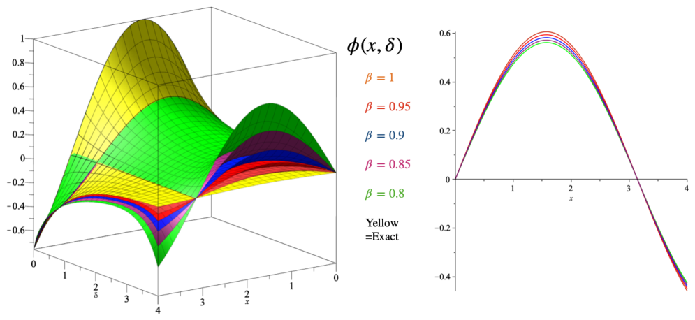
Figure 1 presents the numerical behavior of the solution $\varphi (x,\delta )$ for several fractional orders $\beta =1,0.95,0.90,0.85,$ and $0.80$. The surface plots are illustrated on the computational domain $(x,\delta )\in [0,4]\times [0,4]$, whereas the corresponding 2D cross-sectional curves are depicted at the fixed time level $\delta =0.5$. The results show that the exact solution is recovered when $\beta =1$; also, the results demonstrate the effect of varying the fractional order on the evolution of the solution profile.

Example 2 

([24]). Consider the following system of singular fractional coupled Burgers equations with the initial conditions:

$$\begin{array}{ccc}\hfill D_{\delta }^{\beta }\varphi -{\displaystyle \frac{1}{x}}{\left(x{\varphi }_x\right)}_x-2\varphi {\varphi }_x+{\left(\varphi \omega \right)}_x& =& -x^2{e}^{-\delta }-4e^{-\delta },\hfill \\ \hfill D_{\delta }^{\beta }\omega -{\displaystyle \frac{1}{x}}{\left(x{\omega }_x\right)}_x-2\omega {\omega }_x+{\left(\varphi \omega \right)}_x& =& -x^2{e}^{-\delta }-4e^{-\delta },0<\beta \le 1,\hfill \end{array}$$

(48)

subject to

$$\varphi (x,0)=x^2,\omega (x,0)=x^2.$$

(49)

To solve Equation (48), the following steps are required.

Step 1:  In order to remove the singularity, first we multiply Equation (48) by x; one can obtain

$$\begin{array}{ccc}\hfill x{D}_{\delta }^{\beta }\varphi -{\left(x{\varphi }_x\right)}_x-2x\varphi {\varphi }_x+x{\left(\varphi \omega \right)}_x& =& -x^3{e}^{-\delta }-4x{e}^{-\delta },\hfill \\ \hfill x{D}_{\delta }^{\beta }\omega -{\left(x{\omega }_x\right)}_x-2x\omega {\omega }_x+x{\left(\varphi \omega \right)}_x& =& -x^3{e}^{-\delta }-4x{e}^{-\delta }.\hfill \end{array}$$

(50)

Step 2:  Applying the NGLT to Equation (50) and the NT to Equation (49), we get

$$\begin{array}{ccc}\hfill {\mathrm{N}}^{+}{G}_{\alpha }\left[x{D}_{\delta }^{\beta }\varphi \right]& =& {\mathrm{N}}^{+}{G}_{\alpha }\left[{\left(x{\varphi }_x\right)}_x+2x\varphi {\varphi }_x-x{\left(\varphi \omega \right)}_x\right]\hfill \\ & & -{\mathrm{N}}^{+}{G}_{\alpha }\left[x^3{e}^{-\delta }+4x{e}^{-\delta }\right],\hfill \end{array}$$

(51)

and

$$\begin{array}{ccc}\hfill {\mathrm{N}}^{+}{G}_{\alpha }\left[x{D}_{\delta }^{\beta }\omega \right]& =& {\mathrm{N}}^{+}{G}_{\alpha }\left[{\left(x{\omega }_x\right)}_x+2x\omega {\omega }_x-x{\left(\varphi \omega \right)}_x\right]\hfill \\ & & -{\mathrm{N}}^{+}{G}_{\alpha }\left[x^3{e}^{-\delta }+4x{e}^{-\delta }\right].\hfill \end{array}$$

(52)

Using Theorem 2, the above equations become

$$\begin{array}{ccc}\hfill {\displaystyle \frac{u}{p{s}^{\beta }}}{\displaystyle \frac{d}{du}}\left(u\Phi (p;u,s)\right)& =& {\displaystyle \frac{u{s}^{\alpha -\beta +1}}{p}}{\displaystyle \frac{d}{du}}\left(u\Phi (p;u,0)\right)\hfill \\ & & +{\mathrm{N}}^{+}{G}_{\alpha }\left[{\left(x{\varphi }_x\right)}_x+2x\varphi {\varphi }_x-x{\left(\varphi \omega \right)}_x\right]\hfill \\ & & -{\mathrm{N}}^{+}{G}_{\alpha }\left[\left(x^3+4x\right)\left(1-\delta +{\displaystyle \frac{{\delta }^2}{2!}}-{\displaystyle \frac{{\delta }^3}{3!}}+\dots \right)\right],\hfill \end{array}$$

and

$$\begin{array}{ccc}\hfill {\displaystyle \frac{u}{p{s}^{\beta }}}{\displaystyle \frac{d}{du}}\left(uW(p;u,s)\right)& =& {\displaystyle \frac{u{s}^{\alpha -\beta +1}}{p}}{\displaystyle \frac{d}{du}}\left(uW(p;u,0)\right)\hfill \\ & & +{\mathrm{N}}^{+}{G}_{\alpha }\left[{\left(x{\omega }_x\right)}_x+2x\omega {\omega }_x-x{\left(\varphi \omega \right)}_x\right]\hfill \\ & & -{\mathrm{N}}^{+}{G}_{\alpha }\left[\left(x^3+4x\right)\left(1-\delta +{\displaystyle \frac{{\delta }^2}{2!}}-{\displaystyle \frac{{\delta }^3}{3!}}+\dots \right)\right],\hfill \end{array}$$

where

$$\begin{array}{ccc}\hfill \Phi (p;u,0)& =& {\displaystyle \frac{2!u^2}{p^3}},W(p;u,0)={\displaystyle \frac{2!u^2}{p^3}},\hfill \\ & & {\mathrm{N}}^{+}{G}_{\alpha }\left[\left(x^3+4x\right)\left(1-\delta +{\displaystyle \frac{{\delta }^2}{2!}}-{\displaystyle \frac{{\delta }^3}{3!}}+\dots \right)\right]\hfill \\ & =& \left({\displaystyle \frac{3!u^3}{p^4}}+{\displaystyle \frac{4u}{p^2}}\right)\left(s^{\alpha +1}-s^{\alpha +2}+s^{\alpha +3}-\dots \right).\hfill \end{array}$$

Hence, Equations (51) and (52) can be written as

$$\begin{array}{ccc}\hfill \Phi (p;u,s)& =& {\displaystyle \frac{2!u^2{s}^{\alpha +1}}{p^3}}+{\displaystyle \frac{1}{u}}{\int }_0^u{\displaystyle \frac{p{s}^{\beta }}{u}}{\mathrm{N}}^{+}{G}_{\alpha }\left[\Delta \right]du\hfill \\ & & -{\displaystyle \frac{1}{u}}{\int }_0^u\left({\displaystyle \frac{3!u^2}{p^3}}+{\displaystyle \frac{4}{p}}\right)\left(s^{\alpha +\beta +1}-s^{\alpha +\beta +2}+s^{\alpha +\beta +3}-\dots \right)du,\hfill \end{array}$$

(53)

and

$$\begin{array}{ccc}\hfill W(p;u,s)& =& {\displaystyle \frac{2!u^2{s}^{\alpha +1}}{p^3}}+{\displaystyle \frac{1}{u}}{\int }_0^u{\displaystyle \frac{p{s}^{\beta }}{u}}{\mathrm{N}}^{+}{G}_{\alpha }\left[{\rm Y}\right]du\hfill \\ & & -{\displaystyle \frac{1}{u}}{\int }_0^u\left({\displaystyle \frac{3!u^2}{p^3}}+{\displaystyle \frac{4}{p}}\right)\left(s^{\alpha +\beta +1}-s^{\alpha +\beta +2}+s^{\alpha +\beta +3}-\dots \right)du,\hfill \end{array}$$

(54)

where

$$\begin{array}{ccc}\hfill \Delta & =& {\left(x{\varphi }_x\right)}_x+2x\varphi {\varphi }_x-x{\left(\varphi \omega \right)}_x,\hfill \\ \hfill {\rm Y}& =& {\left(x{\omega }_x\right)}_x+2x\omega {\omega }_x-x{\left(\varphi \omega \right)}_x.\hfill \end{array}$$

Step 3:  Applying the inverse NGLT to Equations (53) and (54), we obtain

$$\begin{array}{ccc}\hfill \varphi (x,\delta )& =& x^2-\left(x^2+4\right)\left({\displaystyle \frac{{\delta }^{\beta }}{\Gamma (\beta +1)}}-{\displaystyle \frac{{\delta }^{\beta +1}}{\Gamma (\beta +2)}}+{\displaystyle \frac{{\delta }^{\beta +2}}{\Gamma (\beta +3)}}-\dots \right)\hfill \\ & & +N^{-1}{G}_s^{-1}\left[{\displaystyle \frac{1}{u}}{\int }_0^u{\displaystyle \frac{p{s}^{\beta }}{u}}{\mathrm{N}}^{+}{G}_{\alpha }\left[\Delta \right]du\right],\hfill \end{array}$$

(55)

and

$$\begin{array}{ccc}\hfill \omega (x,\delta )& =& x^2-\left(x^2+4\right)\left({\displaystyle \frac{{\delta }^{\beta }}{\Gamma (\beta +1)}}-{\displaystyle \frac{{\delta }^{\beta +1}}{\Gamma (\beta +2)}}+{\displaystyle \frac{{\delta }^{\beta +2}}{\Gamma (\beta +3)}}-\dots \right)\hfill \\ & & +N^{-1}{G}_s^{-1}\left[{\displaystyle \frac{1}{u}}{\int }_0^u{\displaystyle \frac{p{s}^{\beta }}{u}}{\mathrm{N}}^{+}{G}_{\alpha }\left[{\rm Y}\right]du\right].\hfill \end{array}$$

(56)

Differentiating Equations (55) and (56) with respect to δ, we get

$$\begin{array}{ccc}\hfill {\displaystyle \frac{\partial \varphi }{\partial \delta }}& +& \left(x^2+4\right)\left({\displaystyle \frac{{\delta }^{\beta -1}}{\Gamma \left(\beta \right)}}-{\displaystyle \frac{{\delta }^{\beta }}{\Gamma (\beta +1)}}+{\displaystyle \frac{{\delta }^{\beta +1}}{\Gamma (\beta +2)}}-\dots \right)\hfill \\ & & -N^{-1}{G}_s^{-1}\left[{\displaystyle \frac{1}{u}}{\int }_0^u{\displaystyle \frac{p{s}^{\beta }}{u}}{\mathrm{N}}^{+}{G}_{\alpha }\left[\Delta \right]du\right]=0,\hfill \end{array}$$

(57)

and

$$\begin{array}{ccc}\hfill {\displaystyle \frac{\partial \omega }{\partial \delta }}& +& \left(x^2+4\right)\left({\displaystyle \frac{{\delta }^{\beta -1}}{\Gamma \left(\beta \right)}}-{\displaystyle \frac{{\delta }^{\beta }}{\Gamma (\beta +1)}}+{\displaystyle \frac{{\delta }^{\beta +1}}{\Gamma (\beta +2)}}-\dots \right)\hfill \\ & & -N^{-1}{G}_s^{-1}\left[{\displaystyle \frac{1}{u}}{\int }_0^u{\displaystyle \frac{p{s}^{\beta }}{u}}{\mathrm{N}}^{+}{G}_{\alpha }\left[{\rm Y}\right]du\right]=0.\hfill \end{array}$$

(58)

According to the VIM, the correction functionals can be constructed as

$$\begin{array}{ccc}\hfill {\varphi }_{n+1}& =& {\varphi }_n+{\int }_0^{\delta }{\lambda }_1\left[{\displaystyle \frac{\partial {\varphi }_n(x,t)}{\partial t}}-{\displaystyle \frac{\partial }{\partial t}}\left(N^{-1}{G}_s^{-1}\left[s^{\beta }{\mathrm{N}}^{+}{G}_{\alpha }\left[{\varphi }_{nxx}-A_n+{\left(C_n\right)}_x\right]\right]\right)\right]dt\hfill \\ & & +{\int }_0^{\delta }{\lambda }_1\left[\left(x^2+4\right)\left({\displaystyle \frac{{\delta }^{\beta -1}}{\Gamma \left(\beta \right)}}-{\displaystyle \frac{{\delta }^{\beta }}{\Gamma (\beta +1)}}+{\displaystyle \frac{{\delta }^{\beta +1}}{\Gamma (\beta +2)}}-\dots \right)\right]dt,\hfill \\ \hfill {\omega }_{n+1}& =& {\omega }_n+{\int }_0^{\delta }{\lambda }_2\left[{\displaystyle \frac{\partial {\omega }_n(x,t)}{\partial t}}-{\displaystyle \frac{\partial }{\partial t}}\left(N^{-1}{G}_s^{-1}\left[s^{\beta }{\mathrm{N}}^{+}{G}_{\alpha }\left[{\omega }_{nxx}-B_n+{\left(C_n\right)}_x\right]\right]\right)\right]dt\hfill \\ & & +{\int }_0^{\delta }{\lambda }_2\left[\left(x^2+4\right)\left({\displaystyle \frac{{\delta }^{\beta -1}}{\Gamma \left(\beta \right)}}-{\displaystyle \frac{{\delta }^{\beta }}{\Gamma (\beta +1)}}+{\displaystyle \frac{{\delta }^{\beta +1}}{\Gamma (\beta +2)}}-\dots \right)\right]dt,\hfill \end{array}$$

(59)

where ${\lambda }_1$ and ${\lambda }_2$ are the Lagrange multipliers determined optimally by the variational theory. The correction functionals for ${\lambda }_1={\lambda }_2=-1$ are obtained using VIM for Equation (59), yielding the recurrence relations

$$\begin{array}{ccc}\hfill {\varphi }_{n+1}& =& {\varphi }_n+{\int }_0^{\delta }\left[-{\displaystyle \frac{\partial {\varphi }_n(x,t)}{\partial t}}+{\displaystyle \frac{\partial }{\partial t}}\left(N^{-1}{G}_s^{-1}\left[s^{\beta }{\mathrm{N}}^{+}{G}_{\alpha }\left[{\varphi }_{nxx}-A_n+{\left(C_n\right)}_x\right]\right]\right)\right]dt\hfill \\ & & -{\int }_0^{\delta }\left(x^2+4\right)\left({\displaystyle \frac{{\delta }^{\beta -1}}{\Gamma \left(\beta \right)}}-{\displaystyle \frac{{\delta }^{\beta }}{\Gamma (\beta +1)}}+{\displaystyle \frac{{\delta }^{\beta +1}}{\Gamma (\beta +2)}}-\dots \right)dt,\hfill \\ \hfill {\omega }_{n+1}& =& {\omega }_n+{\int }_0^{\delta }\left[-{\displaystyle \frac{\partial {\omega }_n(x,t)}{\partial t}}+{\displaystyle \frac{\partial }{\partial t}}\left(N^{-1}{G}_s^{-1}\left[s^{\beta }{\mathrm{N}}^{+}{G}_{\alpha }\left[{\omega }_{nxx}-B_n+{\left(C_n\right)}_x\right]\right]\right)\right]dt\hfill \\ & & -{\int }_0^{\delta }\left(x^2+4\right)\left({\displaystyle \frac{{\delta }^{\beta -1}}{\Gamma \left(\beta \right)}}-{\displaystyle \frac{{\delta }^{\beta }}{\Gamma (\beta +1)}}+{\displaystyle \frac{{\delta }^{\beta +1}}{\Gamma (\beta +2)}}-\dots \right)dt.\hfill \end{array}$$

(60)

The first approximation is

$$\begin{array}{ccc}\hfill {\varphi }_0& =& x^2-\left(x^2+4\right)\left({\displaystyle \frac{{\delta }^{\beta }}{\Gamma (\beta +1)}}-{\displaystyle \frac{{\delta }^{\beta +1}}{\Gamma (\beta +2)}}+{\displaystyle \frac{{\delta }^{\beta +2}}{\Gamma (\beta +3)}}-\dots \right),\hfill \\ \hfill {\omega }_0& =& x^2-\left(x^2+4\right)\left({\displaystyle \frac{{\delta }^{\beta }}{\Gamma (\beta +1)}}-{\displaystyle \frac{{\delta }^{\beta +1}}{\Gamma (\beta +2)}}+{\displaystyle \frac{{\delta }^{\beta +2}}{\Gamma (\beta +3)}}-\dots \right).\hfill \end{array}$$

At $n=0$, we obtain

$$\begin{array}{ccc}\hfill {\varphi }_1& =& {\varphi }_0+{\int }_0^{\delta }\left[-{\displaystyle \frac{\partial {\varphi }_0(x,t)}{\partial t}}+{\displaystyle \frac{\partial }{\partial t}}\left(N^{-1}{G}_s^{-1}\left[s^{\beta }{\mathrm{N}}^{+}{G}_{\alpha }\left[{\varphi }_{0xx}-A_0+{\left(C_0\right)}_x\right]\right]\right)\right]dt\hfill \\ & & -{\int }_0^{\delta }\left(x^2+4\right)\left({\displaystyle \frac{{\delta }^{\beta -1}}{\Gamma \left(\beta \right)}}-{\displaystyle \frac{{\delta }^{\beta }}{\Gamma (\beta +1)}}+{\displaystyle \frac{{\delta }^{\beta +1}}{\Gamma (\beta +2)}}-\dots \right)dt,\hfill \end{array}$$

(61)

and

$$\begin{array}{ccc}\hfill {\omega }_1& =& {\omega }_0+{\int }_0^{\delta }\left[-{\displaystyle \frac{\partial {\omega }_0(x,t)}{\partial t}}+{\displaystyle \frac{\partial }{\partial t}}\left(N^{-1}{G}_s^{-1}\left[s^{\beta }{\mathrm{N}}^{+}{G}_{\alpha }\left[{\omega }_{0xx}-B_0+{\left(C_0\right)}_x\right]\right]\right)\right]dt\hfill \\ & & -{\int }_0^{\delta }\left(x^2+4\right)\left({\displaystyle \frac{{\delta }^{\beta -1}}{\Gamma \left(\beta \right)}}-{\displaystyle \frac{{\delta }^{\beta }}{\Gamma (\beta +1)}}+{\displaystyle \frac{{\delta }^{\beta +1}}{\Gamma (\beta +2)}}-\dots \right)dt.\hfill \end{array}$$

(62)

Substituting ${\varphi }_0$ and ${\omega }_0$ into Equations (61) and (62), respectively, gives

$$\begin{array}{ccc}\hfill {\varphi }_1& =& x^2-\left(x^2+4\right)\left({\displaystyle \frac{{\delta }^{\beta }}{\Gamma (\beta +1)}}-{\displaystyle \frac{{\delta }^{\beta +1}}{\Gamma (\beta +2)}}+{\displaystyle \frac{{\delta }^{\beta +2}}{\Gamma (\beta +3)}}-\dots \right)\hfill \\ & & +{\displaystyle \frac{4{\delta }^{\beta }}{\Gamma (\beta +1)}}-4\left({\displaystyle \frac{{\delta }^{2\beta }}{\Gamma (2\beta +1)}}-{\displaystyle \frac{{\delta }^{2\beta +1}}{\Gamma (2\beta +2)}}+{\displaystyle \frac{{\delta }^{2\beta +2}}{\Gamma (2\beta +3)}}-\dots \right),\hfill \end{array}$$

and

$$\begin{array}{ccc}\hfill {\omega }_1& =& x^2-\left(x^2+4\right)\left({\displaystyle \frac{{\delta }^{\beta }}{\Gamma (\beta +1)}}-{\displaystyle \frac{{\delta }^{\beta +1}}{\Gamma (\beta +2)}}+{\displaystyle \frac{{\delta }^{\beta +2}}{\Gamma (\beta +3)}}-\dots \right)\hfill \\ & & +{\displaystyle \frac{4{\delta }^{\beta }}{\Gamma (\beta +1)}}-4\left({\displaystyle \frac{{\delta }^{2\beta }}{\Gamma (2\beta +1)}}-{\displaystyle \frac{{\delta }^{2\beta +1}}{\Gamma (2\beta +2)}}+{\displaystyle \frac{{\delta }^{2\beta +2}}{\Gamma (2\beta +3)}}-\dots \right).\hfill \end{array}$$

Similarly, at $n=1$, we get

$$\begin{array}{ccc}\hfill {\varphi }_2& =& x^2-\left(x^2+4\right)\left({\displaystyle \frac{{\delta }^{\beta }}{\Gamma (\beta +1)}}-{\displaystyle \frac{{\delta }^{\beta +1}}{\Gamma (\beta +2)}}+{\displaystyle \frac{{\delta }^{\beta +2}}{\Gamma (\beta +3)}}-\dots \right)\hfill \\ & & +{\displaystyle \frac{4{\delta }^{\beta }}{\Gamma (\beta +1)}}-4\left({\displaystyle \frac{{\delta }^{2\beta }}{\Gamma (2\beta +1)}}-{\displaystyle \frac{{\delta }^{2\beta +1}}{\Gamma (2\beta +2)}}+{\displaystyle \frac{{\delta }^{2\beta +2}}{\Gamma (2\beta +3)}}-\dots \right),\hfill \end{array}$$

and

$$\begin{array}{ccc}\hfill {\omega }_2& =& x^2-\left(x^2+4\right)\left({\displaystyle \frac{{\delta }^{\beta }}{\Gamma (\beta +1)}}-{\displaystyle \frac{{\delta }^{\beta +1}}{\Gamma (\beta +2)}}+{\displaystyle \frac{{\delta }^{\beta +2}}{\Gamma (\beta +3)}}-\dots \right)\hfill \\ & & +{\displaystyle \frac{4{\delta }^{\beta }}{\Gamma (\beta +1)}}-4\left({\displaystyle \frac{{\delta }^{2\beta }}{\Gamma (2\beta +1)}}-{\displaystyle \frac{{\delta }^{2\beta +1}}{\Gamma (2\beta +2)}}+{\displaystyle \frac{{\delta }^{2\beta +2}}{\Gamma (2\beta +3)}}-\dots \right).\hfill \end{array}$$

Proceeding similarly for $n=2$, we obtain

$$\begin{array}{ccc}\hfill {\varphi }_3& =& x^2-\left(x^2+4\right)\left({\displaystyle \frac{{\delta }^{\beta }}{\Gamma (\beta +1)}}-{\displaystyle \frac{{\delta }^{\beta +1}}{\Gamma (\beta +2)}}+{\displaystyle \frac{{\delta }^{\beta +2}}{\Gamma (\beta +3)}}-\dots \right)\hfill \\ & & +{\displaystyle \frac{4{\delta }^{\beta }}{\Gamma (\beta +1)}}-4\left({\displaystyle \frac{{\delta }^{2\beta }}{\Gamma (2\beta +1)}}-{\displaystyle \frac{{\delta }^{2\beta +1}}{\Gamma (2\beta +2)}}+{\displaystyle \frac{{\delta }^{2\beta +2}}{\Gamma (2\beta +3)}}-\dots \right),\hfill \end{array}$$

and

$$\begin{array}{ccc}\hfill {\omega }_3& =& x^2-\left(x^2+4\right)\left({\displaystyle \frac{{\delta }^{\beta }}{\Gamma (\beta +1)}}-{\displaystyle \frac{{\delta }^{\beta +1}}{\Gamma (\beta +2)}}+{\displaystyle \frac{{\delta }^{\beta +2}}{\Gamma (\beta +3)}}-\dots \right)\hfill \\ & & +{\displaystyle \frac{4{\delta }^{\beta }}{\Gamma (\beta +1)}}-4\left({\displaystyle \frac{{\delta }^{2\beta }}{\Gamma (2\beta +1)}}-{\displaystyle \frac{{\delta }^{2\beta +1}}{\Gamma (2\beta +2)}}+{\displaystyle \frac{{\delta }^{2\beta +2}}{\Gamma (2\beta +3)}}-\dots \right).\hfill \end{array}$$

Hence, the recurrence relation provides the nth-order approximate solution of Equation (48) as

$$\begin{array}{ccc}\hfill {\varphi }_n& =& x^2-\left(x^2+4\right)\left({\displaystyle \frac{{\delta }^{\beta }}{\Gamma (\beta +1)}}-{\displaystyle \frac{{\delta }^{\beta +1}}{\Gamma (\beta +2)}}+{\displaystyle \frac{{\delta }^{\beta +2}}{\Gamma (\beta +3)}}-\dots \right)\hfill \\ & & +{\displaystyle \frac{4{\delta }^{\beta }}{\Gamma (\beta +1)}}-4\left({\displaystyle \frac{{\delta }^{2\beta }}{\Gamma (2\beta +1)}}-{\displaystyle \frac{{\delta }^{2\beta +1}}{\Gamma (2\beta +2)}}+{\displaystyle \frac{{\delta }^{2\beta +2}}{\Gamma (2\beta +3)}}-\dots \right),\hfill \end{array}$$

(63)

and

$$\begin{array}{ccc}\hfill {\omega }_n& =& x^2-\left(x^2+4\right)\left({\displaystyle \frac{{\delta }^{\beta }}{\Gamma (\beta +1)}}-{\displaystyle \frac{{\delta }^{\beta +1}}{\Gamma (\beta +2)}}+{\displaystyle \frac{{\delta }^{\beta +2}}{\Gamma (\beta +3)}}-\dots \right)\hfill \\ & & +{\displaystyle \frac{4{\delta }^{\beta }}{\Gamma (\beta +1)}}-4\left({\displaystyle \frac{{\delta }^{2\beta }}{\Gamma (2\beta +1)}}-{\displaystyle \frac{{\delta }^{2\beta +1}}{\Gamma (2\beta +2)}}+{\displaystyle \frac{{\delta }^{2\beta +2}}{\Gamma (2\beta +3)}}-\dots \right).\hfill \end{array}$$

(64)

Therefore, as $n\to \infty$, Equations (63) and (64) converge to the exact solution of the time-fractional initial value problem in Equation (48):

$$\varphi (x,\delta )=\underset{n\to \infty }{\lim }{\varphi }_n,\omega (x,\delta )=\underset{n\to \infty }{\lim }{\omega }_n.$$

As the fractional order β approaches 1, the exact solution reduces to

$$\varphi (x,\delta )=x^2{e}^{-\delta },\omega (x,\delta )=x^2{e}^{-\delta }.$$

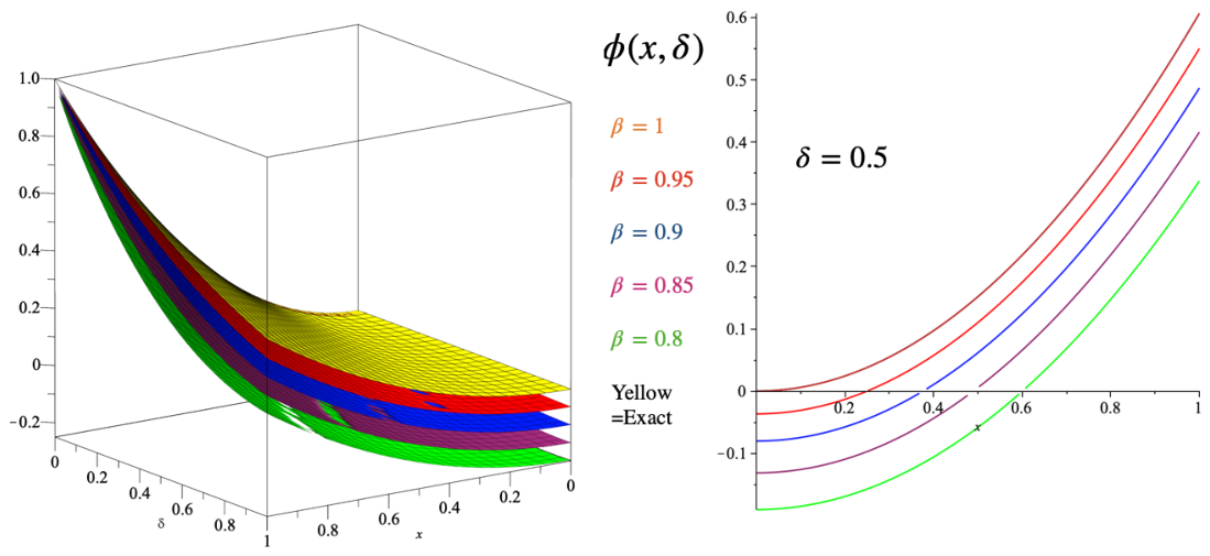
Figure 2 presents a comparison between the exact and numerical solutions of $\varphi (x,\delta ).$ The 3D plots are shown over $x,\delta \in [0,1]$ for different fractional orders $\beta \in \{1,0.95,0.90,0.85,0.80\}$, while the 2D profiles are plotted at $\delta =0.5$. The results indicate that the exact solution is recovered when $\beta =1$, and noticeable deviations appear as β decreases, highlighting the effect of the fractional order.

7. Conclusions

In this paper, we proposed the natural generalized Laplace transform (NGLT) and double natural generalized Laplace transform (DNGLT) as new techniques to get analytical solutions of complex fractional problems, including fractional Burgers equations. We have provided some definitions, theorems, and examples that demonstrate the strength and advantages of these methods. The proposed approach combines the natural generalized Laplace transform with the variational iteration method to develop a new analytical scheme that overcomes the difficulties encountered in solving singular fractional differential equations. The numerical examples of this work confirm the accuracy, reliability, and efficiency of the proposed method (DNGLTVIM). Moreover, the obtained results show that the method gives rapidly convergent series solutions, and it is applicable for linear and nonlinear coupled systems efficiently. In future work, the proposed method (DNGLTVIM) will be extended to explore systems of higher-dimensional singular partial differential equations and other types of nonlinear fractional models.

References

1. Rawashdeh, M.S.; Maitama, S. Solving coupled system of nonlinear PDE’s using the natural decomposition method. Int. J. Pure Appl. Math. 2014, 92, 757–776. [Google Scholar] [CrossRef] [Scilit]
2. Rawashdeh, M.S.; Maitama, S. Solving nonlinear ordinary differential equations using the NDM. J. Appl. Anal. Comput. 2015, 5, 77–88. [Google Scholar] [CrossRef] [Scilit]
3. Cherif, M.H.; Ziane, D.B.K. Fractional natural decomposition method for solving fractional system of nonlinear equations of unsteady flow of a polytropic gas. Nonlinear Stud. 2018, 75, 753–764. [Google Scholar]
4. Shah, R.; Khan, H.; Kumam, P.; Arif, M.; Baleanu, D. Natural Transform Decomposition Method for Solving Fractional-Order Partial Differential Equations with Proportional Delay. Mathematics 2019, 7, 532. [Google Scholar] [CrossRef] [Scilit]
5. Endalew, M.F.; Zhang, X. Application of Modified Laplace Variational Iteration Hybrid Approach for Solving Time-Fractional Fourth-Order Parabolic PDEs. J. Appl. Math. 2025, 2025, 5566075. [Google Scholar] [CrossRef] [Scilit]
6. Handibag, S.S.; Bhosale, J.H. Solution of Nonlinear Integro-Differential Equations by Using Laplace Decomposition Method and Series Solution Method. Indian J. Sci. Technol. 2025, 18, 974–982. [Google Scholar] [CrossRef] [Scilit]
7. Damak, M.; Mohammed, Z.A. Variational Iteration Method for Solving Fractional Integro-Differential Equations with Conformable Differointegration. Axioms 2022, 11, 586. [Google Scholar] [CrossRef] [Scilit]
8. Abolhasani, M.; Abbasbandy, S.A.T. A New Variational Iteration Method for a Class of Fractional Convection-Diffusion Equations in Large Domains. Mathematics 2017, 5, 26. [Google Scholar] [CrossRef] [Scilit]
9. Brociek, R.; Pleszczyński, M. Differential Transform Method (DTM) and Physics-Informed Neural Networks (PINNs) in Solving Integral–Algebraic Equation Systems. Symmetry 2024, 16, 1619. [Google Scholar] [CrossRef] [Scilit]
10. Brociek, R.; Wajda, A.; Napoli, C.; Capizzi, G.; Słota, D. An Inverse Problem for a Fractional Space–Time Diffusion Equation with Fractional Boundary Condition. Entropy 2026, 28, 81. [Google Scholar] [CrossRef] [Scilit] [PubMed]
11. Abusaleh, G.; Ullaha, M.A. Fractional Differential Equations and Its Solutions Using the Laplace Variational Iteration Method. GANIT J. Bangladesh Math. Soc. 2025, 45, 31–44. [Google Scholar] [CrossRef] [Scilit]
12. Singh, G.; Singh, I.; AlDerea, A.M.; Alanzi, A.M.; Khalifa, H.A.E.W. Solutions of (2+1)-D and (3+1)-D Burgers Equations by New Laplace Variational Iteration Technique. Axioms 2023, 12, 647. [Google Scholar] [CrossRef] [Scilit]
13. Eltayeb, H.; Aldossari, S. Solution of Time-Fractional Partial Differential Equations via the Natural Generalized Laplace Transform Decomposition Method. Fractal Fract. 2025, 9, 554. [Google Scholar] [CrossRef] [Scilit]
14. Nazneen, A.; Ali, N.; Hussain, S.M.; Ahmad, H.; Nawaz, R.; Zada, L.; Irfan, R.; Guedri, K.; Almaliki, A.H.; Bayram, M. Fractional Analysis of Benjamin–Bona–Mahony Equation Across Natural Transform Iterative Method: Thermal Engineering Implementations. Sci. Rep. 2025, 15, 20082. [Google Scholar] [CrossRef] [Scilit] [PubMed]
15. Bushnaq, S.; Ali, A.; Abdullah. Numerical Investigation of the Fractional Fisher Partial Differential Equation via Natural Transform Decomposition Method. Partial. Differ. Equ. Appl. Math. 2024, 9, 100642. [Google Scholar] [CrossRef] [Scilit]
16. Agarwal, R.P.; Mofarreh, F.; Shah, R.; Luangboon, W.; Nonlaopon, K. An Analytical Technique Based on Natural Transform to Solve Fractional-Order Parabolic Equations. Entropy 2021, 23, 1086. [Google Scholar] [CrossRef] [Scilit] [PubMed]
17. Haq, I.U.; Ullah, Z. Natural Decomposition Method and Coupled Systems of Nonlinear Fractional-Order Partial Differential Equations. Results Nonlinear Anal. 2020, 3, 35–44. [Google Scholar] [CrossRef] [Scilit]
18. Sattaso, S.; Nonlaopon, K.; Kim, H. Further properties of laplace-type integral transforms. Dyn. Syst. Appl. 2019, 28, 195–215. [Google Scholar]
19. Bayrak, M.; Demir, A. A New Approach for Space-Time Fractional Partial Differential Equations by Residual Power Series Method. Appl. Math. Comput. 2018, 336, 215–230. [Google Scholar] [CrossRef] [Scilit]
20. Jachymski, J.; Iżwik, I.; Terepeta, M. The Banach Fixed Point Theorem: Selected Topics from Its Hundred-Year History. Rev. Real Acad. Cienc. Exactas Fís. Nat. Ser. A Mat. 2024, 118, 140. [Google Scholar] [CrossRef] [Scilit]
21. Khan, H.; Khan, A.; Chen, W.; Shah, K. Stability analysis and a numerical scheme for fractional Klein-Gordon equations. Math. Methods Appl. Sci. 2019, 42, 723–732. [Google Scholar] [CrossRef] [Scilit]
22. Eltayeb, H. Application of Natural Generalized-Laplace Transform and Its Properties. Mathematics 2025, 13, 1394. [Google Scholar] [CrossRef] [Scilit]
23. Park, S. Revisit to Suzuki’s Metric Completeness. Nonlinear Convex Anal. Optim. 2024, 3, 47–62. [Google Scholar]
24. Eltayeb, H.; Mesloub, S. Solution for Time-Fractional Coupled Burgers Equations by Generalized Laplace Transform Methods. Fractal Fract. 2024, 8, 692. [Google Scholar] [CrossRef] [Scilit]
Figure 1. Three-dimensional surface and two-dimensional sectional plots of the solution ϕ ( x , δ ) for various fractional orders β { 1 , 0.95 , 0.90 , 0.85 , 0.80 } . The 3D surfaces are presented over the domain ( x , δ ) [ 0 , 4 ] × [ 0 , 4 ] , while the corresponding 2D profiles are displayed at the fixed value δ = 0.5 , showing the effect of the fractional order on the solution behavior.
Mathematics 14 02381 g001
Figure 2. Three-dimensional surface and two-dimensional sectional plots of the solution ϕ ( x , δ ) for various fractional orders β { 1 , 0.95 , 0.90 , 0.85 , 0.80 } . The 3D plot is generated over the domain x , δ [ 0 , 1 ] , while the 2D profiles correspond to the fixed value δ = 0.5 , highlighting the influence of the fractional order on the dynamics of the solution.
Mathematics 14 02381 g002
Disclaimer/Publisher’s Note: The statements, opinions and data contained in all publications are solely those of the individual author(s) and contributor(s) and not of MDPI and/or the editor(s). MDPI and/or the editor(s) disclaim responsibility for any injury to people or property resulting from any ideas, methods, instructions or products referred to in the content.