An Accelerated Residual ADI Method for Large-Scale Low-Rank Riccati Equations

Abstract

This paper considers the acceleration of the residual alternating direction implicit (RADI) iteration for solving large-scale low-rank Riccati matrix equations arising from time-invariant control systems. A direct attempt to accelerate the ADI iteration by treating the feedback gain matrix as a fixed-point iterate typically leads to a relatively slow convergence of the norm of the residual matrix. To address this issue, we combine the feedback gain matrix with the residual matrix as the input of the RADI iteration and develop an accelerated RADI scheme based on this reformulation. The convergence of the accelerated RADI algorithm is established under a relatively mild assumption. Numerical experiments from engineering applications demonstrate that the proposed accelerated RADI algorithm with properly selected parameters is able to attain a prescribed residual level with fewer iterations and less computational time than the RADI method.

1. Introduction

Consider the continuous-time linear time-invariant (LTI) control system, which has extensive applications in mechanical engineering, electrical and electronic engineering, and aerospace

$$\begin{array}{c}\hfill \dot{x}(t)=Ax(t)+Bu(t),y(t)=Cx(t),\end{array}$$

(1)

where $A\in {\mathbb{C}}^{N\times N}$, $B\in {\mathbb{C}}^{N\times m}$, $C\in {\mathbb{C}}^{p\times N}$ with $m,p\ll N$. We denote by ${\mathbb{C}}^{n\times l}$ the set of complex matrices of size $m\times l$. The linear quadratic regulator (LQR) problem for the LTI system consists of minimizing the cost functional

$$\begin{array}{c}\hfill J_c(x,u)\equiv {\int }_0^{\infty }\left[x{(t)}^{\top }Qx(t)+u{(t)}^{\top }u(t)\right]dt\end{array}$$

(2)

with $Q=C^{*}C$. The optimal control law is given in state-feedback form $u(t)=F_{c}x(t)$, with feedback gain

$$\begin{array}{c}\hfill F_c=-B^{*}{X}_s,\end{array}$$

(3)

where $X_s$ denotes the unique positive semidefinite stabilizing solution of the continuous-time algebraic Riccati equation (CARE)

$$\begin{array}{c}\hfill \mathcal{C}(X)=A^{*}X+XA-XGX+Q=0\end{array}$$

(4)

with $G=B{B}^{*}$ [1].

For large-scale CARE (4) with inherent low-rank structures, a wide range of numerical methods has been developed. Prominent approaches include (inexact) Newton-type methods, where each step requires the solution of a Lyapunov equation typically handled by ADI iterations [2,3,4]; structure-preserving doubling algorithms (SDA), which iteratively expand invariant subspaces associated with structured Hamiltonian matrices [5,6,7,8]; and Krylov subspace methods [9,10,11,12,13,14,15,16], which construct reduced-order projected problems whose solutions approximate that of the original large-scale equation. Similar methods have been applied to other equations; see [17,18] and references therein. Comprehensive numerical comparisons of these methods can be found in [19], indicating that the residual ADI (RADI) method [20] exhibits particularly favorable performance on a variety of practical engineering problems. The central idea of RADI is to represent the residual as a low-rank matrix equation and to update it iteratively via a quadratic ADI scheme. In contrast to many competing methods that progressively enlarge the dimension of the underlying low-rank subspace, RADI maintains a fixed subspace dimension throughout the iteration. This feature yields a significant computational advantage, especially in large-scale settings.

This paper aims to accelerate RADI by exploiting derived residual information from previous iteration steps. A straightforward idea is to apply the Anderson acceleration strategy [21,22,23,24] to the matrix sequence generated by the QADI iteration, namely, the sequence of feedback gain matrices. However, in the low-rank RADI iteration scheme, both the feedback gain matrix and the low-rank factor matrices of the CARE residual need to be updated at each step. In this setting, accelerating only the feedback gain matrix would result in the loss of information contained in the residual factor matrices, thereby leading to relatively slow convergence. In this work, we approach the acceleration of RADI (ARADI) from a different perspective. The main motivations and contributions are summarized as follows:

• The feedback gain matrix and the residual matrix are combined into a unified iterate. The RADI iteration is then reformulated as a nonlinear mapping of this augmented matrix, thereby yielding the corresponding fixed-point framework. By utilizing the previous t iterates together with information from the residual matrix, the combined matrix is updated, leading to an accelerated residual reduction.
• Under the mild assumption that the closed-loop matrix plus the ADI shift remains uniformly bounded in a neighborhood of the stabilizing solution, we establish key properties of the nonlinear function and its Fréchet derivative induced by RADI. These results provide the foundation for proving the local convergence of the proposed accelerated RADI iteration applied to the augmented matrix consisting of the feedback gain and residual matrices.
• Extensive numerical experiments on a variety of practical engineering problems are implemented to compare the RADI method with the proposed safeguarded ARADI (SARADI) algorithm and its simplified variant (ARADI) in terms of iteration counts and computational time. The results demonstrate that, with suitable parameter choices, both SARADI and ARADI attain the prescribed residual tolerance using fewer iterations and less computational effort. In particular, ARADI exhibits the best performance among all approaches.

The remainder of this paper is organized as follows. In Section 2, the iterate scheme of ARADI is introduced, and the associated properties of the nonlinear mapping induced by ARADI are analyzed. Section 3 is devoted to the local convergence theory of the ARADI iteration. In Section 4, the practical safeguarded ARADI framework is presented in detail, and the numerical comparisons among RADI, SARADI, and ARADI are provided for practical engineering problems, demonstrating that, under suitable parameter settings, the proposed ARADI outperforms the other methods both in iteration count and computational time.

Throughout this paper, $I_m$ (or simply I) is the $m\times m$ identity matrix. For a matrix $A\in {\mathbb{C}}^{N\times N}$, $\sigma (A)$ and $\rho (A)$ are the spectrum and the spectral radius of A, respectively. The notations tr(A) and vec(A) represent the trace and the stacked column vector of A, respectively. The matrix $A\in {\mathbb{C}}^{N\times N}$ is c-stable if all eigenvalues of A lie in the open left-half complex plane. Unless stated otherwise, the norm $\parallel ·\parallel$ is the Frobenius norm of a matrix. For matrices A and $B\in {\mathbb{C}}^{N\times N}$, the direct sum $A\oplus B$ means the block diagonal matrix $\left[\begin{array}{cc}A& 0\\ 0& B\end{array}\right]$. We also require the following basic lemma.

Lemma 1

(Banach Lemma [25]). Let A be a nonsingular matrix and E be the perturbation matrix. If $\parallel A^{-1}E\parallel < 1$, then $A+E$ is nonsingular and

$${\parallel (A+E)}^{-1}\parallel \le {\displaystyle \frac{\parallel A^{-1}\parallel }{1 - \parallel A^{-1}E\parallel }}.$$

We also use the following elementary result.

Lemma 2.

Let $M={[A^{*},B^{*}]}^{*}$. The Frobenius norm of M satisfies

$${\displaystyle \frac{1}{\sqrt{2}}}(\parallel A\parallel +\parallel B\parallel )\le \parallel M\parallel \le \parallel A\parallel +\parallel B\parallel .$$

2. Accelerated Residual ADI Method and Preliminaries

In this section, we begin by reviewing the framework of RADI and develop an accelerated RADI strategy for solving CARE (4). We then present several useful properties that underpin the local convergence analysis in Section 3.

2.1. Iteration Format and Acceleration Scheme

Given the initial approximation $X_0=0$, the iteration scheme of quadratic ADI (QADI) [26,27] is

$$\left\{\begin{array}{cc}& X_{1+1/2}\left(A^{*}+{\overline{\sigma }}_{k+1}I-G{X}_k\right)=-Q-(A^{*}+{\overline{\sigma }}_{k+1}I)X_k,\hfill \\ & \left(A^{*}+{\sigma }_{k+1}I-X_{k+1/2}G\right)=-Q-X_{k+1/2}(A-{\sigma }_{k+1}I),\hfill \end{array}\right.$$

where ${\overline{\sigma }}_{k+1}$ is the complex conjugate number of the ADI shift parameter ${\sigma }_{k+1}$ belonging to the left-half complex plane. The convergence of the sequence $\left\{X_k\right\}$ generated by the QADI iteration to the stabilizing solution is generally associated with the eigenvalues of the closed-loop matrix in the LTI system and the given ADI parameters, as summarized in the following theorem [26].

Theorem 1.

Let $X_s$ be the stabilizing solution to CARE (4), that is, the spectrum of the closed-loop matrix $\tilde{A}=A-G{X}_s$ lies in the left-half complex plane. Then, the sequence $\left\{X_k\right\}$ generated by QADI converges to the stabilizing solution $X_s$ with

$$\begin{array}{c}\hfill \parallel X_k-X_s\parallel \le C\left({\displaystyle \underset{{\lambda }_i\in \sigma (\tilde{A})}{max}}{\displaystyle \prod _k}\left|{\displaystyle \frac{({\overline{\sigma }}_k-{\lambda }_i)({\sigma }_k-{\lambda }_i)}{({\sigma }_k+{\lambda }_i)({\overline{\sigma }}_k+{\lambda }_i)}}\right|\right).\end{array}$$

When $G=B{B}^{*}$ and $Q=C^{*}C$ are of the low-ranked form in CARE (4), the QADI iteration can be implemented in an economic low-rank way, referred to as residual ADI (RADI) [20]

$$\left\{\begin{array}{cc}& R_0=C^{*};\hfill \\ & V_{k+1}=\sqrt{-2Re({\sigma }_{k+1})}{(A^{*}-X_{k}B{B}^{*}+{\sigma }_{k+1}I)}^{-1}{R}_k;\hfill \\ & {\tilde{Y}}_{k+1}=I_p-{\displaystyle \frac{1}{2Re({\sigma }_{k+1})}}\left(V_{k+1}^{*}B\right){\left(V_{k+1}^{*}B\right)}^{*};Y_{k+1}=Y_k\oplus {\tilde{Y}}_{k+1};\hfill \\ & R_{k+1}=R_k+\sqrt{-2Re({\sigma }_{k+1})}{V}_{k+1}{\tilde{Y}}_{k+1}^{-1};\hfill \\ & Z_{k+1}=[Z_k,V_{k+1}],\hfill \end{array}\right.$$

(5)

where $\mathrm{Re}(·)$ is the real part of the complex number. The solution to CARE (4), upon termination, is readily approximated by $X_{k+1}=Z_{k+1}{Y}_{k+1}^{-1}{Z}_{k+1}^{*}$ or an equivalent form (with the help of $Z_k$ in (5))

$$\begin{array}{c}\hfill X_{k+1}=X_k+V_{k+1}{\tilde{Y}}_{k+1}^{-1}{V}_{k+1}^{*}.\end{array}$$

Consequently, the equation residual admits a low-ranked form $\mathcal{C}(X_{k+1})=R_{k+1}{R}_{k+1}^{*}$. One merit of RADI, compared with other solution methods [2,3,4,5,6,7,8,9,10,11,12,13,14,15,16], is that the low-rank factor $V_k$ and the residual factor $R_k$ can progress in a fixed column dimension, so it achieves the approximated feedback gain (actually $-F_c^{*}$ in (3))

$$\begin{array}{c}\hfill K_{k+1}=K_k+(V_{k+1}{\tilde{Y}}_{k+1}^{-1})(V_{k+1}^{*}B).\end{array}$$

(6)

To accelerate the RADI with the previously derived residuals using the idea presented in [21,24], an intuition is to regard current $X_k$ generated by QADI (or equivalently $K_k$ of (6) generated by (5)) as a fixed point to construct residual information for updating the next iterate $X_{k+1}$ (or equivalently $K_{k+1}$). However, the norm of the residual factor $R_k$ in this way will stay stagnant, and the accelerated iteration seems divergent. To conquer this deficiency, we combine the current feedback gain $K_k$ with the residual $R_k$ and construct ${\Phi }_k={[K_k^{*},R_k^{*}]}^{*}$. We then take the RADI iteration as a nonlinear function $F({\Phi }_k)$ and record the next residual

$$\begin{array}{c}\hfill F({\Phi }_k)-{\Phi }_k:=U_{k+1}.\end{array}$$

Then, with the information obtained from previous t residuals, we find

$$\begin{array}{c}\hfill {\displaystyle \underset{\alpha }{min}}∥{\displaystyle \sum _{j=k-t}^k}{\displaystyle {\alpha }_j^{(k+1)}}{U}_{j+1}∥\end{array}$$

(7)

such that ${\sum }_{j=k-t+1}^k{\alpha }_j^{(k+1)}=1$. The updated iteration is as follows:

$$\begin{array}{cc}& {\Phi }_{k+1}={\displaystyle \sum _{j=k-t}^k}{\alpha }_j^{(k+1)}{\Phi }_j+\gamma \left({\displaystyle \sum _{j=k-t}^k}{\alpha }_j^{(k+1)}{U}_{j+1}\right),\hfill \end{array}$$

where $0<\gamma \le 1$ is a damper factor.

The practical implementation of the above acceleration in fact proceeds with the approximated feedback gain $K_k$ and the residual $R_k$ and is described in detail in Section 4.

2.2. Properties of $F(\Phi )$

In this subsection, we provide some properties of $F(\Phi )$ that underpin the convergence of the developed ARADI algorithm. For simplicity, we omit the subscript k of the RADI iteration.

Assumption 1.

Let $M(K):=A^{*}-K{B}^{*}+\sigma I$ with ADI shift parameter σ being selected such that $\parallel M^{-1}(K)\parallel$ is uniformly bounded in the neighborhood of solution $X_s$ to (4).

Remark 1.

Assumption 1 is essential for the local convergence analysis of the accelerated RADI (ARADI) method. Under this assumption, both K and R remain bounded provided X is sufficiently close to the stabilizing solution $X_s$. In fact, let

$$K_s=X_{s}B,M_s=A^{*}-K_s{B}^{*}+\sigma I.$$

Since $X_s$ is the stabilizing solution of the CARE and σ is chosen from the admissible shift region, $M_s$ is nonsingular. For any feedback gain K in a neighborhood of $K_s$, we have

$$M(K)=M_s-(K-K_s)B^{*}.$$

If $\parallel M_s^{-1}(K-K_s)B^{*}\parallel < 1$, then $M(K)$ is invertible, and the Banach perturbation lemma yields

$$M{(K)}^{-1}={\left(I-M_s^{-1}(K-K_s)B^{*}\right)}^{-1}{M}_s^{-1},$$

which implies the bound

$${\parallel M(K)}^{-1}\parallel \le {\displaystyle \frac{\parallel M_s^{-1}\parallel }{1 - \parallel M_s^{-1}(K-K_s)B^{*}\parallel }}.$$

In particular, for any $0 < \eta < 1$, the condition

$$\parallel K - K_s\parallel < r_{\eta }:={\displaystyle \frac{\eta }{\parallel M_s^{-1}\parallel \parallel B\parallel }}$$

defines a sufficient neighborhood scope in which the uniform boundedness assumption holds. This estimate explains when the assumption is satisfied and provides a conservative quantitative lower bound for the neighborhood.

Let

$$\begin{array}{c}\hfill V(K,R)=\eta M^{-1}(K)R,W(K,R)={\left(V(K,R)\right)}^{*}B\end{array}$$

with $\eta =\sqrt{-2\mathrm{Re}(\sigma )}$. It is obvious from Assumption 1 that

$$\begin{array}{c}\hfill \parallel V(K,R)\parallel = \parallel \eta M^{-1}(K)R\parallel \le C,\parallel W(K,R)\parallel = \parallel {\left(V(K,R)\right)}^{*}R\parallel \le C,\end{array}$$

(8)

where the constant C is independent of K and R. Moreover, the convergence of the residual factor R in (5), together with Lemma 1, indicates that

$$\begin{array}{c}\hfill \parallel {\tilde{Y}}^{-1}(K,R)\parallel \le {\displaystyle \frac{1}{1-\theta \parallel (W(K,R)W^{*}(K,R)\parallel }} \le C\end{array}$$

(9)

with $\theta ={\displaystyle \frac{1}{2\mathrm{Re}(\sigma )}}$.

Now, for sufficiently small $H={[H_K^{*},H_R^{*}]}^{*}$, by using Lemma 1 again, one also has the bounds

$$\begin{array}{c}\hfill \parallel M^{-1}(K+H_K)\parallel \le C\end{array}$$

(10)

and

$$\begin{array}{c}\hfill \parallel V(K+H_K,R+H_R)\parallel \le C,\parallel {\tilde{Y}}^{-1}(K+H_K,R+H_R)\parallel \le C,\end{array}$$

(11)

where the constant C is independent of K and R. Furthermore, we have the difference bounds

$$\begin{array}{c}\hfill \parallel M{(K+H_K)}^{-1}-M{(K)}^{-1}\parallel \le \parallel M^{-1}(K+H_K)(H_K{B}^{*})M^{-1}(K)\parallel \le C\parallel H_k\parallel \end{array}$$

and

$$\begin{array}{cc}& \parallel V(K+H_K,R+H_R)-V(K,R)\parallel \hfill \\ \le & C(\parallel M^{-1}(K+H_K)-M^{-1}(K)\parallel ·\parallel R\parallel + \parallel M^{-1}(K+H_K)\parallel ·\parallel H_R\parallel )\hfill \\ \le & C_1\parallel H_K\parallel ·\parallel R\parallel + C_2\parallel H_R\parallel \le C(\parallel H_K\parallel + \parallel H_R\parallel ).\hfill \end{array}$$

(12)

These two inequalities, together with (9)–(11), yield

$$\begin{array}{cc}& \parallel \tilde{Y}(K+H_K,R+H_R)-\tilde{Y}(K,R)\parallel \hfill \\ & \le |\theta |\parallel W(K+H_K,R+H_R){\left(W(K+H_K,R+H_R)\right)}^{*}-W(K,R){\left(W(K,R)\right)}^{*}\parallel \hfill \\ & \le C(\parallel W(K+H_K,R+H_R)-W(K,R)\parallel ·\parallel B\parallel ·\parallel V(K+H_K,R+H_R)\parallel \hfill \\ & +\parallel V(K,R)\parallel ·\parallel B\parallel ·\parallel W(K+H_K,R+H_R)-W(K,R)\parallel )\hfill \\ & \le C(\parallel H_K\parallel + \parallel H_R\parallel ).\hfill \end{array}$$

and

$$\begin{array}{cc}& \parallel {\tilde{Y}}^{-1}(K+H_K,R+H_R)-{\tilde{Y}}^{-1}(K,R)\parallel \hfill \\ \le & \parallel {\tilde{Y}}^{-1}(K+H_K,R+H_R)\parallel ·\parallel \tilde{Y}(K+H_K,R+H_R)-\tilde{Y}(K,R)\parallel ·\parallel {\tilde{Y}}^{-1}(K,R)\parallel \hfill \\ \le & C(\parallel H_K\parallel + \parallel H_R\parallel ).\hfill \end{array}$$

(13)

Given $\Phi ={[K^{*},R^{*}]}^{*}$ and the direction $\Psi ={[{\Psi }_K^{*},{\Psi }_R^{*}]}^{*}$, it follows from Assumption 1 that the Fréchet derivative of $V^{\prime }(K,R)$ satisfies

$$\begin{array}{cc}& \parallel V^{\prime }(K,R)\parallel = \parallel \eta M^{-1}(K){\Psi }_R+M^{-1}(K){\Psi }_K{B}^{*}{M}^{-1}(K)R\parallel \hfill \\ & \le C(\parallel M^{-1}(K)\parallel ·\parallel {\Psi }_R\parallel + \parallel M^{-1}(K)\parallel ·\parallel {\Psi }_K\parallel ·\parallel M^{-1}(K)R\parallel )\hfill \\ & \le C(\parallel {\Psi }_K\parallel + \parallel {\Psi }_R\parallel ).\hfill \end{array}$$

(14)

and

$$\begin{array}{cc}& \parallel {\tilde{Y}}^{\prime }(K,R)\parallel = \parallel \theta {\left(V^{\prime }(K,R)\right)}^{*}BW(K,R)+W^{*}(K,R)B^{*}{V}^{\prime }(K,R))\parallel \hfill \\ & \le C(\parallel V^{\prime }(K,R)\parallel ·\parallel W(K,R)\parallel )\hfill \\ & \le C(\parallel {\Psi }_K\parallel + \parallel {\Psi }_R\parallel ).\hfill \end{array}$$

(15)

With a sufficiently small increment H and in a similar way, we can also bound the Fréchet derivatives as

$$\begin{array}{c}\hfill \parallel V^{\prime }(K+H_K,R+H_R)\parallel \le C(\parallel {\Psi }_K\parallel +\parallel {\Psi }_R\parallel ),\parallel {\tilde{Y}}^{\prime }(K+H_K,R+H_R)\parallel \le C(\parallel {\Psi }_K\parallel +\parallel {\Psi }_R\parallel ).\end{array}$$

(16)

Then the difference of the derivative of $V(K,R)$ is bounded by

$$\begin{array}{cc}& \parallel V^{\prime }(K+H_K,R+H_R)-V^{\prime }(K,R)\parallel \hfill \\ \hfill \le & |\eta |·\parallel M^{-1}(K+H_k){\Psi }_R+M^{-1}(K+H_k){\Psi }_K{B}^{*}{M}^{-1}(K+H_k)(R+H_R)\hfill \\ & -M^{-1}(K){\Psi }_R-M^{-1}(K){\Psi }_K{B}^{*}{M}^{-1}(K)R\parallel \hfill \\ \hfill \le & |\eta |·\parallel M^{-1}(K+H_k)-M^{-1}(K)\parallel (\parallel {\Psi }_R\parallel +\parallel {\Psi }_K{B}^{*}{M}^{-1}(K+H_k)(R+H_R)\parallel \hfill \\ & +\parallel M^{-1}(K){\Psi }_K{B}^{*}\parallel ·\parallel R+H_R\parallel )+|\eta |·\parallel M^{-1}(K){\Psi }_K{B}^{*}\parallel ·\parallel M^{-1}(K)\parallel ·\parallel H_R\parallel \parallel \hfill \\ \hfill \le & C\parallel H_R\parallel (\parallel {\Psi }_K\parallel +\parallel {\Psi }_R\parallel ).\hfill \end{array}$$

(17)

This, together with (12), directly yields

$$\begin{array}{cc}& \parallel {\tilde{Y}}^{\prime }(K+H_K,R+H_R)-{\tilde{Y}}^{\prime }(K,R)\parallel \hfill \\ \hfill \le & |\theta |·\parallel {\left(V^{\prime }(K+H_K,R+H_R)\right)}^{*}BW(K+H_K,R+H_R)\hfill \\ & +W^{*}(K+H_K,R+H_R)B^{*}(V^{\prime }(K+H_K,R+H_R)\hfill \\ & -{\left(V^{\prime }(K,R)\right)}^{*}BW(K,R)-W^{*}(K,R)B^{*}{V}^{\prime }(K,R)\parallel \hfill \\ \hfill \le & C_1\parallel V^{\prime }(K+H_K,R+H_R)-V^{\prime }(K,R)\parallel ·\parallel W(K+H_K,R+H_R)\parallel \hfill \\ & +C_2\parallel V^{\prime }(K,R)\parallel ·\parallel W(K+H_K,R+H_R)-W(K,R)\parallel \hfill \\ \hfill \le & C(\parallel H_K\parallel +\parallel H_R\parallel )(\parallel {\Psi }_K\parallel +\parallel {\Psi }_R\parallel ).\hfill \end{array}$$

(18)

Lemma 3.

Under Assumption 1, we have the following properties of RADI iteration $F(\Phi )$ and its derivative $F_{\Phi }^{\prime }(\Psi )$:

(a) 

$\parallel F(\Phi +H)-F(\Phi )\parallel \le C(\parallel H_K\parallel +\parallel H_R\parallel )$;

(b) 

$\parallel F_{\Phi }^{\prime }(\Psi )\parallel \le C(\parallel {\Psi }_K\parallel + \parallel {\Psi }_R\parallel )$;

(c) 

$\parallel F_{\Phi +H}^{\prime }(\Psi )-F_{\Phi }^{\prime }(\Psi )\parallel \le C(\parallel {\Psi }_K\parallel + \parallel {\Psi }_R\parallel )(\parallel H_K\parallel + \parallel H_R\parallel )$;

(d) 

$\parallel F(\Phi +H)-F(\Phi )-F_{\Phi }^{\prime }(H)\parallel \le C(\parallel H_K\parallel + \parallel H_R{\parallel )}^2$.

Proof. 

(a). From (8), (9), (11)–(13), one has

$$\begin{array}{cc}& \parallel V(K+H_K,R+H_R){\tilde{Y}}^{-1}(K+H_K,R+H_R)-V(K,R){\tilde{Y}}^{-1}(K,R)\parallel \hfill \\ \hfill \le & \parallel V(K+H_K,R+H_R)-V(K,R)\parallel ·\parallel {\tilde{Y}}^{-1}(K+H_K,R+H_R)\parallel \hfill \\ & +\parallel V(K,R)\parallel ·\parallel {\tilde{Y}}^{-1}(K+H_K,R+H_R)-{\tilde{Y}}^{-1}(K,R)\parallel \hfill \\ \hfill \le & C(\parallel H_K\parallel +\parallel H_R\parallel )\hfill \end{array}$$

and

$$\begin{array}{cc}& \parallel V(K+H_K,R+H_R){\tilde{Y}}^{-1}(K+H_K,R+H_R)V(K+H_K,R+H_R)\hfill \\ & -V(K,R){\tilde{Y}}^{-1}(K,R)V(K,R)\parallel \hfill \\ \hfill \le & \parallel V(K+H_K,R+H_R)-V(K,R)\parallel ·\parallel {\tilde{Y}}^{-1}(K+H_K,R+H_R)\parallel ·\parallel V(K+H_K,R+H_R)\parallel \hfill \\ & +\parallel V(K,R)\parallel ·\parallel {\tilde{Y}}^{-1}(K+H_K,R+H_R)-{\tilde{Y}}^{-1}(K,R)\parallel ·\parallel V(K+H_K,R+H_R)\parallel \hfill \\ & +\parallel V(K,R)\parallel ·\parallel {\tilde{Y}}^{-1}(K,R)\parallel ·\parallel V(K+H_K,R+H_R)-V(K,R)\parallel \hfill \\ \hfill \le & C(\parallel H_K\parallel +\parallel H_R\parallel ).\hfill \end{array}$$

Therefore,

$$\begin{array}{cc}& \parallel F(X+H)-F(X)\parallel \hfill \\ & =∥\left[\begin{array}{c}{H}_K+V(K+H_K,R+H_R){\tilde{Y}}^{-1}(K+H_K,R+H_R)V(K+H_K,R+H_R)-V(K,R){\tilde{Y}}^{-1}(K,R)V(K,R)\\ H_R+\eta \left(V(K+H_K,R+H_R){\tilde{Y}}^{-1}(K+H_K,R+H_R)-V(K,R){\tilde{Y}}^{-1}(K,R)\right)\end{array}\right]∥\hfill \\ & \le C_1\parallel H_K\parallel +C_2\parallel H_R\parallel +C_3(\parallel H_K\parallel +\parallel H_R\parallel )\hfill \\ & \le C(\parallel H_K\parallel +\parallel H_R\parallel ),\hfill \end{array}$$

where the constants $C_1$, $C_2$, $C_3$, and C are independent of K and R.

(b). It follows from (8), (9), (14), and (15) that

$$\begin{array}{cc}& \parallel F_{{\Phi }_K}^{\prime }(\Psi )\parallel =\parallel {\left(K+V(K,R){\tilde{Y}}^{-1}(K,R)W(K,R)\right)}^{\prime }\parallel \hfill \\ & = \parallel {\Psi }_K+V^{\prime }(K,R){\tilde{Y}}^{-1}(K,R)W(K,R))\hfill \\ & +V(K,R){\tilde{Y}}^{-1}(K,R){\tilde{Y}}^{\prime }(K,R){\tilde{Y}}^{-1}(K,R)W(K,R)\hfill \\ & +V(K,R){\tilde{Y}}^{-1}(K,R){\left(V^{\prime }(K,R)\right)}^{*}B\parallel \hfill \\ & \le \parallel {\Psi }_K\parallel +C(\parallel {\Psi }_K\parallel +\parallel {\Psi }_R\parallel )\hfill \\ & \le C(\parallel {\Psi }_K\parallel +\parallel {\Psi }_R\parallel ).\hfill \end{array}$$

and

$$\begin{array}{cc}& \parallel F_{{\Phi }_R}^{\prime }(\Psi )\parallel =\parallel {\left(R+\eta V(K,R){\tilde{Y}}^{-1}(K,R)\right)}^{\prime }\parallel \hfill \\ & = \parallel {\Psi }_R+\eta V^{\prime }(K,R){\tilde{Y}}^{-1}(K,R))\hfill \\ & +\eta V(K,R){\tilde{Y}}^{-1}(K,R){\tilde{Y}}^{\prime }(K,R){\tilde{Y}}^{-1}(K,R)\parallel \hfill \\ & \le \parallel {\Psi }_R\parallel +C(\parallel {\Psi }_K\parallel +\parallel {\Psi }_R\parallel )\hfill \\ & \le C(\parallel {\Psi }_K\parallel +\parallel {\Psi }_R\parallel ).\hfill \end{array}$$

Thus, inequality (b) holds with a constant C that is independent of K and R.

(c). It follows from (8), (9), and (11)–(13) that

$$\begin{array}{cc}& \parallel V^{\prime }(K+H_K,R+H_R){\tilde{Y}}^{-1}(K+H_K,R+H_R)-V^{\prime }(K,R){\tilde{Y}}^{-1}(K,R)\parallel \hfill \\ \hfill \le & \parallel V^{\prime }(K+H_K,R+H_R)-V^{\prime }(K,R)\parallel ·\parallel {\tilde{Y}}^{-1}(K+H_K,R+H_R)\parallel \hfill \\ & +\parallel V^{\prime }(K,R)\parallel ·\parallel {\tilde{Y}}^{-1}(K+H_K,R+H_R)-{\tilde{Y}}^{-1}(K,R)\parallel \hfill \\ \hfill \le & C_1\parallel H_K\parallel (\parallel {\Psi }_K\parallel +\parallel {\Psi }_R\parallel )+C_2(\parallel H_K\parallel +\parallel H_R\parallel )(\parallel {\Psi }_K\parallel +\parallel {\Psi }_R\parallel )\hfill \\ \hfill \le & C(\parallel H_K\parallel +\parallel H_R\parallel )(\parallel {\Psi }_K\parallel +\parallel {\Psi }_R\parallel )\hfill \end{array}$$

(19)

and from (13), (16), and (17), that

$$\begin{array}{cc}& \parallel V^{\prime }(K+H_K,R+H_R){\tilde{Y}}^{-1}(K+H_K,R+H_R){\tilde{Y}}^{\prime }(K+H_K,R+H_R){\tilde{Y}}^{-1}(K+H_K,R+H_R)\hfill \\ & -V^{\prime }(K,R){\tilde{Y}}^{-1}(K,R){\tilde{Y}}^{\prime }(K,R){\tilde{Y}}^{-1}(K,R)\parallel \hfill \\ \hfill \le & \parallel V^{\prime }(K+H_K,R+H_R)-V^{\prime }(K,R)\parallel ·\parallel {\tilde{Y}}^{-1}(K+H_K,R+H_R){\parallel }^2·\parallel {\tilde{Y}}^{\prime }(K+H_K,R+H_R)\parallel \hfill \\ & +\parallel V^{\prime }(K,R)\parallel ·\parallel {\tilde{Y}}^{-1}(K+H_K,R+H_R)-{\tilde{Y}}^{-1}(K,R)\parallel ·\parallel {\tilde{Y}}^{\prime }(K+H_K,R+H_R)\parallel \hfill \\ & ·\parallel {\tilde{Y}}^{-1}(K+H_K,R+H_R)\parallel \hfill \\ & +\parallel V^{\prime }(K,R)\parallel ·\parallel {\tilde{Y}}^{-1}(K,R)\parallel ·\parallel {\tilde{Y}}^{\prime }(K+H_K,R+H_R)-{\tilde{Y}}^{\prime }(K,R)\parallel \hfill \\ & ·\parallel {\tilde{Y}}^{-1}(K+H_K,R+H_R)\parallel \hfill \\ & +\parallel V^{\prime }(K,R)\parallel ·\parallel {\tilde{Y}}^{-1}(K,R)\parallel ·\parallel {\tilde{Y}}^{\prime }(K,R)\parallel ·\parallel {\tilde{Y}}^{-1}(K+H_K,R+H_R)-{\tilde{Y}}^{-1}(K,R)\parallel \hfill \\ \hfill \le & C(\parallel {\Psi }_K\parallel +\parallel {\Psi }_R\parallel )(\parallel H_K\parallel +\parallel H_R\parallel ).\hfill \end{array}$$

(20)

The combination of (19) and (20) results in

$$\begin{array}{cc}& \parallel F_{{(\Phi +H)}_R}^{\prime }(\Psi )-F_{{\Phi }_R}^{\prime }(\Psi )\parallel \le C(\parallel {\Psi }_K\parallel + \parallel {\Psi }_R\parallel )(\parallel H_K\parallel + \parallel H_R\parallel ).\hfill \end{array}$$

(21)

An analogous combination of the differences of different norms as well as (16)–(18) yields

$$\begin{array}{cc}& \parallel V^{\prime }(K+H_K,R+H_R){\tilde{Y}}^{-1}(K+H_K,R+H_R)W(K+H_K,R+H_R)\hfill \\ & -V^{\prime }(K,R){\tilde{Y}}^{-1}(K,R)W(K,R)\parallel \hfill \\ \hfill \le & \parallel V^{\prime }(K+H_K,R+H_R)-V^{\prime }(K,R)\parallel ·\parallel {\tilde{Y}}^{-1}(K+H_K,R+H_R)\parallel ·\parallel W(K+H_K,R+H_R)\parallel \hfill \\ & +\parallel V^{\prime }(K,R)\parallel ·\parallel {\tilde{Y}}^{-1}(K+H_K,R+H_R)-{\tilde{Y}}^{-1}(K,R)\parallel ·\parallel W(K+H_K,R+H_R)\parallel \hfill \\ & +\parallel V^{\prime }(K,R)\parallel ·\parallel {\tilde{Y}}^{-1}(K,R)\parallel ·\parallel W(K+H_K,R+H_R)-W(K,R)\parallel \hfill \\ \hfill \le & C(\parallel {\Psi }_K\parallel +\parallel {\Psi }_R\parallel )(\parallel H_K\parallel +\parallel H_R\parallel ),\hfill \end{array}$$

(22)

$$\begin{array}{cc}& \parallel W(K+H_K,R+H_R){\tilde{Y}}^{\prime }(K+H_K,R+H_R){\tilde{Y}}^{-1}(K+H_K,R+H_R)W(K+H_K,R+H_R)\hfill \\ & -W(K,R){\tilde{Y}}^{\prime }(K,R){\tilde{Y}}^{-1}(K,R)W(K,R)\parallel \hfill \\ \hfill \le & C(\parallel {\Psi }_K\parallel +\parallel {\Psi }_R\parallel )(\parallel H_K\parallel +\parallel H_R\parallel ).\hfill \end{array}$$

(23)

and

$$\begin{array}{cc}& \parallel V(K+H_K,R+H_R){\tilde{Y}}^{-1}(K+H_K,R+H_R)V^{\prime }(K+H_K,R+H_R)B\hfill \\ & -V(K,R){\tilde{Y}}^{-1}(K,R)V^{\prime }(K,R)B\parallel \hfill \\ \hfill \le & C(\parallel {\Psi }_K\parallel +\parallel {\Psi }_R\parallel )·\parallel H_R\parallel .\hfill \end{array}$$

(24)

The combination of (22)–(24) results in

$$\begin{array}{cc}& \parallel F_{{(\Phi +H)}_K}^{\prime }(\Psi )-F_{{\Phi }_K}^{\prime }(\Psi )\parallel \le C(\parallel {\Psi }_K\parallel + \parallel {\Psi }_R\parallel )(\parallel H_K\parallel + \parallel H_R\parallel ),\hfill \end{array}$$

which, together with (21), indicates that (c) holds true.

(d). For sufficiently small H, the set $\{\Phi +tH:0\le t\le 1\}$ lies in the neighborhood where F is continuous and differentiable. Hence, by the fundamental theorem of calculus for continuously differentiable mappings between Banach spaces (see ([28], VIII)), we have

$$\begin{array}{c}\hfill F(\Phi +H)-F(\Phi )={\int }_0^1{F}_{\Phi +tH}^{\prime }(H)dt.\end{array}$$

Subtracting $F_{\Phi }^{\prime }(H)$ from both sides and taking norms yields

$$\begin{array}{cc}\hfill \parallel F(\Phi +H)-F(\Phi )-F_{\Phi }^{\prime }(H)\parallel & =∥{\int }_0^1\left(F_{\Phi +tH}^{\prime }(H)-F_{\Phi }^{\prime }(H)\right)dt∥\hfill \\ & \le {\int }_0^1∥F_{\Phi +tH}^{\prime }(H)-F_{\Phi }^{\prime }(H)∥dt\hfill \\ & \le {\int }_0^{1}Ct(\parallel H_K\parallel +\parallel H_R{\parallel )}^{2}dt\hfill \\ & \le C(\parallel H_K\parallel +\parallel H_R{\parallel )}^2,\hfill \end{array}$$

where the second inequality is from (c).    □

Remark 2.

Lemma 3 (a) describes the local Lipschitz estimation. As the convergence analysis is local, the neighborhood of $\Phi$ may be chosen sufficiently small such that $\parallel H_K\parallel + \parallel H_R\parallel \le 1$. Then, for any fixed $s\in (0,1]$, one has

$$\begin{array}{c}\hfill \parallel H_K\parallel + \parallel H_R\parallel \le (\parallel H_K\parallel + \parallel H_R{\parallel )}^s.\end{array}$$

Consequently, Lemma 3 (a) also implies the local Hölder-type estimate

$$\begin{array}{c}\hfill \parallel F(X+H)-F(X)\parallel \le C(\parallel H_K\parallel + \parallel H_R{\parallel )}^s,s\in (0,1].\end{array}$$

(25)

3. Convergence of Accelerated Residual ADI Method

With the developed properties of $F(\Phi )$ in Lemma 3, we analyze the convergence of the presented acceleration residual ADI (ARADI) scheme. In this section, we assume throughout that the accelerated residual ADI sequence remains within a neighborhood of the stabilizing solution. Otherwise, a safeguarded RADI approach (see Section 4) can be employed to steer the iterative sequence into this neighborhood. Consequently, the convergence established herein is local in nature. We first treat the case $t=1$ and then generalize accordingly.

3.1. Residual Acceleration with One-Step Previous Residual

To facilitate the description of convergence, we first introduce the following notation:

$$\begin{array}{c}{E}_k={\Phi }_k-{\Phi }_{k-1}={[E_{K_k}^{*},E_{R_k}^{*}]}^{*},{\tilde{E}}_k=F({\Phi }_k)-F({\Phi }_{k-1}),\hfill \\ U_{k+1}=F({\Phi }_k)-{\Phi }_k,U_{k+1}^{(\alpha )}=(1-{\alpha }^{(k+1)})U_{k+1}+{\alpha }^{(k+1)}{U}_k,\hfill \end{array}$$

(26)

where $F(\Phi )$ is the RADI iteration. We first establish that, if ${\alpha }^{(k+1)}$ minimizes

$$\parallel U_{k+1}^{(\alpha )}\parallel = \parallel (1-\alpha )U_{k+1}+\alpha U_k\parallel ,$$

the following residual equality

$$\begin{array}{c}\hfill |{\alpha }^{(k+1)}|\parallel U_{k+1}-U_k\parallel =\sqrt{1-{\beta }_{k+1}^2}\parallel U_{k+1}\parallel \end{array}$$

(27)

holds.

In fact, let ${\overline{U}}_{k+1}^{(\alpha )}=\alpha (U_k-U_{k+1})$. It is obvious that $U_{k+1}=U_{k+1}^{(\alpha )}-{\overline{U}}_{k+1}^{(\alpha )}$. To minimize $\parallel U_{k+1}^{(\alpha )}\parallel$, i.e., finding $\alpha$ such that vec(${\overline{U}}_{k+1}^{(\alpha )}$) is perpendicular to vec($U_{k+1}$) in geometry, one can select

$$\begin{array}{c}\hfill {\alpha }^{(k+1)}={\displaystyle \frac{tr\left({(U_{k+1}-U_j)}^{*}{U}_{k+1}\right)}{\parallel U_{k+1}-U_j{\parallel }^2}}\end{array}$$

as

$$\begin{array}{c}\hfill tr\left({({\overline{U}}_{k+1}^{(\alpha )})}^{*}{U}_{k+1}^{(\alpha )}\right)={\alpha }^{(k+1)}\left(tr\left({(U_{k+1}-U_k)}^{*}{U}_{k+1}\right)-{\alpha }^{(k+1)}{\parallel U_{k+1}-U_k\parallel }^2\right))=0.\end{array}$$

Therefore, it follows from $\parallel U_{k+1}^{({\alpha }^{(k+1)})}\parallel ={\beta }_{k+1}\parallel U_{k+1}\parallel$

$$\begin{array}{cc}\hfill \parallel U_{k+1}{\parallel }^2& = \parallel U_{k+1}^{(\alpha )}-{\overline{R}}_{k+1}^{(\alpha )}{\parallel }^2 ={({\alpha }^{(k+1)})}^2\parallel U_{k+1}-U_k{\parallel }^2+ {\parallel U_{k+1}^{({\alpha }^{(k+1)})}\parallel }^2\hfill \\ & ={({\alpha }^{(k+1)})}^2\parallel U_{k+1}-U_k{\parallel }^2 +{\beta }_{k+1}{\parallel U_{k+1}\parallel }^2\hfill \end{array}$$

and (27) holds.

Lemma 4.

If there exists a constant C such that

$$\begin{array}{c}\hfill \parallel U_{k+1}-U_k\parallel \ge C\parallel {\Phi }_k-{\Phi }_{k-1}\parallel \end{array}$$

(28)

for any positive integer k, then errors satisfy

$$\begin{array}{c}\hfill \parallel E_{k-1}\parallel \le C\parallel U_k\parallel ,\parallel E_k\parallel \le C\parallel U_k\parallel ,\end{array}$$

where the constant C may be different.

Proof. 

The first inequality is a direct result of the combination of (28) and (27), replacing k with $k-1$. For the second inequality, by noting

$$\begin{array}{cc}\hfill U_k^{(\alpha )}& =(1-{\alpha }^{(k)})U_k+{\alpha }^{(k)}{U}_{k-1}\hfill \\ & =(1-{\alpha }^{(k)})(U_k+X_{k-1})+{\alpha }^{(k)}(U_{k-1}+X_{k-2})-X_{k-1}+{\alpha }^{(k)}{E}_{k-1}\hfill \\ & =E_k+{\alpha }^{(k)}{E}_{k-1},\hfill \end{array}$$

(29)

one has

$$\parallel E_k\parallel = \parallel U_k^{(\alpha )}\parallel + \parallel {\alpha }^{(k)}{E}_{k-1}\parallel \le {\beta }_k\parallel U_k\parallel + |{\alpha }^{(k)}|\parallel E_{k-1}\parallel ,$$

which, together with the first inequality, yields the second one.    □

Theorem 2.

Under Assumption 1, the residual acceleration applied to RADI with sufficiently small $\parallel E_k\parallel$ and $\parallel E_{k-1}\parallel$ has the residual bound

$$\parallel U_{k+1}\parallel \le C(\parallel U_k{\parallel }^{{\displaystyle \frac{s+1}{2}}}+{\parallel U_k\parallel }^2),$$

where C is a constant depending on X.

Proof. 

Note that the acceleration scheme of ${\Phi }_k$ indicates

$$\begin{array}{cc}\hfill U_{k+1}& =F({\Phi }_k)-{\Phi }_k\hfill \\ & =F({\Phi }_k)-\left({\alpha }^{(k)}{\Phi }_{k-2}+(1-{\alpha }^{(k)}){\Phi }_{k-1}+{\alpha }^{(k)}{U}_{k-1}+(1-{\alpha }^{(k)})U_{k-2}\right)\hfill \\ & =F({\Phi }_k)-\left({\alpha }^{(k)}({\Phi }_{k-2}+U_{k-1})+(1-{\alpha }^{(k)})({\Phi }_{k-1}+U_k)\right)\hfill \\ & =F({\Phi }_k)-\left({\alpha }^{(k)}F({\Phi }_{k-2})+(1-{\alpha }^{(k)})F({\Phi }_{k-1})\right)\hfill \\ & =F({\Phi }_k)-F({\Phi }_{k-1})+{\alpha }^{(k)}\left(F({\Phi }_{k-1})-F({\Phi }_{k-2})\right),\hfill \end{array}$$

it follows from the notations in (26), Lemma 2, and (d) of Lemma 3 that

$$\begin{array}{cc}& \parallel U_{k+1}-F_{{\Phi }_{k-1}}^{\prime }(E_k)-{\alpha }^{(k)}{F}_{{\Phi }_{k-2}}^{\prime }(E_{k-1}){\parallel }^2\hfill \\ \le & \parallel F({\Phi }_k)-F({\Phi }_{k-1})-F_{{\Phi }_{k-1}}^{\prime }(E_k){\parallel }^2\hfill \\ & +2|{\alpha }^{(k)}{|}^2{\parallel F({\Phi }_{k-1})-F({\Phi }_{k-2})-F_{{\Phi }_{k-2}}^{\prime }(E_{k-1})\parallel }^2\hfill \\ \le & C_1(\parallel E_{K_k}\parallel +\parallel E_{R_k}{\parallel )}^4+C_2(\parallel E_{K_{k-1}}\parallel +\parallel E_{R_{k-1}}{\parallel )}^4\hfill \\ \le & 4C_1\parallel E_k{\parallel }^4+4C_2\parallel E_{k-1}{\parallel }^4\le C{\parallel U_k\parallel }^4,\hfill \end{array}$$

(30)

where C is a constant depending on $\Phi$. Moreover, Lemma 2 and (b) of Lemma 3 indicate that

$$\begin{array}{cc}& \parallel F_{{\Phi }_{k-1}}^{\prime }(E_k)+{\alpha }^{(k)}{F}_{{\Phi }_{k-2}}^{\prime }(E_{k-1})\parallel \hfill \\ & \le \parallel F_{{\Phi }_{k-1}}^{\prime }(E_k)\parallel +|{\alpha }^{(k)}|\parallel F_{{\Phi }_{k-2}}^{\prime }(E_{k-1})\parallel \hfill \\ & \le C_1(\parallel E_{K_k}\parallel +\parallel E_{R_k}\parallel )+C_2|{\alpha }^{(k)}|(\parallel E_{K_{k-1}}\parallel +\parallel E_{R_{k-1}}\parallel )\hfill \\ & \le \sqrt{2}{C}_1\parallel E_k\parallel +\sqrt{2}{C}_2|{\alpha }^{(k)}|\parallel E_{k-1}\parallel \le C\parallel U_k\parallel ,\hfill \end{array}$$

(31)

where C, $C_1$, and $C_2$ are constants.

On the other hand, $U_{k+1}={\tilde{E}}_k-{\alpha }^{(k)}{\tilde{E}}_{k-1}$, together with (31), leads to

$$\begin{array}{cc}& tr\left(U_{k+1}^{*}\left(F_{{\Phi }_{k-1}}^{\prime }(E_k)+{\alpha }^{(k)}{F}_{{\Phi }_{k-2}}^{\prime }(E_{k-1})\right)\right)\hfill \\ \hfill =& tr\left({\left({\tilde{E}}_k-{\alpha }^{(k)}{\tilde{E}}_{k-1}\right)}^{*}\left(F_{{\Phi }_{k-1}}^{\prime }(E_k)+{\alpha }^{(k)}{F}_{{\Phi }_{k-2}}^{\prime }(E_{k-1})\right)\right)\hfill \\ \hfill \le & \parallel {\tilde{E}}_k+{\alpha }^{(k)}{\tilde{E}}_{k-1}\parallel \parallel F_{X_{k-1}}^{\prime }(E_k)+{\alpha }^{(k)}{F}_{X_{k-2}}^{\prime }(E_{k-1})\parallel \hfill \\ \hfill \le & \left(C_1\parallel E_k{\parallel }^s+C_2{\parallel E_{k-1}\parallel }^s\right)·C\parallel U_k\parallel \le C\parallel U_k{\parallel }^{s+1},\hfill \end{array}$$

(32)

where the last two inequalities are due to (25), Lemmas 3 and 4.

Now, joint usage of (30) and (32) results in

$$\begin{array}{cc}\hfill \parallel U_{k+1}{\parallel }^2& ={∥U_{k+1}-F_{{\Phi }_{k-1}}^{\prime }(E_k)-{\alpha }^{(k)}{F}_{{\Phi }_{k-2}}^{\prime }(E_{k-1})∥}^2\hfill \\ & +2tr\left(U_{k+1}^{*}\left(F_{{\Phi }_{k-1}}^{\prime }(E_k)+{\alpha }^{(k)}{F}_{{\Phi }_{k-2}}^{\prime }(E_{k-1})\right)\right)\hfill \\ & -{∥F_{{\Phi }_{k-1}}^{\prime }(E_k)+{\alpha }^{(k)}{F}_{{\Phi }_{k-2}}^{\prime }(E_{k-1})∥}^2\hfill \\ & \le {∥U_{k+1}-F_{{\Phi }_{k-1}}^{\prime }(E_k)-{\alpha }^{(k)}{F}_{{\Phi }_{k-2}}^{\prime }(E_{k-1})∥}^2\hfill \\ & +2tr\left(U_{k+1}^{*}\left(F_{{\Phi }_{k-1}}^{\prime }(E_k)+{\alpha }^{(k)}{F}_{{\Phi }_{k-2}}^{\prime }(E_{k-1})\right)\right)\hfill \\ & \le C\left(\parallel U_k{\parallel }^{s+1}+{\parallel U_k\parallel }^4\right),\hfill \end{array}$$

(33)

completing the proof.    □

3.2. Residual Acceleration with Multi-Steps Previous Residuals

We proceed with the convergence of the previous two iteration residuals $R_k$ and $R_{k-1}$. Now, denote by

$$U_{k+1}^{(\alpha )}=(1-{\alpha }_1^{(k+1)}-{\alpha }_2^{(k+1)})U_{k+1}+{\alpha }_1^{(k+1)}{U}_k+{\alpha }_2^{(k+1)}{U}_{k-1}$$

with constants ${\alpha }_1^{(k+1)}$ and ${\alpha }_2^{(k+1)}$ minimizing the norm

$$\begin{array}{c}\hfill \parallel (1-{\alpha }_1-{\alpha }_2)U_{k+1}+{\alpha }_1{U}_k+{\alpha }_2{U}_{k-1}\parallel .\end{array}$$

(34)

Let ${\overline{U}}_{k+1}^{(\alpha )}=({\alpha }_1+{\alpha }_2)(U_k-U_{k+1})$ and ${\widehat{U}}_k^{(\alpha )}={\alpha }_2(U_{k-1}-U_k)$. It is obvious that $U_{k+1}=U_{k+1}^{(\alpha )}-{\overline{U}}_{k+1}^{(\alpha )}-{\widehat{U}}_k^{(\alpha )}$. To minimize (34), in a geometry sense, one can always find ${\alpha }_1^{(k+1)}$ and ${\alpha }_2^{(k+1)}$ such that vec(${\overline{U}}_{k+1}^{(\alpha )}+{\widehat{U}}_k^{(\alpha )}$) is perpendicular to vec($U_{k+1}$). Then it follows from $\parallel U_{k+1}^{({\alpha }^{(k+1)})}\parallel ={\beta }_{k+1}\parallel U_{k+1}\parallel$ that

$$\begin{array}{cc}\hfill \parallel U_{k+1}{\parallel }^2& = \parallel U_{k+1}^{(\alpha )}-{\overline{U}}_{k+1}^{(\alpha )}-{\widehat{U}}_k^{(\alpha )}{\parallel }^2\hfill \\ & ={\beta }_{k+1}\parallel U_{k+1}{\parallel }^2+{({\alpha }_1^{(k+1)}+{\alpha }_2^{(k+1)})}^2\parallel U_{k+1}-U_k{\parallel }^2+{({\alpha }_2^{(k+1)})}^2{\parallel U_k-U_{k-1}\parallel }^2.\hfill \end{array}$$

Moving some items in the above equality and applying the triangular inequality directly yields

$$\begin{array}{c}\hfill |{\alpha }_2^{(k+1)}|\parallel U_k-U_{k-1}\parallel \le \left(\sqrt{1-{\beta }_{k+1}^2}+|{\alpha }_1^{(k+1)}+{\alpha }_2^{(k+1)}|\right)\parallel U_{k+1}\parallel + |{\alpha }_1^{(k+1)}+{\alpha }_2^{(k+1)}|\parallel U_k\parallel .\end{array}$$

(35)

Lemma 5.

If (28) holds for any positive integer k, then errors satisfy

$$max\{\parallel E_{k-2}\parallel ,\parallel E_{k-1}\parallel ,\parallel E_k\parallel \}\le C\left(\parallel U_k\parallel + \parallel U_{k-1}\parallel \right),$$

where C is a positive constant depending on X.

Proof. 

Direct usage of (28) yields

$$\begin{array}{cc}\hfill \parallel E_{k-1}\parallel & \le C\parallel U_k-U_{k-1}\parallel \le C\left(\parallel U_k\parallel + \parallel U_{k-1}\parallel \right)\hfill \end{array}$$

and

$$\begin{array}{c}\hfill \parallel E_{k-2}\parallel \le C\parallel U_{k-1}-U_{k-2}\parallel .\end{array}$$

By setting $k=k-1$ in (35), $\parallel E_{k-2}\parallel$ has an upper estimation

$$\begin{array}{c}\hfill {\displaystyle \frac{C\left(\sqrt{1-{\beta }_k^2}+|{\alpha }_1^{(k)}+{\alpha }_2^{(k)}|\right)}{|{\alpha }_2^{(k)}|}}\parallel U_k\parallel +{\displaystyle \frac{C|{\alpha }_1^{(k)}+{\alpha }_2^{(k)}|}{|{\alpha }_2^{(k)}|}}\parallel U_{k-1}\parallel \le C\left(\parallel U_k\parallel + \parallel U_{k-1}\parallel \right).\end{array}$$

Lastly, a similar argument to (29) yields

$$\begin{array}{c}\hfill U_k^{(\alpha )}=E_k+({\alpha }_1^{(k)}+{\alpha }_2^{(k)})E_{k-1}+{\alpha }_2^{(k)}{E}_{k-2}.\end{array}$$

Then one has

$$\begin{array}{cc}\hfill \parallel E_k\parallel & = \parallel U_k^{(\alpha )}\parallel + |{\alpha }_1^{(k)}+{\alpha }_2^{(k)}|\parallel E_{k-1}\parallel + |{\alpha }_2^{(k)}|\parallel E_{k-2}\parallel \hfill \\ & \le {\beta }_k\parallel U_k\parallel +C_1\left(\parallel U_k\parallel + \parallel U_{k-1}\parallel \right)\le C\left(\parallel U_k\parallel + \parallel U_{k-1}\parallel \right).\hfill \end{array}$$

   □

Theorem 3.

Under Assumption 1, the residual acceleration applied to RADI with sufficiently small $\parallel E_k\parallel$, $\parallel E_{k-1}\parallel$ and $\parallel E_{k-2}\parallel$ has the residual bound

$$\parallel U_{k+1}\parallel \le C((\parallel U_k\parallel + \parallel U_{k-1}{\parallel )}^{{\displaystyle \frac{s+1}{2}}}+(\parallel U_k\parallel + \parallel U_{k-1}{\parallel )}^2),$$

where C is a positive constant depending on X.

Proof. 

For the previous three iterations and two residuals, one has

$$\begin{array}{cc}\hfill U_{k+1}& =F({\Phi }_k)-{\Phi }_k\hfill \\ & =F({\Phi }_k)-({\alpha }_1^{(k)}{\Phi }_{k-3}+{\alpha }_2^{(k)}{\Phi }_{k-2}+(1-{\alpha }_1^{(k)}-{\alpha }_2^{(k)}){\Phi }_{k-1}+{\alpha }^{(k)}{U}_{k-1}\hfill \\ & +{\alpha }_1^{(k)}{U}_{k-2}+{\alpha }_2^{(k)}{U}_{k-1}+(1-{\alpha }_1^{(k)}-{\alpha }_2^{(k)})U_k)\hfill \\ & =F({\Phi }_k)-\left({\alpha }_1^{(k)}F({\Phi }_{k-3})+{\alpha }_2^{(k)}F({\Phi }_{k-2})+(1-{\alpha }_1^{(k)}-{\alpha }_2^{(k)})F({\Phi }_{k-1})\right)\hfill \\ & =F({\Phi }_k)-F({\Phi }_{k-1})+{\alpha }_1^{(k)}\left(F({\Phi }_{k-1})-F({\Phi }_{k-3})\right)+{\alpha }_2^{(k)}\left(F({\Phi }_{k-1})-F({\Phi }_{k-2})\right)\hfill \\ & =F({\Phi }_k)-F({\Phi }_{k-1})+({\alpha }_1^{(k)}+{\alpha }_2^{(k)})\left(F({\Phi }_{k-1})-F({\Phi }_{k-2})\right)+{\alpha }_1^{(k)}\left(F({\Phi }_{k-2})-F({\Phi }_{k-3})\right).\hfill \end{array}$$

Then it follows from (d) of Lemmas 3 and 5 that

$$\begin{array}{cc}& \parallel U_{k+1}-F_{{\Phi }_{k-1}}^{\prime }(E_k)-({\alpha }_1^{(k)}+{\alpha }_2^{(k)})F_{{\Phi }_{k-2}}^{\prime }(E_{k-1})-{\alpha }_2^{(k)}{F}_{{\Phi }_{k-3}}^{\prime }(E_{k-2}){\parallel }^2\hfill \\ \hfill =& \parallel F({\Phi }_k)-F({\Phi }_{k-1})-F_{{\Phi }_{k-1}}^{\prime }(E_k)\hfill \\ & +({\alpha }_1^{(k)}+{\alpha }_2^{(k)})\left(F({\Phi }_{k-1})-F({\Phi }_{k-2})-F_{{\Phi }_{k-2}}^{\prime }(E_{k-1})\right)\hfill \\ & +{\alpha }_2^{(k)}\left(F({\Phi }_{k-2})-F({\Phi }_{k-3})-F_{{\Phi }_{k-3}}^{\prime }(E_{k-2})\right){\parallel }^2\hfill \\ \hfill \le & C_1\parallel E_k{\parallel }^4+ |{\alpha }_1^{(k)}+{\alpha }_2^{(k)}{|}^2{C}_2\parallel E_{k-1}{\parallel }^4+ |{\alpha }_2^{(k)}{|}^2{C}_3{\parallel E_{k-2}\parallel }^4\hfill \\ \hfill \le & C(\parallel U_k\parallel + \parallel U_{k-1}{\parallel )}^4.\hfill \end{array}$$

(36)

Moreover, (b) of Lemma 3 indicates that

$$\begin{array}{cc}& \parallel F_{{\Phi }_{k-1}}^{\prime }(E_k)+({\alpha }_1^{(k)}+{\alpha }_2^{(k)})F_{{\Phi }_{k-2}}^{\prime }(E_{k-1})+{\alpha }_2^{(k)}{F}_{{\Phi }_{k-3}}^{\prime }(E_{k-2})\parallel \hfill \\ \hfill \le & \parallel F_{{\Phi }_{k-1}}^{\prime }(E_k)\parallel + |{\alpha }_1^{(k)}+{\alpha }_2^{(k)}|\parallel F_{{\Phi }_{k-2}}^{\prime }(E_{k-1})\parallel + |{\alpha }^{(k)}|\parallel F_{{\Phi }_{k-3}}^{\prime }(E_{k-2})\parallel \hfill \\ \hfill \le & C(\parallel U_k\parallel + \parallel U_{k-1}\parallel ).\hfill \end{array}$$

This together with the equality $U_{k+1}={\tilde{E}}_k+({\alpha }_1^{(k)}+{\alpha }_2^{(k)}){\tilde{E}}_{k-1}+{\alpha }_1^{(k)}{\tilde{E}}_{k-2}$ lead to

$$\begin{array}{cc}& tr\left(U_{k+1}^{*}\left(F_{{\Phi }_{k-1}}^{\prime }(E_k)+({\alpha }_1^{(k)}+{\alpha }_2^{(k)})F_{{\Phi }_{k-2}}^{\prime }(E_{k-1})+{\alpha }_2^{(k)}{F}_{{\Phi }_{k-3}}^{\prime }(E_{k-2})\right)\right)\hfill \\ \hfill \le & \parallel U_{k+1}\parallel \parallel F_{{\Phi }_{k-1}}^{\prime }(E_k)+({\alpha }_1^{(k)}+{\alpha }_2^{(k)})F_{{\Phi }_{k-2}}^{\prime }(E_{k-1})+{\alpha }_2^{(k)}{F}_{{\Phi }_{k-3}}^{\prime }(E_{k-2})\parallel \hfill \\ \hfill \le & \left(\parallel {\tilde{E}}_k\parallel + |{\alpha }_1^{(k)}+{\alpha }_2^{(k)}|\parallel {\tilde{E}}_{k-1}\parallel + |{\alpha }_2^{(k)}|\parallel {\tilde{E}}_{k-2}\parallel \right)C(\parallel U_k\parallel + \parallel U_{k-1}\parallel )\hfill \\ \hfill \le & \left(C_1\parallel E_k{\parallel }^s+ |{\alpha }_1^{(k)}+{\alpha }_2^{(k)}|C_2\parallel E_{k-1}{\parallel }^s+ |{\alpha }_2^{(k)}|C_3{\parallel E_{k-2}\parallel }^s\right)C(\parallel U_k\parallel + \parallel U_{k-1}\parallel )\hfill \\ \hfill \le & C(\parallel U_k\parallel + \parallel U_{k-1}{\parallel )}^{s+1},\hfill \end{array}$$

(37)

where the last two inequalities are due to (25) and Lemma 5.

Now, the combination of (36) and (37) gives rise to

$$\begin{array}{cc}\hfill \parallel U_{k+1}{\parallel }^2& ={∥U_{k+1}-F_{{\Phi }_{k-1}}^{\prime }(E_k)-({\alpha }_1^{(k)}+{\alpha }_2^{(k)})F_{{\Phi }_{k-2}}^{\prime }(E_{k-1})-{\alpha }_2^{(k)}{F}_{{\Phi }_{k-3}}^{\prime }(E_{k-2})∥}^2\hfill \\ & +2tr\left(U_{k+1}^{*}\left(F_{{\Phi }_{k-1}}^{\prime }(E_k)+({\alpha }_1^{(k)}+{\alpha }_2^{(k)})F_{{\Phi }_{k-2}}^{\prime }(E_{k-1})+{\alpha }_2^{(k)}{F}_{{\Phi }_{k-3}}^{\prime }(E_{k-2})\right)\right)\hfill \\ & -{∥F_{{\Phi }_{k-1}}^{\prime }(E_k)+({\alpha }_1^{(k)}+{\alpha }_2^{(k)})F_{{\Phi }_{k-2}}^{\prime }(E_{k-1})+{\alpha }_2^{(k)}{F}_{{\Phi }_{k-3}}^{\prime }(E_{k-2})∥}^2\hfill \\ & \le {∥U_{k+1}-F_{{\Phi }_{k-1}}^{\prime }(E_k)-({\alpha }_1^{(k)}+{\alpha }_2^{(k)})F_{{\Phi }_{k-2}}^{\prime }(E_{k-1})-{\alpha }_2^{(k)}{F}_{{\Phi }_{k-3}}^{\prime }(E_{k-2})∥}^2\hfill \\ & +2tr\left(U_{k+1}^{*}\left(F_{{\Phi }_{k-1}}^{\prime }(E_k)+({\alpha }_1^{(k)}+{\alpha }_2^{(k)})F_{{\Phi }_{k-2}}^{\prime }(E_{k-1})+{\alpha }_2^{(k)}{F}_{{\Phi }_{k-3}}^{\prime }(E_{k-2})\right)\right)\hfill \\ & \le C\left((\parallel U_k\parallel + \parallel U_{k-1}{\parallel )}^{s+1}+(\parallel U_k\parallel + \parallel U_{k-1}{\parallel )}^4\right)\hfill \end{array}$$

(38)

and the proof is completed.    □

Theorems 2 and 3 can be to the case with information of m from previous iterations and $m-1$ residuals, as the following conclusion stated.

Theorem 4.

Under Assumption 1, the residual acceleration applied to RADI with sufficiently small $\parallel E_k\parallel$, …, $\parallel E_{k-m}\parallel$ has the residual bound

$$\parallel U_{k+1}\parallel \le C((\parallel U_k\parallel + \parallel U_{k-1}\parallel +\dots +\parallel U_{k-m+1}{\parallel )}^{{\displaystyle \frac{s+1}{2}}}+(\parallel U_k\parallel +\parallel U_{k-1}\parallel +\dots +\parallel U_{k-m+1}{\parallel )}^2),$$

where C is a constant depending on X.

Remark 3.

Theorems 2–4 indicate that in the neighborhood of the stabilizing solution, if RADI converges sublinearly, ARADI at least improves the local convergence behavior in the sublinear case; if RADI converges linearly, ARADI at least guarantees linear convergence as well, but with a smaller convergence factor (as verified by the reduction in iteration counts and computation time in practical numerical examples). See [22,23,24] for similar viewpoints.

4. Practical Algorithm and Numerical Examples

4.1. Practical ARADI Algorithm

In this subsection, we first give the practical ARADI algorithm based on a safeguarded strategy (SARADI) for returning the approximated feedback gain to the LTI system. Specifically, it first performs iterations using the original RADI algorithm until the iteration sequence enters a region where the residual is sufficiently small, indicating that the iterates may have entered a local regime near the stabilizing solution to CARE. Then, the algorithm switches to ARADI to achieve acceleration. If, during the ARADI phase, the iterate exceeds a prescribed, looser neighborhood of the stabilizing solution, the algorithm reverts to RADI iterations and repeats the entire procedure.

Remark 4.

1. The ADI shift parameter ${\sigma }_k$ in line 6 of Algorithm 1 is evaluated using the residual Hamiltonian shifts [20], which require the original system’s sparse matrix A, the input matrix B, the feedback matrix $K_k$, the residual factor $R_k$, and the basis matrix $V_k$. Here, A and B are independent of the iteration number k, while others vary with k. The main idea of the residual Hamiltonian shifts is to employ $V_k$ from (5) to construct an orthonormal basis, which projects the original residual CARE onto a low-dimensional subspace. Subsequently, all eigenvalues and eigenvectors of the Hamiltonian matrix formed from the low-dimensional residual equation are computed. The ADI shift is then taken as the eigenvalue corresponding to the latter half of the eigenvectors with the largest norm; see [20,29] for details. Since the dimension of the projected Hamiltonian matrix is relatively small, the computational cost of evaluating the ADI shifts remains low. We apply this strategy to all algorithms but note that the derived ADI parameters for all algorithms may be different since their feedback matrices, residual factors, and basis matrices differ at each iteration.

2. Lines 7–14 constitute the original RADI iteration, which can be implemented in a real-number version, as described in [20]. In the next subsection, the SARADI method is correspondingly adapted to a real-arithmetic version.

3. The dominant computational cost in Line 18 of the algorithm arises from forming the product $[{(K_{j+1}^{\mathit{temp}}-K_j)}^{*},{(R_{j+1}^{\mathit{temp}}-R_j)}^{*}]\times {[{(K_{j+1}^{\mathit{temp}}-K_j)}^{*},{(R_{j+1}^{\mathit{temp}}-R_j)}^{*}]}^{*}$, requiring $O(2N{p}^2)$ with $p\ll N$. Once this product matrix is constructed, the subsequent minimization problem has, at most, dimensions $t\times t$ and can be solved with $O(t^3)$ complexity, which is practically negligible as $t\ll N$. The storage cost of the SARADI algorithm is typically t times that of the RADI method, as it necessitates storing the additional temporary ${[{K^{\mathit{temp}}}^{*},{R^{\mathit{temp}}}^{*}]}^{*}$ from the previous t iterations. Nevertheless, t is generally a small integer, and the resulting increase in storage cost is fully compensated for by the acceleration achieved in the iterative process.

4. If the output requirement is an approximation of the stabilizing solution $X_s$, then the low-ranked factor $Z_{k+1}=[Z_k,V_{k+1}]$ with $Z_1=V_1$ can be imposed after line 14 without additional computation cost.

5. If parameters ${\tau }_s$, ${\tau }_b$, ${\eta }_g$ in SARADI are all set to infinity (actually sufficiently large positive numbers in practice), the algorithm reduces to the ARADI algorithm, where acceleration is applied at each iteration. Although no theoretical results are currently available to establish the global convergence of ARADI, the next subsection indicates that ARADI outperforms both SARADI and RADI in terms of iteration counts and CPU time.

Algorithm 1: SARADI

Inputs: Sparse matrices A, B, and C, damper $0 < \gamma \le 1$, number of previous steps t, stopping tolerance $ϵ$, maximal iteration $k_{\max }$, switching tolerance ${\tau }_s$, switch-back tolerance ${\tau }_b$, and admissible growth factor ${\eta }_g$. Outputs: The feedback gain approximation $K_k\approx K$ to the LTI system.  Set $R_0=C^{*};K_0=0;r_0={\displaystyle \frac{\parallel R_0^{*}{R}_0\parallel }{\parallel C{C}^{*}\parallel }};\mathrm{useAR}=\mathrm{false};$  For $k=0,1,2,3,\dots k_{\max }-1.$   If $r_k\le ϵ,\mathrm{stop};$   If $\mathrm{useAR}=\mathrm{false}\mathrm{and}{r}_k\le {\tau }_s,\mathrm{set}\mathrm{useAR}=\mathrm{true},\mathrm{end};$   If $\mathrm{useAR}=\mathrm{true}\mathrm{and}{r}_k>{\tau }_b,\mathrm{set}\mathrm{useAR}=\mathrm{false},\mathrm{end};$   Compute the ADI shift parameter ${\sigma }_{k+1};$   If $k=0,\mathrm{then}$    V1 = $\sqrt{-2Re({\sigma }_1)}{(A^{*}+{\sigma }_{1}I)}^{-1}{R}_0;$   else    Vk+1 = $\sqrt{-2Re({\sigma }_{k+1})}{(A^{*}-K_k{B}^{*}+{\sigma }_{k+1}I)}^{-1}{R}_k;$   end   $\begin{array}{c}{\tilde{Y}}_{k+1}=I-{\displaystyle \frac{1}{2Re({\sigma }_{k+1})}}\left(V_{k+1}^{*}B\right){\left(V_{k+1}^{*}B\right)}^{*};\hfill \end{array}$   $\begin{array}{c}{K}_{k+1}^{\mathrm{temp}}=K_k+(V_{k+1}{\tilde{Y}}_{k+1}^{-1})(V_{k+1}^{*}B);\hfill \end{array}$   $\begin{array}{c}{R}_{k+1}^{\mathrm{temp}}=R_k+\sqrt{-2Re({\sigma }_{k+1})}{V}_{k+1}{\tilde{Y}}_{k+1}^{-1};\hfill \end{array}$   $\begin{array}{c}{r}_{k+1}^{\mathrm{temp}}={\displaystyle \frac{\parallel {(R_{k+1}^{\mathrm{temp}})}^{*}{R}_{k+1}^{\mathrm{temp}}\parallel }{\parallel C{C}^{*}\parallel }};\hfill \end{array}$   If $\mathrm{useAR}=\mathrm{false},\mathrm{then}$    $\begin{array}{c}{K}_{k+1}=K_{k+1}^{\mathrm{temp}},R_{k+1}=R_{k+1}^{\mathrm{temp}},r_{k+1}=r_{k+1}^{\mathrm{temp}},k=k+1,\mathrm{go}\mathrm{to}\mathrm{step}3;\hfill \end{array}$   $\begin{array}{c}\mathrm{Solve} {\displaystyle \underset{\alpha }{min}}∥{\displaystyle {\sum }_{j=k-min\{k,t\}}^k}{\alpha }_j^{(k+1)}{[{(K_{j+1}^{\mathrm{temp}}-K_j)}^{*},{(R_{j+1}^{\mathrm{temp}}-R_j)}^{*}]}^{*}∥\hfill \\ \mathrm{with}{\displaystyle {\sum }_{j=k-min\{k,t\}}^k}{\alpha }_j^{(k+1)}=1;\hfill \end{array}$   $K_{k+1}^{aradi}={\displaystyle {\sum }_{j=k-t}^k}{\alpha }_j^{(k+1)}{K}_j+\gamma \left({\displaystyle {\sum }_{j=k-t}^k}{\alpha }_j^{(k+1)}(K_{j+1}^{\mathrm{temp}}-K_j)\right);$   $R_{k+1}^{aradi}={\displaystyle {\sum }_{j=k-t}^k}{\alpha }_j^{(k+1)}{R}_j+\gamma \left({\displaystyle {\sum }_{j=k-t}^k}{\alpha }_j^{(k+1)}(R_{j+1}^{\mathrm{temp}}-R_j)\right);$   $r_{k+1}^{\mathrm{aradi}}={\displaystyle \frac{\parallel {(R_{k+1}^{\mathrm{aradi}})}^{*}{R}_{k+1}^{\mathrm{aradi}}\parallel }{\parallel C{C}^{*}\parallel }};$   If $r_{k+1}^{\mathrm{aradi}}\le {\eta }_g{r}_{k+1}^{\mathrm{temp}}\mathrm{and}{r}_{k+1}^{\mathrm{aradi}}\le {\tau }_b,\mathrm{then}$    $K_{k+1}=K_{k+1}^{\mathrm{aradi}},R_{k+1}=R_{k+1}^{\mathrm{aradi}},$   else    $K_{k+1}=K_{k+1}^{\mathrm{temp}},R_{k+1}=R_{k+1}^{\mathrm{temp}},\mathrm{useAR}=\mathrm{false}$, clear ARADI residual history.   end  End

4.2. Numerical Examples

In this subsection, we demonstrate the effectiveness of the proposed SARADI algorithm through examples drawn from [30,31,32,33]. Given that this work focuses specifically on accelerating the RADI iteration, our numerical experiments are confined to a direct comparison between the proposed method and the standard RADI algorithm. A comprehensive comparison with other popular solvers, while certainly of interest, is beyond the scope of the present paper and is left for future investigation. For the SARADI algorithm, the parameters are set as ${\tau }_s={10}^{-2}$, ${\tau }_b={10}^{-1}$, and ${\eta }_g=1.5$. In the extreme version of ARADI, where acceleration is applied at every iteration, these parameters are all increased to ${10}^5$. Additionally, we also include for comparison a variant that accelerates only the feedback gain $K_k$, denoted by ARADIK. All algorithms were implemented in MATLAB R2019 on a 64-bit Windows 10 desktop, equipped with a 3.0 GHz Intel Core i5 processor (6 cores/6 threads) and 32 GB of RAM. The machine precision was eps = $2.22\times {10}^{-16}$.

The maximum number of iteration was restricted to $k_{\max }=100$ for all algorithms, and the tolerance for algorithm termination was the relative residual

$$\begin{array}{c}\hfill \mathrm{Res}={\displaystyle \frac{\parallel R_k^{*}{R}_k\parallel }{\parallel C{C}^{*}\parallel }}\le ϵ\end{array}$$

(39)

with $ϵ={10}^{-12}$.

Example 1.

Consider the following steady-state convection-diffusion equation in three dimensions:

$$-\Delta u+10{\displaystyle \frac{\partial u}{\partial x}}+1000y{\displaystyle \frac{\partial u}{\partial y}}+10{\displaystyle \frac{\partial u}{\partial z}}=f(x,y,z),(x,y,z)\in \Omega ={(0,1)}^3,$$

where $\Delta u={\displaystyle \frac{{\partial }^{2}u}{\partial x^2}}+{\displaystyle \frac{{\partial }^{2}u}{\partial y^2}}+{\displaystyle \frac{{\partial }^{2}u}{\partial z^2}}$ is the Laplacian operator. This type of equation has wide applications in heat transfer and thermal science, fluid kinematics, and electromagnetic field and semiconductor physics. The boundary condition is implicitly given as homogeneous Dirichlet: ${u|}_{\partial \Omega }=0$. We use the centered difference formula to discretize the Laplacian as

$$\begin{array}{c}\hfill S=T_1\otimes I\otimes I+I\otimes T_1\otimes I+I\otimes I\otimes T_1,\end{array}$$

where $T_1={\displaystyle \frac{1}{h^2}}\mathrm{tridiag}(-1,2,-1)$. The diffusion item is discretized by

$$\begin{array}{c}\hfill L=-(T_2\otimes I\otimes I)-100(I\otimes (D{T}_2)\otimes I)-(I\otimes I\otimes T_2),\end{array}$$

where $T_2={\displaystyle \frac{1}{2h}}\mathrm{tridiag}(-1,0,-1)$, $D=h\mathrm{Diag}(1,2,\dots ,n)$ and $h=1/(n+1)$.

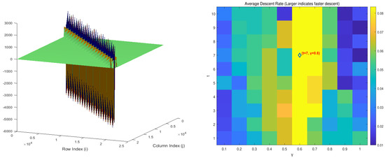
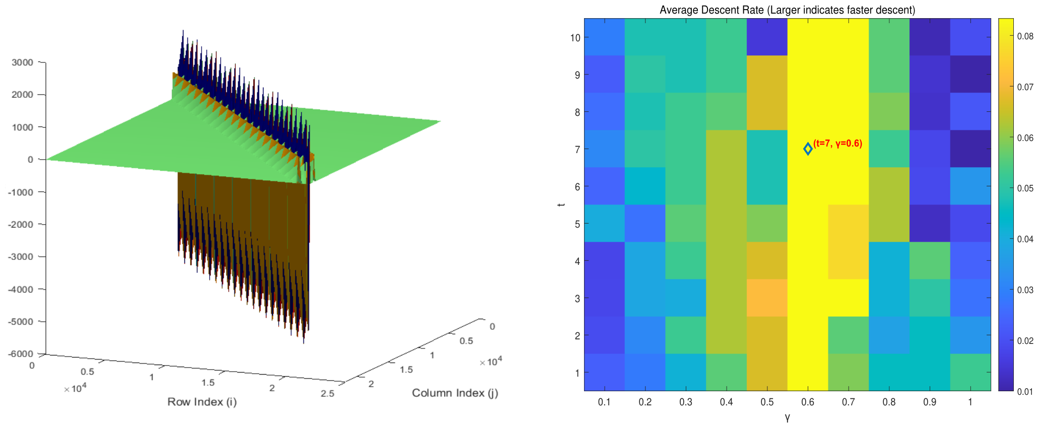
Let $N=n^3$. The derived system matrices are $A=S+L\in {\mathbb{R}}^{N\times N}$, $B=\mathtt{rand}(\mathtt{N},\mathtt{m})\in {\mathbb{R}}^{N\times m}$, and $C=B^{*}\in {\mathbb{R}}^{p\times N}$. The left subplot of Figure 1 indicates the 3D city plot of the discretized matrix A of size 21,952 ($n=28$). Here, we select $m=p=10$ to compare RADI with ARADI.

We first consider a small-scale matrix of size $n=9$ to determine relatively good parameters $(t,\gamma )$. Specifically, for various values of t (ranging from 1 to 10), we run the ARADI algorithm with $\gamma$ varying from 0.1 to 1 in steps of 0.1. For each combination of parameters, we record the residual of the equation obtained by the ARADI and the number of iterations at termination. We then define the following reduction rate

$$\begin{array}{c}\hfill \mathrm{Rate}={\displaystyle \frac{|\mathrm{Initial}\mathrm{Residual}-\mathrm{Last}\mathrm{Residual}|}{\mathrm{Iteration}\mathrm{Number}}}\end{array}$$

(40)

when the algorithm terminates.

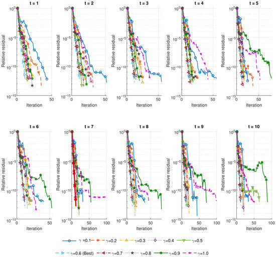
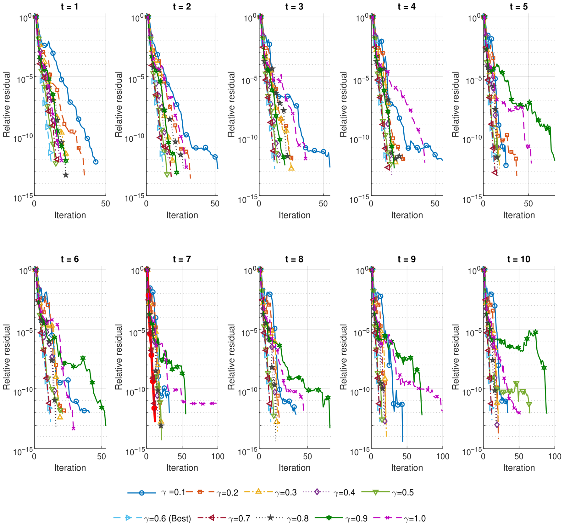
A larger value of Rate indicates faster convergence of the ARADI algorithm for the parameter pair $(t,\gamma )$. Figure 2 presents the convergence histories of the ARADI algorithm under various parameter settings, where the horizontal axis (It.) denotes the iteration number and the vertical axis represents the logarithm of the equation residual (39). It can be observed intuitively from the figure that for each value of t, certain residual curves exhibit faster convergence; these curves correspond to $\gamma$ approximately between 0.5 and 0.7. This suggests that, for this example, the ARADI algorithm is not particularly sensitive to the choice of t. The figure also highlights, for $t=7$, a thick red curve (corresponding to $\gamma =0.6$) that exhibits the fastest convergence history. The right subplot of Figure 1 shows a heat map of the Rate values for different parameter combinations, which further indicates that relatively larger Rate values occur near $\gamma =0.6$ and the maximum Rate is achieved at $(t,\gamma )=(7,0.6)$.

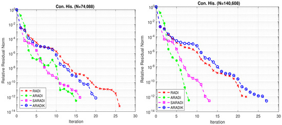
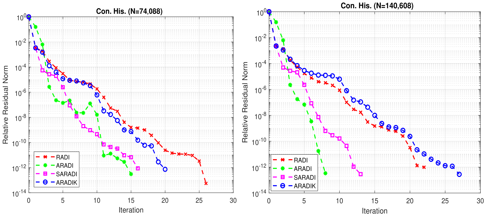
We next consider large-scale problems with the parameters fixed at $t=7$ and $\gamma =0.6$. We compare the numerical performance of all four methods (RADI, ARADI, SARADI, and ARADIK) for various nodes n, which are chosen from 34 to 52 in increments of 2, resulting in equation dimensions ranging from 39,304 to 140,608. We report in

Table 1. Numerical results of RADI vs. ARADI in Example 1.

		RADI			ARADI
$\mathbf{N}$	It.	CPU (Para.)	Res	It.	CPU (Para.)	Res
39,304	23	$73.28(0.117)$	4.94 × 10−14	9	$20.30(0.055)$	1.31 × 10−13
46,656	23	$79.22(0.222)$	8.33 × 10−13	9	$24.77(0.064)$	1.04 × 10−13
54,872	25	$114.25(0.316)$	8.58 × 10−13	9	$32.21(0.080)$	8.39 × 10−14
64,000	25	$145.94(0.363)$	8.74 × 10−14	9	$40.38(0.090)$	1.25 × 10−13
74,088	26	$194.56(0.494)$	5.58 × 10−14	15	$90.65(0.184)$	3.07 × 10−13
85,184	27	$256.04(0.492)$	8.45 × 10−13	8	$62.88(0.117)$	3.32 × 10−13
97,336	22	$302.73(0.573)$	4.54 × 10−13	8	$83.55(0.128)$	3.15 × 10−13
110,592	27	$419.69(0.780)$	2.18 × 10−14	11	$139.22(0.205)$	3.20 × 10−14
125,000	23	$444.29(0.774)$	9.99 × 10−13	8	$121.59(0.167)$	4.18 × 10−13
140,608	23	$553.94(0.970)$	9.86 × 10−13	8	$152.87(0.226)$	3.38 × 10−13

the numerical behavior of the original RADI algorithm and the best-performing algorithm, ARADI, upon termination of the iterations, where “It.” denotes the iteration counts required at termination, “CPU” indicates the computational time (“para.” in parentheses is the time for evaluation of the ADI parameters using the projected Hamiltonian see Remark 4), and “Res” represents the relative residual of the equation upon termination. The data in the table demonstrate that the ARADI algorithm outperforms RADI in all tested cases. In general, when termination occurs, ARADI requires approximately one-third to half of the iterations and the CPU time of RADI to achieve the prescribed residual accuracy. Furthermore, we present in Figure 3 the residual histories of the maximal “It.” at dimension N = 74,088 and the minimal “It.” at dimension N = 140,608. It can be observed from the left subplot that although the residual of ARADI exhibits three slight increases during the iteration process, it ultimately requires 15 iterations to reach the prescribed residual level. This shows that ARADI may trade off some accuracy for speed in some extreme scenarios. However, in our experiments, the ARADI method requires only several additional iterations to achieve, or even surpass, the accuracy of RADI, while still taking less than half the computation time of RADI. The right subplot shows that, starting from the third iteration onward, the residual of ARADI converges rapidly to the prescribed residual level, requiring only about one-third of the iterations and less than one-third of the computation time of RADI. In our numerical experiments with various dimensions, we observed that the performance of SARADI consistently lies between that of ARADI and RADI, whereas ARADIK, in many, cases performs even worse than the original RADI. This is primarily attributed to the neglect of the information in the residual matrix $R_k$ during the acceleration process.

Example 2.

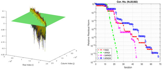
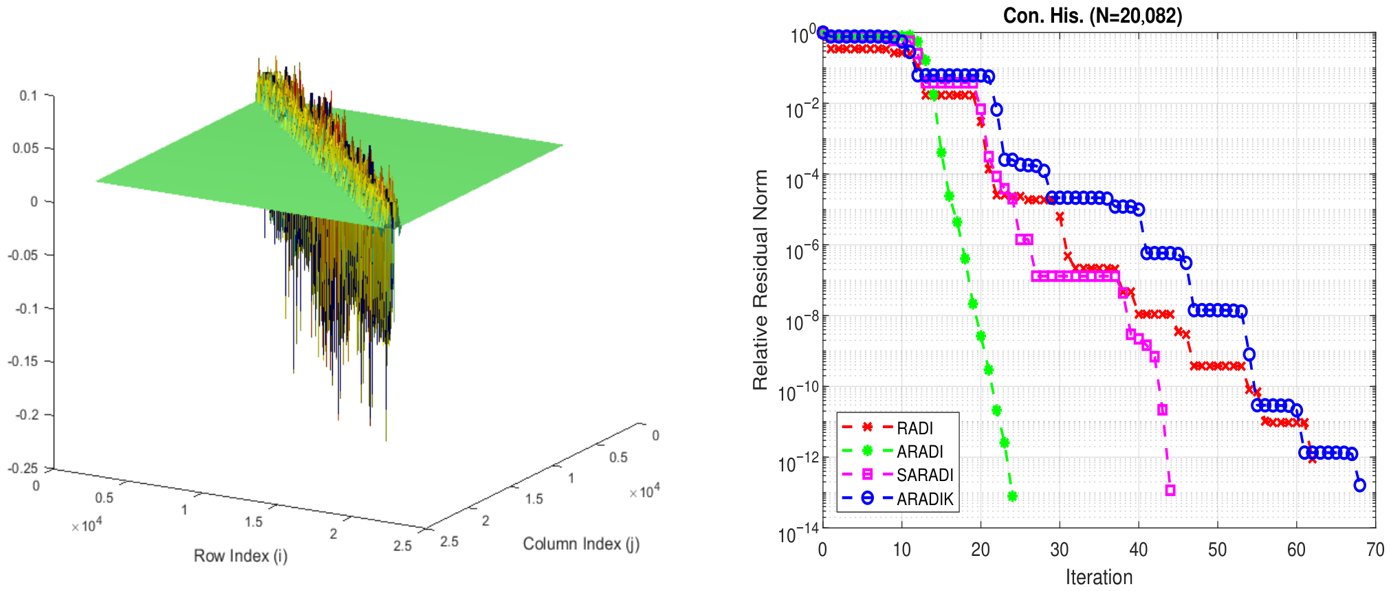
We examine the thermal convective flow control systems introduced in [30,33]. These problems are characterized by a flow domain with a prescribed velocity field, which accounts for convective transport. In the context of upwind finite element discretizations, achieving a faithful, physically meaningful solution typically necessitates a sufficiently refined mesh, as the accuracy of such schemes is known to be grid-dependent. In the representative configuration (depicted on the left side of Figure 4), a three-dimensional chip model is subjected to forced convection. The domain is discretized using tetrahedral elements of type SOLID70. Both Dirichlet boundary conditions and initial conditions are set to zero.

We consider the case where the fluid velocity is zero, implying that the discretization matrices are symmetric. The system matrices are consequently of dimensions

$$A\in {\mathbb{R}}^{\mathrm{20,082}\times \mathrm{20,082}},B\in {\mathbb{R}}^{\mathrm{20,082}\times 1},C\in {\mathbb{R}}^{5\times \mathrm{20,082}},$$

where the sparse matrices A, B, and C contain 381,276, 256, and 5 nonzero entries, respectively. Full matrix data are available from [30] and at the MOR Wiki repository (https://www.mpi-magdeburg.mpg.de/projects/mess, accessed on 30 June 2026).

We apply the ARADI algorithm with parameters $(t,\gamma )=(2,0.5)$ to solve the resulting continuous-time algebraic Riccati equation (CARE). A comparison with the RADI algorithm is also provided.

Table 2. Numerical results of various algorithms in Example 2.

N	It.	CPU (Para.)	Res	It.	CPU (Para.)	Res
		RADI			ARADI
20,800	62	$42.05(0.117)$	9.01 × 10−13	24	$15.81(0.054)$	7.90 × 10−14
		SARADI			ARADIK
20,800	44	$30.13(0.113)$	1.16 × 10−13	68	$47.72(0.145)$	1.16 × 10−13

summarizes the numerical performance of the four algorithms, where “It.”, “CPU”, and “Res” denote the number of iterations at termination, the computational time (in seconds), and the corresponding relative residual, respectively.

As can be observed from the table, the overhead for evaluating the ADI parameters is relatively negligible. RADI requires 62 iterations and approximately 42 s to achieve the prescribed residual accuracy, whereas ARADI requires only 24 iterations and about 16 s, which is slightly more than one-third of the cost incurred by RADI. SARADI takes 44 iterations to reach the prescribed residual tolerance, placing its performance between that of ARADI and RADI, while ARADIK exhibits the poorest performance among all algorithms considered. The right subplot of Figure 4 presents the residual histories of the four algorithms. It can be seen that the residual of RADI decreases in a stepwise manner. In contrast, the residual of ARADI decreases rapidly (on a logarithmic scale) after the 12th iteration and attains a smaller relative residual upon termination after 24 iterations.

Example 3.

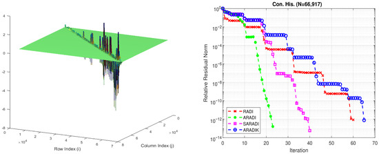
This example is derived from a numerical model that captures the electro-thermal behavior of a novel micromachined sensor device incorporating multiple thin films, with particular emphasis on the non-symmetric thermal coupling between the hotplate and the surrounding rim mediated by platinum conductor paths and the embedded heater. The model, developed exclusively for a specific sensor design, accounts for asymmetry in the thermal coupling, enabling high-fidelity simulation of the temperature distribution within the hotplate region. Spatial discretization of the governing partial differential equations is performed using the finite element method (FEM) [32] within the ANSYS 5.7 environment. Furthermore, to facilitate extraction of the underlying system matrices for subsequent model order reduction or sensitivity analysis, the Fortran subroutines native to the ANSYS 5.7 software package were modified, thereby allowing direct assembly and export of the discrete thermal system matrices as

$$\begin{array}{ccc}A\in {\mathbb{R}}^{\mathrm{66,917}\times \mathrm{66,917}},& B\in {\mathbb{R}}^{\mathrm{66,917}\times 1},& C\in {\mathbb{R}}^{28\times \mathrm{66,917}}.\end{array}$$

The 3D city plot of A is given in the left subplot of Figure 5. All matrix data are available from [30,33] and at the MOR Wiki repository (https://www.mpi-magdeburg.mpg.de/projects/mess).

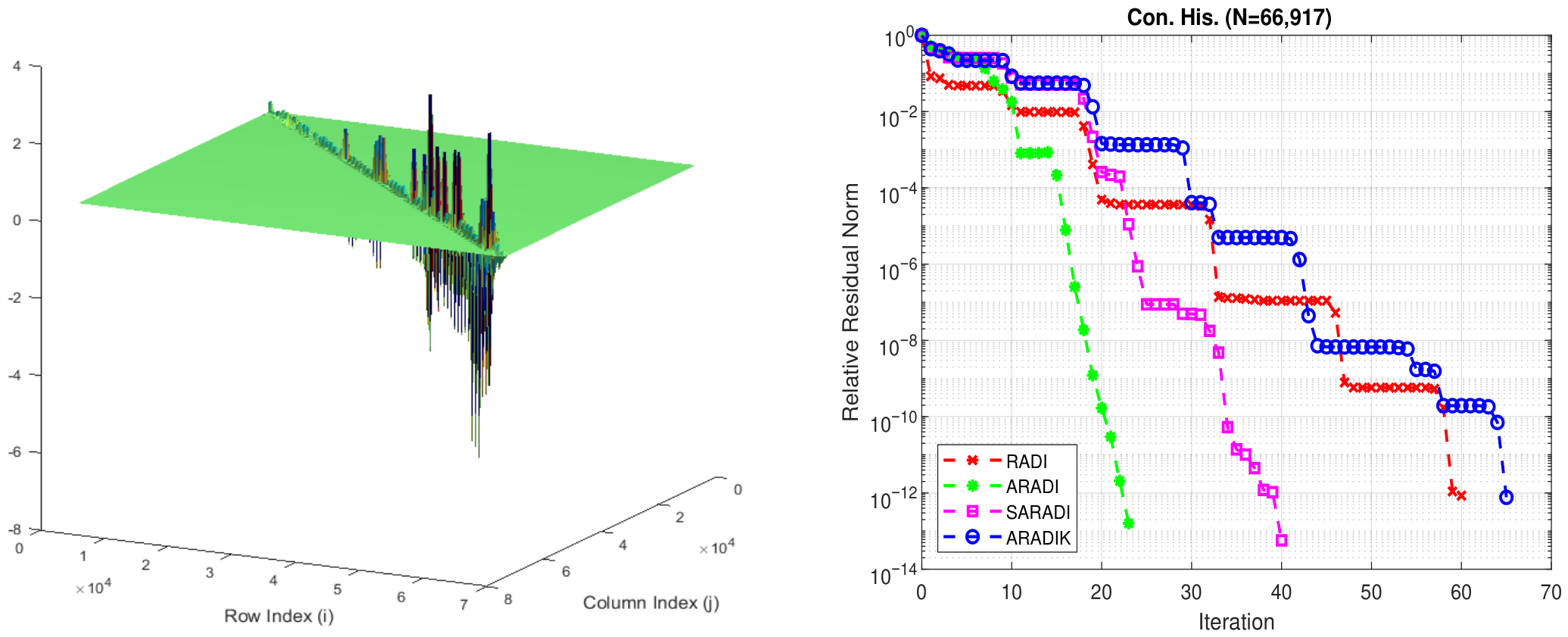
To assess the performance of the proposed ARADI algorithm for solving this example with $N=$ 66,917, we select the parameter pair $(t,\gamma )=(1,0.7)$ for ARADI and execute four algorithms. The resulting numerical results are presented in

Table 3. Numerical results of various algorithms in Example 3.

N	It.	CPU (Para.)	Res	It.	CPU (Para.)	Res
		RADI			ARADI
66,917	60	$98.11(3.895)$	8.52 × 10−13	23	$35.74(1.562)$	1.60 × 10−13
		SARADI			ARADIK
66,917	39	$65.92(2.66)$	9.17 × 10−14	65	$144.49(4.234)$	7.70 × 10−13

for comparison.

It can be observed that ARADI achieves the residual level of 10⁻¹³ within only 23 iterations, with a total CPU time of approximately 35 s. In contrast, RADI requires nearly three times as many iterations (60) and CPU time (98 s) as ARADI. Again, SARADI takes 39 iterations to reach the residual level below 10⁻¹², performing intermediately between ARADI and RADI. In contrast, ARADIK demands the highest number of iterations and the longest CPU time upon termination, thus delivering the poorest performance among all algorithms. Similarly, we plot the residual histories of the four algorithms in the right subplot of Figure 5. From the figure, it can be seen that the residual reduction of RADI decreases slowly in a stepwise manner. For ARADI, apart from a slight stagnation from iterations 11 to 14, the residual drops very rapidly as the iteration count rises, ultimately achieving a smaller equation residual upon termination after 23 iterations than that obtained by RADI at its termination.

Example 4.

The optimal cooling process of steel profiles, when governed by automated control systems, leads to a semi-discretized heat transfer model [30]. The dimensionality of the resulting dynamical system is determined by the degree of refinement of the computational mesh. Spatial discretization is carried out using linear Lagrange elements, implemented through the ALBERTA-1.2 finite element toolbox [32].

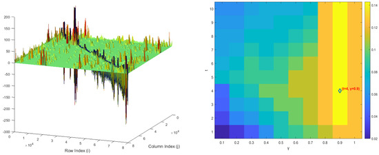
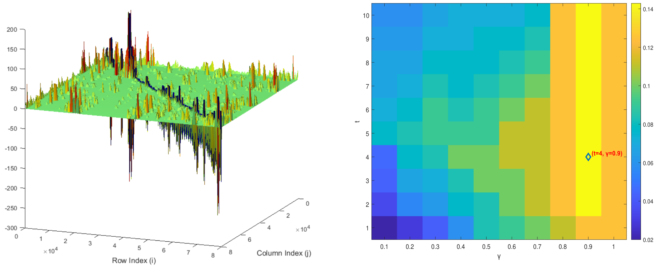
The derived system matrices $A_0\in {\mathbb{R}}^{N\times N}$, $B\in {\mathbb{R}}^{N\times m}$, and $C\in {\mathbb{R}}^{p\times N}$ are all sparse and can be obtained at the MOR Wiki repository (https://www.mpi-magdeburg.mpg.de/projects/mess). To ensure the convergence of the four algorithms, a spectral shift is applied to $A_0$; specifically, we set $A=A_0-\sigma I_N$, where $\sigma$ is taken as 0.4 times the magnitude of the largest real-part eigenvalue of $A_0$. This shifted matrix A is used uniformly across all algorithms, and the shift does not alter the original low-rank structure. We consider N = 20,209 and 79,841, and the 3D city plot of size 79,841 is given on the left of Figure 6. To obtain relatively satisfactory parameters, we ran ARADI on a medium-scale equation of 5129 using different values of t and $\gamma$. The right subplot of Figure 6 presents a heatmap of the reduction rate, indicating that the Rate defined in (40) attains its maximum at $(t,\gamma )=(4,0.9)$, which is adopted for large-scale problems of dimension $N=$ 20,209 and 79,841.

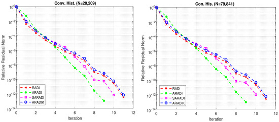
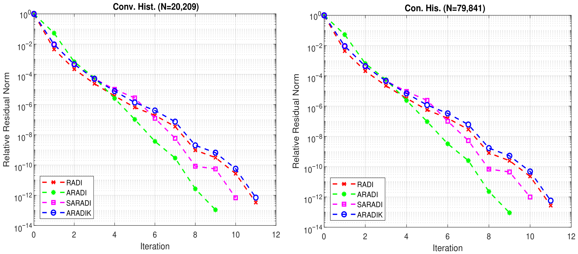
The obtained numerical results are summarized in

Table 4. Numerical results of various algorithms in Example 4.

N	It.	CPU (Para.)	Res	It.	CPU (Para.)	Res
		RADI			ARADI
20,209	11	$3.40(0.290)$	3.33 × 10−13	9	$1.46(0.020)$	1.09 × 10−13
79,841	11	$17.32(0.138)$	2.72 × 10−13	9	$7.22(0.111)$	9.03 × 10−14
		SARADI			ARADIK
20,209	10	$2.41(0.270)$	6.82 × 10−13	11	$2.81(0.024)$	7.00 × 10−13
79,841	10	$12.63(0.129)$	9.90 × 10−13	11	$14.45(0.128)$	5.73 × 10−13

. It can be observed from the table that, for different dimensions N, RADI requires 11 iterations to achieve the prescribed residual accuracy, whereas ARADI needs only 9 iterations. The CPU time column indicates that, for each N, the elapsed time for RADI upon termination is more than twice that of ARADI. Consistent with previous examples, SARADI reaches a residual level of 10⁻¹³ in 10 iterations, placing its performance between ARADI and RADI. In comparison, ARADIK requires the same number of iterations as RADI but incurs less CPU time. Nevertheless, it still converges more slowly than ARADI and SARADI. Furthermore, we plot the residual histories of the four algorithms in Figure 7. The figure shows that, after 4 iterations, ARADI maintains a lower residual level than RADI and ultimately attains a smaller equation residual upon termination.

5. Conclusions

We have developed an accelerated RADI iteration for large-scale CAREs. Unlike approaches that view RADI solely as a function of the feedback gain matrix and accelerate only the feedback sequence, our approach treats the combined feedback gain and residual matrices as a unified iterate and interprets the ARADI iteration as a nonlinear mapping, thereby constructing an effective RADI acceleration strategy. Numerical results on practical engineering problems indicate that, with appropriate parameter choices, both the proposed safeguarded ARADI (SARADI) algorithm and its unsafeguarded special case, ARADI, attain the prescribed residual tolerance using substantially fewer iterations and reduced computational cost. It is worth noting that the number of residual steps t used for acceleration and the damping factor $\gamma$ are critical factors in the success of the ARADI algorithm. For equations of fixed dimension, our computational experience indicates that when the initial residual does not exceed $O(1)$ and exhibits sufficiently fast decay in the early iterations, a relatively large choice of the parameter t may be effective. In contrast, slow residual reduction during the initial stage calls for a relatively small t. As for the damping factor, we find that setting it to approximately 0.5 makes the acceleration effect relatively conspicuous. Existing experimental results indicate that the above strategy is at least empirically successful.

One point that merits emphasis is that, although the proposed algorithm works well numerically under the aforementioned parameter selection strategy, developing an adaptive strategy for selecting these parameters in practical engineering applications remains an important direction for future research, as it would significantly enhance the generality and robustness of the method.

References

- Lancaster, P.; Rodman, L. Algebraic Riccati Equations; Clarendon Press: Oxford, UK, 1995. [Google Scholar]
- Benner, P. Editorial of special issue on “Large-Scale Matrix Equations of Special Type”. Numer. Lin. Alg. Appl. 2008, 15, 747–754. [Google Scholar]
- Benner, P.; Fassbender, H. On the numerical solution of large-scale sparse discrete-time Riccati equations. Adv. Comp. Math. 2011, 35, 119–147. [Google Scholar]
- Benner, P.; Li, J.-R.; Penzl, T. Numerical solution of large Lyapunov equations, Riccati equations and linear-quadratic control problems. Numer. Lin. Alg. Appl. 2008, 15, 755–777. [Google Scholar] [CrossRef] [Scilit]
- Chu, E.K.-W.; Fan, H.-Y.; Lin, W.-W. A structure-preserving doubling algorithm for continuous-time algebraic Riccati equations. Linear Algebra Its Appl. 2005, 396, 55–80. [Google Scholar] [CrossRef] [Scilit]
- Chu, E.K.-W.; Fan, H.-Y.; Lin, W.-W.; Wang, C.-S. A structure-preserving doubling algorithm for periodic discrete-time algebraic Riccati equations. Int. J. Control 2004, 77, 767–788. [Google Scholar] [CrossRef] [Scilit]
- Yu, B.; Fan, H.-Y.; Chu, E.K.-W. Large-scale algebraic Riccati equations with high-rank constant terms. J. Comput. Appl. Math. 2019, 361, 130–143. [Google Scholar]
- Li, T.-X.; Chu, E.K.-W.; Lin, W.-W.; Weng, P.C.-Y. Solving large-scale continuous-time algebraic Riccati equations by doubling. J. Comput. Appl. Math. 2013, 237, 373–383. [Google Scholar] [CrossRef] [Scilit]
- Heyouni, M.; Jbilou, K. An extended block Arnoldi algorithm for large-scale solutions of the continuous-time algebraic Riccati equations. Electron. Trans. Numer. Anal. 2009, 33, 53–62. [Google Scholar]
- Jbilou, K. Block Krylov subspace methods for large continuous-time algebraic Riccati equations. Numer. Algorithms 2003, 34, 339–353. [Google Scholar]
- Jbilou, K. An Arnoldi based algorithm for large algebraic Riccati equations. Appl. Math. Lett. 2006, 19, 437–444. [Google Scholar] [CrossRef] [Scilit]
- Druskin, V.; Simoncini, V.; Zaslavsky, M. Adaptive tangential interpolation in rational Krylov subspaces for MIMO dynamical systems. SIAM J. Matrix Anal. Appl. 2014, 35, 476–498. [Google Scholar] [CrossRef] [Scilit]
- Druskin, V.; Knizhnerman, L.A. Extended Krylov subspaces: Approximation of the matrix square root and related functions. SIAM J. Matrix Anal. Appl. 1998, 19, 755–771. [Google Scholar] [CrossRef] [Scilit]
- Druskin, V.; Knizhnerman, L.A.; Simoncini, V. Analysis of the rational Krylov subspace and ADI methods for solving the Lyapunov equation. SIAM J. Numer. Anal. 2011, 49, 1875–1898. [Google Scholar] [CrossRef] [Scilit]
- Simoncini, V. Analysis of the rational Krylov subspace projection method for large-scale algebraic Riccati equations. SIAM J. Matrix Anal. Appl. 2016, 37, 1655–1674. [Google Scholar] [CrossRef] [Scilit]
- Stykel, T.; Simoncini, V. Krylov subspace methods for projected Lyapunov equations. Appl. Numer. Math. 2012, 62, 35–50. [Google Scholar] [CrossRef] [Scilit]
- Jin, J.C.; Dong, N.; Cai, R.Z. A quick iterative algorithm for quadratic equations in an overdamped system. J. Hunan Univ. Tech. 2018, 32, 1–5. [Google Scholar] [CrossRef]
- Meng, Z.; Dong, N.; Yu, B.; Liao, S. A numerical iterative algorithm for coupled Riccati equations. J. Hunan Univ. Tech. 2020, 34, 14–18. [Google Scholar] [CrossRef]
- Benner, P.; Bujanović, Z.; Kürschner, P.; Saak, J. A numerical comparison of different solvers for large-scale, continuous-time algebraic Riccati equations and LQR problems. SIAM J. Sci. Comput. 2020, 42, A957–A996. [Google Scholar] [CrossRef] [Scilit]
- Benner, P.; Bujanović, Z.; Kürschner, P.; Saak, J. RADI: A low-rank ADI-type algorithm for large scale algebraic Riccati equations. Numer. Math. 2018, 138, 301–330. [Google Scholar] [PubMed]
- Anderson, D.G. Iterative procedures for nonlinear integral equations. J. Assoc. Comput. Mach. 1965, 12, 547–560. [Google Scholar] [CrossRef] [Scilit]
- Evans, C.; Pollock, S.; Rebholz, L.; Xiao, M. A proof that Anderson acceleration improves the convergence rate in linearly converging fixed point methods (but not in those converging quadratically). SIAM J. Numer. Anal. 2020, 58, 788–810. [Google Scholar] [CrossRef] [Scilit]
- Rebholz, L.; Xiao, M. The effect of Anderson acceleration on superlinear and sublinear convergence. J. Sci. Comput. 2023, 96, 34. [Google Scholar] [CrossRef] [Scilit]
- Pollock, S.; Rebholz, L. Anderson acceleration for contractive and noncontractive operators. IMA J. Numer. Anal. 2021, 41, 2841–2872. [Google Scholar] [CrossRef] [Scilit]
- Higham, N.J. Functions of Matrices: Theory and Computation; SIAM: Philadelphia, PA, USA, 2008. [Google Scholar]
- Wong, N.; Balakrishnan, V. Quadratic alternating direction implicit iteration for the fast solution of algebraic Riccati equations. In Proceedings of International Symposium on Intelligent Signal Processing and Communication Systems; IEEE: New York, NY, USA, 2005; pp. 373–376. [Google Scholar]
- Wong, N.; Balakrishnan, V. Fast positive-real balanced truncation via quadratic alternating direction implicit iteration. IEEE Trans. Comput.-Aided Des. Integr. Circuits Syst. 2007, 26, 1725–1731. [Google Scholar] [CrossRef] [Scilit]
- Dieudonné, J. Foundations of Modern Analysis; Academic Press: New York, NY, USA, 1960. [Google Scholar]
- Benner, P.; Bujanović, Z. On the solution of large-scale algebraic Riccati equations by using low dimensional invariant subspaces. Linear Algebra Its Appl. 2016, 488, 430–459. [Google Scholar] [CrossRef] [Scilit]
- Korvink, G.; Rudnyi, B. Oberwolfach Benchmark Collection. In Dimension Reduction of Large-Scale Systems; Benner, P., Sorensen, D.C., Mehrmann, V., Eds.; Lecture Notes in Computational Science and Engineering; Springer: Berlin/Heidelberg, Germany, 2005; p. 45. [Google Scholar]
- Lang, N. Numerical Methods for Large-Scale Linear Time-Varying Control Systems and Related Differential Matrix Equations; Logos-Verlag: Berlin, Germany, 2018. [Google Scholar]
- Schmidt, A.; Siebert, K. Design of Adaptive Finite Element Software—The Finite Element Toolbox ALBERTA; Lecture Notes in Computational Science and Engineering; Springer: Berlin/Heidelberg, Germany, 2005; Volume 42. [Google Scholar]
- Chahlaoui, Y.; Van Dooren, P. Benchmark examples for model reduction of linear time-invariant dynamical systems, dimension reduction of large-scale systems. In Dimension Reduction of Large-Scale Systems; Springer: Berlin/Heidelberg, Germany, 2005; Volume 45, pp. 379–392. [Google Scholar]
Disclaimer/Publisher’s Note: The statements, opinions and data contained in all publications are solely those of the individual author(s) and contributor(s) and not of MDPI and/or the editor(s). MDPI and/or the editor(s) disclaim responsibility for any injury to people or property resulting from any ideas, methods, instructions or products referred to in the content. |
© 2026 by the authors. Licensee MDPI, Basel, Switzerland. This article is an open access article distributed under the terms and conditions of the Creative Commons Attribution (CC BY) license.