Feature Stability as a Trust Layer for Feature Selection: Resampling-Based Recurrence Profiles Beyond Predictive Performance

Abstract

Feature selection in high-dimensional studies is conventionally evaluated by the predictive performance of the features it returns, but predictive performance does not indicate whether the same subset would be selected again under a reasonable perturbation of the data. We propose a feature-stability profile, reported as a diagnostic layer beside predictive performance rather than in place of it. The profile is assembled from established quantities: per-feature selection frequency across repeated stratified resamples, a chance-corrected stability summary, recurrent sets reported across a sweep of descriptive cutoffs, a random-selection baseline, and the held-out predictive performance recorded on the same resamples. We examine it in two settings. In a controlled synthetic study, the informative support is planted by construction, so recovery can be measured directly; in an illustrative application across high-dimensional binary datasets, no such support exists, and a broader exploratory roster is reported as supporting results. Under planted support, predictive performance, subset stability, and support recovery can diverge rather than decline together: at an intermediate signal level, performance can remain relatively preserved while exact recovery falls, and some low exact overlap reflects substitution among redundant alternatives. On real data, recurrent features are treated as recurrent candidates, not recovered or validated features; selectors reaching near-equal area under the receiver operating characteristic curve (AUC) can differ about twofold in chance-corrected recurrence. The contribution is diagnostic and integrative, not a new selector, a new metric, a benchmark ranking, or an error-controlled procedure, making the reliability of a selected feature set visible rather than assumed.

1. Introduction

Feature selection is a standard component of modern high-dimensional analysis, and its success is conventionally judged by the predictive performance of the features it returns: a subset that supports accurate downstream classification is often treated as successful [1,2]. Yet predictive performance and the identity of the selected subset are distinct properties, and accuracy certifies little about the stability of the selection. A selector can attain high held-out performance while returning a materially different subset under modest perturbations of the data, so that the subset offered to a practitioner as an object of interpretation and explanation is not, by accuracy alone, shown to be reproducible [3]. This gap matters because the selected subset is frequently read as a substantive, parsimonious account of which measured quantities carry information, an inferential use that performance metrics were never designed to underwrite [4]. Treating predictive performance as the sole criterion therefore leaves a reliability dimension of feature selection unexamined. The stability of a selected subset under reasonable variation in the data is thus a distinct concern, and one with a long-standing place in the feature-selection literature.

That stability is a recognized concern, rather than a new one, is evident at two levels. Methodologically, the view that empirical conclusions should remain stable under reasonable perturbations of the data, model, and analytic choices has become a widely endorsed standard for trustworthy data analysis [5]. Within feature selection specifically, the sensitivity of selected subsets to small changes in the training sample was documented early and has been revisited repeatedly, particularly in high-dimensional regimes, where correlated variables and limited sample sizes make the chosen subset unusually dependent on the data at hand [3]. In response, a sustained line of work has sought to characterize and improve this stability, including resampling and ensemble strategies that aggregate selections over perturbed samples so that consistently recurring features can be distinguished from incidental ones [6]. The present work is situated firmly within this tradition: we treat the reproducibility of a selected subset as an established property worth examining, not as a novel proposal. Examining it, however, presupposes a means of measuring it, and how selection stability should itself be quantified is a question this literature has had to confront directly.

A substantial methodological literature has consequently developed around the measurement of selection stability. The earliest and most transparent measures quantify the agreement between subsets selected on perturbed samples directly, using raw set-overlap coefficients such as the Jaccard, Tanimoto, Dice–Sørensen, or Ochiai indices to express how extensively two selected subsets share features [3,7,8,9,10]. While appealingly simple, such measures conflate genuine reproducibility with the overlap expected by chance, which varies with both the size of the selected subset and the dimensionality of the candidate pool; the same nominal overlap may therefore signal strong agreement in one regime and near-randomness in another. Subsequent work addressed this by introducing chance-corrected indices that calibrate observed overlap against its expectation under random selection, with the Kuncheva consistency index being the most widely used [11]. More recent contributions have reframed stability measurement axiomatically, articulating the formal properties a principled index ought to possess (correction for chance, boundedness independent of dimensionality, and strict monotonicity) and proposing estimators that satisfy them while admitting confidence intervals and significance tests [10], now consolidated in shared tooling [12]. The result is a mature apparatus for quantifying how much a selection changes under perturbation; however, it speaks far less to why those changes arise, or to how they should be interpreted.

One reason selected subsets vary deserves particular emphasis: instability is not invariably a symptom of algorithmic failure. High-dimensional data routinely contain correlated and redundant predictors, so that a single underlying source of signal is carried by several near-equivalent features rather than by one [13]. Under modest perturbations of the sample, a selector may then exchange one member of such a correlated group for another across resamples, producing a visibly different reported subset even as the information that subset encodes (and the downstream predictive performance it supports) remains largely preserved. This substitution behaviour is well documented for sparse selectors, where an L1 penalty typically retains a single representative of a correlated block and discards its peers, but the identity of the survivor is itself sample-dependent; analogous dilution of importance across correlated features arises in embedded and ensemble methods [14]. Low subset overlap may therefore reflect interchange among redundant proxies rather than a failure to identify the relevant signal. It need not, however: the same low overlap can equally arise from genuine instability, and from a set-overlap comparison alone the two are indistinguishable [13]. Separating benign substitution from genuine inconsistency thus calls for attention not merely to whether features recur, but to how frequently each recurs across many perturbed selections.

Attending to how often a feature recurs, rather than merely whether it appears in one selection, is the organizing principle of resampling-based feature selection. Instead of inspecting a single subset, these approaches perturb the data many times (through subsampling or the bootstrap), refit the selector on each perturbed sample, and summarize each feature by the fraction of fits in which it is selected, a quantity variously termed its selection frequency or estimated selection probability [6]. Ensemble feature-selection methods rest on the same foundation, combining selections across perturbed fits so that features chosen consistently are favoured over those selected only intermittently [15]. The appeal of this representation is that it supplants a binary membership verdict with a graded one: every candidate feature is located on a recurrence spectrum running from almost never selected to almost always selected, and a feature’s position on that spectrum, rather than its presence in any one subset, becomes the object of interest [16]. Methodological refinements of the resampling protocol, including complementary-pair subsampling, have further improved the reliability of these frequency estimates [17]. Selection frequency is, in short, a well-established backbone for describing recurrence under perturbation. Acting on it, however, reintroduces a difficulty: deciding how frequently a feature must recur before it is deemed reliably selected is itself a non-trivial choice.

This difficulty is intrinsic to the frequency representation. To declare a feature reliably selected, one must place a cutoff on its selection frequency, and recurrence cutoffs such as 0.6, 0.8, or 0.9 have been adopted in prior practice for this purpose [6]. Such thresholding is genuinely useful: it distils a continuous recurrence profile into a discrete recurrent set that can be reported and compared across selectors. Its limitation is that the cutoff is partly conventional rather than dictated by the data, and the apparent size and composition of the recurrent set can change materially as the cutoff is moved across its plausible range: a feature recurring in seventy percent of resamples belongs to the set under a 0.6 cutoff but not under a 0.8 one, though nothing about the underlying selection has changed. Collapsing stability onto the set induced by a single fixed threshold therefore risks attaching undue weight to a conventional choice. Two established practices guard against this: reporting the recurrent set across a span of cutoffs rather than at one value, and retaining the chance-corrected [11] and threshold-free, axiomatically grounded [10] summaries that characterize stability without reference to any cutoff. Taken together, a frequency profile and these cutoff-independent summaries describe a selection’s stability more fully than any single recurrent set, suggesting that stability is better reported in profile, alongside predictive performance, than reduced to one figure.

What joint reporting of this kind would reveal has not yet been examined systematically. Stability is most often reported in isolation, or compressed into a single summary, rather than set beside predictive performance in a way that reveals when the two diverge; and on real data several further properties of a selection (whether it recovers the features that genuinely matter) cannot be assessed at all, since they presuppose a ground truth that real data does not supply. In this work we present a diagnostic stability profile, reported alongside predictive performance, that assembles established components (per-feature selection frequency, a recurrent set reported across a range of cutoffs, and the chance-corrected and threshold-free summaries already standard in the literature) into a single descriptive characterization of a selector’s output. The contribution is integrative and diagnostic: by computing established components together and reporting them beside performance, the profile makes a selection’s reliability visible. Through a controlled synthetic proof-of-concept, in which the informative features are planted and hence known, we demonstrate that predictive performance, subset stability, exact support recovery, proxy-aware recovery, behaviour against a signal-free null, and the instance-dependence of recovery can diverge rather than vary in concert. We then report an illustrative real-data application, on high-dimensional datasets for which no ground truth exists, in which predictive performance and stability are likewise seen to come apart and the profile serves a purely descriptive, diagnostic role. The practical novelty of the proposed profile is the operational integration of established stability quantities into a diagnostic trust layer for feature selection. By aligning per-feature recurrence frequencies, recurrent-set thresholds, chance-corrected stability, random-selection baselines, synthetic recovery when planted support is known, and held-out predictive performance in a single side-by-side view, the profile makes visible a reliability question that predictive performance alone cannot answer: whether the features selected by a procedure recur consistently under data perturbation. The contribution accordingly complements existing feature selectors, stability indices, and stability-selection procedures rather than replacing them; it introduces neither a new selector, nor a new scalar stability index, nor an error-controlled selection guarantee.

Section 2 positions the work relative to existing stability measures, stability-selection methods, and performance-focused evaluation; Section 3 formalizes the profiling protocol and its claim boundaries; Section 4 reports the synthetic controlled study and the real-data illustrative application; and Section 5 discusses interpretation, limitations, and the diagnostic use of the profile.

2. Related Work

2.1. Evaluating Feature Selection Beyond Predictive Performance

The evaluation of feature selection has, for the most part, been organized around predictive performance. Broad surveys of the field present feature selection chiefly as a means to accurate, parsimonious models and catalogue methods by the predictive gains they afford [1,2,18]; dedicated benchmarking studies extend this view, comparing selection procedures across heterogeneous datasets and learners according to the downstream accuracy they enable [19,20,21]. Alongside these comparative efforts, a careful methodological literature has scrutinized how predictive performance ought to be estimated. It has shown that evaluation pipelines that apply feature selection outside the cross-validation loop, or that conflate model selection with performance assessment, produce systematically optimistic estimates [22,23], a bias that continues to surface in applied high-dimensional analyses despite being well documented [24]. A further strand has examined the choice of performance measure itself, observing that accuracy and threshold-dependent summaries can be misleading under class imbalance and that chance-corrected or precision–recall-based metrics often convey more faithful comparisons [25,26]. Taken together, this work has substantially advanced the rigour with which the predictive quality of a selected subset is measured. Its concern, however, remains the performance the features support rather than the reproducibility of the selection that produced them: whether a procedure would return a comparable set of features on comparable data is a question this evaluation machinery is not designed to answer, yet it is precisely the question on which interpreting the selected subset depends. The rich evaluation literature on predictive quality should accordingly be complemented by a separate literature concerned with measuring the stability of feature selection itself.

2.2. Measuring Selection Stability: Set-Overlap, Chance-Corrected, and Axiomatic Indices

The reliability dimension that performance evaluation leaves unaddressed is the subject of a substantial measurement literature, which formalizes stability as the robustness of a selector’s feature preferences to perturbations of the training data [3]. Quantifying this robustness begins with comparing the subsets a selector returns on different perturbed samples, and the earliest measures express such agreement directly as set overlap, for instance, through the Jaccard coefficient. The difficulty is not that overlap is uninformative but that it is hard to interpret on its own: the agreement two unrelated selections would exhibit by chance depends on the size of the selected subset and on the dimensionality of the candidate pool, so a given overlap value carries different meaning across different problems. Chance-corrected indices resolve this by calibrating observed overlap against its expectation under random selection, producing a quantity that can be compared meaningfully across regimes [11]. A later, axiomatic perspective makes the desiderata explicit (among them correction for chance and behaviour that does not drift with dimensionality) and accompanies them with estimators and sampling distributions, so that selection stability acquires the status of an estimable population quantity reportable with an associated uncertainty rather than as a single figure [10]. Complementary work extends stability assessment beyond binary set membership, for example, by weighting features according to their importance [16], and studies stability empirically as a property of selectors in high-dimensional biomedical settings [27,28]. These measures are mature, well-motivated, and now consolidated in openly available software [12]. We build on them directly: rather than proposing a new index, we reuse these established chance-corrected and axiomatically grounded summaries and report them alongside other descriptive components of a selector’s output. These measurement tools quantify variation in selected subsets, while resampling-based methods provide the operational mechanism by which selection recurrence is estimated.

2.3. Resampling-Based Selection: Stability Selection, Error Control, Ensemble Aggregation, and the Cutoff Question

Assessing how often a feature recurs rests on a resampling mechanism: the selector is refit on many perturbed realizations of the data (generated by subsampling or by the bootstrap) and each feature is characterized by the frequency, or estimated selection probability, with which it is chosen across those fits. This device was given a precise inferential reading by stability selection, which paired the estimated selection probability with a finite-sample result: under stated assumptions, retaining only features whose selection probability exceeds a chosen threshold bounds the expected number of false selections [6]. Complementary-pair stability selection subsequently strengthened this line, deriving tighter error bounds under weaker assumptions through a structured subsampling scheme [17]. Ensemble feature selection draws on the same resampling principle but with a different emphasis, combining selections across perturbed fits chiefly to reduce variance and produce a more robust aggregate selection rather than to certify a formal error rate [15,29]. Turning the resulting continuous frequency profile into a discrete set of reliably selected features nonetheless requires a selection-probability cutoff. The conventional choices (commonly between 0.6 and 0.9, originating in the stability-selection literature) are useful but partly conventional: which features fall inside the recurrent set changes as the cutoff is moved, a sensitivity that reporting the set across a range of cutoffs makes explicit, while the threshold-free indices of the preceding subsection continue to summarize stability without committing to any one value. It bears emphasis that our work reuses this resampling mechanism and the selection-frequency representation in a purely descriptive capacity. We neither adopt stability selection as a selection method nor inherit the false-discovery or per-family error-control guarantees it and its refinements were designed to deliver; those guarantees follow from specific penalties, subsampling schemes, and assumptions that a descriptive profile over an unmodified selector does not invoke. Even when recurrence is estimated carefully, correlated and redundant predictors can make feature identities interchangeable, so stability must be interpreted in light of substitution effects.

2.4. Redundancy, Correlated Predictors, and Redundancy-Aware Selection

The interchangeability of feature identities under perturbation, noted at the close of the previous subsection, has a well-characterized origin in the structure of high-dimensional data. When predictors are correlated or redundant, the signal a selector depends on is distributed across several near-equivalent variables rather than localized in one, and sparse selectors in particular tend to retain a single representative of a correlated group while discarding its peers [30]. Because the surviving representative is itself determined by the particular sample, the reported subset can shift markedly from one resample to the next even as the information that subset conveys remains essentially intact, a phenomenon analysed in detail for feature ranking and selection in the presence of correlated predictors [13]. Interpreted accordingly, low subset overlap does not by itself imply that a selector has failed to recover the relevant signal; it may instead reflect substitution among proxies for a shared underlying source. A distinct line of work confronts redundancy by intervention rather than by diagnosis. Penalties that induce correlated variables to enter or leave the model together reduce the arbitrariness of selecting one member of a correlated block [14], and relevance–redundancy criteria select features by explicitly balancing their relevance against their redundancy with features already chosen [31,32]. Such methods alter the selection procedure itself to manage correlated and redundant predictors. The diagnostic profile developed here is complementary to, and not in competition with, these approaches: it does not modify the selector or remove redundancy, but it can help reveal whether observed instability may arise from substitution among correlated proxies, from weak signal, or from more general unreliability, a distinction that should be interpreted in light of the data-generating setting rather than asserted as a definitive judgement. The interpretation of stability is therefore inseparable from the data-generating setting, and this makes controlled synthetic designs and explicit ground-truth limits important.

2.5. Dataset Hardness, Ground-Truth Limits, and Synthetic Controls

A final consideration concerns where each kind of claim can legitimately be made. Whether a selector recovers the features that genuinely carry signal can be evaluated directly only when those features are known in advance. Controlled synthetic settings make this possible: because the informative variables are planted by construction, a selected subset can be compared against a known support, which renders such designs well suited to internal-validity checks of whether a procedure recovers, or fails to recover, the relevant features. Real datasets seldom permit comparisons of this kind. Beyond engineered problems, the relevance of a measured quantity is generally unobserved, so analysis on real data cannot establish support recovery and must remain descriptive in character: it can report which features are recurrently selected and how stable a selection is across perturbations, but it cannot certify those recurrent candidates as the correct or relevant ones. A complementary literature clarifies why neither stability nor recovery should be presumed uniform across problems. Work on data complexity and classification difficulty demonstrates that datasets differ systematically in their intrinsic hardness [33,34], with openly available tooling for quantifying these properties [35], and dataset difficulty has been related directly to feature-selection behaviour and benchmarking [36]; in high-dimensional regimes, moreover, the apparent quality and variability of a selection can be substantially distorted unless the evaluation procedure is constructed with care [22]. In combination, these observations recommend a clear separation between recovery-oriented claims, which presuppose a known ground truth, and descriptive stability claims, which do not, recognizing that a controlled study and a real-data application support internal validity and external plausibility, respectively, and that neither alone establishes generality. This distinction motivates the empirical design that follows: a controlled synthetic study for recovery-oriented claims, and a real-data application for descriptive stability profiling.

3. Materials and Methods

For readability, Abbreviations and Notation section summarizes the abbreviations and notation used throughout the stability-profiling protocol.

3.1. Overview of the Stability-Profiling Pipeline

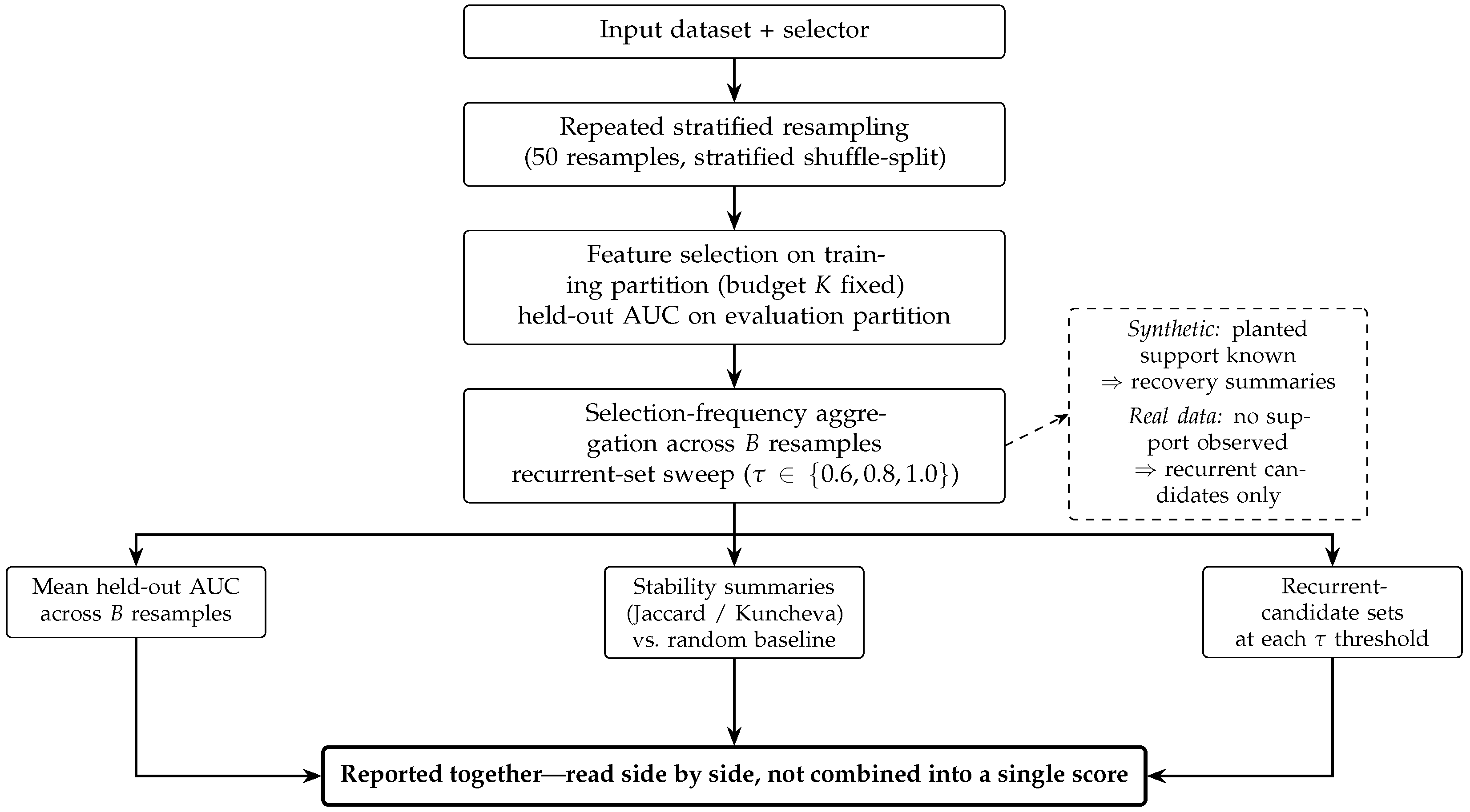
The two empirical studies reported below are instances of a single stability-profiling pipeline, applied throughout to an unmodified feature selector rather than to a new selection procedure of our own. The pipeline takes an input dataset and produces many perturbed realizations of the training data through repeated stratified resampling; on each realization the selector is refit, with the number of features it returns held fixed at a chosen budget. No part of the selector or its selection rule is altered: the procedure characterizes the selector as it is ordinarily applied. From the repeated fits we compute, for every candidate feature, the proportion of resamples in which it is selected, yielding a per-feature selection-frequency profile of the kind used in resampling-based selection [6]. A frequency cutoff turns this continuous profile into a discrete recurrent set; rather than commit to one cutoff, the procedure reports the recurrent set across a sweep of cutoff values, so that the dependence of the set on the chosen threshold is made visible. In parallel, we compute established chance-corrected and threshold-free stability summaries [10,11], evaluated against a random-selection baseline, and we record the held-out predictive performance attained on each fit, so that predictive performance is reported alongside stability rather than as a substitute for it. What may be inferred from the profile depends on the setting in which it is computed. When the informative features are planted by construction and the support is therefore known, we additionally compute recovery summaries that compare the selected features against that known support. When feature relevance is unobserved, no such comparison is possible, and the analysis is restricted to descriptive characterization of recurrent candidates against the random baseline, without reference to a ground truth. Figure 1 summarizes this workflow and emphasizes that the profile components are reported together rather than collapsed into a single score. Later subsections specify the resampling protocol, the stability summaries, the synthetic controlled setting, the real-data application, the claim boundaries, and the implementation details.

3.2. Resampling and Evaluation Protocol

The perturbation mechanism is repeated stratified resampling, implemented as a stratified shuffle-split that preserves the class proportions of the full sample within each draw. We generate 50 resamples, each holding out a fraction of 0.2 of the observations as an evaluation partition and retaining the remainder as a training partition, and we fix the random seed so that the same family of partitions is reused throughout. The value $B=50$ gives a selection-frequency resolution of $1/B=0.02$ while keeping the full selector-by-budget sweep computationally tractable across the synthetic seeds and real-data roster; it is therefore a finite-resampling design choice rather than a formal sensitivity analysis or an error-control guarantee. This single protocol is applied without modification in both the synthetic and the real-data studies. On each resample, feature selection is restricted to the training partition, and the resulting selection is evaluated only on the held-out partition; no information from the held-out observations enters the selection step, so the two partitions remain disjoint and leakage is precluded [22,23]. The number of selected features is fixed at a budget K, which is swept over the values $\{1,5,10,30,60\}$, yielding one selection per resample and per budget. The grid spans very sparse selections, compact candidate lists, and broader feature panels; consistent with prior feature-selection benchmarking work, the aim is to examine how a selector’s behaviour changes across several practically relevant selection budgets rather than to treat a single K as intrinsically preferred [36]. In the synthetic study, $K=30$ serves as the principal reporting budget because the planted construction contains core, proxy, and weak-signal feature groups, making this budget informative for separating exact recovery, proxy substitution, weak-signal inclusion, and noise contamination. In the real-data application, $K=10$ is used as the principal reporting slice because no ground-truth support exists and a compact recurrent-candidate list is more interpretable; the remaining K-values are retained to show how the descriptive profile changes with the selection budget. For each held-out partition, predictive performance is evaluated with an extremely randomized trees classifier [37] fitted on the training partition at the chosen budget, and the held-out area under the ROC curve (AUC) is recorded as the predictive-performance summary for that resample. Inputs are supplied as raw signed features, and no absolute-value transform is applied at any stage. The next subsection defines the stability-profile summaries computed from these repeated selections.

3.3. Stability-Profile Components and Summary Statistics

We write the dataset as

$$\mathcal{D}={\left\{({\mathbf{x}}_i,y_i)\right\}}_{i=1}^n,{\mathbf{x}}_i\in {\mathbb{R}}^p,y_i\in \{0,1\}.$$

(1)

Repeated stratified resampling produces B disjoint train/test partition pairs,

$${\mathcal{D}}_b^{\mathrm{train}},{\mathcal{D}}_b^{\mathrm{test}},b=1,\dots ,B,$$

(2)

and on partition b with budget K, selector a returns a fixed-cardinality set of feature indices,

$$S_{a,b}\left(K\right)\subseteq \{1,\dots ,p\},\left|S_{a,b}\left(K\right)\right|=K.$$

(3)

From the repeated selections gathered under the protocol of the previous subsection, we compute a small set of complementary summaries that together form the stability profile of a selector on a given dataset. The most elementary is the per-feature selection frequency, the fraction of resamples in which a feature is included in the selected set; this quantity locates each candidate feature on a continuum from rarely to consistently selected. Imposing a frequency threshold $\tau$ collapses this continuous profile into a recurrent set, comprising the features whose selection frequency is at least $\tau$. The two quantities are

$${\widehat{\pi }}_{j,a,K}={\displaystyle \frac{1}{B}}{\displaystyle \sum _{b=1}^B}\mathbf{1}\{j\in S_{a,b}\left(K\right)\},$$

(4)

$${\mathcal{R}}_{a,K}\left(\tau \right)=\{j:{\widehat{\pi }}_{j,a,K}\ge \tau \};$$

(5)

both are standard objects in resampling-based selection [6] and are reported here descriptively rather than as a new index. Rather than commit to a single threshold, we report the recurrent set across a sweep, $\tau \in \{0.6,0.8,1.0\}$: the values $0.6$ and $0.8$ lie within the conventional $0.6$–$0.9$ range associated with resampling-based selection in the literature discussed earlier, and $\tau =1.0$ is reported as a strict endpoint that requires a feature to be selected in every resample. We emphasize that these thresholds are descriptive reporting cutoffs; no false-discovery or family-wise error-control interpretation attaches to them. We then summarize how much the selected set itself varies across resamples using established measures rather than any quantity of our own. We compute the mean pairwise Jaccard similarity, where S and $S^{\prime }$ denote any two selected sets of size K:

$$J(S,S^{\prime })={\displaystyle \frac{|S\cap S^{\prime }|}{|S\cup S^{\prime }|}}.$$

(6)

Because raw overlap is sensitive to subset size and dimensionality, we also use the fixed-budget chance-corrected consistency index of Kuncheva [11],

$$\kappa (S,S^{\prime })={\displaystyle \frac{|S\cap S^{\prime }|p-K^2}{K(p-K)}},$$

(7)

in which p denotes the total number of candidate features and K the fixed selection budget; the equal cardinality of every selection makes this index directly applicable. The fixed-budget setting also makes the Nogueira variance-based estimator [10] algebraically equivalent to the mean pairwise Kuncheva index, so the results tables report Kuncheva as the single chance-corrected stability summary. As a baseline against chance, we report the ratio of the observed mean Jaccard to the value expected under random selection of the same budget; this ratio depends on the number of candidate features, and we therefore interpret it strictly within a dataset rather than as a basis for comparison across datasets. The mean held-out performance across resamples is

$${\overline{\mathrm{AUC}}}_{a,K}={\displaystyle \frac{1}{B}}{\displaystyle \sum _{b=1}^B}{\mathrm{AUC}}_{a,b,K},$$

(8)

where ${\mathrm{AUC}}_{a,b,K}$ is computed on ${\mathcal{D}}_b^{\mathrm{test}}$ using a classifier trained on the $S_{a,b}\left(K\right)$ features from ${\mathcal{D}}_b^{\mathrm{train}}$, so that predictive performance is reported beside the stability summaries rather than in their place. Recovery summaries, which compare a selection against a known support, are added only in the synthetic setting and are defined in the next subsection.

3.4. Synthetic Controlled Study

The recovery-oriented components of the profile defined above can be evaluated only when the set of genuinely informative features is known. To create that setting, we use a controlled synthetic design in which the informative features are planted by construction, so that any selection can be compared against a known support. Each generated dataset is a binary classification problem with $n=200$ samples and $p=2000$ features, a regime in which the number of features greatly exceeds the number of samples. The 2000 features are partitioned into four roles. Five features form the planted true core: two solo core features that act on their own and three anchored core features. Each anchored core feature is accompanied by a group of four proxy features, producing three proxy groups and twelve proxy features in all; each proxy is constructed as

$$x_{\mathrm{proxy}}=\rho x_{\mathrm{parent}}+\sqrt{1-{\rho }^2}\epsilon ,\epsilon \sim \mathcal{N}(0,1),\rho =0.9,$$

(9)

with the proxies generated after the labels are drawn so that each carries signal only through its parent core feature and forms a redundant, near-equivalent alternative to it. A further 15 weak features constitute a variable periphery that contributes a small amount of signal, and the remaining 1968 features are pure noise, independent of the label. The core and weak columns are standardized to zero mean and unit variance before entering the linear predictor; letting $\mathcal{C}$ and $\mathcal{W}$ denote the planted core and weak-feature index sets, the binary label is generated as

$${\eta }_i=\beta \sum _{j\in \mathcal{C}}{x}_{ij}+\gamma \sum _{j\in \mathcal{W}}{x}_{ij},y_i\sim \mathrm{Bernoulli}\left(\sigma \left(\alpha {\eta }_i\right)\right),$$

(10)

where $\sigma (·)$ is the logistic function, $\beta =2.5$, $\gamma =0.8$, and $\alpha$ is a signal-strength factor. We sweep this factor over $\alpha \in \{2.5,0.6,0.35\}$ to span progressively weaker signal, and we add a matched null control in which all 2000 features are pure noise and the label is an independent $\mathrm{Bernoulli}\left(0.5\right)$ draw, so that profile behaviour in the absence of signal can be read on the same scale. The design is instantiated under 8 generation seeds; within a seed, the planted indices are held fixed across the signal-strength levels, so that the levels differ only in the strength of the signal and not in which features are informative. Feature selection in the synthetic study uses an extremely randomized trees selector throughout, and the synthetic profile is reported principally at the budget $K=30$. Because the planted support is known, we compute three recovery summaries on the recurrent set in addition to the stability summaries of the previous subsection. Exact true-core recall measures the fraction of planted core features that appear in ${\mathcal{R}}_{a,K}\left(\tau \right)$:

$${\mathrm{Recall}}_{\mathcal{C}}={\displaystyle \frac{|{\mathcal{R}}_{a,K}\left(\tau \right)\cap \mathcal{C}|}{\left|\mathcal{C}\right|}}.$$

(11)

Proxy-group coverage measures the fraction of anchored proxy groups for which at least one member appears in the recurrent set; letting $\mathcal{G}$ denote the collection of proxy groups and $G_g$ the g-th group,

$${\mathrm{Coverage}}_{\mathrm{proxy}}={\displaystyle \frac{1}{\left|\mathcal{G}\right|}}\sum _{g\in \mathcal{G}}\mathbf{1}\left\{{\mathcal{R}}_{a,K}\left(\tau \right)\cap G_g\ne \varnothing \right\}.$$

(12)

Noise contamination measures the fraction of the recurrent set that consists of pure-noise features,

$${\mathrm{Noise}}_{\mathrm{frac}}={\displaystyle \frac{|{\mathcal{R}}_{a,K}\left(\tau \right)\cap \mathcal{N}|}{|{\mathcal{R}}_{a,K}\left(\tau \right)|}},$$

(13)

defined as zero when the recurrent set is empty. These summaries are computable only because the support is planted, and we use them strictly for internal-validity checks of the profile; the real-data application that follows offers descriptive plausibility rather than a second source of recovery evidence. The next subsection describes the real-data application, where the same stability profile is computed without access to a known support and is therefore interpreted descriptively.

3.5. Real-Data Illustrative Application

We next apply the same stability-profiling pipeline to real high-dimensional data. This setting differs from the synthetic study in a single but decisive respect: the features that genuinely carry signal are unknown, so no support is available against which a selection could be compared. The recovery summaries defined in the previous subsection are accordingly not computed on real data; the profile is reported and interpreted descriptively, and a feature selected across many resamples is described as a recurrent candidate, not as a recovered, true, or validated feature. The application is illustrative rather than a benchmark: its purpose is to show how the profile behaves on real datasets, not to rank selectors or datasets against one another.

The main-paper application comprises three binary classification datasets in a regime where the number of features far exceeds the number of samples: colon ($62\times 2000$) [38], PeriodChanger ($90\times 1177$) [39], and SMK-CAN-187 ($187\times \mathrm{19,993}$) [2]. To indicate that the behaviour observed on these datasets is not peculiar to them, a supplementary Appendix D roster of 22 further binary datasets, spanning a wide range of sample sizes and feature dimensionalities, is profiled in the same way. In keeping with the protocol of Section 3.2, all inputs are supplied as raw signed features, and no absolute-value transform is applied at any stage.

This two-layer organization reflects distinct analytic roles. The three main-text datasets serve as detailed case studies, each chosen to illustrate a distinct configuration of the $p\gg n$ setting: a canonical gene-expression benchmark; a complementary dataset with different feature dimensionality, data source, and class balance; and a high-$p/n$ genomic setting. Appendix D reports the broader binary roster analysed with the same profiling protocol, extending empirical coverage without disrupting the narrative of the main results.

So that the profile is not examined through a single selection mechanism, we apply four selectors drawn from deliberately different families. ETree is an ensemble-importance selector: it fits an extremely randomized trees classifier ($n_{\mathrm{estimators}}=200$, maximum depth 3) and returns the top-K features ranked by impurity importance [37]. mRMR is an information-theoretic, relevance–redundancy filter that ranks features by their F-statistic relevance while penalizing correlation redundancy with the features already chosen, again returning the top-K features [31]. LASSO_Stability is an embedded selector that aggregates an L1-penalized logistic regression over internal bootstrap subsamples: on a given training partition it draws 50 bootstrap half-samples, fits an L1-penalized logistic regression on each (liblinear solver, inverse-regularization strength $C=0.1$), records which features receive a non-zero coefficient, and returns the K features most frequently assigned a non-zero coefficient [6,30]. It returns a fixed top-K set; it applies no selection-probability threshold to gate its output and provides no false-discovery or family-wise error-control guarantee. This internal bootstrap is intrinsic to the selector and must be distinguished from the outer stability-profiling resampling of Section 3.2. The two coincide in number (both draw 50 subsamples), but they are different objects: the inner bootstrap operates entirely within one outer training partition to produce a single selected set, whereas the outer resampling produces the 50 selections from which the profile is computed, treating LASSO_Stability, like every other selector, as a procedure that returns K features on each outer training partition. ReliefF is an instance-based relevance selector, in the skrebate implementation, which scores features by how well they separate near-neighbours belonging to different classes and returns the top-K, with the neighbour count set to 10 [40]. The next subsection states precisely which summaries are computed in each setting and the claim boundaries that follow.

3.6. Recovery, Descriptive Summaries, and Claim Boundaries

Because the synthetic and real-data studies differ in what can be known, they also differ in which summaries are computed and in the claims those summaries can support. In the synthetic controlled setting, the informative features are planted and the support is therefore known, so we compute both the stability summaries and the recovery summaries on each profile. All recovery quantities (exact true-core recall, proxy-group coverage, and noise contamination) are restricted to this setting, in which a selection can be compared against a known answer; recovery language is not used outside it. In the real-data application no such support exists, and the recovery summaries are accordingly not computed. There we compute the stability summaries alone, and a feature selected across many resamples is reported as a recurrent candidate; no claim is made that such a candidate is a true, causal, validated, or otherwise correct feature. Several further boundaries follow from how the summaries are constructed. The recurrent sets are obtained by applying descriptive frequency cutoffs, which serve as reporting thresholds and carry no false-discovery or family-wise error-control interpretation. Where a selector performs internal resampling of its own, that procedure is a property of the selector and transfers no error-control guarantee to the outer stability profile computed over the resampling protocol. The observed-vs-random baseline is read strictly within a dataset and is not used to compare datasets with one another, since its scale depends on the number of candidate features. Finally, the analyses reported here are confined to binary classification datasets, with multi-class datasets lying outside the present scope, and the real-data application is offered as an illustration of how the profile behaves rather than as a benchmark ranking of selectors or datasets. The next subsection records the implementation and reproducibility details of the analysis.

3.7. Implementation, Software, and Reproducibility

All analyses were implemented in Python 3.11.13. The resampling protocol, the extremely randomized trees classifier and selector, the L1-penalized logistic regression within LASSO_Stability, and the held-out AUC computation use scikit-learn [41] (StratifiedShuffleSplit, ExtraTreesClassifier, LogisticRegression, and roc_auc_score); the ReliefF selector is taken from the skrebate package. Datasets are supplied as raw signed feature matrices paired with binary labels; no absolute-value transform is applied at any stage. On each outer resampling split, feature selection is applied exclusively to the training partition; the predictive model is then trained on the selected training features and evaluated on the held-out evaluation partition, with AUC recorded as the performance summary for that split.

The saved outputs for each analysis run include per-resample selected feature sets, held-out AUC records, per-feature selection-frequency profiles, recurrent sets at each reporting threshold, Jaccard and Kuncheva stability summaries, and random-selection baseline ratios; in the synthetic setting, recovery summaries (exact core recall, proxy-group coverage, and noise contamination) are additionally saved. These saved summaries serve as the source for the manuscript figures and tables, produced by generate_main_manuscript_figures.py; the figure source files in PDF form are regenerable and excluded from version control.

Randomness was controlled by fixed seeds: synthetic datasets were generated under seeds 0–7, the matched null under a seed offset of $+101$, and the outer resampling under a fixed seed of 0. The profiling pipelines, stability and recovery computations, and figure generation are implemented as custom scripts under src/article_5/, among them make_synthetic_control.py, run_confirmatory_snr_grid_v1_pipeline.py, run_real_data_r2_stability_slice.py, analyze_per_fold_stability.py, and synthetic_recovery_metrics.py. A public reproducibility package with the Article Stability scripts, documentation, expected input/output structure, and dependency notes is available in the FeatureSelect-Benchmark-Hub repository under articles/article_stability/: https://github.com/Itamarelmakia/FeatureSelect-Benchmark-Hub/tree/main/articles/article_stability (accessed on 24 June 2026).

Table 1. Protocol and implementation parameters used in the stability profile.

Component	Setting
Outer resampling	StratifiedShuffleSplit, $B=50$, test size $0.2$, fixed seed 0
Feature-budget grid	$K\in \{1,5,10,30,60\}$
Recurrence thresholds	$\tau \in \{0.6,0.8,1.0\}$
Predictive-performance model	ExtraTreesClassifier, $n_{\mathrm{estimators}}=200$, maximum depth 3, fixed random seed; held-out AUC on the evaluation partition
ETree selector	ExtraTreesClassifier feature-importance ranking, $n_{\mathrm{estimators}}=200$, maximum depth 3, fixed random seed
mRMR selector	F-statistic relevance, Pearson-correlation redundancy, mean-denominator aggregation, leave-one-out categorical encoding, $n_{\mathrm{jobs}}=-1$
LASSO_Stability selector	L1-penalized logistic regression, liblinear solver, $C=0.1$, maximum iterations 500, one-vs-rest setting, 50 internal half-sample bootstraps within each outer training partition
ReliefF selector	skrebate ReliefF, $n_{\mathrm{neighbors}}=10$
Input preprocessing	Raw signed features; no absolute-value transform applied
Synthetic generation	8 generation seeds; $\alpha \in \{2.5,0.6,0.35\}$; matched null with independent Bernoulli labels

consolidates the implementation parameters that are otherwise described across the protocol, selector, and reproducibility subsections.

4. Results

4.1. Synthetic Controlled Study

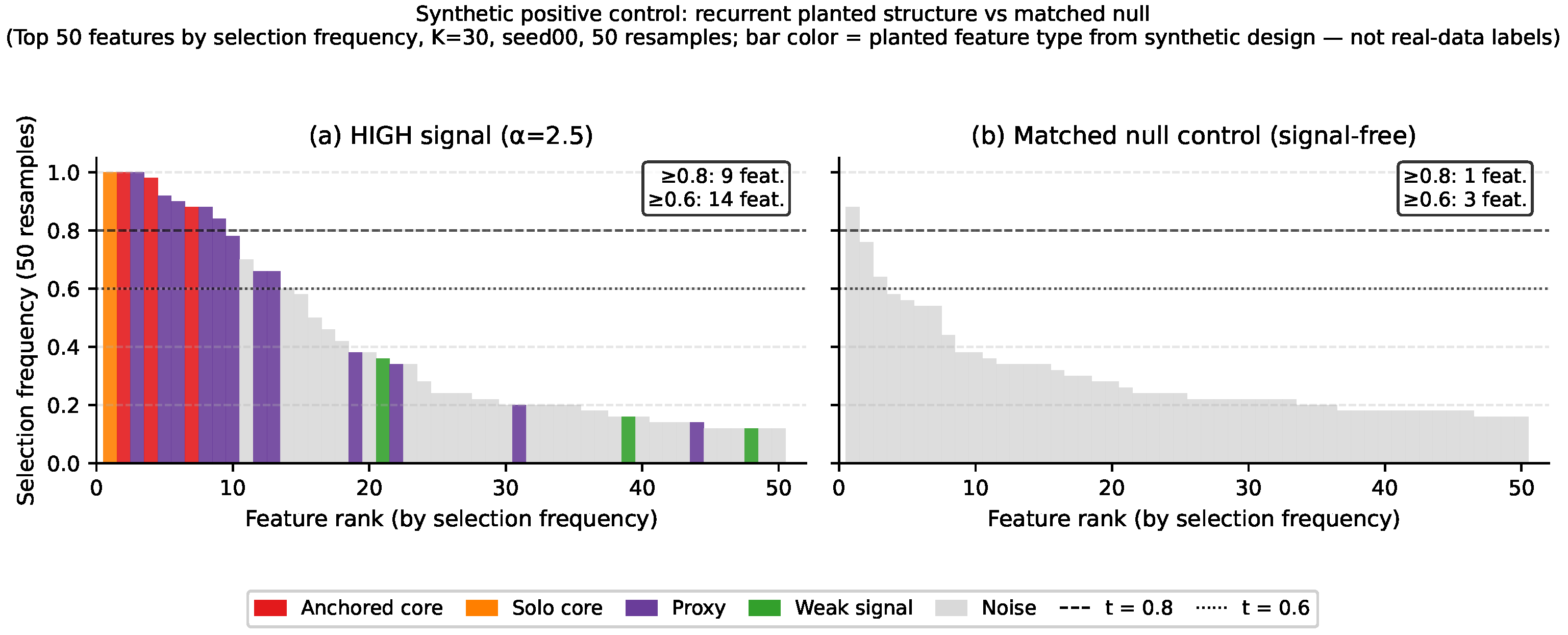
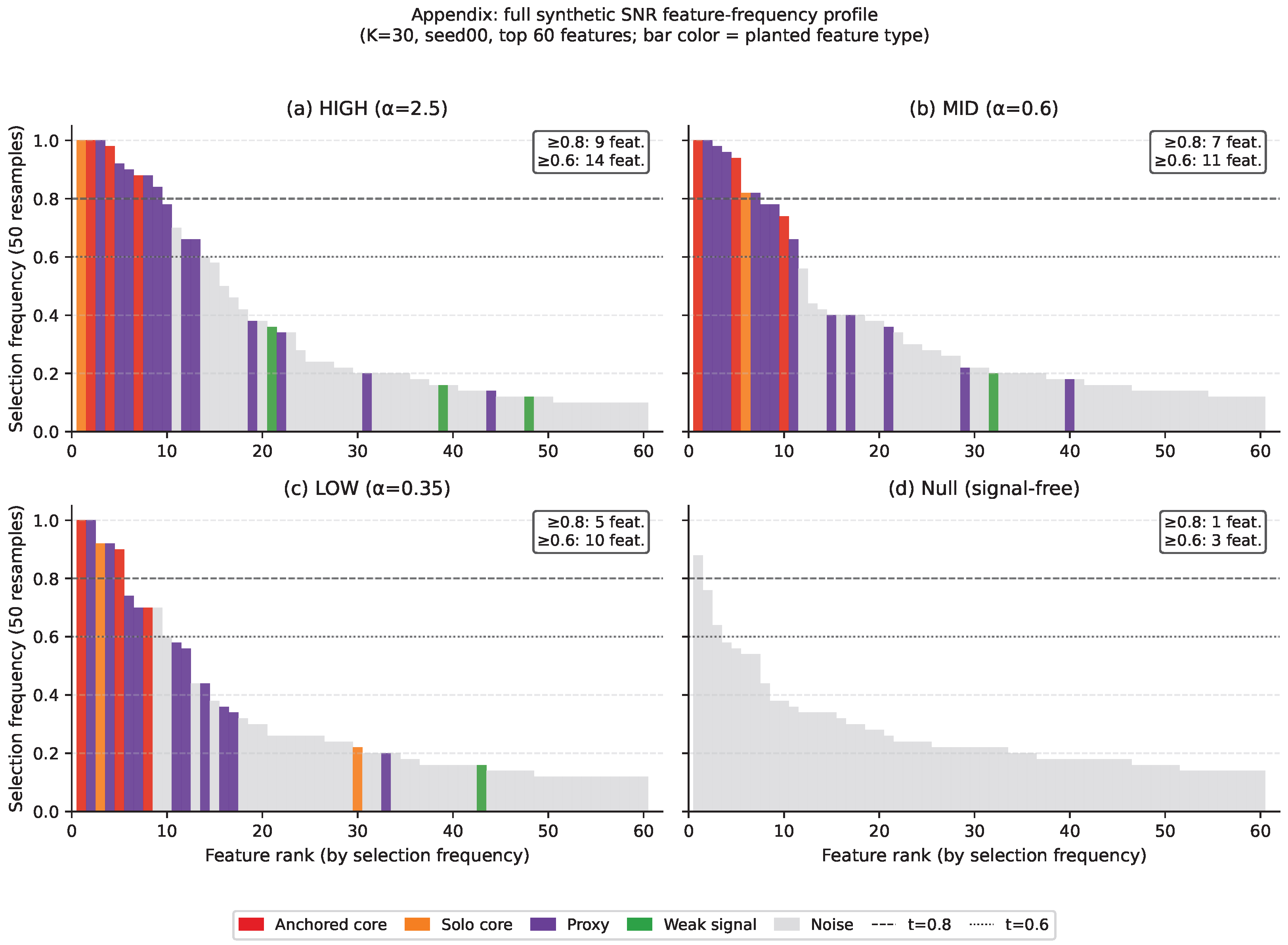
The synthetic study serves as an internal-validity check: because the informative features are planted by construction, a selection can be compared directly against a known support, and recovery can be measured rather than merely inferred. At strong signal, the profile recovered the planted structure. The planted core features recurred at a high selection frequency and separated clearly from the long tail of noise features, whereas the matched null, in which no feature carries signal, produced no comparable recurrent structure (Figure 2; the full panel across all signal levels appears in Appendix A, Figure A1). When the signal is strong, the recurrent candidate core identified by the profile corresponds to the planted core.

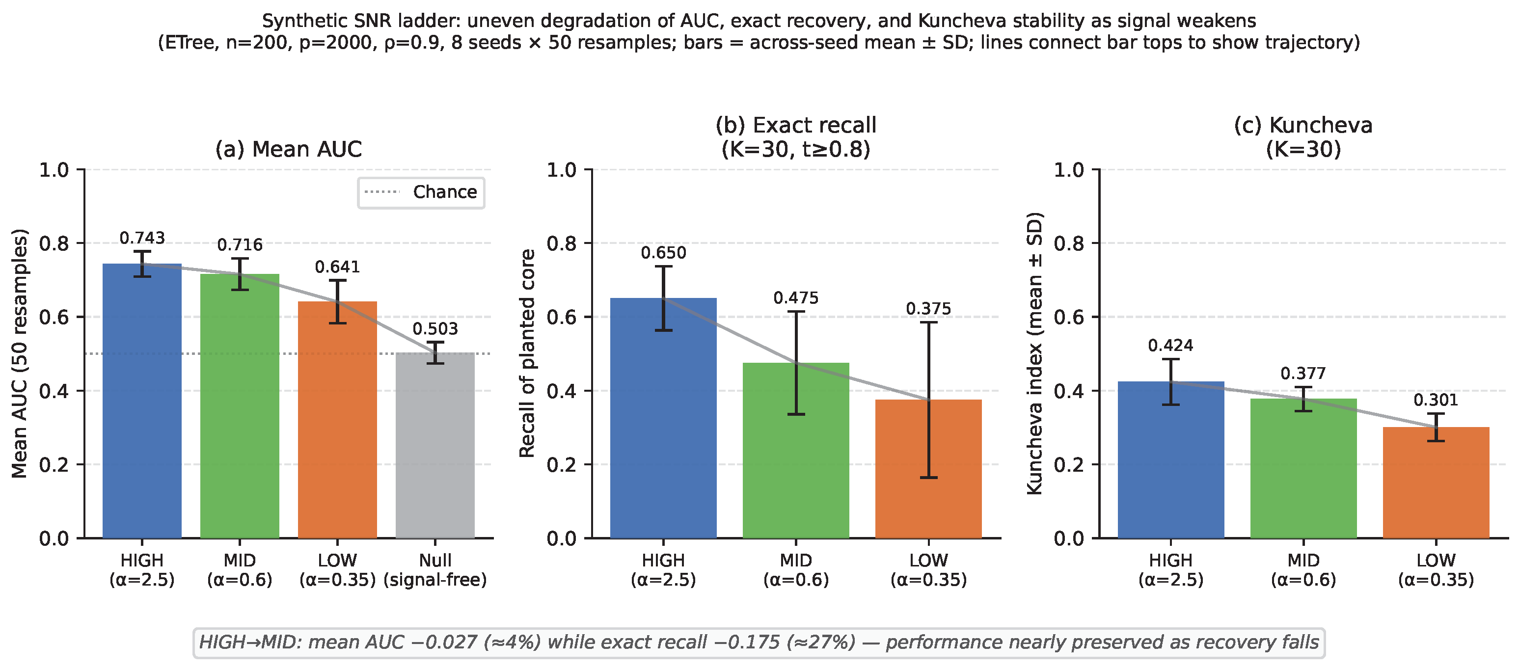
As the signal-strength factor $\alpha$ was reduced, held-out AUC, exact true-core recall, and the chance-corrected stability index all declined, but at visibly different rates, and each remained above its matched-null value throughout (Figure 3). Held-out AUC declined from $0.743$ at strong signal to $0.716$ at the intermediate level and $0.641$ at the weakest, against a null of $0.503$; exact true-core recall ($K=30$, threshold $\tau \ge 0.8$) fell from $0.650$ to $0.475$ to $0.375$; and the Kuncheva index ($K=30$) fell from $0.424$ to $0.377$ to $0.301$, above its null value of $0.202$. The decline was monotone but uneven, the three axes losing ground at different rates rather than in lockstep.

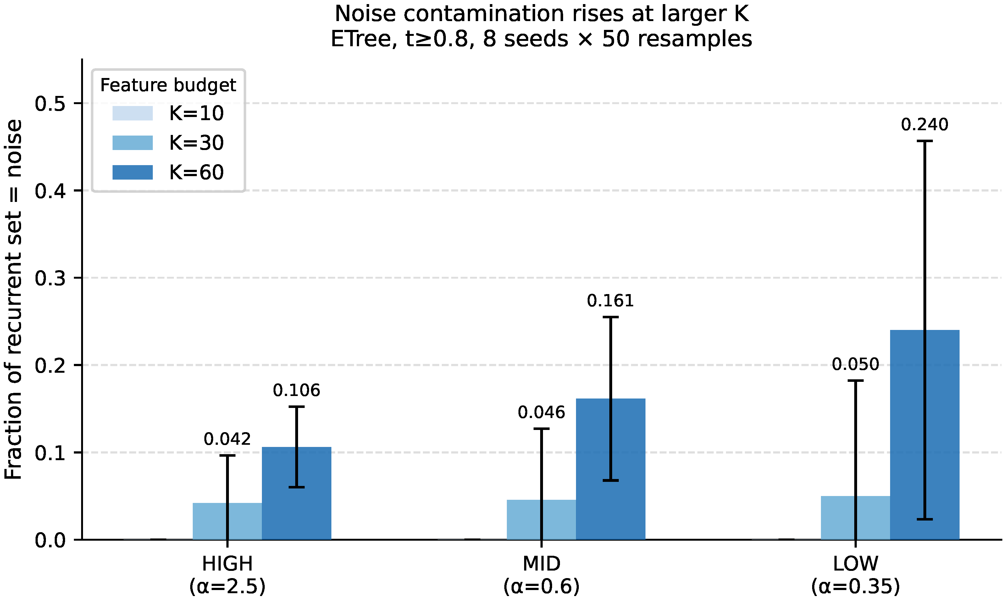
The divergence was sharpest between the strong and intermediate levels. There, held-out AUC was nearly preserved (a change of roughly $0.03$, from $0.743$ to $0.716$) while exact recall of the planted core fell substantially, from $0.650$ to $0.475$. In this controlled setting, predictive performance can be largely retained even as recovery of the planted features weakens. Two further features of the recovery behaviour are worth noting. First, recovery was redundancy-sensitive: proxy-group coverage exceeded exact true-core recall at the two stronger signal levels ($0.750$ versus $0.650$ and $0.667$ versus $0.475$) and matched it at the weakest ($0.375$ versus $0.375$), a pattern consistent with substitution among the redundant proxies planted for each anchored core feature rather than with a failure to capture the signal. Second, at the weakest signal, recovery became strongly instance-dependent: per-seed exact recall ranged from $0.00$ to $0.60$ across the eight generation seeds, so that whether the planted core was recovered depended on the particular data instance. Noise contamination of the recurrent set, by contrast, remained near zero throughout at $K=30$ and $\tau \ge 0.8$ (approximately $0.04$ to $0.05$); it rose only at larger feature budgets, reaching approximately $0.10$ at $K=60$ across signal levels (Appendix A, Figure A2), a budget-sensitivity effect that supports the interpretation that the principal reporting budget is below the noise-entry regime.

Jointly, these results show that, under planted support, predictive performance, subset stability, and support recovery can diverge rather than move together. Because the strong-signal regime is a deliberately strengthened positive-control anchor, the gradient is best read as an internal-validity check of the profile rather than as a representative real-data difficulty, and the recovery quantities reported here are meaningful only because the support is planted. Whether a comparable divergence appears on real data, where no planted support is available, is the subject of the next subsection.

4.2. Real-Data Illustrative Application

We now apply the same frequency-profile logic introduced in the synthetic study to three real datasets, where no planted support exists; accordingly, we make no recovery claim and treat selected features only as recurrent candidates revealed under resampling. Each selector was refit across 50 resamples (seed 0, raw signed X), and we report held-out AUC alongside mean Jaccard overlap and the chance-corrected Kuncheva recurrence index for a compact fixed $K=10$ real-data slice over the three core datasets, summarized in

Table 2. Core real-data stability summary at $K=10$ using 50 resamples, seed 0, and raw signed features. AUC is reported beside mean Jaccard overlap and Kuncheva stability; the table is an illustrative slice, not a benchmark ranking.

Dataset	Algorithm	Resamples	AUC (Mean)	Jaccard (Mean)	Kuncheva
colon	ETree	50	0.868	0.329	0.482
colon	mRMR	50	0.882	0.270	0.414
colon	ReliefF	50	0.830	0.219	0.346
colon	LASSO_Stability	50	0.862	0.154	0.244
SMK-CAN-187	ETree	50	0.719	0.139	0.237
SMK-CAN-187	mRMR	50	0.755	0.092	0.161
SMK-CAN-187	ReliefF	50	0.742	0.181	0.295
SMK-CAN-187	LASSO_Stability	50	0.770	0.247	0.386
PeriodChanger	ETree	50	0.551	0.177	0.286
PeriodChanger	mRMR	50	0.556	0.102	0.172
PeriodChanger	ReliefF	50	0.589	0.132	0.210
PeriodChanger	LASSO_Stability	50	0.597	0.086	0.144

. The value $K=10$ is used as a common reporting budget for this illustrative slice, not as an optimized or recommended feature-budget choice.

The clearest illustration of why these two axes warrant separate reporting comes from colon at $K=10$. There, ETree reached an AUC of $0.868$ with a Kuncheva index of $0.482$, while LASSO_Stability reached an AUC of $0.862$ with a Kuncheva index of $0.244$. The two selectors thus delivered near-identical held-out discrimination, yet their chance-corrected recurrence differed roughly twofold. Read within this dataset and across these algorithms, the pair shows that comparable predictive accuracy can coexist with markedly different stability: a held-out AUC alone would not have surfaced this divergence, whereas the recurrence axis renders it visible.

The within-dataset, across-selector view is consistent across the three datasets. Comparing ETree and mRMR at $K=10$, the Kuncheva index for mRMR was not the larger of the two on any of the three datasets (colon: $0.414$ versus $0.482$; SMK-CAN-187: $0.161$ versus $0.237$; PeriodChanger: $0.172$ versus $0.286$). We report this as an observed pattern in recurrence behaviour, not as a quality ordering between the two selectors.

A second contrast appears across dataset profiles rather than across selectors. Colon presents both higher recurrence and higher AUC (Kuncheva indices roughly $0.24$ to $0.48$, AUC roughly $0.83$ to $0.88$), whereas PeriodChanger presents lower recurrence together with weak discrimination (Kuncheva indices roughly $0.14$ to $0.29$, AUC roughly $0.55$ to $0.60$). We read this as a difference in the descriptive signal each dataset offers under resampling, not as a ranking of the datasets themselves.

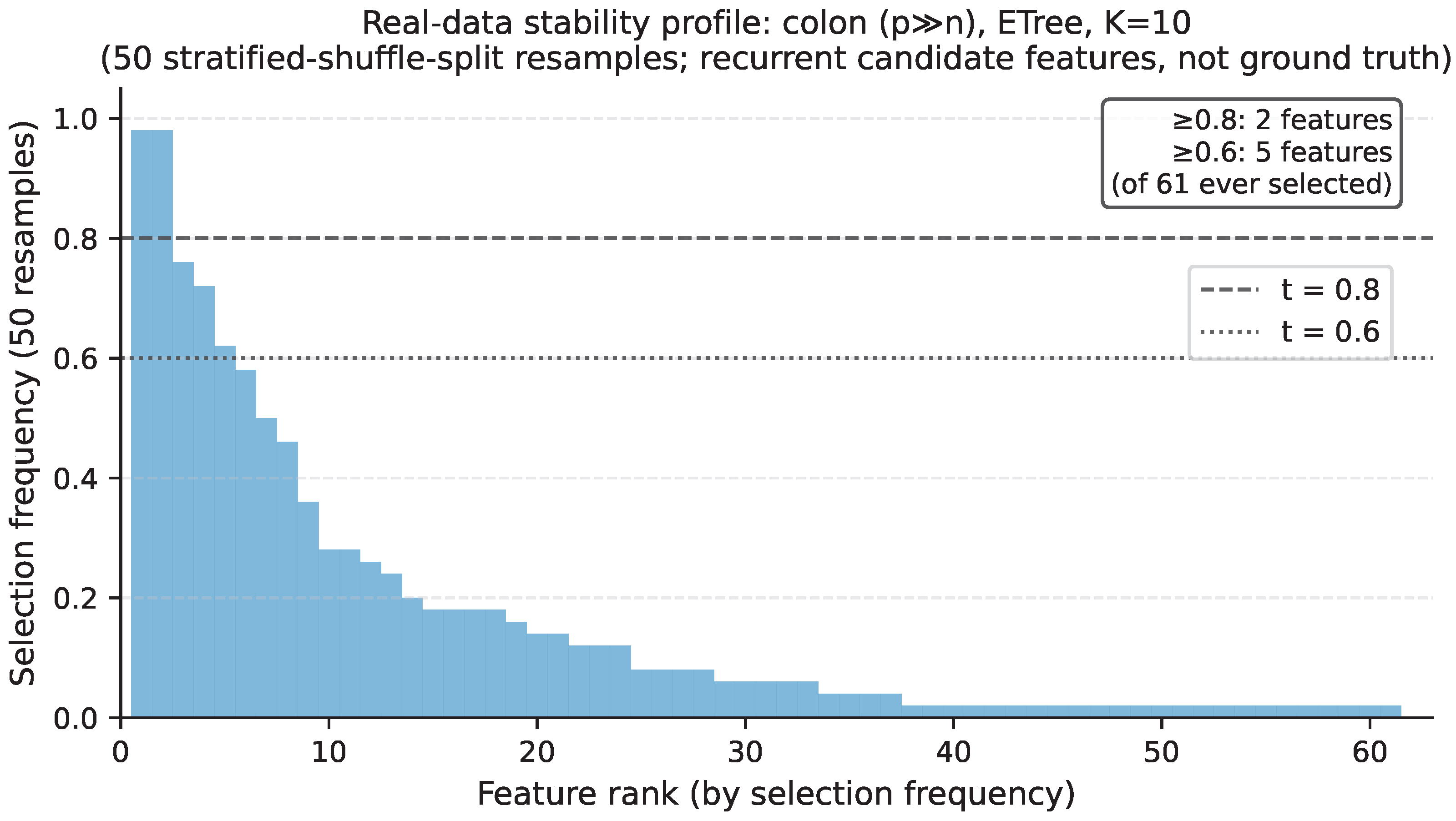
The frequency profile underlying these indices is shown for colon ETree at $K=10$ in Figure 4. Across the resamples, 61 features were selected at least once; of these, 2 recurred in at least a fraction $\tau \ge 0.8$ of resamples and 5 in at least $\tau \ge 0.6$. The profile is therefore one of a small recurrent candidate core embedded within a larger rotating periphery.

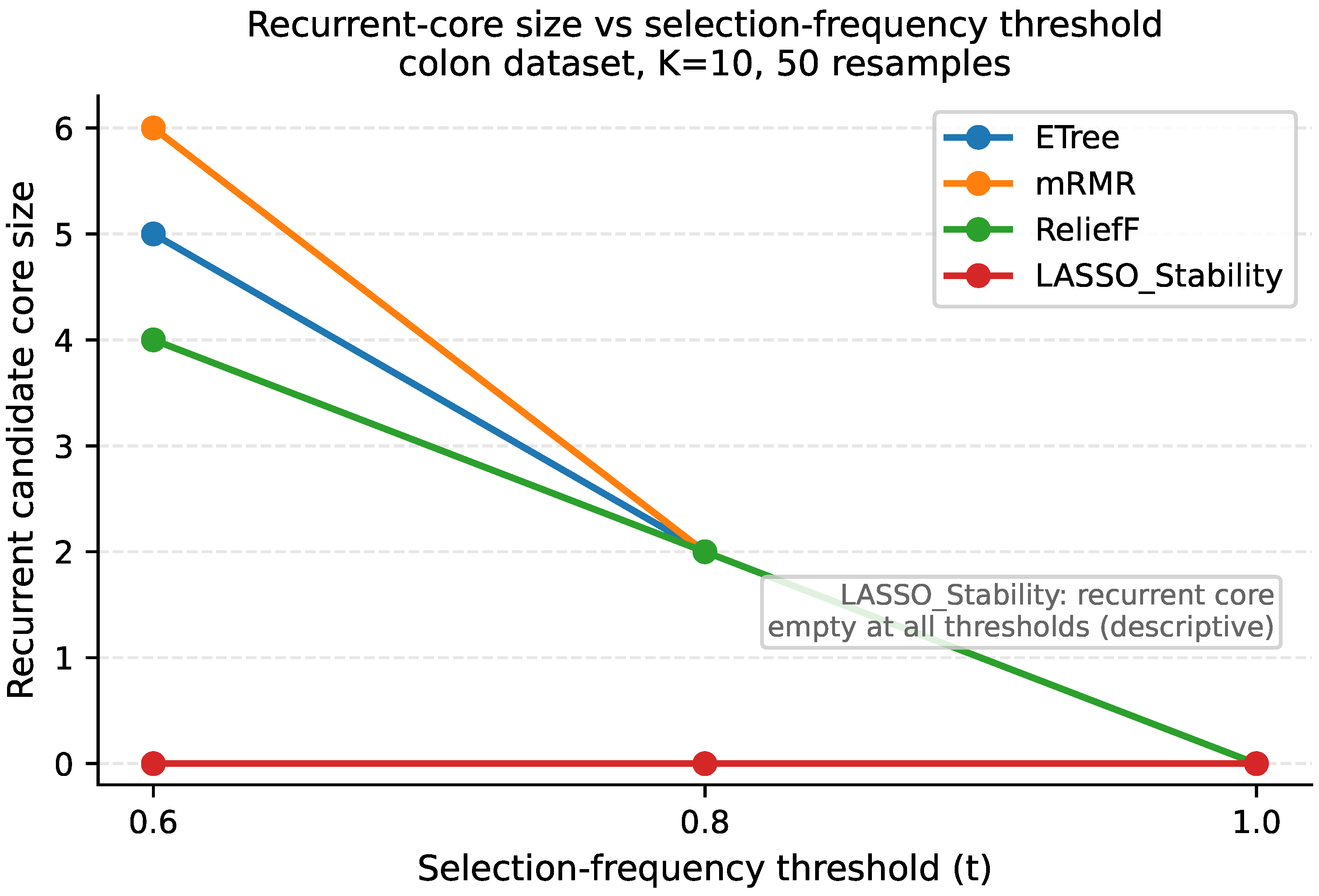
Two appendix extensions situate these observations. Appendix B, Figure A3 sweeps the descriptive recurrence cutoff on colon and shows that the recurrent-set size depends on the chosen threshold, a sensitivity of the descriptive cutoff rather than a form of error control. Appendix B,

Table A1. Full core real-data stability table at $K=10$, including the observed-versus-random ratio. The observed-versus-random ratio is interpreted within dataset only. ^† Obs/Rand ratio is p-dependent; valid for within-dataset comparison only, not for cross-dataset ranking.

Dataset	Algorithm	Resamples	AUC	Jaccard	Kuncheva	Obs/Rand †
colon	ETree	50	0.868	0.329	0.482	131.4
colon	mRMR	50	0.882	0.270	0.414	107.9
colon	ReliefF	50	0.830	0.219	0.346	87.5
colon	LASSO_Stability	50	0.862	0.154	0.244	61.5
SMK-CAN-187	ETree	50	0.719	0.139	0.237	557.7
SMK-CAN-187	mRMR	50	0.755	0.092	0.161	366.1
SMK-CAN-187	ReliefF	50	0.742	0.181	0.295	724.5
SMK-CAN-187	LASSO_Stability	50	0.770	0.247	0.386	987.0
PeriodChanger	ETree	50	0.551	0.177	0.286	41.5
PeriodChanger	mRMR	50	0.556	0.102	0.172	24.0
PeriodChanger	ReliefF	50	0.589	0.132	0.210	31.0
PeriodChanger	LASSO_Stability	50	0.597	0.086	0.144	20.1

provides the full core real-data table and adds the observed-versus-random recurrence ratio, which depends on the candidate-pool size p and is interpreted strictly within a dataset, never to rank datasets against one another. The appendix extension asks whether the same descriptive patterns persist across a broader binary roster.

4.3. Exploratory Analysis Across a Broader Binary Roster

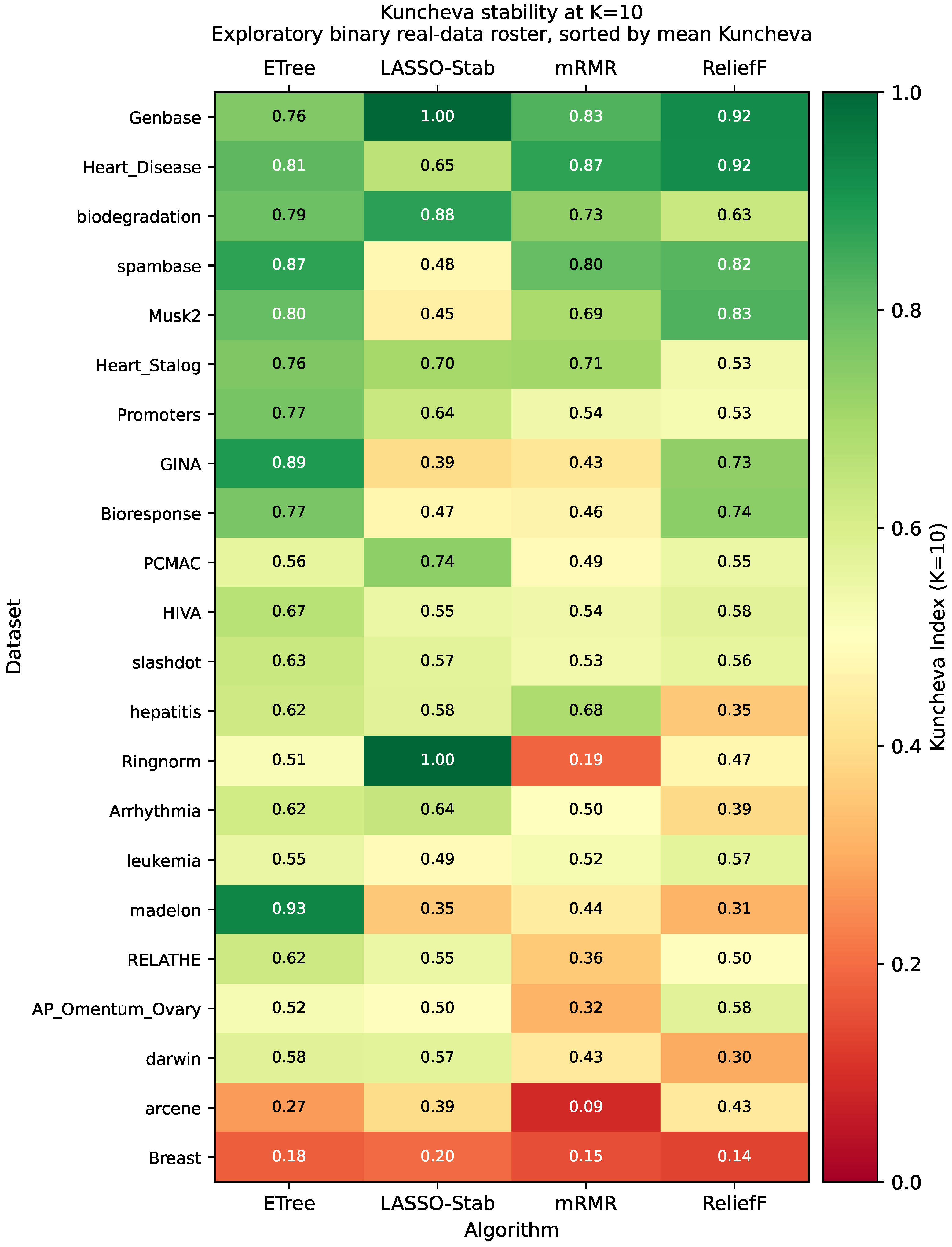
To assess whether the descriptive patterns observed on the three core real-data datasets are peculiar to them, we profiled a broader exploratory roster of 22 further binary datasets eligible at the common $K=10$ reporting slice; multi-class datasets were gated off and fall outside the reported analysis. These datasets appear in Appendix D,

Table A2. Exploratory binary real-data $K=10$ summary. The three core datasets and the 22 further binary datasets eligible at $K=10$ are shown (25 datasets in total). Multi-class datasets are outside the reported analysis. All binary cells completed all 50 resamples.

Dataset	Algorithm	Resamples	AUC	Kuncheva	Jaccard
colon	ETree	50	0.868	0.482	0.329
colon	LASSO_Stability	50	0.862	0.244	0.154
colon	mRMR	50	0.882	0.414	0.270
colon	ReliefF	50	0.830	0.346	0.219
PeriodChanger	ETree	50	0.551	0.286	0.177
PeriodChanger	LASSO_Stability	50	0.597	0.144	0.086
PeriodChanger	mRMR	50	0.556	0.172	0.102
PeriodChanger	ReliefF	50	0.589	0.210	0.132
SMK-CAN-187	ETree	50	0.719	0.237	0.139
SMK-CAN-187	LASSO_Stability	50	0.770	0.386	0.247
SMK-CAN-187	mRMR	50	0.755	0.161	0.092
SMK-CAN-187	ReliefF	50	0.742	0.295	0.181
AP_Omentum_Ovary [27]	ETree	50	0.847	0.522	0.362
AP_Omentum_Ovary	LASSO_Stability	50	0.862	0.496	0.339
AP_Omentum_Ovary	mRMR	50	0.851	0.315	0.192
AP_Omentum_Ovary	ReliefF	50	0.852	0.575	0.415
Arrhythmia [42]	ETree	50	0.765	0.616	0.470
Arrhythmia	LASSO_Stability	50	0.807	0.640	0.496
Arrhythmia	mRMR	50	0.787	0.504	0.364
Arrhythmia	ReliefF	50	0.757	0.389	0.266
Bioresponse [43]	ETree	50	0.787	0.766	0.631
Bioresponse	LASSO_Stability	50	0.780	0.469	0.316
Bioresponse	mRMR	50	0.798	0.463	0.313
Bioresponse	ReliefF	50	0.791	0.739	0.597
Breast [44]	ETree	50	0.705	0.178	0.101
Breast	LASSO_Stability	50	0.725	0.197	0.113
Breast	mRMR	50	0.729	0.149	0.082
Breast	ReliefF	50	0.688	0.136	0.077
GINA [45]	ETree	50	0.866	0.894	0.816
GINA	LASSO_Stability	50	0.848	0.391	0.255
GINA	mRMR	50	0.885	0.425	0.285
GINA	ReliefF	50	0.840	0.733	0.591
Genbase [46]	ETree	50	1.000	0.757	0.619
Genbase	LASSO_Stability	50	1.000	1.000	1.000
Genbase	mRMR	50	1.000	0.827	0.714
Genbase	ReliefF	50	1.000	0.924	0.864
HIVA [45]	ETree	50	0.624	0.666	0.514
HIVA	LASSO_Stability	50	0.633	0.549	0.394
HIVA	mRMR	50	0.669	0.540	0.386
HIVA	ReliefF	50	0.660	0.576	0.421
Heart_Disease [47]	ETree	50	0.932	0.810	0.920
Heart_Disease	LASSO_Stability	50	0.928	0.655	0.857
Heart_Disease	mRMR	50	0.933	0.872	0.946
Heart_Disease	ReliefF	50	0.938	0.918	0.966
Heart_Stalog [48]	ETree	50	0.891	0.758	0.899
Heart_Stalog	LASSO_Stability	50	0.890	0.695	0.873
Heart_Stalog	mRMR	50	0.890	0.707	0.877
Heart_Stalog	ReliefF	50	0.888	0.535	0.813
Musk2 [49]	ETree	50	0.882	0.801	0.691
Musk2	LASSO_Stability	50	0.878	0.452	0.333
Musk2	mRMR	50	0.904	0.691	0.570
Musk2	ReliefF	50	0.888	0.831	0.733
PCMAC [2]	ETree	50	0.697	0.560	0.400
PCMAC	LASSO_Stability	50	0.894	0.738	0.596
PCMAC	mRMR	50	0.817	0.490	0.346
PCMAC	ReliefF	50	0.637	0.548	0.404
Promoters [50]	ETree	50	0.961	0.772	0.690
Promoters	LASSO_Stability	50	0.919	0.636	0.557
Promoters	mRMR	50	0.929	0.541	0.456
Promoters	ReliefF	50	0.948	0.527	0.444
RELATHE [2]	ETree	50	0.696	0.624	0.464
RELATHE	LASSO_Stability	50	0.761	0.550	0.389
RELATHE	mRMR	50	0.767	0.356	0.229
RELATHE	ReliefF	50	0.592	0.496	0.374
Ringnorm [51]	ETree	50	0.965	0.515	0.619
Ringnorm	LASSO_Stability	50	0.968	1.000	1.000
Ringnorm	mRMR	50	0.964	0.191	0.442
Ringnorm	ReliefF	50	0.965	0.470	0.590
arcene [52]	ETree	50	0.787	0.271	0.164
arcene	LASSO_Stability	50	0.795	0.393	0.254
arcene	mRMR	50	0.780	0.088	0.049
arcene	ReliefF	50	0.777	0.432	0.308
biodegradation [53]	ETree	50	0.850	0.789	0.733
biodegradation	LASSO_Stability	50	0.900	0.876	0.834
biodegradation	mRMR	50	0.870	0.734	0.676
biodegradation	ReliefF	50	0.873	0.634	0.576
darwin	ETree	50	0.847	0.581	0.427
darwin	LASSO_Stability	50	0.849	0.572	0.420
darwin	mRMR	50	0.854	0.429	0.295
darwin	ReliefF	50	0.807	0.299	0.193
hepatitis	ETree	50	0.710	0.620	0.705
hepatitis	LASSO_Stability	50	0.718	0.575	0.673
hepatitis	mRMR	50	0.719	0.681	0.744
hepatitis	ReliefF	50	0.696	0.353	0.539
leukemia	ETree	50	0.993	0.553	0.391
leukemia	LASSO_Stability	50	0.992	0.491	0.335
leukemia	mRMR	50	0.994	0.524	0.363
leukemia	ReliefF	50	0.995	0.570	0.410
madelon	ETree	50	0.719	0.934	0.883
madelon	LASSO_Stability	50	0.558	0.354	0.231
madelon	mRMR	50	0.650	0.443	0.300
madelon	ReliefF	50	0.667	0.314	0.202
slashdot	ETree	50	0.621	0.632	0.476
slashdot	LASSO_Stability	50	0.617	0.573	0.413
slashdot	mRMR	50	0.620	0.533	0.376
slashdot	ReliefF	50	0.503	0.560	0.413
spambase	ETree	50	0.880	0.872	0.815
spambase	LASSO_Stability	50	0.853	0.478	0.423
spambase	mRMR	50	0.889	0.798	0.723
spambase	ReliefF	50	0.885	0.817	0.744

and Appendix C, Figure A4. This extension is exploratory appendix support rather than a benchmark: it provides breadth across a wide range of datasets, and no ranking of selectors or datasets is drawn from it. The broad patterns of Section 4.2 persisted across the roster (Appendix D, Table A2). Held-out AUC and chance-corrected recurrence again varied within and across datasets rather than moving together; ETree yielded one of the more consistent recurrent-profile shapes across many of the datasets; and mRMR was, in general, no more recurrent than ETree, echoing the core real-data observation rather than overturning it. The heatmap further summarizes how chance-corrected recurrence varies across datasets and selectors at the common $K=10$ reporting slice (Appendix C, Figure A4).

One caveat accompanies the roster: a subset of K-value combinations are excluded by the pre-specified gating protocol. Cells where K exceeds the number of candidate features or $K>\lfloor 0.64n\rfloor$ are skipped and excluded from the analysis (Appendix D,

Table A3. Skipped-K cells for the exploratory binary real-data roster. All binary cells that passed the pre-specified gating criteria completed all 50 resamples; no partial timeout cells remain. Skipped cells are those where K exceeds the number of candidate features or $K>\lfloor 0.64n\rfloor$.

Dataset	Algorithm	K	Done	Kept	Note
Heart_Disease	all	30, 60	—	no	$K>n_{\mathrm{features}}=13$
Heart_Stalog	all	30, 60	—	no	$K>n_{\mathrm{features}}=13$
Promoters	all	60	—	no	$K=60>n_{\mathrm{features}}=59$
Ringnorm	all	30, 60	—	no	$K>n_{\mathrm{features}}=20$
biodegradation	all	60	—	no	$K=60>n_{\mathrm{features}}=41$
hepatitis	all	30, 60	—	no	$K>n_{\mathrm{features}}=19$
leukemia	all	60	—	no	$K=60>\lfloor 0.64\times 72\rfloor =46$
spambase	all	60	—	no	$K=60>n_{\mathrm{features}}=57$

). All remaining binary cells completed all 50 resamples. As before, the observed-versus-random ratio is read strictly within each dataset. Together, the synthetic, real-data, and appendix results motivate the discussion of feature-stability profiles as a diagnostic layer rather than as a replacement for predictive evaluation.

5. Discussion

5.1. Feature Stability as a Diagnostic Layer

A held-out performance score certifies one property of a feature selection: that the subset it returns supports accurate prediction on unseen data. It says nothing about a second property that becomes important the moment the subset is treated as an explanation of which variables matter: whether the same subset would be returned again under a reasonable perturbation of the data. The results reported above suggest that these two properties are genuinely separable. In the real-data application of Section 4.2, two selectors applied to the same dataset reached near-equal held-out AUC yet differed by roughly twofold in chance-corrected recurrence; the performance score alone would have registered the two selections as essentially equivalent, whereas the recurrence axis revealed that they reselected the same features to very different degrees. We interpret this as the central motivation for the stability profile: it records the reliability axis that performance leaves unmeasured, and we propose that it be reported beside predictive performance as a diagnostic layer rather than in place of it.

The profile is assembled entirely from established measures (the per-feature selection frequency across resamples, the chance-corrected Kuncheva index, and a comparison against a random-selection baseline) and it is read together with the held-out performance recorded on the same resamples. We introduce no new scalar to be optimized and no new selector; the aim is to make performance and recurrence visible together. The contribution is instead integrative and diagnostic: by computing these familiar quantities on the output of a selector as it is ordinarily applied, and by placing them beside performance, the profile makes visible distinctions (such as the colon contrast above) that a single predictive number does not. Understood in this way, feature stability is complementary to predictive evaluation, not a substitute for it: it does not certify that any particular feature is correct, only that performance and recurrence can diverge and that both are worth seeing. The controlled synthetic study clarifies how far these axes can come apart, and why.

5.2. Divergence of Performance, Recovery, and Stability Under Controlled Signal

The synthetic study reported in Section 4.1 occupies a special position in the argument: it is the only setting in which support recovery can be measured rather than merely inferred, because the informative features are planted by construction. Under that planted support, the results indicate that held-out performance, subset stability, and exact support recovery can diverge rather than move as one. As the signal strength was reduced, all three quantities declined, but they declined at visibly different rates, so that the value of any one of them was a poor proxy for the others. This uneven decline is the first sense in which the axes come apart.

The intermediate signal level illustrates the divergence most directly. There, held-out AUC was nearly preserved while exact recovery of the planted core fell materially. We interpret this to mean that, in this controlled setting, a selection can remain predictively useful even as the particular planted features it identifies are recovered less reliably, precisely the situation in which a performance score, taken alone, would give a falsely reassuring picture of the selection. This is the clearest internal-validity case for reading recovery and stability alongside performance wherever a known support makes recovery computable. Two additional patterns refine rather than complicate this reading. First, at the two stronger signal levels, proxy-group coverage exceeded exact true-core recall; a low exact overlap therefore need not signal that the underlying signal was lost, since in this design it can partly reflect substitution among the redundant proxy features planted as near-equivalent alternatives to each core feature. We are careful not to treat those proxies as a truer target than the core: they are redundant alternatives, and the distinction between substitution and genuine loss is itself part of what the profile is meant to expose. Second, at the weakest signal, recovery became instance-dependent across the generation seeds: whether the planted core was recovered depended appreciably on the particular data realization. Throughout, noise contamination of the recurrent set remained low under the reported threshold, which matters for the interpretation: the axes separated not because the profile degenerated into pure noise, but because exact recovery, proxy substitution, and seed dependence each responded differently to weakening signal. Because the strong-signal regime is a deliberately strengthened positive-control anchor rather than a representative level of difficulty, we read these findings as an internal-validity demonstration of how far the axes can come apart under controlled conditions, not as a statement about how often they do so on real data. The real-data setting removes the planted support, and therefore changes what the same profile can and cannot mean.

5.3. Recurrent Candidates on Real Data

The move to real data is a change in kind, not only in degree. In the synthetic study, a planted support made recovery a measurable quantity; on real data no such support exists, and there is consequently nothing against which a selection could be checked for correctness. Recovery is therefore not computable here, and we are careful to read the profile in a strictly descriptive register: the features that recur across resamples are recurrent candidates (features the selector returns consistently under perturbation) and not true, recovered, causal, or validated features. What the profile continues to offer, even without ground truth, is a descriptive trust signal: an account of how stable a selector’s output is.

Predictive performance does not determine the recurrence profile. As already noted in Section 4.2, two selectors reached near-equal held-out AUC on the same dataset yet differed by about twofold in chance-corrected recurrence. The frequency view of such a selection (a small recurrent candidate core embedded within a larger rotating periphery) describes what persists across resamples. These profiles were, moreover, dataset- and selector-dependent: the redundancy-aware selector was not more recurrent than the ensemble selector across the three core datasets, and the datasets themselves differed in their joint performance–recurrence shape. We read these as descriptive contrasts in observed behaviour, and not as a ranking of selectors or of datasets.

Reported beside performance, the recurrence profile records a reliability axis that a performance score leaves unmeasured: a contrast a performance number, taken in isolation, would miss. These observations lead naturally to practical guidance about what should be reported when feature selection is used in high-dimensional studies.

5.4. Implications for Feature-Selection Reporting

These results support a concrete reporting recommendation: feature-selection studies, and high-dimensional studies in particular, would benefit from reporting a stability profile alongside predictive performance rather than reporting performance in isolation. The profile we have in mind requires no new machinery. It places, beside the held-out predictive score, the per-feature selection frequencies estimated across resamples, a chance-corrected stability index such as the Kuncheva index, a recurrent set reported across a sweep of cutoffs rather than fixed at a single arbitrary threshold, and a random-selection baseline interpreted strictly within the dataset at hand. The reporting should also keep two cases distinct: where a planted or externally validated support is available, exact support recovery can be quantified against it; where it is not, the recurrent features should be presented as recurrent candidates, not as recovered or validated ones.

The value of reporting these quantities together is that they separate situations a single summary tends to merge. A profile can distinguish a selection that performs well but recurs unstably from one that achieves similar predictive performance with stronger recurrence; it can distinguish a low subset overlap that reflects benign substitution among redundant alternatives from a low overlap that reflects genuine instability or collapse; and it can make explicit the common configuration of a small recurrent candidate core sitting within a larger rotating periphery. Crucially, the profile does not decide which of these holds on its own. What it offers is a signal that further inspection is warranted, and a sense of what that inspection might involve, for instance, grouping correlated features, checking whether the recurrent candidates are redundant alternatives to one another, or comparing the profiles produced by several plausible selectors on the same data.

It can help to make explicit how these components tend to co-occur.

Table 3. Illustrative, non-exhaustive co-occurrence patterns for reading held-out AUC, chance-corrected recurrence, and frequency-profile shape together. Signal levels are relative within-dataset descriptions, not fixed thresholds.

Pattern	Held-Out AUC	Chance-Corrected Recurrence	Profile Shape	Possible Reading
Performant but low-recurrence	Relatively high	Relatively low	No clear recurrent core; overlap near chance	The features predict, yet the subset varies across resamples; performance does not certify a reproducible selection.
Recurrent and performant	Relatively high	Relatively high	A recurrent candidate core stands out from the periphery	A recurrent candidate core co-occurs with predictive performance under the protocol.
Recurrent core with rotating periphery	Moderate to high	Mixed; low raw overlap with elevated chance-corrected recurrence	A small recurrent core inside a larger rotating periphery	Consistent with redundancy or substitution among correlated proxies; low overlap need not mean lost signal.
No clear pattern	Mixed or unreliable	Mixed or unreliable	Hard to read	Data or protocol limitations prevent a clear reading; no diagnostic conclusion should be drawn.

lists several qualitative patterns that appear in our results when held-out performance, chance-corrected recurrence, and the shape of the frequency profile are read together. The patterns are illustrative rather than exhaustive, and they describe co-occurrences we observed rather than categories the profile assigns: a practitioner reads the three components side by side and may recognize one of these shapes, or none of them. They are not a score, a ranking, or a rule for deciding which selection is correct; their only purpose is to make the joint reading of performance and stability easier to communicate.

The profile is a reporting layer, not a new selection algorithm and not a new summary statistic to be optimized; it makes no claim that one selector or one dataset is preferable to another; and the cutoffs it sweeps are descriptive reporting thresholds that carry no error-control guarantee. Nor does the profile convert recurrent candidates into validated features or substitute for domain validation: it describes how a selection behaves under perturbation and reports that behaviour beside performance, leaving the scientific interpretation to the analyst. In short, the contribution to practice is a more complete description of a selection, not a decision rule. The scope within which these reporting implications hold is set out next.

5.5. Limitations

The scope of the present claim is bounded by several limitations, which we state plainly; each defines an edge of what the study establishes rather than a flaw in what it shows. To begin with, the analysis is restricted to binary classification, and multi-class and regression settings lie outside the present scope. The synthetic design, in turn, is deliberately controlled: its strong-signal regime is a strengthened positive-control anchor, chosen to make recovery legible, not a representative level of real-data difficulty. It therefore supports internal-validity statements about what can happen to the three axes under a known planted support, and not estimates of how frequently such divergence occurs in practice. On real data, the complementary limitation applies: there is no feature-level ground truth, so recovery cannot be computed, and the features that recur are recurrent candidates rather than recovered ones.

The broader evidence carries its own bounds. The broader roster is exploratory appendix support, not a benchmark. The selector set is likewise limited, with four selectors in the real-data application (ETree, mRMR, ReliefF, and LASSO_Stability) and a single ensemble selector in the synthetic study, so the findings should not be read as a complete survey of feature-selection methods. The experimental protocol, too, is held fixed: a single resampling scheme, a fixed random seed, and a fixed budget grid. Other reasonable protocol choices could yield differently shaped profiles, and we do not claim that the particular profiles reported here are protocol-invariant.

Finally, the stability summaries themselves have a bounded interpretation. Because the fixed-budget protocol makes the Nogueira variance-based estimator algebraically equivalent to the mean pairwise Kuncheva index, the results tables report Kuncheva as the single chance-corrected stability summary. The observed-versus-random ratio depends on the size of the candidate pool and is meaningful only within a dataset; and the recurrence cutoffs are descriptive reporting thresholds that carry no false-discovery or family-wise error-control interpretation. These boundaries also fix what the paper is not: a selector, a metric, a benchmark ranking, or an error-controlled procedure. The results should be read accordingly: as a controlled demonstration that performance, stability, and recovery can diverge, together with a descriptive real-data illustration of the same separation between performance and recurrence. Understood within these limits, the limitations bound the scope of the claim without altering its diagnostic interpretation: that the reliability of a selection is worth reporting beside its predictive performance. These limitations point directly to several directions for future work.

5.6. Future Directions

The present framework opens several concrete directions for future work, each of which extends the diagnostic framing rather than departing from it. The most immediate is to extend the stability profile beyond binary classification. Multi-class and regression tasks, and possibly time-to-event settings, are natural targets; each would require adapting the predictive and recurrence summaries to the task at hand, but the underlying structure (a recurrence profile reported beside a performance score) transfers directly, and characterizing how the profile behaves in these settings would broaden the evidence considerably.

A second direction is to profile a wider and mechanistically more varied set of selectors than the few examined here. Embedded, wrapper, model-specific, and regularization-based methods, together with stability-selection variants, would each exercise the diagnostic differently, and comparing their profiles on common data would indicate how far the patterns we observed generalize. We note that profiling a stability-selection variant in this way would treat it as one more selector to be characterized; it would not import the formal error-control guarantees such methods are constructed to deliver. A third, and more demanding, direction is to compare recurrent candidates against an external ground truth where it exists: known biomarkers, curated biological pathways, or experimentally validated variables. Such a comparison would test whether features that recur under perturbation also align with independently established references, and it is precisely the kind of validation the present study cannot perform; we therefore frame it as future work and emphasize that it must not be read backwards as a claim that the recurrent candidates reported here are already validated.

Two further directions concern how the profile is used and how its thresholds are justified. On the first, future work may develop stability-aware reporting workflows that make the diagnostic actionable in practice, indicating when correlated features warrant inspection, when redundant features might be grouped, when several plausible selectors should be compared, and when a high-recurrence yet weakly predictive result should be read as a warning. On the second, the descriptive cutoffs used here invite a more principled treatment: future work could connect recurrence thresholds to procedures that come with formal guarantees, such as stability selection, complementary-pair constructions, or knockoff-based error control, although no such guarantee is claimed in the present paper. More generally, the profile could be incorporated into reporting pipelines or analysis dashboards so that the stability of a selection is recorded alongside its performance as a matter of routine practice. These directions preserve the central framing of the present work: feature-stability profiles are most useful when treated as a diagnostic complement to predictive evaluation.

6. Conclusions

Feature selection is conventionally evaluated by the predictive performance of the features it returns, but predictive performance and feature-selection stability answer different questions: the first asks whether the selected subset supports accurate prediction, the second whether the same subset would be returned again under a reasonable perturbation of the data. The central argument of this paper is that both should be reported, and we have proposed a feature-stability profile as the means of reporting the second. The profile is assembled from established quantities (per-feature recurrence across resamples, a chance-corrected stability index, the recurrent set summarized across a sweep of cutoffs rather than at a single threshold, and held-out performance recorded on the same resamples) and is read as a diagnostic layer beside predictive evaluation rather than in place of it.

Two settings clarified what the profile can and cannot say. In a synthetic controlled study, where the informative support is planted by construction and recovery can be measured directly, predictive performance, subset stability, and support recovery can diverge rather than decline in step. On real data, where feature-level ground truth is unavailable, the same profile is necessarily descriptive: the features that recur are recurrent candidates, not recovered or validated ones. So understood, the profile can surface selections that predict well yet recur unstably, selections that recur stably yet predict weakly, small recurrent candidate cores within larger rotating peripheries, and (under controlled support) substitution among redundant alternatives. The contribution is deliberately diagnostic and integrative: it makes a selection’s reliability reportable using only established quantities, and is by design not a new selector, not a new metric, not a benchmark ranking, and not an error-controlled procedure. Reported beside predictive performance, feature-stability profiles make the reliability of a selected feature set visible rather than assumed.

References

1. Guyon, I.; Elisseeff, A. An introduction to variable and feature selection. J. Mach. Learn. Res. 2003, 3, 1157–1182. [Google Scholar]
2. Li, J.; Cheng, K.; Wang, S.; Morstatter, F.; Trevino, R.P.; Tang, J.; Liu, H. Feature Selection: A Data Perspective. ACM Comput. Surv. 2017, 50, 94. [Google Scholar] [CrossRef] [Scilit]
3. Kalousis, A.; Prados, J.; Hilario, M. Stability of Feature Selection Algorithms: A Study on High-Dimensional Spaces. Knowl. Inf. Syst. 2007, 12, 95–116. [Google Scholar] [CrossRef] [Scilit]
4. Takefuji, Y. The Reliability Gap: Why High Predictive Accuracy Doesn’t Guarantee Stable Feature Importance. Mar. Pollut. Bull. 2026, 226, 119398. [Google Scholar] [CrossRef] [Scilit] [PubMed]
5. Yu, B.; Kumbier, K. Veridical Data Science. Proc. Natl. Acad. Sci. USA 2020, 117, 3920–3929. [Google Scholar] [CrossRef] [Scilit] [PubMed]
6. Meinshausen, N.; Bühlmann, P. Stability selection. J. R. Stat. Soc. Ser. B 2010, 72, 417–473. [Google Scholar] [CrossRef] [Scilit]
7. Tanimoto, T.T. An Elementary Mathematical Theory of Classification and Prediction; Internal IBM Technical Report; International Business Machines Corporation: New York, NY, USA, 1958. [Google Scholar]
8. Dice, L.R. Measures of the Amount of Ecologic Association Between Species. Ecology 1945, 26, 297–302. [Google Scholar] [CrossRef] [Scilit]
9. Ochiai, A. Zoogeographical Studies on the Soleoid Fishes Found in Japan and Its Neighbouring Regions. Bull. Jpn. Soc. Sci. Fish. 1957, 22, 526–530. [Google Scholar] [CrossRef] [Scilit]
10. Nogueira, S.; Sechidis, K.; Brown, G. On the Stability of Feature Selection Algorithms. J. Mach. Learn. Res. 2018, 18, 1–54. [Google Scholar]
11. Kuncheva, L.I. A Stability Index for Feature Selection. In Proceedings of the 25th IASTED International Multi-Conference: Artificial Intelligence and Applications; ACTA Press: Anaheim, CA, USA, 2007; pp. 390–395. [Google Scholar]
12. Bommert, A.; Lang, M. stabm: Stability Measures for Feature Selection. J. Open Source Softw. 2021, 6, 3010. [Google Scholar] [CrossRef] [Scilit]
13. Toloşi, L.; Lengauer, T. Classification with Correlated Features: Unreliability of Feature Ranking and Solutions. Bioinformatics 2011, 27, 1986–1994. [Google Scholar] [CrossRef] [Scilit] [PubMed]
14. Zou, H.; Hastie, T. Regularization and Variable Selection via the Elastic Net. J. R. Stat. Soc. Ser. B 2005, 67, 301–320. [Google Scholar] [CrossRef] [Scilit]
15. Saeys, Y.; Abeel, T.; Van de Peer, Y. Robust Feature Selection Using Ensemble Feature Selection Techniques. In Proceedings of the Machine Learning and Knowledge Discovery in Databases; Lecture Notes in Computer Science; Springer: Berlin/Heidelberg, Germany, 2008; Volume 5212, pp. 313–325. [Google Scholar] [CrossRef] [Scilit]
16. Hamer, V.; Dupont, P. An Importance Weighted Feature Selection Stability Measure. J. Mach. Learn. Res. 2021, 22, 1–57. [Google Scholar]
17. Shah, R.D.; Samworth, R.J. Variable Selection with Error Control: Another Look at Stability Selection. J. R. Stat. Soc. Ser. B 2013, 75, 55–80. [Google Scholar] [CrossRef] [Scilit]
18. Tang, J.; Alelyani, S.; Liu, H. Feature selection for classification: A review. In Data Classification: Algorithms and Applications; Aggarwal, C.C., Ed.; CRC Press: Boca Raton, FL, USA, 2014; p. 37. [Google Scholar]
19. Post, M.J.; van der Putten, P.; van Rijn, J.N. Does Feature Selection Improve Classification? A Large Scale Experiment in OpenML. In Proceedings of the Advances in Intelligent Data Analysis XV (IDA 2016); Lecture Notes in Computer Science; Springer: Berlin/Heidelberg, Germany, 2016; Volume 9897, pp. 158–170. [Google Scholar] [CrossRef] [Scilit]
20. Cherepanova, V.; Levin, R.; Somepalli, G.; Geiping, J.; Bruss, C.B.; Wilson, A.G.; Goldstein, T.; Goldblum, M. A Performance-Driven Benchmark for Feature Selection in Tabular Deep Learning. Adv. Neural Inf. Process. Syst. 2023, 36, 41956–41979. [Google Scholar] [CrossRef] [Scilit]
21. Bommert, A.; Sun, X.; Bischl, B.; Rahnenführer, J.; Lang, M. Benchmark for filter methods for feature selection in high-dimensional classification data. Comput. Stat. Data Anal. 2020, 143, 106839. [Google Scholar] [CrossRef] [Scilit]
22. Ambroise, C.; McLachlan, G.J. Selection bias in gene extraction on the basis of microarray gene-expression data. Proc. Natl. Acad. Sci. USA 2002, 99, 6562–6566. [Google Scholar] [CrossRef] [Scilit] [PubMed]
23. Cawley, G.C.; Talbot, N.L.C. On Over-fitting in Model Selection and Subsequent Selection Bias in Performance Evaluation. J. Mach. Learn. Res. 2010, 11, 2079–2107. [Google Scholar]
24. Demircioğlu, A. Measuring the Bias of Incorrect Application of Feature Selection When Using Cross-Validation in Radiomics. Insights Imaging 2021, 12, 172. [Google Scholar] [CrossRef] [Scilit] [PubMed]
25. Chicco, D.; Jurman, G. The Advantages of the Matthews Correlation Coefficient (MCC) over F1 Score and Accuracy in Binary Classification Evaluation. BMC Genom. 2020, 21, 6. [Google Scholar] [CrossRef] [Scilit] [PubMed]
26. Saito, T.; Rehmsmeier, M. The Precision–Recall Plot Is More Informative than the ROC Plot When Evaluating Binary Classifiers on Imbalanced Datasets. PLoS ONE 2015, 10, e0118432. [Google Scholar] [CrossRef] [Scilit] [PubMed]
27. Stiglic, G.; Kokol, P. Stability of ranked gene lists in large microarray analysis studies. BioMed Res. Int. 2010, 2010, 616358. [Google Scholar] [CrossRef] [Scilit]
28. Haury, A.; Gestraud, P.; Vert, J. The influence of feature selection methods on accuracy, stability, and interpretability of molecular signatures. PLoS ONE 2011, 6, e28210. [Google Scholar] [CrossRef] [Scilit] [PubMed]
29. Bolón-Canedo, V.; Alonso-Betanzos, A. Ensembles for Feature Selection: A Review and Future Trends. Inf. Fusion 2019, 52, 1–12. [Google Scholar] [CrossRef] [Scilit]
30. Tibshirani, R. Regression Shrinkage and Selection via the Lasso. J. R. Stat. Soc. Ser. B 1996, 58, 267–288. [Google Scholar] [CrossRef] [Scilit]
31. Peng, H.; Long, F.; Ding, C. Feature selection based on mutual information criteria of max-dependency, max-relevance, and min-redundancy. IEEE Trans. Pattern Anal. Mach. Intell. 2005, 27, 1226–1238. [Google Scholar] [PubMed]
32. Yu, L.; Liu, H. Feature selection for high-dimensional data: A fast correlation-based filter solution. In Proceedings of the 20th International Conference on Machine Learning (ICML-03); AAAI Press: Washington, DC, USA, 2003; pp. 856–863. [Google Scholar]
33. Ho, T.K.; Basu, A. Complexity Measures of Supervised Classification Problems. IEEE Trans. Pattern Anal. Mach. Intell. 2002, 24, 289–300. [Google Scholar] [CrossRef] [Scilit]
34. Lorena, A.C.; Garcia, L.P.F.; Lehmann, J.; de Souto, M.C.P.; Ho, T.K. How Complex Is Your Classification Problem? A Survey on Measuring Classification Complexity. ACM Comput. Surv. 2019, 52, 107. [Google Scholar] [CrossRef] [Scilit]
35. Komorniczak, J.; Ksieniewicz, P. problexity—An Open-Source Python Library for Supervised Learning Problem Complexity Assessment. Neurocomputing 2023, 521, 126–136. [Google Scholar] [CrossRef] [Scilit]
36. Elmakias, I.; Vilenchik, D. Choosing the Right Dataset: Hardness Criteria for Feature Selection Benchmarking. Knowl.-Based Syst. 2025, 334, 115022. [Google Scholar] [CrossRef] [Scilit]
37. Geurts, P.; Ernst, D.; Wehenkel, L. Extremely randomized trees. Mach. Learn. 2006, 63, 3–42. [Google Scholar] [CrossRef] [Scilit]
38. Alon, U.; Barkai, N.; Notterman, D.A.; Gish, K.; Ybarra, S.; Mack, D.; Levine, A.J. Broad patterns of gene expression revealed by clustering analysis of tumor and normal colon tissues probed by oligonucleotide arrays. Proc. Natl. Acad. Sci. USA 1999, 96, 6745–6750. [Google Scholar] [CrossRef] [Scilit] [PubMed]
39. Gül, Ş.; Rahim, F. Period Changer; UCI Machine Learning Repository: Irvine, CA, USA, 2021. [Google Scholar] [CrossRef]
40. Robnik-Šikonja, M.; Kononenko, I. Theoretical and empirical analysis of ReliefF and RReliefF. Mach. Learn. 2003, 53, 23–69. [Google Scholar] [CrossRef] [Scilit]
41. Pedregosa, F.; Varoquaux, G.; Gramfort, A.; Michel, V.; Thirion, B.; Grisel, O.; Blondel, M.; Prettenhofer, P.; Weiss, R.; Dubourg, V.; et al. Scikit-learn: Machine learning in Python. J. Mach. Learn. Res. 2011, 12, 2825–2830. [Google Scholar]
42. Guvenir; Quinlan, R. Arrhythmia; UCI Machine Learning Repository: Irvine, CA, USA, 1997. [Google Scholar] [CrossRef]
43. Vanschoren, J.; Van Rijn, J.N.; Bischl, B.; Torgo, L. OpenML: Networked science in machine learning. ACM SIGKDD Explor. Newsl. 2014, 15, 49–60. [Google Scholar]
44. Pochet, N.; De Smet, F.; Suykens, J.A.; De Moor, B.L. Systematic benchmarking of microarray data classification: Assessing the role of non-linearity and dimensionality reduction. Bioinformatics 2004, 20, 3185–3195. [Google Scholar] [CrossRef] [Scilit] [PubMed]
45. Guyon, I.; Alamdari, A.R.S.A.; Dror, G.; Buhmann, J.M. Performance prediction challenge. In The 2006 IEEE International Joint Conference on Neural Network Proceedings; IEEE: New York, NY, USA, 2006; pp. 1649–1656. [Google Scholar]
46. Diplaris, S.; Tsoumakas, G.; Mitkas, P.A.; Vlahavas, I. Protein classification with multiple algorithms. In Proceedings of the Advances in Informatics: 10th Panhellenic Conference on Informatics, PCI 2005, Volas, Greece, 11–13 November 2005; Proceedings 10; Springer: Berlin/Heidelberg, Germany, 2005; pp. 448–456. [Google Scholar]
47. Zhang, D.; Zou, L.; Zhou, X.; He, F. Integrating feature selection and feature extraction methods with deep learning to predict clinical outcome of breast cancer. IEEE Access 2018, 6, 28936–28944. [Google Scholar] [CrossRef] [Scilit]
48. Mansouri, A. Statlog (Heart); UCI Machine Learning Repository: Irvine, CA, USA, 2010. [Google Scholar] [CrossRef]
49. Chapman, D.; Jain, A. Musk (Version 2); UCI Machine Learning Repository: Irvine, CA, USA, 1994. [Google Scholar] [CrossRef]
50. Yilmaz, B. Müşteri İlişkileri Yönetimi İçin Manifold Öğrenme İle Denetimli Doğrusal Olmayan Boyut İndirgeme. Master’s Thesis, İstanbul Kültür Üniversitesi, Istanbul, Turkey, 2023. [Google Scholar]
51. Breiman, L. Bias, Variance, and Arcing Classifiers; Technical Report 460; Statistics Department, University of California: Berkeley, CA, USA, 1996; Available online: https://statistics.berkeley.edu/sites/default/files/tech-reports/460.pdf (accessed on 24 June 2026).
52. Guyon, I.; Gunn, S.; Ben-Hur, A.; Dror, G. Result analysis of the nips 2003 feature selection challenge. In Advances in Neural Information Processing Systems 17; Saul, L.K., Weiss, Y., Bottou, L., Eds.; MIT Press: Cambridge, MA, USA, 2004; Volume 17. [Google Scholar]
53. Mansouri, K.; Ringsted, T.; Ballabio, D.; Todeschini, R.; Consonni, V. Quantitative structure–activity relationship models for ready biodegradability of chemicals. J. Chem. Inf. Model. 2013, 53, 867–878. [Google Scholar] [CrossRef] [Scilit] [PubMed]
Figure 1. Stability-profiling workflow. Repeated stratified resampling produces B training/evaluation splits; the selector is applied on each training partition at a fixed budget K, with held-out AUC recorded on the evaluation partition; the B selected sets are aggregated into selection-frequency profiles, recurrent sets, stability summaries, and a random-selection baseline. Recovery summaries are computed only in the synthetic setting, where the planted support is known.
Mathematics 14 02372 g001
Figure 2. Synthetic selection-frequency profile at strong signal versus matched null for seed 00 using ETree at K = 30 . Colours denote planted feature roles from the synthetic design, not real-data labels.
Mathematics 14 02372 g002
Figure 3. Synthetic signal-strength gradient across eight generation seeds using ETree at K = 30 , as the signal-strength factor α decreases: (a) held-out AUC, (b) exact true-core recall at τ 0.8 , and (c) the Kuncheva stability index.
Mathematics 14 02372 g003
Figure 4. Descriptive selection-frequency profile for colon using ETree at K = 10 ; recurrent features are reported as candidates only, with no support recovery computed on real data.
Mathematics 14 02372 g004