Interpretable Multivariate Process Monitoring Using MEWMA and Explainable Machine Learning

Abstract

Monitoring the stability of multivariate quality processes is essential for ensuring product conformity and process reliability in industrial systems. Multivariate Exponentially Weighted Moving Average (MEWMA) control charts are widely used to detect small and persistent shifts in correlated quality characteristics. However, although MEWMA can identify out-of-control (OOC) conditions, it does not directly indicate which variables contribute to the detected signal. To address this limitation, this study reformulates multivariate control chart interpretation as an explainable supervised learning problem using data from an automotive production process. Several machine learning classifiers, including XGBoost, Random Forest, Support Vector Machines (SVM), LightGBM, Logistic Regression, CatBoost, and K-Nearest Neighbors (KNN), were trained using In-Control (IC)/OOC labels generated from MEWMA monitoring outcomes. Statistical tests were conducted to examine whether the observed performance differences among classifiers were statistically significant, while the computational efficiency of the framework was evaluated through a per-observation timing experiment. Among the evaluated models, XGBoost provided the most balanced overall classification performance and was further examined using the SHapley Additive exPlanations (SHAP) method. SHAP analysis enabled both global and local interpretations of model predictions by quantifying each variable’s contribution to OOC classifications. The findings indicate that combining MEWMA-based monitoring with explainable machine learning offers a practical and interpretable complement to analytical decomposition approaches in multivariate process monitoring. The proposed approach offers a practical, data-driven framework for explaining MEWMA-based IC/OOC classification decisions and identifying the relative contributions of variables in industrial quality-monitoring applications.

1. Introduction

Modern industrial processes involve numerous interrelated variables, necessitating intelligent and interpretable monitoring systems that go beyond traditional statistical approaches. Statistical process control (SPC) is one of the widely used approaches for monitoring the stability of industrial production processes and ensuring the sustainability of quality levels. SPC aims to evaluate process performance using statistical methods, detect potential shifts early, and eliminate them before they affect product quality [1]. In today’s production systems, processes are generally defined by numerous interrelated variables, and the total variation created by these variables is decisive for the process’s stability. Therefore, when univariate control charts are insufficient, multivariate control charts that account for variable correlations are used. However, in modern production environments, detecting a process shift alone is often insufficient; identifying and interpreting the source of that shift is equally important for effective process intervention and decision-making.

One of the most commonly used methods in this context is the Multivariate Exponentially Weighted Moving Average (MEWMA) control chart, which is highly sensitive to small and medium-sized shifts due to its weighted consideration of past observations. MEWMA stands out as an effective monitoring tool, especially in production systems with complex, large datasets, as it can detect shifts that accumulate over time in the process at an early stage [2]. Despite this strong detection capability, MEWMA does not directly indicate which variables contribute to the detected shift, which limits its usefulness for process interpretation and decision support. In recent years, various Machine Learning (ML) algorithms have been integrated into studies to improve MEWMA performance. For example, Kazmi and Noor-ul-Amin [3] proposed an approach where the smoothing parameter is learned using Random Forest, KNN, and Support Vector Regression algorithms to strengthen the adaptive structure of MEWMA. The results show that the ML-supported MEWMA structure offers lower Average Run Length (ARL) values compared to classical MEWMA. Similarly, Weix et al. [4] used random forests and neural networks to model intervariate dependencies in time series and performed process monitoring using MEWMA based on the resulting residuals. In their study, Sabahno and Amiri [5] comparatively examined statistical control charts, including MEWMA, Hotelling’s T², and LRT (likelihood ratio test), alongside ANN (artificial neural network), SVR (support vector regression), and Random Forest-based ML models. The study showed that ML-based control charts were more successful than statistical methods, especially in detecting small shifts. Yao et al. [6] integrated MEWMA with algorithms such as Random Forest, XGBoost, and LightGBM for fault detection in industrial refrigeration systems. These studies clearly demonstrate that ML integration increases the detection power of control charts. However, these studies primarily focus on improving detection or adaptive monitoring performance, whereas the problem of providing an interpretable explanation of multivariate control chart signals remains insufficiently addressed.

As noted in the literature, MEWMA control charts indicate the presence of an OOC signal in the process but do not directly indicate which variable or variables are responsible for the detected shift [7]. This makes it difficult to identify the responsible variable(s) requiring corrective intervention when an OOC signal is received. Using machine learning models to examine which variables contribute to MEWMA-based OOC classification decisions represents a promising solution. However, the limited interpretability of many ML models, often referred to as the “black-box” problem, restricts their direct applicability in engineering decision support [8]. To overcome this problem, Explainable Artificial Intelligence (XAI) approaches have come to the forefront in recent years. XAI methods aim to make the decision-making mechanisms of ML models transparent, revealing not only what decision was made, but also why it was made. In this context, the SHapley Additive exPlanations (SHAP) method, thanks to its game theory-based structure, can quantify the contribution of each feature to the model output in a consistent and interpretable manner at both local and global levels [9]. Although the SHAP method has been successfully applied in many fields, such as health, energy, reliability analysis, and fault diagnosis, its use for process monitoring—particularly for interpreting machine learning models trained on multivariate control chart outputs—remains limited in the literature [10].

This study addresses this gap by reformulating multivariate control chart interpretation as an explainable supervised learning problem. In the proposed framework, OOC signals are first identified using a MEWMA control chart, and the resulting IC/OOC labels are then used to train machine learning models as a supervised classification problem. This structure makes it possible not only to detect OOC signals, but also to explain which variables contribute to these decisions and to what extent. Accordingly, the proposed approach combines control chart-based detection with model-based explainability to provide an interpretable and data-driven approach for multivariate process monitoring.

The main contributions of this study are as follows:

(1)

Integration of MEWMA-based monitoring with supervised ML for multivariate IC/OOC classification,

(2)

Learning of nonlinear decision boundaries from MEWMA-generated IC/OOC labels using supervised ML models,

(3)

Use of SHAP analysis to explain variable-level contributions to OOC classifications,

(4)

Development of an interpretable and data-driven framework that links IC/OOC classification with explainable ML.

2. Background

2.1. Multivariate Exponentially Weighted Moving Average (MEWMA) Control Chart

The MEWMA control chart, initially proposed by Lowry et al. [11] is one of the most effective techniques for detecting small and sustained shifts in multivariate processes. Unlike Hotelling’s $T^2$ chart, which considers only the most recent sample, the MEWMA chart incorporates information from past observations through an exponential weighting scheme, providing a memory structure that enhances sensitivity to gradual process drifts [12].

Let ${\mathit{x}}_t={\left[x_{1t},x_{2t},\dots ,x_{pt}\right]}^T$ denote the vector of p correlated quality variables at time t, with IC mean vector ${\mathit{\mu }}_0$ and covariance matrix $\mathsf{\Sigma }$. The exponentially weighted moving average statistic is recursively defined as:

$${\mathit{Z}}_t=\lambda {\mathit{x}}_t+\left(1-\lambda \right){\mathit{Z}}_{t-1}, {\mathit{Z}}_0={\mathit{\mu }}_0$$

(1)

where $0<\lambda \le 1$ is the smoothing constant determining how strongly recent observations influence the statistic. Here, ${\mathit{x}}_t$ is the $p\times 1$ observation vector at time $t$, ${\mathit{Z}}_t$ is the MEWMA statistic vector, ${\mathit{\mu }}_{\mathbf{0}}$ is the IC mean vector, and ∑ is the IC covariance matrix. Smaller values of $\lambda$ yield smoother trajectories and greater sensitivity to small, sustained shifts, whereas larger values make the chart more reactive to sudden changes [1].

The monitoring statistic is computed as:

$$T_t^2=({\mathbf{Z}}_t-{\mathit{\mu }}_0{)}^{\mathrm{\top }}{\mathsf{\Sigma }}_Z^{-1}({\mathbf{Z}}_t-{\mathit{\mu }}_0)$$

(2)

Here, $T_t^2$ denotes the MEWMA monitoring statistic and ${\mathsf{\Sigma }}_Z$ is the covariance matrix of ${\mathbf{Z}}_t$, given by:

$${\mathsf{\Sigma }}_Z={\displaystyle \frac{\lambda }{2-\lambda }}[1-(1-\lambda {)}^{2t}]\mathsf{\Sigma }$$

(3)

A process is considered to generate an OOC signal when the monitoring statistic exceeds a predetermined control limit (UCL):

$$T_t^2>UCL$$

(4)

The control limit $\mathrm{h}$ is usually selected so that the IC ARL₀ reaches a desired value, most commonly 370, which ensures a low false alarm rate under stable process conditions [13].

From a statistical perspective, control chart interpretation is analogous to hypothesis testing. The null hypothesis (${\mathit{H}}_0$) states that the process is IC, while the alternative hypothesis (${\mathit{H}}_a$) indicates an OOC signal. A false alarm—signaling a process shift when the process is actually stable—constitutes a Type I error, while failing to detect an existing shift corresponds to a Type II error. Type I errors lead to unnecessary process adjustments and increased operational costs, whereas Type II errors allow undetected shifts to persist, potentially resulting in quality deterioration [14]. Therefore, an effective control chart design must balance false alarm frequency and detection sensitivity.

The MEWMA chart is known for its strong detection capability for small shifts (as small as 0.5 standard deviations), outperforming Hotelling’s $T^2$ and MCUSUM charts in such scenarios [7]. However, a major limitation is that once an OOC signal is detected, the chart does not identify which variable or combination of variables caused the shift [15]. Recent studies have sought to enhance MEWMA’s diagnostic capability through data-driven and ML–based integration [2,16].

2.2. Machine Learning (ML)

2.2.1. Extreme Gradient Boosting (XGBoost)

XGBoost is an ensemble ML algorithm based on the gradient boosting framework that creates a robust prediction model by successively combining numerous weak decision trees [17]. Each new tree is trained to reduce the errors made by previous trees, and the model minimizes its complexity by combining a differentiable loss function with a regularization term that penalizes it.

The prediction made in the t-th iteration for an observation is defined as:

$${\widehat{y}}_i^{(t)}={\displaystyle \sum _{k=1}^t}{f}_k({\mathbf{x}}_i), f_k\in \mathcal{F}$$

(5)

Here, $f_k\in \mathcal{F}$ denotes a regression tree, where $\mathcal{F}$ is the space of regression trees. The objective function minimized by XGBoost can be written as follows:

$${\mathcal{L}}^{(t)}={\displaystyle \sum _{i=1}^n}l(y_i,{\widehat{y}}_i^{(t-1)}+f_t({\mathbf{x}}_i))+\mathsf{\Omega }(f_t)$$

(6)

$$\mathsf{\Omega }(f_t)=\gamma T+{\displaystyle \frac{1}{2}}\lambda {\displaystyle \sum _{j=1}^T}{w}_j^2$$

(7)

Here, $y_i$ denotes the true label of the $i$-th observation, and ${\widehat{y}}_i$ is the predicted value. $l(\cdot )$ represents the convex loss function, and $\mathsf{\Omega }(f_t)$ represents the regularization term that controls the model complexity, where $T$ denotes the number of leaves in the tree, $w_j$ represents the leaf weights, $\gamma$ controls the model complexity, and $\lambda$ is the regularization parameter. This term is calculated using the number of leaves in the tree $T$ and the leaf weights $w_j$ [17].

The algorithm approximates the objective function and optimizes the leaf weights using both first- and second-order derivative information (the gradient and Hessian). This increases the convergence speed and strengthens the model’s robustness. Regularization parameters ($\lambda$ and $\gamma$) prevent overfitting, while the model can also work with missing values and allows for parallel processing [18].

Due to its scalability, stability, and ability to model complex nonlinear relationships among correlated variables, XGBoost has been widely adopted in multivariate classification and prediction problems [19,20].

2.2.2. Random Forest (RF)

RF is an ensemble-based learning method proposed by Breiman [21] that combines a large number of decision trees. The algorithm builds each tree on bootstrap samples of the training data, selecting the best split from randomly selected subsets of variables at each node.

In an RF model, predictions are obtained using the output of B decision trees. In classification problems, the model output is determined by majority voting, whereas in regression problems, the average of the tree outputs is used. Accordingly, the model output is expressed as follows [21]:

$$\widehat{y}(\mathit{x})=\left\{\begin{array}{cc}\mathrm{a}\mathrm{r}\mathrm{g} \underset{k}{\mathrm{m}\mathrm{a}\mathrm{x}}{\sum }_{b=1}^B\mathbb{I}(T_b(\mathit{x})=k),& \mathrm{classification}\\ {\displaystyle \frac{1}{B}}{\sum }_{b=1}^B{T}_b(\mathit{x}),& \mathrm{regression}\end{array}\right.$$

(8)

Here, $T_b(x)$ denotes the prediction of the $b$-th decision tree for input vector $\mathbf{x}$, and $B$ represents the total number of trees.

In the RF algorithm, the final decision for classification problems is determined by the majority vote of the trees, whereas in regression problems, the average of the tree outputs is used [22]. This feature enables RF to model nonlinear relationships and learn complex process behaviors successfully.

2.2.3. Support Vector Machine (SVM)

SVM is a classification and regression algorithm proposed by Cortes and Vapnik [23]. Its primary goal is to find the optimal separating hyperplane that separates different classes. Observations at the class boundary, i.e., “support vectors,” determine the location of this hyperplane. In the classification problem, the aim is to find a separating plane that maximizes the margin. This optimization problem is formulated using the Lagrangian multiplier method as follows [24]:

$$\arg \underset{\alpha ,\beta }{\max \left\{{\displaystyle \frac{1}{\Vert \mathit{\beta }\Vert }}\min \left[y_i\left(\alpha +{\mathit{\beta }}^T{\mathit{x}}_i\right)\right]\right\}}$$

(9)

Here, $\alpha +{\mathit{\beta }}^T{\mathit{x}}_i$ represents the model’s prediction values, $\mathit{\beta }=({\beta }_1,\dots ,{\beta }_k{)}^T$ represents the coefficient vector, and X_i represents the input matrix consisting of n observations. The decision function for observation X_i is $f({\mathit{x}}_i)=\alpha +{\mathit{\beta }}^T{\mathit{x}}_i$ and is classified as $y=1$ or $y=-1$ according to its sign [25]. The formulation presented here is intended as a simplified conceptual description of the SVM decision principle. In the computational implementation, the SVM model was trained using kernel-based classification, and the regularization and kernel-related hyperparameters were optimized during model development.

SVMs offer several advantages, particularly for problems with small sample sizes, including robustness to noise, resistance to overfitting, and high generalizability. However, computational effort and memory requirements increase significantly with large datasets, and model performance depends on the choice of kernel function and hyperparameters [26]. Despite these limitations, SVM remains a powerful benchmark for classification tasks in multivariate process monitoring due to its robust theoretical foundation and ability to model complex decision boundaries.

2.2.4. Light Gradient Boosting Machine (LightGBM)

LightGBM is a gradient boosting algorithm developed by Microsoft and optimized for large-scale data [27]. The algorithm is based on the principle of sequentially training decision trees and reducing the errors of previous trees to improve model accuracy. Unlike traditional boosting algorithms, LightGBM uses Gradient-based One-Side Sampling (GOSS) and Exclusive Feature Bundling (EFB) techniques to reduce computational costs and significantly speed up training [28].

LightGBM grows decision trees leaf-wise rather than depth-wise. This strategy increases accuracy by achieving lower loss function values than level-wise methods with the same number of leaf nodes [29]. However, leaf-wise growth can also lead to overfitting in unbalanced datasets. Therefore, careful adjustment of hyperparameters is required for optimum performance.

In the gradient boosting approach, the model output is expressed as follows:

$$\widehat{y}(\mathit{x})={\displaystyle \sum _{m=1}^M}{f}_m(\mathit{x}),f_m\in \mathcal{F}$$

(10)

Here, $f_m(x)$ denotes the prediction of the $m$-th decision tree for the input feature vector $\mathit{x}$, and $\mathcal{F}$ represents the set of decision trees. The aim at each step is to learn a new tree that minimizes the following loss function:

$$\mathcal{L}={\displaystyle \sum _{i=1}^n}l(y_i,{\widehat{y}}_i)+{\displaystyle \sum _{m=1}^M}\mathsf{\Omega }(f_m)$$

(11)

Here, $l(\cdot )$ denotes the loss function, $y_i$ denotes the true label and ${\widehat{y}}_i$ represents the predicted value, and $\mathsf{\Omega }\left(f_m\right)$ denotes the regularization term that controls model complexity [27]. The model is built in an additive manner by sequentially minimizing this objective function.

LightGBM’s advantages include its speed, its tendency to achieve high predictive performance, its low memory consumption due to converting continuous values into discrete partitions, and its high accuracy achieved through the introduction of GOSS and EFB techniques [30].

2.2.5. Logistic Regression (LR)

LR is a linear classification model that uses the logistic function to evaluate the relationship between input features and output classes. In the model, a linear combination of input features is passed through a logistic function to obtain a probability score for each class [31]. The model defines the probability of an event occurring $(P(Y=1\mid \mathit{x}))$ as a linear combination of explanatory variables, and this linear structure is converted to a probability using a sigmoid function [25].

$$\mathrm{logit}(p)=\mathrm{l}\mathrm{n}({\displaystyle \frac{p}{1-p}})={\beta }_0+{\beta }_1{x}_1+{\beta }_2{x}_2+\dots +{\beta }_n{x}_n$$

(12)

Here, $p$ is the probability of an observation belonging to class 1, ${\beta }_0$ is the constant term, and ${\beta }_j$ represents the coefficient associated with the j-th feature. The model parameters, $\mathit{\beta }$, are estimated using the Maximum Likelihood Estimation (MLE) method.

One of the greatest strengths of logistic regression is its interpretability. The sign and magnitude of the coefficients directly show the direction and influence on the model output. Thus, the model’s decision mechanism is transparent and a helpful tool, especially for interpreting OOC classification results in industrial processes [24].

2.2.6. Categorical Boosting (CatBoost)

CatBoost is a ML algorithm developed by Prokhorenkova et al. [32] that optimizes the gradient boosting method on categorical data. This model, which is basically built on decision trees, shows high accuracy and generalization performance in classification and regression problems.

Unlike other gradient boosting approaches (XGBoost, LightGBM), CatBoost’s standout feature is that it processes categorical variables directly. For this purpose, CatBoost prevents the target leakage problem of categorical variables by combining ordered boosting and priority target statistics methods [33]. Additionally, using a balanced tree structure, such as a symmetrical tree, increases the model’s computational efficiency and reduces the risk of overfitting.

Mathematically, the objective function, similar to other gradient boosting frameworks that the CatBoost model minimizes in each iteration, is generally expressed as follows.

$$L^{(t)}={\displaystyle \sum _{i=1}^n}l(y_i,{\widehat{y}}_i^{(t-1)}+f_t({\mathit{x}}_i))+\mathsf{\Omega }(f_t)$$

(13)

Here, $l(\cdot )$ represents the loss function and $f_t({\mathit{x}}_{\mathit{i}})$ denotes the prediction of the t-th decision tree for the input feature vector ${\mathbf{x}}_i$. The regularization term $\mathsf{\Omega }(f_t)$ prevents overfitting by controlling the model’s complexity [32].

CatBoost minimizes prediction errors by using gradient and second-order information (the Hessian), and each tree is constructed to correct the errors of the previous tree. This structure allows the model to achieve both high accuracy and computational efficiency, and it offers a scalable solution even for large data sets [30].

2.2.7. K-Nearest Neighbors (KNN)

KNN is one of the simplest and oldest supervised learning algorithms, making classification decisions based on the labels of the observation’s nearest neighbors within the training set [34]. Data is usually classified according to the majority label of its k nearest neighbors, where the neighbors are determined by a metric such as the Euclidean distance. The method’s success depends on the choice of distance metric and the optimization of the k value. While small k values make the model sensitive to noise, large k values increase generalization power but may blur boundary distinctions [35].

The basic distance function of KNN is usually expressed as:

$$d({\mathit{x}}_i,{\mathit{x}}_j)=\sqrt{{\displaystyle \sum _{p=1}^m}({\mathit{x}}_{ip}-{\mathit{x}}_{jp}{)}^2}$$

(14)

Here, ${\mathit{x}}_i$ and ${\mathit{x}}_j$ are $m$-dimensional feature vectors, and ${\mathit{x}}_{ip}$ denotes the p-th feature of observation ${\mathbf{x}}_i$. However, the classical Euclidean distance ignores variable correlations. To overcome this limitation, Mahalanobis distance-based approaches have been developed [36]. This approach proposes a distance metric that applies a linear transformation to the data space, ensuring that within-class examples are close and different classes are distant:

$$D_M({\mathit{x}}_i,{\mathit{x}}_j)=({\mathit{x}}_i-{\mathit{x}}_j{)}^{\mathrm{\top }}\mathit{M}({\mathit{x}}_i-{\mathit{x}}_j)$$

(15)

Here, $\mathit{M}$ is a positive semi-definite matrix defining the distance metric. The Large Margin Nearest Neighbor (LMNN) method developed by Weinberger and Saul [36] formulates this transformation as a convex optimization problem based on the maximum margin principle. Thus, the accuracy rate of KNN can be increased by rescaling the training samples under an appropriate metric.

2.3. SHAP Analysis

SHAP, a game-theoretic XAI technique, can explain the output of ML models by attributing each input’s contribution. Shapley values are a principle developed in cooperative game theory to fairly distribute players’ contributions to the total reward [37]. SHAP adapts this principle to ML by calculating the contribution of each input (feature) to the model’s prediction at both global and local levels. Thus, the model’s decision can be interpreted not only from its outputs but also from the effects of its inputs [9].

Mathematically, the prediction $f\left(x\right)$ of a model can be decomposed into the contribution of each feature as follows:

$$f(x)={\varphi }_0+{\displaystyle {\sum }_{i=1}^M}{\varphi }_i$$

(16)

Here, ${\varphi }_i$ represents the Shapley value of the $i$-th feature, and ${\varphi }_0$ represents the model’s basis (bias) value. SHAP can explain model decisions using this structure in accordance with the principles of local accuracy, missingness, and consistency [9].

The coalition-based definition of the Shapley value for feature i is:

$${\phi }_i = \sum _{S\subseteq F\backslash \left\{i\right\}}{\displaystyle \frac{\left|S\right|!(|F|-|S|-1)!}{\left|F\right|!}}\left[f(S\cup \{i\})-f(S)\right]$$

(17)

where $F$ denotes the full set of features, $S$ ranges over all subsets of $F$ not containing feature $i$, and the weighting factor $\left|S\right|!(|F|-|S|-1)!/\left|F\right|!$ ensures that each subset contributes proportionally to its size, in accordance with the axiomatic fairness properties of cooperative game theory. The quantity $f(S)$ denotes the expected model output conditioned on the features in $S$

$$f(S)=\mathbb{E}[f(x) | x{x}_S]$$

(18)

SHAP analysis allows examination of both the model’s overall behavior (feature rankings, effect directions) and the decision-making processes in individual observations. The observation-based detail provided by SHAP is particularly valuable in SPC applications because it can provide a numerical and visual answer to the operator’s question, “Why was this alarm classified as OOC?” in an alarm situation. While other explanatory methods, such as LIME, can produce local explanations, SHAP’s game-theoretic basis, which considers all possible feature combinations, ensures explanations are more stable and repeatable [38]. The reason for choosing SHAP analysis in this study is that, while the MEWMA control chart only shows an OOC signal, SHAP can explain which variables contribute most to the model’s OOC classification decisions. Thus, the sensitivity of the MEWMA chart to small shifts is combined with the interpretability of SHAP, providing a model-based characterization of variable contributions associated with OOC signals and supporting decision-making in process monitoring.

3. Methodology

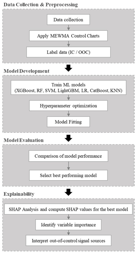
The methodological steps of this study are presented in the flowchart shown in Figure 1. First, production process data were collected, and each observation was labeled as IC or OOC based on MEWMA control charts. Then, classification models were developed using XGBoost, Random Forest, SVM, LightGBM, Logistic Regression, CatBoost, and KNN. XGBoost hyperparameters were optimized using stratified cross-validation, whereas the remaining classifiers were evaluated using the predefined configurations reported in Section 3.3. The models’ performance was compared using confusion matrix-based metrics. The model selected based on balanced and operationally suitable performance was then analyzed using SHAP. SHAP analysis explained the model’s decisions both globally and locally, identifying which variables contribute most to the OOC classification. Thus, by combining MEWMA’s sensitivity to small shifts with SHAP’s interpretability, a holistic approach was developed for detecting OOC signals and interpreting the model-based variable contribution patterns associated with these decisions.

3.1. Data Collection and Preprocessing

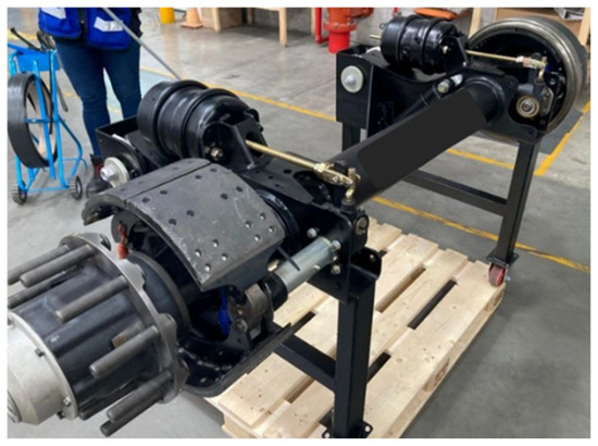
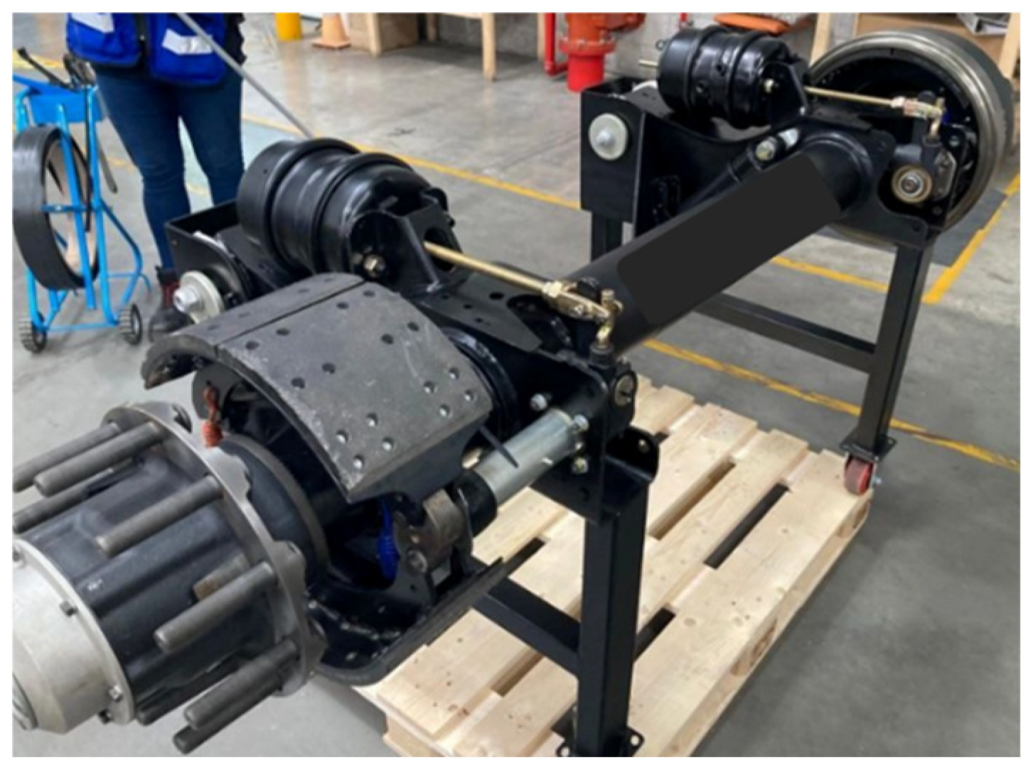
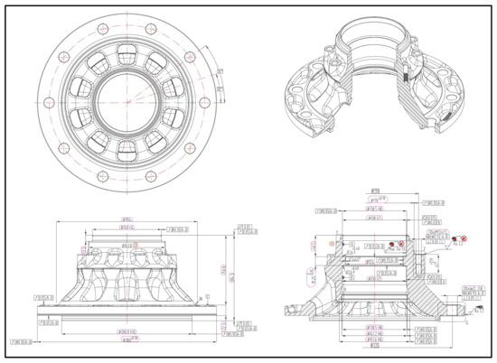
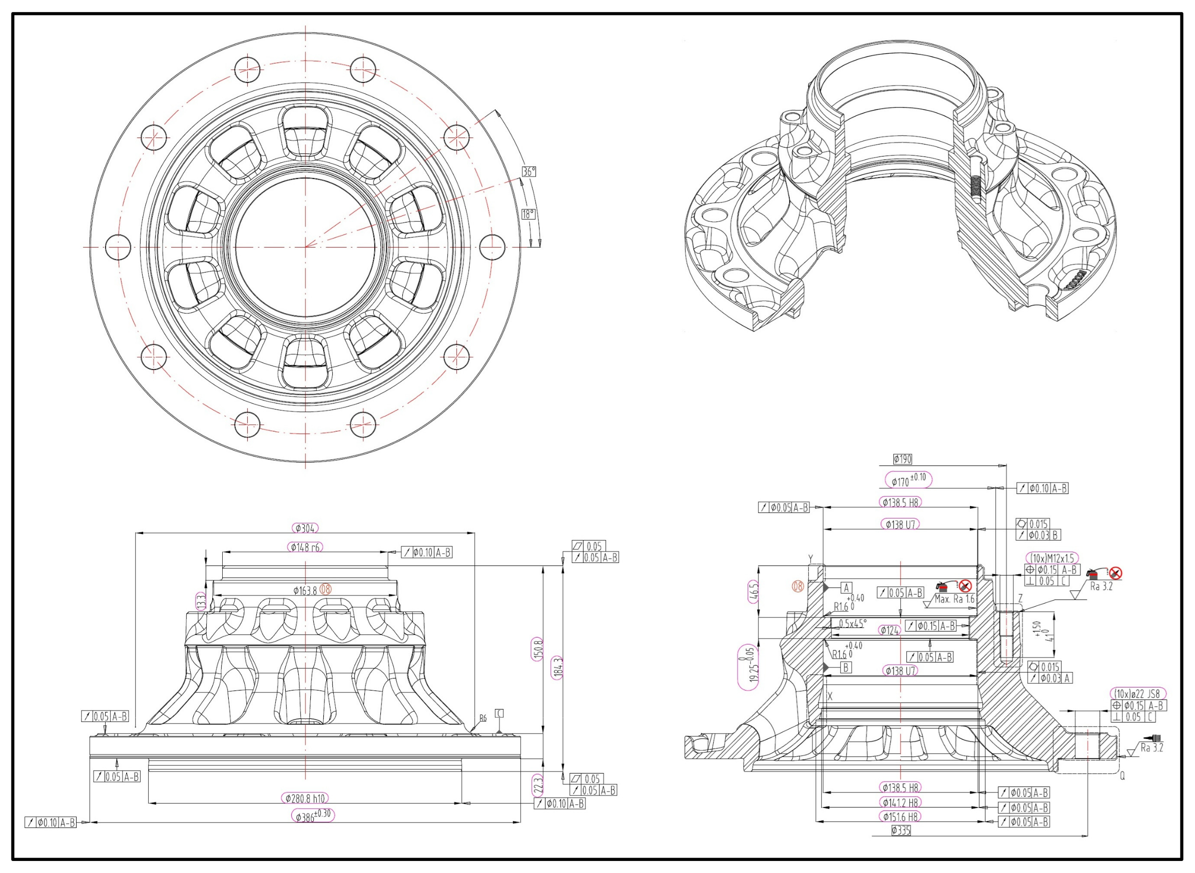
The dataset used in this study consists of 1000 multivariate observations from the production process of a hub, a critical safety component in the automotive industry. Each observation includes three-dimensional quality characteristics critical to the part’s functional performance: Diameter, Height, and Thickness. The product under investigation is manufactured from raw hub spheroidal cast iron (GGG45) material from the casting process. In its final form, this component is a high-safety-class automotive component mounted on the vehicle axle, together with the bearing, and provides load transfer to the wheel-rim system (Figure 2). The technical drawing of the part and the regions where these three-dimensional characteristics are located are shown in Figure 3.

The part under investigation is a functionally critical intermediate component in the automotive system. Dimensional deviations may lead to significant quality and safety concerns, including excessive tightness or looseness during assembly, bearing problems, friction-induced heating, degraded braking performance, and decreased final product reliability. Therefore, early detection of small dimensional deviations in internal production processes is crucial. However, this component is not the final product that directly reaches the end user; it undergoes subsequent assembly, inspection, and quality assurance steps. In this context, both Type I and Type II errors may have significant process consequences. A Type I error, in which an IC process is mistakenly classified as OOC, may lead to unnecessary downtime, additional measurement activities, and rework costs. Conversely, a Type II error, in which a true OOC signal is overlooked, may allow a defective part to proceed to subsequent production or assembly stages. Therefore, reliable detection of small process deviations is important in terms of both cost and quality/safety.

Before training the ML models, the dataset was split into two parts using a stratified random split, with 80% for training and 20% for testing. This ensures that the class distribution of IC and OOC labels is preserved in both subsets. Data preprocessing steps were carried out as follows:

• The dataset was verified to be free of missing observations, and the measurement records were pre-reviewed for data quality; this review revealed no records indicating missing data or measurement/data entry errors.
• Although MEWMA analysis is theoretically based on the assumption of multivariate normality, data transformation was not applied because MEWMA is relatively robust to moderate deviations from normality, as reported by Stoumbos and Sullivan [13].
• For MEWMA-based labeling, the original dimensional measurements were used to preserve the natural covariance structure of the process. Z-score standardization was applied only in the ML stage for scale-sensitive models, namely KNN, SVM, and Logistic Regression. Tree-based models, including XGBoost, Random Forest, LightGBM, and CatBoost, were trained using the original feature scale, since their splitting mechanisms are not directly affected by feature scaling. Standardization was particularly necessary for KNN because distance-based classification may otherwise be dominated by variables with larger numerical ranges.

3.2. MEWMA Chart and Labeling OOC Signals

The MEWMA control chart was selected because of its sensitivity to small and persistent shifts in correlated quality characteristics. In the chart design, the ARL value of 370, commonly used in the SPC literature, was adopted. This value indicates that approximately 0.27% false alarms will be generated (α = 0.0027) when the process is IC [1]. The smoothing parameter λ = 0.20 used in the MEWMA statistic increases the sensitivity to small and persistent shifts while avoiding overreaction to random noise in the process [13].

The dataset was divided into two phases, Phase I and Phase II, in accordance with the two-phase monitoring approach commonly used in the SPC literature. This approach aims to reliably estimate in-control (IC) process parameters and then evaluate process monitoring performance using the obtained parameters. A total of 250 observations were used in Phase I to estimate the IC process parameters, while the remaining observations were used in Phase II for process monitoring and OOC signal detection. The estimated IC mean vector and covariance matrix obtained from Phase I are given as follows:

$$\mu = \left[134.208, 161.423, 27.835\right] \mathrm{a}\mathrm{n}\mathrm{d} \Sigma =\left[\begin{array}{ccc}8.1494& -0.4366& -0.1723\\ -0.4366& 0.9297& 0.3520\\ -0.1723& 0.3520& 0.4123\end{array}\right].$$

Although the MEWMA chart is theoretically derived under the assumption of multivariate normality, previous studies have shown that it remains robust under moderate deviations from normality [13]. Therefore, no transformation was applied to preserve the original data structure.

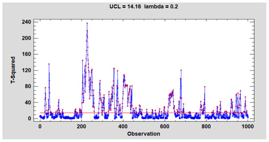
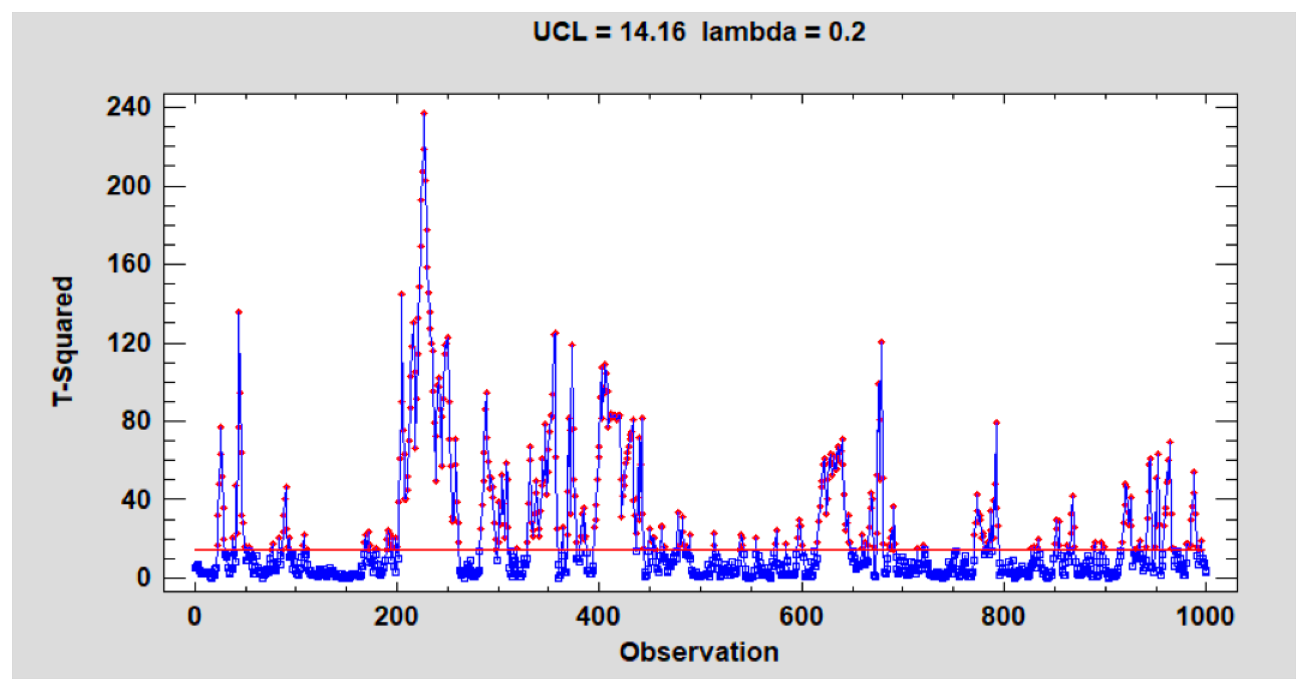
A MEWMA chart in Figure 4 was created taking into account the covariance structure between the three variables, and the UCL value of 14.1562 was calculated using the standard MEWMA design procedure based on p = 3 quality characteristics, λ = 0.20, and the target in-control ARL₀ (Average Run Length) = 370, rather than being empirically fitted from the Phase II data. A total of 400 observations exceeding the defined control limit were considered OOC signals in the process. Each of the 1000 observations in the dataset was labeled according to its position on the MEWMA chart: 600 observations in the IC state were coded as “0”, and 400 observations generating OOC signals were coded as “1”. This resulting binary-label structure enables the transformation of statistical monitoring outputs into a supervised learning problem and was used as the target variable in ML classification models to be developed in the next stage.

3.3. Classification with ML Algorithms

Seven ML algorithms (XGBoost, RF, SVM, LightGBM, LR, CatBoost, and KNN) were compared to model the binary labels (0 = IC, 1 = OOC) obtained from the MEWMA control chart. These models were preferred because they represent both linear and nonlinear decision boundaries, adapt to tabular data structures, and have been widely reported in the literature for their classification performance.

All models were evaluated using the same stratified train–test split, with 80% of the observations used for training and 20% for testing; the split was generated with random_state = 42. Z-score standardization was applied only to the scale-sensitive models, namely KNN, SVM, and Logistic Regression, while the tree-based models were trained using the original feature scale.

XGBoost was optimized using a three-fold stratified grid search with average precision (AUC–PR) as the selection criterion. The remaining classifiers were trained using the predefined configurations reported in

Table 1. Hyperparameter search ranges, final configurations, class weighting, and random seeds.

Model	Search Range/Fixed Configuration	Final Configuration	Class Weighting	Seed
XGBoost	n_estimators ∈ {100, 200};	100;	scale_pos_weight = 1.50	42
	max_depth ∈ {3,4,5};	3;
	learning_rate ∈ {0.1, 0.2};	0.1;
	subsample ∈ {0.8, 1.0};	0.8;
	min_child_weight ∈ {1, 3, 5};	1;
	gamma ∈ {0, 0.1, 0.2}	0.2
Random Forest	n_estimators; max_depth	200; 5	balanced	42
SVM	kernel; C; gamma;	RBF kernel; 1.0; scale	balanced	42
LightGBM	n_estimators; learning rate; max depth;	300; 0.05; 5	balanced	42
LR	C; solver; maximum iterations	1.0; liblinear; 1000	balanced	42
CatBoost	iterations; depth; learning rate	300; 5; 0.05	scale_pos_weight = 1.50	42
KNN	k; weighting; metric; p	5; distance; Minkowski; p = 2 (Euclidean)	None	N/A

. All stochastic procedures used a random seed of 42, whereas KNN is deterministic for a fixed dataset and parameter configuration.

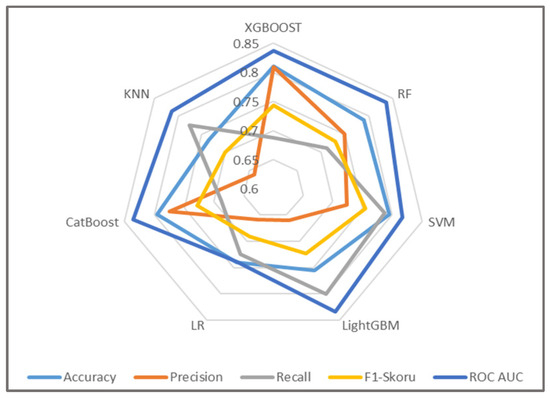
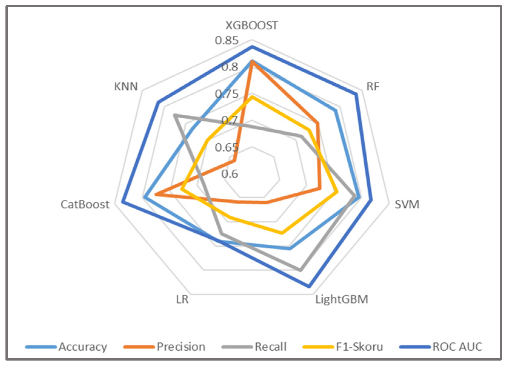
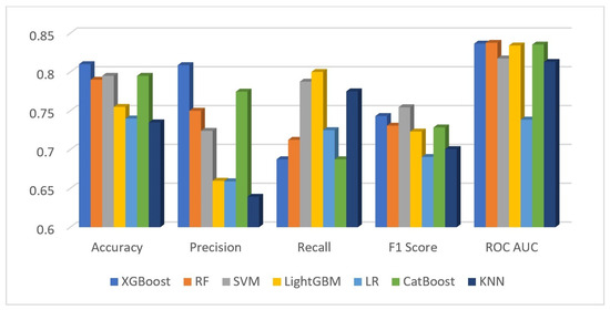
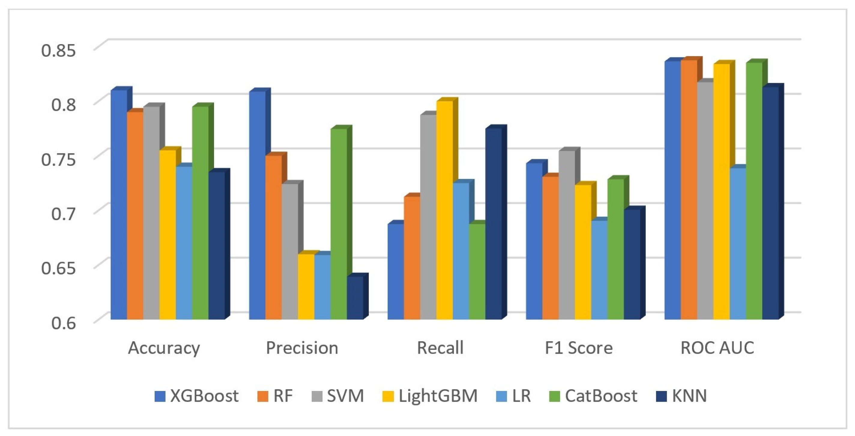
Accuracy, Precision, Recall, F1-score, and ROC AUC were used as evaluation metrics. In the calculation of these values, True Positive (TP), True Negative (TN), False Positive (FP), and False Negative (FN) are considered. The confusion matrix in $\left[\begin{array}{cc}TN& FP\\ FN& TP\end{array}\right]$ format was used. The performance comparison of the models is given in

Table 2. Performance comparison of ML algorithms.

Performance Metrics	XGBoost	RF	SVM	LightGBM	LR	CatBoost	KNN
Accuracy	0.8100	0.7900	0.7950	0.7550	0.7400	0.7950	0.7350
Precision	0.8088	0.7500	0.7241	0.6598	0.6591	0.7746	0.6392
Recall	0.6875	0.7125	0.7875	0.8000	0.7250	0.6875	0.7750
F1 Score	0.7432	0.7308	0.7545	0.7232	0.6905	0.7285	0.7006
ROC AUC	0.8365	0.8375	0.8174	0.8341	0.7386	0.8353	0.8129
Confusion Matrix	$\left[\begin{array}{cc}107& 13\\ 25& 55\end{array}\right]$	$\left[\begin{array}{cc}101& 19\\ 23& 57\end{array}\right]$	$\left[\begin{array}{cc}96& 24\\ 17& 63\end{array}\right]$	$\left[\begin{array}{cc}87& 33\\ 16& 64\end{array}\right]$	$\left[\begin{array}{cc}90& 30\\ 22& 58\end{array}\right]$	$\left[\begin{array}{cc}104& 16\\ 25& 55\end{array}\right]$	$\left[\begin{array}{cc}85& 35\\ 18& 62\end{array}\right]$

, the radar chart of the metrics in Figure 5, and the bar chart in Figure 6.

Since the part under investigation is a functionally critical intermediate production component in the automotive system, both Type I and Type II errors must be considered during process monitoring. Therefore, the classification models were compared not only in terms of overall accuracy, but also by considering their ability to capture the OOC class (Recall) and their tendency to generate false alarms (Precision). Although the LightGBM and SVM models achieved higher Recall values for the OOC class, their lower Precision values indicate a greater tendency to generate false alarms. In contrast, the XGBoost model achieved the highest Accuracy (81.00%) and Precision (80.88%) and demonstrated balanced and competitive performance in terms of F1-score and ROC-AUC. Therefore, XGBoost was evaluated as a more suitable decision-support model for this application, as it provided a better trade-off between Type I and Type II errors. For this reason, SHAP analysis was conducted using the XGBoost model to examine the variable contributions associated with IC/OOC classification decisions.

To verify whether the apparent performance advantage of XGBoost is statistically meaningful rather than incidental, two complementary hypothesis tests were conducted. First, a pairwise McNemar exact test was applied to compare the classification performance of XGBoost with other models on a test set of 200 common observations; the null hypothesis (H0) was tested, based on the assumption that there is no significant difference in classification performance between XGBoost and the model being compared. As shown in

Table 3. McNemar’s exact test: XGBoost versus each competing model (common test set).

Comparison	p-Value	Significant (α = 0.05)
XGBoost vs. CatBoost	0.508	No
XGBoost vs. SVM	0.728	No
XGBoost vs. RF	0.503	No
XGBoost vs. LightGBM	0.061	No
XGBoost vs. LR	0.029	Yes
XGBoost vs. KNN	0.028	Yes

, XGBoost did not differ significantly from the other strong models, including CatBoost (p = 0.508), SVM (p = 0.728), RF (p = 0.503), and LightGBM (p = 0.061). However, XGBoost outperformed the baseline linear and instance-based models, namely LR (p = 0.029) and KNN (p = 0.028), at the 5% significance level. Second, a Friedman test was performed over repeated stratified cross-validation using the F1 score of the OOC class as the performance metric. The Friedman test indicated a statistically significant difference among the models (χ² = 81.85, p < 0.001), confirming the presence of overall differences among the seven models. The subsequent Nemenyi post hoc test (

Table 4. Nemenyi post hoc p-values for XGBoost (Friedman test: χ² = 81.85, p < 0.001).

	CatBoost	SVM	RF	LightGBM	LR	KNN
XGBoost	0.996	1.000	0.376	0.951	<0.001	<0.001

) reproduced the same pattern: XGBoost did not differ significantly from CatBoost (p = 0.996), SVM (p = 1.000), RF (p = 0.376), or LightGBM (p = 0.951), but differed significantly from LR and KNN (p < 0.001 for both). These findings indicate that XGBoost is statistically comparable to the other ensemble and kernel-based models and is significantly better only than the linear and instance-based baselines. Accordingly, XGBoost was selected for the explainability analysis not because of a statistically significant improvement in accuracy over the other strong models, but because it exhibited a more balanced Type I/Type II error trade-off and is natively compatible with the exact SHAP explainer employed in the next stage.

Although the ML models are trained on MEWMA-generated labels, they enable nonlinear decision boundary learning and provide a scalable classification framework beyond traditional control chart interpretation.

3.4. SHAP Explainability Analysis

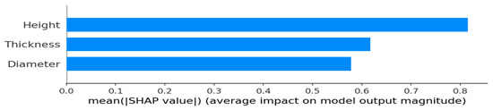
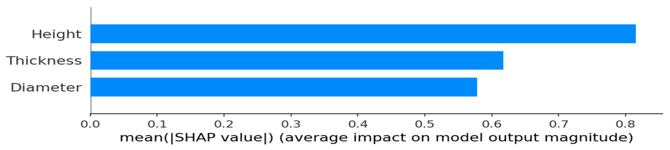
In this study, the XGBoost model’s classification outputs were examined for explainability using the SHAP method. First, a global significance analysis of SHAP was performed, and the average effect size of each variable on the model was evaluated across the entire data set. Figure 7 shows the global importance plot of the three metric variables sorted by their mean absolute SHAP values.

According to the analysis results, Height is the most dominant variable in the model’s decision mechanism, with an average SHAP value of approximately 0.85. This value shows that changes in Height produce a larger marginal contribution to the model’s OOC predictions than other variables. The Thickness variable follows Height with an average SHAP value of ~0.62 and Diameter with an average SHAP value of ~0.58. The lengths in the bar charts represent the magnitude of the average effect of the relevant feature on the probability of the model’s output; therefore, the order of the bar lengths indicates the relative importance of the variables in the model. These results reveal that the XGBoost model shows higher sensitivity to shifts, especially in Height and Thickness variables, when parsing multivariate signals marked by MEWMA. These findings indicate that SHAP provides a consistent and interpretable model-based explanation of variable contributions associated with MEWMA-generated OOC classifications.

The global SHAP analysis quantitatively reveals which variables contribute most to the OOC classification decisions of the XGBoost model for observations labeled as OOC by MEWMA. That is, the calculated SHAP values enabled the identification of the dominant contributing variable(s) for each OOC signal. Accordingly, the analysis for 400 OOC observations shows that the dominant contributing variable to the model’s OOC classification decisions was Height (42.0% [168 observations]), followed by Thickness (29.8% [119 observations]), and Diameter (28.2% [113 observations]). In summary, SHAP analysis not only revealed which variables the model predominantly used but also provided a model-based interpretation of variable contributions associated with MEWMA-generated OOC signals from a variable-based, quantitative perspective.

Table 5. SHAP contribution analysis of OOC observations.

Case (Status = 1)	Property Values (Diameter, Height, Thickness)	Main Contributing Feature (Contribution of %)	Second Contribution (Contribution of %)
#23	134.20, 163.77, 27.03	Height—66.1%	Diameter—30.5%
#94	142.8, 161.89, 28.23	Diameter—69.55%	Thickness—23.76%
#241	132.46, 162.01, 26.3	Thickness—82.84%	Diameter—12.68%

summarizes the percentage contributions of the most influential variables for the three representative OOC signals. Accordingly, the model highlights which variable contributes most to the OOC classification decision for each observation labeled as OOC by MEWMA. For example, the dominant contributing factor in the model’s decision in observation number 241 is that the Thickness variable is at a level of 26.3 mm, which is lower than the typical thickness values in the training data. The fact that 82.84% of the total SHAP contribution comes from this variable indicates that this decrease in thickness is the primary factor explaining the model’s OOC prediction. Similarly, when the model’s decision structure is examined in observation 23, it is seen that the primary variable explaining the model’s OOC classification decision is Height. In this observation, the model interprets the increase in Height to 163.77 as unusually high compared to typical height values in the training data and accounts for 66.1% of the total SHAP contribution alone.

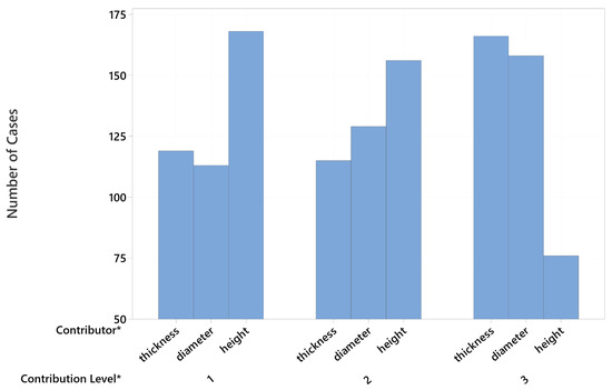
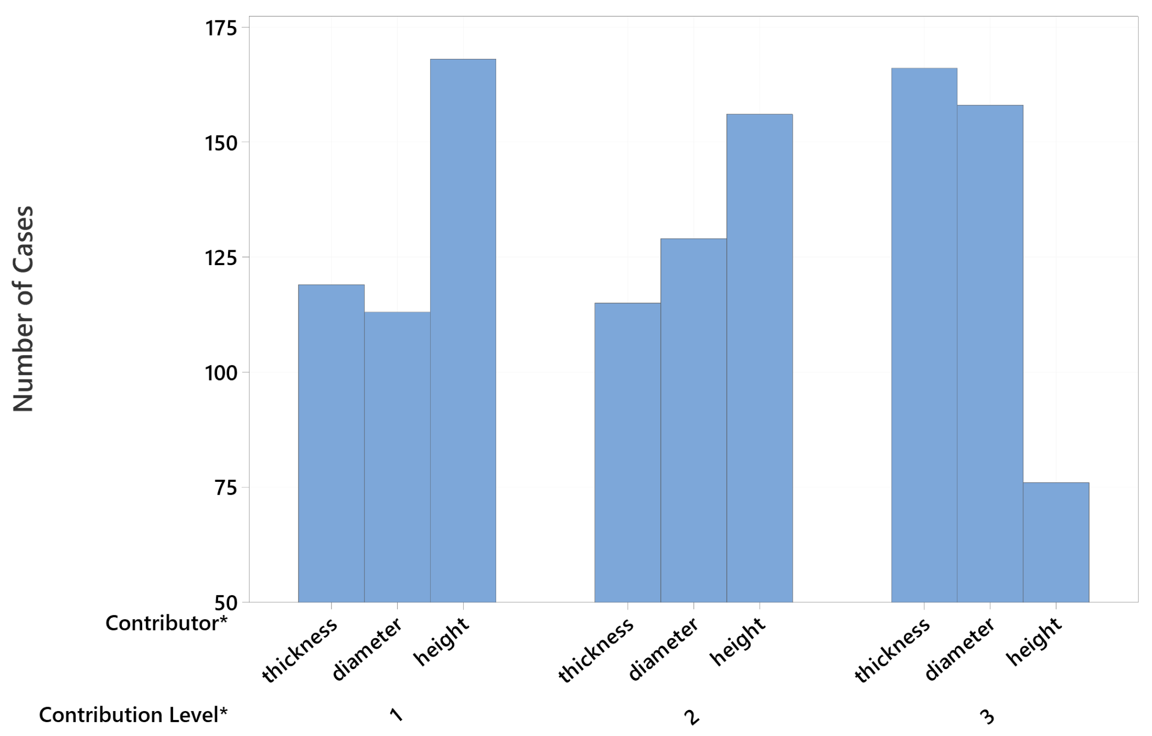
These findings demonstrate that the SHAP method not only clarifies the variable contributions associated with individual OOC classification decisions but also reveals systematic patterns in variable contributions across all observations labeled as OOC by MEWMA. The contribution distribution plot in Figure 8 quantitatively compares how often each variable appears as a primary, secondary, or tertiary contributing factor, according to its contribution order, across 400 observations labeled as OOC by MEWMA.

As shown in the graph, Height appears most frequently as the primary contributing variable, Thickness plays a role at the secondary contribution level, and Diameter, while mostly at the tertiary level, provides primary contributions in some cases. This distribution, consistent with the global SHAP ranking, shows that height and thickness are, in particular, the most influential variables in the model’s decision of OOC classification. Therefore, SHAP analysis highlights, in an interpretable manner, which variables are most strongly associated with the model’s OOC classification decisions detected by MEWMA, both at the local level (based on individual observations) and at the global level (across the overall distribution within 400 observations labeled as OOC by MEWMA). These quantitative results may provide a directly applicable decision-support mechanism for both process engineers and quality management teams by showing which metric characteristics the process is most sensitive to.

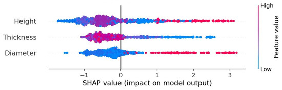
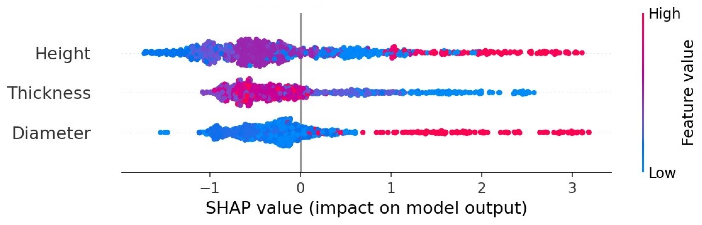
Based on these general findings, a beeswarm plot was used to examine the distribution of SHAP values in more detail, and the effect of each variable on the model output was visually analyzed for both direction and magnitude. In the beeswarm plot presented in Figure 9, each point represents an observation, while the horizontal values indicate the calculated SHAP value for that observation. Positive SHAP values increase the model’s tendency to classify the observation as OOC, while negative values support controlled classification. The color scale indicates whether the feature value is high (red) or low (blue), providing additional insight into how variable values influence the OOC classification decisions.

When the graph is examined, it is seen that high values of the Height variable are predominantly concentrated in the positive SHAP region, indicating that above-normal height measurements push the model toward the OOC class. However, the fact that some low-height values also yield positive SHAP values indicates that both low and high extreme shifts in height pose a risk. For the Thickness variable, the concentration of low thickness values in the positive SHAP region shows that the model assigns stronger OOC-related contributions when the part is thinner than usual. High thickness values, on the other hand, are mainly in the negative region, contributing to the control status. For the Diameter variable, it is observed that high-diameter values are concentrated on the positive SHAP side, while low values are concentrated on the negative side; this finding indicates that parts with diameters larger than normal are more likely to exhibit an anomaly.

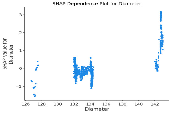
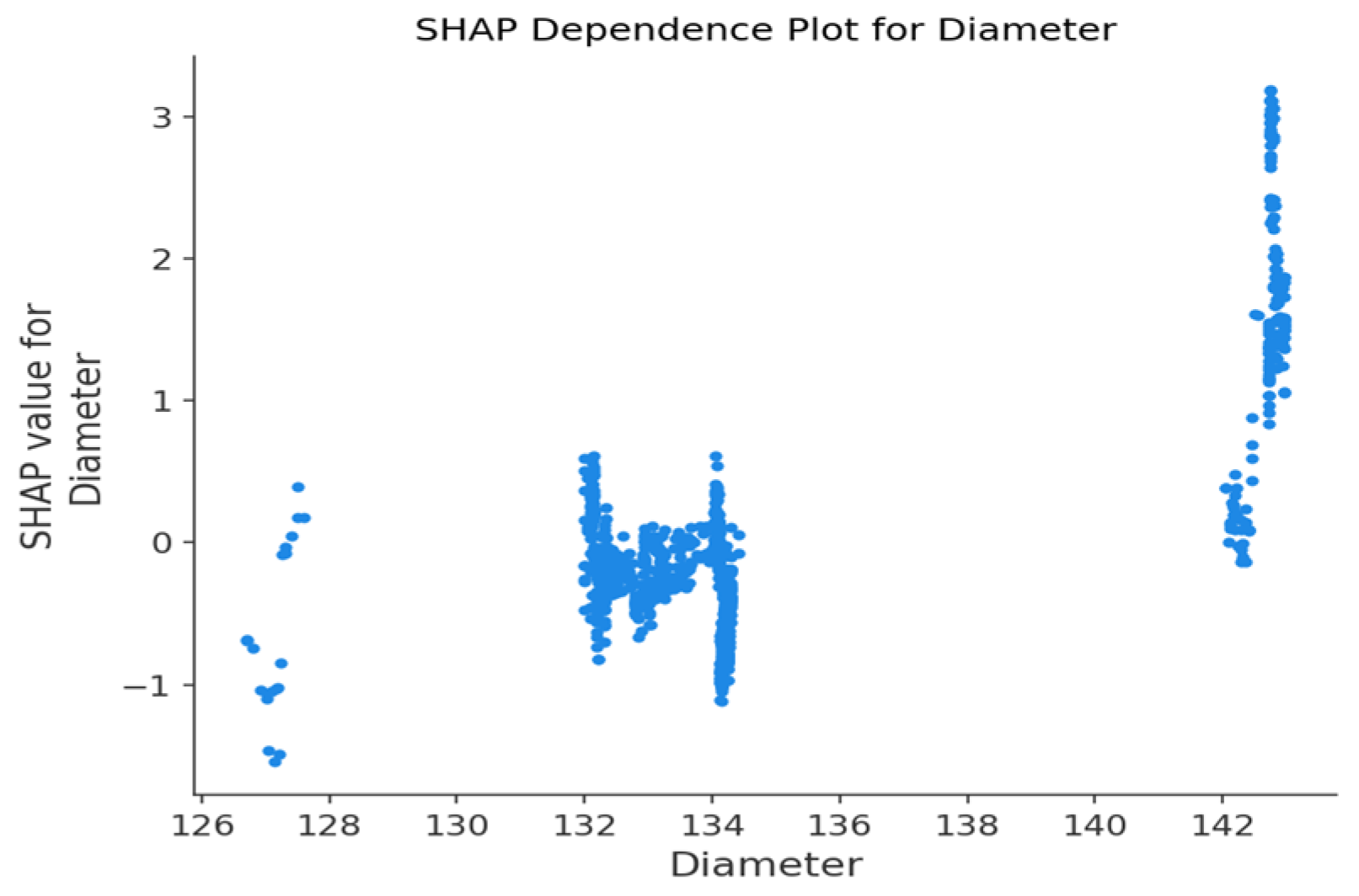
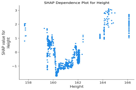
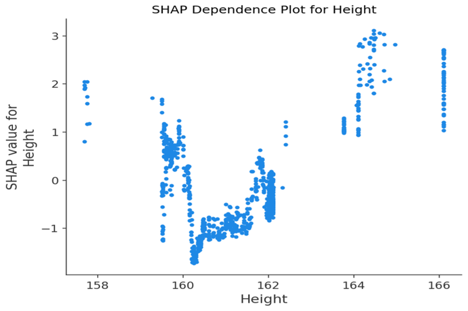
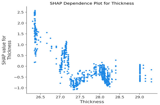
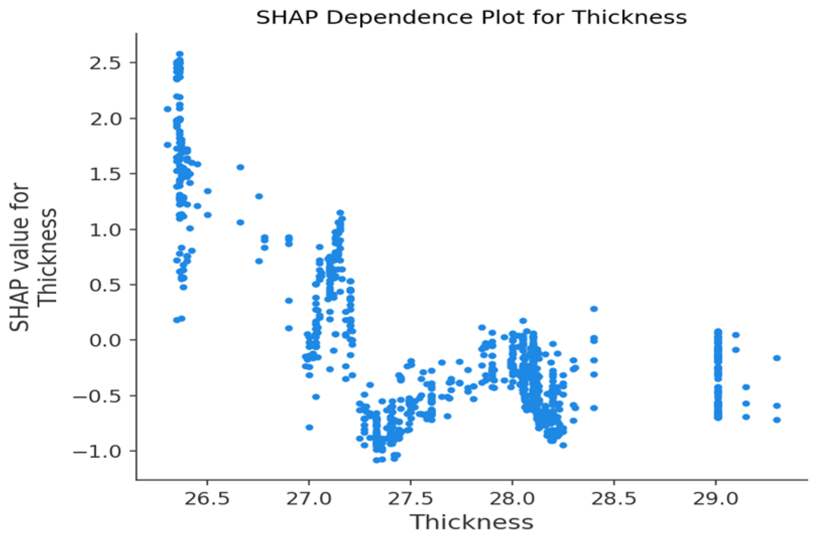
In general, the beeswarm analysis shows that the model is susceptible to anomalies, especially to low thickness values, high diameter values, and extreme height values (both low and high). Furthermore, by comprehensively revealing the effects of variable values on the model output, both in direction and distribution, it significantly contributes to understanding the model’s overall decision structure. In addition, dependency graphs were used to examine, within the scope of this study, the relationship between variable values and the SHAP effect in more detail, at the point level. Figure 10, Figure 11 and Figure 12 present the SHAP dependency graphs for the Diameter, Height, and Thickness variables, respectively, and show more directly how changes in each feature’s value are reflected in the model’s anomaly prediction.

The dependency graph for the Diameter variable shows that as the diameter increases, the SHAP value increases and the probability of anomalies increases significantly, especially at values above 140 mm. The dependency graph obtained for the Height variable shows that the SHAP effect increases positively at both low and high extreme values; this confirms that extreme shifts in height can cause anomalies. The dependency graph for the Thickness variable shows that the SHAP effect is strongly positive at low thickness values; as thickness increases, the model tends to prefer the controlled class.

These dependency graphs confirm the general trends observed in the beeswarm analysis for each variable and provide a precise, interpretable view that complements the SHAP analysis by detailing the functional form of each dimensional characteristic’s contribution to model prediction.

These results indicate that the XGBoost model shows higher sensitivity to shifts, particularly in Height and Thickness variables, when interpreting multivariate signals identified by MEWMA. This demonstrates that SHAP provides a strong diagnostic contribution by offering a model-based explanation of variable contributions to OOC classification decisions and by enhancing the model’s interpretability.

3.5. Computational Efficiency and Real-Time Applicability

In addition to predictive performance and interpretability, computational efficiency is an important requirement for the practical implementation of the proposed framework in real-time industrial monitoring environments. In the proposed structure, model training, hyperparameter optimization, and global SHAP analysis are performed offline. Therefore, these stages do not affect online monitoring latency. During online deployment, each incoming observation requires only three operations: updating the MEWMA statistic, obtaining the prediction from the trained XGBoost model, and, when diagnostic interpretation is required, computing local SHAP values for the corresponding observation.

To evaluate the real-time feasibility of the proposed framework, a time-tracking experiment was conducted on a computer equipped with a 2.8 GHz Intel Core i7-7700 CPU and 16 GB of RAM. The analyses were implemented in Python 3.11.5 using scikit-learn 1.3.0, XGBoost 3.0.5, LightGBM 4.6.0, CatBoost 1.2.8, SHAP 0.52.0, NumPy 1.24.3, and pandas 2.0.3. The processing time for a single observation was measured after model loading and warm-up runs. The results are presented in

Table 6. Single-observation processing time of the proposed framework.

Processing Step	Mean Time (s)	Standard Deviation (s)	Median (s)	95th Percentile (s)
MEWMA update	0.000055	0.000009	0.000055	0.00007
XGBoost prediction	0.010742	0.025676	0.002093	0.08734
SHAP explanation	0.084255	0.030924	0.096790	0.10032
Total processing time	0.095052	0.035659	0.099403	0.18292

.

The results show that the proposed framework processes a single observation in approximately 0.095 s on average, with a 95th percentile latency of approximately 0.183 s. Since the computationally intensive stages are conducted offline, the online computational cost remains limited. Moreover, SHAP can be triggered only for observations classified as OOC, rather than for all IC observations. This event-triggered interpretation strategy further reduces computational overhead and supports the applicability of the proposed framework in real-time or near-real-time industrial process monitoring.

4. Results and Discussion

This study investigates the detection and interpretation of multivariate OOC signals in the manufacturing process, MEWMA control charts, machine learning-based classification models, and the SHAP explainability method. This integrated approach not only identifies MEWMA-based OOC signals but also provides a quantitative, interpretable understanding of the variable contributions to MEWMA-based OOC classification decisions, extending traditional control chart analysis into a data-driven, explainable monitoring approach.

In the application section using MEWMA control charts, a total of 400 OOC signals were generated from 1000 observations, clearly demonstrating the process’s sensitivity to slight shifts. Various ML algorithms were evaluated to model the IC/OOC labels generated by MEWMA; the results were compared using Accuracy, Precision, Recall, F1-score, and ROC AUC metrics. The comparison results showed that XGBoost provided the most balanced overall performance in terms of Accuracy, Precision, F1-score, ROC-AUC, and the Type I/Type II error trade-off. The model’s confusion matrix results indicated that both Type I and Type II errors were within acceptable ranges; therefore, XGBoost was selected for the explainability analysis.

The main contribution of this study is the interpretation of multivariate MEWMA signals on a variable-by-variable basis using the SHAP method. Although SHAP is widely applied in various fields, its use in interpreting machine learning models trained on multivariate control chart outputs has been limited in the literature. Therefore, this study contributes to the growing intersection of SPC and XAI.

The global significance analysis of SHAP showed that the Height variable is the most dominant feature in explaining the model’s OOC classification decisions, followed by the Thickness and Diameter variables. Quantitative analyses revealed that Height was the primary determinant in 42% of 400 OOC observations, Thickness in 29.8%, and Diameter in 28.2%. These results indicate that the process is susceptible to changes in height and thickness measurements. A more detailed examination of SHAP value distributions enabled a more holistic understanding of the model-based OOC classification pattern in the process. The findings show that the model’s tendency to exhibit anomalies increases significantly at low thickness values, high diameter values, and at both low and high height endpoints. This suggests that OOC signals are associated with multidimensional patterns formed by the combination of variables rather than with the extreme value of a single variable. Local SHAP analyses also supported these findings, demonstrating that individual OOC classification decisions were influenced by distinct combinations of variables and highlighting the complex nature of multivariate variation.

When considered together with these findings, the study points to three key conclusions. First, MEWMA is an effective monitoring tool that can detect small, cumulative shifts at an early stage. Second, the XGBoost model learned the MEWMA-generated classification patterns and provided a scalable decision-support layer for reproducing and explaining MEWMA-based IC/OOC decisions. Third, and most importantly, the SHAP method quantitatively explained variable contributions to OOC classification decisions, enabling interpretation of the control chart output at the operator and engineer levels. This feature helps overcome the interpretability limitation of multivariate control charts, which states that “it is not possible to know which variable is causing the signal.” The study’s findings are directly applicable to production engineering and quality management. Variable contributions obtained from SHAP analysis highlight critical metric parameters affecting process stability and indicate which variables are most strongly associated with OOC classification decisions. In this way, process behavior can be better understood, and situations that may disrupt process stability can be detected at an early stage. In addition, the proposed approach provides a foundation for the development of interpretable monitoring structures that can not only generate alarms but also explain the variable contributions underlying model decisions in real-time process monitoring systems. The additional computational efficiency analysis also showed that the proposed framework can process a single observation in approximately 0.095 s on average, indicating its feasibility for real-time or near-real-time process monitoring when training and global explanation stages are performed offline. This study offers potential applications across various fields for future research. Integration of different multivariate control charts, such as MEWMA, Hotelling T², and MCUSUM with SHAP and similar explainable artificial intelligence methods; comparison of the performance of methods such as SHAP, LIME, or Integrated Gradients on larger datasets; application of dynamic SHAP approaches in time-dependent processes; and development of SHAP-based decomposition systems in real-time production environments are potential future studies.

5. Conclusions and Limitations

This study integrates MEWMA control charts, ML classification models, and a SHAP-based explainability approach to both detect and explain small and cumulative shifts at the variable level in a multivariate production process. In the first stage, MEWMA successfully identified OOC observations in the process thanks to its sensitivity to small changes. Then, the goal was to learn the MEWMA-generated classification structure using various ML algorithms; the results showed that the XGBoost model provided a balanced classification profile with the highest Accuracy and Precision among the evaluated models, although its superiority over other tree-based ensemble models was not statistically significant according to McNemar’s test. Finally, SHAP analysis explained the model’s decision-making mechanism at the variable level, quantitatively revealing which features contribute most to OOC classification decisions at both global and local scales.

The findings show that the height variable is the most dominant factor in explaining the model’s OOC classification decisions; thickness and diameter variables also make substantial contributions in different combinations. Thus, the study provides an explainable solution that supports not only the “signal generation” function of MEWMA but also the processes of interpreting these signals through variable contributions. In this context, the proposed approach provides an interpretable and practical tool for determining the contributions of variable(s) associated with OOC signals in industrial process monitoring. The per-observation timing experiment also indicated that the proposed framework can be implemented in real-time or near-real-time monitoring settings without imposing a substantial computational burden.

This study contributes to the literature by integrating SHAP-based explainability with MEWMA-based multivariate process monitoring. The integration of statistical monitoring and explainable machine learning provides an interpretable approach to multivariate process-monitoring interpretation.

The limitations of the study are as follows: Firstly, the dataset was obtained from a single production line, containing only three metric quality characteristics; therefore, caution should be exercised when generalizing the results to different product types or processes with larger datasets. Secondly, since SHAP analysis is a model-dependent explainability approach, the interpretations presented are limited to the decision structure of the XGBoost model. Variable importance rankings or contribution magnitudes may differ across ML algorithms. Thirdly, although the original SPC data have an inherent sequential structure, the machine learning stage in this study was formulated as a classification task and did not explicitly model temporal dependencies among observations. Autocorrelation structures and dynamic process behaviors that may occur in real production environments are outside the scope of this study. Despite these limitations, the study demonstrates the potential of combining MEWMA-based monitoring with explainable machine learning for interpretable multivariate process analysis. Future studies are proposed to investigate processes involving higher data volumes, to compare the proposed SHAP-based explanation framework with classical MEWMA contribution and decomposition methods in terms of diagnostic accuracy, computational efficiency, and interpretability, to integrate different control chart types with SHAP and other XAI approaches, to develop dynamic models that consider time-series structures, and to design real-time decomposition systems.

References

- Montgomery, D.C. Introduction to Statistical Quality Control; John Wiley & Sons: New York, NY, USA, 2020. [Google Scholar]
- Yeganeh, A.; Johannssen, A.; Chukhrova, N. The partitioning ensemble control chart for on-line monitoring of high-dimensional image-based quality characteristics. Eng. Appl. Artif. Intell. 2024, 127, 107282. [Google Scholar] [CrossRef] [Scilit]
- Kazmi, M.W.; Noor-ul-Amin, M. Integrating machine learning based EWMA control charts for multivariate process monitoring. Comput. Ind. Eng. 2025, 204, 111131. [Google Scholar] [CrossRef] [Scilit]
- Weix, D.; Cath, T.Y.; Hering, A.S. Monitoring covariance in multivariate time series: Comparing machine learning and statistical approaches. Qual. Reliab. Eng. Int. 2024, 40, 2822–2840. [Google Scholar] [CrossRef] [Scilit]
- Sabahno, H.; Amiri, A. New statistical and machine learning based control charts with variable parameters for monitoring generalized linear model profiles. Comput. Ind. Eng. 2023, 184, 109562. [Google Scholar] [CrossRef] [Scilit]
- Yao, W.; Li, D.; Gao, L. Fault detection and diagnosis using tree-based ensemble learning methods and multivariate control charts for centrifugal chillers. J. Build. Eng. 2022, 51, 104243. [Google Scholar] [CrossRef] [Scilit]
- Bersimis, S.; Sgora, A.; Psarakis, S. Methods for interpreting the out-of-control signal of multivariate control charts: A comparison study. Qual. Reliab. Eng. Int. 2017, 33, 2295–2326. [Google Scholar] [CrossRef] [Scilit]
- Ali, S.; Abuhmed, T.; El-Sappagh, S.; Muhammad, K.; Alonso-Moral, J.M.; Confalonieri, R.; Guidotti, R.; Del Ser, J.; Díaz-Rodríguez, N.; Herrera, F. Explainable artificial intelligence (XAI): What we know and what is left to attain trustworthy artificial intelligence. Inf. Fusion 2023, 99, 101805. [Google Scholar] [CrossRef] [Scilit]
- Lundberg, S.M.; Lee, S.-I. A unified approach to interpreting model predictions. In Advances in Neural Information Processing Systems; Curran Associates: Red Hook, NY, USA, 2017; pp. 4765–4774. [Google Scholar]
- Lundberg, S.M.; Erion, G.; Chen, H.; DeGrave, A.; Prutkin, J.M.; Nair, B.; Katz, R.; Himmelfarb, J.; Bansal, N.; Lee, S.-I. From local explanations to global understanding with explainable AI for trees. Nat. Mach. Intell. 2020, 2, 56–67. [Google Scholar] [CrossRef] [Scilit] [PubMed]
- Lowry, C.A.; Woodall, W.H.; Champ, C.W.; Rigdon, S.E. A multivariate exponentially weighted moving average control chart. Technometrics 1992, 34, 46–53. [Google Scholar] [CrossRef] [Scilit]
- Bersimis, S.; Psarakis, S.; Panaretos, J. Multivariate statistical process control charts: An overview. Qual. Reliab. Eng. Int. 2007, 23, 517–543. [Google Scholar] [CrossRef] [Scilit]
- Stoumbos, Z.G.; Sullivan, J.H. Robustness to non-normality of the multivariate EWMA control chart. J. Qual. Technol. 2002, 34, 260–276. [Google Scholar] [CrossRef] [Scilit]
- Woodall, W.H. Controversies and contradictions in statistical process control. J. Qual. Technol. 2000, 32, 341–350. [Google Scholar] [CrossRef] [Scilit]
- Mason, R.L.; Tracy, N.D.; Young, J.C. Decomposition of T2 for multivariate control chart interpretation. J. Qual. Technol. 1995, 27, 99–108. [Google Scholar] [CrossRef] [Scilit]
- Johannssen, A.; Qiu, P.; Yeganeh, A.; Chukhrova, N. Explainable AI for trustworthy intelligent process monitoring. Comput. Ind. Eng. 2025, 209, 111407. [Google Scholar] [CrossRef] [Scilit]
- Chen, T.; Guestrin, C. XGBoost: A scalable tree boosting system. In Proceedings of the 22nd ACM SIGKDD International Conference on Knowledge Discovery and Data Mining; ACM: New York, NY, USA, 2016; pp. 785–794. [Google Scholar] [CrossRef] [Scilit]
- Zhao, Z.; Duan, W.; Cai, G.; Wu, M.; Liu, S. CPT-based fully probabilistic seismic liquefaction potential assessment to reduce uncertainty: Integrating XGBoost algorithm with Bayesian theorem. Comput. Geotech. 2022, 149, 104868. [Google Scholar] [CrossRef] [Scilit]
- Khan, A.A.; Chaudhari, O.; Chandra, R. A review of ensemble learning and data augmentation models for class imbalanced problems: Combination, implementation and evaluation. Expert Syst. Appl. 2024, 244, 122778. [Google Scholar] [CrossRef] [Scilit]
- Nijman, S.W.J.; Leeuwenberg, A.M.; Beekers, I.; Verkouter, I.; Jacobs, J.J.L.; Bots, M.L.; Asselbergs, F.W.; Moons, K.G.M.; Debray, T.P.A. Missing data is poorly handled and reported in prediction model studies using machine learning: A literature review. J. Clin. Epidemiol. 2022, 142, 218–229. [Google Scholar] [CrossRef] [Scilit] [PubMed]
- Breiman, L. Random forests. Mach. Learn. 2001, 45, 5–32. [Google Scholar] [CrossRef] [Scilit]
- Belgiu, M.; Dragut, L. Random forest in remote sensing: A review of applications and future directions. ISPRS J. Photogramm. Remote Sens. 2016, 114, 24–31. [Google Scholar] [CrossRef] [Scilit]
- Cortes, C.; Vapnik, V. Support-vector networks. Mach. Learn. 1995, 20, 273–297. [Google Scholar] [CrossRef] [Scilit]
- Oliveira, R.M.A.; Sant’Anna, Â.M.O.; da Silva, P.H.F. Explainable machine learning models for defects detection in industrial processes. Comput. Ind. Eng. 2024, 192, 110214. [Google Scholar] [CrossRef] [Scilit]
- Hastie, T.; Tibshirani, R.; Friedman, J. The Elements of Statistical Learning; Springer: New York, NY, USA, 2009. [Google Scholar]
- Cervantes, J.; Garcia-Lamont, F.; Rodríguez-Mazahua, L.; Lopez, A. A comprehensive survey on support vector machine classification: Applications, challenges and trends. Neurocomputing 2020, 408, 189–215. [Google Scholar] [CrossRef] [Scilit]
- Ke, G.; Meng, Q.; Finley, T.; Wang, T.; Chen, W.; Ma, W.; Ye, Q.; Liu, T.Y. LightGBM: A highly efficient gradient boosting decision tree. Adv. Neural Inf. Process. Syst. 2017, 30, 3149–3157. [Google Scholar]
- González, S.; García, S.; Del Ser, J.; Rokach, L.; Herrera, F. A practical tutorial on bagging and boosting based ensembles for machine learning. Inf. Fusion 2020, 64, 205–237. [Google Scholar] [CrossRef] [Scilit]
- Meng, Q.; Ke, G.; Wang, T.; Chen, W.; Ye, Q.; Ma, Z.M.; Liu, T.Y. A communication-efficient parallel algorithm for decision tree. Adv. Neural Inf. Process. Syst. 2016, 29, 1279–1287. [Google Scholar]
- Mienye, I.D.; Sun, Y.X. A survey of ensemble learning: Concepts, algorithms, applications, and prospects. IEEE Access 2022, 10, 99129–99149. [Google Scholar] [CrossRef] [Scilit]
- Nikolaou, D.; Ziakopoulos, A.; Dragomanovits, A.; Roussou, J.; Yannis, G. Comparing machine learning techniques for predictions of motorway segment crash risk level. Safety 2023, 9, 32. [Google Scholar] [CrossRef] [Scilit]
- Prokhorenkova, L.; Gusev, G.; Vorobev, A.; Dorogush, A.V.; Gulin, A. CatBoost: Unbiased boosting with categorical features. Adv. Neural Inf. Process. Syst. 2018, 31, 6639–6649. [Google Scholar]
- Ben Jabeur, S.; Gharib, C.; Mefteh-Wali, S.; Ben Arfi, W. CatBoost model and artificial intelligence techniques for corporate failure prediction. Technol. Forecast. Soc. Change 2021, 166, 120658. [Google Scholar] [CrossRef] [Scilit]
- Cover, T.; Hart, P. Nearest neighbor pattern classification. IEEE Trans. Inf. Theory 1967, 13, 21–27. [Google Scholar] [CrossRef] [Scilit]
- Yang, Y.; Liu, X. A re-examination of text categorization methods. In Proceedings of the 22nd Annual International ACM SIGIR Conference on Research and Development in Information Retrieval; ACM Press: New York, NY, USA, 1999; pp. 42–49. [Google Scholar]
- Weinberger, K.Q.; Saul, L.K. Distance metric learning for large margin nearest neighbor classification. J. Mach. Learn. Res. 2009, 10, 207–244. [Google Scholar]
- Ponce-Bobadilla, A.V.; Schmitt, V.; Maier, C.S.; Mensing, S.; Stodtmann, S. Practical guide to SHAP analysis. Clin. Transl. Sci. 2024, 17, e70056. [Google Scholar] [CrossRef] [Scilit] [PubMed]
- Schulte, L.; Ledel, B.; Herbold, S. Studying explanations for automated prediction of bug issues using LIME and SHAP. Empir. Softw. Eng. 2024, 29, 93. [Google Scholar] [CrossRef] [Scilit]
Disclaimer/Publisher’s Note: The statements, opinions and data contained in all publications are solely those of the individual author(s) and contributor(s) and not of MDPI and/or the editor(s). MDPI and/or the editor(s) disclaim responsibility for any injury to people or property resulting from any ideas, methods, instructions or products referred to in the content. |
© 2026 by the authors. Licensee MDPI, Basel, Switzerland. This article is an open access article distributed under the terms and conditions of the Creative Commons Attribution (CC BY) license.