An Open-Source Two-Stage PS–NM Workflow for PDE-Constrained Acoustic Shape Optimization

Abstract

This study introduces an open-source hybrid shape optimization workflow for acoustic wave problems that integrates acoustic wave propagation analysis with a two-stage optimization strategy. A coarse Parameter Sweep (PS) is first used for feasibility screening and global exploration, followed by derivative-free local refinement using the Nelder–Mead (NM) method. The framework is demonstrated on three benchmark problems: (i) an acoustic horn optimized for improved impedance matching and reduced reflections, (ii) a noise barrier reshaped to minimize acoustic pressure in the shadow zone, and (iii) a crescent-shaped scatterer designed to attenuate downstream pressure amplitude. Across all cases, the PS–NM strategy achieved lower objective values than baseline-initialized local optimization, at the expense of increased computational cost. All analyses were performed in the open-source FEniCS environment within Jupyter Notebooks. Comparisons with published results support the accuracy and consistency of the implementation. By combining accessibility with flexibility, the framework provides a reproducible methodology for acoustic shape optimization. Potential extensions include multi-objective formulations, frequency-adaptive designs, improved constraint-handling strategies, and integration with metamaterial concepts.

1. Introduction

Devices that rely on wave propagation phenomena often require shape optimization to achieve high performance. Optimized geometries can enhance sound transmission, reduce unwanted reflections, improve noise shielding, or achieve precise focusing. Applications range from highway noise barriers to acoustic horns in loudspeakers and instruments.

Shape optimization is commonly formulated as a PDE-constrained optimization problem in which the boundary or geometry of a physical domain is modified to improve a prescribed performance measure while satisfying the governing field equations and geometric or physical constraints. Classical treatments of shape sensitivity analysis and shape calculus provide the mathematical basis for differentiating objective functionals with respect to domain perturbations [1,2]. Depending on the geometric representation, shape optimization may be performed using explicit boundary parameterizations, spline or NURBS control points, level-set descriptions, or material-distribution/topology variables [3,4]. In acoustic applications, the objective functional may represent reflection, transmission, radiated sound power, scattered pressure, or pressure attenuation in a target region. Several studies have applied these ideas to wave-based acoustic design, including gradient- and adjoint-based optimization of acoustic horns [5,6], topology optimization of acoustic rooms and sound barriers governed by the Helmholtz equation [7], and cut finite element formulations for acoustic shape optimization without repeated body-fitted remeshing [8]. Broader reviews of acoustic–mechanical topology optimization also show that density-based, level-set, and evolutionary strategies have all been used for vibro-acoustic and acoustic–structure interaction problems [9]. However, acoustic wave problems remain challenging because Helmholtz-type objectives are generally frequency-dependent, non-convex, and sensitive to initialization, with local minima arising from interference, scattering, and resonance effects. These characteristics motivate hybrid strategies that combine global exploration with local refinement, especially when gradients are unavailable or when geometric feasibility constraints make derivative-based implementation difficult.

Despite this importance, shape optimization in acoustics faces two major obstacles. First, the governing Helmholtz equation produces objective landscapes with many local minima, making global optimization difficult. Second, most available optimization frameworks rely on proprietary solvers or inaccessible in-house codes, limiting reproducibility and broader adoption.

A variety of optimization methods have been proposed to address these challenges, including gradient-based approaches [10], evolutionary algorithms [11], and hybrid strategies [12]. Global methods such as genetic algorithms can locate near-optimal shapes but often require extensive computational effort [13]. In contrast, local methods such as Nelder–Mead or gradient-based solvers are computationally efficient but prone to becoming trapped in local minima [14,15,16]. To the authors’ knowledge, few openly available frameworks provide an end-to-end implementation of acoustic PDE-constrained shape optimization using only open-source tools.

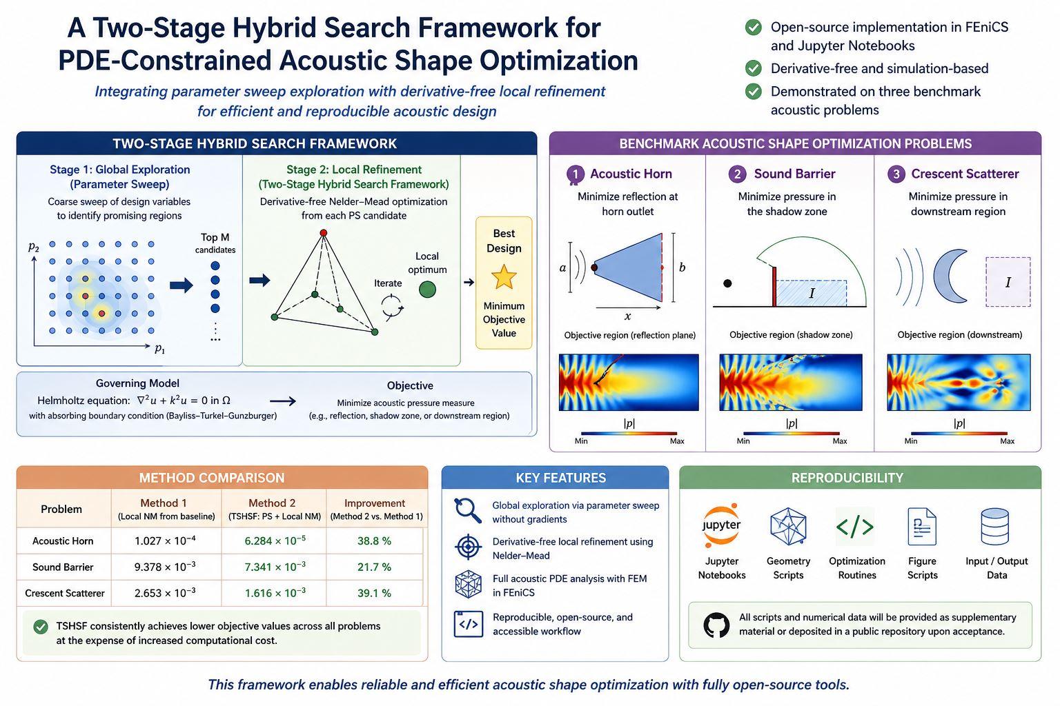
To overcome these limitations, this study introduces an open-source two-stage PS–NM workflow that combines a Parameter Sweep (PS) for feasibility assessment and coarse global exploration with penalty-augmented Nelder–Mead (NM) local refinement. The parameter sweep provides promising initial candidates without relying on gradients, while the NM stage locally refines the best candidates. By combining broad exploration with local refinement, the proposed workflow improves practical robustness relative to baseline-initialized local optimization in PDE-constrained acoustic design. The implementation is fully open-source, built on the FEniCS environment, and demonstrated on benchmark problems to showcase its accuracy and accessibility.

The proposed procedure should be interpreted as a reproducible open-source implementation of a standard global-search/local-refinement strategy rather than as a new abstract optimization algorithm. Combinations of grid search, multistart exploration, or other global screening procedures with local optimization are well established in numerical optimization. The contribution of the present work is the integration of this strategy with geometry generation, feasibility screening, finite element Helmholtz analysis, absorbing boundary treatment, and derivative-free local refinement for multiple acoustic shape-optimization benchmarks within an accessible FEniCS/Jupyter workflow.

Because the proposed framework is derivative-free and simulation-based, the reported optima should be interpreted as the best designs found within the chosen parameterization, parameter-sweep resolution, mesh resolution, and local-search settings. The method improves robustness relative to baseline-initialized local optimization, but it does not constitute a proof of global optimality. The novelty of the present work is not the introduction of a new abstract optimization algorithm, but the development of a fully open-source, end-to-end computational workflow that integrates geometry generation, feasibility screening, finite element Helmholtz analysis, and derivative-free shape optimization for multiple acoustic benchmark problems.

2. Problem Formulation and Optimization Framework

The goal of acoustic shape optimization is to determine the geometric configuration of a domain such that the acoustic field satisfies the design objective while obeying the Helmholtz equation and relevant physical constraints [17]. The general mathematical formulation of this problem can be expressed as:

$$\begin{array}{ccc}\hfill & \underset{\mathit{p}\in \mathcal{P}}{min}J(\mathit{p},u),\hfill & \hfill \mathrm{subject}\mathrm{to}\\ \hfill & {\nabla }^{2}u(\mathit{x};\mathit{p})+k^{2}u(\mathit{x};\mathit{p})=0,\hfill & \hfill \mathrm{in}\mathsf{\Omega },\\ \hfill & g(\mathit{p},u)=0,h(\mathit{p},u)\le 0.\hfill & \hfill \end{array}$$

(1)

In this formulation, $\mathit{p}\in \mathcal{P}$ denotes the vector of design variables, and $\mathit{x}$ denotes the spatial coordinates within the geometry. The state variable $u(\mathit{x};\mathit{p})$ satisfies the Helmholtz equation in the spatial domain $\mathsf{\Omega }$, where k is the angular wavenumber. The objective function $J(\mathit{p},u)$ can be constructed to represent acoustic pressure in a specified targeted region.

The equality constraint $g(\mathit{p},u)=0$ is used to enforce physical and geometric requirements such as boundary conditions or symmetry. The inequality constraint $h(\mathit{p},u)\le 0$ imposes limitations on the design, such as bounds on parameter values, shape area restrictions, or performance thresholds (e.g., a maximum allowable sound pressure level). These constraints ensure that the optimization remains feasible and avoids nonphysical or nonfunctional configurations.

The shape optimization problems addressed in this study fall within the category of constrained optimization, where the optimal shape is sought within a restricted subset of the design space. In this context, a feasible region is defined as the subset of the design space where all constraints are satisfied. A solution within this region is considered valid, while any shape that violates the optimization constraints is deemed infeasible. The challenge in constrained shape optimization is not only to find the shape corresponding to the optimum objective-function value but also to ensure that the optimization process operates within the feasible region [18]. One way to enforce this condition is to introduce a penalty function which applies a corrective penalty value when the search algorithm moves out of the feasible region. Hence, constraint violations are systematically accounted for during the optimization process.

Traditional local optimization methods, such as gradient-based techniques or direct search algorithms, often fail in the presence of multiple local minima. This issue is especially challenging in acoustic shape optimization, where wave-based objectives exhibit complex and highly non-convex landscapes. A global or hybrid strategy is therefore required to achieve reliable exploration of complex design spaces.

To address this, we adopt a two-stage PS–NM workflow. In the first stage, a Parameter Sweep (PS) is used to perform a coarse but systematic exploration of the design space, identifying promising candidates without relying on gradients. In the second stage, a penalty-augmented NM procedure refines these candidates locally. Importantly, the local-refinement stage is initialized with the PS results, starting from the best candidate and proceeding in descending order of performance when additional candidates are considered. This strategy focuses the local optimizer first on promising regions of the design space and reduces sensitivity to arbitrary initialization.

The following subsections describe the details of the PS method and the PS–NM local-refinement procedure.

2.1. Feasibility Analysis Using Parameter Sweep Method

The Parameter Sweep (PS) method, also known as brute-force search, optimizes a function by systematically evaluating a discrete set of possible parameter values. Each configuration is assessed, and the one yielding the most favorable outcome is selected [19]. While highly effective for small-scale problems, PS becomes computationally demanding in high-dimensional design spaces due to the exponential growth of combinations. Nevertheless, it remains a valuable tool when multiple parameters influence performance and their interactions are not well understood.

In the first stage of our framework, PS is used to explore the feasible region exhaustively and identify candidate designs that minimize the objective function while satisfying all constraints. Each candidate ${\mathit{p}}_i\in \mathcal{P}$ is first evaluated against explicitly defined geometric constraint functions $g\left({\mathit{p}}_i\right)=0$ and $h\left({\mathit{p}}_i\right)\le 0$, determining feasibility (${\mathit{p}}_i\in \mathcal{F}\subset \mathcal{P}$). Only feasible candidates are then meshed, solved with the Helmholtz equation, and evaluated with respect to the objective function $J({\mathit{p}}_i,u)$.

The proposed pre-screening strategy applies to constraints that depend solely on the design parameters. For problems involving performance-based or implicit constraints—such as limits on sound pressure levels that require evaluation of the state variable u—the Helmholtz equation must first be solved before feasibility can be assessed. In such cases, constraint verification is performed after state evaluation rather than during the preliminary screening stage.

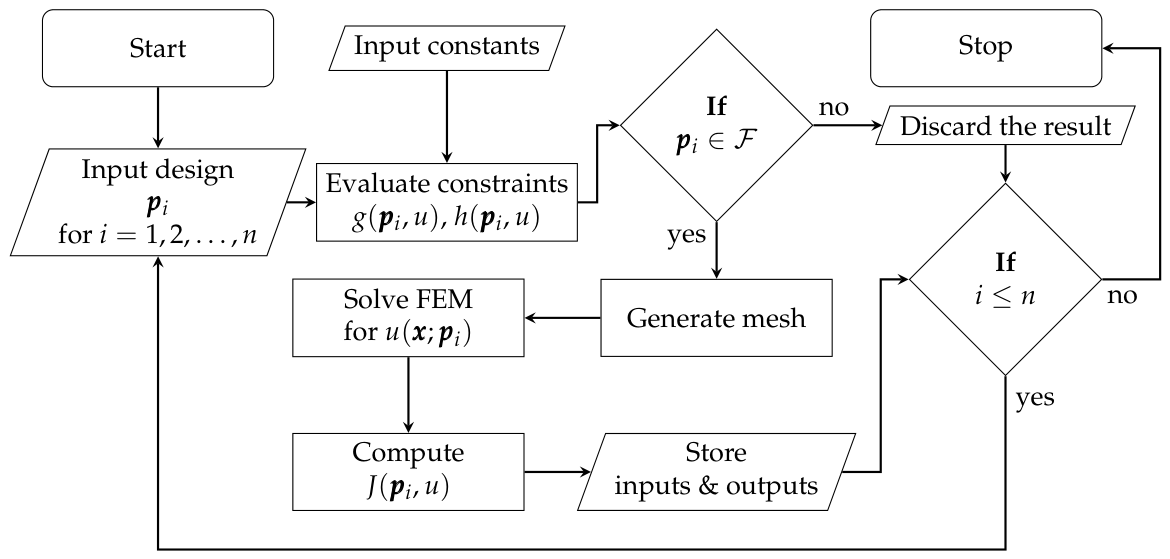
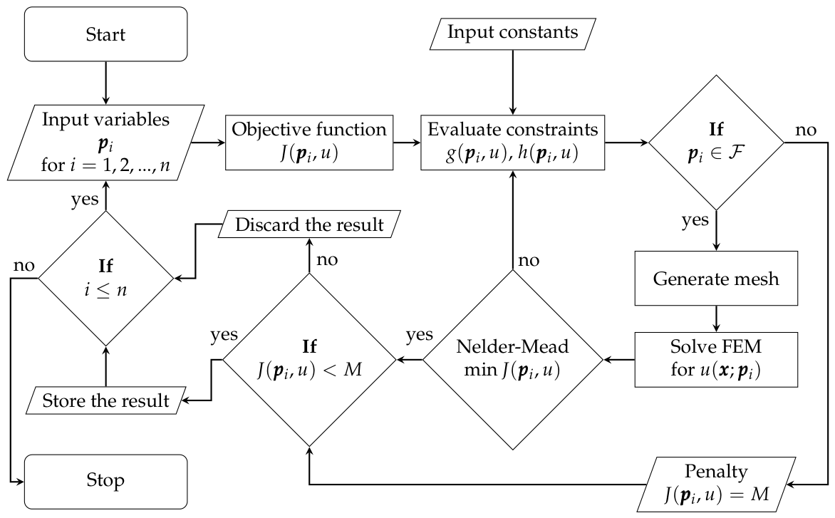
The workflow of the PS algorithm is illustrated in Figure 1. The diagram highlights the sequence of constraint evaluation, finite element solution, and objective calculation, iterated across the discrete design space. In this study, the PS method not only ensures that initial conditions for the optimization lie within the feasible region, but also ranks them by objective value. These ordered candidates are then passed to the NM local-refinement stage, beginning with the best-performing solution, thereby guiding the local refinement process efficiently.

2.2. Two-Stage PS–NM Workflow for Local Refinement

The scipy.optimize library provides various numerical optimization algorithms for finding the minimum of an objective function, including the Nelder–Mead (NM) method, which is well-suited for derivative-free optimization [20]. The NM algorithm is a direct search method that does not require gradient information, making it applicable to problems where derivatives are unavailable or expensive to compute.

The NM method is a simplex-based iterative technique designed to locate the minimum of an objective function. It operates by initializing a simplex in an n-dimensional parameter space and performing a series of transformations—including reflection, expansion, contraction, and shrinkage—to iteratively move toward the optimum [18,21]. Since its introduction, the method has been widely applied in diverse fields such as engineering, finance, and scientific computing. In acoustics, NM has been used to optimize material properties and geometric parameters of coatings [22], and to improve the efficiency of noise barriers [23].

Although effective for many applications, the classical NM algorithm is inherently a local optimizer. It is designed for local refinement and may converge to a local minimum or stagnate near a suboptimal configuration, especially in non-convex search spaces. Its performance is also sensitive to the initial simplex: poor initialization may prevent the algorithm from exploring the design space adequately, leading to premature convergence [16]. It is important to emphasize that the NM algorithm used in this work is a local derivative-free search procedure. Therefore, the final point obtained by NM should be interpreted as a locally refined solution associated with the selected initial simplex and the prescribed stopping tolerances, rather than as a globally optimal design. In non-convex Helmholtz optimization problems, different initial simplices may converge to different local minima or may stagnate near suboptimal configurations. The role of the preceding PS stage is therefore not to remove the local nature of NM, but to reduce its sensitivity to arbitrary initialization by supplying feasible and comparatively promising starting points. Consequently, the proposed PS–NM workflow improves practical robustness with respect to initialization, while no claim of mathematical global convergence is made.

To address these limitations in constrained acoustic problems, we use a two-stage PS–NM workflow. Here, “two-stage” refers to the combination of global exploration (PS) and local refinement (Nelder–Mead) within a unified implementation. The modification incorporates an exterior penalty treatment to handle constraint violations. In the present implementation, the penalty value is used as a hard rejection value rather than as a continuous penalty landscape. During the PS stage, candidates that violate purely geometric feasibility constraints are discarded before meshing and FEM solution. During the NM stage, if a trial simplex point violates the same feasibility checks, the objective function returns the fixed value M without solving the Helmholtz problem. Thus, the penalty is used only to steer the local optimizer away from infeasible geometries. In all numerical examples, $M=10$ was chosen to be larger than the feasible objective values encountered in the corresponding optimization runs; therefore, infeasible candidates cannot be preferred over feasible candidates. Nevertheless, this fixed-penalty strategy should be understood as a practical constraint-handling device, not as an exact penalty formulation. More sophisticated adaptive or constraint-aware penalty strategies could be incorporated in future extensions [17,24].

Crucially, the NM refinement is not initialized arbitrarily: it receives its starting points from the ranked PS candidates, beginning with the best-performing design and proceeding in descending order when additional candidates are refined. This strategy reduces sensitivity to initialization and improves the likelihood of finding a good local optimum within the selected computational budget. The search continues iteratively until user-defined convergence criteria are satisfied.

The workflow of the two-stage PS–NM procedure is illustrated in Figure 2. The proposed integration strategy allows the method to navigate constrained design spaces with improved practical robustness. When combined with the global feasibility analysis of the PS stage, the hybrid PS–NM workflow balances global exploration with efficient local refinement.

2.3. Interpretation of the Inverse Design Problem

The optimization problems considered in this study can be interpreted as inverse design problems: instead of predicting the acoustic field for a prescribed geometry only, the geometry is adjusted so that the computed acoustic field satisfies a desired performance criterion. For a fixed admissible geometry and fixed boundary conditions, the forward Helmholtz problem is deterministic after discretization. However, the inverse design problem is not necessarily unique. Different parameter vectors may generate geometrically distinct shapes with similar objective-function values, especially when the objective is defined as an integral over a target region rather than as a pointwise matching condition. In addition, the acoustic objective landscape is generally non-convex and frequency-dependent, so multiple local optima may coexist.

For this reason, the optimized parameters reported in this work should be understood as the best design variables found within the selected parameterization, parameter bounds, mesh resolution, parameter-sweep resolution, and local-search tolerances. Stability is assessed here in a numerical and practical sense: mesh and polynomial-order convergence studies are used to reduce discretization sensitivity, while the PS initialization reduces sensitivity to arbitrary local-search starting points. Nevertheless, the method does not establish uniqueness of the inverse design solution, nor does it provide a theorem guaranteeing continuous dependence of the optimizer on perturbations of the objective, frequency, or discretization. These limitations are consistent with the derivative-free and simulation-based nature of the proposed framework.

2.4. Absorbing Boundary Condition

In the finite element solution of exterior Helmholtz problems, an absorbing boundary condition is required to simulate the radiation of acoustic waves into an unbounded domain. Without such a condition, artificial reflections from the truncated boundary would contaminate the numerical solution. To accurately approximate wave behavior at infinity while keeping the computational domain finite, an absorbing boundary condition is imposed on the outer artificial boundary ${\mathrm{\Gamma }}_{\mathrm{R}}$. This is achieved by approximating the exact radiation condition through a Dirichlet-to-Neumann (DtN) map. In this study, we employ the Bayliss–Gunzburger–Turkel (BGT) absorbing boundary condition, a widely used high-order approximation to the DtN operator for wave scattering problems. Alternatively Padé type and Farfield Expansion absorbing boundary conditions developed for both single- and multiple-scattering analyses can be used with the framework developed in the study directly [25,26,27,28].

On the outer boundary of the computational domain ${\mathrm{\Gamma }}_{\mathrm{R}}$ the scattered field $u_{\mathrm{s}}$ satisfies:

$${\displaystyle \frac{\partial u_{\mathrm{s}}}{\partial r}}=B{u}_{\mathrm{s}}\mathrm{on}{\mathrm{\Gamma }}_{\mathrm{R}},$$

(2)

where the operator B approximates the DtN map using the BGT condition. The general form of the m-th order BGT condition is given by:

$${\mathrm{BGT}}_m={\displaystyle \prod _{j=1}^m}\left({\displaystyle \frac{\partial }{\partial r}}-ik+{\displaystyle \frac{4j-3}{2r}}\right),m\ge 1,$$

(3)

where r is the radial coordinate and k is the angular wavenumber.

In the finite element implementation, this condition enters the weak form through the corresponding boundary integral over ${\mathrm{\Gamma }}_R$, replacing the exact exterior radiation condition by the selected BGT approximation. The horn and barrier examples use the first-order BGT condition, whereas the crescent example uses the second-order BGT condition.

3. Validation Using Benchmark Problems

To assess the performance of the proposed shape optimization framework, three benchmark problems are introduced in the following sections, illustrating the application of the hybrid optimization approach to wave scattering and noise control. In all cases, the governing physics is based on the Helmholtz equation, with optimization objectives focusing on minimizing scattered wave energy, reducing reflections, or attenuating acoustic pressure in target regions. These test cases evaluate the framework’s effectiveness in constrained shape optimization for acoustics.

To make the finite-dimensional inverse design setting explicit, the number of optimized geometric parameters is stated for each benchmark problem. In the acoustic horn problem, the coordinates of either one or two B-spline control points are optimized, corresponding to two design variables, $(x_1,y_1)$, or four design variables, $(x_1,y_1,x_2,y_2)$, respectively. In the sound barrier problem, the optimized design vector consists of the horizontal coordinates of the B-spline control points defining the variable front face of the barrier; hence, the number of optimized parameters is $N=5,10,15$, or 20, depending on the case considered. In the crescent-shaped scatterer problem, two geometric parameters are optimized: the radius of the secondary cropping cylinder, $r_2$, and its horizontal offset, $d_x$. In the following sections, these parameters are referred to as optimized geometric design variables rather than recovered material or field parameters, since the present work addresses shape optimization rather than parameter identification.

3.1. Acoustic Horn Problem

Acoustic horns are widely used to enhance sound transmission efficiency by providing impedance matching between a source and the surrounding medium. They are commonly employed in loudspeakers, musical instruments, and industrial applications where controlled wave propagation is essential. The primary objective of optimizing an acoustic horn’s geometry is to maximize wave transmission into the far field while minimizing reflections and energy losses, as in Bångtsson et al. [5], Wadbro et al. [29], Farhadina [30], Barbieri et al. [31], Shaaban et al. [32], Ummudivarapu et al. [33], Khajah et al. [34], and Videla et al. [35]. These references employ various shape optimization techniques such as isogeometric analysis [36], boundary element methods [37], genetic algorithms [38], and quasi-Newton methods [39].

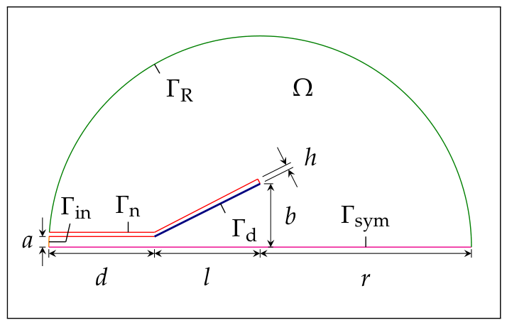
This section considers the shape optimization of an acoustic horn, where the geometry of the horn’s boundary, denoted as ${\mathrm{\Gamma }}_{\mathrm{d}}$, is adjusted to improve energy transmission. The geometric configuration of the acoustic horn model is shown in Figure 3. The computational domain $\mathsf{\Omega }$ represents a half-cylinder with rigid boundaries ${\mathrm{\Gamma }}_{\mathrm{n}}$ and a planar symmetry at ${\mathrm{\Gamma }}_{\mathrm{sym}}$. An incident acoustic wave impinges on the horn, and the scattered field is analyzed to assess the effectiveness of the design in achieving impedance matching with the surrounding medium.

The problem is formulated as an acoustic scattering problem, where a time-harmonic plane wave impinges on the boundary ${\mathrm{\Gamma }}_{\mathrm{in}}$ within the computational domain $\mathsf{\Omega }$. The governing equation is the Helmholtz equation:

$${\mathsf{\nabla }}^{2}u+k^{2}u=0\mathrm{in}\mathsf{\Omega },$$

(4)

where u represents the complex acoustic pressure field and k is the angular wave number.

At the inlet boundary ${\mathrm{\Gamma }}_{\mathrm{in}}$, a Robin condition models the overlapping plane wave:

$${\displaystyle \frac{\partial u}{\partial \mathit{n}}}+iku=2ik{A}_m\mathrm{on}{\mathrm{\Gamma }}_{\mathrm{in}},$$

(5)

where $A_m$ represents the amplitude of the incoming wave. The rigid walls of the horn, denoted by ${\mathrm{\Gamma }}_{\mathrm{n}}$, satisfy a Neumann boundary condition, which enforces no normal wave flux:

$${\displaystyle \frac{\partial u}{\partial \mathit{n}}}=0\mathrm{on}{\mathrm{\Gamma }}_{\mathrm{n}}.$$

(6)

Similarly, the symmetry boundary ${\mathrm{\Gamma }}_{\mathrm{sym}}$ is also subject to a homogeneous Neumann condition:

$${\displaystyle \frac{\partial u}{\partial \mathit{n}}}=0\mathrm{on}{\mathrm{\Gamma }}_{\mathrm{sym}}.$$

(7)

At the outlet boundary ${\mathrm{\Gamma }}_{\mathrm{R}}$, an absorbing boundary condition is applied to minimize reflections from the artificial truncation of the domain. This is implemented using the BGT-1 formulation described in Section 2.4.

The goal of the optimization is to minimize the wave reflection coefficient R, defined as

$$R={\displaystyle \frac{B_m}{A_m}}\mathrm{on}{\mathrm{\Gamma }}_{\mathrm{in}},$$

(8)

where $A_m$ is the amplitude of the incident wave, and $B_m$ denotes the reflected wave amplitude. The latter is estimated by comparing the average acoustic pressure on the inlet boundary to the known incident amplitude:

$$B_m=\left|u_{\mathrm{in}}-A_m\right|,$$

(9)

where $u_{\mathrm{in}}$ is the mean acoustic pressure over ${\mathrm{\Gamma }}_{\mathrm{in}}$, given by

$$u_{\mathrm{in}}={\displaystyle \frac{1}{a}}{\int }_{{\mathrm{\Gamma }}_{\mathrm{in}}}u\mathrm{d}\mathrm{\Gamma },$$

(10)

with a denoting the width of the inlet boundary. Accordingly, the optimization objective function is formulated as $J\left(u\right)=R$. The reflection coefficient R is non-negative by construction, and in well-posed scattering problems with minimal numerical artifacts, it typically satisfies $R\le 1$. However, in practice, values slightly exceeding one may arise due to numerical approximations or local interference effects.

The initial horn geometry is characterized by a constant thickness $h=2.5$ cm. The inlet width and outlet width are defined as $a=5$ cm and $b=30$ cm, respectively. The horn consists of a straight section of length $d=50$ cm, followed by a flaring section of length $l=50$ cm. The incident wave amplitude is set to $A_m=1$, and the radius of curvature at the outlet boundary ${\mathrm{\Gamma }}_{\mathrm{R}}$ is taken as $r=1$ m.

The numerical analysis is performed for four frequencies: 280 Hz, 400 Hz, 550 Hz, and 780 Hz, considering the coordinates of 1 and 2 control points of the B-spline representing the boundary ${\mathrm{\Gamma }}_{\mathrm{d}}$ as design variables for shape optimization.

The shape of the horn boundary ${\mathrm{\Gamma }}_{\mathrm{d}}$ is parameterized using a B-spline representation, ensuring a smooth geometric transformation during the optimization process. A set of control points defines the boundary shape to increase flexibility in modifying the horn profile while maintaining geometric constraints. The optimization considers configurations with both 1 and 2 control points, which influence the degree of geometric variation. The results of the scattering analysis inform the optimization of the boundary ${\mathrm{\Gamma }}_{\mathrm{d}}$, enabling the reduction of backscattering and the enhancement of forward energy transmission.

The design constraints were enforced using a feasibility check that ensures the optimized shape remains within predefined geometric bounds. The feasible region is defined based on the initial horn geometry. Any shape modifications that violate these constraints are penalized in the optimization process. The constraints are verified using B-spline approximation and a polygonal feasibility check, preventing self-intersecting or impractical horn shapes. The entire numerical workflow, including mesh generation, shape parameterization, and constraint verification, is implemented in Python 3.6.9 using Gmsh Python API 4.11.1 for meshing, SciPy 0.19.1 for B-spline interpolation, and FEniCS 2019.1.0 for FEM-based acoustic analysis.

3.2. Sound Barrier Problem

The design of noise barriers plays a critical role in minimizing sound transmission beyond the protected region. Key factors influencing barrier effectiveness include its geometry, material properties, and placement. Previous studies have demonstrated that modifying the shape and composition of noise barriers can significantly improve their sound attenuation performance. Ishizuka and Fujiwara [40] analyzed the effect of barrier height and angular placement on diffraction and refraction of sound waves using the Boundary Element Method (BEM). Toledo et al. [41] introduced hybrid modeling approaches, combining finite and boundary elements, and investigated the use of composite materials to enhance sound insulation. Their findings indicate that integrating absorptive and reflective materials at the upper edges of barriers effectively reduces high-frequency sound diffraction.

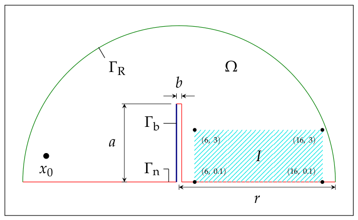
In this section, we consider a rigid vertical noise barrier with an infinite out-of-plane length and a variable front-face geometry. A schematic of the geometry of the problem is shown in Figure 4. The objective is to minimize the acoustic pressure in the shaded area behind the barrier by optimizing its shape. The barrier extends from (5, 0) to (5, 3), with a fixed height of $a=3$ meters and an initial thickness of $b=0.2$ meters. A monopole line source is placed at ${\mathit{x}}_0=(0,1)$ in front of the barrier, emitting a time-harmonic acoustic wave. The shape optimization process modifies the x-coordinates of several B-spline control points while keeping their y-coordinates fixed. These control points are auxiliary parameters used to generate the smooth barrier profile and should not be interpreted as physical points on the barrier surface. The physical feasibility constraints are imposed on the evaluated B-spline curve representing the actual barrier front face, not directly on the individual control-point coordinates. The initial control-point x-coordinates are set at 5.0 m, and the resulting spline-generated barrier profile is constrained to remain within the prescribed geometric bounds.

The total acoustic wave field, u, is composed of the incident wave generated by the point source, $u_G$, and the scattered wave, $u_{\mathrm{s}}$:

$$u=u_G+u_{\mathrm{s}}.$$

(11)

The incident wave $u_G$ satisfies the Helmholtz equation with a monopole source term. The sign of the source term is written consistently with the Green’s function convention adopted in Equation (14); using the alternative time-harmonic convention would reverse the signs of both the source term and the fundamental solution without changing the magnitude-based objective used here:

$${\mathsf{\nabla }}^2{u}_G+k^2{u}_G=\delta (\mathit{x}-{\mathit{x}}_0)\mathrm{in}\mathsf{\Omega },$$

(12)

where $\delta (\mathit{x}-{\mathit{x}}_0)$ is the Dirac delta function modeling a point source at location ${\mathit{x}}_0$. The boundary condition for $u_G$ on the rigid boundary ${\mathrm{\Gamma }}_{\mathrm{n}}$ is:

$${\displaystyle \frac{\partial u_G}{\partial n}}=0\mathrm{on}{\mathrm{\Gamma }}_{\mathrm{n}}.$$

(13)

Instead of solving for $u_G$ directly using a variational formulation, we utilize the Green’s function for a half-plane, given by:

$$G(\mathit{x},{\mathit{x}}_0)=-{\displaystyle \frac{i}{4}}{H}_0^{\left(1\right)}\left(k\right|\mathit{x}-{\mathit{x}}_0\left|\right)-{\displaystyle \frac{i}{4}}{H}_0^{\left(1\right)}\left(k\right|\mathit{x}-{\overline{\mathit{x}}}_0\left|\right),$$

(14)

where ${\overline{\mathit{x}}}_0=(x_0,-y_0)$ represents the image source reflected across the symmetry boundary. This satisfies the Sommerfeld radiation condition at infinity. The scattered field $u_{\mathrm{s}}$ satisfies the homogeneous Helmholtz equation:

$$\mathsf{\Delta }{u}_{\mathrm{s}}+k^2{u}_{\mathrm{s}}=0\mathrm{in}\mathsf{\Omega }.$$

(15)

Boundary conditions are imposed on ${\mathrm{\Gamma }}_{\mathrm{b}}$ (the barrier surface), ${\mathrm{\Gamma }}_{\mathrm{n}}$ (rigid ground), and ${\mathrm{\Gamma }}_R$ (absorbing boundary) as follows: On the barrier surface ${\mathrm{\Gamma }}_{\mathrm{b}}$, the scattered wave satisfies:

$${\displaystyle \frac{\partial u_{\mathrm{s}}}{\partial \mathit{n}}}=-{\displaystyle \frac{\partial u_G}{\partial \mathit{n}}}\mathrm{on}{\mathrm{\Gamma }}_{\mathrm{b}}.$$

(16)

On the rigid ground ${\mathrm{\Gamma }}_{\mathrm{n}}$, the Neumann boundary condition ensures no normal flux:

$${\displaystyle \frac{\partial u_{\mathrm{s}}}{\partial \mathit{n}}}=0\mathrm{on}{\mathrm{\Gamma }}_{\mathrm{n}}.$$

(17)

On the outer artificial boundary ${\mathrm{\Gamma }}_{\mathrm{R}}$ which truncates the solution domain at $r=6$ m, an absorbing boundary condition is applied using the first-order BGT formulation to simulate outgoing wave radiation. The full formulation of the BGT condition is provided in Section 2.4. The optimization procedure aims to minimize the acoustic pressure in the shadow zone behind the barrier. The shape of the barrier is modified by adjusting the x-coordinates of control points along ${\mathrm{\Gamma }}_{\mathrm{b}}$, while ensuring that the modified geometry adheres to predefined constraints. This approach is similar to previous shape optimization studies that employed isogeometric methods [32,35,42].

Preliminary mesh generation tests used lower discretization settings to verify the geometry construction and boundary labeling. The final results reported below use the discretization selected from the convergence study in Section 3.4, namely $p=3$ and $n_{\lambda }=30$.

The computational domain is meshed using $n_{\lambda }=30$ elements per wavelength. A function-space order of $p=3$ is used for the FEM formulation. The mesh generation process enforces a tolerance of $0.01$ to properly define the domain boundaries.

The barrier’s front face geometry is parameterized using a B-spline representation, allowing a smooth and continuous modification of the shape. The B-spline resolution is set to $b{s}_{\mathrm{res}}=1000$, with a B-spline degree of $b{s}_{\mathrm{degree}}=3$, ensuring sufficient flexibility in capturing shape variations. Here, $b{s}_{\mathrm{res}}$ denotes the number of discrete sample points used to evaluate the B-spline curve along the barrier’s front face. These sampled points, rather than the B-spline control points themselves, define the physical barrier profile used in geometric feasibility checks. Consequently, individual control points may lie outside the physical bounds, provided that the evaluated spline curve remains within the admissible geometric region and satisfies the prescribed area and non-intersection constraints.

A constraint verification function ensures that the barrier does not significantly increase the total structural area while the acoustic efficiency of the barrier is increased. The area below the original barrier reference line is monitored, and constraints are enforced to prevent unwanted geometry violations.

The optimization objective function J is computed as the integral of the total wave magnitude over a rectangular region I located in the acoustic shadow behind the barrier. The region is defined by the bounds $I=\left\{\right(x,y)\in \mathsf{\Omega }:x\in [6,16],y\in [0.1,3\left]\right\}$, and the functional is given by

$$J={\int }_I\left|u\right|\mathrm{d}\mathsf{\Omega }.$$

(18)

The numerical simulations and optimizations were implemented in Python, utilizing Gmsh for mesh generation, SciPy’s B-spline interpolation of the optimized boundary, and FEniCS for the FEM-based acoustic analysis.

To explore the design space and initialize the optimization with feasible candidates, a Parameter Sweep (PS) method is employed. For small numbers of design parameters ($N=5,10$), the feasible region is discretized and fully enumerated, evaluating the objective function for all combinations.

However, for larger parameter sets ($N=15,20$), full enumeration becomes computationally prohibitive due to the exponential growth in design combinations. In these cases, we first estimate the number of possible configurations as:

$$C={\displaystyle \prod _{j=1}^N}\left(⌊{\displaystyle \frac{p_j^{max}-p_j^{min}}{\Delta p_j}}⌋+1\right),$$

(19)

In this expression, the index j runs over the N design variables that make up the design vector $\mathit{p}=(p_1,p_2,\dots ,p_N)$. For each variable $p_j$, the term $⌊\frac{p_j^{max}-p_j^{min}}{\Delta p_j}⌋+1$ gives the number of discrete values it can take under the specified bounds and increment. The product therefore counts all possible combinations across variables, yielding C as the total number of candidate design vectors ${\mathit{p}}_i$, with $i=1,\dots ,C$. Here, j indexes parameter dimensions, while i indexes complete candidate vectors in the discretized design space.

When the computed number of combinations exceeds the practical budget, the exhaustive PS stage is replaced by a budget-limited uniform random sampling strategy. Random search is a standard stochastic global-search approach when exhaustive grid enumeration is impractical, especially in high-dimensional parameter spaces [43,44,45]. In the present implementation, the switch at $C>{10}^4$ was selected as a practical computational limit for the available hardware and wall-clock time, rather than as a theoretical convergence threshold. Therefore, the random sampling stage should be interpreted as a heuristic feasibility-screening procedure, not as a probabilistic guarantee of global coverage. This limitation is important in high-dimensional cases, where uniform random samples may still leave parts of the design space unexplored. The purpose of the random PS stage is to provide improved initial candidates for subsequent NM refinement, rather than to certify global optimality.

The PS resolution should be distinguished from the FEM discretization parameters discussed later in Section 3.4, “Numerical Discretization Parameters”. The FEM convergence study controls the numerical accuracy of each acoustic simulation, whereas the PS resolution controls how densely the design-variable space is explored before NM refinement. A finer PS grid may provide a better initial candidate for NM, but it also increases the number of FEM solves and the total runtime. Therefore, in this study the PS resolution was selected as a practical compromise between design-space exploration and computational cost.

3.3. Crescent Problem

Next, we consider optimizing the shape of a crescent obstacle to minimize the acoustic pressure in a downstream target region for specified wavenumbers. Inspired by the geometric principle of cavity-type acoustic resonators, the crescent geometry is examined here as a lossless scattering structure capable of redistributing the acoustic field and reducing downstream pressure amplitude. Unlike a classical Helmholtz resonator with explicit losses, the present model does not evaluate acoustic absorption or dissipation; its performance is interpreted in terms of scattering, interference, and field redistribution.

Helmholtz resonators are widely used in exhaust systems for engine noise attenuation [46], industrial ventilation systems to reduce airflow noise [47], and building acoustics for controlling unwanted sound reflections [48]. In recent years, the development of acoustic metamaterials has further expanded interest in Helmholtz resonators, with studies investigating their geometric modifications and spatial arrangements to optimize performance [49,50,51,52].

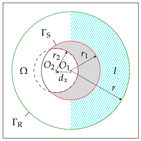
A novel crescent-shaped geometry is introduced as a tunable scattering obstacle inspired by cavity-type acoustic resonators. The geometry is constructed by defining a primary cylinder of radius $r_1$, centered at $O_1$, and a secondary cylinder of radius $r_2$, offset by a distance $d_x$ along the x-axis from $O_2$. The intersection of these two cylinders creates a crescent-shaped scattering object, as illustrated in Figure 5. By adjusting the radii and offset distance, the scattering characteristics and frequency-dependent response of the geometry can be modified.

While no prior research specifically investigates crescent-shaped scatterers for acoustic wave applications, studies on curved wave scattering obstacles provide valuable insights. Li et al. [53] analyzed ocean wave focusing by a submerged crescent-shaped plate using the Boundary Element Method (BEM), demonstrating how curved surfaces influence wave behavior. Similarly, Kowalczyk et al. [54] examined electromagnetic wave scattering from crescent-shaped cross-sections using a hybrid FEM-mode matching technique, validating the method’s accuracy against alternative numerical approaches.

Due to the lack of prior studies optimizing such a geometry, an initial brute-force parameter sweep was conducted across all design variables to explore the solution space. Subsequently, the two-stage PS–NM workflow was used to refine the best candidates obtained from the sweep.

A Bayliss–Gunzburger–Turkel (BGT-2) absorbing boundary condition was applied on ${\mathrm{\Gamma }}_{\mathrm{R}}$. Geometric constraints were imposed based on the relative positioning of the cropping and cropped cylinders to avoid unacceptable/non-physical shapes during optimization. If the cropping cylinder fully covers the primary cylinder, no scattering object remains. If the cropping cylinder remains entirely inside the primary cylinder, the scatterer reduces to a simple circular cylinder with no resonant cavity. If the cropping cylinder does not intersect the primary cylinder, the geometry reverts to a standard cylindrical scatterer.

The domain is defined by a primary cylinder of radius $r_1=1$ at the origin $(x,y)=(0,0)$, and a secondary cropping cylinder with variable radius $r_2$ and an x-axis offset distance $d_x$ from the primary cylinder. The absorbing boundary radius is dynamically computed as:

$$r=r_1+{\displaystyle \frac{2\pi }{k}},$$

(20)

where k represents the angular wavenumber.

A geometric feasibility check ensures that the cropping cylinder does not completely overlap or remain fully inside the primary cylinder. The optimization objective function J is computed as the integral of the total wave magnitude over a right-half target region I of the domain:

$$J={\int }_I\left|u\right|\mathrm{d}\mathsf{\Omega }.$$

(21)

The computational grid dynamically adapts to different values of $(r_2,d_x)$. All analyses were performed for wavenumbers $k=5$, $k=10$, and $k=15$, corresponding to different incident wavelengths.

These numerical settings ensure a balance between accuracy and computational efficiency while enabling systematic exploration of crescent-shaped geometries for acoustic wave control.

3.4. Numerical Discretization Parameters

The finite element method (FEM) discretization employed in this study uses triangular elements with Lagrange basis functions of degree p, corresponding to finite element spaces of type $P_p{\wedge }^0\left({\Delta }_2\right)$ in finite element exterior calculus notation [55]. Here, $P_p$ indicates Lagrange elements of polynomial degree p, ${\wedge }^0$ denotes discretization in the Sobolev space $H^1$, and ${\Delta }_2$ refers to triangular elements in a two-dimensional domain.

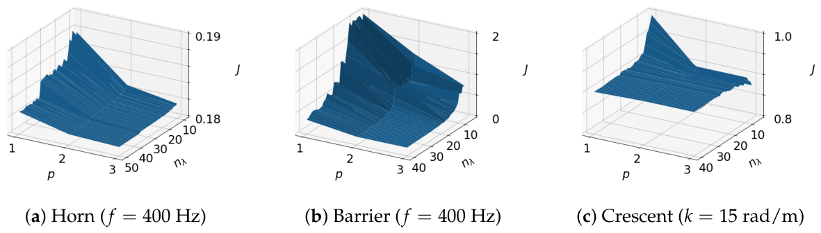
To ensure that the numerical results are not sensitive to mesh granularity or basis order, convergence analyses were systematically conducted for all horn frequencies ($f=280$, 400, 550, and 780 Hz), the sound barrier problem at $f=400$ Hz, and the crescent-shaped scatterer problem at $k=5$, 10, and 15 rad/m. In each case, the objective function J of the corresponding benchmark problem was evaluated as a function of the discretization density $n_{\lambda }$ (elements per wavelength) and the finite element polynomial order p. Representative results of these convergence studies are illustrated in Figure 6, showing the trends observed in three of the most sensitive configurations.

The convergence results revealed that third-order basis functions ($p=3$) and a discretization density of $n_{\lambda }=30$ elements per wavelength were sufficient to achieve mesh-independent solutions in the most sensitive configurations (notably at $f=400$ Hz and $k=15$ rad/m). Based on these findings, all subsequent simulations adopt $p=3$ and $n_{\lambda }=30$ to balance numerical accuracy with computational efficiency.

Analytical expressions required for the incident wave field and other auxiliary fields are interpolated into the FEM space using an interpolation polynomial of degree q, referred to as the expression-degree. This ensures consistency between analytical inputs and the FEM approximation space, and minimizes projection errors during computation.

4. Results

The proposed optimization framework was applied to three benchmark problems: the acoustic horn, the sound barrier, and the crescent-shaped scatterer. In each case, two optimization strategies were evaluated:

• Method 1: baseline-initialized penalty-augmented Nelder–Mead optimization.
• Method 2: two-stage PS–NM workflow, consisting of Parameter Sweep (PS) initialization followed by penalty-augmented Nelder–Mead refinement.

For each benchmark, the results are reported in tabular form with the following quantities:

• DOF: number of degrees of freedom in the FEM discretization,
• $n_{\mathrm{PS}}$: number of candidate evaluations during the parameter sweep (Method 2 only),
• $n_{\mathrm{NM}}$: number of NM iterations within Method 2, counted only for the top-ranked PS candidate (best-first initialization),
• t: total wall–clock runtime in seconds,
• J: objective function value (reflection coefficient for the horn, integrated pressure in the shadow region for the barrier and crescent),
• control point coordinates: design variables defining the optimized geometry.

In Method 2, the NM refinement was initialized exclusively with the top-ranked PS candidate to ensure consistency and efficiency. Although subsequent candidates could also be refined, potentially yielding further improvements, this study adopts a best-first strategy to reflect a practical balance between accuracy and computational cost.

This common reporting structure allows a direct comparison of Method 1 and Method 2 in terms of objective value, iteration counts, and computational time. Across all benchmarks, Method 2 consistently achieved lower objective values, at the cost of higher runtime due to the PS stage.

Comparisons with published benchmark results support the accuracy and consistency of the implementation. This dual comparison highlights both the accuracy of the numerical framework and the effectiveness of the proposed two-stage optimization strategy.

4.1. Acoustic Horn Optimization Results

The proposed shape optimization framework was applied to the acoustic horn to enhance transmission efficiency and minimize backscattering. Optimizations were performed at frequencies $f\in \{280,400,550,780\}\mathrm{Hz}$. The horn boundary ${\mathrm{\Gamma }}_{\mathrm{d}}$ is parameterized by a cubic B–spline; the optimization adjusts control point coordinates to produce a smooth flare profile that improves impedance matching and reduces reflections relative to the baseline (pre-optimization) geometry. Two design scenarios were considered: (i) one control point (two design variables) and (ii) two control points (four design variables).

For each frequency and scenario, we compare Method 1 (baseline-initialized penalty-augmented Nelder–Mead) against Method 2 (PS-initialized penalty-augmented Nelder–Mead), reporting the final objective $J\left(u\right)=R$, iteration counts, and wall-clock time.

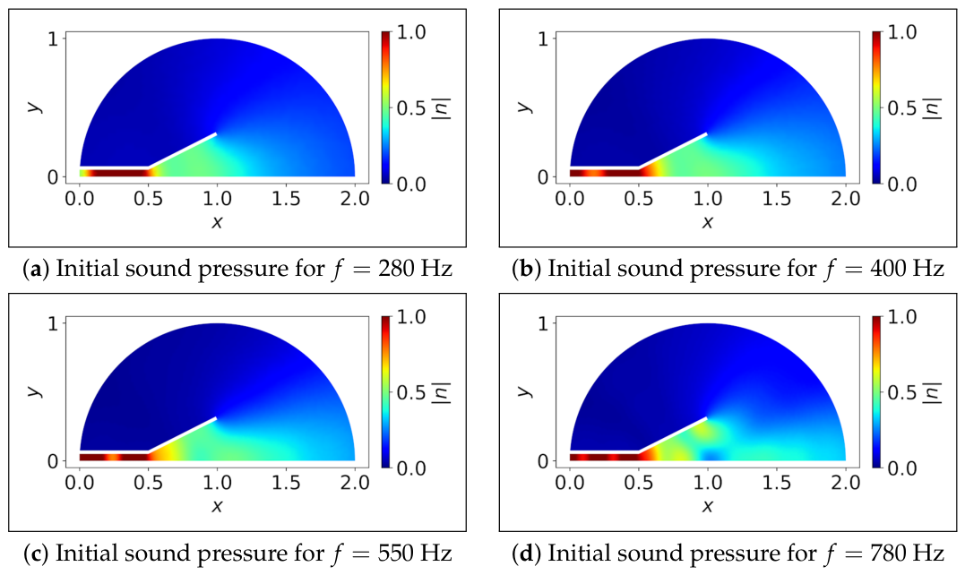
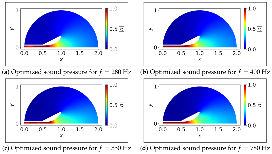
Figure 7 presents the sound pressure distributions at selected frequencies for the initial horn shape and Figure 8 presents the sound pressure distributions at each frequency after optimization using one control point with two design variables.

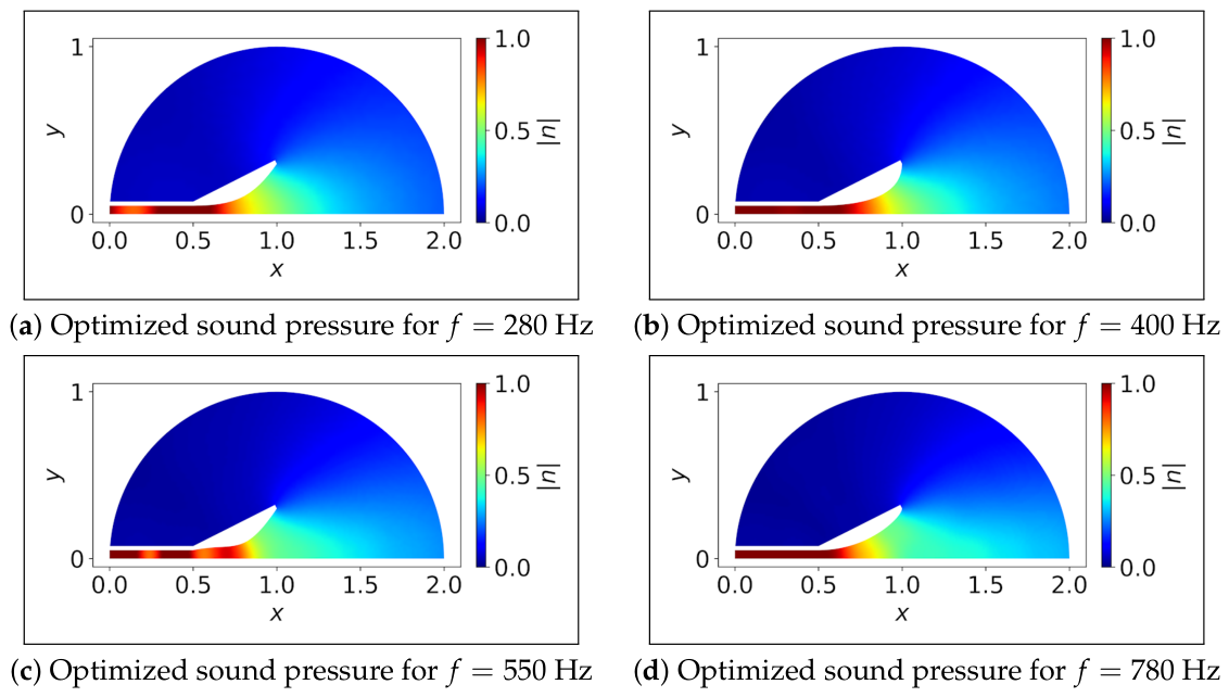
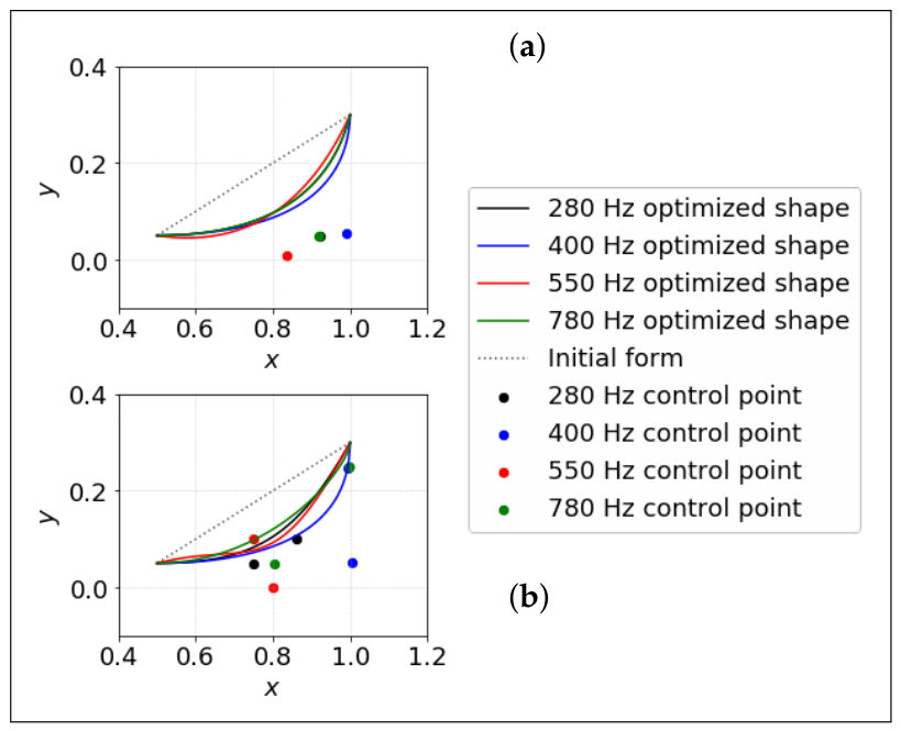
Figure 9 presents the sound pressure distributions at selected frequencies for the optimized horn shapes obtained using two control points with four variables. The final horn profiles in both cases demonstrate a gradual flaring at the outlet, which is consistent with findings in prior studies. Figure 8 and Figure 9 show a reduction in dark bands within the waveguide, indicating significantly lower wave reflections in the optimized horn designs.

The B-Spline curve designs obtained for all frequencies are shown in Figure 10 for both one-control-point and two-control-point solutions.

Table 1. Optimization results for horn with one control point.

f (Hz)	Method	DOF	${\mathit{n}}_{\mathbf{PS}}$	${\mathit{n}}_{\mathbf{NM}}$	t (s)	J	x	y
280	1	11,200	–	27	14.9	0.01883	0.990	0.060
	2	11,686	810	15	247.7	0.00060	0.921	0.050
400	1	21,952	–	10	16.0	0.18108	0.750	0.175
	2	21,226	102	20	68.9	0.00029	0.99	0.054
550	1	43,579	–	10	30.1	0.01082	0.750	0.175
	2	42,772	24	12	52.0	0.00006	0.835	0.01
780	1	81,136	–	10	57.8	0.093556	0.750	0.175
	2	79,474	206	10	413.4	0.01247	0.920	0.050

reports the optimization results for the horn with one control point (two design variables). Across all tested frequencies, Method 2 consistently achieved significantly lower reflection coefficients J than Method 1 (baseline-initialized NM). At 280 Hz, for example, J decreased from $1.9\times {10}^{-2}$ to $6.0\times {10}^{-4}$, representing more than an order of magnitude improvement. Similar reductions are observed at 400, 550, and 780 Hz.

This improvement comes at the cost of additional runtime: Method 2 required substantially longer wall–clock times due to the PS stage, particularly at the highest frequency where the runtime increased from 58 s to 413 s. Nevertheless, the number of NM iterations $n_{\mathrm{NM}}$ did not increase markedly, since the PS stage provided high-quality initial candidates.

The optimized control-point coordinates produce modest but systematic modifications of the spline-generated horn boundary. The resulting profiles remain smooth and geometrically feasible while improving the impedance transition between the inlet and the radiating region. These modifications reduce backscattering relative to the baseline-initialized local optimization.

Table 2. Optimization results for horn with two control points.

f (Hz)	Method	DOF	${\mathit{n}}_{\mathbf{PS}}$	${\mathit{n}}_{\mathbf{NM}}$	t (s)	J	${\mathit{x}}_1$	${\mathit{y}}_1$	${\mathit{x}}_2$	${\mathit{y}}_2$
280	1	11,539	–	54	32.0	$2.38\times {10}^{-4}$	0.949	0.102	0.977	0.056
	2	11,857	661	32	225.4	$3.34\times {10}^{-5}$	0.748	0.05	0.861	0.101
400	1	21,223	–	10	8.6	$1.81\times {10}^{-1}$	0.667	0.133	0.833	0.217
	2	21,235	123	35	103.1	$8.49\times {10}^{-5}$	1.005	0.051	0.995	0.248
550	1	42,895	–	10	16.6	$1.10\times {10}^{-2}$	0.667	0.133	0.833	0.217
	2	42,889	43	18	95.7	$2.64\times {10}^{-5}$	0.748	0.101	0.800	0.000
780	1	78,139	–	10	32.8	$9.27\times {10}^{-2}$	0.667	0.133	0.833	0.217
	2	79,783	55	19	218.5	$4.35\times {10}^{-6}$	0.802	0.050	0.998	0.249

summarizes the results for the two-control-point case (four design variables). Compared to the single–control–point case, the additional design freedom allowed the optimizer to achieve markedly lower reflection coefficients J, especially when using Method 2. For example, at 400 Hz, the hybrid method reduced J from $1.8\times {10}^{-1}$ to $8.5\times {10}^{-5}$, a reduction of more than three orders of magnitude. Similar trends are observed at all frequencies, with Method 2 consistently outperforming Method 1 in terms of objective value.

The cost of these improvements is evident in the runtimes: hybrid optimization required substantially more computational effort, particularly at higher frequencies where both the FEM system size and the number of PS samples increase. Nevertheless, the number of NM iterations $n_{\mathrm{NM}}$ remained moderate, again reflecting the benefit of high–quality initialization from the PS stage.

The optimized control point coordinates show that the horn boundary adapts flexibly to frequency: the first point primarily adjusts the throat region while the second modifies the flare toward the outlet. These coordinated adjustments enable smoother impedance transitions and stronger suppression of reflections. Overall, the two-control-point parameterization highlights the capability of the PS–NM workflow to exploit additional geometric freedom and deliver substantial acoustic performance gains, albeit at increased computational cost.

The large differences between Method 1 and Method 2 in Table 1 and Table 2 are attributed to the non-convex, interference-dominated objective landscape of the horn problem. Baseline-initialized NM explores only the local basin associated with the initial horn profile and the prescribed initial simplex. In several cases, the local search remains close to the initial control-point configuration or converges to a nearby suboptimal flare. The PS stage evaluates geometrically distinct feasible flare profiles and can therefore initialize NM in a different basin of attraction, leading to much lower reflection coefficients. This behavior is consistent with the known sensitivity of direct local search methods to initialization in Helmholtz-type shape optimization.

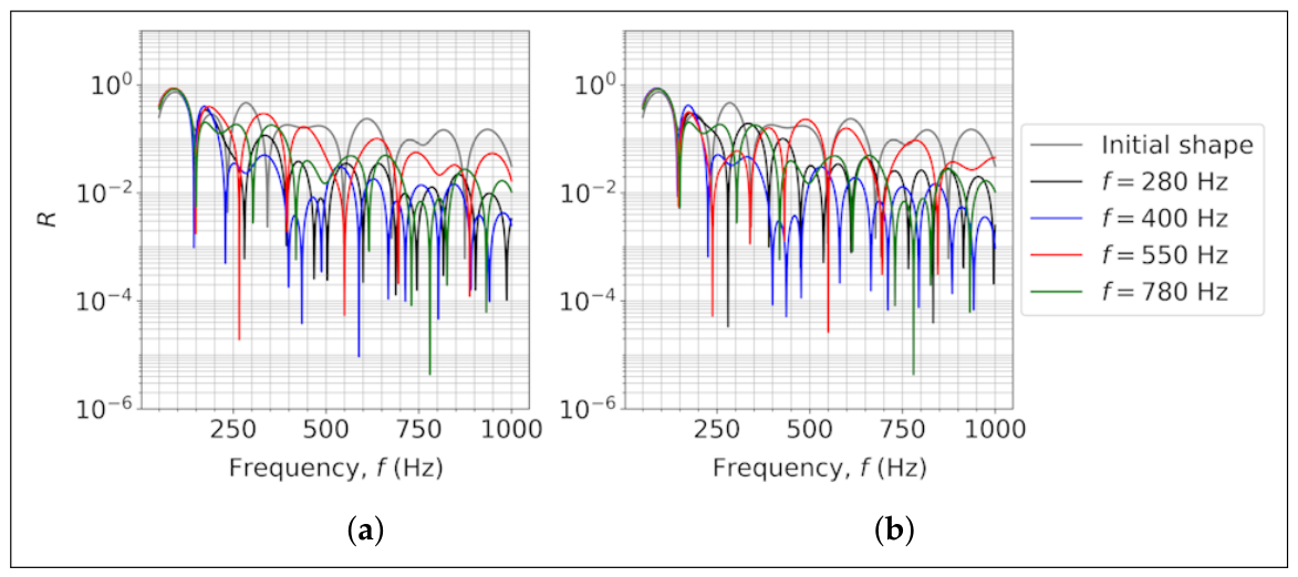
The objective function (J) was evaluated for each optimized geometry. Figure 11 shows the reflection spectra for the initial and optimized horn shapes, demonstrating a reduction in reflected energy across the frequency range.

The results confirm that the optimized horn shapes improve impedance matching, leading to lower reflections and better energy transmission. The open-source implementation in FEniCS [56] provides a transparent and accessible platform for shape optimization in acoustics.

4.2. Sound Barrier Optimization Results

The shape optimization framework was applied to the sound barrier problem to minimize the acoustic pressure levels in the shadow region behind the barrier. The optimization was performed at a frequency of 400 Hz, with different numbers of control points, N, ranging from $N=5$ to $N=20$.

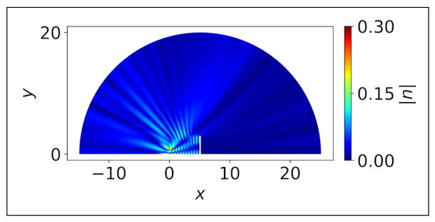
Figure 12 presents the sound pressure distribution for the initial straight barrier configuration. The goal of the optimization is to reshape the barrier’s front surface to enhance its noise-blocking performance by reducing diffraction effects and optimizing wave reflection.

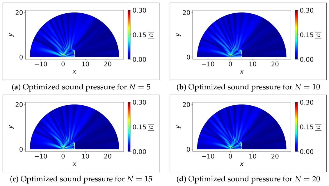
Figure 13 illustrates the optimized sound pressure distributions for different numbers of control points ($N=5,10,15,20$). The optimization process refines the barrier shape by introducing smooth curvature modifications that minimize the transmission of sound waves into the shadow zone.

The optimized barriers exhibit smoother curvatures at the upper edges, consistent with previous studies on acoustic barriers. Chen et al. [42] performed parametric shape optimization for absorbing material distribution, whereas Shaaban et al. [32] and Videla et al. [35] employed different optimization techniques to enhance barrier performance.

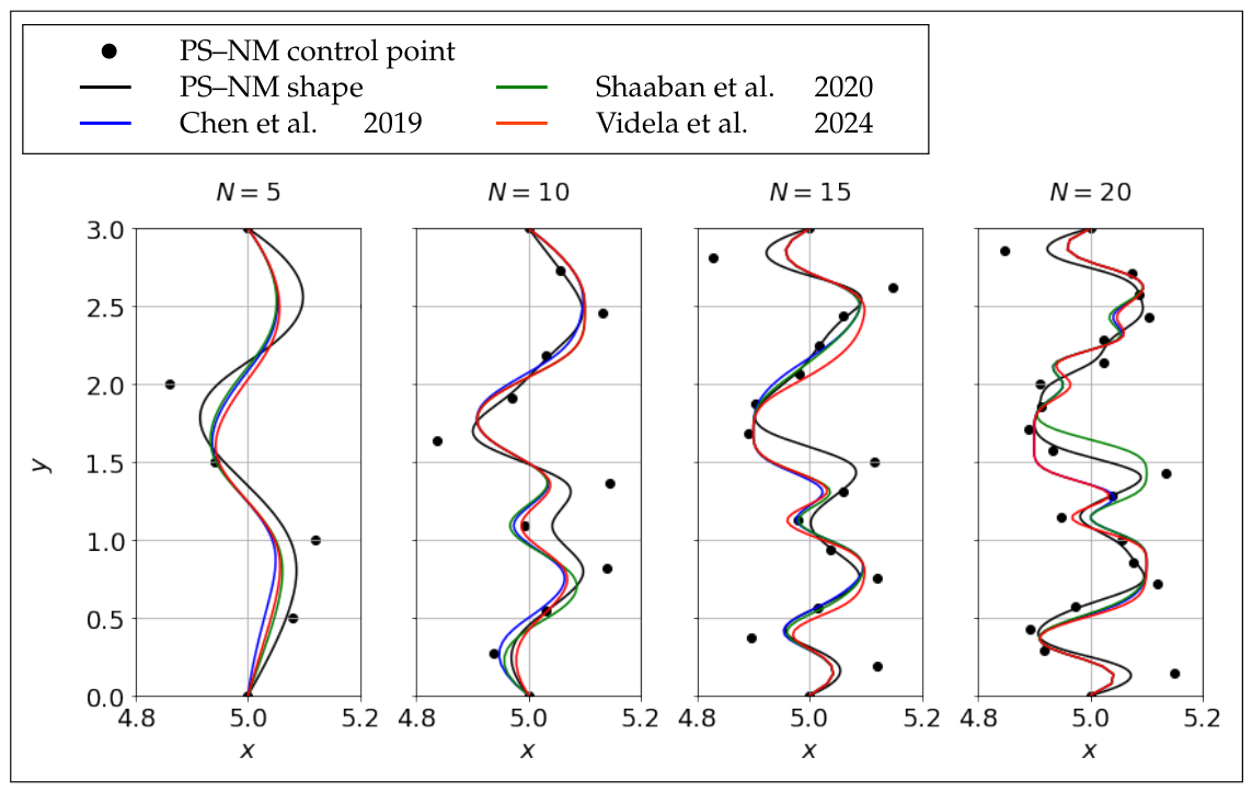
Figure 14 compares the optimized control points and barrier profiles obtained in this study with those reported by Chen et al. [42], Shaaban et al. [32], and Videla et al. [35]. This comparison should be interpreted qualitatively rather than as a one-to-one benchmark comparison. The compared studies use different objective functions, parameterizations, admissible design spaces, material assumptions, and constraint formulations. In particular, some previous studies optimize absorbing-material distributions or use different spline/control-point constraints, whereas the present study optimizes the front-face geometry of a rigid barrier under the area and feasibility restrictions described above. Therefore, the different optimized profiles may correspond to different admissible design spaces and different local minima of related but not identical optimization problems. The comparison is included to show that the proposed open-source workflow produces geometrically plausible optimized barrier profiles within the range of previously reported solutions, not to claim superiority over those methods. The present PS–NM optimization results are shown with black markers and lines.

The observed differences in the optimized barrier geometries therefore do not imply that one profile is universally superior to the others. Instead, they reflect the sensitivity of acoustic shape optimization to the admissible design space, objective definition, constraint set, and local basin of attraction. This interpretation is consistent with the non-convex nature of Helmholtz-based shape optimization and with the role of the PS stage as an initialization aid rather than a proof of global optimality.

Table 3. Optimization results for the barrier problem ($f=400$ Hz) using different number of control points N and two methods.

N	Method	DOF	${\mathit{n}}_{\mathbf{PS}}$	${\mathit{n}}_{\mathbf{NM}}$	t (s)	J	x-Coordinates of Points
5	1	230,197	-	69	1170.8	0.137805	$x_1$	$x_2$	$x_3$	$x_4$	$x_5$
							4.937	5.035	4.956	4.896	5.191
	2	233,983	126	62	2271.2	0.132054	$x_1$	$x_2$	$x_3$	$x_4$	$x_5$
							5.079	5.119	4.942	4.860	5.207
10	1	240,658	-	122	2214.0	0.120993	$x_1$	$x_2$	$x_3$	$x_4$	$x_5$
							5.006	4.989	5.139	4.986	5.142
							$x_6$	$x_7$	$x_8$	$x_9$	$x_{10}$
							4.826	5.005	4.998	5.153	5.024
	2	235,132	2212	144	22,816.8	0.118905	$x_1$	$x_2$	$x_3$	$x_4$	$x_5$
							4.937	5.030	5.139	4.992	5.144
							$x_6$	$x_7$	$x_8$	$x_9$	$x_{10}$
							4.836	4.971	5.030	5.132	5.055
15	1	243,316	-	199	3362.0	0.104444	$x_1$	$x_2$	$x_3$	$x_4$	$x_5$
							5.134	4.939	4.968	5.126	5.072
							$x_6$	$x_7$	$x_8$	$x_9$	$x_{10}$
							4.841	5.052	5.127	4.941	4.879
							$x_{11}$	$x_{12}$	$x_{13}$	$x_{14}$	$x_{15}$
							4.971	5.029	5.089	5.117	4.858
	2	239,320	3302	232	33,776.5	0.103223	$x_1$	$x_2$	$x_3$	$x_4$	$x_5$
							5.121	4.896	5.014	5.120	5.036
							$x_6$	$x_7$	$x_8$	$x_9$	$x_{10}$
							4.980	5.060	5.115	4.890	4.903
							$x_{11}$	$x_{12}$	$x_{13}$	$x_{14}$	$x_{15}$
							4.981	5.017	5.059	5.147	4.829
20	1	243,577	-	311	4977.2	0.097025	$x_1$	$x_2$	$x_3$	$x_4$	$x_5$
							5.208	4.853	4.965	4.959	5.105
							$x_6$	$x_7$	$x_8$	$x_9$	$x_{10}$
							5.085	5.005	5.050	5.044	5.101
							$x_{11}$	$x_{12}$	$x_{13}$	$x_{14}$	$x_{15}$
							4.944	5.010	4.983	4.961	4.982
							$x_{16}$	$x_{17}$	$x_{18}$	$x_{19}$	$x_{20}$
							5.049	5.096	5.065	5.122	4.813
	2	240,694	4421	262	45,446.0	0.094861	$x_1$	$x_2$	$x_3$	$x_4$	$x_5$
							5.148	4.917	4.893	4.973	5.119
							$x_6$	$x_7$	$x_8$	$x_9$	$x_{10}$
							5.076	5.056	4.949	5.039	5.134
							$x_{11}$	$x_{12}$	$x_{13}$	$x_{14}$	$x_{15}$
							4.933	4.891	4.913	4.910	5.023
							$x_{16}$	$x_{17}$	$x_{18}$	$x_{19}$	$x_{20}$
							5.023	5.103	5.087	5.074	4.847

presents the barrier optimization results at $f=400$ Hz for different numbers of control points N. As expected, increasing N provided greater geometric flexibility and systematically reduced the objective value J. For Method 1 (baseline-initialized NM), J decreased from $1.38\times {10}^{-1}$ at $N=5$ to $9.70\times {10}^{-2}$ at $N=20$, reflecting the benefit of finer parameterization. Method 2 achieved further reductions, with $J=9.49\times {10}^{-2}$ at $N=20$, consistently but modestly outperforming Method 1 across all tested values of N.

The relative reductions produced by Method 2 with respect to Method 1 are approximately 4.2%, 1.7%, 1.2%, and 2.2% for $N=5,10,15$, and 20, respectively. Therefore, the barrier results should not be interpreted as a large physical improvement in barrier performance. Rather, they show that PS-initialized local refinement can find slightly better feasible designs than baseline-initialized NM, while the dominant improvement in this example comes from increasing the number of geometric design variables. Because J is an integrated pressure-magnitude objective rather than a direct sound-pressure-level or insertion-loss metric, the practical acoustic significance of these small reductions requires further application-specific interpretation.

This improvement came at a significant computational cost: Method 2 required thousands of PS evaluations in addition to NM iterations, leading to runtimes an order of magnitude longer than those of Method 1. For instance, at $N=20$, the runtime increased from approximately 5000 s (Method 1) to over 45,000 s (Method 2). The growth in runtime is attributed both to the larger number of design variables and to the exponential increase in possible PS configurations.

The optimized control-point coordinates produce modest but systematic modifications of the spline-generated barrier front face. Small forward and backward variations in the auxiliary control points lead to a slightly serrated evaluated profile, which can modify diffraction and slightly lower the integrated acoustic pressure in the shadow zone. These changes are consistent with barrier optimization studies in the literature and confirm that the PS–NM workflow can exploit additional design freedom while maintaining feasible geometries.

Overall, the barrier results highlight the central trade-off of the proposed approach: Method 2 gives modest objective-function reductions for this example, but at substantially higher computational cost as the dimensionality of the design space increases.

The objective function (J), representing the integrated acoustic pressure magnitude in the shadow region, was evaluated for each optimized barrier shape. The results indicate that increasing the number of control points improves the objective value by enabling more refined shape adjustments. However, since the additional improvement produced by Method 2 is small for this benchmark, these findings should be interpreted as evidence of improved numerical search robustness rather than as a definitive claim of large practical noise-reduction gains.

4.3. Crescent Optimization Results

The shape optimization framework was applied to the crescent-shaped scatterer problem for three different wavenumbers: $k=5$, $k=10$, and $k=15$. The analysis was conducted using both Parameter Sweep (PS) and the two-stage PS–NM workflow to determine the optimized geometries for minimizing the acoustic pressure in the shadow zone.

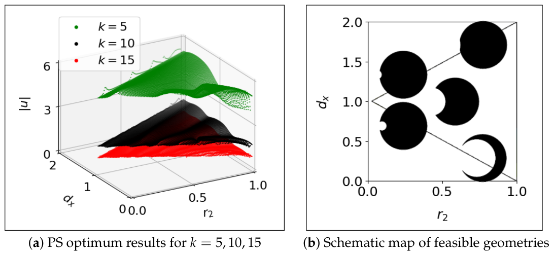
Figure 15a illustrates the optimization results obtained via parameter sweep within the feasible design space for each wavenumber. Figure 15b provides a schematic map of the feasible geometries, allowing for a clearer understanding of the range of possible designs.

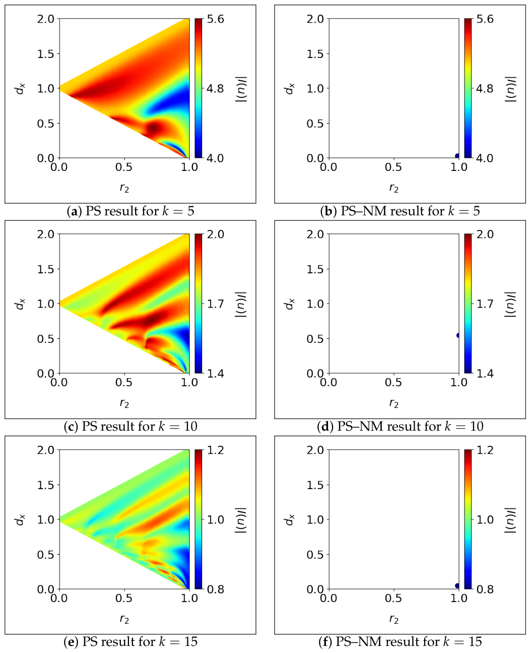
For lower wavenumbers, the wavelength is longer, leading to a broader spatial distribution of the acoustic field across the feasible solution space. The triangular clusters observed in Figure 15a represent different energy levels in the feasible region. To analyze these distributions further, Figure 16 presents detailed comparisons of PS and PS–NM optimization results for each wavenumber.

The results indicate that the optimal solutions obtained with PS and PS–NM refinement are closely aligned, confirming the consistency of the optimization framework. The clustering of optimal values within the feasible region (Figure 16) suggests the presence of multiple locally optimal solutions with similar performance. This robustness in the solution space indicates that the geometry is sensitive to minor perturbations but the optimization method still maintains its effectiveness.

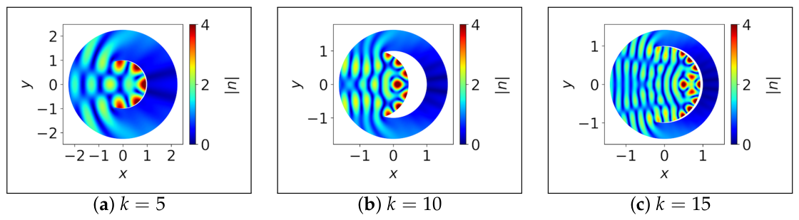
The sound pressure distributions for the optimized crescent geometries are shown in Figure 17. For each case, high-amplitude pressure zones appear along the inner curvature of the crescent. These focal points of energy create a secondary scattering wavefront, effectively reducing the acoustic pressure in the downstream region.

Table 4. Optimization results for crescent-shaped scatterer problem.

k	Method	DOF	${\mathit{n}}_{\mathbf{PS}}$	${\mathit{n}}_{\mathbf{NM}}$	Time (s)	J	${\mathit{r}}_2$	${\mathit{d}}_{\mathit{x}}$
5	1	79,818	–	13	19.2134	5.08898	1.00	1.999
	2	97,215	10,000	10	18,858.1	4.01324	0.99	0.031
10	1	127,527	–	15	34.4323	1.80369	1.00	1.998
	2	175,062	10,000	21	34,051.8	1.42364	1.00	0.545
15	1	173,682	–	15	49.6906	1.01337	1.00	1.998
	2	333,174	10,000	55	57,841.9	0.789113	0.99	0.053

presents the optimization results for the crescent-shaped scatterer at wavenumbers $k=5$, 10, and 15. In all cases, Method 2 achieved lower objective values than Method 1 (baseline-initialized NM). For example, at $k=15$, the objective function was reduced from $J=1.01$ (Method 1) to $J=0.79$ (Method 2), corresponding to a 22% reduction in the integrated downstream pressure-magnitude objective. Similar reductions are observed at $k=5$ and $k=10$, demonstrating that PS initialization can improve local-refinement performance for this two-parameter scattering problem.

The trade-off is again visible in the computational cost. Each Method 2 run required $10,000$ PS evaluations in addition to NM iterations, leading to runtimes exceeding 18,000 s at $k=5$ and nearly 58,000 s at $k=15$, compared to less than 50 s for Method 1. This highlights the steep increase in runtime when a dense PS grid is combined with repeated FEM solutions, even for a two-variable design space.

The optimized geometric parameters illustrate how the crescent shape enhances acoustic performance. Under Method 1, the secondary cylinder radius $r_2$ and offset $d_x$ remain essentially unchanged from the initial offset configuration, resulting in limited scattering modification. In contrast, Method 2 identifies offsets on the order of $d_x\approx 0.05$–$0.55$, creating an asymmetric cavity that produces secondary scattering and improves wave cancellation in the shadow region. This demonstrates the importance of systematic global exploration (via PS) in identifying frequency-dependent scattering configurations that local optimization alone may fail to reach.

The optimized offset distance $d_x$ does not vary monotonically with wavenumber. Instead, the results suggest that the preferred crescent geometry depends on the interaction between wavelength, cavity opening, and the downstream integration region. For $k=5$ and $k=15$, the PS-initialized strategy identifies compact crescent configurations with small offsets, whereas for $k=10$ it identifies a more open asymmetric configuration. This indicates that the optimization landscape contains multiple frequency-dependent local optima rather than a simple monotonic trend with respect to k.

Both PS and PS–NM refinement yield consistent results, identifying multiple local optima with comparable objective function values. The crescent shape effectively scatters acoustic waves, with inner curvature reflections forming secondary wavefronts. The optimized geometries vary non-monotonically with k, indicating a frequency-dependent scattering effect governed by the interaction between wavelength and crescent geometry.

These findings indicate that the crescent-shaped scatterer can serve as an effective structure for acoustic wave redirection and attenuation, with performance strongly influenced by the incident wave frequency.

5. Methodological Limitations and Computational-Budget Dependence

The numerical results reported in this study depend on the selected design parameterization, parameter bounds, PS resolution or random-sampling budget, mesh resolution, and NM stopping tolerances. The PS stage improves the initialization of the local optimizer, but it does not eliminate the possibility that untested regions of the design space contain better feasible designs. A finer PS discretization may improve the initial candidate supplied to NM, but it also increases the number of FEM solves and the wall-clock time. This trade-off is visible in the reported values of $n_{\mathrm{PS}}$ and runtime, particularly for the sound-barrier and crescent examples.

For the high-dimensional barrier cases, the random sampling used when $C>{10}^4$ should therefore be viewed as a computational-budget-limited screening step. It provides a practical way to generate feasible starting points when exhaustive enumeration is prohibitive, but it does not provide a formal coverage guarantee. A systematic PS-resolution sensitivity study over all benchmark cases would require a large number of additional FEM solves and is left as a natural extension of the present work. The present results should consequently be interpreted as the best solutions found within the specified computational budget, rather than as PS-resolution-independent optima.

6. Conclusions

This study presented an open-source two-stage PS–NM workflow for acoustic shape optimization, demonstrated on three benchmark cases: an acoustic horn, a sound barrier, and a crescent-shaped scatterer. The workflow combines a Parameter Sweep (PS) method for feasibility exploration and candidate selection with penalty-augmented Nelder–Mead local refinement. The contribution is not a new abstract optimization algorithm, but a reproducible end-to-end implementation that integrates geometry generation, finite element Helmholtz analysis, absorbing boundary treatment, feasibility screening, and derivative-free local refinement in a FEniCS/Jupyter environment.

For the acoustic horn, the optimized geometries improved impedance matching and reduced reflections, with results consistent with previous studies. The large improvement over baseline-initialized NM illustrates the sensitivity of Helmholtz shape optimization to local basins of attraction and the benefit of PS-based initialization. In the sound barrier problem, increasing the number of control points reduced the integrated pressure-magnitude objective in the shadow region. The additional improvement produced by PS initialization was consistent but modest, and should therefore be interpreted cautiously in terms of practical acoustic significance. The crescent scatterer introduced a cavity-inspired scattering geometry, where optimization revealed secondary scattering effects that reduced the downstream pressure-magnitude objective.

The reported designs are not claimed to be unique or globally optimal. They are the best solutions obtained within the prescribed finite-dimensional parameterizations, geometric constraints, mesh resolution, PS resolution or sampling budget, and NM stopping tolerances. The implementation in FEniCS 2019.1.0 within a Jupyter Notebook 6.0.2 environment underscores the advantages of transparency and reproducibility, providing an accessible alternative to proprietary optimization workflows. Future extensions may include adaptive or constraint-aware penalty strategies, systematic PS-resolution studies, multi-objective formulations, frequency-adaptive designs, and integration with metamaterial concepts.

In summary, the results demonstrate that open-source, reproducible optimization workflows can provide a useful and flexible platform for computational acoustic shape optimization, while making the accuracy–cost and initialization-sensitivity trade-offs explicit.