Figure 1.
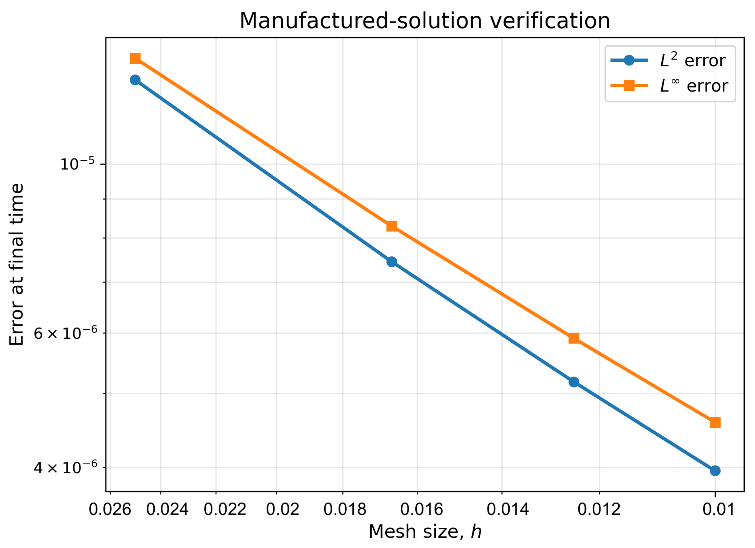
Manufactured-solution verification. The final-time and errors decrease under coupled mesh and time-step refinement, confirming the convergence of the implemented fractional-memory, nonlinear-flux, and Robin-boundary discretization.
Figure 1.
Manufactured-solution verification. The final-time and errors decrease under coupled mesh and time-step refinement, confirming the convergence of the implemented fractional-memory, nonlinear-flux, and Robin-boundary discretization.
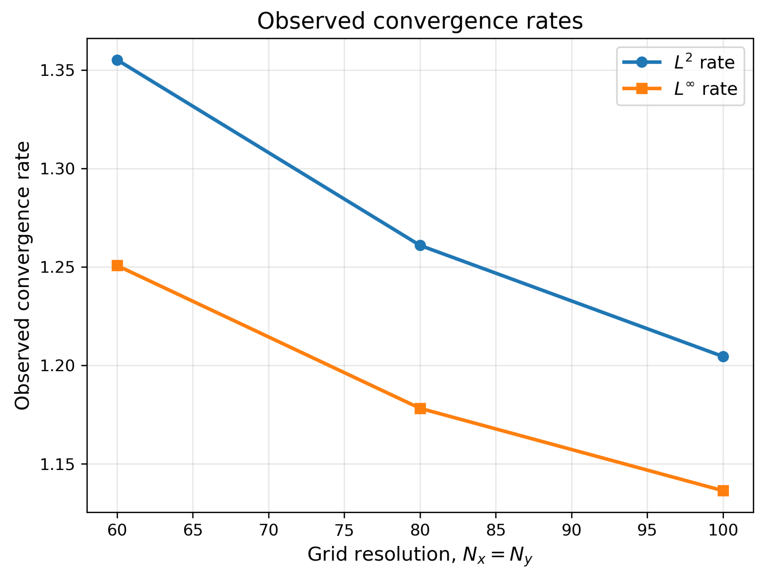
Figure 2.
Observed convergence rates for the manufactured-solution verification. The rates remain positive over all refinements and reflect the combined effects of L1 fractional memory, nonlinear coefficient freezing, Robin boundary-row replacement, and heterogeneous flux discretization.
Figure 2.
Observed convergence rates for the manufactured-solution verification. The rates remain positive over all refinements and reflect the combined effects of L1 fractional memory, nonlinear coefficient freezing, Robin boundary-row replacement, and heterogeneous flux discretization.
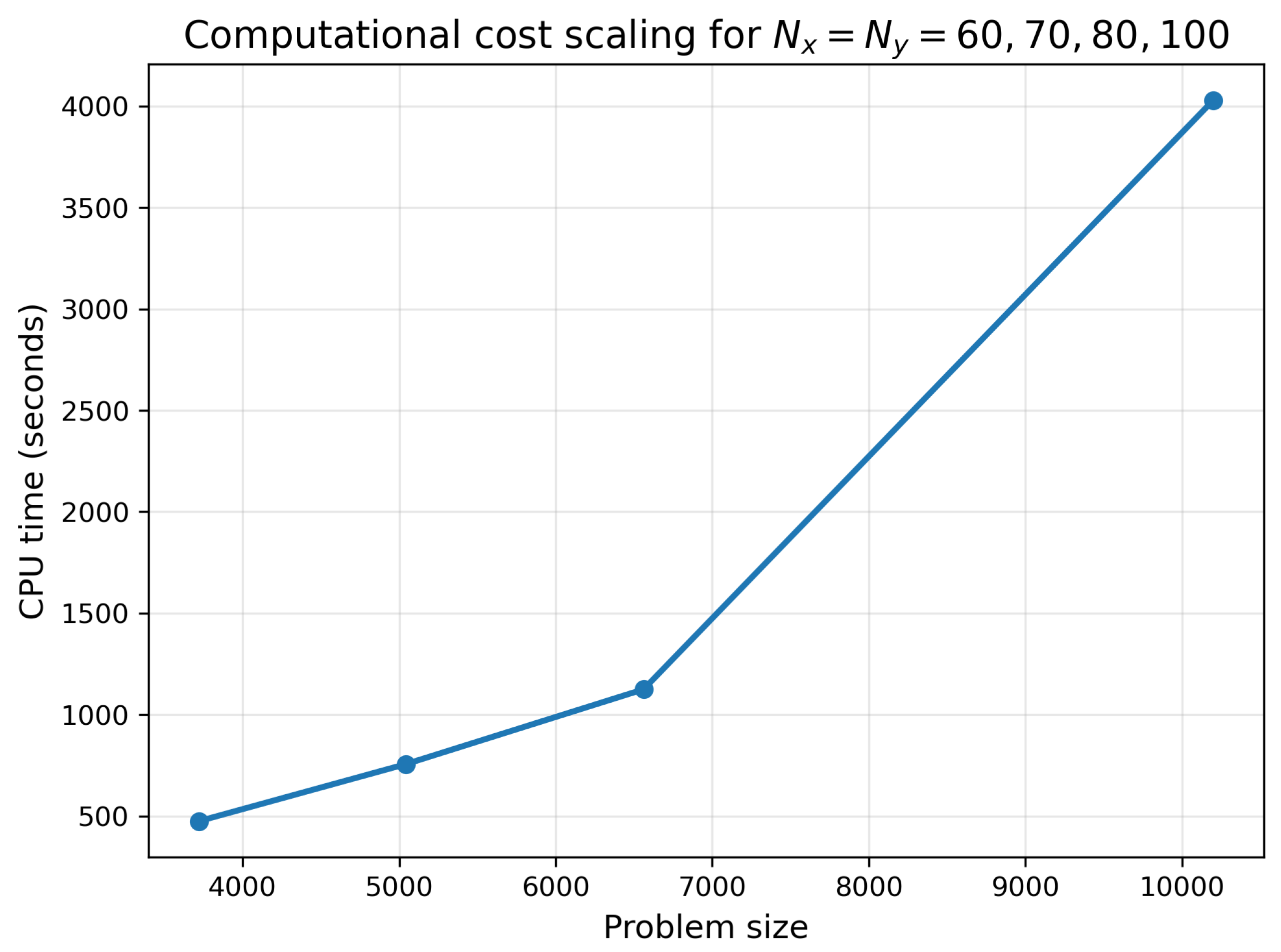
Figure 3.
Computational cost scaling for . The increase in CPU time reflects the larger sparse systems, longer fractional histories, and repeated Picard solves.
Figure 3.
Computational cost scaling for . The increase in CPU time reflects the larger sparse systems, longer fractional histories, and repeated Picard solves.
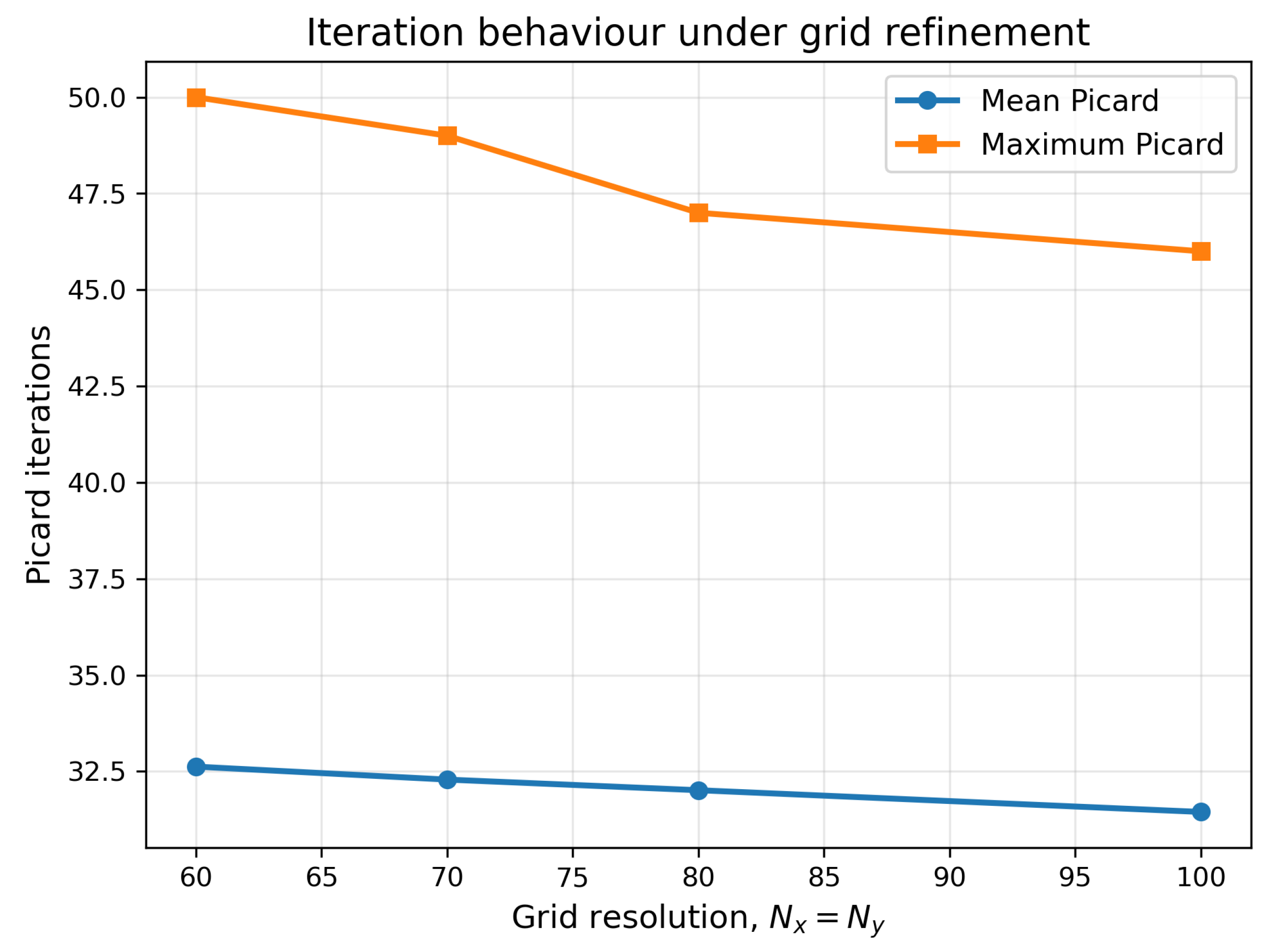
Figure 4.
Picard iteration behavior under grid refinement. The mean and maximum Picard iteration counts remain bounded as the grid is refined, indicating stable nonlinear iteration behavior.
Figure 4.
Picard iteration behavior under grid refinement. The mean and maximum Picard iteration counts remain bounded as the grid is refined, indicating stable nonlinear iteration behavior.
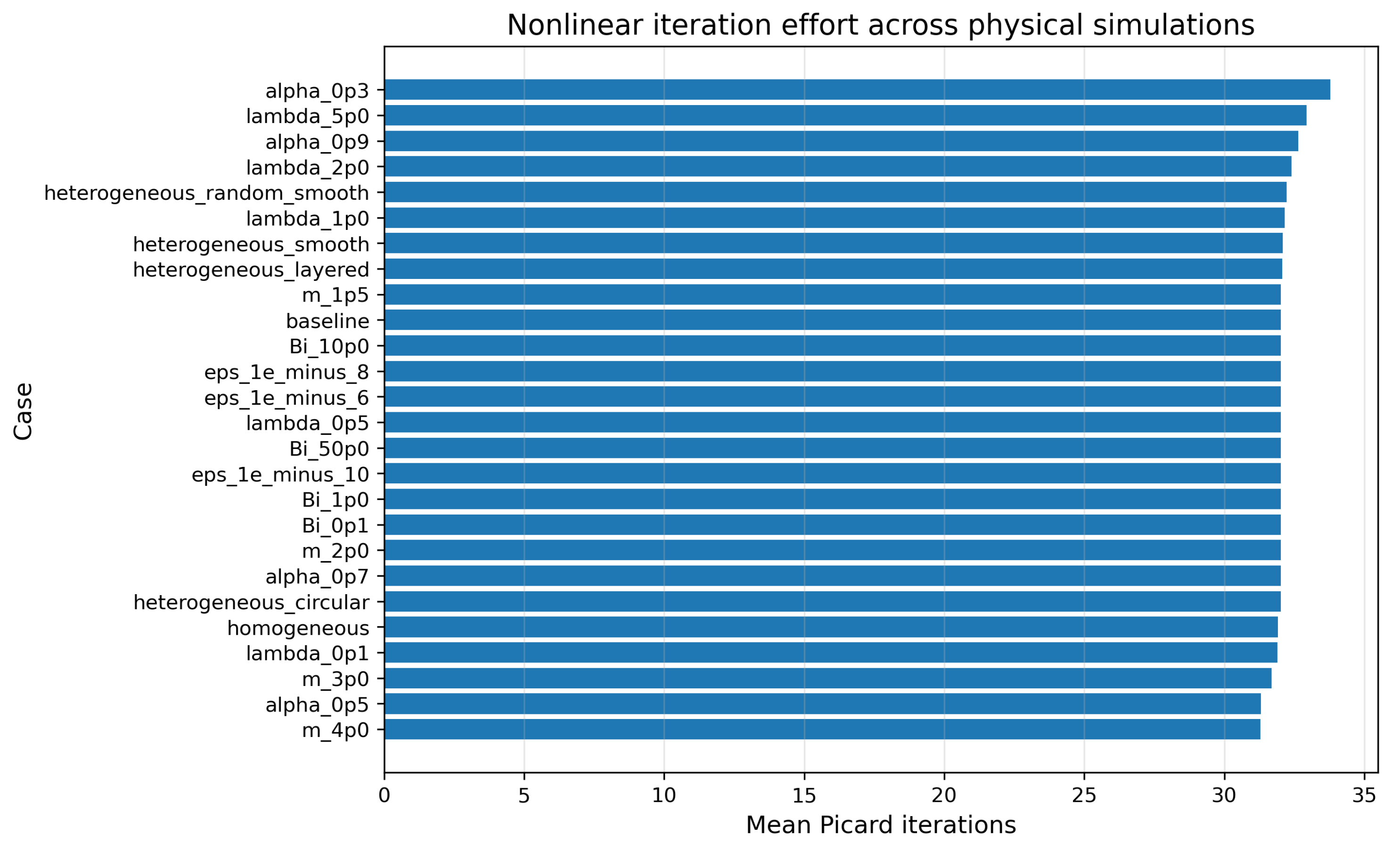
Figure 5.
Mean Picard iteration effort across the physical simulations. Strong memory and strong forcing require slightly larger nonlinear effort, but no solver breakdown is observed.
Figure 5.
Mean Picard iteration effort across the physical simulations. Strong memory and strong forcing require slightly larger nonlinear effort, but no solver breakdown is observed.
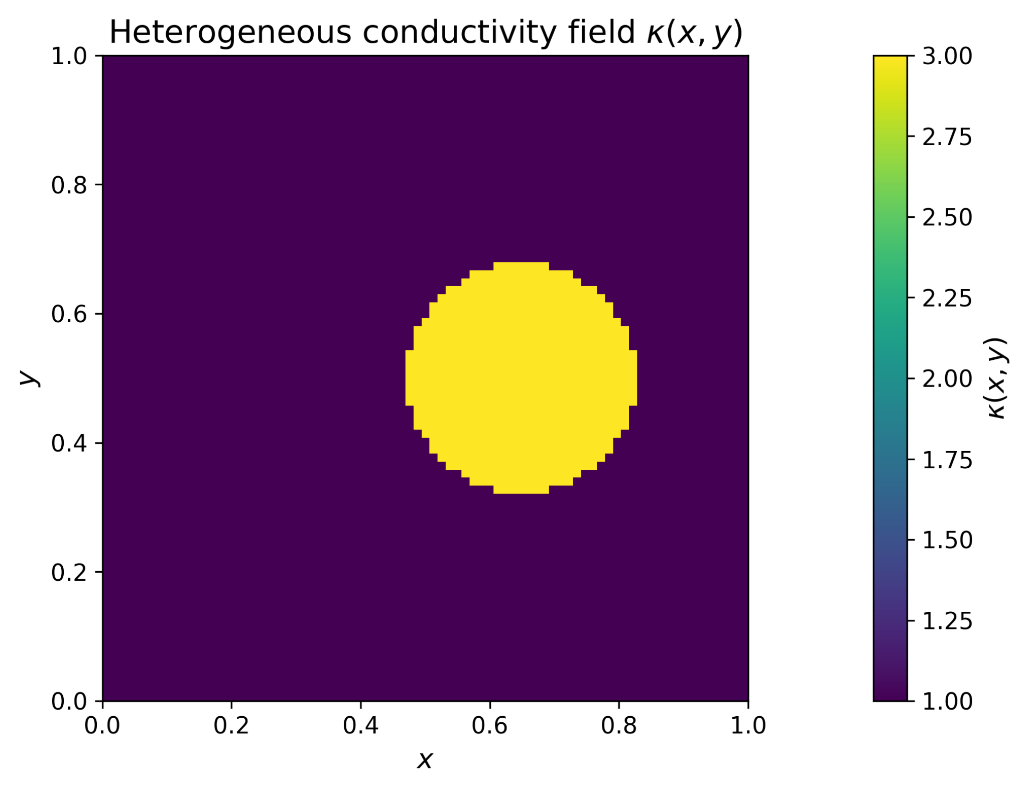
Figure 6.
Reference heterogeneous conductivity field . The background medium has , while the circular inclusion has . The inclusion modifies the diffusive flux without acting as an additional heat source.
Figure 6.
Reference heterogeneous conductivity field . The background medium has , while the circular inclusion has . The inclusion modifies the diffusive flux without acting as an additional heat source.
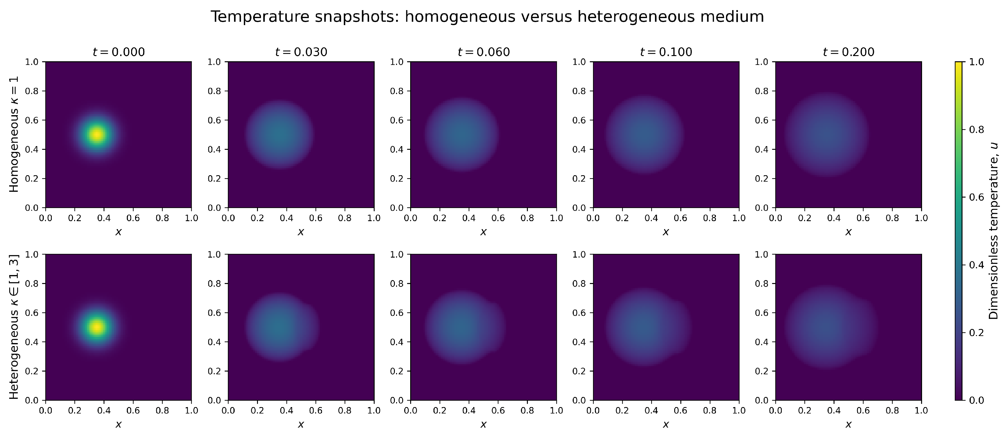
Figure 7.
Temperature snapshots comparing homogeneous and circular heterogeneous media at , , , and . The homogeneous case remains nearly symmetric, whereas the heterogeneous case develops front deformation and preferential redistribution towards the more conductive region.
Figure 7.
Temperature snapshots comparing homogeneous and circular heterogeneous media at , , , and . The homogeneous case remains nearly symmetric, whereas the heterogeneous case develops front deformation and preferential redistribution towards the more conductive region.
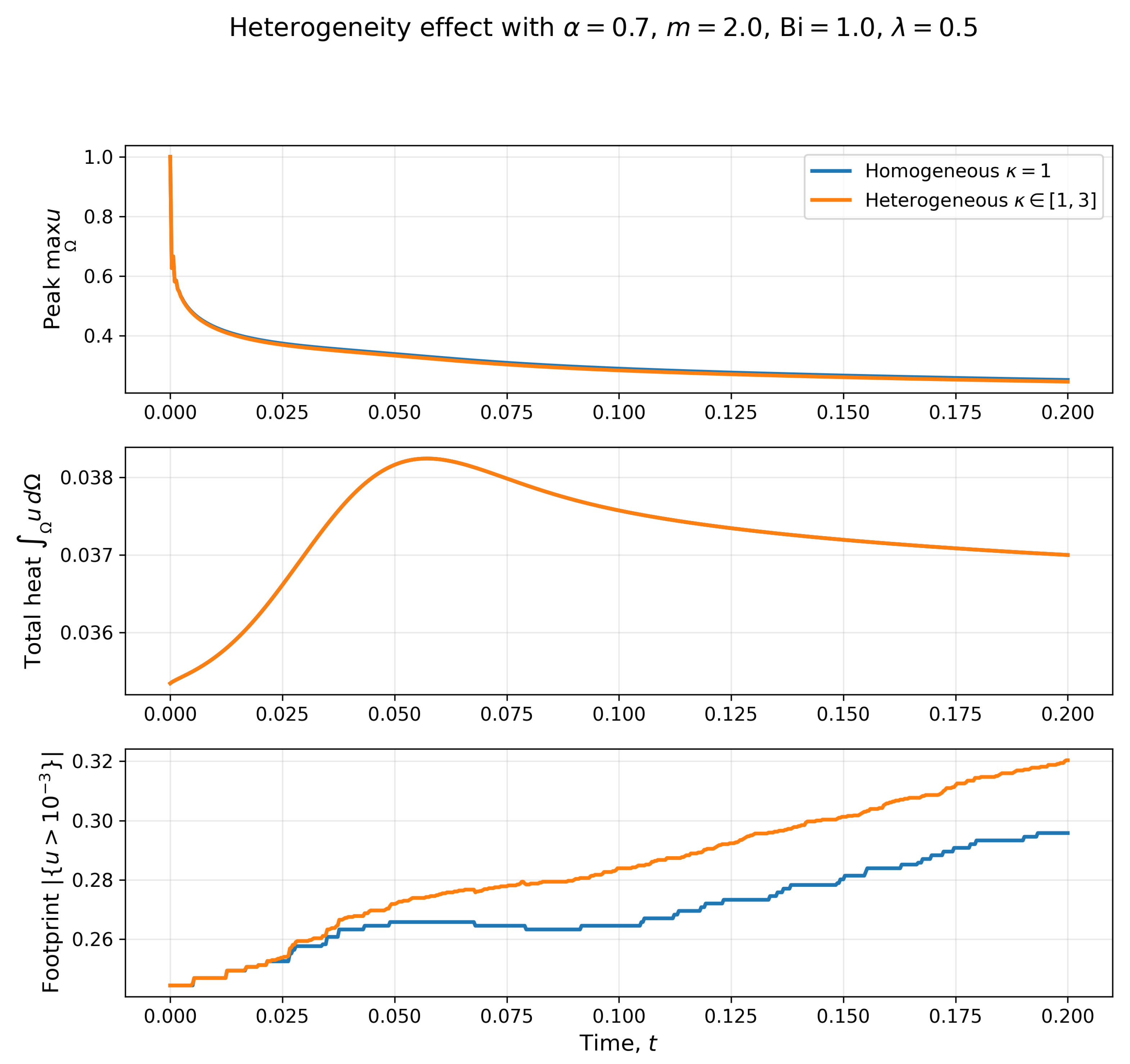
Figure 8.
Effect of material heterogeneity on peak temperature, total heat content, and thermal footprint. Heterogeneity modifies the footprint more strongly than the total heat content, indicating that its primary role is spatial redistribution.
Figure 8.
Effect of material heterogeneity on peak temperature, total heat content, and thermal footprint. Heterogeneity modifies the footprint more strongly than the total heat content, indicating that its primary role is spatial redistribution.
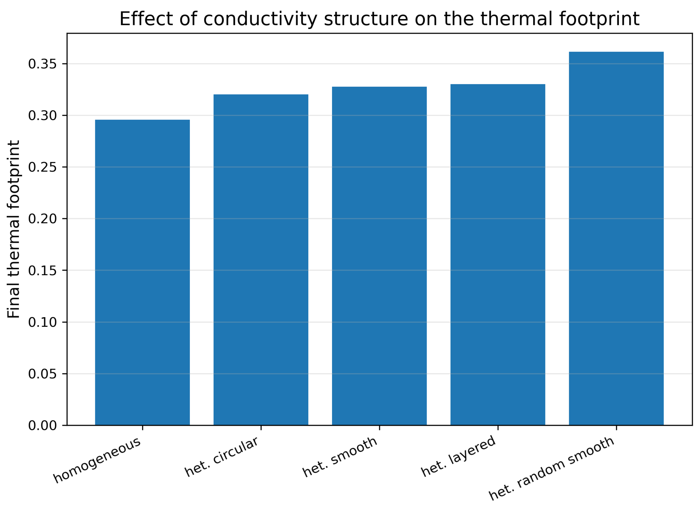
Figure 9.
Effect of conductivity structure on the final thermal footprint. Homogeneous, circular heterogeneous, smooth heterogeneous, layered, and random smooth fields are compared under the same physical parameters.
Figure 9.
Effect of conductivity structure on the final thermal footprint. Homogeneous, circular heterogeneous, smooth heterogeneous, layered, and random smooth fields are compared under the same physical parameters.
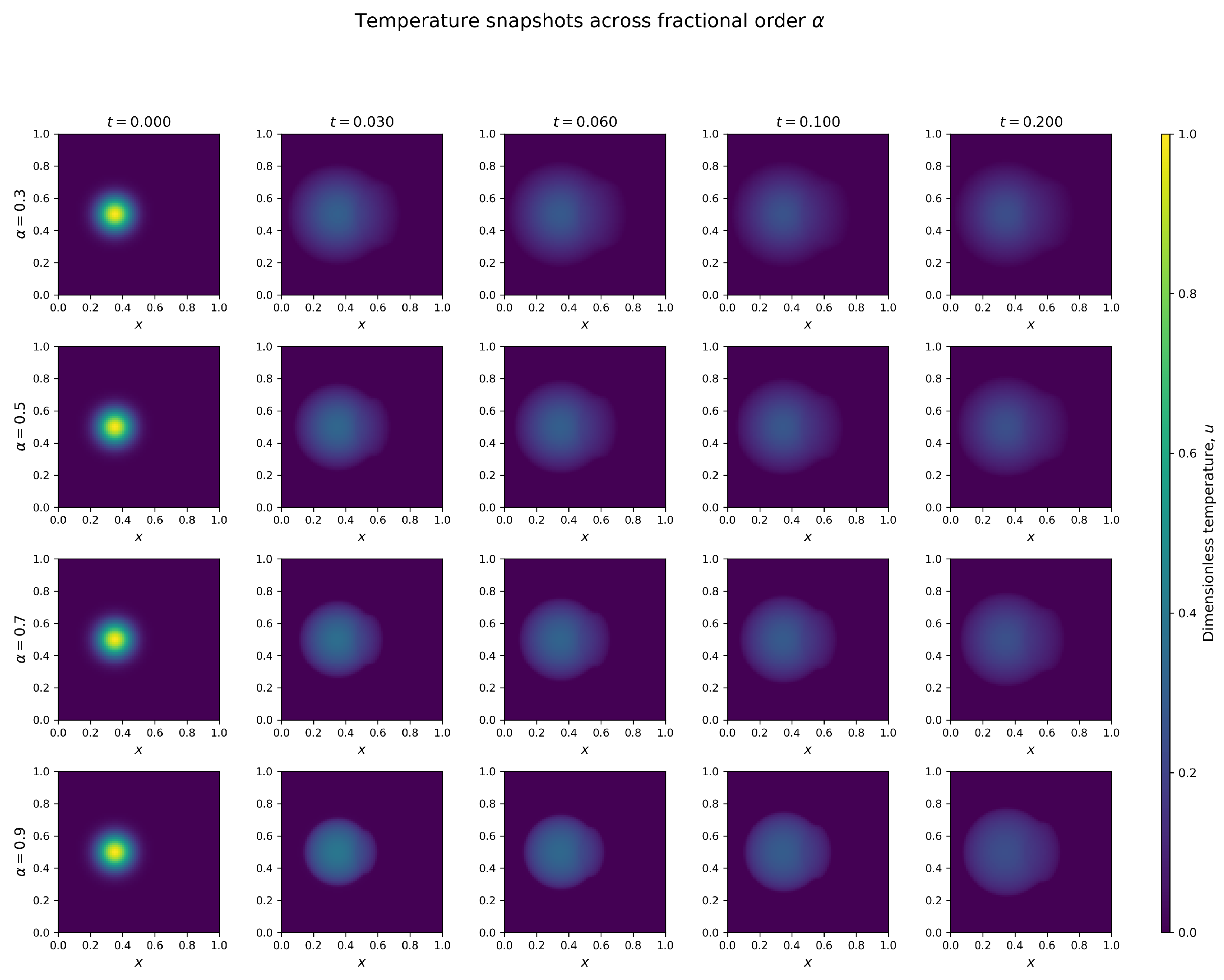
Figure 10.
Temperature snapshots across fractional order at fixed , , and . Smaller fractional orders generate broader and more persistent thermal regions.
Figure 10.
Temperature snapshots across fractional order at fixed , , and . Smaller fractional orders generate broader and more persistent thermal regions.
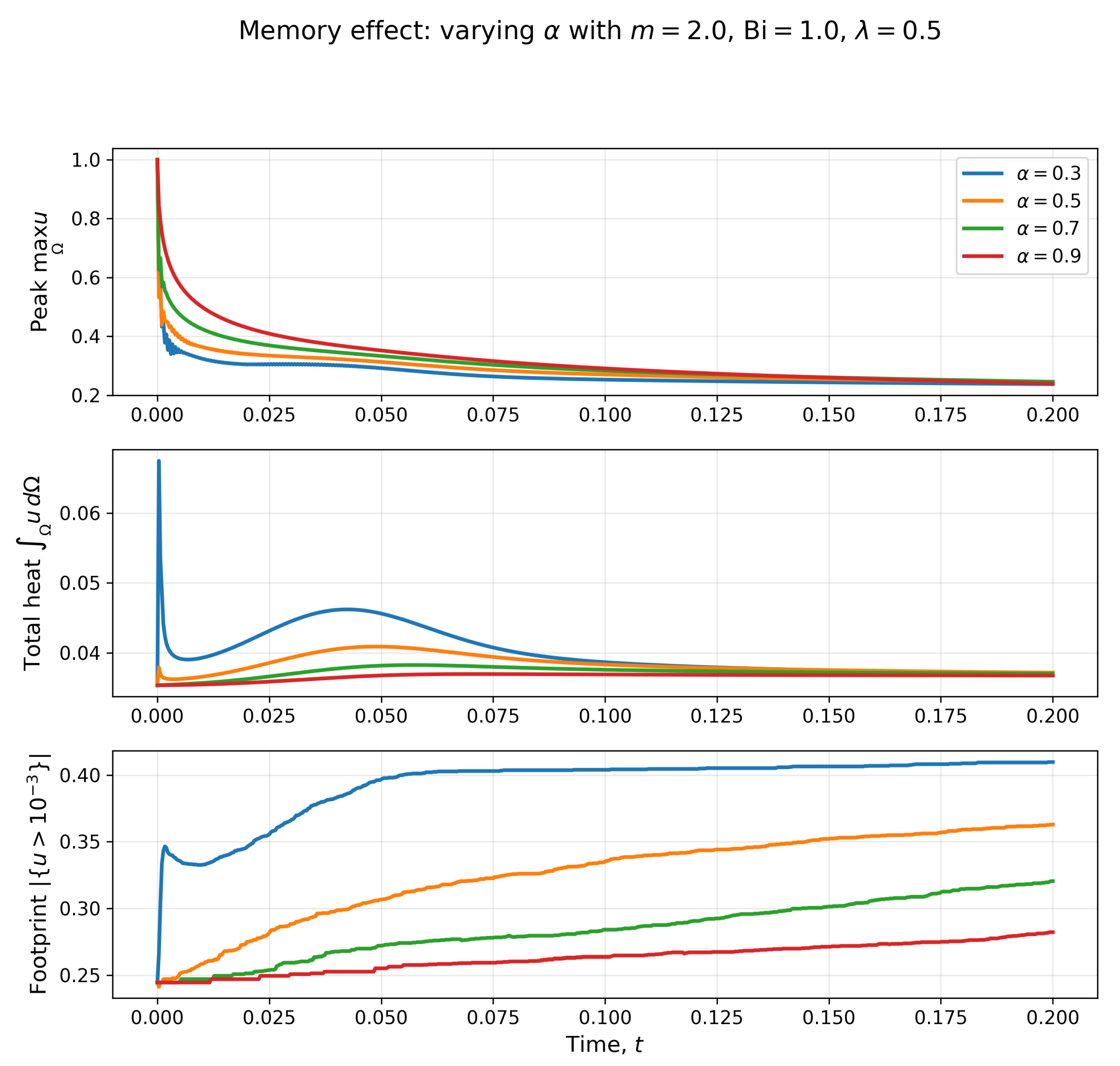
Figure 11.
Memory effect obtained by varying . The fractional order affects peak temperature, total heat content, and footprint in different ways, indicating that memory changes persistence rather than merely rescaling diffusion speed.
Figure 11.
Memory effect obtained by varying . The fractional order affects peak temperature, total heat content, and footprint in different ways, indicating that memory changes persistence rather than merely rescaling diffusion speed.
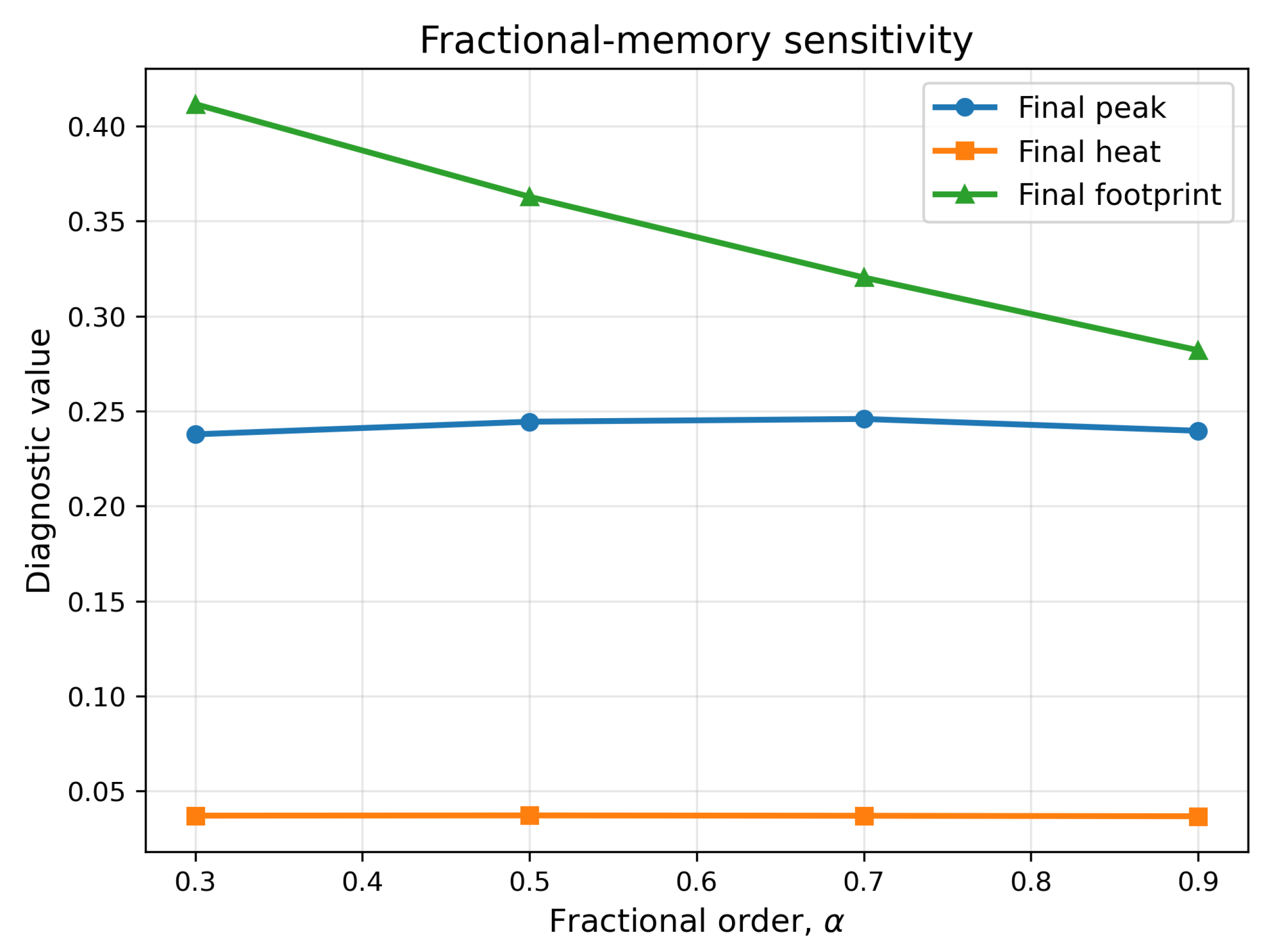
Figure 12.
Final diagnostic values across fractional order . Smaller produces a larger thermal footprint, while the final peak and heat content vary more moderately.
Figure 12.
Final diagnostic values across fractional order . Smaller produces a larger thermal footprint, while the final peak and heat content vary more moderately.
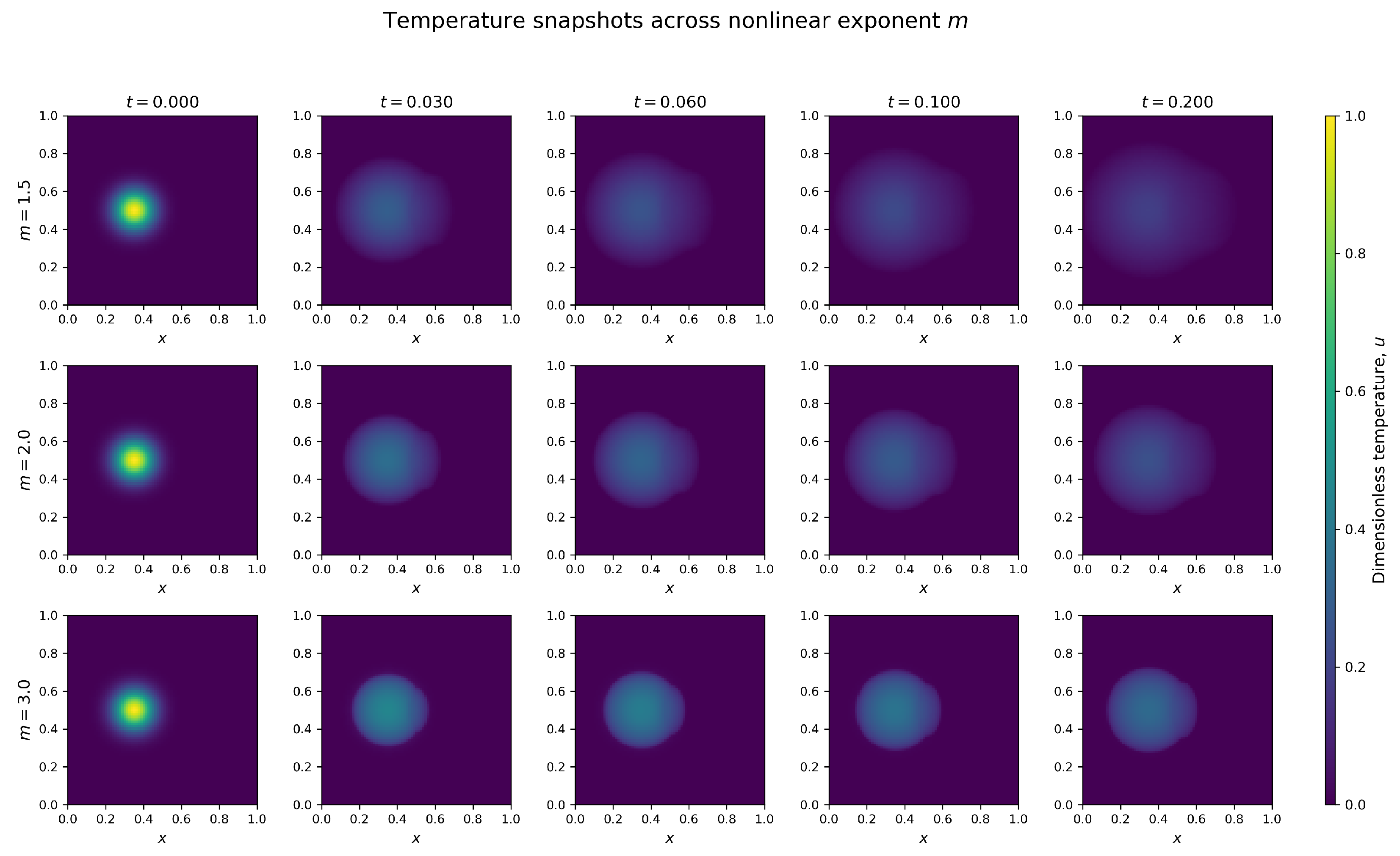
Figure 13.
Temperature snapshots across nonlinear exponent m at fixed , , and . Smaller m promotes spreading, whereas larger m confines heat near the source.
Figure 13.
Temperature snapshots across nonlinear exponent m at fixed , , and . Smaller m promotes spreading, whereas larger m confines heat near the source.
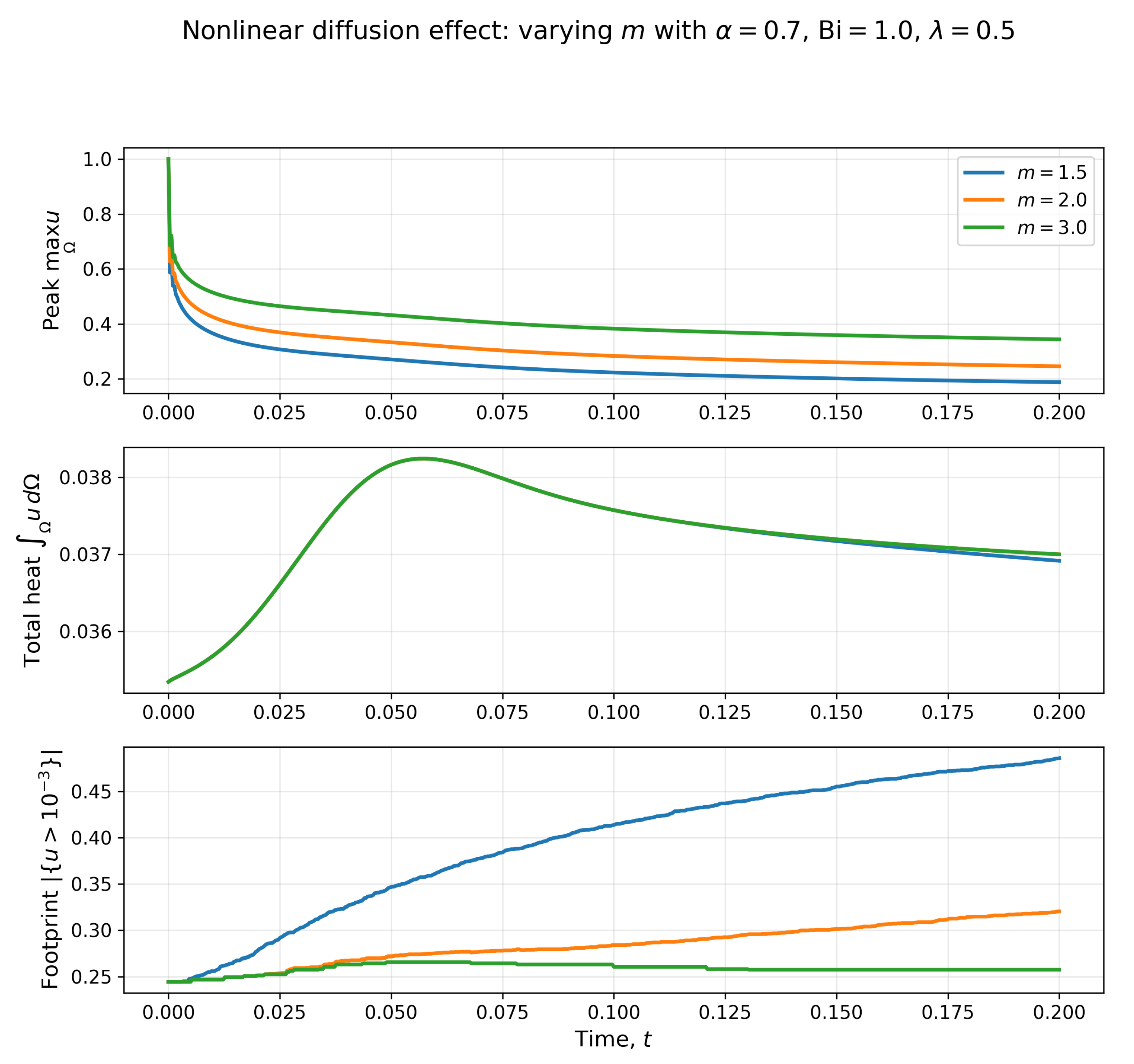
Figure 14.
Nonlinear-mobility effect obtained by varying m. Larger m increases peak temperature and reduces the footprint, indicating stronger localization.
Figure 14.
Nonlinear-mobility effect obtained by varying m. Larger m increases peak temperature and reduces the footprint, indicating stronger localization.
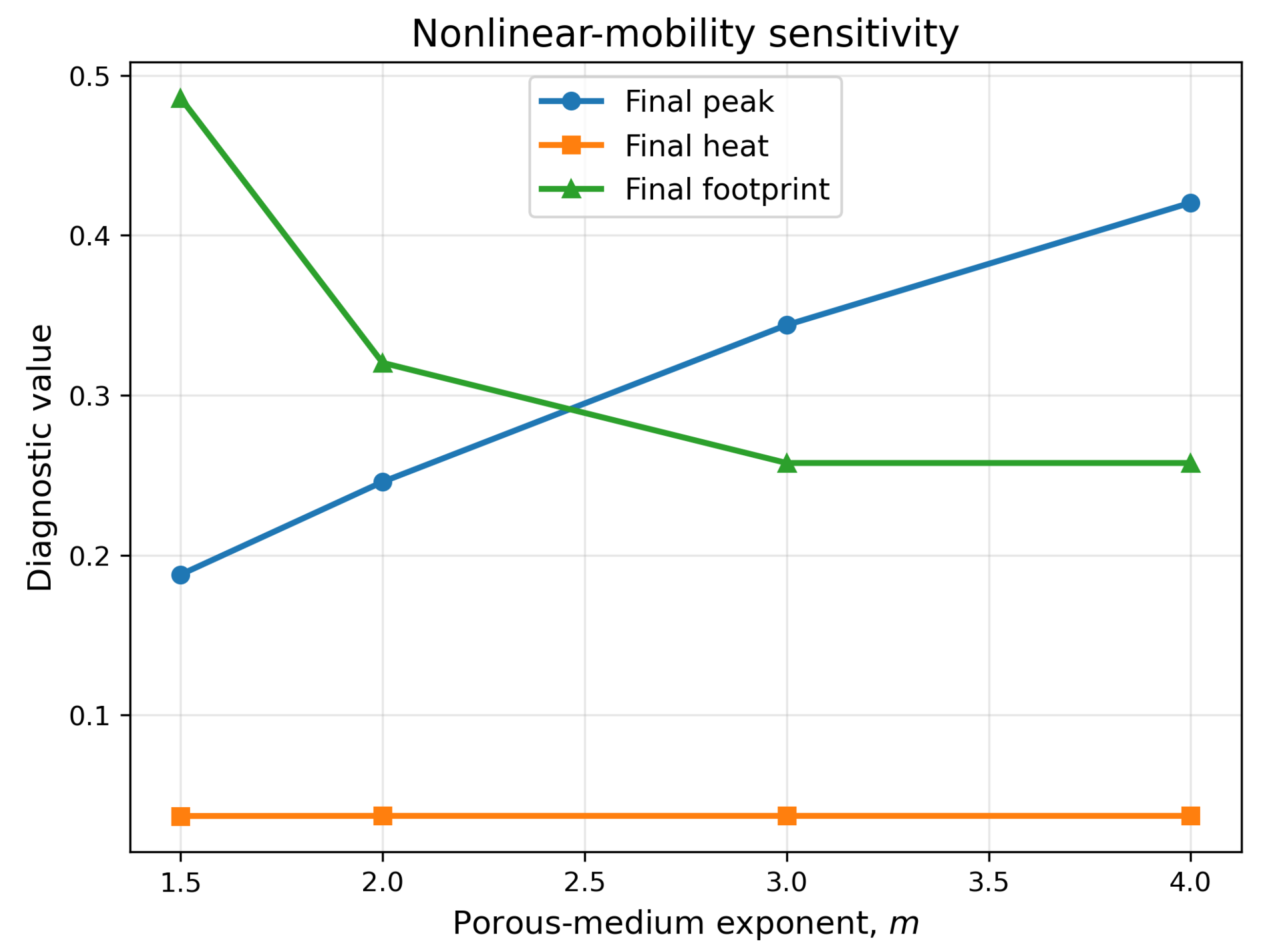
Figure 15.
Final diagnostic values across porous-medium exponent m. Increasing m raises the final peak and reduces the final footprint, while the final heat content remains almost unchanged.
Figure 15.
Final diagnostic values across porous-medium exponent m. Increasing m raises the final peak and reduces the final footprint, while the final heat content remains almost unchanged.
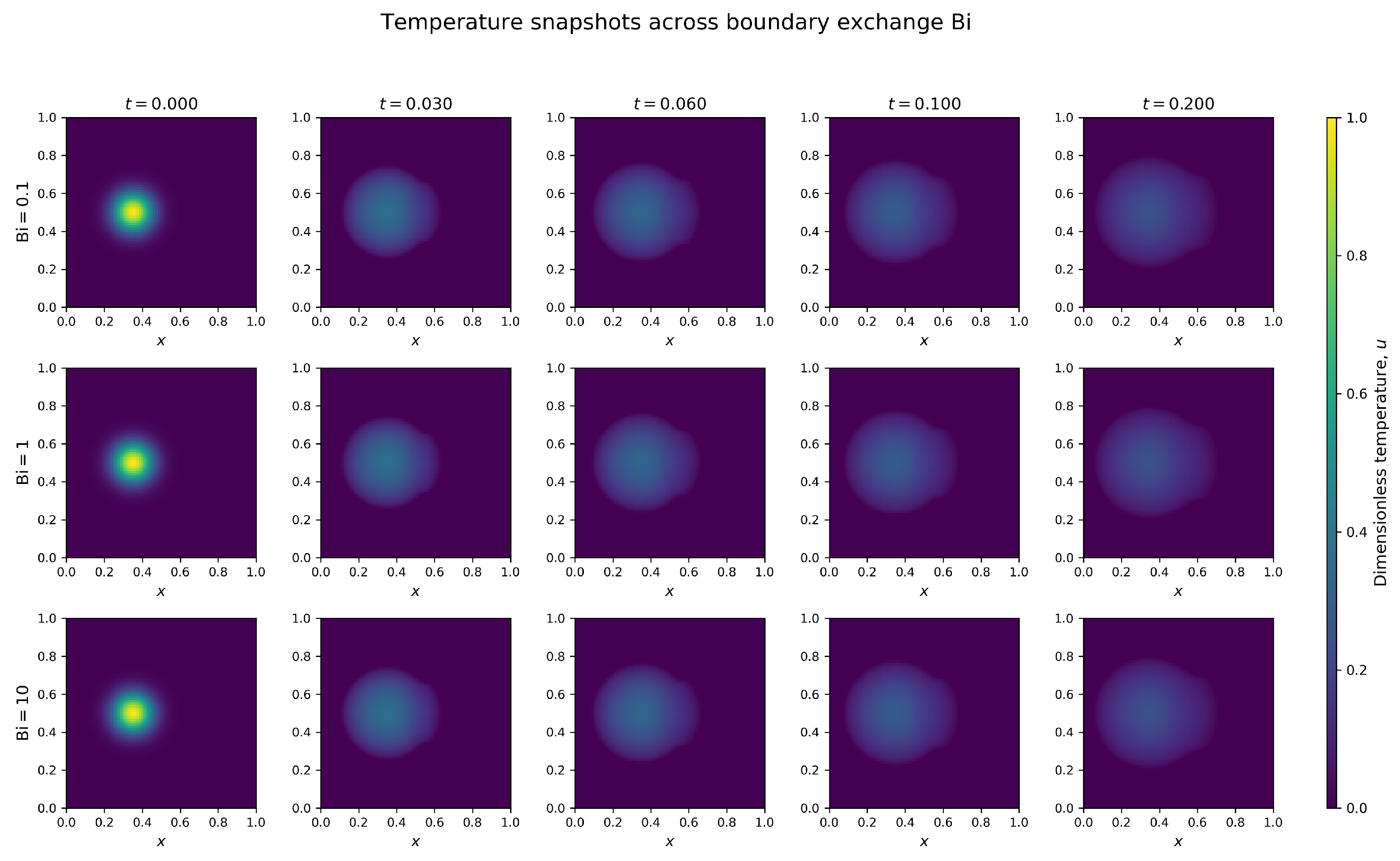
Figure 16.
Temperature snapshots across boundary exchange parameter at fixed , , and . The thermal fields remain nearly indistinguishable over the simulated interval.
Figure 16.
Temperature snapshots across boundary exchange parameter at fixed , , and . The thermal fields remain nearly indistinguishable over the simulated interval.
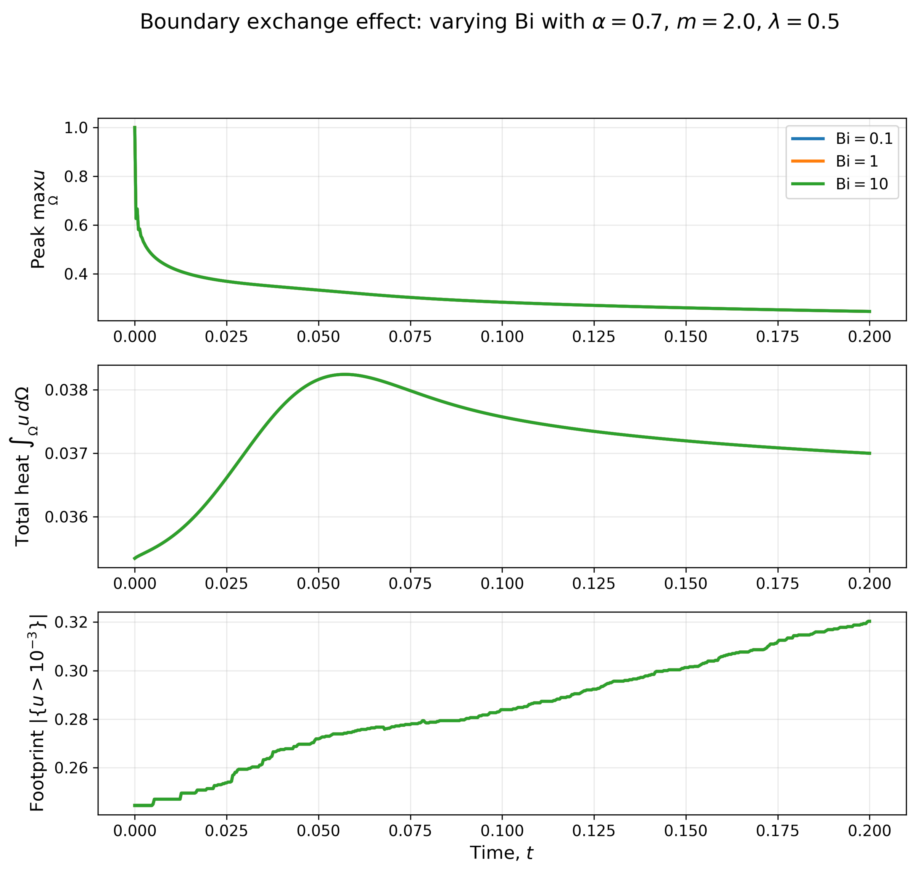
Figure 17.
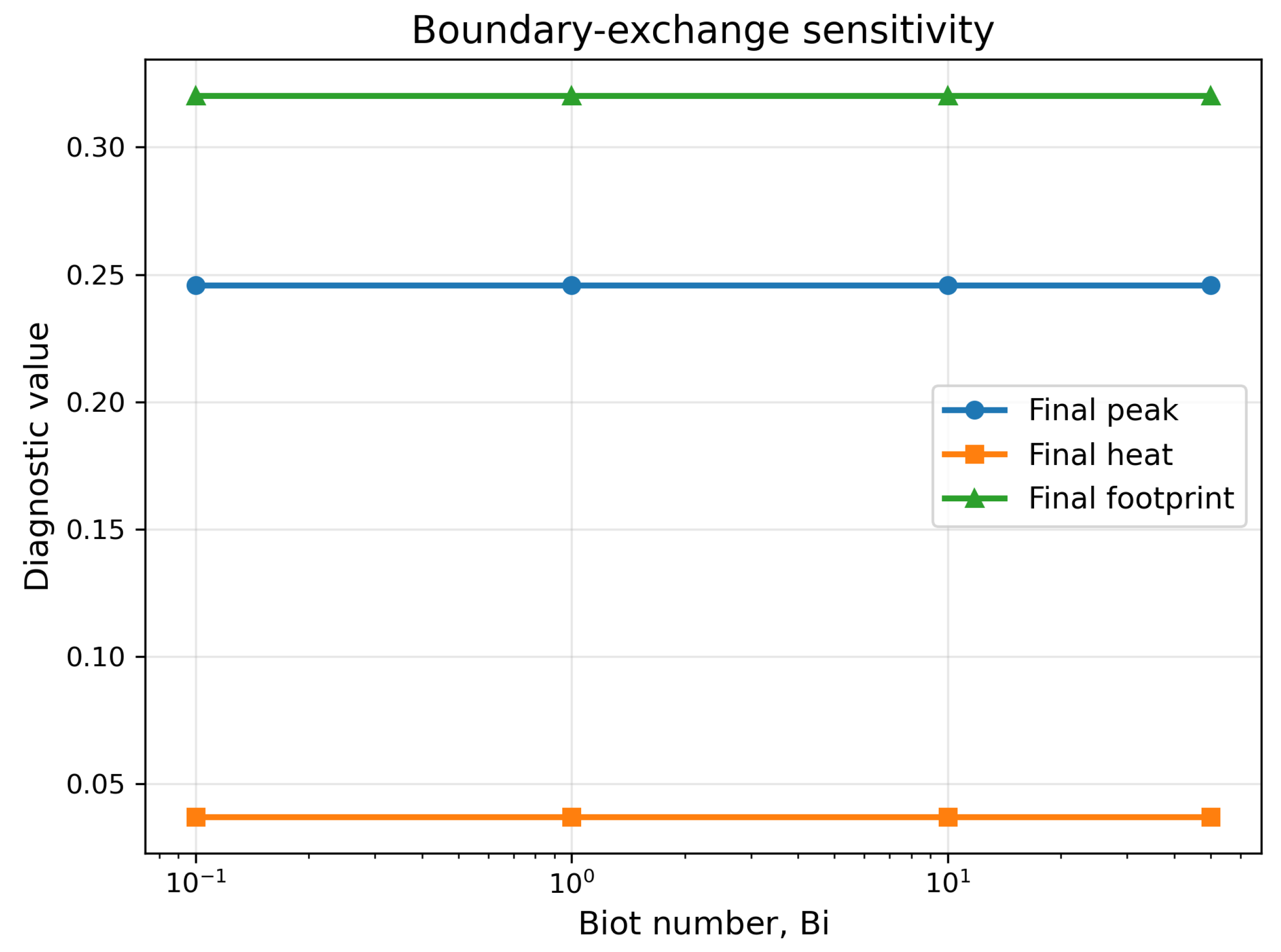
Boundary-exchange effect obtained by varying . The near-overlap of the diagnostic curves indicates that boundary exchange is weak relative to memory, nonlinear mobility, and heterogeneity over the present time window.
Figure 17.
Boundary-exchange effect obtained by varying . The near-overlap of the diagnostic curves indicates that boundary exchange is weak relative to memory, nonlinear mobility, and heterogeneity over the present time window.
Figure 18.
Final diagnostic values across . The final peak, heat content, and footprint remain unchanged to the displayed precision.
Figure 18.
Final diagnostic values across . The final peak, heat content, and footprint remain unchanged to the displayed precision.
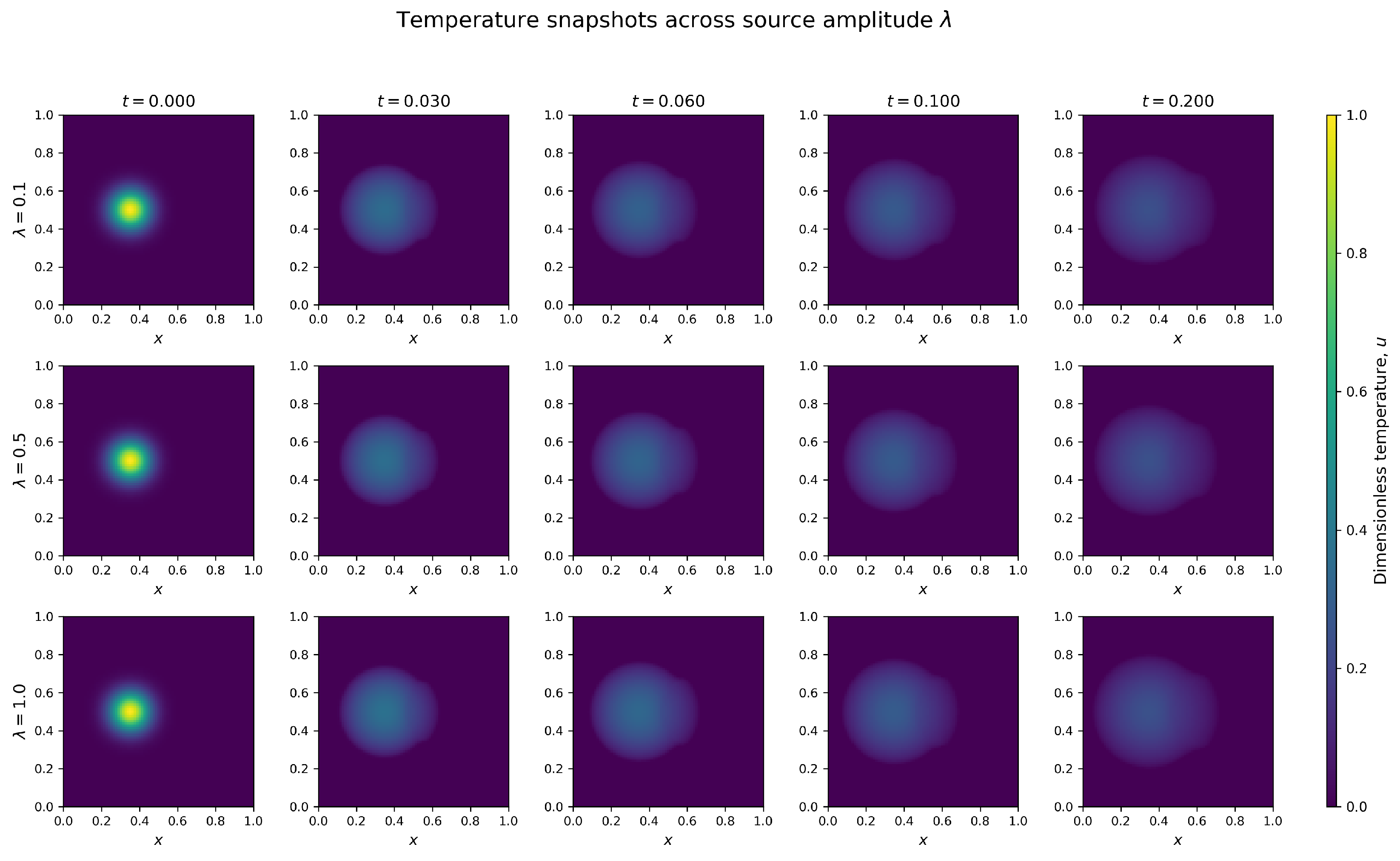
Figure 19.
Temperature snapshots across moderate source amplitudes at fixed , , and . Increasing raises the thermal response while preserving the underlying spatial organization.
Figure 19.
Temperature snapshots across moderate source amplitudes at fixed , , and . Increasing raises the thermal response while preserving the underlying spatial organization.
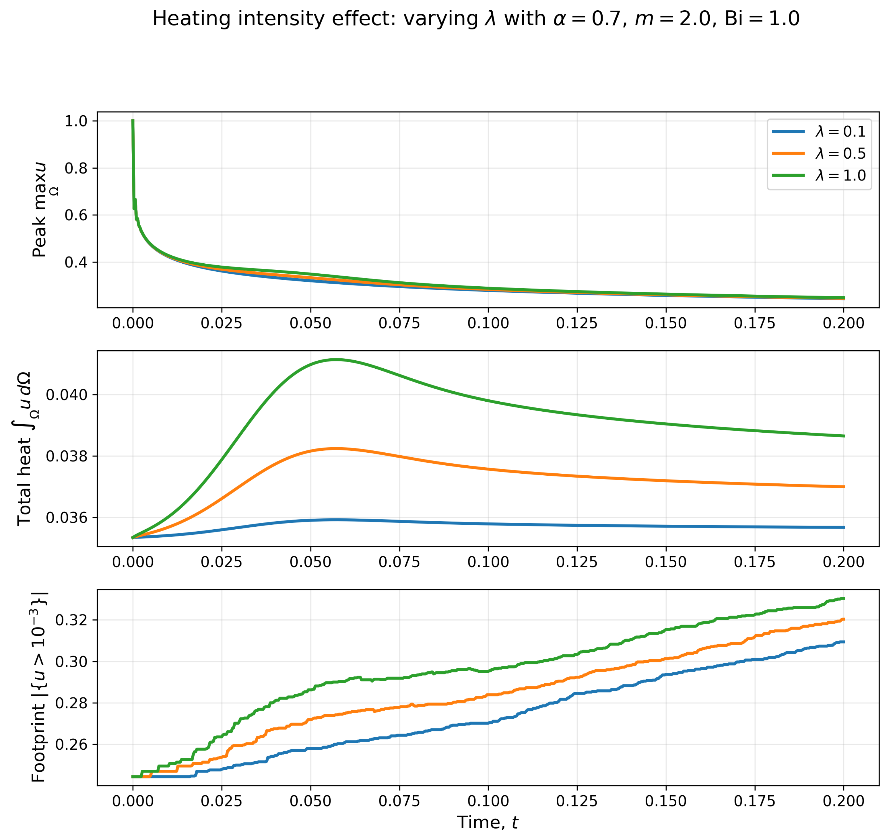
Figure 20.
Heating-intensity effect obtained by varying . Larger source amplitude increases heat content and footprint, but the transport pattern remains controlled by the memory, nonlinearity, and heterogeneity.
Figure 20.
Heating-intensity effect obtained by varying . Larger source amplitude increases heat content and footprint, but the transport pattern remains controlled by the memory, nonlinearity, and heterogeneity.
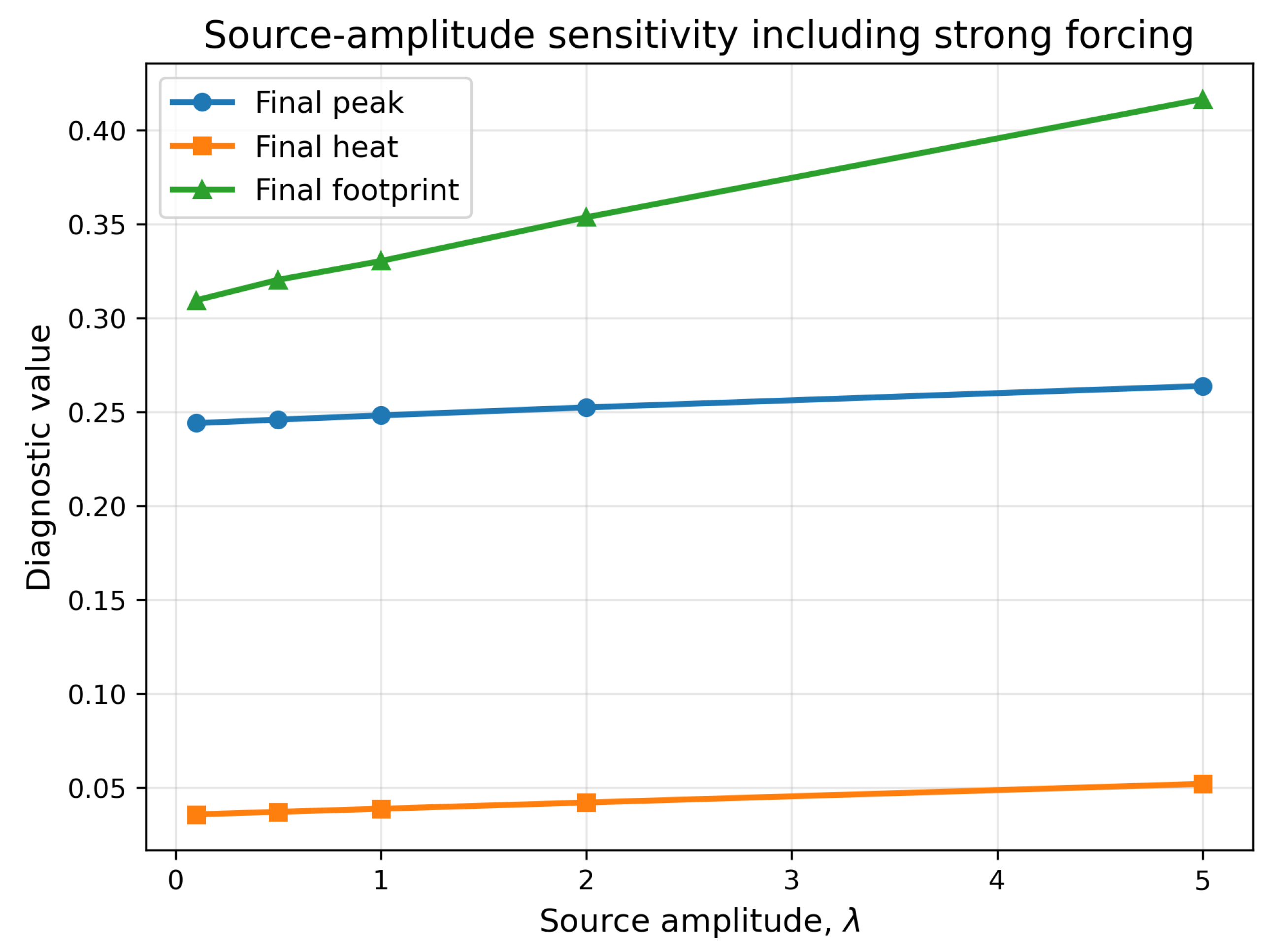
Figure 21.
Source-amplitude sensitivity including strong forcing. The final peak, heat content, and footprint increase monotonically with , but no abrupt localization-spreading transition is observed over the tested range.
Figure 21.
Source-amplitude sensitivity including strong forcing. The final peak, heat content, and footprint increase monotonically with , but no abrupt localization-spreading transition is observed over the tested range.
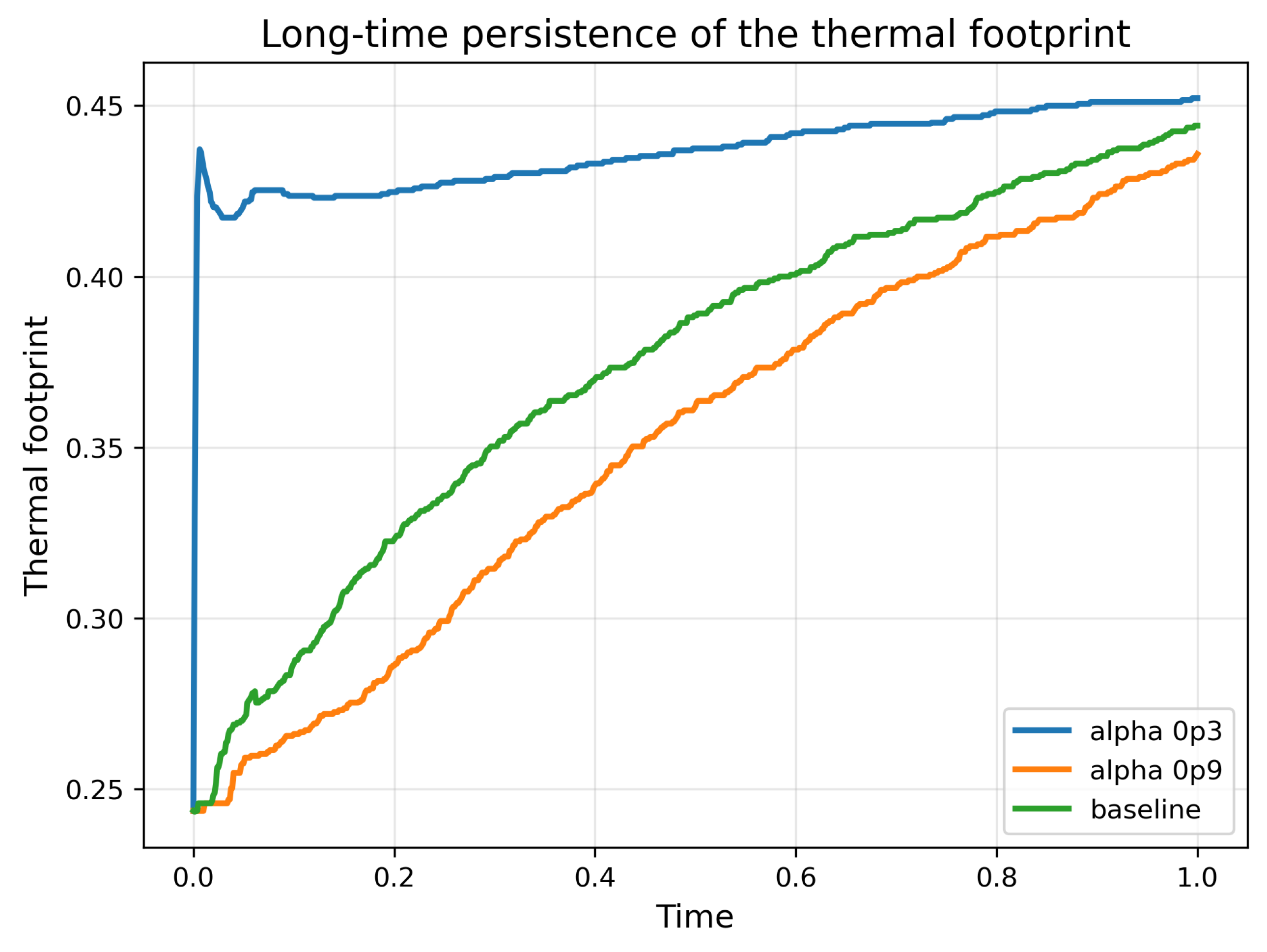
Figure 22.
Long-time persistence of the thermal footprint. The strong-memory case exhibits rapid early footprint expansion and remains spatially persistent over the longer interval, while the baseline and weak-memory cases evolve more gradually.
Figure 22.
Long-time persistence of the thermal footprint. The strong-memory case exhibits rapid early footprint expansion and remains spatially persistent over the longer interval, while the baseline and weak-memory cases evolve more gradually.
Table 1.
Model parameters, values used in the simulations, physical interpretation, and supporting references.
Table 1.
Model parameters, values used in the simulations, physical interpretation, and supporting references.
| Parameter | Value/Range Used | Physical Meaning | Reference or Justification |
|---|
| – | Strength of fractional thermal memory | [23,26,27] |
| m | – | Nonlinear porous-medium mobility exponent | [3,14] |
| 1–3 | Dimensionless conductivity heterogeneity | [22,23] |
| – | Dimensionless source-strength parameter | Sensitivity range based on nondimensional heating scale |
| Gaussian pulse | Localized volumetric thermal excitation | [22,24] |
| –50 | Boundary heat exchange strength | [22,28] and extended sensitivity testing |
| – | Numerical coefficient-level regularization | Sensitivity test for degeneracy control |
| Gaussian profile | Initial dimensionless temperature rise | [22] |
Table 2.
Manufactured-solution verification under coupled space-time refinement. The errors are measured at the final time.
Table 2.
Manufactured-solution verification under coupled space-time refinement. The errors are measured at the final time.
| | h | | | | Observed Rates |
|---|
| 40 | 160 | 0.025000 | 0.001250 | | | - |
| 60 | 240 | 0.016667 | 0.000833 | | | |
| 80 | 320 | 0.012500 | 0.000625 | | | |
| 100 | 400 | 0.010000 | 0.000500 | | | |
Table 3.
Computational cost and Picard iteration behavior under grid refinement for the reference physical configuration.
Table 3.
Computational cost and Picard iteration behavior under grid refinement for the reference physical configuration.
| | Problem Size | CPU Time (s) | Mean Picard | Max Picard | Final Peak | Final Footprint |
|---|
| 60 | 360 | 3721 | 475.38 | 32.625 | 50 | 0.246089 | 0.323056 |
| 70 | 420 | 5041 | 755.97 | 32.288 | 49 | 0.246499 | 0.322041 |
| 80 | 480 | 6561 | 1124.93 | 32.013 | 47 | 0.245855 | 0.320312 |
| 100 | 600 | 10201 | 4028.53 | 31.448 | 46 | 0.246225 | 0.316000 |
Table 4.
Sensitivity to conductivity structure. Percentage changes are computed relative to the circular heterogeneous baseline.
Table 4.
Sensitivity to conductivity structure. Percentage changes are computed relative to the circular heterogeneous baseline.
| Conductivity Structure | Final Peak | Final Heat | Final Footprint | Peak Change (%) | Heat Change (%) | Footprint Change (%) |
|---|
| Homogeneous | 0.251572 | 0.036998 | 0.295781 | | | |
| Circular heterogeneous | 0.245855 | 0.036998 | 0.320312 | | | |
| Smooth heterogeneous | 0.230904 | 0.036998 | 0.327500 | | | |
| Layered heterogeneous | 0.234257 | 0.036998 | 0.330156 | | | |
| Random smooth heterogeneous | 0.205790 | 0.037028 | 0.361406 | | | |
Table 5.
Sensitivity to fractional order . Percentage changes are computed relative to the baseline .
Table 5.
Sensitivity to fractional order . Percentage changes are computed relative to the baseline .
| Final Peak | Final Heat | Final Footprint | Peak Change (%) | Heat Change (%) | Footprint Change (%) |
|---|
| 0.3 | 0.237764 | 0.037052 | 0.411562 | | | |
| 0.5 | 0.244405 | 0.037182 | 0.362813 | | | |
| 0.7 | 0.245855 | 0.036998 | 0.320312 | | | |
| 0.9 | 0.239628 | 0.036741 | 0.282031 | | | |
Table 6.
Sensitivity to porous-medium exponent m. Percentage changes are computed relative to the baseline .
Table 6.
Sensitivity to porous-medium exponent m. Percentage changes are computed relative to the baseline .
| m | Final Peak | Final Heat | Final Footprint | Peak Change (%) | Heat Change (%) | Footprint Change (%) |
|---|
| 1.5 | 0.187862 | 0.036915 | 0.485938 | | | |
| 2.0 | 0.245855 | 0.036998 | 0.320312 | | | |
| 3.0 | 0.343923 | 0.036998 | 0.257656 | | | |
| 4.0 | 0.420434 | 0.036998 | 0.257656 | | | |
Table 7.
Sensitivity to boundary exchange. Percentage changes are computed relative to the baseline .
Table 7.
Sensitivity to boundary exchange. Percentage changes are computed relative to the baseline .
| Final Peak | Final Heat | Final Footprint | Peak Change (%) | Heat Change (%) | Footprint Change (%) |
|---|
| 0.1 | 0.245855 | 0.036998 | 0.320312 | | | |
| 1.0 | 0.245855 | 0.036998 | 0.320312 | | | |
| 10.0 | 0.245855 | 0.036998 | 0.320312 | | | |
| 50.0 | 0.245855 | 0.036998 | 0.320312 | | | |
Table 8.
Sensitivity to source amplitude, including strong forcing. Percentage changes are computed relative to the baseline .
Table 8.
Sensitivity to source amplitude, including strong forcing. Percentage changes are computed relative to the baseline .
| Final Peak | Final Heat | Final Footprint | Peak Change (%) | Heat Change (%) | Footprint Change (%) |
|---|
| 0.1 | 0.243992 | 0.035674 | 0.309375 | | | |
| 0.5 | 0.245855 | 0.036998 | 0.320312 | | | |
| 1.0 | 0.248105 | 0.038654 | 0.330313 | | | |
| 2.0 | 0.252373 | 0.041965 | 0.353594 | | | |
| 5.0 | 0.263748 | 0.051897 | 0.416563 | | | |
Table 9.
Sensitivity to coefficient-level regularization. Percentage changes are computed relative to the baseline .
Table 9.
Sensitivity to coefficient-level regularization. Percentage changes are computed relative to the baseline .
| Final Peak | Final Heat | Final Footprint | Peak Change (%) | Heat Change (%) | Footprint Change (%) |
|---|
| 0.245855 | 0.036998 | 0.320312 | | | |
| 0.245855 | 0.036998 | 0.320312 | | | |
| 0.245855 | 0.036998 | 0.320312 | | | |
Table 10.
Long-time comparison of selected fractional orders at . Percentage changes are computed relative to the long-time baseline .
Table 10.
Long-time comparison of selected fractional orders at . Percentage changes are computed relative to the long-time baseline .
| Case | Final Peak | Final Heat | Final Footprint | Peak Change (%) | Heat Change (%) | Footprint Change (%) |
|---|
| 0.177711 | 0.036305 | 0.444167 | | | |
| 0.208293 | 0.035965 | 0.452222 | | | |
| 0.152754 | 0.036501 | 0.435833 | | | |