Article

Approximate Analytical Solutions for a Nonlinear Model of Corneal Curvature Using the Homotopy Perturbation Method in Conjunction with the Least Squares Method


by
Olivia Bundău
and
Bogdan Căruntu
*,†
Department of Mathematics, Politehnica University of Timişoara, 300006 Timişoara, Romania
*
Author to whom correspondence should be addressed.
These authors contributed equally to this work.
Mathematics 2026, 14(12), 2185; https://doi.org/10.3390/math14122185
Submission received: 17 May 2026 / Revised: 9 June 2026 / Accepted: 15 June 2026 / Published: 17 June 2026

Abstract

In this paper we apply the Homotopy Perturbation Method in conjunction with the Least Squares Method to obtain, in a simple and straightforward manner, analytical approximations of the solutions for the nonlinear models of the corneal curvature. The partially linearized version of the model is extensively studied, and we included a comparison with previous results obtained by other well-known methods. On the other hand, for the fully nonlinear version of the model, we introduce for the first time an accurate analytical approximation of the solution.

1. Introduction

The eye is one of the most important and sensitive organs of the human body. The cornea, the crucial part of the eye that covers the iris, pupil, and anterior chamber, refracts light and accounts for approximately two-thirds of the eye’s total optical power. Many sight disorders (myopia, hyperopia, and astigmatism) can be traced to wrong corneal geometry. For this reason, precise knowledge of corneal topography is needed, especially since the success of medical diagnosis and interventions such as refractive surgery and the fitting of a contact lens depend strongly on this knowledge.
There are several types of mathematical models of the cornea currently in use, with various degrees of accuracy, such as models based on surfaces of revolution, mostly parabolas and ellipses [1]; models based on generalized conics with variable eccentricity [2]; shell theory based models [3]; models of corneal biomechanics based on the finite element method [4]; models based on Zernike polynomial approximations [5]; models based on Fourier series methods to describe the shape of crystalline lens [6]; and models consisting of fractional boundary value problems [7].
The model studied in the present paper is a nonlinear one, fitting optical data measurements of corneal shapes with high accuracy [8]. It consists of a two-point boundary value problem where two variants of the second-order ordinary differential equation included were proposed, a highly nonlinear one and partially linearized one. The existence and uniquity of the solutions is already established for both versions of the model [8,9].
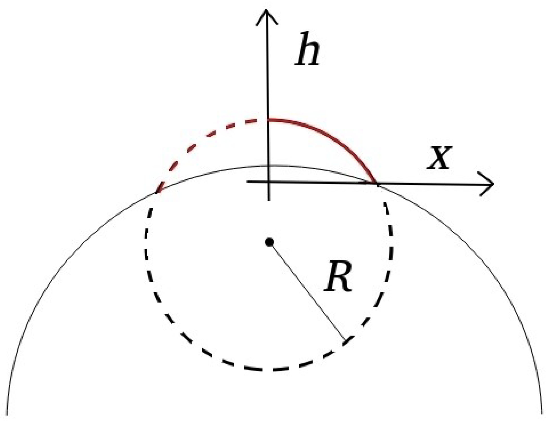
The mathematical model [8] assumes that the corneal geometry is axisymmetric with radius R (see Figure 1) and considers the section h = h ( x ) through the cornea (corneal surface height), where x is the distance from the center of symmetry (which is the origin of the system of coordinates). Thus the curve h ( x ) can be considered a meridian of a surface of revolution describing the corneal geometry.
In this model the function h is assumed to be a C2 function [8].
The equation is obtained by balancing the acting forces: the intraocular pressure acting in a normal direction to the cross-section of the cornea, the tension acting tangentially, and the spring force proportional to h.
The variables are rescaled to the non-dimensional form (but we retain the original notation for clarity), and we denote a = k · R 2 T and b = P · R T , where:
  • R is the radius of the corneal section
  • P is the intraocular pressure acting in a normal direction to the cross-section of cornea
  • T is the tension acting tangentially
  • k is the elastic constant of the spring force proportional to h (introduced to model the elastic features of the cornea)
Thus the fully nonlinear version of the model is [8]:
d 2 h d x 2 ( 1 + ( d h d x ) 2 ) 3 2 a · h + b ( 1 + ( d h d x ) 2 ) 1 2 = 0 , x [ 0 , 1 ] h ( 1 ) = 0 , d h d x ( 0 ) = 0
If one assumes that the deflection of the corneal surface is small, then the partially linearized version of the model is obtained [8]:
d 2 h d x 2 a · h + b ( 1 + ( d h d x ) 2 ) 1 2 = 0 , x [ 0 , 1 ] h ( 1 ) = 0 , d h d x ( 0 ) = 0
For the partially linearized model (2) several well-known methods were employed to find approximations of the solution, such as the zero-order solution based on the hyperbolic cosine function [8], Taylor series based methods [10], the Homotopy Perturbation Method [11], the perturbation method [12], the linearization approach [12], the Green’s function method [13] or the residual power series method [14].
For the full nonlinear version of the model (1) some numerical approximation methods were proposed, such as the method of lines for the partial differential equation associated with the model [15], but, to the best of our knowledge, no accurate analytical approximate solution was proposed so far. We will introduce such an approximation in Section 4.
In order to compute approximations for the problems (1)/(2), we will employ the Homotopy Perturbation Method in conjunction with the Least Squares Method, denoted in the following by HPMLS.
HPMLS was introduced relatively recently [16,17,18], and it is based on the well-known Homotopy Perturbation Method [19,20]. The Homotopy Perturbation Method (HPM) is by itself capable of providing accurate approximation for many types of problems. HPMLS, by combining HPM and the Least Squares Method, is able to provide even more accurate approximations but also retains the straightforward manner of computing solutions characteristic of HPM.
The main features of HPMLS are:
  • Accelerated convergence compared to the regular HPM and most other similar methods.
  • Very accurate approximate analytical solutions.
  • Possible application for problems defined on wide (even infinite) intervals for the variables.
  • Possible application to a wide range of nonlinear problems (ODEs, PDEs, integro-differential equations, optimal problems, etc.).

2. Homotopy Perturbation Method in Conjunction with the Least Squares Method (HPMLS)

The Homotopy Perturbation Method (HPM) was introduced by J.H.He [19,20] and is one of the most well-known and powerful methods for obtaining approximate analytical solutions for nonlinear problems.
We consider the general problem:
A ( h ( x ) ) f ( x ) = 0 , B ( h ) = 0
where A is a general differential operator, f ( x ) is a known analytical function [19] and B represents the boundary conditions.
f ( x ) is also sometimes called a “source term” and may be an analytical forcing function or non-homogeneous term dictated directly by the original governing differential problem (3).
We mention that in the case of the problems (1)/(2) the function f ( x ) is actually chosen as f ( x ) = 0 , so in the following we will omit it.
In order to find approximations for a problem of the type (3), the initial problem (3) is rewritten as [19]:
L ( h ( x ) ) + N ( h ( x ) ) = 0 , B ( h ) = 0
where:
  • L is a linear differential operator, chosen in such a way that the problem L ( h ( x ) ) = 0 is easily solvable and, if possible, characterizes the dominant behavior of the system.
  • N is a nonlinear operator that represents the rest of the problem (such that L + N = A ).
We remark the fact that while there are some guidelines regarding the choice of the operators L and N for certain type of problems [21], there are no universal rules in this regard; for the problems (1)/(2) we tested several of these possible choices.
If we denote by h ˜ an approximate solution of (4), we can evaluate the error obtained by replacing the exact solution h with the approximation h ˜ as the remainder:
R ( x , h ˜ ) = L ( h ˜ ( x ) ) + N ( h ˜ ( x ) ) , x R
The next step in applying HPMLS is to attach to (4) the following family of equations [19,20]:
( 1 p ) [ L ( Φ ( x , p ) ) ] + p [ L ( Φ ( x , p ) ) + N ( Φ ( x , p ) ) ] = 0
where p [ 0 , 1 ] is the embedding parameter and Φ ( x , p ) , called the homotopy solution, is a function satisfying the same properties as the solution of the initial problems (1)/(2), i.e., is of class C 2 .
The main property of Φ ( x , p ) is the fact that, on the one hand, when the embedding parameter has the value p = 0 , it becomes Φ ( x , 0 ) = h 0 ( x ) , where h 0 ( x ) is the solution of the following linear problem (a solution that can be readily found):
L ( h 0 ( x ) ) = 0 , B ( h 0 ) = 0
and, on the other hand, when the embedding parameter has the value p = 1 , it becomes Φ ( x , 1 ) = h ( x ) , which is in fact the solution of the initial nonlinear problem (4).
Thus, as p increases from 0 to 1, the homotopy solution Φ ( x , p ) varies from h 0 ( x ) to the solution h ( x ) of the initial problem.
Next we consider the following power series expansion of the homotopy solution Φ ( x , p ) :
Φ ( x , p ) = h 0 ( x ) + n 1 h n ( x ) p n
By substituting the expression (8) in (6), by collecting the same powers of p and by equating each coefficient of the powers of p with zero, we obtain:
L ( h n ( x ) ) = N n 1 ( h 0 ( x ) , h 1 ( x ) , , h n 1 ( x ) ) n 1 , , B ( h n ) = 0 ,
where N i , i 0 are the coefficients of p i in the nonlinear operator N :
N ( h ( x ) ) = N 0 ( h 0 ( x ) ) + p N 1 ( h 0 ( x ) , h 1 ( x ) ) + p 2 N 2 ( h 0 ( x ) , h 1 ( x ) , h 2 ( x ) ) +
In other words we obtained a recursive set of solvable linear Equation (9) by grouping and solving equations for each identical power of the embedding parameter p, and the solutions h n , n 1 are obtained from the linear Equation (9), which are easily solved together with the boundary conditions.
In theory, once h n , n 1 are computed, the solution of the initial problem can be found by taking the limit as p 1 in (8):
h ( x ) = lim p 1 Φ ( x , p ) = lim p 1 h 0 ( x ) + n 1 h n ( x ) p n = h 0 ( x ) + n 1 h n ( x )
However, in practice, due mostly to computational limitations, only solutions up to order m are actually computed, i.e., h 0 , h 1 , , h m , as solutions of the linear problems (7) and (9).
Thus the approximative solution of order m provided by the regular Homotopy Perturbation Method is the function f m ( x ) where:
h ( x ) h 0 ( x ) + n 1 m h n ( x ) = h 0 ( x ) + h 1 ( x ) + + h m ( x ) f m ( x )
We consider the set S m ( m = 0 , 1 , 2 , ) containing the functions φ m 0 , φ m 1 , φ m 2 , , φ m n , chosen as linearly independent functions in the vector space of the continuous functions on the real interval I such that S m 1 S m and h 0 + h 1 + + h m is a real linear combination of these functions.
We note that such a construction is always possible. For example we can choose S m = { h 0 , h 1 , , h m } , m = 0 , 1 , 2 , . In this case φ m 0 = x 0 , φ m 1 = h 1 , φ m 2 = h 2 , , φ m n = h m .
Definition 1 
([16]). We call an HP-sequence of problem (4) a sequence of functions { s m ( x ) } m N of the form s m ( x ) = k = 0 n m α m k φ m k , where m N , α m k R .
A function of the sequence is called an HP-function of problem (4).
We call the HP-sequence { s m ( x ) } m N convergent to the solution of problem (4) if lim m R ( x , s m ( x ) ) = 0 .
Definition 2 
([16]). We call an ϵ-approximate HP-solution of problem (4) on the real interval I an HP-function h ˜ , which satisfies the following condition:
| R ( x , h ˜ ) | < ϵ
together with the boundary conditions from (4).
Definition 3 
([16]). We call a weak δ-approximate HP-solution of problem (4) on the real interval I a HP-function h ˜ satisfying the relation I R 2 ( x , h ˜ ) dx δ , together with the boundary conditions from (4).
Remark 1. 
The ϵ-approximate HP-solution is the “natural” way of introducing an approximation, namely, as the approximation which, when replaced in the equation, yields a remainder (5) whose error is smaller than a given (desired) ϵ; however due to the way the Least Squares Method works, the approximations computed by using this method are in fact weak δ-approximate HP-solutions (see also Remark 2 at the end of this section).
In the next phase of applying HPMLS, we will find a weak ϵ -approximate HP-solution of the type:
h ˜ = k = 0 n m c m k φ m k
where m 0 and the constants c m k are computed using the following steps:
  • By imposing the boundary conditions, we can determine l N , l m such that c 0 m , c 1 m , , c l m are computed as functions of c l + 1 m , c l + 2 m , , c n m .
  • We substitute the approximate solution h ˜ in the initial equation and obtain the expression:
    R ( x , c m k ) = R ( x , h ˜ )
  • We attach to the problem the following real functional:
    J ( c m k ) = I R 2 ( x , c m k ) dt
  • We compute the values of c ˜ l + 1 m , c ˜ l + 2 m , , c ˜ n m as the values that give the minimum of the functional (14) and the values of c ˜ 0 m , c ˜ 1 m , , c ˜ l m again as functions of c ˜ l + 1 m , c ˜ l + 2 m , , c ˜ n m by using the boundary conditions.
  • Using the constants c ˜ 0 m , , c ˜ n m thus determined, we consider the HP-sequence:
    s m ( x ) = k = 0 n m c ˜ m k φ m k
The following convergence theorem holds:
Theorem 1 
([16]). The HP-sequence s m ( x ) from (17) satisfies the property:
lim m I R 2 ( x , s m ( x ) ) dx = 0
Moreover, ϵ > 0 , m 0 N such that m N , m > m 0 ; it follows that s m ( x ) is a weak ϵ-approximate HP-solution of problem (4).
Proof. 
Based on the way the HP-function s m ( x ) is computed, the following inequality holds:
0 I R 2 ( x , s m ( x ) ) dx I R 2 ( x , f m ( x ) ) dx , m N .
It follows that:
0 lim m I R 2 ( x , s m ( x ) ) dx lim m I R 2 ( x , f m ( x ) ) dx = 0 , m N .
We obtain:
lim m I R 2 ( x , s m ( x ) ) dx = 0 .
From this limit we obtain that ϵ > 0 , m 0 N such that m N , m > m 0 ; it follows that s m ( x ) is a weak ϵ -approximate HP-solution of problem (4) q.e.d. □
Remark 2 
([16]). Any ϵ-approximate HP-solution of problem (4) is also a weak approximate HP-solution, but the opposite is not always true. It follows that the set of weak approximate HP-solutions of problem (4) also contains the approximate HP-solutions of the problem.
Taking into account the above remark, in order to find ϵ -approximate HP-solutions of problem (4) by the HPMLS method we will first determine weak approximate HP-solutions, h ˜ . If | R ( x , h ˜ ) | < ϵ then h ˜ is also an ϵ -approximate HP-solution of the problem.

3. Numerical Results for the Partially Linearized Model

In this section we apply HPMLS for the case of the partially linearized model (2) and compare our approximate solutions to previously computed ones by means of other methods. In the computations we assumed for the parameters the values a = b = 1 for the sake of the comparison, since these were the values used most often in previous studies of the model. However, we remark the fact that for other values of the parameters in the permitted range [8], the results of the comparison are basically the same.
It is well known that for a given problem there is more than one possible choice of the homotopy (4), and, while there are some guidelines regarding this choice, there is no definitive rule in choosing the best homotopy, i.e., the one leading the the greater accuracy of the approximation. We considered several of the variants available and in the following we present the two ones that are not only the most straightforward ones but are also the ones leading to the best results.

3.1. Homotopy No. 1

The simplest choice of homotopy for (2) is:
L ( h ( x ) ) = d 2 h d x 2 , N ( h ( x ) ) = a · h + b ( 1 + ( d h d x ) 2 ) 1 2 , f ( x ) = 0
For this choice of homotopy, the approximations by the regular Homotopy Perturbation Method are (12):
f 0 = 0 f 1 = t 2 2 1 2 f 2 = t 4 24 + t 2 4 5 24 f 3 = t 6 720 + t 4 48 17 t 2 48 + 241 720 ;
It follows that the corresponding sets S m = { φ m 0 , φ m 1 , φ m 2 , , φ m n } are:
S 1 = { 1 , t 2 } S 2 = { 1 , t 2 , t 4 } S 3 = { 1 , t 2 , t 4 , t 6 }
Thus, for example, the first-order HPMLS approximation is computed starting with the function (14):
h ˜ = c 0 · 1 + c 1 · t 2
The corresponding boundary conditions are h ˜ ( 1 ) = 0 , d h ˜ d x ( 0 ) = 0 . The second condition is satisfied for any values of the constants, but from the first one we obtain c 0 = c 1 and the function becomes:
h ˜ = c 1 + c 1 · t 2
The corresponding remainder (5) and (15) is:
R ( x , c 1 ) = c 1 · t 2 + 3 · c 1 + 1 4 · c 1 2 · t 2 + 1
The attached functional (16) is:
J ( c 1 ) = 0 1 c 1 2 · t 4 6 · c 1 2 · t 2 + 9 · c 1 2 + 1 4 · c 1 2 · t 2 + 1 + 6 · c 1 4 · c 1 2 · t 2 + 1 2 · c 1 · t 2 4 · c 1 2 · t 2 + 1 dt
It is possible to compute the integral directly, but the very complicated expression of the result leads in turn to a poor result of the following minimization step. As a consequence, we computed an approximation of the integral based on an iterative Simpson’s formula. The value of the constant c 1 , which minimizes the functional (24), is c 1 = 0.3493695429331202 , and applying again the boundary condition ( c 0 = c 1 ) we obtain the first-order HPMLS approximation:
h ˜ 1 = 0.3493695429331202 · t 2 + 0.3493695429331202
In a similar manner we computed HPMLS approximations of increasing orders, some of which are presented below:
h ˜ 2 = 0.012659402577507197 · t 4 0.32780412949676757 · t 2 + 0.34046353207427477 h ˜ 3 = 0.00138413735430643 · t 6 0.0097048634130182 · t 4 0.32957045995305734 · t 2 + 0.34065946072038206 h ˜ 7 = 3.48722144378465534 · 10 6 · t 14 + 0.000022268822449 · t 12 0.000084865605770 · t 10 + 0.0002803103068016 · t 8 0.00185139400913 · t 6 0.00935884101508 · t 4 0.3296679970926 · t 2 + 0.34066400581479
In order to estimate the errors associated with these approximations, since of course there is no known exact solution of the problem, we used a numerical solution based on a Runge–Kutta method. Thus, the absolute errors of the approximations mentioned in the following (both ours and previously computed ones) are in fact the differences in absolute value between the approximation and the numerical solution given by the Runge–Kutta method. The relative errors are computed by dividing the absolute errors by the value of the numerical solution and multiplying by 100.
The following two tables present the absolute errors corresponding to the approximations presented above, computed by the regular HPM (19) (Table 1) and by HPMLS (26) (Table 2).
We remark that the data from the tables not only emphasize the accuracy of the HPMLS approximations, which are way more precise than their HPM counterparts, but also clearly illustrate the convergence of the method.

3.2. Homotopy No. 2

The other obvious choice of homotopy for (2) is:
L ( h ( x ) ) = d 2 h d x 2 a · h , N ( h ( x ) ) = b ( 1 + ( d h d x ) 2 ) 1 2 , f ( x ) = 0
For this choice of homotopy, the approximations by the regular Homotopy Perturbation Method are (12) (the expressions for the approximations of higher order are too long to include here):
f 0 = 0 f 1 = f 2 = 1 2 e cosh ( t ) 1 + e 2 f 3 = f 4 = 1 + e 2 e 2 cosh ( 2 t ) + 3 e 4 + 9 e 2 + 3 e 7 + 18 e 2 + 7 e 4 cosh ( t ) 3 1 + e 2 3
Then the corresponding sets S m = { φ m 0 , φ m 1 , φ m 2 , , φ m n } are:
S 1 , 2 = { 1 , cosh ( t ) } S 3 , 4 = { 1 , cosh ( t ) , cosh ( 2 · t ) } S 5 , 6 = { 1 , cosh ( t ) , cosh ( 2 · t ) , cosh ( 3 · t ) , cosh ( 4 · t ) , t · sinh ( t ) } S 7 , 8 = { 1 , cosh ( t ) , cosh ( 2 · t ) , cosh ( 3 · t ) , cosh ( 4 · t ) , cosh ( 5 · t ) , cosh ( 6 · t ) , t · sinh ( t ) , t · sinh ( 2 · t ) }
Using the same steps as before, we computed HPMLS approximations:
h ˜ 1 = 0.933565820546562 0.605001319751732 · cosh ( t ) h ˜ 3 = 1.06148742989955 0.744637239001054 · cosh ( t ) + 0.0232704199233330 cosh ( 2 · t ) h ˜ 5 = 2.57458961725276 2.03127072573423 · cosh ( t ) 0.216943543839818 · cosh ( 2 · t ) + 0.0149236983038703 · cosh ( 3 · t ) 0.000635051964305239 · cosh ( 4 · t ) + 1.05778004048562 · t · sinh ( t ) h ˜ 7 = 2.88920437406131 3.85127541021090 · cosh ( t ) + 1.03657070378163 · cosh ( 2 · t ) + 0.292027541410735 · cosh ( 3 · t ) 0.0279351011879268 · cosh ( 4 · t ) + 0.00215755706772406 · cosh ( 5 · t ) 0.0000856675737311516 · cosh ( 6 · t ) + 0.433907068187038 · t · sinh ( t ) 1.01357467291942 · t · sinh ( 2 · t )
The following table (Table 3) presents the absolute errors corresponding to both the approximations computed by the regular HPM ( f 3 , f 5 , f 7 ) and by HPMLS ( h ˜ 3 , h ˜ 6 , h ˜ 7 ).

3.3. Comparison with Previous Results

In the following we present a comparison between the approximations computed by HPMLS and previously computed approximations by other methods. Most of the data included here comes from paper [13], where the authors compared their own results with previous ones.
Included in this comparison are:
  • The seventh-order approximations computed by HPMLS in the previous sections by means of the two homotopies. Thus h ˜ 7 H 1 denotes the polynomial approximation obtained by means of the first homotopy, while h ˜ 7 H 2 denotes the approximation consisting of hyperbolic functions obtained by means of the second homotopy.
  • Approximation based on the hyperbolic cosine function [8] (via [13]), denoted by h h c s .
  • Taylor series based approximation [10] (via [13]), denoted by h t a y .
  • Approximation obtained by a linearization approach [12] (via [13]), denoted by h l i n .
  • Approximation obtained by the perturbation method [12] (via [13]), denoted by h p e r .
  • Green’s function method based approximation [13], denoted by h g r e .
  • Approximation by the residual power series method [14], denoted by h r e s .
Table 4 presents the relative errors corresponding to these approximations.
In order to further emphasize the accuracy of the approximations provided by HPMLS, Table 5 presents the percentage improvement achieved by h ˜ 7 H 1 over the previous approximations included in the comparison.
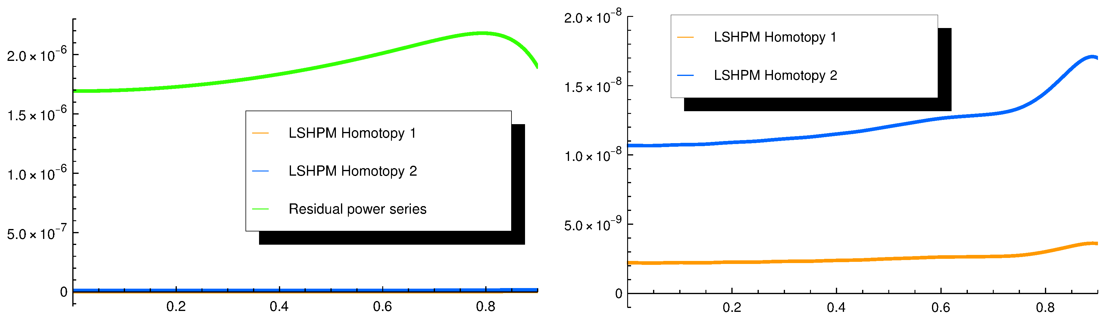
Figure 1 presents a comparison between our approximations and the most accurate previous one, computed by the residual power series method [14], whose expression is in fact of the same type as the one obtained by using our first homotopy, namely, a 14th-degree polynomial including even powers only. The figure presents the absolute errors corresponding to each approximation.
Regarding the practical significance of the observed error reductions illustrated by the previous tables and figures, we remark that while high precision may be considered unnecessary for the given problem of the approximation of the corneal shape, any subsequent computations involving such approximations (such as the discussion included in Section 4.2) can greatly benefit from an approximation that is both very precise and at the same type has a very simple expression. Indeed this is exactly the case for the approximations h ˜ i presented above.

4. Numerical Results for the Fully Nonlinear Model

4.1. HPMLS Approximations

In this section we apply HPMLS for the case of the fully nonlinear model (1), rewritten as:
d 2 h d x 2 a · h · ( 1 + ( d h d x ) 2 ) 3 2 + b · ( 1 + ( d h d x ) 2 ) = 0 , x [ 0 , 1 ] h ( 1 ) = 0 , d h d x ( 0 ) = 0
While some paper discuss this model [9,15], to the best of our knowledge no accurate approximations were proposed for this model.
For (31) we also considered several possible homotopies but, just as in the case of the partially linearized model, the best results were obtained by using the simplest one:
L ( h ( x ) ) = d 2 h d x 2 , N ( h ( x ) ) = a · h · ( 1 + ( d h d x ) 2 ) 3 2 + b · ( 1 + ( d h d x ) 2 ) , f ( x ) = 0
For this choice of homotopy, the corresponding sets S m = { φ m 0 , φ m 1 , φ m 2 , , φ m n } are again:
S 1 = { 1 , t 2 } S 2 = { 1 , t 2 , t 4 } S 3 = { 1 , t 2 , t 4 , t 6 }
Applying HPMLS we computed the approximations:
h ˜ 3 = 0.0302016813878762 · t 6 0.0175371331839689 · t 4 0.322742689412420 · t 2 + 0.370481503984265 h ˜ 4 = 0.0131661881939382 · t 8 + 0.00467522481404659 · t 6 0.0484100325974576 · t 4 0.313496101518893 · t 2 + 0.370397097496242 h ˜ 5 = 0.00550565599330535 · t 10 + 0.00424826731352766 · t 8 0.0148401812597214 · t 6 0.0394322888565011 · t 4 0.314937849236037 · t 2 + 0.370467708032037 h ˜ 6 = 0.00224529720417140 · t 12 + 0.00209349029670953 · t 10 0.00537615886426085 · t 8 0.00916276166645391 · t 6 0.0410198243797952 · t 4 0.314757579994286 · t 2 + 0.370468131812258 h ˜ 7 = 0.000885465695016480 · t 14 + 0.000804893538945844 · t 12 0.00191299291529202 · t 10 0.00284456667534224 · t 8 0.00996101333998758 · t 6 0.0409021604470165 · t 4 0.314766231488764 · t 2 + 0.370467537022473
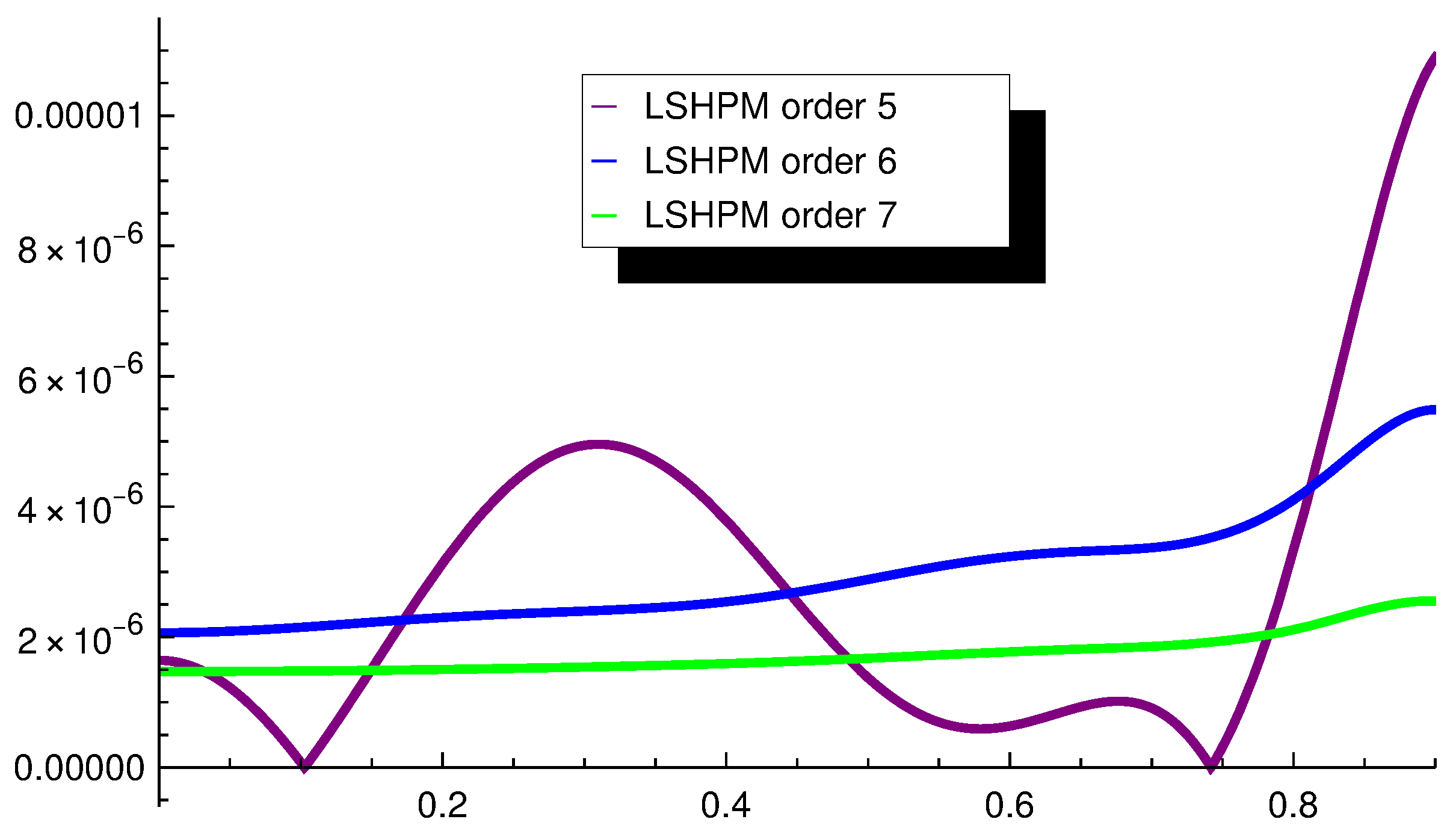
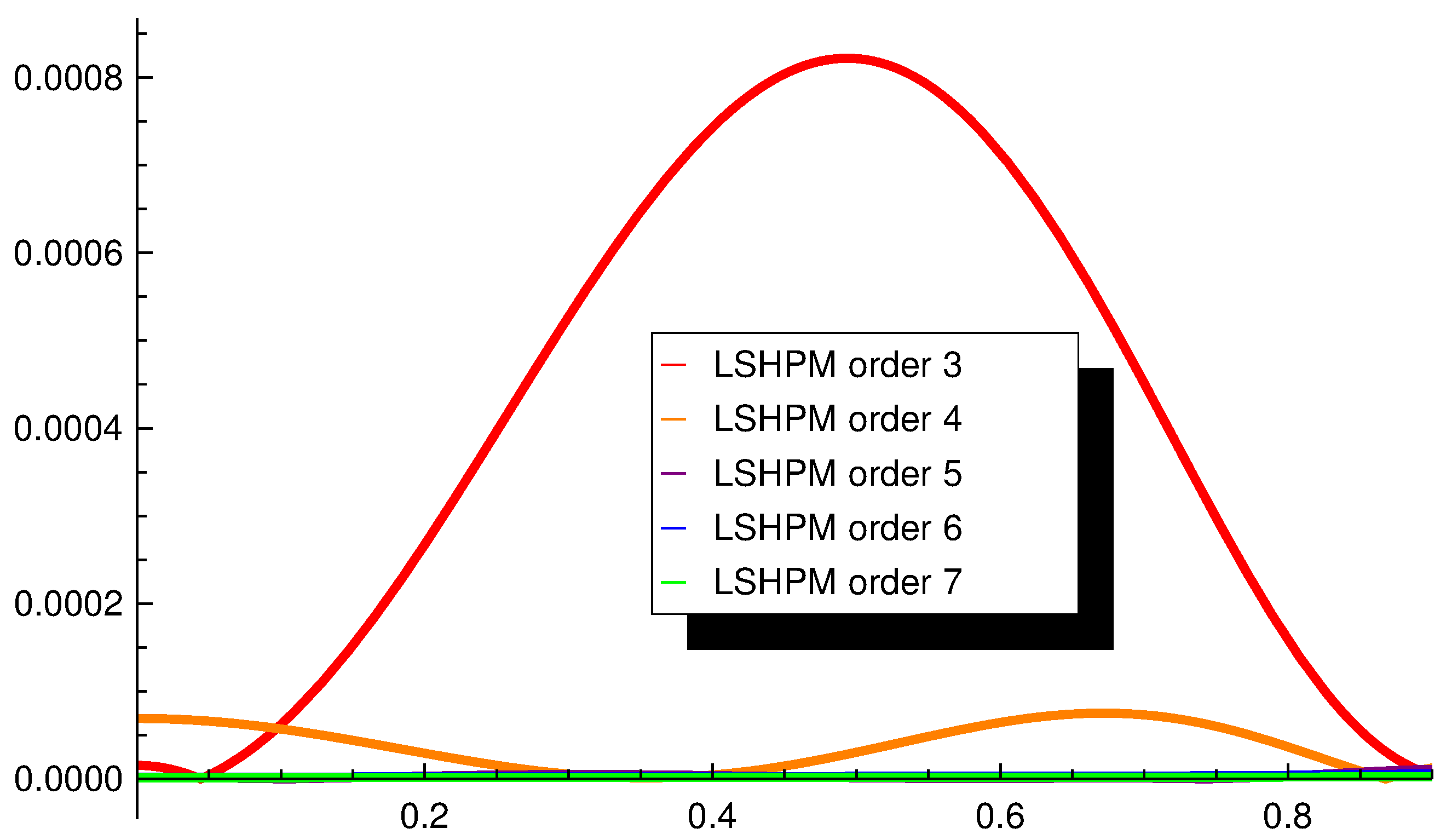
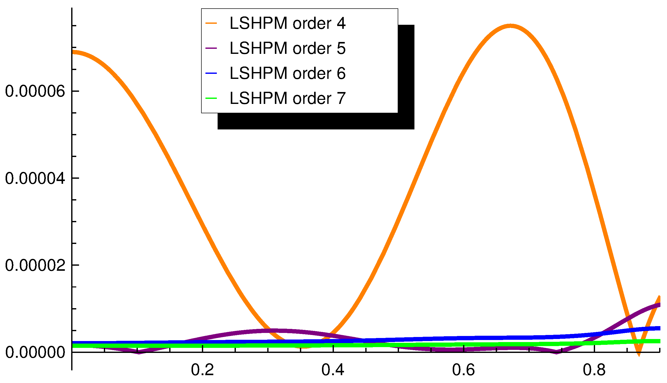
Table 6 and Figure 2, Figure 3, Figure 4 and Figure 5 present the relative errors corresponding to these approximations. As expected, since the nonlinearity of this model is much stronger, the errors are higher than the corresponding ones for the case of the linearized model, but overall they are still very low.

4.2. Discussion

In the following we include a brief qualitative study of the influence of the parameters a and b on the corneal shape h ( x ) as described by the model (31).
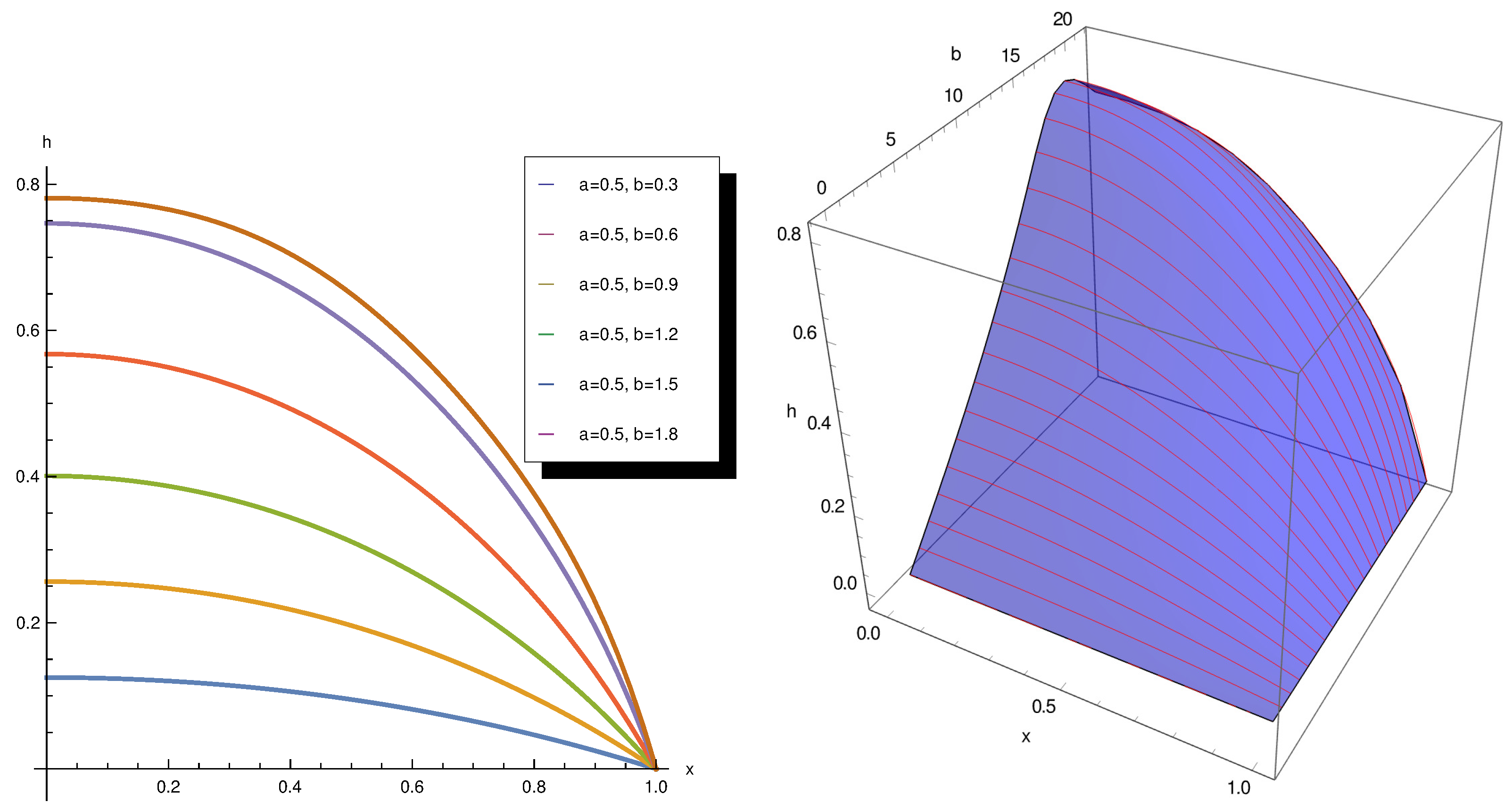
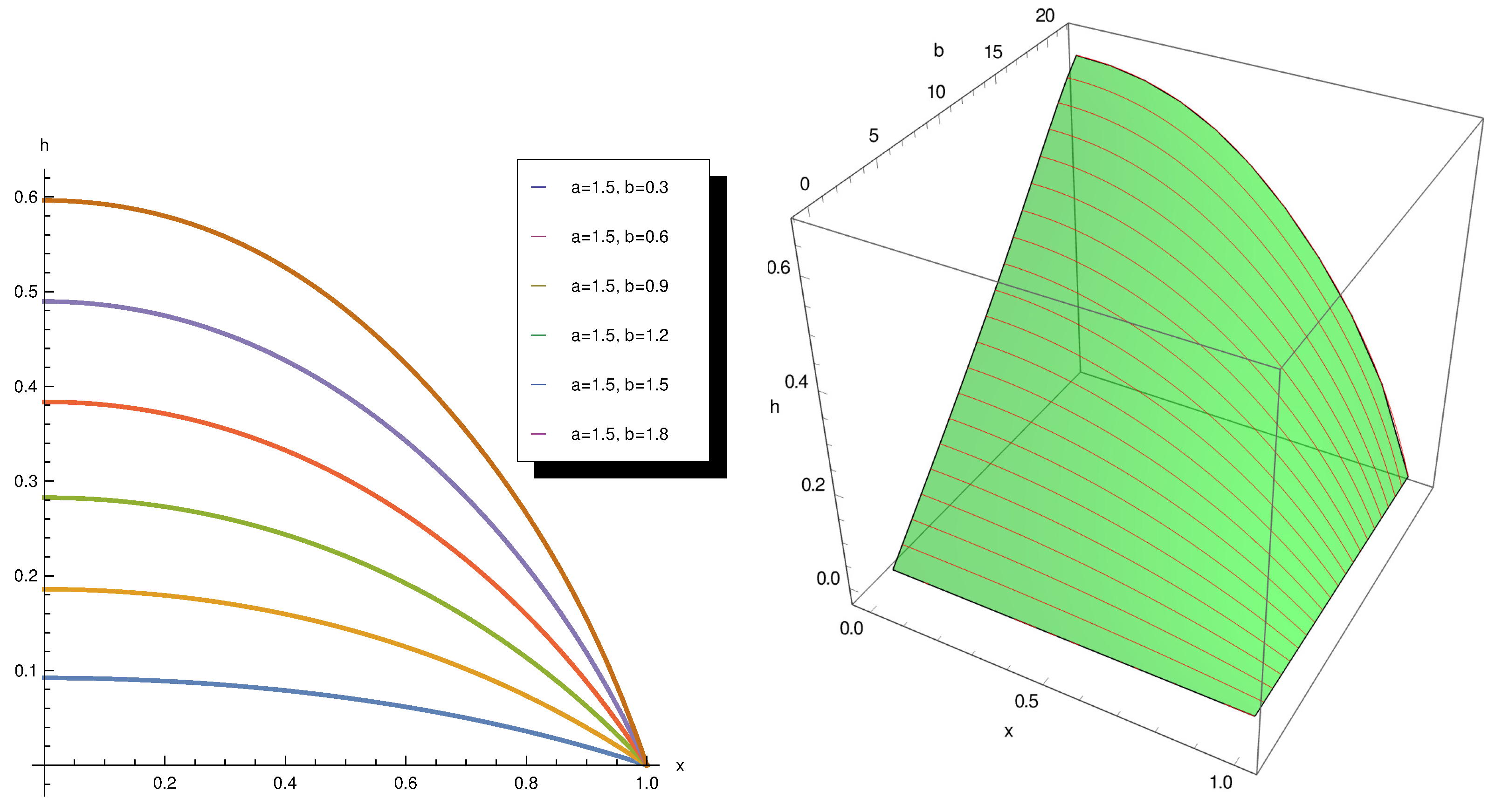
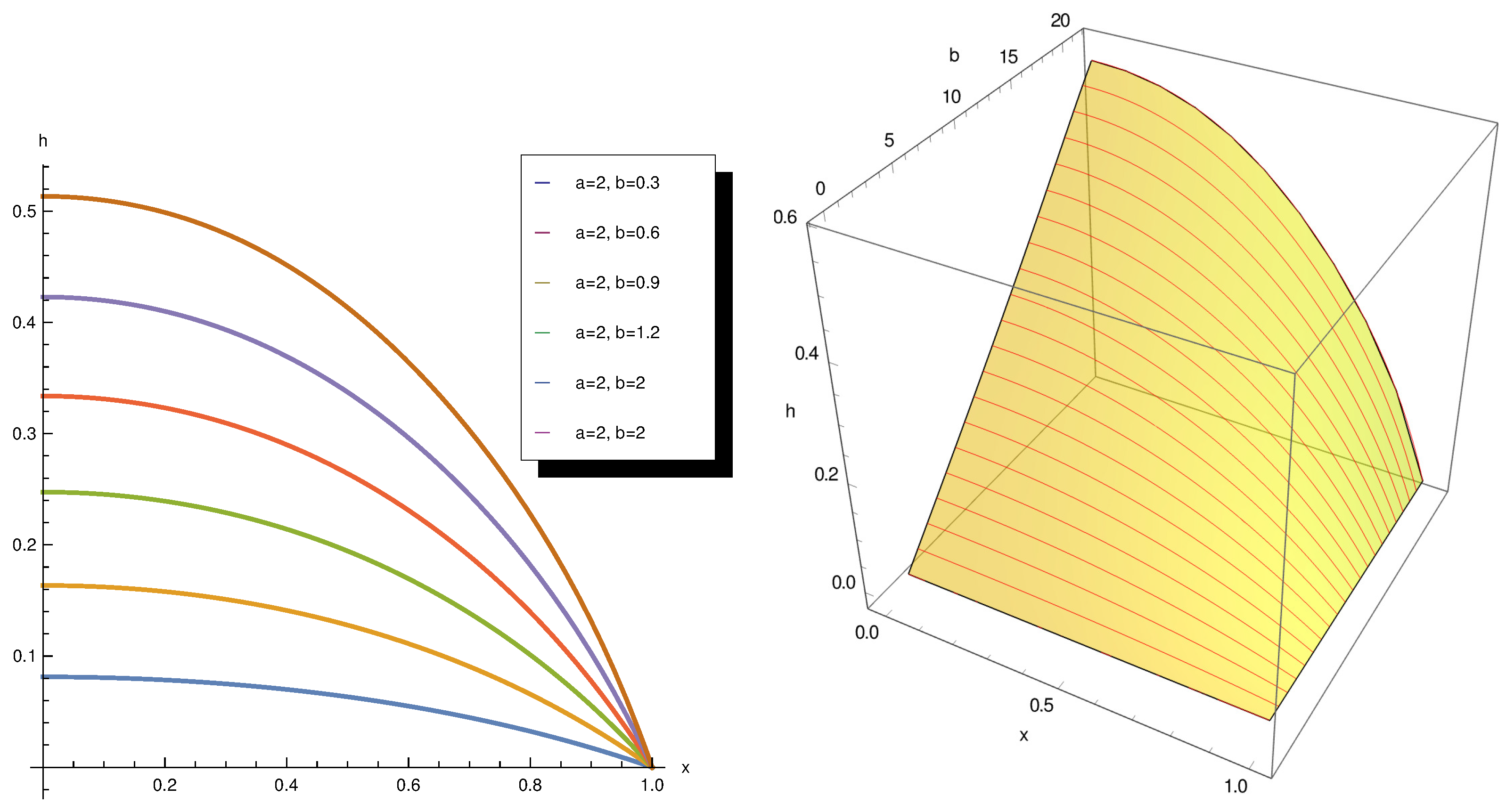
The parameters a and b are dimensionless constants, which in the model (1)/(2) represent the biomechanical and geometric state of the human cornea. As mentioned in the introduction, a = k · R 2 T and b = P · R T , where R is the corneal radius, P is the intraocular pressure, T is the tangential tension and k is the elastic constant. Thus a can be considered to represent the ratio of corneal curvature stiffness to its tension while b may be considered to represent the effect of the intraocular pressure relative to the cornea’s tension, and, together, a and b can be used to represent in a very precise way the radially symmetric sag or elevation of the cornea. Since the model is nonlinear, it can veridically simulate details such as the flattening of the cornea toward the periphery (which can be visualized in the last two figures).
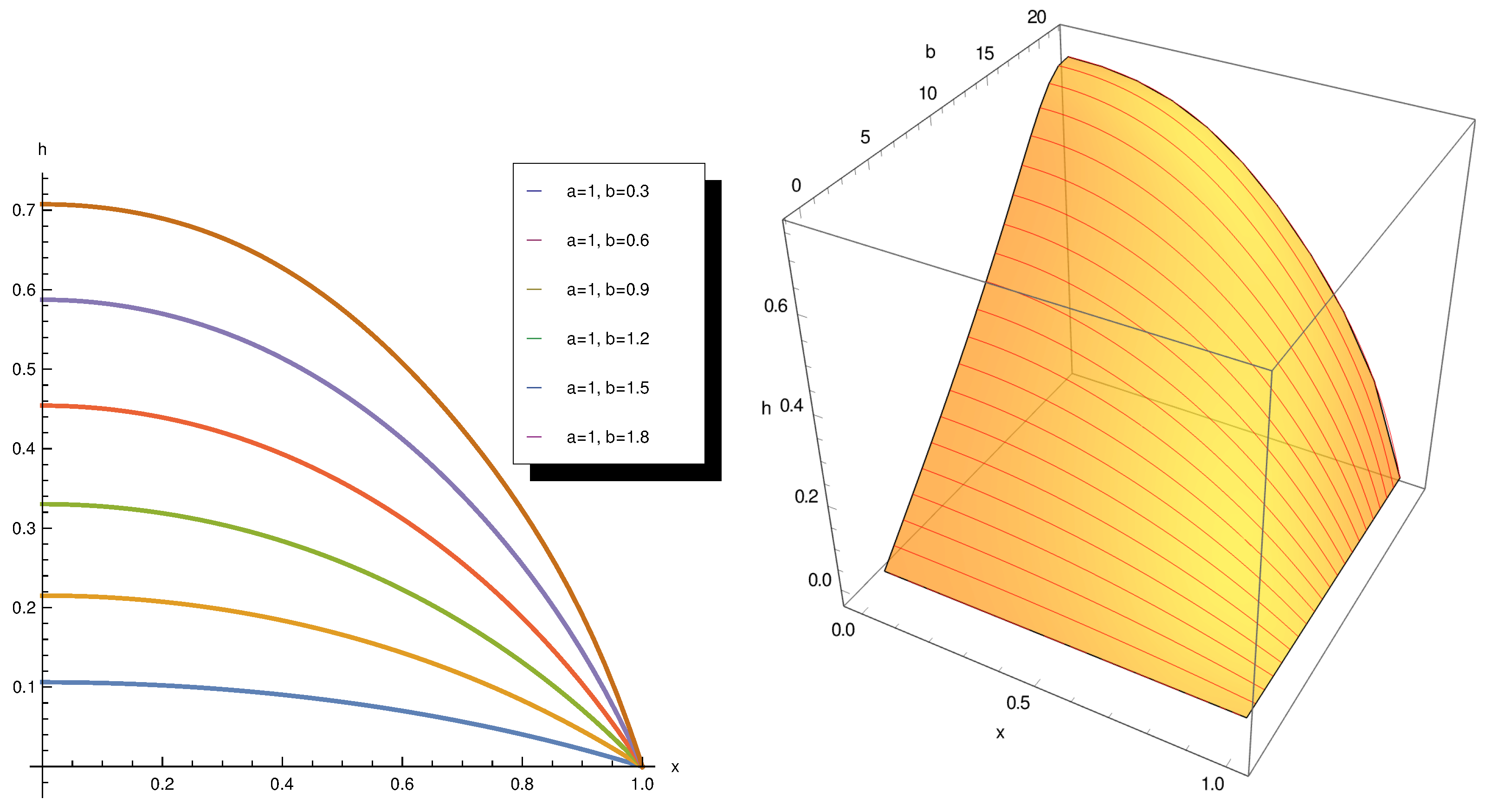
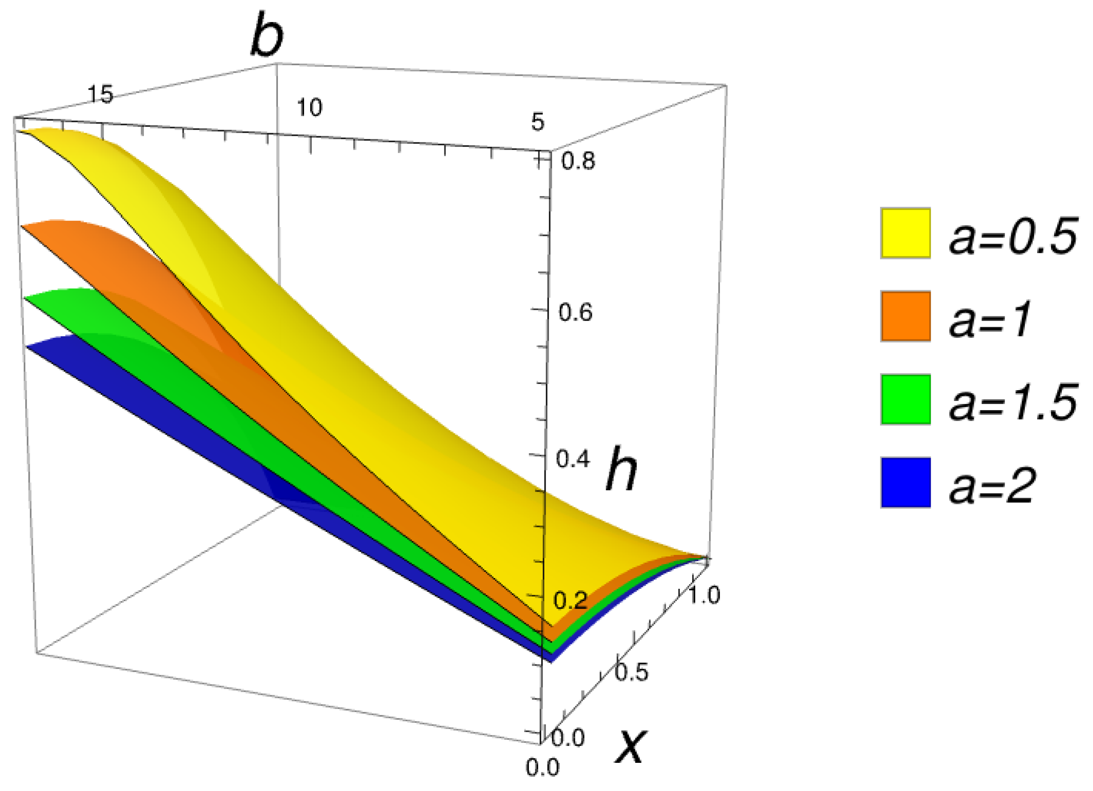
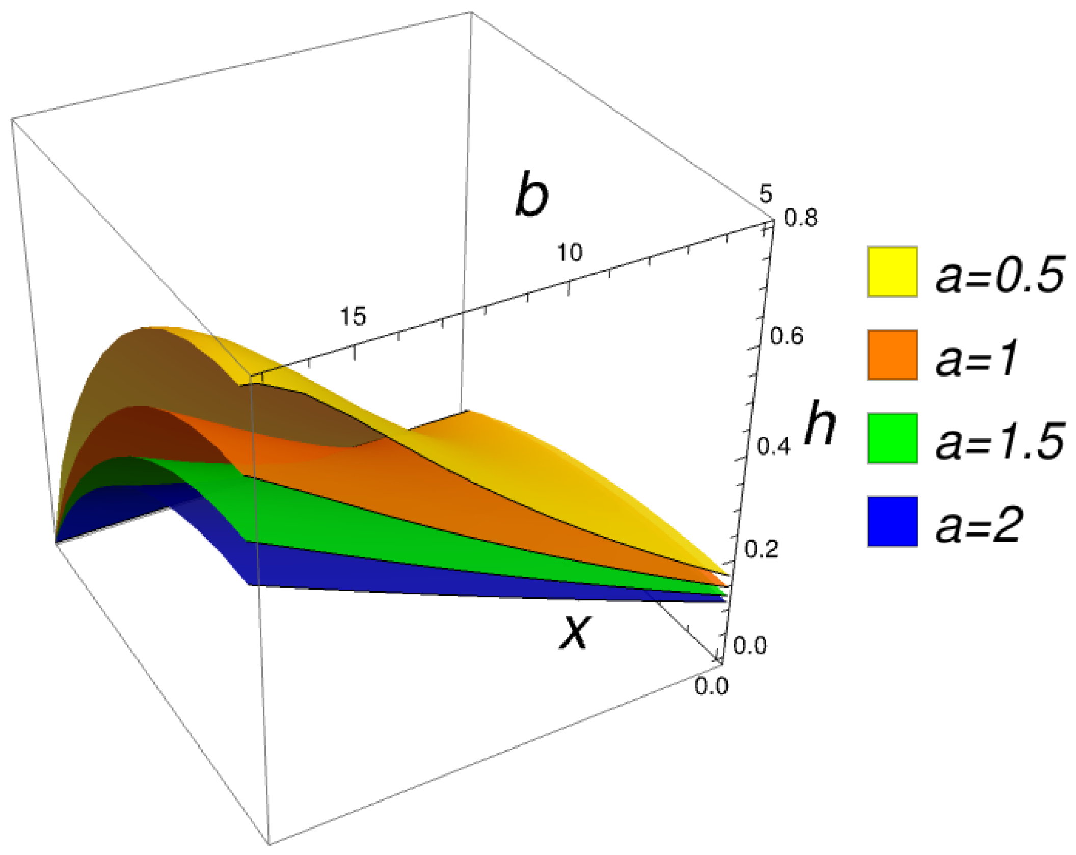
Even though the variables a and b are non-dimensionalized, by using the HPMLS approximations we can still visualize the influence of these parameters on the shape of the cornea. For example, since b is directly proportional to the intraocular pressure P, the following Figure 6, Figure 7, Figure 8 and Figure 9, which present the influence of b on h for different values of a, may also provide insight into the influence of the intraocular tension on the corneal shape.
The combined influence of a and b on the corneal shape can be visualized in Figure 10 and Figure 11. The results are in good concordance with real-world situation assessments [11], namely, values of a around 2.0 and b around 0.5 correlate with low intraocular pressure caused (hypotony), which in turn correlates with lower values of h; values of a around 1.7 and b around 1.6 correlate with normal intraocular pressure; and values of a around 0.5 and b around 2 correlate with high intraocular pressure (glaucoma), which in turn correlates with higher values of h.

5. Conclusions

In this paper the Homotopy Perturbation Method in conjunction with the Least Squares Method is used to calculate new and more accurate approximate analytical solutions for a nonlinear model of corneal curvature.
For the partially linearized model, the comparison with previous approximate solutions computed by other well-known methods illustrates the superior accuracy of HPMLS.
For the fully nonlinear model, for the first time very precise approximate analytical solutions are computed by HPMLS, and, by means of these approximations, a brief discussion on the influence of the parameters of the model on the solution is presented.

Author Contributions

All authors contributed to material preparation, data collection and analysis. All authors have read and agreed to the published version of the manuscript.

Funding

This research received no external funding.

Data Availability Statement

The original contributions presented in this study are included in the article. Further inquiries can be directed to the corresponding author.

Conflicts of Interest

The authors declare no conflicts of interest.

References

  1. Kasprzak, H.; Iskander, D.R. Approximating ocular surfaces by generalized conic curves. Opthalmic Physiol. Opt. 2006, 26, 602–609. [Google Scholar] [CrossRef] [PubMed]
  2. Rosales, M.A.; Jurez-Aubry, M.; Lpez-Olazagasti, E.; Ibarra, J.; Tepichn, E. Anterior corneal profile with variable asphericity. Appl. Opt. 2009, 48, 6594–6599. [Google Scholar] [CrossRef] [PubMed]
  3. Anderson, K.; El-Sheikh, A.; Newson, T. Application of structural analysis to the mechanical behaviour of the cornea. J. R. Soc. Interface 2004, 1, 3–15. [Google Scholar] [CrossRef] [PubMed]
  4. Ahmed, E. Finite element modeling of corneal biomechanical behavior. J. Refract. Surg. 2010, 26, 289–300. [Google Scholar] [CrossRef] [PubMed]
  5. Iskander, D.R.; Collins, M.J.; Davis, B. Optimal modeling of corneal surfaces by Zernike polynomials. IEEE Trans. Biomed. Eng. 2001, 48, 87–95. [Google Scholar] [CrossRef] [PubMed]
  6. Urs, R.; Ho, A.; Manns, F.; Parel, J.M. Age dependent Fourier model of the shape of the isolated ex vivo human crystalline lens. Vis. Res. 2010, 50, 1041–1047. [Google Scholar] [CrossRef] [PubMed]
  7. Ertürk, V.S.; Ahmadkhanlu, A.; Kumar, P.; Govindaraj, V. Some novel mathematical analysis on a corneal shape model by using Caputo fractional derivative. Optik 2022, 261, 169086. [Google Scholar] [CrossRef]
  8. Okrasiński, W.; Płociniczak, Ł. A nonlinear mathematical model of the corneal shape. Nonlinear Anal. Real World Appl. 2012, 13, 1498–1505. [Google Scholar] [CrossRef]
  9. Coelho, I.; Corsato, C.; Omari, P. A one-dimensional prescribed curvature equation modeling the corneal shape. Bound. Value Probl. 2014, 2014, 127. [Google Scholar] [CrossRef]
  10. He, J.-H. A remark on “A nonlinear mathematical model of the corneal shape”. Nonlinear Anal. Real World Appl. 2012, 13, 2863–2865. [Google Scholar] [CrossRef]
  11. Moghadas, H. Approximate analytical solutions for a nonlinear differential equation of the corneal geometry. Inform. Med. Unlocked 2020, 20, 100410. [Google Scholar] [CrossRef]
  12. Płociniczak, Ł.; Okrasiński, W.; Nieto, J.J.; Domínguez, O. On a nonlinear boundary value problem modeling corneal shape. J. Math. Anal. Appl. 2014, 414, 461–471. [Google Scholar] [CrossRef]
  13. Abukhaled, M.; Khuri, S. An Efficient Semi-Analytical Solution of a One-Dimensional Curvature Equation that Describes the Human Corneal Shape. Math. Comput. Appl. 2019, 24, 8. [Google Scholar] [CrossRef]
  14. Abukhaled, M.; Abukhaled, Y. Efficient semianalytical investigation of a fractional model describing human cornea shape. Model. Artif. Intell. Ophthalmol. 2024, 6, 1–15. [Google Scholar] [CrossRef]
  15. Płociniczak, Ł.; Griffiths, G.W.; Schiesser, W.E. ODE/PDE analysis of corneal curvature. Comput. Biol. Med. 2014, 53, 30–41. [Google Scholar] [CrossRef] [PubMed]
  16. Bota, C.; Căruntu, B. Approximate analytical solutions of nonlinear differential equations using the Least Squares Homotopy Perturbation Method. J. Math. Anal. Appl. 2017, 448, 401–408. [Google Scholar] [CrossRef]
  17. Bota, C.; Căruntu, B.; Lăzureanu, C. The Least Square Homotopy Perturbation Method for Boundary Value Problems. Appl. Comput. Math. 2017, 16, 39–47. [Google Scholar]
  18. Paşca, M.; Bundău, O.; Juratoni, A.; Căruntu, B. The Least Squares Homotopy Perturbation Method for Systems of Differential Equations with Application to a Blood Flow Model. Mathematics 2022, 10, 546. [Google Scholar] [CrossRef]
  19. He, J.H. Homotopy perturbation technique, Computer Methods in Applied Mechanics and Engineering. Int. J. Nonlinear Mech. 1999, 178, 257–262. [Google Scholar] [CrossRef]
  20. He, J.H. An elementary introduction to the homotopy perturbation method. Comput. Math. Appl. 2009, 57, 410–412. [Google Scholar] [CrossRef]
  21. Ghasemi, M.; Babolian, E.; Saeidiain, J.; Azizi, A. A General Approach for Applying Homotopy Perturbation Method for Differential and Systems of Differential Equations. Aust. J. Basic Appl. Sci. 2011, 5, 3280–3294. [Google Scholar]
Figure 1. The modeled corneal geometry—the corneal section h ( x ) is the red curve.
Mathematics 14 02185 g001
Figure 2. Absolute errors of the best approximations for partially linearized model (right: full plot, left: detail).
Mathematics 14 02185 g002
Figure 3. Absolute errors of the approximations computed by HPMLS for the fully nonlinear model.
Mathematics 14 02185 g003
Figure 4. Absolute errors of the approximations computed by HPMLS for the fully nonlinear model (detail).
Mathematics 14 02185 g004
Figure 5. Absolute errors of the approximations computed by HPMLS for the fully nonlinear model (detail).
Mathematics 14 02185 g005
Figure 6. The influence of b on h for a = 0.5 .
Mathematics 14 02185 g006
Figure 7. The influence of b on h for a = 1 .
Mathematics 14 02185 g007
Figure 8. The influence of b on h for a = 1.5 .
Mathematics 14 02185 g008
Figure 9. The influence of b on h for a = 2 .
Mathematics 14 02185 g009
Figure 10. The combined influence of a and b on the corneal shape.
Mathematics 14 02185 g010
Figure 11. The combined influence of a and b on the corneal shape.
Mathematics 14 02185 g011
Table 1. Absolute errors of the approximations computed by regular HPM for the first homotopy.
x f 1 f 2 f 3 f 4 f 5 f 6 f 7
01.5933 × 10 1 4.8997 × 10 2 5.9417 × 10 3 1.5263 × 10 2 1.54473 × 10 4 1.2554 × 10 2 8.3762 × 10 3
0.11.5763 × 10 1 4.8203 × 10 2 6.1837 × 10 3 1.5232 × 10 2 7.7231 × 10 5 1.2555 × 10 2 8.3134 × 10 3
0.21.5253 × 10 1 4.5862 × 10 2 6.8734 × 10 3 1.5113 × 10 2 1.6476 × 10 4 1.2558 × 10 2 8.1228 × 10 3
0.31.4408 × 10 1 4.20876 × 10 2 7.9017 × 10 3 1.4838 × 10 2 5.9614 × 10 4 1.2562 × 10 2 7.7931 × 10 3
0.41.3233 × 10 1 3.7071 × 10 2 9.0869 × 10 3 1.4305 × 10 2 1.2374 × 10 3 1.2535 × 10 2 7.2898 × 10 3
0.51.1736 × 10 1 3.1071 × 10 2 1.0173 × 10 2 1.3386 × 10 2 2.0744 × 10 3 1.2395 × 10 2 6.5454 × 10 3
0.69.9311 × 10 2 2.4422 × 10 2 1.0831 × 10 2 1.1955 × 10 2 3.0157 × 10 3 1.1970 × 10 2 5.4672 × 10 3
0.77.8324 × 10 2 1.7513 × 10 2 1.0656 × 10 2 9.9062 × 10 3 3.8391 × 10 3 1.0975 × 10 2 3.9876 × 10 3
0.85.4602 × 10 2 1.0797 × 10 2 9.1722 × 10 3 7.1869 × 10 3 4.1272 × 10 3 8.9988 × 10 3 2.1812 × 10 3
0.92.8394 × 10 2 4.7761 × 10 3 5.8273 × 10 3 3.8315 × 10 3 3.1933 × 10 3 5.5258 × 10 3 4.7771 × 10 4
10.00000.00000.00000.00000.00000.00000.0000
Table 2. Absolute errors of the approximations computed by HPMLS for the first homotopy.
x h ˜ 1 h ˜ 2 h ˜ 3 h ˜ 4 h ˜ 5 h ˜ 6 h ˜ 7
08.7055 × 10 3 2.0047 × 10 4 4.5473 × 10 6 3.7955 × 10 7 3.1077 × 10 9 1.9917 × 10 9 2.2148 × 10 9
0.18.5094 × 10 3 1.8216 × 10 4 3.6061 × 10 6 2.9148 × 10 7 4.4043 × 10 9 2.2746 × 10 9 2.2262 × 10 9
0.27.9325 × 10 3 1.3108 × 10 4 1.1703 × 10 6 9.3061 × 10 8 1.9464 × 10 8 2.7426 × 10 9 2.2624 × 10 9
0.37.0095 × 10 3 5.8131 × 10 5 1.7508 × 10 6 6.4153 × 10 8 2.7535 × 10 8 2.9522 × 10 9 2.3152 × 10 9
0.45.8003 × 10 3 2.0656 × 10 5 3.9391 × 10 6 5.2347 × 10 8 2.2623 × 10 8 3.2636 × 10 9 2.3844 × 10 9
0.54.3929 × 10 3 8.7116 × 10 5 4.4938 × 10 6 1.2919 × 10 7 1.3645 × 10 8 4.1512 × 10 9 2.5024 × 10 9
0.62.9080 × 10 3 1.2490 × 10 4 3.2807 × 10 6 3.3363 × 10 7 1.2255 × 10 8 4.9443 × 10 9 2.6274 × 10 9
0.71.5026 × 10 3 1.2412 × 10 4 1.0911 × 10 6 3.6773 × 10 7 1.3747 × 10 8 5.0148 × 10 9 2.6697 × 10 9
0.83.7596 × 10 4 8.6527 × 10 5 6.5941 × 10 7 1.7569 × 10 7 2.7923 × 10 10 6.3557 × 10 9 3.0137 × 10 9
0.92.2504 × 10 4 3.1098 × 10 5 8.1476 × 10 7 3.7647 × 10 8 2.2252 × 10 8 8.8109 × 10 9 3.6056 × 10 9
10.00000.00000.00000.00000.00000.00000.0000
Table 3. Absolute errors of the approximations computed by HPM ( f n ) and HPMLS ( h ˜ n ) for the second homotopy.
x f 3 h ˜ 3 f 5 h ˜ 5 f 7 h ˜ 7
06.7923 × 10 1 5.4339 × 10 4 6.7539 × 10 4 1.4011 × 10 8 2.8912 × 10 4 1.0681 × 10 8
0.16.7262 × 10 1 5.0511 × 10 4 6.7879 × 10 4 2.5516 × 10 9 2.9057 × 10 4 1.0735 × 10 8
0.26.5278 × 10 1 3.9745 × 10 4 6.8914 × 10 4 3.6068 × 10 8 2.9498 × 10 4 1.0904 × 10 8
0.36.1964 × 10 1 2.4103 × 10 4 7.0699 × 10 4 5.4445 × 10 8 3.0254 × 10 4 1.1163 × 10 8
0.45.7307 × 10 1 6.6777 × 10 5 7.3313 × 10 4 4.3107 × 10 8 3.1365 × 10 4 1.1510 × 10 8
0.55.1292 × 10 1 8.9108 × 10 5 7.6731 × 10 4 2.0737 × 10 8 3.2882 × 10 4 1.2051 × 10 8
0.64.3899 × 10 1 1.9211 × 10 4 8.0471 × 10 4 1.4926 × 10 8 3.4806 × 10 4 1.2643 × 10 8
0.73.5102 × 10 1 2.1829 × 10 4 8.2759 × 10 4 1.7781 × 10 8 3.6766 × 10 4 1.2963 × 10 8
0.82.4874 × 10 1 1.6517 × 10 4 7.8911 × 10 4 1.4012 × 10 8 3.7041 × 10 4 1.4504 × 10 8
0.91.3184 × 10 1 6.4892 × 10 5 5.8413 × 10 4 6.4981 × 10 8 2.9988 × 10 4 1.7003 × 10 8
10.00000.00000.00000.00000.00000.0000
Table 4. Comparison of the relative errors of the approximations computed by HPMLS and other methods.
x h ˜ 7 H 1 h ˜ 7 H 2 h res [14] h gre [13] h tay   [13] h lin [13] h hcs [13] h per [13]
06.50167 × 10 7 3.1353 × 10 6 4.9666 × 10 4 5.0 × 10 5 3.2318 × 10 1 3.233153.311779.93049
0.16.5990 × 10 7 3.1821 × 10 6 5.0417 × 10 4 2.0 × 10 5 3.2800 × 10 1 3.271783.360319.97343
0.26.9091 × 10 7 3.3300 × 10 6 5.2762 × 10 4 4.0 × 10 5 3.4291 × 10 1 3.358773.505571.0102 × 10 1
0.37.4464 × 10 7 3.5903 × 10 6 5.7007 × 10 4 5.0 × 10 5 3.6958 × 10 1 3.462623.746151.0314 × 10 1
0.48.2887 × 10 7 4.0011 × 10 6 6.3783 × 10 4 5.0 × 10 5 4.1066 × 10 1 3.562954.079851.0607 × 10 1
0.59.7131 × 10 7 4.6776 × 10 6 7.4325 × 10 4 5.0 × 10 5 4.6910 × 10 1 3.646954.503751.0977 × 10 1
0.61.1905 × 10 6 5.7291 × 10 6 9.1159 × 10 4 5.0 × 10 5 5.5066 × 10 1 3.707075.014261.1421 × 10 1
0.71.5111 × 10 6 7.3374 × 10 6 1.1988 × 10 3 4.0 × 10 5 6.5862 × 10 1 3.739515.607231.1933 × 10 1
0.82.4033 × 10 6 1.1567 × 10 5 1.7383 × 10 3 7.0 × 10 5 7.9862 × 10 1 3.743046.278161.2506 × 10 1
0.95.4134 × 10 6 2.5528 × 10 5 2.8505 × 10 3 1.8 × 10 4 9.7608 × 10 1 3.718367.022181.3136 × 10 1
Table 5. The percentage improvement of h ˜ 7 H 1 over the previous approximations.
h res [14] h gre [13] h tay [13] h lin [13] h hcs [13] h per [13]
99.8631197.5983599.9997499.9999599.9999799.99998
Table 6. Absolute errors of the approximations computed by HPMLS for the fully nonlinear model.
x h ˜ 3 h ˜ 4 h ˜ 5 h ˜ 6 h ˜ 7
01.5438 × 10 5 6.8967 × 10 5 1.6427 × 10 6 2.0665 × 10 6 1.4717 × 10 6
0.16.2002 × 10 5 5.6995 × 10 5 7.6261 × 10 8 2.1495 × 10 6 1.4792 × 10 6
0.22.6749 × 10 4 2.9233 × 10 5 3.1338 × 10 6 2.3001 × 10 6 1.5025 × 10 6
0.35.2767 × 10 4 5.3981 × 10 6 4.9418 × 10 6 2.3981 × 10 6 1.5399 × 10 6
0.47.4338 × 10 4 4.4524 × 10 6 3.7909 × 10 6 2.5414 × 10 6 1.5927 × 10 6
0.58.2158 × 10 4 3.0376 × 10 5 1.3736 × 10 6 2.8836 × 10 6 1.6743 × 10 6
0.67.1374 × 10 4 6.4426 × 10 5 6.3452 × 10 7 3.2354 × 10 6 1.7732 × 10 6
0.74.5111 × 10 4 7.3040 × 10 5 9.1036 × 10 7 3.3710 × 10 6 1.8557 × 10 6
0.81.5823 × 10 4 3.6508 × 10 5 3.3159 × 10 6 4.1047 × 10 6 2.1133 × 10 6
0.94.5879 × 10 6 1.2438 × 10 5 1.0892 × 10 5 5.4858 × 10 6 2.5499 × 10 6
Disclaimer/Publisher’s Note: The statements, opinions and data contained in all publications are solely those of the individual author(s) and contributor(s) and not of MDPI and/or the editor(s). MDPI and/or the editor(s) disclaim responsibility for any injury to people or property resulting from any ideas, methods, instructions or products referred to in the content.