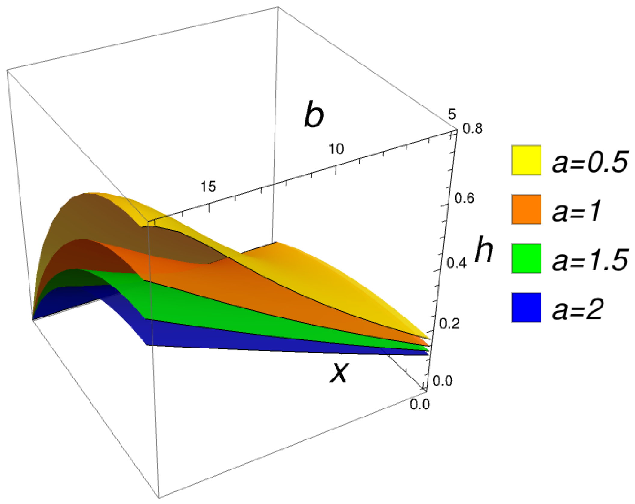
Approximate Analytical Solutions for a Nonlinear Model of Corneal Curvature Using the Homotopy Perturbation Method in Conjunction with the Least Squares Method



Abstract
1. Introduction
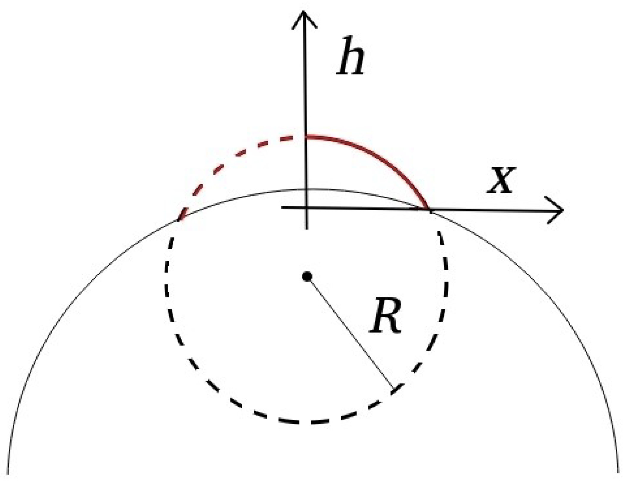
- R is the radius of the corneal section
- P is the intraocular pressure acting in a normal direction to the cross-section of cornea
- T is the tension acting tangentially
- k is the elastic constant of the spring force proportional to h (introduced to model the elastic features of the cornea)
- Accelerated convergence compared to the regular HPM and most other similar methods.
- Very accurate approximate analytical solutions.
- Possible application for problems defined on wide (even infinite) intervals for the variables.
- Possible application to a wide range of nonlinear problems (ODEs, PDEs, integro-differential equations, optimal problems, etc.).
2. Homotopy Perturbation Method in Conjunction with the Least Squares Method (HPMLS)
- is a linear differential operator, chosen in such a way that the problem is easily solvable and, if possible, characterizes the dominant behavior of the system.
- is a nonlinear operator that represents the rest of the problem (such that ).
- By imposing the boundary conditions, we can determine , such that are computed as functions of .
- We substitute the approximate solution in the initial equation and obtain the expression:
- We attach to the problem the following real functional:
- We compute the values of as the values that give the minimum of the functional (14) and the values of again as functions of by using the boundary conditions.
- Using the constants thus determined, we consider the HP-sequence:
3. Numerical Results for the Partially Linearized Model
3.1. Homotopy No. 1
3.2. Homotopy No. 2
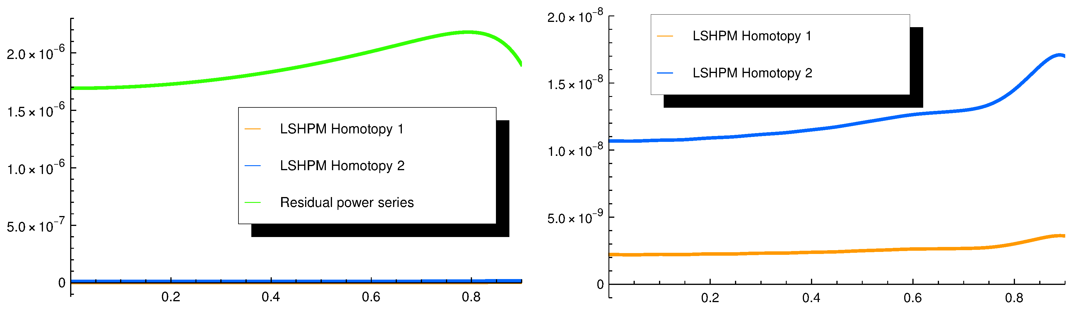
3.3. Comparison with Previous Results
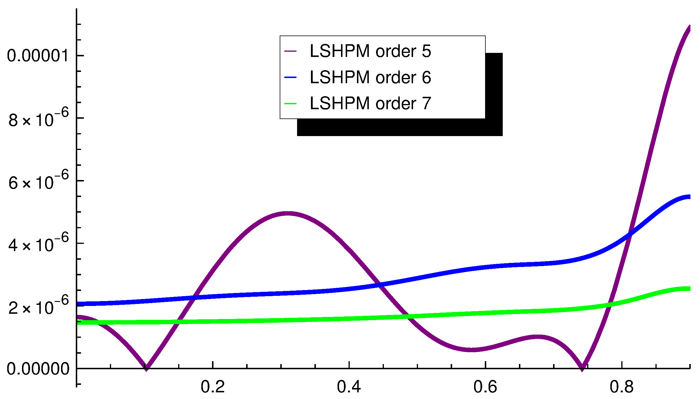
- The seventh-order approximations computed by HPMLS in the previous sections by means of the two homotopies. Thus denotes the polynomial approximation obtained by means of the first homotopy, while denotes the approximation consisting of hyperbolic functions obtained by means of the second homotopy.
- Green’s function method based approximation [13], denoted by .
- Approximation by the residual power series method [14], denoted by .
4. Numerical Results for the Fully Nonlinear Model
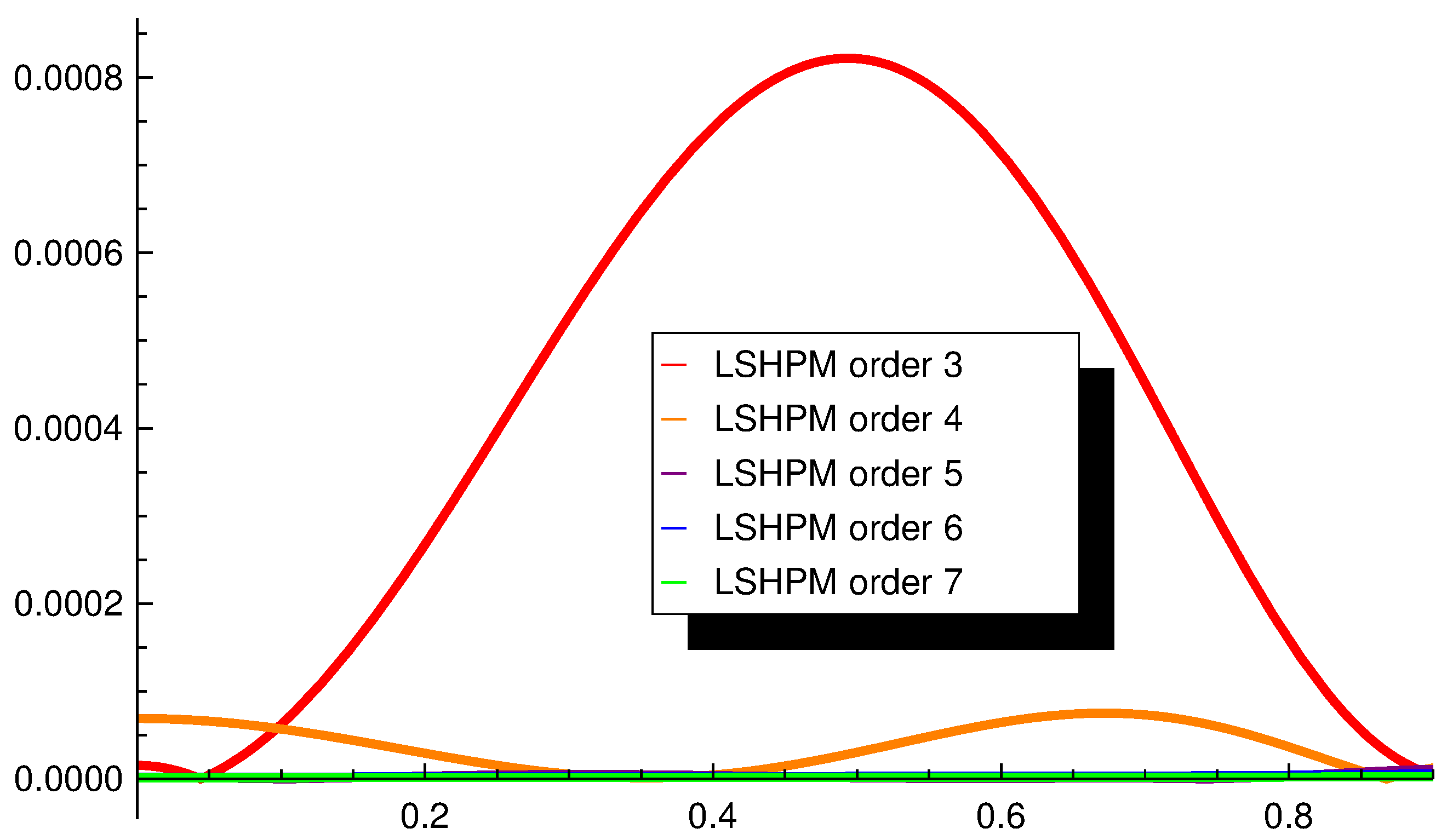
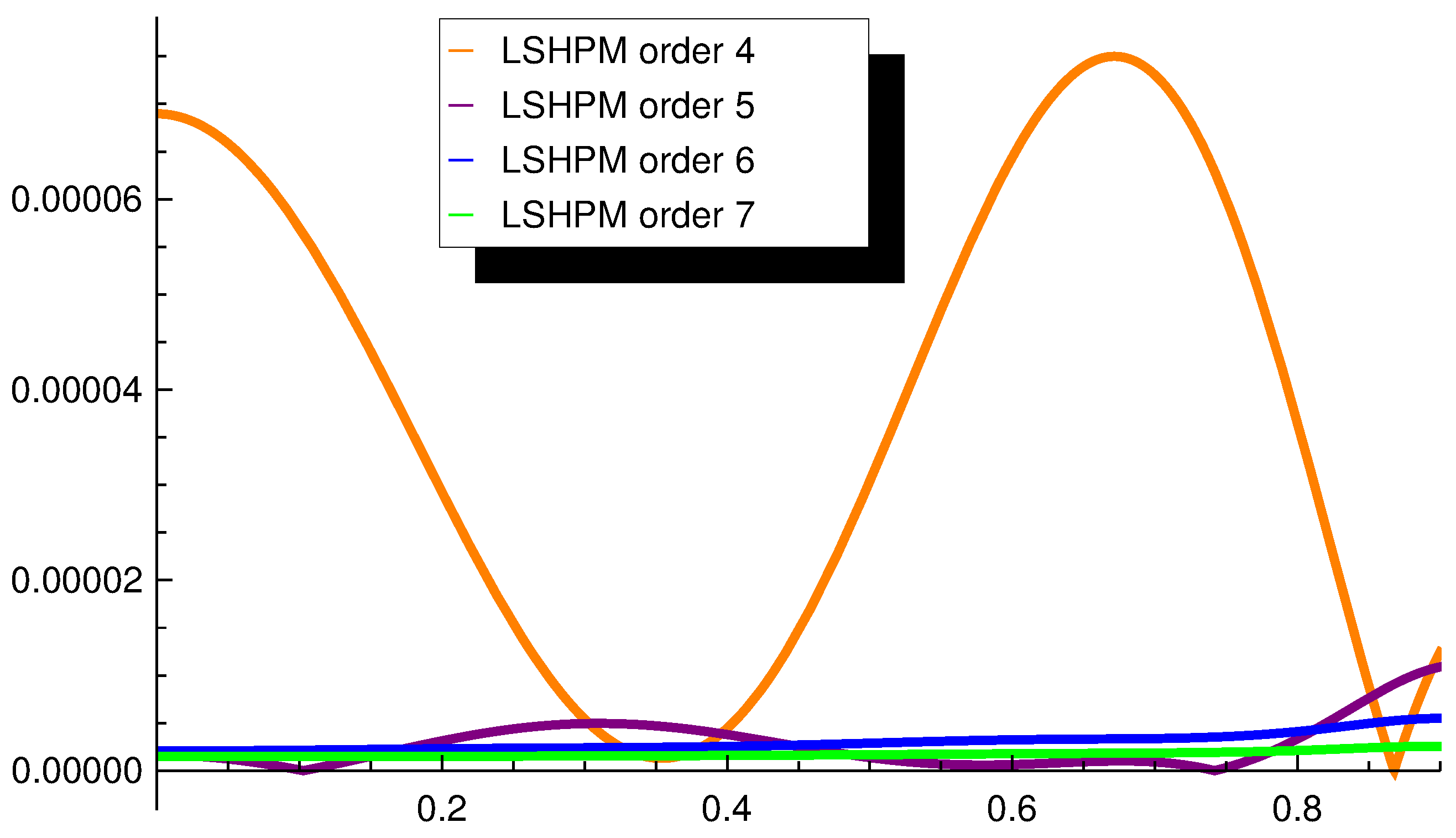
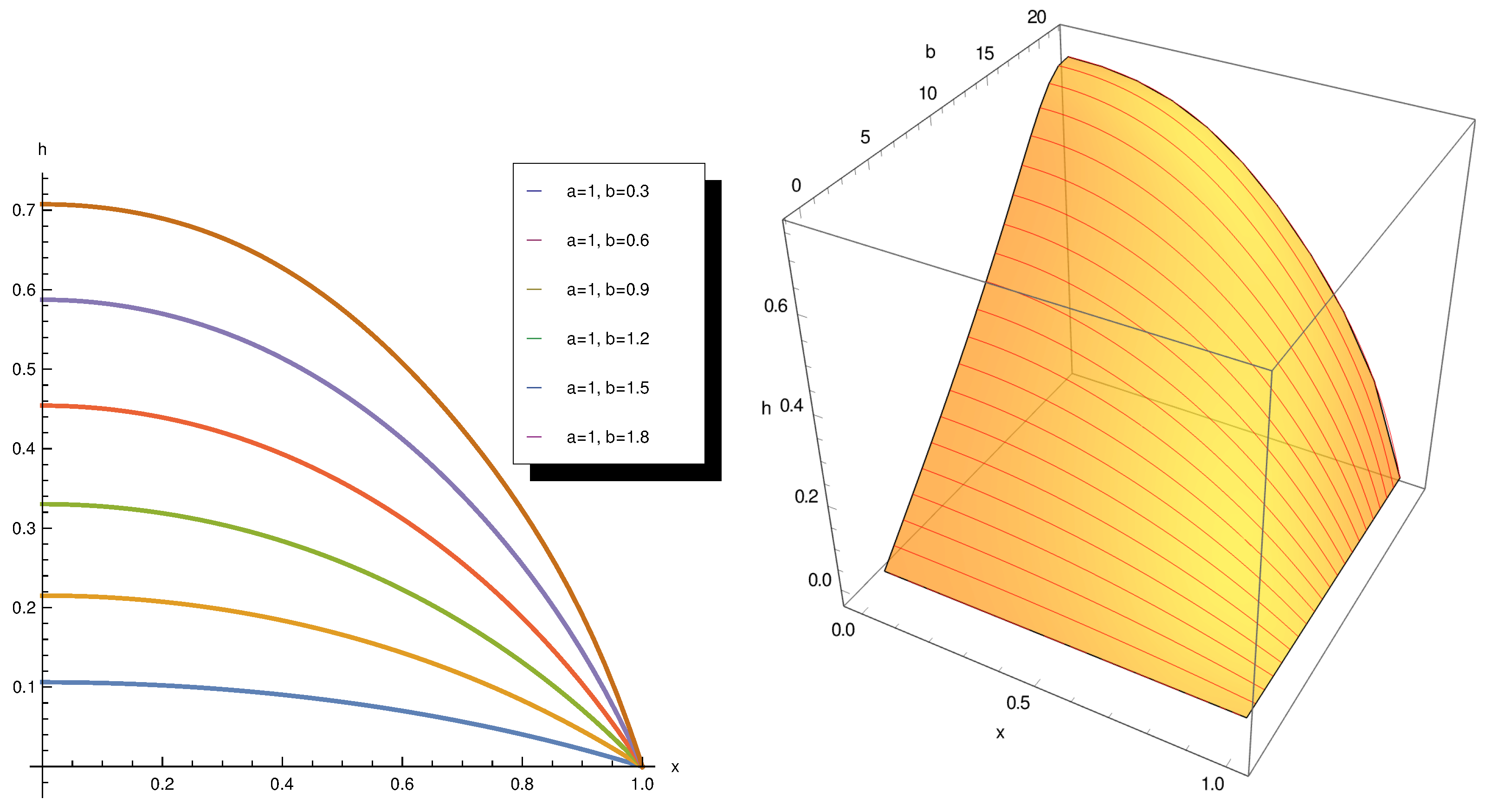
4.1. HPMLS Approximations
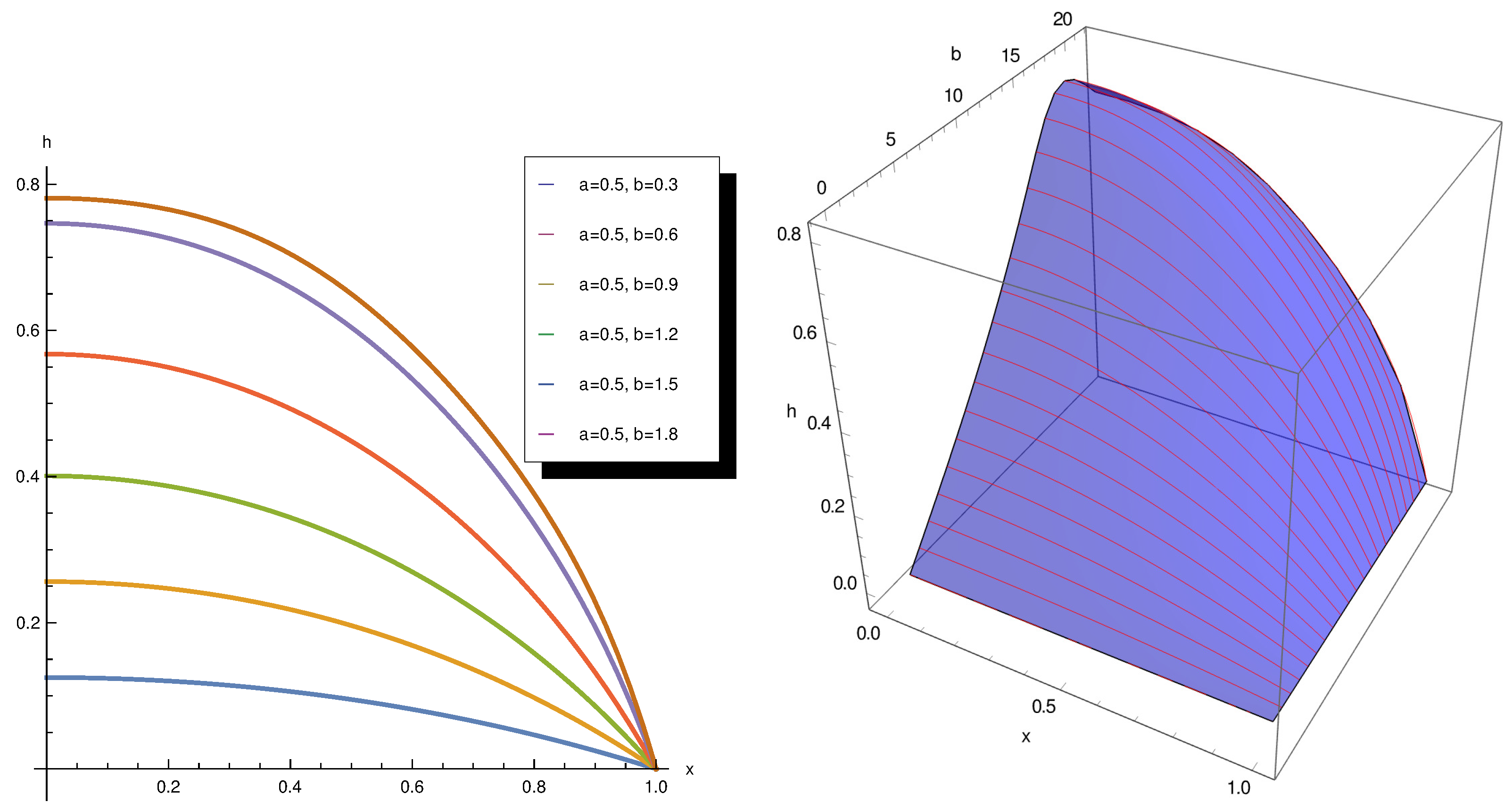
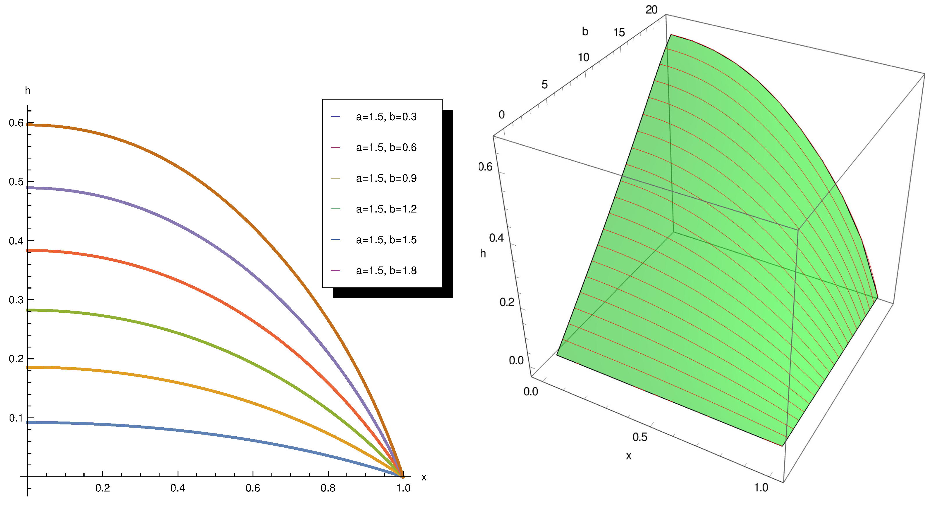
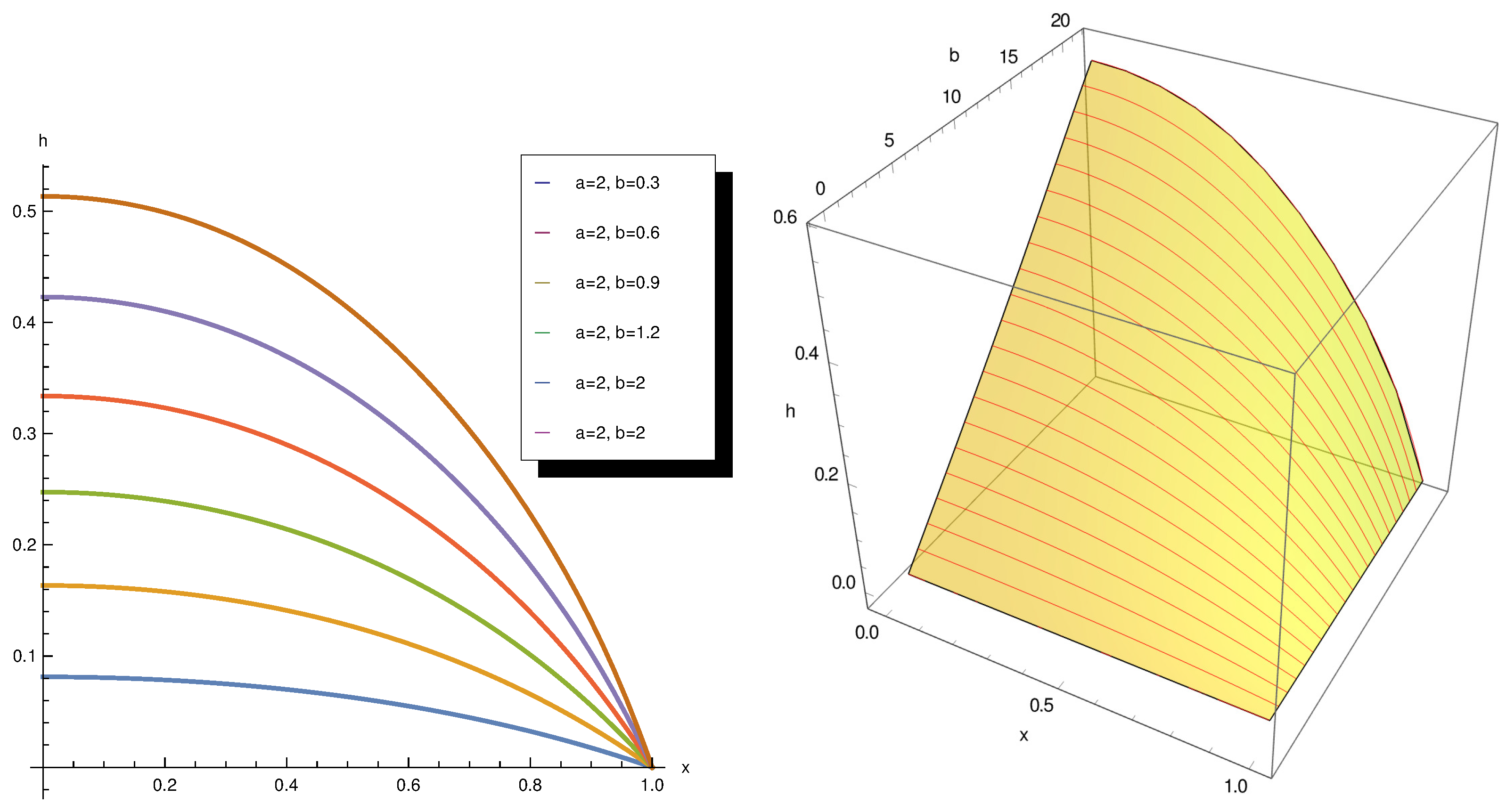
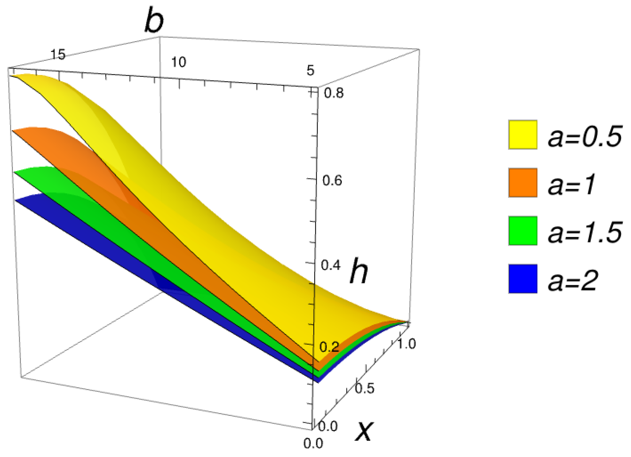
4.2. Discussion
5. Conclusions
Author Contributions
Funding
Data Availability Statement
Conflicts of Interest
References
- Kasprzak, H.; Iskander, D.R. Approximating ocular surfaces by generalized conic curves. Opthalmic Physiol. Opt. 2006, 26, 602–609. [Google Scholar] [CrossRef] [PubMed]
- Rosales, M.A.; Jurez-Aubry, M.; Lpez-Olazagasti, E.; Ibarra, J.; Tepichn, E. Anterior corneal profile with variable asphericity. Appl. Opt. 2009, 48, 6594–6599. [Google Scholar] [CrossRef] [PubMed]
- Anderson, K.; El-Sheikh, A.; Newson, T. Application of structural analysis to the mechanical behaviour of the cornea. J. R. Soc. Interface 2004, 1, 3–15. [Google Scholar] [CrossRef] [PubMed]
- Ahmed, E. Finite element modeling of corneal biomechanical behavior. J. Refract. Surg. 2010, 26, 289–300. [Google Scholar] [CrossRef] [PubMed]
- Iskander, D.R.; Collins, M.J.; Davis, B. Optimal modeling of corneal surfaces by Zernike polynomials. IEEE Trans. Biomed. Eng. 2001, 48, 87–95. [Google Scholar] [CrossRef] [PubMed]
- Urs, R.; Ho, A.; Manns, F.; Parel, J.M. Age dependent Fourier model of the shape of the isolated ex vivo human crystalline lens. Vis. Res. 2010, 50, 1041–1047. [Google Scholar] [CrossRef] [PubMed]
- Ertürk, V.S.; Ahmadkhanlu, A.; Kumar, P.; Govindaraj, V. Some novel mathematical analysis on a corneal shape model by using Caputo fractional derivative. Optik 2022, 261, 169086. [Google Scholar] [CrossRef]
- Okrasiński, W.; Płociniczak, Ł. A nonlinear mathematical model of the corneal shape. Nonlinear Anal. Real World Appl. 2012, 13, 1498–1505. [Google Scholar] [CrossRef]
- Coelho, I.; Corsato, C.; Omari, P. A one-dimensional prescribed curvature equation modeling the corneal shape. Bound. Value Probl. 2014, 2014, 127. [Google Scholar] [CrossRef]
- He, J.-H. A remark on “A nonlinear mathematical model of the corneal shape”. Nonlinear Anal. Real World Appl. 2012, 13, 2863–2865. [Google Scholar] [CrossRef]
- Moghadas, H. Approximate analytical solutions for a nonlinear differential equation of the corneal geometry. Inform. Med. Unlocked 2020, 20, 100410. [Google Scholar] [CrossRef]
- Płociniczak, Ł.; Okrasiński, W.; Nieto, J.J.; Domínguez, O. On a nonlinear boundary value problem modeling corneal shape. J. Math. Anal. Appl. 2014, 414, 461–471. [Google Scholar] [CrossRef]
- Abukhaled, M.; Khuri, S. An Efficient Semi-Analytical Solution of a One-Dimensional Curvature Equation that Describes the Human Corneal Shape. Math. Comput. Appl. 2019, 24, 8. [Google Scholar] [CrossRef]
- Abukhaled, M.; Abukhaled, Y. Efficient semianalytical investigation of a fractional model describing human cornea shape. Model. Artif. Intell. Ophthalmol. 2024, 6, 1–15. [Google Scholar] [CrossRef]
- Płociniczak, Ł.; Griffiths, G.W.; Schiesser, W.E. ODE/PDE analysis of corneal curvature. Comput. Biol. Med. 2014, 53, 30–41. [Google Scholar] [CrossRef] [PubMed]
- Bota, C.; Căruntu, B. Approximate analytical solutions of nonlinear differential equations using the Least Squares Homotopy Perturbation Method. J. Math. Anal. Appl. 2017, 448, 401–408. [Google Scholar] [CrossRef]
- Bota, C.; Căruntu, B.; Lăzureanu, C. The Least Square Homotopy Perturbation Method for Boundary Value Problems. Appl. Comput. Math. 2017, 16, 39–47. [Google Scholar]
- Paşca, M.; Bundău, O.; Juratoni, A.; Căruntu, B. The Least Squares Homotopy Perturbation Method for Systems of Differential Equations with Application to a Blood Flow Model. Mathematics 2022, 10, 546. [Google Scholar] [CrossRef]
- He, J.H. Homotopy perturbation technique, Computer Methods in Applied Mechanics and Engineering. Int. J. Nonlinear Mech. 1999, 178, 257–262. [Google Scholar] [CrossRef]
- He, J.H. An elementary introduction to the homotopy perturbation method. Comput. Math. Appl. 2009, 57, 410–412. [Google Scholar] [CrossRef]
- Ghasemi, M.; Babolian, E.; Saeidiain, J.; Azizi, A. A General Approach for Applying Homotopy Perturbation Method for Differential and Systems of Differential Equations. Aust. J. Basic Appl. Sci. 2011, 5, 3280–3294. [Google Scholar]






| x | |||||||
|---|---|---|---|---|---|---|---|
| 0 | 1.5933 | 4.8997 | 5.9417 | 1.5263 | 1.54473 | 1.2554 | 8.3762 |
| 0.1 | 1.5763 | 4.8203 | 6.1837 | 1.5232 | 7.7231 | 1.2555 | 8.3134 |
| 0.2 | 1.5253 | 4.5862 | 6.8734 | 1.5113 | 1.6476 | 1.2558 | 8.1228 |
| 0.3 | 1.4408 | 4.20876 | 7.9017 | 1.4838 | 5.9614 | 1.2562 | 7.7931 |
| 0.4 | 1.3233 | 3.7071 | 9.0869 | 1.4305 | 1.2374 | 1.2535 | 7.2898 |
| 0.5 | 1.1736 | 3.1071 | 1.0173 | 1.3386 | 2.0744 | 1.2395 | 6.5454 |
| 0.6 | 9.9311 | 2.4422 | 1.0831 | 1.1955 | 3.0157 | 1.1970 | 5.4672 |
| 0.7 | 7.8324 | 1.7513 | 1.0656 | 9.9062 | 3.8391 | 1.0975 | 3.9876 |
| 0.8 | 5.4602 | 1.0797 | 9.1722 | 7.1869 | 4.1272 | 8.9988 | 2.1812 |
| 0.9 | 2.8394 | 4.7761 | 5.8273 | 3.8315 | 3.1933 | 5.5258 | 4.7771 |
| 1 | 0.0000 | 0.0000 | 0.0000 | 0.0000 | 0.0000 | 0.0000 | 0.0000 |
| x | |||||||
|---|---|---|---|---|---|---|---|
| 0 | 8.7055 | 2.0047 | 4.5473 | 3.7955 | 3.1077 | 1.9917 | 2.2148 |
| 0.1 | 8.5094 | 1.8216 | 3.6061 | 2.9148 | 4.4043 | 2.2746 | 2.2262 |
| 0.2 | 7.9325 | 1.3108 | 1.1703 | 9.3061 | 1.9464 | 2.7426 | 2.2624 |
| 0.3 | 7.0095 | 5.8131 | 1.7508 | 6.4153 | 2.7535 | 2.9522 | 2.3152 |
| 0.4 | 5.8003 | 2.0656 | 3.9391 | 5.2347 | 2.2623 | 3.2636 | 2.3844 |
| 0.5 | 4.3929 | 8.7116 | 4.4938 | 1.2919 | 1.3645 | 4.1512 | 2.5024 |
| 0.6 | 2.9080 | 1.2490 | 3.2807 | 3.3363 | 1.2255 | 4.9443 | 2.6274 |
| 0.7 | 1.5026 | 1.2412 | 1.0911 | 3.6773 | 1.3747 | 5.0148 | 2.6697 |
| 0.8 | 3.7596 | 8.6527 | 6.5941 | 1.7569 | 2.7923 | 6.3557 | 3.0137 |
| 0.9 | 2.2504 | 3.1098 | 8.1476 | 3.7647 | 2.2252 | 8.8109 | 3.6056 |
| 1 | 0.0000 | 0.0000 | 0.0000 | 0.0000 | 0.0000 | 0.0000 | 0.0000 |
| x | ||||||
|---|---|---|---|---|---|---|
| 0 | 6.7923 | 5.4339 | 6.7539 | 1.4011 | 2.8912 | 1.0681 |
| 0.1 | 6.7262 | 5.0511 | 6.7879 | 2.5516 | 2.9057 | 1.0735 |
| 0.2 | 6.5278 | 3.9745 | 6.8914 | 3.6068 | 2.9498 | 1.0904 |
| 0.3 | 6.1964 | 2.4103 | 7.0699 | 5.4445 | 3.0254 | 1.1163 |
| 0.4 | 5.7307 | 6.6777 | 7.3313 | 4.3107 | 3.1365 | 1.1510 |
| 0.5 | 5.1292 | 8.9108 | 7.6731 | 2.0737 | 3.2882 | 1.2051 |
| 0.6 | 4.3899 | 1.9211 | 8.0471 | 1.4926 | 3.4806 | 1.2643 |
| 0.7 | 3.5102 | 2.1829 | 8.2759 | 1.7781 | 3.6766 | 1.2963 |
| 0.8 | 2.4874 | 1.6517 | 7.8911 | 1.4012 | 3.7041 | 1.4504 |
| 0.9 | 1.3184 | 6.4892 | 5.8413 | 6.4981 | 2.9988 | 1.7003 |
| 1 | 0.0000 | 0.0000 | 0.0000 | 0.0000 | 0.0000 | 0.0000 |
| x | [14] | [13] | [13] | [13] | [13] | [13] | ||
|---|---|---|---|---|---|---|---|---|
| 0 | 6.50167 | 3.1353 | 4.9666 | 5.0 | 3.2318 | 3.23315 | 3.31177 | 9.93049 |
| 0.1 | 6.5990 | 3.1821 | 5.0417 | 2.0 | 3.2800 | 3.27178 | 3.36031 | 9.97343 |
| 0.2 | 6.9091 | 3.3300 | 5.2762 | 4.0 | 3.4291 | 3.35877 | 3.50557 | 1.0102 |
| 0.3 | 7.4464 | 3.5903 | 5.7007 | 5.0 | 3.6958 | 3.46262 | 3.74615 | 1.0314 |
| 0.4 | 8.2887 | 4.0011 | 6.3783 | 5.0 | 4.1066 | 3.56295 | 4.07985 | 1.0607 |
| 0.5 | 9.7131 | 4.6776 | 7.4325 | 5.0 | 4.6910 | 3.64695 | 4.50375 | 1.0977 |
| 0.6 | 1.1905 | 5.7291 | 9.1159 | 5.0 | 5.5066 | 3.70707 | 5.01426 | 1.1421 |
| 0.7 | 1.5111 | 7.3374 | 1.1988 | 4.0 | 6.5862 | 3.73951 | 5.60723 | 1.1933 |
| 0.8 | 2.4033 | 1.1567 | 1.7383 | 7.0 | 7.9862 | 3.74304 | 6.27816 | 1.2506 |
| 0.9 | 5.4134 | 2.5528 | 2.8505 | 1.8 | 9.7608 | 3.71836 | 7.02218 | 1.3136 |
| [14] | [13] | [13] | [13] | [13] | [13] |
|---|---|---|---|---|---|
| 99.86311 | 97.59835 | 99.99974 | 99.99995 | 99.99997 | 99.99998 |
| x | |||||
|---|---|---|---|---|---|
| 0 | 1.5438 | 6.8967 | 1.6427 | 2.0665 | 1.4717 |
| 0.1 | 6.2002 | 5.6995 | 7.6261 | 2.1495 | 1.4792 |
| 0.2 | 2.6749 | 2.9233 | 3.1338 | 2.3001 | 1.5025 |
| 0.3 | 5.2767 | 5.3981 | 4.9418 | 2.3981 | 1.5399 |
| 0.4 | 7.4338 | 4.4524 | 3.7909 | 2.5414 | 1.5927 |
| 0.5 | 8.2158 | 3.0376 | 1.3736 | 2.8836 | 1.6743 |
| 0.6 | 7.1374 | 6.4426 | 6.3452 | 3.2354 | 1.7732 |
| 0.7 | 4.5111 | 7.3040 | 9.1036 | 3.3710 | 1.8557 |
| 0.8 | 1.5823 | 3.6508 | 3.3159 | 4.1047 | 2.1133 |
| 0.9 | 4.5879 | 1.2438 | 1.0892 | 5.4858 | 2.5499 |
Disclaimer/Publisher’s Note: The statements, opinions and data contained in all publications are solely those of the individual author(s) and contributor(s) and not of MDPI and/or the editor(s). MDPI and/or the editor(s) disclaim responsibility for any injury to people or property resulting from any ideas, methods, instructions or products referred to in the content. |
© 2026 by the authors. Licensee MDPI, Basel, Switzerland. This article is an open access article distributed under the terms and conditions of the Creative Commons Attribution (CC BY) license.
Share and Cite
Bundău, O.; Căruntu, B. Approximate Analytical Solutions for a Nonlinear Model of Corneal Curvature Using the Homotopy Perturbation Method in Conjunction with the Least Squares Method. Mathematics 2026, 14, 2185. https://doi.org/10.3390/math14122185
Bundău O, Căruntu B. Approximate Analytical Solutions for a Nonlinear Model of Corneal Curvature Using the Homotopy Perturbation Method in Conjunction with the Least Squares Method. Mathematics. 2026; 14(12):2185. https://doi.org/10.3390/math14122185
Chicago/Turabian StyleBundău, Olivia, and Bogdan Căruntu. 2026. "Approximate Analytical Solutions for a Nonlinear Model of Corneal Curvature Using the Homotopy Perturbation Method in Conjunction with the Least Squares Method" Mathematics 14, no. 12: 2185. https://doi.org/10.3390/math14122185
APA StyleBundău, O., & Căruntu, B. (2026). Approximate Analytical Solutions for a Nonlinear Model of Corneal Curvature Using the Homotopy Perturbation Method in Conjunction with the Least Squares Method. Mathematics, 14(12), 2185. https://doi.org/10.3390/math14122185