On the Use of Algebra in Genetics II: Shannon’s Genetic Algebra, from Population to Sample Studies

Abstract

Even before the discovery of DNA, Claude Shannon developed a mathematical model of Mendelian inheritance. Unlike the widely recognized Hardy–Weinberg equilibrium, Shannon’s genetic algebra has received little scholarly attention. Here, we revisit Shannon’s algebra and develop two complementary extensions for modern population genetics. First, we formulate a finite population version of Shannon’s framework, moving beyond the idealized infinite population setting to propagate allelic and genotypic frequencies under realistic sampling conditions. Second, we combine Shannon’s algebra with an analytical genotype–phenotype mapping framework to characterize genotypic configurations compatible with observed phenotypic frequencies, using auxiliary variables to express the inherent degeneracy of the genotype–phenotype relationship. Together, these extensions provide a unified framework in which phenotypic observations constrain the underlying genetic structure, and these constraints are propagated through inheritance via Shannon’s algebra. The resulting analytical expressions for offspring phenotypic distributions apply to both complete and incomplete penetrance and extend naturally to multilocus systems. This work highlights Shannon’s algebra as a flexible analytical tool for two complementary problems: (i) forward propagation of genetic information in finite populations, and (ii) analytical description of phenotypic inheritance from inferred genotypic information.

1. Introduction

Mendelian genetics provides the fundamental framework for understanding inheritance by establishing how alleles are transmitted across generations according to well-defined combinatorial rules. Building on this foundation, Claude Shannon introduced, in his PhD thesis [1], a formal algebraic representation of genetic inheritance, known as Shannon’s genetic algebra, which describes the transmission of allelic information through a symbolic and probabilistic framework for describing Mendelian inheritance. Despite its conceptual elegance and generality, this approach has received relatively limited attention in modern population genetics, particularly in applications involving finite populations and data-driven inference.

Most contemporary approaches to genetic analysis rely either on direct genotypic information or on statistical models that implicitly assume access to such information. However, in many practical settings, particularly in large-scale studies or analyses of historical datasets, only phenotypic observations may be available, while the underlying genotypic structure remains partially or entirely unobserved. This limitation motivates the development of analytical frameworks capable of linking observable phenotypic data to the space of compatible underlying genetic configurations.

At the same time, classical formulations of inheritance, including Shannon’s genetic algebra, are commonly presented under idealized assumptions such as infinite populations size and a deterministic propagation of frequencies. Although these assumptions simplify the mathematical treatment, they limit the direct applicability of the framework to realistic biological systems, where stochastic sampling effects and finite population sizes play an important role.

In this work, we pursue two complementary extensions of Shannon’s genetic algebra that broaden its applicability to contemporary problems in population genetics. First, we develop a finite-population formulation in which inheritance is described in terms of observable allele and genotype frequency distributions rather than idealized infinite-population limits. This formulation enables the analysis of inheritance dynamics under realistic sampling conditions. Second, we introduce an analytical genotype–phenotype mapping framework that characterizes the set of genotypic and allelic configurations compatible with observed phenotypic frequencies.

Given the interdisciplinary nature of this work and its relevance to researchers across biology, mathematics, and computer science, the paper is organized as follows. We begin by providing an overview of the fundamental principles governing the storage and transmission of genetic information across generations, emphasizing Mendelian inheritance at both the chromosomal and allelic levels. We then summarize Shannon’s genetic algebra, an abstract algebraic framework originally developed to describe hereditary transmission under idealized conditions. Finally, we present two proposed developments as independent extensions of Shannon’s framework: the first addressing the propagation of genetic information under realistic sampling conditions, and the second enabling the inference of underlying genetic structure from phenotypic observations alone.

1.1. Inheritance of Genetic Information: DNA, Allele Frequency and Mendelian Genetics

According to the central dogma of molecular biology, genetic information is stored and transmitted through DNA (deoxyribonucleic acid), which serves as the primary carrier of hereditary information. DNA consists of two complementary polynucleotide strands arranged in a double-helical structure, with the sequence of nucleotides encoding the genetic instructions that are transmitted across generations. Segments of DNA that encode functional products are called genes. The human genome contains approximately 20,000–22,000 protein-coding genes [2,3] in total, while protein-coding regions themselves comprise only about 1.5–2% of the genome. The remaining non-coding DNA plays important roles in gene regulation and contributes to a variety of structural and functional processes within the genome [4]. Even before the molecular structure of DNA was elucidated, classical geneticists introduced the concept of the allele as a means of describing genetic variation within a population. An allele represents one of several alternative forms of a gene that can occupy a specific chromosomal locus, corresponding to distinct variants of genetic information at that position. Allelic variations, typically arising through mutations or sequence alterations, contribute directly to phenotypic diversity. The classification of genetic variants into distinct allelic categories is fundamental for understanding genotype–phenotype relationships, particularly in systems exhibiting complete penetrance, where a given genotype uniquely determines the observed phenotype.

Alleles are a fundamental concept in genetics because they provide a framework for classifying and quantifying genetic variation and its relationship to phenotypic diversity within a population. In many cases, alleles can be used to determine (or predict) traits such as blood type, eye color, or disease susceptibility, when these traits exhibit complete penetrance, meaning that the phenotype is consistently expressed by individuals carrying the corresponding genotype, without substantial influence from environmental factors. More generally, penetrance refers to the proportion of individuals with a given genotype who express the associated phenotype. Consequently, the study of alleles is central to population genetics, as it enables the quantification of genetic variation over time through allele frequencies. In population genetics, an isolated population of infinite size represents an idealized system in which evolutionary forces such as mutation, migration (gene flow), natural selection, and genetic drift are absent. Under these assumptions, together with random mating, allele frequencies remain constant across generations. This principle forms the basis of the Hardy–Weinberg equilibrium [5], which establishes the expected genotype frequencies arising from a given set of allele frequencies in the absence of evolutionary perturbations. In such a population, where random mating occurs and the population size is sufficiently large to eliminate stochastic fluctuations, allele frequencies remain stable across generations, maintaining their initial values. This stability of allele frequencies underlies the Hardy–Weinberg [5], equilibrium, a fundamental principle that mathematically defines the expected limiting genotype frequencies that a population will acquire after sufficient generations, starting from an initial allele frequency in the absence of evolutionary perturbations. In contrast, when these idealized assumptions are not satisfied, allele frequencies may change over time due to evolutionary mechanisms, including mutation, genetic drift, natural selection, non-random mating, and gene flow [6]. These processes drive the evolution of genetic variation and shape the phenotypic diversity observed within populations. Another fundamental aspect of genetic information transmission in eukaryotic organisms is the organization of DNA into structures known as chromosomes. Chromosomes constitute the physical units through which hereditary information is organized and transmitted in humans and other diploid organisms. Human somatic cells typically contain 46 chromosomes arranged into 23 homologous pairs, with 1 chromosome of each pair inherited maternally and the other paternally [2]. The composition of the twenty-third chromosome pair determines biological sex in humans: males possess one X and one Y chromosome, whereas females possess two X chromosomes. The remaining chromosome pairs are referred to as autosomes. Although humans normally possess two copies of each chromosome, abnormalities in chromosome number may occur. For example, trisomy, in which an additional chromosome is present, can result in genetic disorders. In contrast, some organisms naturally possess more than two complete chromosome sets, a condition known as polyploidy [7]. Furthermore, sex-determination mechanisms vary considerably among species and are not universally governed by the X–Y chromosomal system observed in humans [8]. Within chromosomes, specific genomic regions known as loci (singular: locus) correspond to positions occupied by genes or other genetic elements. A given locus may contain multiple alternative variants referred to as alleles. These allelic differences arise from variations in DNA sequence, ranging from single-nucleotide polymorphisms (SNPs) [9] to larger insertions, deletions, or structural variations spanning thousands of base pairs. Because chromosomes occur in homologous pairs in diploid organisms, individuals generally possess two alleles at each locus, one inherited from each parent. Except for loci located on sex chromosomes, homologous chromosomes typically contain alleles corresponding to the same genes. An individual is described as homozygous at a locus when both alleles are identical and heterozygous when the alleles differ. The genotype of an individual refers to the complete genetic constitution or to the allelic composition at a particular locus, whereas the phenotype refers to the observable characteristics arising from the interaction between genetic information and other biological influences [10]. Importantly, phenotypic expression is also modulated by epigenetic mechanisms and environmental factors, which frequently act in a cumulative manner. Chromosomal abnormalities may also contribute to disease development. For example, trisomy syndromes, characterized by the presence of three copies of a chromosome rather than the normal two, include disorders such as Down syndrome (Trisomy 21), Edwards syndrome (Trisomy 18), and Patau syndrome (Trisomy 13) [11]. To understand how genetic information is transmitted across generations in diploid sexually reproducing organisms, it is essential to consider the process of meiosis. This process occurs in diploid germ cells, which contain homologous chromosome pairs inherited from each parent, and results in the formation of haploid cells containing a single copy of each chromosome. In humans, meiosis generates haploid gametes (sperm and egg cells), which subsequently fuse during fertilization to form a diploid zygote. Meiosis proceeds through several key stages, including DNA replication during the S phase, followed by Meiosis I and Meiosis II. During the S phase, each chromosome is replicated, producing two sister chromatids joined by a centromere. Although DNA content doubles during this process, chromosome number remains unchanged. Meiosis I is characterized by the pairing of homologous chromosomes and by genetic recombination through crossover events, which contribute to genetic diversity. In other words, DNA replication transforms each single -chromatid chromosome into a double-chromatid structure, effectively doubling the DNA content while maintaining the chromosome count. Meiotic Prophase is divided into Prophase I and Prophase II. Prophase I is critical because homologous chromosome pairs undergo genetic recombination through crossover events, which increase genetic diversity. Meiosis I involve the segregation of homologous chromosome pairs. During this stage, homologous chromosome pairs segregate, producing two haploid daughter cells containing duplicated chromosomes. Meiosis II subsequently separates sister chromatids, ultimately generating four genetically distinct haploid cells [10,12]. each containing non-replicated chromosomes composed of a single chromatid. Thus, a single diploid germ cell gives rise to four genetically distinct gametes, thereby promoting genetic diversity while preserving chromosome number across generations.

The central mechanisms underlying Mendelian genetics and Shannon’s genetic algebra examined in this work are chromosomal crossing over and independent assortment in diploid organisms. Chromosomal crossing over refers to the exchange of genetic material between homologous chromosomes, each consisting of one maternal and one paternal copy. During this process, homologous chromosomes pair during Prophase I of meiosis, and non-sister chromatids physically align and partially overlap, forming structures known as chiasmata (singular: chiasma). Specialized enzymatic complexes subsequently resolve these chiasmata by breaking and rejoining DNA strands, thereby exchanging corresponding chromosomal segments between chromatids. This recombination process produces recombinant chromosomes containing novel combinations of alleles and constitutes a major source of genetic variation. Independent assortment, in contrast, is associated with the segregation of homologous chromosome pairs during Metaphase I and Anaphase I of meiosis. During Metaphase I, homologous chromosome pairs align randomly along the metaphase plate, with maternal and paternal homologs oriented independently of one another. This random orientation results in the separation of maternal and paternal chromosomes into different gametes. As a consequence of this random orientation, maternal and paternal chromosomes segregate independently into daughter cells during Anaphase I, resulting in gametes that contain distinct combinations of parental chromosomes. Consequently, each gamete carries a unique mixture of genetic material derived from both parental lineages, further contributing to genetic diversity among offspring. Together, chromosomal crossing over and independent assortment constitute the fundamental mechanisms underlying Mendelian inheritance and genetic diversity, as they generate gametes containing diverse combinations of alleles [13].

1.2. Scope and Main Results

Despite its conceptual elegance, Shannon’s genetic algebra has received relatively limited application in modern population genetics, particularly in finite systems and phenotype-driven analyses. In this work, we develop two complementary extensions of Shannon’s genetic algebra that broaden its applicability to modern population genetics. First, we formulate a finite population extension of Shannon’s framework in which inheritance is described in terms of observable frequency distributions rather than idealized infinite-population limits. This formulation enables the analysis and propagation of genetic information under realistic sampling conditions and finite population sizes. Second, we integrate Shannon’s algebra with our analytical genotype–phenotype mapping framework [14], which characterizes the set of genotypic and allelic configurations consistent with observed phenotypic frequencies. These two developments are presented as applications of Shannon’s algebra: the former addressing the propagation of genetic information under finite-size sampling conditions, and the latter enabling inference of the underlying genetic structure directly from phenotypic observations, even in the absence of explicit genotypic data. Together, these approaches extend the practical scope of Shannon’s algebra and highlight its relevance for data-limited settings in contemporary genetics.

2. Materials and Methods

2.1. Shannon’s Algebra for Population Genetics

In Shannon’s genetic algebra [1], as in any algebra, it is important to understand the notation used to describe the operations. Shannon introduces a notation in his work capable of representing the probability of observing each allele in the genetic loci of interest in the context of the population’s genotype. A typical representation of the probabilities involved in two genetic loci is of the form ${\lambda }_{j_1{j}_2\dots j_S}^{i_1{i}_2\dots i_S}$, a symbolic representation that can be interpreted in the following manner:

Within Shannon’s algebra, Greek letters are used, as base letters, to describe each population. In this case, the population’s base letter is “λ”, whereas commonly used letters within Shannon’s original work are “μ, υ, θ”. Furthermore, for the base letter, in order to describe genetic information “stored” in S loci, there are pairs of indices. Each pair consist of a subscript and a superscript describing one of the S loci (i.e., in the symbolism ${\lambda }_{j_1{j}_2\dots j_S}^{i_1{i}_2\dots i_S}$, “$i_1$” and “$j_1$” are used to identify the two allele types in the first locus). Each pair of indices can take a range of different values for each locus, equal to the number of different allele types that can appear in the specific population at that specific locus. Therefore, in the symbolism of the genetic information stored in S gene loci in the form of the frequency of observing a specific combination of an allele types in a population, S columns and two rows are used, with the exception of the sex chromosomes. The two rows, one written as superscripts and one as subscripts, represent the genetic information inherent to each of the parents. Thus, in the notation ${\lambda }_{j_1 j_2}^{i_1 i_2}, \mathrm{the}\mathrm{alleles}{i}_1$ and $j_1$ correspond to the two homologous chromosomes at the first locus, while $i_2$ and $j_2$ correspond to the two homologous chromosomes at the second locus. Consequently, $i_1$ and $j_1$ originate from different parental chromosomes, and the same is true for $i_2$ and $j_2$. It should be noted, however, that Shannon’s notation does not explicitly encode chromosomal location. Therefore, the loci represented by $i_1$ and $i_2$, and similarly $j_1$ and $j_2$, may or may not reside on the same physical chromosome. Likewise, the notation does not specify whether the alleles $i_1$ and $i_2$ or $j_1$ and $j_2$ were inherited from the same ancestral chromosome, as this information is captured separately through the recombination probabilities used in Shannon’s genetic cross-product. Each pair of $i_s,j_s$ (with s being either 1 or 2 in this case) is located in homologous chromosomes, with each column representing a genetic locus. Indices of the same column have the same range of values that they can take since the same type of alleles can be inherited from either parent in a given population. For example, in order to describe the genetic information stored in the form of the genotypic frequencies on two loci in a population where there are two possible allele types s for the first genetic locus and three allele types s for the second, the indexes $i_1$,$j_1$ can take the values 1 and 2, identifying each allele type at the first locus, whereas the index $i_2$ can take the values 1, 2, 3, identifying each allele at the second locus. It should be stressed that these numbers identify a specific allele type in a specific locus and have no relation whatsoever to the numbering of the other loci. One may appreciate the compactness of Shannon’s formalism even in this simple example since the genetic information is stored in only two loci, corresponding to the 2² × 3² = 36 frequencies of observing each possible combination of allele types, i.e., ${\lambda }_{j_1{j}_2}^{i_1{i}_2},$ with $i_1,j_1\in \left[\mathrm{1,2}\right],i_2,j_2\in \left[1,2,3\right]\equiv$

$$\begin{array}{c}[{\lambda }_{1 1}^{1 1},{\lambda }_{1 1}^{2 1},{\lambda }_{2 1}^{1 1},{\lambda }_{2 1}^{2 1},{\lambda }_{1 1}^{1 2},{\lambda }_{1 1}^{2 2},{\lambda }_{2 1}^{1 2},{\lambda }_{2 1}^{2 2},\\ ,{\lambda }_{1 2}^{1 1},{\lambda }_{1 2}^{2 1},{\lambda }_{2 2}^{1 1},{\lambda }_{2 2}^{2 1},{\lambda }_{1 2}^{1 2},{\lambda }_{1 2}^{2 2},{\lambda }_{2 2}^{1 2},{\lambda }_{2 2}^{2 2},\\ {\lambda }_{1 1}^{1 3},{\lambda }_{1 1}^{2 3},{\lambda }_{2 1}^{1 3},{\lambda }_{2 1}^{2 3},{\lambda }_{1 3}^{1 1},{\lambda }_{1 3}^{2 1},{\lambda }_{2 3}^{1 1},{\lambda }_{2 3}^{2 1},{\lambda }_{1 3}^{1 3},{\lambda }_{1 3}^{2 3},{\lambda }_{2 3}^{1 3},{\lambda }_{2 3}^{2 3},\\ {\lambda }_{1 3}^{1 2},{\lambda }_{1 3}^{2 2},{\lambda }_{2 3}^{1 2},{\lambda }_{2 3}^{2 2},{\lambda }_{1 2}^{1 3},{\lambda }_{1 2}^{2 3},{\lambda }_{2 2}^{1 3},{\lambda }_{2 2}^{2 3}]\end{array}$$

When specific integer values are assigned to all indices, the resulting symbol represents the frequency (or, equivalently, the probability) of observing a particular multilocus genotype in the population. The values assigned to the indices specify the allelic variants present at each genetic locus and therefore uniquely identify the corresponding genotype configuration., e.g., ${\lambda }_{1 2}^{1 3}$ represents the frequency of observing in the first locus the allele type 1 (the first allele type at the first locus) in both homologous chromosomes and the alleles of type 2 and 3 in the second locus (the second and third allele type of the second locus). It is important to understand that not all values on those frequencies are initially considered as independent, and Shannon imposes dependences and indistinguishability in the genetic information in the form of equations expressed as theorems. The easiest such dependence comes from the fact that all frequencies should sum to one.

In the language of linear algebra, the knowledge of the number of possible allele types at each genetic locus under consideration is sufficient to establish an upper bound on the dimensionality of the vector space that embeds such genetic information. This dimensionality is equal to the square of the product of the numbers of possible allele types at each locus. In the previous example, this dimensionality was (2 × 3)². Any additional independent linear constraint that results from applying Shannon’s theorems reduces the dimensionality of the embedding vector space by one (for each resulting equation), significantly reducing the submanifold that embeds the span of the vectors that describe the genetic information. There are two key concepts underlying most of the equations that constitute Shannon’s theorems. The first is that genotypes that are indistinguishable in terms of the genetic information transmitted from one generation to the next generation impose symmetries that can be expressed as algebraic equations. The second is that summing the frequencies of a set of outcomes yields the probability of observing any of the genotypes that belong to that set. Consequently, summing over all possible combinations of allele types must result in a total probability equal to one 1. Because summation over sets of possible genotypes occurs frequently in Shannon’s algebra, he introduced a compact notation for summing over specific indices. This operation corresponds to a projection onto a lower-dimensional vector space representing the outcomes that can be observed when no information is available about one or more of the genetic loci being summed over. Such projections from higher- to lower-dimensional spaces are represented through an abbreviated notation in which a given index is replaced by a dot symbol •. The dot indicates summation over all possible allelic variants associated with that index.

Suppose as in the previous example that the indices $i_1$ and $i_2$ can take values in the ranges $i_1\in \left[\mathrm{1,2}\right]$ and $i_2\in [\mathrm{1,2},3]$, respectively. Then summation over the index $i_2$ is represented by replacing i₂ with dot symbol •, yielding

$${\lambda }_{j_1{j}_2}^{i_1•}={\sum }_{i_2=1}^3{\lambda }_{j_1{j}_2}^{i_1{i}_2}={\lambda }_{j_1{j}_2}^{i_{1}1}+{\lambda }_{j_1{j}_2}^{i_{1}2}+{\lambda }_{j_1{j}_2}^{i_{1}3}$$

(1)

which represents the probability to observe all possible events for the three remaining allele types, independent of the value of $i_2$ type. Similarly, summing over both $i_1$ and $i_2$, we obtain the probabilities for all possible combinations involving the remaining allele types described by $j_1$ and $j_2$ represented in Shannon’s notation as ${\lambda }_{j_1{j}_2}^{••}.$

$${\lambda }_{j_1{j}_2}^{••}={\sum }_{i_1=1}^2{\sum }_{i_2=1}^3{\lambda }_{j_1{j}_2}^{i_1{i}_2}={\lambda }_{j_1{j}_2}^{11}+{\lambda }_{j_1{j}_2}^{12}+{\lambda }_{j_1{j}_2}^{13}+{\lambda }_{j_1{j}_2}^{21}+{\lambda }_{j_1{j}_2}^{22}+{\lambda }_{j_1{j}_2}^{23}$$

(2)

Similarly, summing over $i_1$ and $j_2$ results in Equation (3):

$${\lambda }_{j_1•}^{•i_2}={\sum }_{i_1=1}^2{\sum }_{j_2=1}^3{\lambda }_{j_1{j}_2}^{i_1{i}_2}={\lambda }_{j_{1}1}^{1i_2}+{\lambda }_{j_{1}2}^{1i_2}+{\lambda }_{j_{1}3}^{1i_2}+{\lambda }_{j_{1}1}^{2i_2}+{\lambda }_{j_{1}2}^{2{ i}_2}+{\lambda }_{j_{1}3}^{2{ i}_2}$$

(3)

It should be noted that using a subset of loci in the notation is equivalent to summing over all remaining loci in a representation that explicitly includes every genetic locus. For example, ${\lambda }_{j_1••}^{i_1••}={\lambda }_{j_1•}^{i_1•}={\lambda }_{j_1}^{i_1}$ since the omitted loci are implicitly summed over all possible allelic configurations. Most importantly, summations over any index can be interpreted as the projections of the corresponding probability vector from a higher-dimensional space to a lower-dimensional space, retaining information only about the remaining allele types. In this sense, Shannon’s summation notation provides a compact representation of marginalization over selected genetic loci. To avoid confusion, we should note that Shannon’s symbolic use of subscripts and superscripts is unrelated to the modern representation of tensors.

Having defined a symbolic representation for genetic information in terms of the allele frequencies for any population and any set of genetic loci, Shannon introduces his main algebra operation, which relates the genetic information of the offspring population $\theta$ to that of the two parental populations λ and μ in the form

$${\mu }_{j_1{j}_2\dots j_s}^{i_1{i}_2\dots i_s}{\theta }_{j_1{j}_2\dots j_s}^{i_1{i}_2\dots i_s}={\lambda }_{j_1{j}_2\dots j_s}^{i_1{i}_2\dots i_s}$$

(4)

Shannon showed how his definition of a genetic product can be derived by enumerating and appropriately weighting all possible events that result in each specific combination of allele types in each genetic locus as the result of random mating between the parental population, deriving from the probabilities associated with the transmission of gametes. By construction, the genetic product on which Shannon’s algebra is based relies on the same basic assumption in Mendelian genetics and, in particular, on the assumptions used to derive the Hardy–Weinberg genetic equilibrium in infinite large populations undergoing random mating in the absence of mutations. To be more precise, the basic assumptions in Shannon’s algebra are random mating, independent association for genes in different chromosomes, and deviation from independent association due to genetic linkage between genes located on the same chromosomes, as well as the absence of mutations, gene flow, genetic drift, natural selection and selective breeding. The absence of mutations and gene flow imposes that no introduction of new alleles or loss of existing alleles is possible, either through mutation in existing alleles or through the migration of individuals into or out of the population. Similarly, the absence of genetic drift implies that the population is sufficiently large to prevent the disappearance of a low-frequency allele from the population. The absence of natural selection and selective breeding implies that all genotypes have an equal probability of producing offspring. It should be noted that these assumptions are essential for constructing the main mathematical framework of Shannon’s algebra. Once this framework has been established, it can be extended to incorporate additional biological processes. For example, Shannon proposed in his thesis a way to incorporate natural selection via an additional step in his formulation. In this work, we extend Shannon’s algebra by showing how it is possible to extend his formalism in dealing with samples of limited size.

In this section, we present a summary of Shannon’s most important theorems. Readers interested in detailed derivations are referred to the Master’s thesis of Georgios Kousoulis, “On Shannon’s Algebra for Theoretical Genetics” [1].

According to Shannon’s first theorem, the genetic information in each of the homologous chromosomes on all autosomal pairs of healthy offspring is equal and indistinguishable.

Theorem 1.

$${\lambda }_{j_1{j}_2\dots j_s}^{i_1{i}_2\dots i_s}={\lambda }_{i_1{i}_2\dots i_s}^{j_1{j}_2\dots j_s}$$

(5)

Theorem 1 (Equation (5)) dictates that the genetic information inherited from each of the parents is indistinguishable in terms of its probability of being transmitted to the next generation and is therefore treated identically within the context of Shannon’s genetic algebra. It is important to note that this theorem requires the simultaneous interchange of all superscript and subscript indices. However, the interchange of only some, but not all, alleles does not generally hold. In other words, indices cannot be freely exchanged between rows without restrictions.

As is shown later, all loci located on the same chromosome must participate in such an interchange. This requirement arises because the inheritance of alleles located on the same chromosome introduces correlations between them that depend on the distance separating the loci, a phenomenon commonly referred to as genetic linkage [1], measured in centimorgan, making alleles that come from the same parent placed in the vicinity of the same chromosome have a higher probability of being passed together in the next generation, creating a correlation. In contrast, loci located on different chromosomes are inherited independently through independent assortment. Consequently, the genetic information associated with such loci is transmitted independently, giving rise to the corresponding indistinguishability relations within Shannon’s algebra.

For example, in the case of a given population where three loci are under consideration, with the first two genetic loci residing on the same chromosome pair and the third locus located on a different chromosome pair, the following equalities can be used to represent the indistinguishability of the corresponding genetic information.

$${\lambda }_{j_1{j}_2{j}_3}^{i_1{i}_2{i}_3}={\lambda }_{j_1{j}_2{i}_3}^{i_1{i}_2{j}_3}={\lambda }_{i_1{i}_2{i}_3}^{j_1{j}_2{j}_3}={\lambda }_{i_1{i}_2{j}_3}^{j_1{j}_2{i}_3}$$

(6)

In Equation (6), the indices are rearranged in groups that include all alleles located on the same chromosome. Consequently, alleles on the same chromosome must be reversed collectively as a single unit. As mentioned before, it would be incorrect to impose that ${\lambda }_{klm}^{hij}$ is always equal to ${\lambda }_{kij}^{hlm}$, because the alleles h, i and k, l belong to the same chromosomes, and the column containing allele h was not reversed. To allow for the reversal between i and l, the alleles h and k must also be reversed. In Shannon’s original work, the information on the location of loci at different chromosomes has not been included, but it can be added as additional equations imposing the known symmetries in the elements of the population frequencies. In order to systematically include directly in the formulation this additional information as part of the encoding, for the cases in which the genetic loci of alleles are known beforehand, a new notation can be introduced, as proposed by G. Kousoulis [15]. This involves modifying Shannon’s original formalism by introducing a comma to separate genetic loci that are known to reside on different chromosomes. Using this notation, the above equations can be rewritten as

$${\lambda }_{kl,m}^{hi,j}={\lambda }_{kl,j}^{hi,m}={\lambda }_{hi,j}^{kl,m}={\lambda }_{hi,m}^{kl,j}$$

(7)

This revised notation conveys additional information compared to the original, allowing it to be used not only for distinguishing alleles on different chromosomes but also as the result of an inferential problem when analyzing a population to determine whether genetic loci reside on the same or on different chromosomes.

According to Shannon’s second theorem reported in Equation (8), the summation over all indices must equal to 1, implying that the summation over all indices is the sum of normalized probabilities over all possible combinations of events.

Theorem 2.

$${\lambda }_{••••}^{••••}=1$$

(8)

As previously discussed, the “•“ symbol represents the summation of all possible combinations of a specific allele but equivalently describes no knowledge of a specific allele in the corresponding locus. As a consequence, representing only a subset of loci is equivalent to using the “•“ symbol in all the other loci.

As a third theorem, Shannon introduces his main result in the definition of a cross-product operation. Shannon’s cross-product operation expressed the population frequencies of the offspring population $\theta$ based on the two parent populations ($\lambda , \mu$) assuming random mating.

Theorem 3.

$${\lambda }_{j k}^{h i} x {\mu }_{j k}^{h i}={\theta }_{j k}^{h i}={\displaystyle \frac{1}{2}}\left(p_0{\lambda }_{••}^{h i}+p_1{\lambda }_{•i}^{h •}\right)\left(p_0{\mu }_{••}^{j k}+p_1{\mu }_{•k}^{j •}\right)+{\displaystyle \frac{1}{2}}\left(p_0{\lambda }_{••}^{j k}+p_1{\lambda }_{•k}^{j •}\right)\left(p_0{\mu }_{••}^{h i}+p_1{\mu }_{•i}^{h •}\right)$$

(9)

Theorem 3 (Equation (9)) presents Shannon’s cross-product in the simplest case involving two genetic loci, but it can be extended to describe the general case of an arbitrary number of genetic loci following a standard procedure. The essential concept behind Shannon’s approach is the probability of producing each possible genotype based on the gametes generated by the parent population and accounting for all possible outcomes that come from all other crossovers or the absence of crossovers between the genetic loci under study. Note that, at this level, a crossover event is not been distinguished from a shuffling in the creation of the gametes due to the independent assortment process when the loci belong to different chromosomes, except for the values that $p_0$ can take, since the case of independent assortment should always have$p_0$= 0.5. For the simplest case of two genetic loci, one needs to define either the probability of zero or an odd number of crossovers p₀ or the probability of one or even number of crossovers p₁, since p₀ + p₁ = 1 accounts for all possible events.

One way to rationalize Equation (9) that can also be extended in the general case of s loci is to realize that Equation (9) describes the various ways through which an offspring can inherit a specific genotype. Much like an algebraic expression of a function f(x) = x + 2 that provides expressions for each value of x in a domain of definitions, Equation (9) represents an algebraic expression for each possible specific allele type, with domains of definition, different for each locus, for the specific allele types that are under consideration in each of the loci, in the offspring population $\theta$ and the parental populations $\lambda$ and $\mu$. We should also know that Equation (9) is agnostic as to whether the loci are on the same chromosome or not, or if they are close to each other. This information is actually embedded in the values p₀ and p₁, with both of them equal to 0.5 in the absence of genetic linkage, either because the loci are in deferent chromosomes or because the two loci are at the same chromosome but too far from each other. In the context of Shannon’s formalism, what in population genetics is described as genetic linkage corresponds to values of p₁ in the range 0.5 > p₁ > 0, where p₁ = 0 represents the cases where both loci are coinherited, always passing from generation to generation as a set, with no probability of even crossovers between them. Therefore, Equation (9) states that ${\theta }_{j k}^{h i}$ represents the frequency of members in the population $\theta$ in the algebraic sense, i.e., the symbols h, j, I, k are algebraic variables that take independent values from the set of the possible allelic types in each locus, with h and j having the domain of definition of the allelic types of the first locus and l and k being the allelic types of the second locus. In Shannon’s formalism, ${\theta }_{j k}^{h i}$ represents a situation in which the first locus has a specific allele type h in one of the homologue chromosomes and an allele type I in the same locus in the homologue chromosome, and the second locus has a specific allele type j in one of the homologue chromosomes (not necessarily the same as for the precise locus) and the specific allele type k in its homologue chromosome. As mentioned above, the reader should keep in mind when reading Equation (9) that the inability to distinguish between homologous chromosomes within Shannon’s formulation is manifested in the form of equations that impose symmetries between all undistinguishable genotypes. Although Equation (9) can be written in a much simpler form, the current form depicts most clearly the enumeration of all possible inheritance paths that lead to the members of the population $\theta$ that are described by ${\theta }_{j k}^{h i}$. Since each ancestor can provide an offspring with either the allele h or the allele j but not both, because they are located at the same locus, and similarly either the allele l or k in the second locus, each offspring contributing to the frequency ${\theta }_{j k}^{h i}$ can only be the outcome of the following inheritance paths:

• Inherited h and i from the maternal $\lambda$ population and j and k from the paternal population $\mu$;
• Inherited h and I from the paternal $\mu$ population and j and k from the maternal population $\lambda$.

Given that no preference is expected, both scenarios have equal weight, resulting in the $\raisebox{1ex}{$1$}\!\left/ \!\raisebox{-1ex}{$2$}\right.$ terms in Equation (9). Having separated the alleles inherited from each parent, one must then account for the possibilities of receiving them with or without a crossover event, resulting in two alternative scenarios that lead to the observed “gametes”. In the first scenario, both alleles that pass to the offspring came from the same chromosome of the parental population, and either no recombination occurs or an even number of recombination events occurs. This is represented in Shannon’s formula with the terms $p_0{\lambda }_{••}^{h i}$, $p_0{\lambda }_{••}^{j k}$, $p_0{\mu }_{••}^{h i}$, $p_0{\mu }_{••}^{j k}$, with $p_0$ representing the probability of no recombination and ${\lambda }_{••}^{h i}$, ${\lambda }_{••}^{j k}$, ${\mu }_{••}^{h i}$, ${\mu }_{••}^{j k}$ representing the frequency of the parental genotypes that, without recombination, can provide the offspring with the specific set of alleles. In the second scenario, the alleles that are being transmitted to the offspring originate from homologue chromosomes in the parental genotype, that is, from a different grandparent, due to recombination. The probabilities of these events are represented by the terms $p_1{\lambda }_{•i}^{h •}$, $p_1{\mu }_{•k}^{j •}$, $p_1{\lambda }_{•k}^{j •}$, $p_1{\mu }_{•i}^{h •}$, where $p_1$ denotes the probability of recombination and $p_1={1-p}_0$. Combining all possible inheritance “scenarios” yields a total of eight alternative combinations that contribute to the frequency of members in the offspring population represented by ${\theta }_{j k}^{h i}.$ We should also stress that the inability to distinguish between certain hereditary configurations is expressed through additional algebraic equations in Shannon’s formulation. For example, the indistinguishability of the two homologue chromosomes is represented by the relations ${\lambda }_{••}^{h i}={\lambda }_{hi}^{••}$ and ${\lambda }_{•i}^{h •}$=${\lambda }_{h•}^{• i}$.

Similarly to Equation (9), Shannon’s cross-product for the case of three genetic loci is given by

$$\begin{array}{c}{\theta }_{k l m}^{h i k}={\lambda }_{k l m}^{h i k}\times {\mu }_{k l m}^{h i k}={\displaystyle \frac{1}{2}} \left(p_{00}{\lambda }_{•••}^{h i k}+p_{01}{\lambda }_{•• k}^{h i •}+p_{10}{\lambda }_{• i k}^{h ••}+p_{11}{\lambda }_{• i •}^{h • k}\right)+\\ {\displaystyle \frac{1}{2}}\left(p_{00}{\mu }_{•••}^{h i k}+p_{01}{\mu }_{•• k}^{h i •}+p_{10}{\mu }_{• i k}^{h ••}+p_{11}{\mu }_{• i •}^{h • k}\right)\end{array}$$

(10)

In Equation (9), one has to account for the presence or absence of a single recombination event between two loci. In the general case of S loci, the number of possible recombination events that must be considered is S-1. It should be noted that the proposed approach of representing all possible events is sufficient but not a unique representation. Most importantly, there is no a priori information on the order of the loci, apart from the condition of consistency between the order in the locus as used in the population frequencies $\theta$ and the probability of recombination $p$. In order to distinguish between the probabilities of observing or not observing S-1 recombinations between adjacent loci, $p$ is assigned S-1 subscripts. Each subscript represents the presence, with subscript 1, or absence, with subscript 0, of recombination between adjacent loci as they are listed in the population frequency $\theta$ superscripts and subscripts. For example, in the case of three loci, one has to define $p_{00}$,$p_{01}$,$p_{10}$,$p_{11}$, in order to represent the probabilities of no recombination in either adjacent pair of loci $p_{00}$, recombination only in the second pair of loci $p_{01}$, recombination only in the first per of loci pair $p_{10}$, and finally recombination only in both pairs of loci $p_{11}$. As before, the values of these variables are constrained since they represent probabilities and must sum to one ($p_{00}+p_{01}+p_{10}+p_{11}=1$), as in the case of Equation (9), constructed through the enumeration of the inheritance “scenarios” that lead to a specific genotype ${\theta }_{k l m}^{h i k}$.

The same procedure can be used to drive Shannon’s genetic cross-product for any number of loci by appropriately defining the recombination probabilities between all adjacent loci, with the exception of the simplest case—that of a single genetic locus—for which the concept recombination does not apply. For the simplest case of a single genetic locus, there are only two possibilities: the offspring may inherit the chromosome-carrying allele h from the maternal population and the chromosome with the i allele from the paternal population, and vice versa. Because they are equally possible, the equation giving the probability of the offspring population having the genotype equals

$${\theta }_i^h={\lambda }_i^{h}x {\mu }_i^h={\displaystyle \frac{1}{2}}\left({\lambda }_{•}^h{\mu }_{•}^i+{\lambda }_{•}^i{\mu }_{•}^h\right)$$

(11)

As in the previous cases, the use of a • in the algebraic representation of a population frequency means that knowing the type of the allele is irrelevant to the inheritance process, for example, ${\lambda }_{•}^h$ provides the probability of observing the allele type in the maternal population by summing over all combinations of allele types on the homologue’s chromosome. Note that not listing a locus is equivalent to using • for both homologues’ chromosomes. By construction, Shannon’s cross-product is commutative for any number of loci S, meaning that there is symmetry in swapping the population frequencies of the parental populations.

Theorem 4.

$${\lambda }_{j_1{j}_2\dots j_s}^{i_1{i}_2\dots i_s}\times {\mu }_{j_1{j}_2\dots j_s}^{i_1{i}_2\dots i_s}={\mu }_{j_1{j}_2\dots j_s}^{i_1{i}_2\dots i_s}\times {\mathsf{\lambda }}_{j_1{j}_2\dots j_s}^{i_1{i}_2\dots i_s}$$

(12)

As mentioned before, Shannon’s original formalisms deals with loci that are not located on the sex chromosome. Any extension of the formalism to include the sex chromosome must take into account that the frequencies of loci located on the sex chromosome will not be commutative.

Having defined an algebraic operation capable of describing the population frequencies of an offspring compatible with the Mendelian inheritance, including the effect of the recombination process, Shannon provides a number of interesting theorems satisfied by his cross-product: Theorem 5 (Equation (13)) states that, when two populations share identical frequencies for all the alleles at a given genetic locus and when each is crossed with another population, they will exhibit identical breeding characteristics, as long as the specific locus is taken into account.

Theorem 5.

$$if {{\lambda }_{•}^i={\mu }_{•}^i then \lambda }_j^i\times {\sigma }_j^i={\mu }_j^i\times {\sigma }_j^i$$

(13)

Another interesting property of Shannon’s cross-product is that it is distributive with respect to the addition of population frequencies and the multiplications by real numbers. This means that one can express a population as the weighted sum over more than one population,$e.g., {\omega }_{jk}^{hi}={(\mathrm{R}}_1{\mu }_{jk}^{hi}+{\mathrm{R}}_2{\partial }_{jk}^{hi}) , {\mathrm{R}}_1+{\mathrm{R}}_2=1$, and estimate the offspring population resulting from crossing with another population such as the weighted sum of the pair of populations shown in Equation (14).

Theorem 6.

$${\lambda }_{jk}^{hi}={\omega }_{jk}^{hi}={\lambda }_{jk}^{hi}\times {(\mathrm{R}}_1{\mu }_{jk}^{hi}+R_2{\partial }_{jk}^{hi})=R_1{\lambda }_{jk}^{hi}\times {\mu }_{jk}^{hi}+R_2{\lambda }_{jk}^{hi}\times {\partial }_{jk}^{hi}$$

(14)

where the multiplication of a real number with the population frequencies, and the additions between population frequencies, are defined in the same manner as scalar vector multiplication and vector addition.

A direct consequence of Shannon’s product is the existence and stability of the Hardy–Weinberg genetic equilibrium, stating that, if a population has reached equilibrium, then further mating will result in offspring with the same genetic frequencies. For example, in the case of a single locus, this equilibrium population will be given by Equation (15).

$${\lambda }_i^h\times {\lambda }_i^h={\lambda }_i^h={\lambda }_{•}^h{\lambda }_{•}^i$$

(15)

where Hardy–Weinberg genetic equilibrium is defined as the condition where, in the absence of perturbations (such as mutations or genetic drift), the allele’s frequencies remain constant during successive generations [5]. For the simple case of a single locus, the concept of equilibrium in Shannon’s genetic algebra is identical to the Hardy–Weinberg equilibrium, but it becomes more interesting when one considers the approach to equilibrium in cases with more than one locus. The Hardy–Weinberg equilibrium for a locus with two alleles A and a is represented by (A + a)² = 1 → A² + 2Aa + a² = 1 and A + a = 1. Let the frequency for allele A be equal to 0.7 in the population; then, a = 0.3. Plugging these values into the first equation gives the solution (0.7 + 0.3)² = 0.49 + 0.42 + 0.09 = 1. This is translated to the frequencies of AA = 0.49, Aa + aA = 2aA = 0.42, and aa = 0.09. Furthermore, for the same example illustrated using Genetic Shannon notation, let allele A in the population be denoted by ${\lambda }_{•}^A=0.7$ and allele a by ${\lambda }_{•}^a=0.3$; additionally, ${\lambda }_{•}^{•}$ = $\sum _{i=(A,a)}{\lambda }_i^i=1\to {\lambda }_A^A+{\lambda }_a^A+{\lambda }_A^a+{\lambda }_a^a=1\to {\lambda }_{•}^A{\lambda }_{•}^A+2{\lambda }_a^A+{\lambda }_{•}^a{\lambda }_{•}^a=1$. From the above, it can be deduced that AA = ${\lambda }_{•}^A{\lambda }_{•}^A={\lambda }_A^A$, 2aA = $2{\lambda }_a^A$ and aa = ${\lambda }_{•}^a{\lambda }_{•}^a$. For this simple case of a single locus, the equilibrium is reached in a single generation, provided that both parental populations have identical genotypic frequencies ${\lambda }_{•}^i$ for each locus. Using identical parental populations in Equation (11) results in Equation (16):

$${\lambda }_i^h x {\lambda }_i^h={\displaystyle \frac{1}{2}}\left({\lambda }_{•}^h{\lambda }_{•}^i+{\lambda }_{•}^i{\lambda }_{•}^h\right)={\lambda }_{•}^h{\lambda }_{•}^i$$

(16)

It is then easy to confirm that the further offspring of this population when mated with itself in subsequent generations will continue to satisfy the genetic equilibrium conditions in Equation (17).

$${\lambda }_i^h{x\lambda }_i^h={\lambda }_i^h$$

(17)

Another interesting concept of Shannon’s algebra comes when one considers ${\lambda }_{\dot{}}^h$ as a regular vector and $\left[{\lambda }_i^h\right]$ as a two-dimensional matrix in the context of linear algebra. In this setting, for a population in genetic equilibrium and with a single locus under consideration, the following three statements are equivalent:

$$\begin{array}{c}{\lambda }_h^h{\lambda }_i^i={\lambda }^h{\lambda i}_i^h\\ {\lambda }_i^h={\lambda }_{\dot{}}^h{\lambda }_{\dot{}}^i\\ \mathrm{The} \mathrm{matrix} \left[{\lambda }_i^h\right]\mathrm{is}\mathrm{of}\mathrm{rank}1\end{array}$$

(18)

Let $\left[{\lambda }_i^h\right]$, h and i take values from the set (1, 2, 3); then, $\left[{\lambda }_i^h\right]=\left[\begin{array}{ccc}{\lambda }_1^1& {\lambda }_2^1& {\lambda }_3^1\\ {\lambda }_1^2& {\lambda }_2^2& {\lambda }_3^2\\ {\lambda }_1^3& {\lambda }_2^3& {\lambda }_3^3\end{array}\right]$. Furthermore, from Equation (15), ${\lambda }_i^h={\lambda }_{\dot{}}^h{\lambda }_{\dot{}}^i,$ which leads to the matrix $\left[{\lambda }_{\dot{}}^h{\lambda }_{\dot{}}^i\right]=\left[\begin{array}{ccc}{\lambda }_{\dot{}}^1{\lambda }_{\dot{}}^1& {\lambda }_{\dot{}}^1{\lambda }_{\dot{}}^2& {\lambda }_{\dot{}}^1{\lambda }_{\dot{}}^3\\ {\lambda }_{\dot{}}^2{\lambda }_{\dot{}}^1& {\lambda }_{\dot{}}^2{\lambda }_{\dot{}}^2& {\lambda }_{\dot{}}^2{\lambda }_{\dot{}}^3\\ {\lambda }_{\dot{}}^3{\lambda }_{\dot{}}^1& {\lambda }_{\dot{}}^3{\lambda }_{\dot{}}^2& {\lambda }_{\dot{}}^3{\lambda }_{\dot{}}^3\end{array}\right]$.

Additionally, matrix operations allow the multiplication or division of all the elements of a line, leading to a Row-Equivalent Matrix, which does not change the rank of a matrix. Under these terms, if row 1 is divided by ${\lambda }_{\dot{}}^1$, row 2 is divided by ${\lambda }_{\dot{}}^2$, and row 3 is divided by ${\lambda }_{\dot{}}^3$, this will lead to a new matrix $\left[\begin{array}{ccc}{\lambda }_{\dot{}}^1& {\lambda }_{\dot{}}^2& {\lambda }_{\dot{}}^3\\ {\lambda }_{\dot{}}^1& {\lambda }_{\dot{}}^2& {\lambda }_{\dot{}}^3\\ {\lambda }_{\dot{}}^1& {\lambda }_{\dot{}}^2& {\lambda }_{\dot{}}^3\end{array}\right]$ that has all rows identical, leading to the conclusion that it has rank 1 [16].

As mentioned before, Shannon’s approach not only results in the Hardy–Weinberg equilibrium for an arbitrary number of loci, but most importantly it also describes the steps leading to the equilibrium when the initial populations are out of equilibrium.

For example, Shannon has shown that, if a population ${\lambda }_{jk}^{h i}$ reproduces randomly, then the offspring population after n generations will be given by Equation (19).

$${\mu }_{jk}^{hi}=\left[p_0^{n-1}\left(p_0{\lambda }_{• •}^{h i}+p_1{\lambda }_{• i}^{h •}\right)+\left(1-p_0^{n-1}\right){\lambda }_{••}^{h•}{\lambda }_{••}^{•i}\right]\left[p_0^{n-1}\left(p_0{\lambda }_{• •}^{j k}+p_1{\lambda }_{• k}^{j •}\right)+\left(1-p_0^{n-1}\right){\lambda }_{••}^{j•}{\lambda }_{••}^{•k}\right].$$

(19)

Consistent with the concept of the Hardy–Weinberg equilibrium, the moment that even the smallest probability of recombination is possible, $p_1>0$ (and $p_0\ne 1$), and the offspring population will tend to the equilibrium population ${\partial }_{jk}^{h i}={\lambda }_{••}^{h•}{\lambda }_{••}^{•i}{\lambda }_{••}^{j•}{\lambda }_{••}^{•k}$ας described by Hardy–Weinberg equilibrium [17] This is because the number of offspring generations n appears as a power of the probability of no recombination, whose limit (${\mathit{lim}}_{n\to \mathit{\infty }} p_0^{n-1}$) is either 0 for $p_0<1$ or 1 if $p_0=1$. Therefore, if $p_0\ne 1$, the population will approach the equilibrium population ${\partial }_{jk}^{h i}={\lambda }_{••}^{h•}{\lambda }_{••}^{•i}{\lambda }_{••}^{j•}{\lambda }_{••}^{•k}$. Note that, if $p_0=1$, then $p_1=0$, which implies that crossover is not allowed, and the two loci are always passed from generation to generation together, resulting in a genetic equilibrium that can be described by the knowledge of allele type in one of the loci, ${\partial }_{jk}^{h i}={\lambda }_{••}^{h•}{\lambda }_{••}^{•j}$. Another way to rationalize this limit is to realize that, if no recombination is allowed, then the two distinct loci can be represented by a single locus that encodes the information from both loci, and ${\partial }_{jk}^{h i}={\lambda }_{••}^{h•}{\lambda }_{••}^{•j}$ is the Hardy–Weinberg equilibrium of that single locus. After all, this is the reason that grouping part of the genetic code into allele types is sufficient for describing Mendelian inheritance.

Similarly, one can construct the approach to equilibrium for an arbitrary number of loci by recursively applying Shannon’s cross-product n times. While the expression becomes intrinsically lengthy as the number of loci increases, with the case of three loci depicted in Equation (20), spanning several lines, it can be easily derived using a computer.

$$\begin{array}{c}{\mu }_{klm}^{hij}=[p_{00}^{n-1}\left(p_{00}{\lambda }_{•••}^{h i j}+p_{01}{\lambda }_{•• j}^{h i •}+p_{10}{\lambda }_{• i j}^{h ••}+p_{11}{\lambda }_{• i •}^{h • j}\right)+\\ {(\left(p_{00}+p_{01}\right)}^{n-1}{-p}_{00}^{n-1})\left\{\left(p_{00}+p_{01}\right){\lambda }_{•••}^{h i •}+\left(p_{01}+p_{11}\right){\lambda }_{• i •}^{h ••}\right\}{\lambda }_{•••}^{•• j}+\\ {(\left(p_{00}+p_{01}\right)}^{n-1}{-p}_{00}^{n-1})\left\{\left(p_{00}+p_{01}\right){\lambda }_{•••}^{• i j}+\left(p_{01}+p_{11}\right){\lambda }_{• i •}^{•• j}\right\}{\lambda }_{•••}^{h ••}+\\ {(\left(p_{00}+p_{01}\right)}^{n-1}{-p}_{00}^{n-1})\left\{\left(p_{00}+p_{01}\right){\lambda }_{•••}^{h • j}+\left(p_{01}+p_{11}\right){\lambda }_{•• j}^{h ••}\right\}{\lambda }_{•••}^{• i •}+\\ \left(1+2p_{00}^{n-1}-{\left(p_{00}+p_{01}\right)}^{n-1}-{\left(p_{10}+p_{010}\right)}^{n-1}-{\left(p_{00}+p_{11}\right)}^{n-1}\right){\lambda }_{•••}^{h ••}{\lambda }_{•••}^{• i • }{\lambda }_{•••}^{•• j}]\\ [p_{00}^{n-1}\left(p_{00}{\lambda }_{•••}^{k l m}+p_{01}{\lambda }_{•• m}^{k l •}+p_{10}{\lambda }_{• l m}^{k ••}+p_{11}{\lambda }_{• l • }^{k • m}\right)+\\ {(\left(p_{00}+p_{01}\right)}^{n-1}{-p}_{00}^{n-1}\left\{\left(p_{00}+p_{01}\right){\lambda }_{•••}^{k l •}+\left(p_{01}+p_{11}\right){\lambda }_{• l • }^{k ••}\right\}{\lambda }_{•••}^{•• m}+{(\left(p_{00}+p_{01}\right)}^{n-1}{-p}_{00}^{n-1})\left\{\left(p_{00}+p_{01}\right){\lambda }_{•••}^{• l m}+\left(p_{01}+p_{11}\right){\lambda }_{• l •}^{•• m}\right\}{\lambda }_{•••}^{k ••}+\\ {(\left(p_{00}+p_{01}\right)}^{n-1}{-p}_{00}^{n-1})\left\{\left(p_{00}+p_{01}\right){\lambda }_{•••}^{k • m}+\left(p_{01}+p_{11}\right){\lambda }_{••\mathrm{m}}^{k ••}\right\}{\lambda }_{•••}^{• l •}+\\ (1+2p_{00}^{n-1}-{\left(p_{00}+p_{01}\right)}^{n-1}-{\left(p_{10}+p_{010}\right)}^{n-1}-{\left(p_{00}+p_{11}\right)}^{n-1}){\lambda }_{•••}^{k ••}{\lambda }_{•••}^{• l •}{\lambda }_{•••}^{•• m}]\end{array}$$

(20)

As in the case of two loci, as the limit n increases, the Hardy–Weinberg equilibrium is observed. If recombination is possible between all loci the genetic equilibrium is ${\mu }_{klm}^{hij}= {\lambda }_{•••}^{h••}{\lambda }_{•••}^{•i•}{\lambda }_{•••}^{••j}{\lambda }_{•••}^{k••}{\lambda }_{•••}^{•l•}{\lambda }_{•••}^{••m}$. In this case, the genetic frequencies at equilibrium will be the product of the allele type frequencies. If recombination is impossible between certain sets of loci, the genetic equilibrium will have contributions from a single representative of each set.

Another interesting property of the genetic frequency pointed out by Shannon is that the allele type frequencies within the framework of linear algebra form a vector space (i.e., act like usual multi-dimensional vectors) equipped with addition and multiplication with a real number. Interestingly, within this context, Shannon has also shown that any given population φ can be uniquely represented as a linear combination of n linearly independent populations, where n is the number of different genetic formulas under consideration.

As mentioned above, in this work, we review the essential aspects of Shannon’s work related to Shannon’s genetic cross-product and its relation to linear algebra. Beyond these, Shannon has also introduced other interesting concepts, such a time derivative of the population frequencies and attempts to incorporate mutations in his model. These topics go beyond the scope of the present work and the reader is referred to Shannon’s original publication for further details.

2.2. Shannon’s Algebra and the Genetic Distance in Testcross Experiments

It is worth connecting Shannon’s a priori approach to the recombination process with the traditional a posteriori approach in classical population genetics. In classical population genetics, the recombination is measured in “map units” $m$, also known as a centimorgan (cM), which relates to the probability of recombination likelihood between two genetic loci resulting in recombinant chromatids and is a unit of measurement for the distance between genes on a chromosome. On the one hand, map distance is derived from the observed recombination frequency between loci, which is estimated from the proportion of recombinant offspring in a specific cross (e.g., a testcross between heterozygous and homozygous recessive individuals). This value inherently accounts for the outcomes in terms of the observed recombinant offspring, and a distance 1 cM corresponds to a recombination frequency of 0.01, i.e., a 0.01 probability that a pair of allele types located in one of the two homologue chromosomes in the parental population will be observed separately in the offspring generation due to recombination events occurring during meiosis. However, recombination events are now known to not be completely random events, with areas with genomic regions exhibiting elevated recombination rates, referred to as recombination hotspots, exhibiting on average 1 cM.

To understand the relationship between two linked genetic loci A and B, it is useful to consider the classical testcross experiments to estimate their map distance. This testcross experiment [18] usually involves “crossing” the two populations, one heterozygous at both loci (genotypes AaBb) and one homozygous recessive at both loci (genotypes aabb), and measuring the probability of recombinant offspring resulting from this cross. In this controlled experiment, the effects of recombination can be observed when it occurs only in the heterozygous AaBb parental population. When no crossover happens, the four chromatids correspond to the parental haplotypes: AB, AB, ab, and ab. Meanwhile, when recombination occurs between loci A and B, the four chromatids become recombinant haplotypes: AB, Ab, aB, and aB, with Ab and aB representing the recombinant haplotypes. By defining p as the probability of producing a recombinant gamete in a population, it can be used to estimate the expected frequencies among the offspring.

Table 1. A Punnett square representation, showing offspring genotype frequencies as a function of recombination frequency p, in a testcross experiment between AaBb and aabb.

Parent 2	ab	Recombinant	Non-Recombinant
Parent 1
AB: ${\displaystyle \frac{1-p}{2}}$	AaBb: ${\displaystyle \frac{1-p}{2}}$	No	Yes: ${\displaystyle \frac{1-p}{2}}$
Ab: ${\displaystyle \frac{p}{2}}$	Aabb: ${\displaystyle \frac{p}{2}}$	Yes: ${\displaystyle \frac{p}{2}}$	No
aB: ${\displaystyle \frac{p}{2}}$	aaBb: ${\displaystyle \frac{p}{2}}$	Yes: ${\displaystyle \frac{p}{2}}$	No
ab: ${\displaystyle \frac{1-p}{2}}$	aabb: ${\displaystyle \frac{1-p}{2}}$	No	Yes: ${\displaystyle \frac{1-p}{2}}$
Sum	1	p	1 − p

presents the expected genotype probabilities in a Punnett square format, distinguishing recombinant genotypes (those appearing only due to crossover) from non-recombinant parental genotypes.

The Recombinant Frequency (RF)—a measure of genetic distance in centimorgans (cM)—can be calculated as the ratio of recombinant offspring to total offspring, which equals the crossover probability p₁. This is consistent with Shannon’s cross-product definition used in his genetic algebra framework.

Notably, while this testcross approach remains a classical method, modern approaches for mapping allele positions increasingly rely on High-Throughput Sequencing [19,20] technologies that directly analyze recombination events at a genome-wide scale.

2.3. Shannon’s Algebra for Finite-Sized Populations

Having provided a summary of Shannon’s original work, in this paper, we propose an extension of Shannon’s algebra for finite-sized populations, since most modern applied applications in the field of population genetics are in the field of statistical inference based on limited size samples. Because Shannon’s algebra was developed in the limit of an infinitely large population, and is therefore capable of estimating the expectation value over sample averages for genotypic frequencies of finite sizes, it does not include the estimation of the variance, thereby limiting the potential applicability in statistical inference. Therefore, we propose a method for estimating the probability distribution that describes the offspring genotype frequency distribution arising from a finite sample of offspring.

The proposed procedure can be applied similarly to any number of loci, once the number k of offspring genotypes and the estimated values for the expected values for genotypic frequencies are known, and can be rationalized based on the realization that, in the limit of infinite sampling of n outcomes (i.e., repeating infinite time the cross experiment that results in n outcomes), the frequencies at each of the k offspring genotypes can be measured as the outcome of observing the distribution of n offspring into k categories with the probabilities in each category given by the expectation values predicted by Shannon’s cross-product. Assuming random mating, such a process corresponds to a stochastic experiment with k outcomes of unequal probability, i.e., like throwing n times a biased, “loaded” die with k phases. The distribution of such a stochastic experiment is the frequency of observing the n samples in the k categories and is given by the multinomial distribution, a generalization of the binomial distribution, with the binomial distribution describing a “head or tail” experiment, which is the limit of a die with two sides.

Using the multinomial distribution, it is possible to express the probability of observing all possible partitions of the n offspring into x₁ offsprings of the first genotype, x₂ offsprings of the second genotype, …, x_k offsprings of the k-th genotype, with $n={\sum }_{\iota =1}^k{x}_i$, and p_i the predicted frequency for the i genotype, as predicted by Shannon’s cross-product.

$$P_{mult}\left(x_{1,}{x}_{3,}\dots ,x_k,n\right)={\displaystyle \frac{n!}{x_1!x_3!\dots x_k!}}{\mathrm{p}}_1^{x_1}{\mathrm{p}}_2^{x_2}\dots {\mathrm{p}}_k^{x_k}, n={\sum }_{\iota =1}^k{x}_i$$

(21)

It is worth noting that, within the assumption of random mating, it is only the size of the offspring sample alone that is sufficient to describe the probability distribution of Shannon’s cross-product for a single generation crossing. However, this outcome is not unique, even if one is at the genetic equilibrium, and the distribution predicted by Shannon can be recovered when averaging is performed over several samples of size n. The outcome of crossing over several generations is a complex convolution process, where each $x_{1,}{x}_{3,}\dots ,x_k$ offspring outcome defines its one multinomial distribution for the next-generation experiment, since the input frequencies for each genotype i will be $x_i/n$.

2.4. Shannon’s Algebra and Analytical Constraints on Offspring Phenotypic Frequencies

In the spirit of Claude Shannon’s algebraic approach, we have recently proposed a linear-algebraic framework that analytically relates phenotypic frequencies to compatible genotypic and allelic frequencies [14]. Within this framework, genotypic information, expressed at the level of allele frequency distributions, is directly linked to phenotypic information, expressed at the level of phenotypic trait frequencies, thereby enabling both the inference and validation of genotype–phenotype mappings. Furthermore, we have shown [14] that it is possible to construct analytical solutions for all genotypic frequency distributions compatible with a given phenotypic distribution.

The reconstruction of genotype–phenotype relationships through phenotype-constrained bootstrapped subsampling (Constrained Observation and Null Space-based Inference, CONSPIN) [14] was originally derived for cases of complete penetrance, where the genotype determines the phenotype with 100% certainty, but it has also been shown to be applicable in cases of stochastic expression. In our previous work [14], we focused on genotype–phenotype mapping within a single generation and examined the analytical constraints imposed on genotypic frequencies when the phenotypic frequencies of a sample are known. It is straightforward to demonstrate that, by combining this analytical genotype–phenotype mapping approach with Shannon’s genetic algebra, analogous analytical relations can be derived that link the phenotypic information of a parental generation to that of one or more offspring generation(s), at the level of compatible phenotypic frequencies.

Following the derivation in [14], phenotypic information is encoded as the distribution of phenotypic traits in a population and is represented by a column vector ${\stackrel{⃑}{\phi }=\left[\dots ,\phi \left(i\right),\dots \right]}^T$, where the dimensionality corresponds to the total number of phenotypes. Each component $\phi \left(i\right)$ represents the frequency of the associated phenotype and is defined as the ratio of individuals expressing that phenotype to the total population size:

$$\stackrel{⃑}{\phi }\equiv {\left[\dots ,\phi \left(i\right),\dots \right]}^T , with \phi \left(i\right)\colon\colon \#\{phenotype i\}/(\#population)$$

(22)

Similarly, genotypic information is represented [14] by a column vector $\stackrel{⃑}{\rho }\equiv {\left[\dots ,\rho \left(j\right),\dots \right]}^T$, where the dimensionality corresponds to the total number of distinct genotypes. Each component $\rho \left(j\right)$ denotes the frequency of the corresponding genotype and is defined as

$$\stackrel{⃑}{\rho }\equiv {\left[\dots ,\rho \left(j\right),\dots \right]}^T , with \rho \left(j\right)\colon\colon \#{\displaystyle \frac{\left\{genotype j\right\}}{\#population}}$$

(23)

In relation to Shannon’s representation, $\stackrel{⃑}{\rho }$ can be viewed as an enumeration of all possible genotypes in vector form, where each component corresponds to a specific fixation of indices in Shannon’s notation, analogous to the construction of ${\lambda }_{\mathrm{i}}^h$ in Equation (18), with the difference that all genotypes are listed in a vector rather than a matrix.

Finally, the frequency of observing each allele in the population is represented by the vector $\stackrel{⃑}{\lambda }\equiv {\left[\dots ,\lambda \left(k\right),\dots \right]}^T$, whose dimensionality equals the total number of distinct alleles. Each component $\lambda \left(k\right)$ represents the frequency of the corresponding allele and is defined as

$$\stackrel{⃑}{\lambda }\equiv {\left[\dots ,\lambda \left(k\right),\dots \right]}^T , with \lambda \left(k\right)\colon\colon \#\{allele k\}/(\#population)$$

(24)

In Shannon’s notation, $\lambda \left(k\right)\equiv {\lambda }_{•••}^{a_k••}$, where $a_k$ denotes the fixation of the index corresponding to allele k. Based on the definitions in Equations (22)–(24), allelic interactions (i.e., the expression of a phenotypic trait given a genotype) can be represented by the allelic interaction matrix $\stackrel{̿}{\mathit{{\rm M}}}.$

$$\stackrel{⃑}{\phi }=\stackrel{̿}{\mathit{{\rm M}}}\times \stackrel{⃑}{\rho }$$

(25)

Here, $\stackrel{̿}{\mathit{{\rm M}}}$ is an m × n matrix, where m is the number of phenotypes (rows) and n is the number of genotypes (columns). Each row corresponds to a phenotype, and each column corresponds to a genotype [14].

Similarly, allele frequencies can be expressed via a matrix–vector product:

$$\stackrel{⃑}{\lambda }=\stackrel{̿}{\mathit{N}}\times \stackrel{⃑}{\rho }$$

(26)

where $\stackrel{̿}{\mathit{N}}$ accounts for the contribution of each genotype to the allele pool [14]. Its elements take values of 1 for homozygous genotypes, 0.5 for heterozygous genotypes, and 0 for genotypes that do not contain the corresponding allele.

As we have shown [14], for any sample with fixed phenotypic frequencies $\stackrel{⃑}{\phi }$, Equations (25) and (26) imply that $\stackrel{⃑}{\rho }$ and $\stackrel{⃑}{\lambda }$ cannot, in general, be uniquely determined, since the number of unknowns exceeds the number of equations. However, all compatible solutions can be expressed analytically as functions of a set of auxiliary independent variables $\stackrel{⃑}{x}$. The number of such variables is given by the difference between the number of unknowns and the number of equations in Equation (25). Thus, we may write $\stackrel{⃑}{\rho }\equiv \stackrel{⃑}{\rho }\left(\overrightarrow{x},\stackrel{⃑}{\phi } \right),\stackrel{⃑}{\lambda }\equiv \stackrel{⃑}{\lambda }\left(\overrightarrow{x},\stackrel{⃑}{\phi } \right)$.

As we show in the Results section, combining this analytical framework with Shannon’s genetic algebra allows us to derive analytical expressions for all possible offspring phenotypic frequency vectors ${\stackrel{⃑}{\phi }}^{\mathrm{o}\mathrm{f}\mathrm{f}\mathrm{s}}$ that are compatible with a given parental phenotypic distribution ${\stackrel{⃑}{\phi }}^{\mathrm{p}\mathrm{a}\mathrm{r}}$.

The key idea is as follows: given the allelic interaction matrix $\stackrel{̿}{\mathit{{\rm M}}}$ and parental phenotypic frequencies ${\stackrel{⃑}{\phi }}^{\mathrm{p}\mathrm{a}\mathrm{r}}$, one can determine the set of compatible parental genotypic frequencies as ${\stackrel{⃑}{\rho }}^{par}\equiv {\stackrel{⃑}{\rho }}^{par}\left(\overrightarrow{x},{\stackrel{⃑}{\phi }}^{par}\right)$ which, by virtue of Equation (26), leads to ${\stackrel{⃑}{\lambda }}^{par}={\stackrel{⃑}{\lambda }}^{par}\left(\overrightarrow{x},{\stackrel{⃑}{\phi }}^{par}\right)$. Using Shannon’s algebra to estimate the offspring genotype frequencies of the offspring generation ${{\lambda }^{\prime }}_{j_1{j}_2\dots j_S}^{i_1{i}_2\dots i_S}$ as a function of the parental haplotype allele frequencies and the appropriate set of recombination parameters $\overrightarrow{p}$, we can estimate the expected values for the offspring genotypic frequencies (and thus ${\stackrel{⃑}{\rho }}^{offs}$):${\stackrel{⃑}{\rho }}^{offs}={\stackrel{⃑}{\rho }}^{offs}\left(\overrightarrow{x},{\stackrel{⃑}{\phi }}^{par},\overrightarrow{p}\right)$. Finally, applying Equation (25), the offspring phenotypic frequencies are obtained as ${\stackrel{⃑}{\phi }}^{offs}={\stackrel{⃑}{\phi }}^{offs}\left(\overrightarrow{x},{\stackrel{⃑}{\phi }}^{par},\overrightarrow{p}\right).$

The overall process can be summarized as

$${\stackrel{⃑}{\phi }}^{par}=\stackrel{̿}{\mathit{{\rm M}}}\times {\stackrel{⃑}{\rho }}^{par}\Rightarrow {\stackrel{⃑}{\rho }}^{par}(\overrightarrow{x},{\stackrel{⃑}{\phi }}^{par})\Rightarrow {\stackrel{⃑}{\lambda }}^{par}(\overrightarrow{x},{\stackrel{⃑}{\phi }}^{par})\Rightarrow {\stackrel{⃑}{\rho }}^{offs}(\overrightarrow{x},{\stackrel{⃑}{\phi }}^{par},\overrightarrow{p})\Rightarrow {\stackrel{⃑}{\phi }}^{offs}(\overrightarrow{x},{\stackrel{⃑}{\phi }}^{par},\overrightarrow{p})$$

(27)

For a given choice of auxiliary variables $\overrightarrow{x}$, this procedure yields one possible offspring phenotypic distribution ${\stackrel{⃑}{\phi }}^{offs}$ that is consistent with the parental phenotypic frequencies ${\stackrel{⃑}{\phi }}^{par}$. In the Results section, we present the simplest case of a single locus with two alleles.

3. Results

To provide simple classical examples from population genetics in which Shannon’s cross-product and its proposed extension to finite-sized samples can be tested by direct comparison, we implemented Shannon’s cross-product in an in-house Python 3.8.18 software.

3.1. Shannon’s Formulation of the Historical Thomas Hunt Morgan Experiments

We applied the implementation to a set of classical population cross experiments, beginning with the historical experiments of Thomas Hunt Morgan [21]. Thomas Hunt Morgan was the first to propose that the observed deviations from Mendel’s second law could be explained by genetic linkage, that is, when two or more genes are located on the same chromosome, they tend to be inherited together [22]. In his original experiments, Morgan analyzed data for two autosomal genes in Drosophila [23]. One locus determines eye color, with allele v coding for purple eyes and allele V coding for red eyes. The other locus responsible for the phenotypic expression of the wing length, allele r promoting vestigial wings, and allele R promoting normal wing length. Uppercase letters indicate the wild-type alleles, which are dominant in both cases, meaning that the phenotype is determined by these alleles whenever they are present. For clarity, we use a simplified gene notation here rather than the gene names commonly used in Drosophila melanogaster.

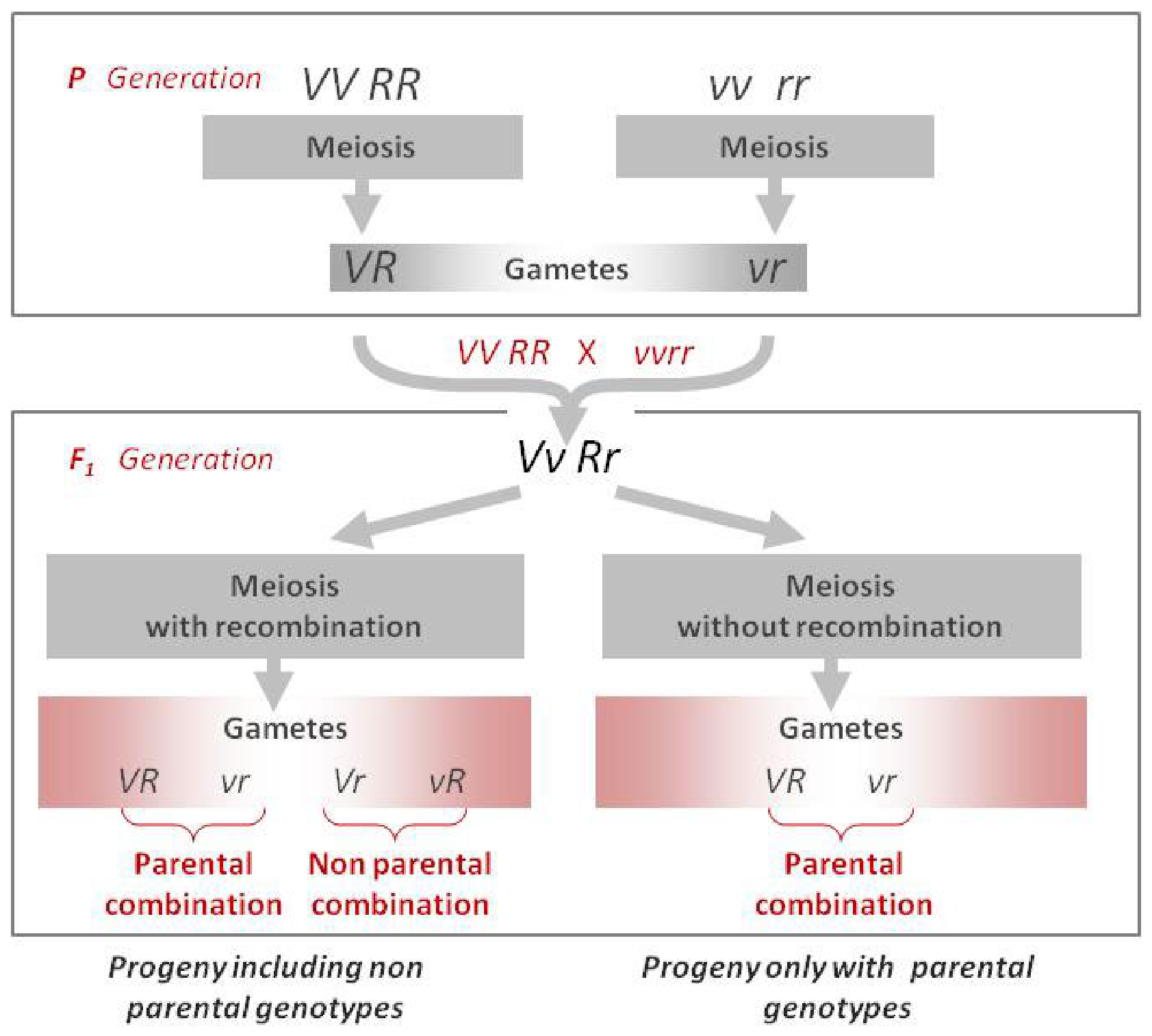
Initially, Morgan generated a dihybrid by crossing a recessive homozygote (vvrr) with a dominant homozygote (VV RR) in both genes. As a result, the F1 dihybrid offspring was expected to be heterozygous for both loci (Vv Rr). Subsequently, females from the F1 generation were testcrossed with males’ homozygous recessive for both genes (vvrr). This testcross ensures that the progeny inherit only recessive alleles from the tester parent, allowing the expressed phenotypes to directly reflect the genotype of the dihybrid female as shown in Figure 1.

The testcross results are shown in

Table 2. The F₂ generation resulting from the testcross between F₁ females and the male tester. The non-parental (recombinant) genotypes are expected to occur at frequencies below 50%, with the remaining proportion corresponding to the parental (non-recombinant) genotypes.

Genotype	Genotype (Shannon’s Representation)	Number of Specimens
VvRr	${\theta }_{\begin{array}{cc}v& r\end{array}}^{\begin{array}{cc}V& R\end{array}}$	1339
vvrr	${\theta }_{\begin{array}{cc}v& r\end{array}}^{\begin{array}{cc}v& r\end{array}}$	1195
Vvrr	${\theta }_{\begin{array}{cc}v& r\end{array}}^{\begin{array}{cc}V& r\end{array}}$	151
vvRr	${\theta }_{\begin{array}{cc}v& r\end{array}}^{\begin{array}{cc}v& R\end{array}}$	154
Sum:		2839

.

The offspring genotypes clearly deviate from the 1:1:1:1 ratio predicted by Mendel’s law of independent assortment. The majority of offspring display parental genotypes, while a smaller proportion exhibit non-parental (recombinant) genotypes. In contrast, complete linkage (100% linkage) would result in only parental gametes being produced. The experimental results indicate that recombination occurs during meiosis, generating a certain proportion of non-parental (recombinant) genotypes. The observed recombination frequency, calculated as ${\displaystyle \frac{151+154}{2839}}\times 100\approx$10.7%, is less than 50%, thereby confirming the presence of genetic linkage. This means recombinant gametes are produced at a lower frequency than parental gametes, which together exceed 50%. The initial Morgan experiments estimated the genetic distance at approximately 10.7% recombination. However, because Morgan’s approach is a stochastic procedure based on finite sample sizes, different experiments or different crosses yield slightly different estimates. Currently, a more precise estimate is available based on the known cytogenetic positions of the two genes: the pr gene (purple eye) is located on chromosome 2 at position 54.5 (Muller element B–2L), and the vg gene (vestigial wings) is located on chromosome 2 at position 67 (Muller element C–2R). Subtracting these two map positions gives 67 − 54.5 = 12.5 map units, corresponding to a recombination frequency of 12.5%. This is the standardized modern estimate and the one used in our validation [24].

An illustration of the use of Shannon’s genetic algebra to compute the frequency of the expected offspring frequencies for the above example is presented below. The calculation of the expected frequency of the offspring with genotype Vvrr (${\theta }_{v r}^{V r}$), which is a non-parental combination resulting from recombination events, is presented in Shannon notation in Equation (28).

$${\lambda }_{v r}^{v r} x {\mu }_{v r}^{V R}={\theta }_{v r}^{V r}={\displaystyle \frac{1}{2}}\left(p_0{\lambda }_{••}^{v r}+p_1{\lambda }_{•r}^{v •}\right)\left(p_0{\mu }_{••}^{V R}+p_1{\mu }_{•R}^{V •}\right)+{\displaystyle \frac{1}{2}}\left(p_0{\lambda }_{••}^{V R}+p_1{\lambda }_{•R}^{V •}\right)\left(p_0{\mu }_{••}^{v r}+p_1{\mu }_{•r}^{v •}\right)$$

(28)

Consider that one male tester contributes all paternal-lineage gametes, which, regardless of recombination events, will always be ${\lambda }_{••}^{v r}$. On the other hand, the female-lineage gametes have the following genotypes: ${\mu }_{••}^{V R}$, ${\mu }_{••}^{v r}$, ${\mu }_{••}^{V r}$, ${\mu }_{••}^{v R}$. Since the chromosome ${\theta }_{v r}^{••}$ is contributed by the tester male, then the remaining ${\theta }_{••}^{V r}$ is contributed by the female. Additionally, in the Thomas Hunt experiment, the recombination frequency was calculated as 0.107. Since a recombination event involves the exchange of genetic material between two homologous chromosomes, the Shannon probability should be half of this value. To clarify the following example, one should consider that, since the offspring has the genotype ${\theta }_{v r}^{V r}$, then the first term implies the probability that $v,r$ are inherited from λ and $V,r$ from μ, whereas the second term implies the probability that $V,r$ are inherited from λ and $v,r$ from μ.

$$\begin{array}{c}{\theta }_{v r}^{V r}={\displaystyle \frac{1}{2}}\left(p_0{\lambda }_{••}^{v r}+p_1{\lambda }_{•r}^{v •}\right)\left(p_0{\mu }_{••}^{V R}+p_1{\mu }_{•R}^{V •}\right)+{\displaystyle \frac{1}{2}}\left(p_0{\lambda }_{••}^{V R}+p_1{\lambda }_{•R}^{V •}\right)\left(p_0{\mu }_{••}^{v r}+p_1{\mu }_{•r}^{v •}\right)=\\ {\displaystyle \frac{1}{2·2839}}\left(0.893·2839+0.107·2839\right)\left(0.893·2839+0.107·2839\right)+{\displaystyle \frac{1}{2}}\left(0\right)(0)\approx {\displaystyle \frac{1}{2·2839}}\left(1\right)\left(304\right)\approx {\displaystyle \frac{152}{2839}}\end{array}$$

(29)

3.2. Shannon’s Product for Finite Populations

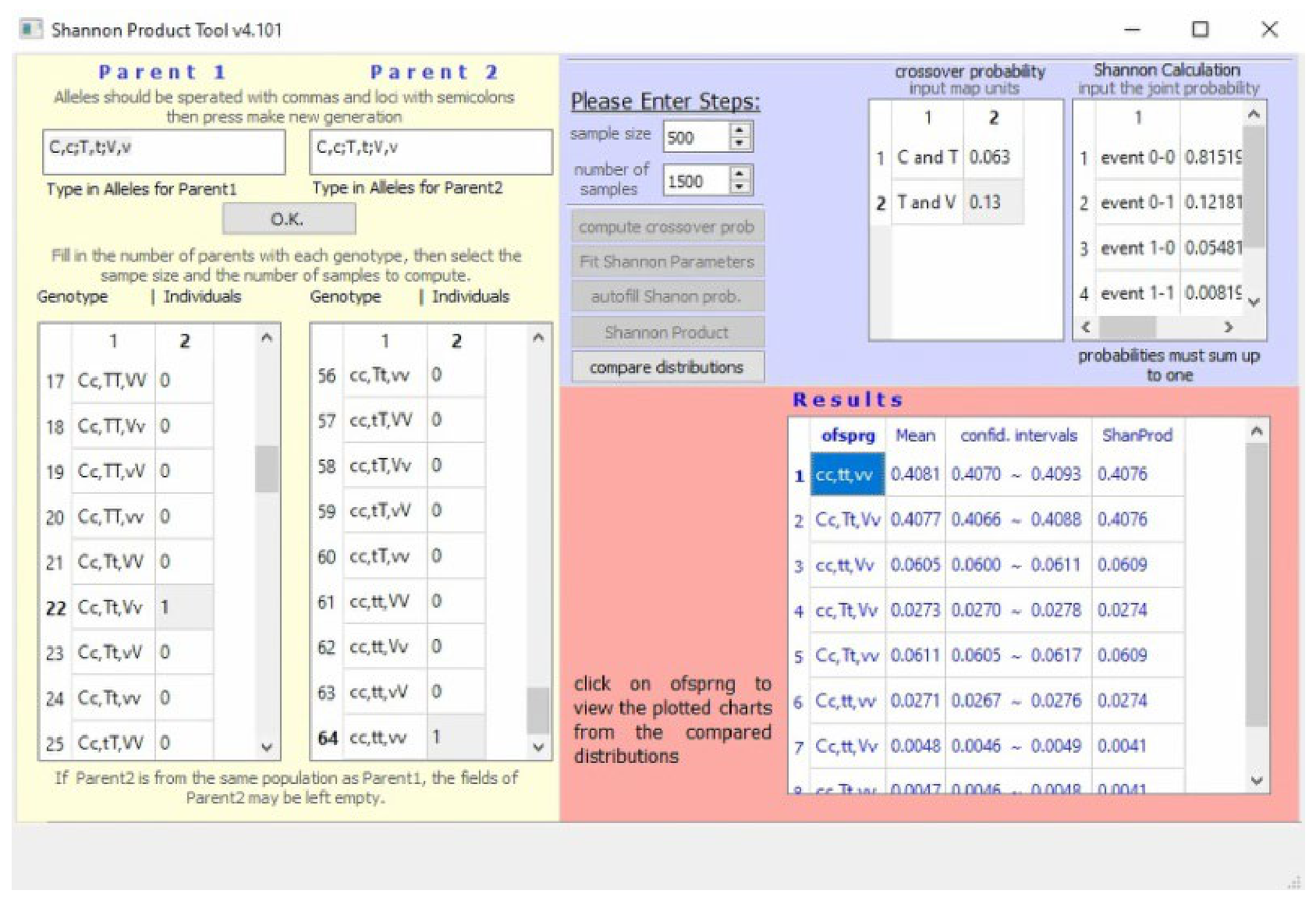
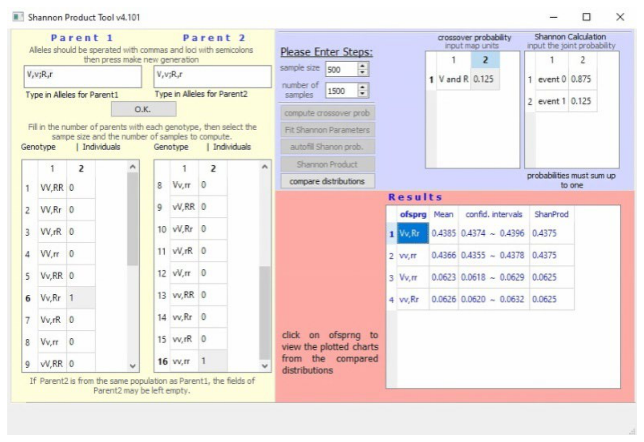
In Appendix A, we present a snapshot of our user-friendly interface, where a user can automatically perform and compare the analytical predictions of Shannon’s algebra with the corresponding stochastic outcomes obtained from a set of finite samples generated under the same assumptions. In the example presented in Figure A1, one parent is assigned the genotype Vv;Rr (a female dihybrid), while the other parent is assigned vv;rr (a tester male). In the blue section, the sample size and the number of samples to be simulated by the application must be entered. Finally, the recombination frequency value is set—in this case, the value 0.125 (as shown in Figure A1), reflecting the currently estimated recombination frequency between these two traits. After computing the Shannon genetic cross-product, the results are summarized in

Table 3. Results obtained after 1500 repetitions of the algorithm on stochastic samples of 500 offspring each, drawn from the same genetic pool, involving three loci.

Offspring	Mean	Stddev	Shannon Prediction
ccttvv	0.4081	0.4070~0.4093	0.4076
CcTtVv	0.4077	0.4066~0.4088	0.4076
ccttVv	0.0605	0.0600~0.0611	0.0609
ccTtVv	0.0273	0.0270~0.0278	0.0274
CcTtvv	0.0611	0.0605~0.0617	0.0609
Ccttvv	0.0271	0.0267~0.0276	0.0274
CcttVv	0.0048	0.0046~0.0049	0.0041
ccTtvv	0.0047	0.0046~0.0048	0.0041

.

The stochastic modeling approach, which generates offspring under the same assumptions as in Shannon’s framework, yields estimates of the imposed recombination frequency (~12.5% in this case) by averaging the stochastic outcomes of recombination relative to the parental genotypes across multiple sample trials.

This imposed recombination frequency (~12.5% in this case), used in the process of generating the offspring samples in our stochastic computational experiment, can be recovered, either as the theoretical limit of an experiment with an infinitely large parental sample or, equivalently, as the limit obtained by averaging over many finite-size parental experiments, as the number of experiments tends to infinity. As in any real-life experiment, each computational experiment yields slightly different genotype frequency outcomes due to the finite size of the samples involved. Repeating the same experiment multiple times allows not only the estimation of the average number of offspring of each genotype but also the construction of histograms showing the frequency of observing each genotype count across an ensemble of repeated computational experiments, with Shannon’s original work providing a method for estimating the expected genotype frequencies as a function of the recombination probability, which can be directly compared with the mean genotypic frequencies obtained over multiple replicates. In Figure A1 and

Table 4. Final results obtained after performing 1500 iterations of the Thomas Hunt Morgan experiment simulation.

Offspring	Mean	Conf. Interv.	Shannon
Vv,Rr	0.4385	0.4374~0.4396	0.4375
vv,rr	0.4366	0.4355~0.4378	0.4375
Vv,rr	0.0623	0.0618~0.0629	0.0625
vv,Rr	0.0626	0.0620~0.0632	0.0625

, we show that, having extended Shannon’s theory to address finite-size samples, we are able to validate both that the observed genotypic frequencies in the offspring population obtained from the stochastic simulation match Shannon’s predictions, and that the estimated genotype distributions, obtained by comparing the analytical solution with histograms of simulated offspring populations, are consistent.

Finally, in Table 4, we present the estimations for the confidence intervals of the finite-size stochastic mating experiments, showing that Shannon’s predictions for the same recombination frequency fall within the confidence interval of the stochastic experiments, as expected.

Table 4 presents the average frequencies for each genotype along with their respective confidence intervals, based on M = 1500 repeated sampling experiments. These values are compared to Shannon’s theoretical probabilities for each offspring genotype.

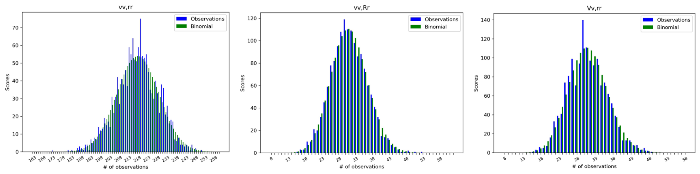
Because the full multinomial distribution of genotype frequencies is difficult to visualize, it is often more practical to plot the distribution of observing a single genotype (relative to all other genotypes combined) using the corresponding binomial distribution. In Figure 2, the binomial distributions-derived form (shown in green) of Equation (30) are plotted alongside the observed histograms for each offspring genotype for the example presented in Table 4. In Equation (30), N denotes the total offspring population, k is the observed count of a specific genotype, and r is the expected probability of that genotype, calculated using Shannon’s genetic product formula.

$$f(k,N,r)=\left(\begin{array}{c}N\\ k\end{array}\right)r^k{\left(1-r\right)}^{N-k}$$

(30)

Equation (30) is also consistent with the numerical estimations of the confidence interval in Table 4. It corresponds to the mean frequency of a genotype across M = 1500 independent simulation experiments, each with sample size N = 500 offspring. The standard error of this mean, evaluated using Equation (30), is $\sqrt{{\displaystyle \frac{r(1-r)}{N\ast M}}}$, which gives 95% confidence intervals in agreement with the numerical estimates reported in Table 4.

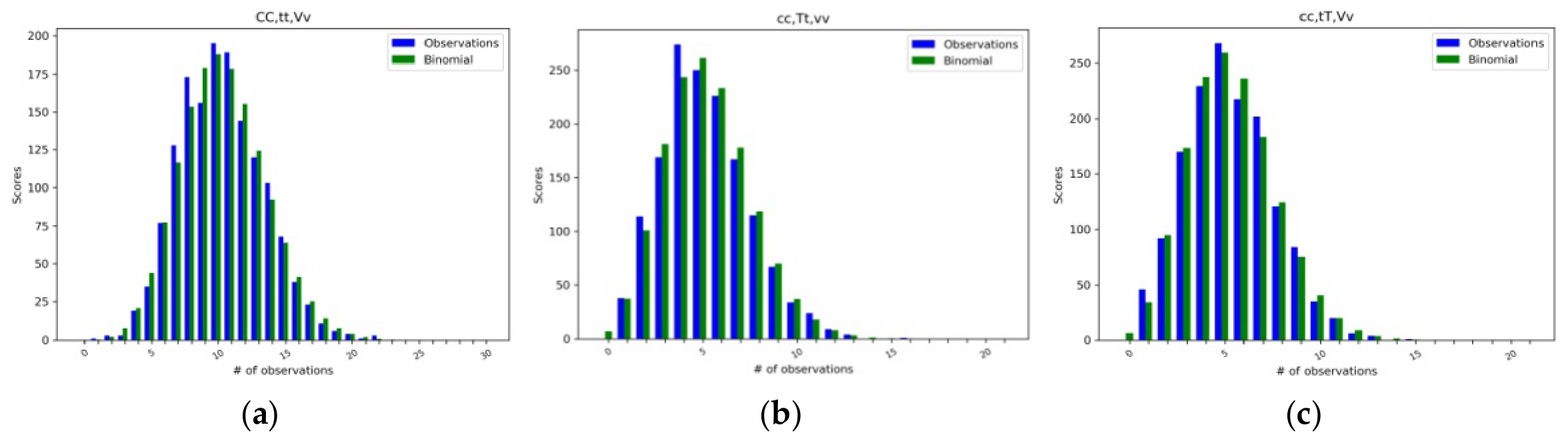
As a second test case, we examined a system using a three-point testcross experiment, with one parent from each genotype. The resulting details are represented in Figure A2 of Appendix A. As in the previous example, we confirmed the theoretical predictions for the average frequencies and the corresponding analytical multinomial distributions by performing a set of finite-size computational experiments and comparing the results with the theoretical estimations.

The input consists of an arbitrary number of parents and offspring selected from a gene pool, with genetic map units distances obtained from flybase.org [24]. The loci A, T and V used in this study correspond to three loci on Muller element A, which is the X chromosome of the Drosophila melanogaster genome—specifically, loci cv, ct and v. The genetic distances between these loci were retrieved from the Drosophila melanogaster observed recombination map and used as input parameters in the algorithm. The genetic distance between C(cv) and T(ct) is 0.063, and between T(ct) and V(v) is 0.13. The results obtained from the proposed algorithm demonstrate that Shannon’s algebra can accurately predict the expected number of offspring for each genotype within a specified parental population. Figure 3 shows a comparison between the theoretical binomial distribution of offspring and their observed genotype distribution, supporting the validity of the algorithm for more complex genetic systems.

3.3. Parental–Offspring Phenotypic Frequency Compatibility Relations

As a practical implementation of Shannon’s algebra within our recent analytical approach to phenotype–genotype mapping, we examine parental–offspring phenotypic compatibility in the simplest possible case: a single genetic locus with two alleles, A (dominant) and a (recessive). These give rise to two phenotypes, A and a, respectively, where phenotypic expression is governed by a dominant–recessive interaction. Specifically, genotypes AA and Aa result in phenotype A, while only genotype aa produces phenotype a, i.e., $\stackrel{̿}{\mathit{{\rm M}}}=\left[\begin{array}{c}\begin{array}{cc}\begin{array}{cc}1& 1\end{array}& \begin{array}{cc}1& 0\end{array}\end{array}\\ \begin{array}{cc}\begin{array}{cc}0& 0\end{array}& \begin{array}{cc}0& 1\end{array}\end{array}\end{array}\right]$. As described in Section 3.3 of the Methods, our aim is to express the analytical relations that connect the phenotypic offspring population to the parental phenotypic trait frequencies. In the simplest example, we consider a fixed phenotypic frequency of 0.7 for A and 0.3 for a (i.e., ${\stackrel{⃑}{\phi }}^{par}={\left[\mathrm{0.7,0.3}\right]}^T$), and identical paternal and maternal genetic populations ${\stackrel{⃑}{\rho }}^{par}={\left[{\lambda }_{\mathrm{A}}^A,{\lambda }_{\mathrm{a}}^A,{\lambda }_{\mathrm{A}}^a,{\lambda }_{\mathrm{a}}^a\right]}^T$. In such a case, as we have shown in our recent work that solving the system of equations presented in Equation (31) yields an analytical expression for ${\stackrel{⃑}{\rho }}^{par}$ as a function of a single auxiliary parameter x, in the form given by Equation (32). This solution can be obtained either analytically or numerically using the Penrose pseudoinverse matrix approach.

$${\stackrel{⃑}{\phi }}^{par}=\stackrel{̿}{\mathit{{\rm M}}}\times {\stackrel{⃑}{\rho }}^{par}\Rightarrow \left[\begin{array}{c}{{\stackrel{⃑}{\phi }}^{par}}_{\mathit{A}}\\ {{\stackrel{⃑}{\phi }}^{par}}_{\mathit{\alpha }}\end{array}\right]=\left[\begin{array}{c}0.7\\ 0.3\end{array}\right]\Rightarrow \left[\begin{array}{c}\begin{array}{cc}\begin{array}{cc}1& 1\end{array}& \begin{array}{cc}1& 0\end{array}\end{array}\\ \begin{array}{cc}\begin{array}{cc}0& 0\end{array}& \begin{array}{cc}0& 1\end{array}\end{array}\end{array}\right]\times \left[\begin{array}{c}{\lambda }_{\mathrm{A}}^A\\ {\lambda }_{\mathrm{a}}^A\\ \begin{array}{c}{\lambda }_{\mathrm{A}}^a\\ {\lambda }_{\mathrm{a}}^a\end{array}\end{array}\right]=\left[\begin{array}{c}0.7\\ 0.3\end{array}\right]$$

(31)

The system in Equation (31) consists of two equations and has three independent unknowns, since ${\lambda }_{•}^{•}=1$. Because the number of equations is less than the number of unknowns, knowledge of the phenotypic frequencies does not determine unique values for the genotypic frequencies. Instead, a set of possible genotypic frequencies is consistent with each phenotypic frequency vector ${\stackrel{⃑}{\phi }}^{par}$. We show that all genotypic frequencies consistent with the given phenotypic frequency are expressed in the form of Equation (32), as a function of an auxiliary variable x:

$$\left[\begin{array}{c}{\lambda }_{\mathrm{A}}^A\\ {\lambda }_{\mathrm{a}}^A\\ \begin{array}{c}{\lambda }_{\mathrm{A}}^a\\ {\lambda }_{\mathrm{a}}^a\end{array}\end{array}\right]=\left[\begin{array}{c}0.816 x+0.233\\ 0.233-0.408 x\\ \begin{array}{c}0.233-0.408 x\\ 0.3\end{array}\end{array}\right]$$

(32)

Equation (32) implies that any parental sample with ${\stackrel{⃑}{\phi }}^{par}={\left[\mathrm{0.7,0.3}\right]}^T$ will have genotypic frequencies ${\stackrel{⃑}{\rho }}^{par}={\left[{\lambda }_{\mathrm{A}}^A,{\lambda }_{\mathrm{a}}^A,{\lambda }_{\mathrm{A}}^a,{\lambda }_{\mathrm{a}}^a\right]}^T$ corresponding to a specific value of the auxiliary variable x. Genotypic frequencies that cannot be expressed for any value of x are not consistent with the phenotypic information and the dominance model imposed through $\stackrel{̿}{\mathit{{\rm M}}}$.

These genotypic frequencies can then be used to compute the haplotype allele frequencies via the step ${\stackrel{⃑}{\rho }}^{par}(\overrightarrow{x},{\stackrel{⃑}{\phi }}^{par})\Rightarrow {\stackrel{⃑}{\lambda }}^{par}(\overrightarrow{x},{\stackrel{⃑}{\phi }}^{par})$, introduced in Section 2.4, which in this example leads to Equation (33):

$$\begin{array}{c}\hfill \stackrel{⃑}{\lambda }=\stackrel{̿}{\mathit{N}}\times \stackrel{⃑}{\rho }=\left[\begin{array}{c}\begin{array}{cc}\begin{array}{cc}1& 0.5\end{array}& \begin{array}{cc}0.5& 0\end{array}\end{array}\\ \begin{array}{cc}\begin{array}{cc}0& 0.5\end{array}& \begin{array}{cc}0.5& 1\end{array}\end{array}\end{array}\right]\left[\begin{array}{c}0.816 x+0.233\\ 0.233-0.408 x\\ \begin{array}{c}0.233-0.408 x\\ 0.3\end{array}\end{array}\right]\\ \hfill \Rightarrow \left[\begin{array}{c}{\lambda }_{•}^A\\ {\lambda }_{•}^a\end{array}\right]=\left[\begin{array}{c}\begin{array}{cc}\begin{array}{cc}1& 0.5\end{array}& \begin{array}{cc}0.5& 0\end{array}\end{array}\\ \begin{array}{cc}\begin{array}{cc}0& 0.5\end{array}& \begin{array}{cc}0.5& 1\end{array}\end{array}\end{array}\right]\left[\begin{array}{c}0.816 x+0.233\\ 0.233-0.408 x\\ \begin{array}{c}0.233-0.408 x\\ 0.3\end{array}\end{array}\right]\Rightarrow \left[\begin{array}{c}{\stackrel{⃑}{\lambda }}_A\\ {\stackrel{⃑}{\lambda }}_{\alpha }\end{array}\right]=\left[\begin{array}{c}0.408x + 0.466\\ 0.533 - 0.408x\end{array}\right]\end{array}$$

(33)

The next step, denoted as ${\stackrel{⃑}{\lambda }}^{par}(\overrightarrow{x},{\stackrel{⃑}{\phi }}^{par})\Rightarrow {\stackrel{⃑}{\rho }}^{offs}(\overrightarrow{x},{\stackrel{⃑}{\phi }}^{par},\overrightarrow{p})$, involves expressing the offspring genotypic frequencies ${\stackrel{⃑}{\rho }}^{offs}$ from the parental allele frequencies ${\stackrel{⃑}{\lambda }}^{par}$ using Shannon’s algebra, as shown in Equation (34) for this example:

$${\stackrel{⃑}{\rho }}^{offs}=\left[\begin{array}{c}{\left({\lambda }_{•}^A\right)}^2\\ {\lambda }_{•}^A{\lambda }_{•}^a\\ \begin{array}{c}{\lambda }_{•}^a{\lambda }_{•}^A\\ {\left({\lambda }_{•}^a\right)}^2\end{array}\end{array}\right]$$

(34)

The final step relates the offspring phenotypic and genotypic frequencies via ${\stackrel{⃑}{\phi }}^{offs}=\stackrel{̿}{\mathit{{\rm M}}}\times {\stackrel{⃑}{\rho }}^{offs}$, resulting in an analytical expression for the offspring phenotypic frequencies consistent with the parental phenotypic frequencies in Equation (31). Equation (35) expresses, as a function of the auxiliary parameter x, the expected offspring phenotypic frequencies compatible with the parental frequencies and the genotype–phenotype map defined by $\stackrel{̿}{\mathit{{\rm M}}}$.

In the case of 100% penetrance, each parental sample corresponds to a single value of x and therefore to a unique average offspring phenotypic frequency ${\stackrel{⃑}{\phi }}^{offs}$, whereas different parental samples correspond to different values of x. For finite samples, one may wish to go beyond the average offspring phenotypic frequency ${\stackrel{⃑}{\phi }}^{offs}$ and construct a distribution over possible offspring phenotypic frequencies, following the approach described in Section 3.2 for expressing the probability density of the possible genotypic frequencies ${\stackrel{⃑}{\rho }}^{offs}$.

In more complex genotype–phenotype mappings involving multiple loci, additional auxiliary parameters may be required to connect phenotypic and genotypic frequencies. In such cases, the resulting analytical expressions depend on both the auxiliary variables and the recombination parameters governing inheritance. Consequently, the framework establishes a direct link between observable phenotypic frequencies and recombination processes, enabling, in principle, the inference of recombination parameters from phenotypic data alone.

$${\stackrel{⃑}{\phi }}^{offs}=\stackrel{̿}{\mathit{{\rm M}}}\times {\stackrel{⃑}{\rho }}^{offs}=\left[\begin{array}{c}\begin{array}{cc}\begin{array}{cc}1& 1\end{array}& \begin{array}{cc}1& 0\end{array}\end{array}\\ \begin{array}{cc}\begin{array}{cc}0& 0\end{array}& \begin{array}{cc}0& 1\end{array}\end{array}\end{array}\right]\times \left[\begin{array}{c}{\left({\lambda }_{•}^A\right)}^2\\ {\lambda }_{•}^A{\lambda }_{•}^a\\ \begin{array}{c}{\lambda }_{•}^a{\lambda }_{•}^A\\ {\left({\lambda }_{•}^a\right)}^2\end{array}\end{array}\right]=\left[\begin{array}{c}-0.166x^2+0.434x+0.713 \\ 0.166x^2-0.435x+0.284\end{array}\right]$$

(35)

As discussed in our recent work [14], the introduction of auxiliary variables in the proposed phenotype-to-genotype mapping is a manifestation of the one-to-many mapping observed in classical genetics. Because any linear transformation of the auxiliary variable would lead to a valid solution, the range of the domain of the function is always set by the condition that all genotypic (and therefore phenotypic) frequencies must be non-negative.

4. Discussion

In this work, we revisit the pioneering doctoral work of Claude E. Shannon, who developed an algebraic representation of Mendelian inheritance as a mathematical function acting on population allele frequencies. Although mathematical methods are now deeply integrated into modern genetics, contemporary approaches rely predominantly on numerical and computational techniques, enabled by advances in high-throughput experimental technologies and large-scale data analysis. In contrast, Shannon’s original work introduced a largely unexplored algebraic framework for representing genetic information and its transmission across generations. Despite having been developed before the molecular basis of inheritance was understood, Shannon’s framework captures the essential mathematical structure of classical Mendelian inheritance, under the standard assumptions of large diploid populations, random mating, the absence of mutation and natural selection, and discrete generations.

The central contribution of this work is the reinterpretation and extension of Shannon’s genetic algebra along two independent yet complementary directions. First, we develop a finite-size formulation that enables Shannon’s framework to be applied to realistic populations, in which inheritance must be described in terms of frequency distributions rather than idealized infinite limits. This extension provides a direct analytical description of how genetic information propagates across generations under finite sampling conditions. Second, we introduce an analytical genotype–phenotype mapping framework that characterizes the set of genotypic and allelic configurations compatible with observed phenotypic frequencies. This formulation demonstrates that phenotypic information defines a constrained manifold of admissible genetic states that can be parameterized through a set of auxiliary variables. Importantly, this framework enables inference at the level of genotypes and alleles without requiring direct genotyping.

Although each of these developments can be applied independently, their combination provides a powerful analytical framework in which phenotypic constraints can be propagated across generations using Shannon’s algebra. This establishes a direct connection between observable phenotypic data and the underlying space of genetic configurations, offering a new perspective on inference in systems where genetic information is incomplete or inaccessible.

A natural point of comparison for the present framework is with phylogenetic reconstruction methods, which aim to infer ancestral relationships among populations or species based on genetic data. Classical phylogenetic approaches typically reconstruct tree-like structures that represent lineage divergence under the assumption of descent from common ancestors, often relying on sequence-level information or well-defined genotypic states. In contrast, the approach developed here does not seek to reconstruct ancestry explicitly. Instead, it characterizes the space of genotypic configurations that are compatible with observed phenotypic frequencies. While phylogenetic methods generally assume relatively homogeneous or well-defined genetic states within populations (e.g., consensus sequences or dominant haplotypes), our framework accommodates arbitrary parental populations described solely in terms at the level of phenotypic distributions, without requiring knowledge of the underlying genotypes. In this sense, the proposed approach operates at a more coarse-grained yet also more flexible level of description. Rather than resolving unique evolutionary histories, it captures the intrinsic degeneracy of genotype–phenotype mappings and characterizes the set of genetic configurations consistent with the observed phenotypic data. This distinction suggests that the two approaches are complementary: phylogenetic methods provide insights into historical relationships and lineage structure, whereas the present framework provides constraints on the range of genetic configurations and evolutionary outcomes that are compatible with the observed phenotypic distributions.

The results presented in Section 2.4 and Section 3.3 establish a direct analytical bridge between genotype–phenotype mapping and Shannon’s algebra, extending the latter from a descriptive framework for genetic inheritance into a predictive tool for the propagation of phenotypic distributions across generations. By expressing the space of genotypic configurations compatible with observed phenotypic frequencies in terms of auxiliary variables, we obtain a structured representation of the intrinsic degeneracy of the genotype–phenotype relationship. This formulation enables phenotypic inheritance to be viewed as a constrained propagation problem, in which parental phenotypic information defines a manifold of admissible genotypic states that, through recombination, generates a corresponding manifold of offspring phenotypic outcomes. Within this framework, classical deterministic inheritance emerges as a limiting case corresponding to complete penetrance, whereas more general scenarios naturally accommodate variability, uncertainty, and stochastic phenotypic expression. This connection provides a principled basis for extending genotype–phenotype inference beyond single-generation analyses and for interpreting phenotypic observations in terms of underlying genetic constraints that govern hereditary transmission.

5. Conclusions

In this work, we re-examine the basic concepts of Shannon’s genetic algebra and develop two complementary extensions that broaden its applicability to modern problems in population genetics. First, a finite-population version of Shannon’s framework is implemented and tested, extending the application of Shannon’s main results beyond the infinite-population limit. Second, we have combined Shannon’s algebra with an analytical genotype–phenotype mapping framework, enabling the derivation of analytical expressions for offspring phenotypic distributions consistent with a given parental population without the need to estimate the genotypic frequencies of the sample.

Finally, we should stress that the calculations reported in Section 3.3, where phenotypic frequencies are mapped from one generation to the next, are exact only under the assumption of genetic equilibrium, even for phenotypic traits characterized by 100% penetrance. Under 100% penetrance, a phenotypic trait is completely determined by the individual’s genotype, and the initial phenotypic mapping within the parental generations does not introduce any stochasticity itself. On the other hand, the estimation in Section 3.3 implicitly assumes the absence of conditions that typically prevent genotypic frequencies from reaching such a genetic equilibrium.

It should be stressed that genetic equilibrium, otherwise referred to as Hardy–Weinberg equilibrium, is known from the pioneering work of Hardy and Weinberg, and independently “reconfirmed” by Shannon’s work, to act as an attractor in genotype frequency space in the absence of selective mating, mutation, migration, and drift. While Hardy–Weinberg equilibrium describes the physical tendency toward a stationary distribution, Shannon’s original work provides an additional description of the evolution toward such a stationary distribution via the recombination process, that is, the underlying mechanism that leads to the stationary distribution in an infinite, randomly mating population.

At the level described in this work, the algebraic modeling of diploid organisms does not include the modeling of mutations, natural selection, or selective breeding. Although Shannon himself proposed an initial approach for including mutations in his work, a complete model that properly includes mutations, natural selection, selective breeding, and recombination within the same framework remains, to our knowledge, an open problem.

Our Python 3.8.18 implementation provides a practical computational tool for applying Shannon’s genetic algebra to problems in genetic inheritance and trait prediction. We offer this work as a foundation for future extensions that will incorporate stochastic inheritance in hypothesis testing involving multilocus systems, and complex phenotypic analysis in a unified framework. It is our hope that this approach will prove useful to researchers working at the interface of population genetics, statistical inference, and computational biology.

References

1. Shannon, C.E. An Algebra for Theoretical Genetics; MIT: Cambridge, MA, USA, 1940. [Google Scholar]
2. Makałowski, W. The Human Genome Structure and Organization. Acta Biochim. Pol. 2001, 48, 587–598. [Google Scholar] [CrossRef] [Scilit]
3. Salzberg, S.L. Open Questions: How Many Genes Do We Have? BMC Biol. 2018, 16, 94. [Google Scholar] [CrossRef] [Scilit] [PubMed]
4. Palazzo, A.F.; Gregory, T.R. The Case for Junk DNA. PLoS Genet. 2014, 10, e1004351. [Google Scholar] [CrossRef] [Scilit] [PubMed]
5. Mayo, O.A. Century of Hardy-Weinberg Equilibrium. Twin Res. Hum. Genet. 2008, 11, 249–256. [Google Scholar] [CrossRef] [Scilit] [PubMed]
6. Graur, D. Molecular and Genome Evolution; Sinauer: Sinauer, MA, USA, 2015. [Google Scholar]
7. Frawley, L.E.; Orr-Weaver, T.L. Polyploidy. Curr. Biol. CB 2015, 25, R353–R358. [Google Scholar] [CrossRef] [Scilit] [PubMed]
8. Bachtrog, D.; Mank, J.E.; Peichel, C.L.; Kirkpatrick, M.; Otto, S.P.; Ashman, T.-L.; Hahn, M.W.; Kitano, J.; Mayrose, I.; Ming, R.; et al. Sex Determination: Why so Many Ways of Doing It? PLoS Biol. 2014, 12, e1001899. [Google Scholar] [CrossRef] [Scilit] [PubMed]
9. Smigielski, E.M.; Sirotkin, K.; Ward, M.; Sherry, S.T. dbSNP: A Database of Single Nucleotide Polymorphisms. Nucleic Acids Res. 2000, 28, 352–355. [Google Scholar] [CrossRef] [Scilit] [PubMed]
10. Griffiths, A.J.F.; Wessler, S.R.; Carroll, S.B.; Doebley, J. An Introduction to Genetic Analysis; Macmillan Learning: New York, NY, USA, 2015. [Google Scholar]
11. Levy, P.A.; Marion, R. Trisomies. Pediatr. Rev. 2018, 39, 104–106. [Google Scholar] [CrossRef] [Scilit] [PubMed]
12. Ohkura, H. Meiosis: An Overview of Key Differences from Mitosis. Cold Spring Harb. Perspect. Biol. 2015, 7, a015859. [Google Scholar] [CrossRef] [Scilit] [PubMed]
13. Whitby, M.C. Making Crossovers during Meiosis. Biochem. Soc. Trans. 2005, 33, 1451–1455. [Google Scholar] [CrossRef] [Scilit]
14. Diamataris, I.G.; Maroulakou, I.; Boulougouris, G.C. On the Use of Algebra in Genetics: From Phenotype to Genotype. Mathematics 2026, 14, 1987. [Google Scholar] [CrossRef] [Scilit]
15. Kousoulis, G. On Shannon’s Algebra for Theoretical Genetics. Master Thesis, DUTH, Alexandroupolis, Greece, 2015. [Google Scholar]
16. Maurits, N. Matrices. In Math for Scientists: Refreshing the Essentials; Maurits, N., Ćurčić-Blake, B., Eds.; Springer International Publishing: Cham, Switzerland, 2023; pp. 131–164. [Google Scholar]
17. Manning, J.T. Recombination Maintains Equilibrium Frequencies of Common Alleles. Heredity 1982, 49, 253–254. [Google Scholar] [CrossRef] [Scilit]
18. Borecki, I.B.; Province, M.A. Linkage and Association: Basic Concepts. In Advances in Genetics; Academic Press: Cambridge, MA, USA, 2008; Volume 60, pp. 51–74. [Google Scholar]
19. Liu, D.; Ma, C.; Hong, W.; Huang, L.; Liu, M.; Liu, H.; Zeng, H.; Deng, D.; Xin, H.; Song, J.; et al. Construction and Analysis of High-Density Linkage Map Using High-Throughput Sequencing Data. PLoS ONE 2014, 9, e98855. [Google Scholar] [CrossRef] [Scilit] [PubMed]
20. Kim, S.Y.; Lohmueller, K.E.; Albrechtsen, A.; Li, Y.; Korneliussen, T.; Tian, G.; Grarup, N.; Jiang, T.; Andersen, G.; Witte, D.; et al. Estimation of Allele Frequency and Association Mapping Using Next-Generation Sequencing Data. BMC Bioinform. 2011, 12, 231. [Google Scholar] [CrossRef] [Scilit] [PubMed]
21. Morgan, T.H. Sex Limited Inheritance in Drosophila. Science 1910, 32, 120–122. [Google Scholar] [CrossRef] [Scilit] [PubMed]
22. Pulst, S.M. Genetic Linkage Analysis. Arch. Neurol. 1999, 56, 667–672. [Google Scholar] [CrossRef] [Scilit] [PubMed]
23. Dooner, H.K. Genetic Fine Structure from Testcross Progeny Analysis. In The Maize Handbook; Freeling, M., Walbot, V., Eds.; Springer: New York, NY, USA, 1994; pp. 303–306. [Google Scholar]
24. FlyBase Consortium Chromosome Maps, 2026. Available online: https://flybase.org/maps/chromosomes/maps (accessed on 14 May 2026).
Figure 1. Schematic of the experiment conducted by Thomas Hunt Morgan, reproduced via the algorithm.
Mathematics 14 02168 g001
Figure 2. Results for three selected observed genotypes obtained from the two locus testcross experiment. It is clear that Shannon’s product accurately predicts the outcomes for finite populations when compared to the corresponding binomial distribution (shown in green).
Mathematics 14 02168 g002
Figure 3. Comparison between the theoretical (binomial prediction—green) and observed (blue) genotype distributions from the three-locus experiment. The horizontal axis represents the number of times a specific genotype is observed among the offspring, while the vertical axis represents the number of simulation runs in which that genotype count was observed. (a) Offspring with genotype CC,tt,Vv, (b) offspring with genotype cc,Tt,vVv, and (c) offspring with genotype cc,tT,Vv.
Mathematics 14 02168 g003