First Optimal Eighth-Order Families with Multivariable Scalar Weight Functions for Nonlinear Systems and Applications to Fredholm Integral and Semilinear Elliptic Problems

Abstract

This paper presents new optimal eighth-order families with weight functions for solving nonlinear systems, obtained as a generalization of the first optimal eighth-order CTT8 method introduced by Cordero, Torregrosa and Triguero-Navarro. The proposed schemes are constructed by combining a Newton-type predictor with high-order correction steps whose weight functions are suitably chosen to preserve optimal convergence while keeping a low computational cost. To the best of our knowledge, this work introduces the first family of optimal eighth-order methods for nonlinear systems, in the sense of the Cordero–Torregrosa conjecture, developed through a weight-function technique. A complete local convergence analysis is carried out under standard smoothness assumptions, proving eighth-order convergence for nondegenerate solutions. The computational efficiency of the proposed methods is also studied and compared with several existing high-order iterative schemes. Numerical experiments on nonlinear systems of different dimensions confirm the theoretical order of convergence and show the robustness of the new families. In addition, a Fredholm integral equation is solved, followed by a semilinear elliptic Dirichlet problem, further illustrating the reliability and computational performance of the proposed weight-function-based methods.

1. Introduction

The numerical solution of nonlinear systems is a central problem in scientific computing, since many mathematical models arising in engineering, mechanics, fluid dynamics, electromagnetism, and reaction–diffusion theory ultimately require the approximation of roots of nonlinear equations. In practice, such systems frequently appear after the discretization of differential, integro-differential, or variational models. Let

$$F:\mathcal{D}\subseteq {\mathbb{R}}^n\to {\mathbb{R}}^n$$

be a sufficiently smooth mapping. We consider the nonlinear system

$$F\left(x\right)=0.$$

To make this general formulation more explicit, one may think of nonlinear systems in both algebraic and discretized forms. A simple two-dimensional prototype is

$$\left\{\begin{array}{c}{x}_1^2+x_2^2-1=0,\hfill \\ e^{x_1}+x_2-1=0,\hfill \end{array}\right.$$

where polynomial and transcendental nonlinearities are coupled in the same system. More demanding examples arise from classical boundary value models, such as Bratu-type or reaction–diffusion problems,

$$\left\{\begin{array}{cc}-\Delta u=\lambda e^u,\hfill & \mathrm{in}\Omega ,\hfill \\ u=0,\hfill & \mathrm{on}\partial \Omega ,\hfill \end{array}\right.$$

or from nonlinear Fredholm integral equations of the form

$$y\left(t\right)=g\left(t\right)+{\int }_a^{b}K(t,s,y\left(s\right))ds.$$

After finite-difference or quadrature discretization, these models lead to nonlinear algebraic systems whose dimension may be large and whose Jacobian matrices may be dense, sparse, ill-conditioned, or expensive to factorize. Consequently, the main computational difficulties are not limited to the existence of nonlinearities; they also include the cost of Jacobian evaluations, the solution of linear systems at each iteration, sensitivity to starting points, and the need to preserve stability while increasing the convergence order.

Therefore, the construction of iterative methods with a high local order of convergence, controlled computational cost, and reliable numerical stability continues to be an active research topic. Classical references such as Traub’s monograph and the book by Ortega and Rheinboldt provide the foundational framework for the analysis of Newton-type schemes and their variants [1,2].

For nonlinear systems, Newton’s method remains the natural benchmark due to its quadratic local convergence and structural simplicity. This method is given by

$$y^{\left(k\right)}=x^{\left(k\right)}-{\left[F^{\prime }\left(x^{\left(k\right)}\right)\right]}^{-1}F\left(x^{\left(k\right)}\right),k=0,1,2,\dots .$$

(1)

In the vectorial setting, Newton’s scheme is also regarded as the first optimal procedure: it attains order two using one evaluation of the Jacobian matrix and one evaluation of the nonlinear function per iteration. However, increasing the order of convergence without significantly increasing the number of Jacobian evaluations, matrix factorizations, or functional evaluations constitutes a major challenge. This issue is especially relevant in the multidimensional case, where the cost associated with linear algebra operations may dominate the overall performance of the iterative process.

The scalar optimality criterion introduced by Kung and Traub [3] motivates, in the vectorial case, an analogous way of measuring optimality according to the number of Jacobian and function evaluations required per iteration. This vectorial optimality criterion will be formally recalled below in Conjecture [4], and it will be used in this work as the reference framework to assess the optimal character of the proposed methods.

Under this criterion, Newton’s method corresponds to the first optimal case, of order two. The next relevant milestone is the construction of optimal fourth-order procedures with $(k_1,k_2)=(1,2)$, and the subsequent target is the construction of optimal eighth-order procedures with $(k_1,k_2)=(1,3)$.

The development of methods attaining the vectorial optimality bound has been gradual and remains limited. After Newton’s method, the construction of optimal fourth-order procedures with $(k_1,k_2)=(1,2)$ represents the natural intermediate step toward eighth-order schemes with $(k_1,k_2)=(1,3)$. More recently, Cordero, Torregrosa and Triguero-Navarro established the first optimal vectorial eighth-order iterative scheme for solving nonlinear systems, thereby reaching the next level in the Cordero–Torregrosa hierarchy [5].

The literature on high-order iterative methods for nonlinear systems has grown steadily in recent years. Representative contributions include Jarratt-like fourth- and sixth-order methods [6], families of fourth- and sixth-order methods together with efficiency and dynamical analyses [7], techniques for systematically increasing the order of convergence of iterative schemes [8], efficient high-order methods for large-scale nonlinear systems [9], semilocal convergence analyses for eighth-order schemes [10], and related developments for structured nonlinear systems [11]. These works show that the field has evolved from fixed multipoint formulas toward more flexible constructions involving accelerators, free parameters, semilocal theory, and dynamical tools.

A particularly fruitful line of research in this context concerns the design of high-order methods through scalar accelerators, parametric families, and weight-function-based techniques for nonlinear systems. Among these strategies, scalar accelerators constructed from quotients of squared norms, for instance

$${\nu }_k={\displaystyle \frac{{∥F\left(y^{\left(k\right)}\right)∥}_2^2}{{∥F\left(x^{\left(k\right)}\right)∥}_2^2}},$$

where $y^{\left(k\right)}$ is an intermediate approximation generated by Newton’s method, have been shown to increase the convergence order without requiring additional functional evaluations. This idea is also related to recent Traub-type constructions for nonlinear systems [12]. However, although the first optimal vectorial eighth-order scheme was recently obtained in [5], the systematic construction of optimal eighth-order families for nonlinear systems by means of weight functions remains, to the best of our knowledge, an open and relevant direction.

Motivated by these considerations, in this work, we introduce a third correction step based on multivariable scalar weight functions, giving rise to new families of optimal eighth-order methods for nonlinear systems. The proposed framework contains, as a particular member, the optimal eighth-order scheme introduced in [5]. The weight functions are designed through suitable Taylor conditions so that the lower-order error terms are canceled and eighth-order convergence is preserved. Since the resulting methods require one Jacobian evaluation and three evaluations of F per iteration, they attain the Cordero–Torregrosa bound. Consequently, the proposed schemes are optimal in the vectorial sense.

The main contribution of this paper is, therefore, twofold. First, it provides a general framework based on weight functions that extends the first optimal vectorial eighth-order scheme from an isolated iterative process to a family of methods. Second, to the best of our knowledge, it presents the first family of optimal eighth-order methods for nonlinear systems, in the sense of the Cordero–Torregrosa conjecture, obtained by means of the weight-function technique. This point distinguishes the present work from previous optimal constructions and connects directly with the role of weight functions as a flexible tool for preserving high-order convergence without increasing the evaluation cost.

The convergence analysis combines Taylor expansions of the nonlinear operator and its Fréchet derivative with expansions of the inverse Jacobian and of the scalar accelerators involved in the correction terms. As a result, explicit sufficient conditions on the weight functions are derived to guarantee eighth-order convergence for nondegenerate solutions. In addition, the computational efficiency of the proposed families is analyzed and compared with that of several existing high-order iterative schemes.

Beyond their theoretical interest, the proposed schemes are relevant for applications requiring highly accurate solutions of nonlinear algebraic systems. In particular, nonlinear systems arising from quadrature discretizations of Fredholm integral equations and from finite-difference discretizations of semilinear elliptic boundary value problems provide natural and meaningful testing environments since they combine nonlinearity, a dense or sparse algebraic structure, and practical computational demands.

The remainder of the paper is organized as follows. In Section 2, we introduce the notation and preliminary expansions required for the convergence analysis. Section 3 is devoted to the construction of the proposed family with weight functions and to the derivation of sufficient conditions on the weight functions that guarantee optimal eighth-order convergence. In Section 4, we present the computational efficiency analysis and numerical experiments on several nonlinear systems, including a nonlinear Fredholm integral equation. Section 5 deals with the application of the proposed methods to nonlinear systems arising from the finite-difference discretization of a two-dimensional semilinear elliptic Dirichlet problem.

2. Preliminary Concepts

Let $F:\mathcal{D}\subseteq {\mathbb{R}}^n\to {\mathbb{R}}^n$ be a sufficiently smooth nonlinear operator defined on an open convex domain, $\mathcal{D}$. Throughout this work, we assume that the nonlinear system

$$F\left(x\right)=0$$

has a solution $\xi \in \mathcal{D}$, such that $F^{\prime }\left(\xi \right)$ is nonsingular. In this case, $\xi$ is referred to as a nondegenerate solution of the nonlinear system. All derivatives required in the subsequent local analysis are assumed to exist and to be continuous in a neighborhood of $\xi$.

For the convergence analysis, we use the standard multilinear notation for higher-order Fréchet derivatives. For $m\ge 1$, the m-th derivative of F at x is regarded as the m-linear mapping

$$\begin{array}{cc}\hfill F^{\left(m\right)}\left(x\right):\underset{m\mathrm{times}}{\underbrace{{\mathbb{R}}^n\times \cdots \times {\mathbb{R}}^n}}& ⟶{\mathbb{R}}^n,\hfill \\ \hfill F^{\left(m\right)}\left(x\right)& \in {\mathcal{L}}_m({\mathbb{R}}^n;{\mathbb{R}}^n).\hfill \end{array}$$

(2)

For ${\omega }_1,\dots ,{\omega }_m\in {\mathbb{R}}^n$, we write

$$F^{\left(m\right)}\left(x\right)({\omega }_1,\dots ,{\omega }_m)=F^{\left(m\right)}\left(x\right){\omega }_1\cdots {\omega }_m,$$

(3)

and, in the repeated-argument case,

$$F^{\left(m\right)}\left(x\right){\omega }^m:=F^{\left(m\right)}\left(x\right)(\omega ,\dots ,\omega ).$$

(4)

If one of the arguments is itself a higher-order derivative term, we use the compact convention

$$\begin{array}{cc}\hfill & F^{\left(m\right)}\left(x\right){\omega }^{m-1}\left(F^{\left(p\right)}\left(x\right){\omega }^p\right):=F^{\left(m\right)}\left(x\right)\left(\underset{m-1}{\underbrace{\omega ,\dots ,\omega }},F^{\left(p\right)}\left(x\right){\omega }^p\right).\hfill \end{array}$$

(5)

Let $x=\xi +\eta$, where $\eta$ is sufficiently small. Since $F^{\prime }\left(\xi \right)$ is invertible, the Taylor expansion of F around $\xi$ can be written as

$$\begin{array}{c}\hfill F(\xi +\eta )=F^{\prime }\left(\xi \right)\left[\eta +C_2{\eta }^2+C_3{\eta }^3+C_4{\eta }^4\right]+\mathcal{O}\left({\eta }^5\right),\end{array}$$

(6)

where

$$C_j={\displaystyle \frac{1}{j!}}{\left[F^{\prime }\left(\xi \right)\right]}^{-1}{F}^{\left(j\right)}\left(\xi \right),j\ge 2,$$

(7)

and $C_j$ is regarded as a j-linear operator from ${\left({\mathbb{R}}^n\right)}^j$ into ${\mathbb{R}}^n$.

Here and throughout the paper, expressions involving the operators $C_j$ are understood according to the multilinear notation introduced above.

The corresponding expansion of the Jacobian is

$$\begin{array}{c}\hfill F^{\prime }(\xi +\eta )=F^{\prime }\left(\xi \right)\left[I+2C_2\eta +3C_3{\eta }^2+4C_4{\eta }^3\right]+\mathcal{O}\left({\eta }^4\right).\end{array}$$

(8)

Consequently, the inverse Jacobian admits the Neumann-type expansion

$$\begin{array}{cc}\hfill {\left[F^{\prime }(\xi +\eta )\right]}^{-1}=& [I-2C_2\eta +\left(4C_2^2-3C_3\right){\eta }^2\hfill \\ \hfill +& \left(-8C_2^3+6C_3{C}_2+6C_2{C}_3-4C_4\right){\eta }^3]{\left[F^{\prime }\left(\xi \right)\right]}^{-1}+\mathcal{O}\left({\eta }^4\right).\hfill \end{array}$$

(9)

For an iterative sequence, $\left\{x^{\left(k\right)}\right\}$, converging to $\xi$, the local error is denoted by

$$e^{\left(k\right)}=x^{\left(k\right)}-\xi .$$

Definition 1

([13]). The sequence $\left\{x^{\left(k\right)}\right\}$ is said to converge locally to ξ with order $p\ge 1$ if there exists a nonzero p-linear operator $\mathcal{T}$, such that

$$e^{(k+1)}=\mathcal{T}{e}^{{\left(k\right)}^p}+\mathcal{O}\left(e^{{\left(k\right)}^{p+1}}\right).$$

(10)

The operator $\mathcal{T}$ determines the leading term of the local error equation.

In the numerical section, the observed convergence order is estimated by means of the approximated computational order of convergence.

Conjecture 1

(Cordero–Torregrosa [4]). Let $F\left(x\right)=0$ be a nonlinear system, and consider an iterative procedure without memory designed to approximate its solutions. Suppose that, at each iteration, the scheme requires $k_1$ evaluations of the Jacobian matrix $F^{\prime }\left(x\right)$ and $k_2$ evaluations of the map $F\left(x\right)$, where $k_1\le k_2$. Then, the attainable local order of convergence p is bounded by

$$p\le 2^{k_1+k_2-1}.$$

The method is said to be optimal precisely when this bound is attained, i.e., when

$$p=2^{k_1+k_2-1}.$$

Definition 2

([14]). The approximated computational order of convergence (ACOC) is defined as

$$p\approx ACOC={\displaystyle \frac{ln\left(∥x^{(k+1)}-x^{\left(k\right)}∥/∥x^{\left(k\right)}-x^{(k-1)}∥\right)}{ln\left(∥x^{\left(k\right)}-x^{(k-1)}∥/∥x^{(k-1)}-x^{(k-2)}∥\right)}},$$

(11)

Finally, since the proposed methods are constructed by weight-function correction steps, we specify the meaning of a weight function in the present framework.

A weight function is an auxiliary scalar-, vector-, or matrix-valued mapping introduced into an iterative scheme to modify one or more correction terms. Its role is to impose suitable cancellations in the local error equation, thereby increasing the convergence order while preserving, as far as possible, the computational efficiency of the method.

3. Eighth-Order Family with Weight Functions and Convergence Analysis

In this section, we introduce the proposed weight-function family of optimal eighth-order methods for solving nonlinear systems. The construction starts from a Newton predictor and a second correction step driven by the scalar accelerator ${\nu }_k$. A third weighted correction is then incorporated through suitable weight functions. The objective is to obtain a broad family of methods preserving eighth-order convergence while containing the original CTT8 scheme as a particular case.

3.1. Local Convergence Theorem

Theorem 1.

Let $F:\mathcal{D}\subseteq {\mathbb{R}}^n\to {\mathbb{R}}^n$ be a sufficiently differentiable nonlinear mapping in a neighborhood of a nondegenerate solution $\xi \in \mathcal{D}$ of the nonlinear system $F\left(x\right)=0$, with $F^{\prime }\left(\xi \right)$ being nonsingular. Consider the iterative family

$$\left\{\begin{array}{cc}\hfill y^{\left(k\right)}& =x^{\left(k\right)}-{\left[F^{\prime }\left(x^{\left(k\right)}\right)\right]}^{-1}F\left(x^{\left(k\right)}\right),\hfill \\ \hfill z^{\left(k\right)}& =y^{\left(k\right)}-{\left[F^{\prime }\left(x^{\left(k\right)}\right)\right]}^{-1}\left((1+{\nu }_k)F\left(y^{\left(k\right)}\right)+2{\nu }_{k}F\left(x^{\left(k\right)}\right)\right),\hfill \\ \hfill x^{(k+1)}& =z^{\left(k\right)}-{\left[F^{\prime }\left(x^{\left(k\right)}\right)\right]}^{-1}\left(H\left({\nu }_k\right)F\left(z^{\left(k\right)}\right)+\mathcal{I}({\alpha }_k,{\delta }_k,{\nu }_k)F\left(x^{\left(k\right)}\right)+G({\alpha }_k,{\beta }_k)F\left(y^{\left(k\right)}\right)\right),\hfill \end{array}\right.$$

(12)

where

$$\begin{array}{cccc}\hfill {\nu }_k& ={\displaystyle \frac{F{\left(y^{\left(k\right)}\right)}^{T}F\left(y^{\left(k\right)}\right)}{F{\left(x^{\left(k\right)}\right)}^{T}F\left(x^{\left(k\right)}\right)}},\hfill & \hfill {\alpha }_k& ={\displaystyle \frac{F{\left(y^{\left(k\right)}\right)}^{T}F\left(z^{\left(k\right)}\right)}{F{\left(x^{\left(k\right)}\right)}^{T}F\left(x^{\left(k\right)}\right)}},\hfill \\ \hfill {\beta }_k& ={\displaystyle \frac{F{\left(z^{\left(k\right)}\right)}^{T}F\left(z^{\left(k\right)}\right)}{F{\left(y^{\left(k\right)}\right)}^{T}F\left(y^{\left(k\right)}\right)}},\hfill & \hfill {\delta }_k& ={\displaystyle \frac{F{\left(z^{\left(k\right)}\right)}^{T}F\left(z^{\left(k\right)}\right)}{F{\left(x^{\left(k\right)}\right)}^{T}F\left(x^{\left(k\right)}\right)}}.\hfill \end{array}$$

(13)

Assume that the weight functions

$$H:\mathbb{R}\to \mathbb{R},\mathcal{I}:{\mathbb{R}}^3\to \mathbb{R},G:{\mathbb{R}}^2\to \mathbb{R},$$

are defined in a neighborhood of the origin and admit the following local expansions:

$$H\left(\nu \right)=h_0+h_1\nu +\mathcal{O}\left({\nu }^2\right),$$

(14)

$$\begin{array}{cc}\hfill \mathcal{I}(\alpha ,\delta ,\nu )=& i_{000}+i_{100}\alpha +i_{010}\delta +i_{001}\nu +{\displaystyle \frac{i_{002}}{2}}{\nu }^2+i_{101}\alpha \nu +{\displaystyle \frac{i_{003}}{6}}{\nu }^3\hfill \\ \hfill & +\mathcal{O}\left({\alpha }^2+\alpha \delta +{\delta }^2+\delta \nu +\alpha {\nu }^2+{\nu }^4\right),\hfill \end{array}$$

(15)

and

$$G(\alpha ,\beta )=g_{00}+g_{10}\alpha +g_{01}\beta +\mathcal{O}\left({\alpha }^2+\alpha \beta +{\beta }^2\right).$$

(16)

where $h_0,h_1,i_{abc},g_{ab}\in \mathbb{R}$ denote the corresponding Taylor coefficients. If the coefficients satisfy

$$\begin{array}{c}{h}_0=1,h_1=0,\\ i_{000}=0,i_{001}=0,i_{002}=0,i_{003}=0,\\ i_{100}=2,i_{010}=4,i_{101}=-2,\\ g_{00}=0,g_{10}=2,g_{01}=1,\end{array}$$

(17)

then the family has local convergence of order at least eight. More precisely,

$$e^{(k+1)}={\Theta }_8{e}^{{\left(k\right)}^8}+\mathcal{O}\left(e^{{\left(k\right)}^9}\right),$$

where ${\Theta }_8$ is the leading eighth-order error coefficient. In the generic case ${\Theta }_8\ne 0$, the order is exactly eight.

Proof. 

Let us denote

$$e^{\left(k\right)}=x^{\left(k\right)}-\xi ,e_y^{\left(k\right)}=y^{\left(k\right)}-\xi ,e_z^{\left(k\right)}=z^{\left(k\right)}-\xi .$$

As in the convergence analysis of the CTT8 scheme in [5], we use the Taylor expansion

$$\begin{array}{cc}\hfill F\left(x^{\left(k\right)}\right)=F^{\prime }\left(\xi \right)(& e^{\left(k\right)}+C_2{e}^{{\left(k\right)}^2}+C_3{e}^{{\left(k\right)}^3}+C_4{e}^{{\left(k\right)}^4}\hfill \\ \hfill & +C_5{e}^{{\left(k\right)}^5}+C_6{e}^{{\left(k\right)}^6}+C_7{e}^{{\left(k\right)}^7})+\mathcal{O}\left(e^{{\left(k\right)}^8}\right),\hfill \end{array}$$

(18)

where

$$C_j={\displaystyle \frac{1}{j!}}{\left[F^{\prime }\left(\xi \right)\right]}^{-1}{F}^{\left(j\right)}\left(\xi \right),j\ge 2.$$

(19)

The corresponding Jacobian expansion is

$$\begin{array}{cc}\hfill F^{\prime }\left(x^{\left(k\right)}\right)=F^{\prime }\left(\xi \right)(& I+2C_2{e}^{\left(k\right)}+3C_3{e}^{{\left(k\right)}^2}+4C_4{e}^{{\left(k\right)}^3}\hfill \\ \hfill & +5C_5{e}^{{\left(k\right)}^4}+6C_6{e}^{{\left(k\right)}^5}+7C_7{e}^{{\left(k\right)}^6})+\mathcal{O}\left(e^{{\left(k\right)}^7}\right).\hfill \end{array}$$

(20)

Therefore,

$$\begin{array}{cc}\hfill {\left[F^{\prime }\left(x^{\left(k\right)}\right)\right]}^{-1}=(& I+D_1{e}^{\left(k\right)}+D_2{e}^{{\left(k\right)}^2}+D_3{e}^{{\left(k\right)}^3}\hfill \\ \hfill & +D_4{e}^{{\left(k\right)}^4}+D_5{e}^{{\left(k\right)}^5}+D_6{e}^{{\left(k\right)}^6}){\left[F^{\prime }\left(\xi \right)\right]}^{-1}+\mathcal{O}\left(e^{{\left(k\right)}^7}\right),\hfill \end{array}$$

(21)

where the coefficients $D_j$ are determined from

$${\left[F^{\prime }\left(x^{\left(k\right)}\right)\right]}^{-1}{F}^{\prime }\left(x^{\left(k\right)}\right)=I.$$

In particular,

$$\begin{array}{cc}\hfill D_1=& -2C_2,\hfill \\ \hfill D_2=& 4C_2^2-3C_3,\hfill \\ \hfill D_3=& -8C_2^3+6C_2{C}_3+6C_3{C}_2-4C_4,\hfill \\ \hfill D_4=& 16C_2^4-12C_2^2{C}_3-12C_2{C}_3{C}_2-12C_3{C}_2^2+8C_2{C}_4+8C_4{C}_2+9C_3^2-5C_5,\hfill \\ \hfill D_5=& -32C_2^5+24C_2^3{C}_3+24C_2^2{C}_3{C}_2+24C_2{C}_3{C}_2^2+24C_3{C}_2^3\hfill \\ \hfill & -16C_2^2{C}_4-16C_2{C}_4{C}_2-16C_4{C}_2^2-18C_2{C}_3^2-18C_3{C}_2{C}_3-18C_3^2{C}_2\hfill \\ \hfill & +10C_2{C}_5+10C_5{C}_2+12C_3{C}_4+12C_4{C}_3-6C_6,\hfill \\ \hfill D_6=& 64C_2^6-48C_2^4{C}_3-48C_2^3{C}_3{C}_2-48C_2^2{C}_3{C}_2^2-48C_2{C}_3{C}_2^3-48C_3{C}_2^4\hfill \\ \hfill & +32C_2^3{C}_4+32C_2^2{C}_4{C}_2+32C_2{C}_4{C}_2^2+32C_4{C}_2^3\hfill \\ \hfill & +36C_2^2{C}_3^2+36C_2{C}_3{C}_2{C}_3+36C_3{C}_2^2{C}_3+36C_2{C}_3^2{C}_2+36C_3{C}_2{C}_3{C}_2\hfill \\ \hfill & +36C_3^2{C}_2^2-20C_2^2{C}_5-20C_2{C}_5{C}_2-20C_5{C}_2^2\hfill \\ \hfill & -24C_2{C}_3{C}_4-24C_3{C}_2{C}_4-24C_2{C}_4{C}_3-24C_4{C}_2{C}_3-24C_3{C}_4{C}_2-24C_4{C}_3{C}_2\hfill \\ \hfill & -27C_3^3+12C_2{C}_6+12C_6{C}_2+15C_3{C}_5+15C_5{C}_3+16C_4^2-7C_7.\hfill \end{array}$$

(22)

From the Newton step, one obtains

$$\begin{array}{cc}\hfill e_y^{\left(k\right)}=& Y_2{e}^{{\left(k\right)}^2}+Y_3{e}^{{\left(k\right)}^3}+Y_4{e}^{{\left(k\right)}^4}+Y_5{e}^{{\left(k\right)}^5}\hfill \\ \hfill & +Y_6{e}^{{\left(k\right)}^6}+Y_7{e}^{{\left(k\right)}^7}+\mathcal{O}\left(e^{{\left(k\right)}^8}\right),\hfill \end{array}$$

(23)

with

$$\begin{array}{cc}\hfill Y_2=& C_2,\hfill \\ \hfill Y_3=& 2C_3-2C_2^2,\hfill \\ \hfill Y_4=& 4C_2^3-4C_2{C}_3-3C_3{C}_2+3C_4,\hfill \\ \hfill Y_5=& -8C_2^4+8C_2^2{C}_3+6C_2{C}_3{C}_2+6C_3{C}_2^2-6C_2{C}_4-4C_4{C}_2\hfill \\ \hfill & -6C_3^2+4C_5,\hfill \\ \hfill Y_6=& 16C_2^5-16C_2^3{C}_3-12C_2^2{C}_3{C}_2-12C_2{C}_3{C}_2^2-12C_3{C}_2^3\hfill \\ \hfill & +12C_2^2{C}_4+8C_2{C}_4{C}_2+8C_4{C}_2^2+12C_2{C}_3^2+12C_3{C}_2{C}_3\hfill \\ \hfill & +9C_3^2{C}_2-8C_2{C}_5-5C_5{C}_2-9C_3{C}_4-8C_4{C}_3+5C_6,\hfill \\ \hfill Y_7=& -32C_2^6+32C_2^4{C}_3+24C_2^3{C}_3{C}_2+24C_2^2{C}_3{C}_2^2+24C_2{C}_3{C}_2^3\hfill \\ \hfill & +24C_3{C}_2^4-24C_2^3{C}_4-16C_2^2{C}_4{C}_2-16C_2{C}_4{C}_2^2-16C_4{C}_2^3\hfill \\ \hfill & -24C_2^2{C}_3^2-24C_2{C}_3{C}_2{C}_3-18C_2{C}_3^2{C}_2-24C_3{C}_2^2{C}_3\hfill \\ \hfill & -18C_3{C}_2{C}_3{C}_2-18C_3^2{C}_2^2+16C_2^2{C}_5+10C_2{C}_5{C}_2+10C_5{C}_2^2\hfill \\ \hfill & +18C_2{C}_3{C}_4+16C_2{C}_4{C}_3+18C_3{C}_2{C}_4+12C_3{C}_4{C}_2\hfill \\ \hfill & +16C_4{C}_2{C}_3+12C_4{C}_3{C}_2+18C_3^3-10C_2{C}_6-6C_6{C}_2\hfill \\ \hfill & -12C_3{C}_5-10C_5{C}_3-12C_4^2+6C_7.\hfill \end{array}$$

(24)

Consequently,

$$\begin{array}{cc}\hfill F\left(y^{\left(k\right)}\right)=F^{\prime }\left(\xi \right)(& {\widehat{Y}}_2{e}^{{\left(k\right)}^2}+{\widehat{Y}}_3{e}^{{\left(k\right)}^3}+{\widehat{Y}}_4{e}^{{\left(k\right)}^4}+{\widehat{Y}}_5{e}^{{\left(k\right)}^5}+{\widehat{Y}}_6{e}^{{\left(k\right)}^6}+{\widehat{Y}}_7{e}^{{\left(k\right)}^7})+\mathcal{O}\left(e^{{\left(k\right)}^8}\right),\hfill \end{array}$$

(25)

where

$$\begin{array}{cc}\hfill {\widehat{Y}}_2=& Y_2,\hfill \\ \hfill {\widehat{Y}}_3=& Y_3,\hfill \\ \hfill {\widehat{Y}}_4=& Y_4+C_2{Y}_2^2,\hfill \\ \hfill {\widehat{Y}}_5=& Y_5+2C_2{Y}_2{Y}_3,\hfill \\ \hfill {\widehat{Y}}_6=& Y_6+C_2\left(2Y_2{Y}_4+Y_3^2\right)+C_3{Y}_2^3,\hfill \\ \hfill {\widehat{Y}}_7=& Y_7+2C_2\left(Y_2{Y}_5+Y_3{Y}_4\right)+3C_3{Y}_2^2{Y}_3.\hfill \end{array}$$

(26)

Here, the products involving $C_j$ are understood in the multilinear sense introduced in the preliminary notation.

Now, we describe the asymptotic behavior of the scalar accelerators. Since $F^{\prime }\left(\xi \right)$ is nonsingular, and

$$e_y^{\left(k\right)}=\mathcal{O}\left(e^{{\left(k\right)}^2}\right),$$

we have

$${\parallel F\left(x^{\left(k\right)}\right)\parallel }_2^2=\mathcal{O}\left(e^{{\left(k\right)}^2}\right),{\parallel F\left(y^{\left(k\right)}\right)\parallel }_2^2=\mathcal{O}\left(e^{{\left(k\right)}^4}\right).$$

Therefore,

$${\nu }_k={\displaystyle \frac{F{\left(y^{\left(k\right)}\right)}^{T}F\left(y^{\left(k\right)}\right)}{F{\left(x^{\left(k\right)}\right)}^{T}F\left(x^{\left(k\right)}\right)}}=\mathcal{O}\left(e^{{\left(k\right)}^2}\right).$$

More precisely, by expanding the scalar numerator and denominator in powers of $e^{\left(k\right)}$, and since the leading scalar coefficient of $\parallel F\left(x^{\left(k\right)}\right){\parallel }_2^2$ is nonzero, the quotient admits the expansion

$${\nu }_k=n_2{e}^{{\left(k\right)}^2}+n_3{e}^{{\left(k\right)}^3}+n_4{e}^{{\left(k\right)}^4}+n_5{e}^{{\left(k\right)}^5}+\mathcal{O}\left(e^{{\left(k\right)}^6}\right),$$

where $n_2,n_3,n_4,n_5$ are coefficients determined by the Taylor coefficients of F. Their explicit expressions are not required for the cancellation argument below; only the existence of this expansion and the order ${\nu }_k=\mathcal{O}\left(e^{{\left(k\right)}^2}\right)$ are used.

The remaining quantities required in the third correction admit the expansion

$$e_z^{\left(k\right)}=Z_4{e}^{{\left(k\right)}^4}+Z_5{e}^{{\left(k\right)}^5}+Z_6{e}^{{\left(k\right)}^6}+Z_7{e}^{{\left(k\right)}^7}+\mathcal{O}\left(e^{{\left(k\right)}^8}\right),$$

(27)

where $Z_4,Z_5,Z_6$, and $Z_7$ are multilinear coefficients obtained from the second correction step. Since $e_z^{\left(k\right)}=\mathcal{O}\left(e^{{\left(k\right)}^4}\right)$, the nonlinear terms in the Taylor expansion of $F\left(z^{\left(k\right)}\right)$ start at order eight. Hence,

$$F\left(z^{\left(k\right)}\right)=F^{\prime }\left(\xi \right)\left(Z_4{e}^{{\left(k\right)}^4}+Z_5{e}^{{\left(k\right)}^5}+Z_6{e}^{{\left(k\right)}^6}+Z_7{e}^{{\left(k\right)}^7}\right)+\mathcal{O}\left(e^{{\left(k\right)}^8}\right).$$

(28)

Furthermore,

$$\begin{array}{cc}\hfill {\alpha }_k& =a_4{e}^{{\left(k\right)}^4}+a_5{e}^{{\left(k\right)}^5}+a_6{e}^{{\left(k\right)}^6}+\mathcal{O}\left(e^{{\left(k\right)}^7}\right),\hfill \\ \hfill {\beta }_k& =b_4{e}^{{\left(k\right)}^4}+b_5{e}^{{\left(k\right)}^5}+\mathcal{O}\left(e^{{\left(k\right)}^6}\right),\hfill \\ \hfill {\delta }_k& =d_6{e}^{{\left(k\right)}^6}+\mathcal{O}\left(e^{{\left(k\right)}^7}\right),\hfill \end{array}$$

(29)

where $a_4,a_5,a_6,b_4,b_5,d_6$ are real coefficients obtained from the preceding Taylor expansions. Their explicit expressions are not needed in the cancellation argument; only the orders of ${\alpha }_k$, ${\beta }_k$, and ${\delta }_k$ are required.

The third step can be expressed as

$$e^{(k+1)}=e_z^{\left(k\right)}-{\left[F^{\prime }\left(x^{\left(k\right)}\right)\right]}^{-1}{\Psi }_k,$$

(30)

where

$${\Psi }_k=H\left({\nu }_k\right)F\left(z^{\left(k\right)}\right)+\mathcal{I}({\alpha }_k,{\delta }_k,{\nu }_k)F\left(x^{\left(k\right)}\right)+G({\alpha }_k,{\beta }_k)F\left(y^{\left(k\right)}\right).$$

(31)

Using the expansion of H, we obtain

$$\begin{array}{cc}\hfill H\left({\nu }_k\right)F\left(z^{\left(k\right)}\right)& =F^{\prime }\left(\xi \right)(h_0{Z}_4{e}^{{\left(k\right)}^4}+h_0{Z}_5{e}^{{\left(k\right)}^5}+\left(h_0{Z}_6+h_1{n}_2{Z}_4\right)e^{{\left(k\right)}^6}\hfill \\ \hfill & +\left(h_0{Z}_7+h_1(n_2{Z}_5+n_3{Z}_4)\right)e^{{\left(k\right)}^7})+\mathcal{O}\left(e^{{\left(k\right)}^8}\right).\hfill \end{array}$$

(32)

Similarly, from the local expansion of $\mathcal{I}$ around the origin,

$$\begin{array}{cc}\hfill \mathcal{I}({\alpha }_k,{\delta }_k,{\nu }_k)& =i_{000}+i_{001}{n}_2{e}^{{\left(k\right)}^2}+i_{001}{n}_3{e}^{{\left(k\right)}^3}+\left(i_{100}{a}_4+i_{001}{n}_4+{\displaystyle \frac{i_{002}}{2}}{n}_2^2\right)e^{{\left(k\right)}^4}\hfill \\ \hfill & +\left(i_{100}{a}_5+i_{001}{n}_5+i_{002}{n}_2{n}_3\right)e^{{\left(k\right)}^5}\hfill \\ \hfill & +\left(i_{100}{a}_6+i_{010}{d}_6+i_{101}{a}_4{n}_2+{\displaystyle \frac{i_{002}}{2}}(2n_2{n}_4+n_3^2)+{\displaystyle \frac{i_{003}}{6}}{n}_2^3\right)e^{{\left(k\right)}^6}\hfill \\ \hfill & +\mathcal{O}\left(e^{{\left(k\right)}^7}\right).\hfill \end{array}$$

(33)

For brevity, define

$$\begin{array}{cc}\hfill {\eta }_0=& i_{000},{\eta }_2=i_{001}{n}_2,{\eta }_3=i_{001}{n}_3,\hfill \\ \hfill {\eta }_4=& i_{100}{a}_4+i_{001}{n}_4+{\displaystyle \frac{i_{002}}{2}}{n}_2^2,{\eta }_5=i_{100}{a}_5+i_{001}{n}_5+i_{002}{n}_2{n}_3,\hfill \\ \hfill {\eta }_6=& i_{100}{a}_6+i_{010}{d}_6+i_{101}{a}_4{n}_2+{\displaystyle \frac{i_{002}}{2}}\left(2n_2{n}_4+n_3^2\right)+{\displaystyle \frac{i_{003}}{6}}{n}_2^3.\hfill \end{array}$$

(34)

Thus,

$$\begin{array}{cc}\hfill \mathcal{I}({\alpha }_k,{\delta }_k,{\nu }_k)F\left(x^{\left(k\right)}\right)& =F^{\prime }\left(\xi \right)({\eta }_0{e}^{\left(k\right)}+{\eta }_0{C}_2{e}^{{\left(k\right)}^2}+({\eta }_0{C}_3+{\eta }_2)e^{{\left(k\right)}^3}\hfill \\ \hfill & +({\eta }_0{C}_4+{\eta }_2{C}_2+{\eta }_3)e^{{\left(k\right)}^4}\hfill \\ \hfill & +({\eta }_0{C}_5+{\eta }_2{C}_3+{\eta }_3{C}_2+{\eta }_4)e^{{\left(k\right)}^5}\hfill \\ \hfill & +({\eta }_0{C}_6+{\eta }_2{C}_4+{\eta }_3{C}_3+{\eta }_4{C}_2+{\eta }_5)e^{{\left(k\right)}^6}\hfill \\ \hfill & +({\eta }_0{C}_7+{\eta }_2{C}_5+{\eta }_3{C}_4+{\eta }_4{C}_3+{\eta }_5{C}_2+{\eta }_6)e^{{\left(k\right)}^7})\hfill \\ \hfill & +\mathcal{O}\left(e^{{\left(k\right)}^8}\right).\hfill \end{array}$$

(35)

On the other hand,

$$G({\alpha }_k,{\beta }_k)=g_{00}+(g_{10}{a}_4+g_{01}{b}_4)e^{{\left(k\right)}^4}+(g_{10}{a}_5+g_{01}{b}_5)e^{{\left(k\right)}^5}+\mathcal{O}\left(e^{{\left(k\right)}^6}\right).$$

Let us denote

$${\zeta }_0=g_{00},{\zeta }_4=g_{10}{a}_4+g_{01}{b}_4,{\zeta }_5=g_{10}{a}_5+g_{01}{b}_5.$$

Then,

$$\begin{array}{cc}\hfill G({\alpha }_k,{\beta }_k)F\left(y^{\left(k\right)}\right)& =F^{\prime }\left(\xi \right)({\zeta }_0{\widehat{Y}}_2{e}^{{\left(k\right)}^2}+{\zeta }_0{\widehat{Y}}_3{e}^{{\left(k\right)}^3}+{\zeta }_0{\widehat{Y}}_4{e}^{{\left(k\right)}^4}\hfill \\ \hfill & +{\zeta }_0{\widehat{Y}}_5{e}^{{\left(k\right)}^5}+({\zeta }_0{\widehat{Y}}_6+{\zeta }_4{\widehat{Y}}_2)e^{{\left(k\right)}^6}\hfill \\ \hfill & +({\zeta }_0{\widehat{Y}}_7+{\zeta }_4{\widehat{Y}}_3+{\zeta }_5{\widehat{Y}}_2)e^{{\left(k\right)}^7})+\mathcal{O}\left(e^{{\left(k\right)}^8}\right).\hfill \end{array}$$

(36)

Adding (32), (35), and (36), we get

$${\Psi }_k=F^{\prime }\left(\xi \right)\left({\Lambda }_1{e}^{\left(k\right)}+{\Lambda }_2{e}^{{\left(k\right)}^2}+\dots +{\Lambda }_7{e}^{{\left(k\right)}^7}\right)+\mathcal{O}\left(e^{{\left(k\right)}^8}\right),$$

(37)

where

$$\begin{array}{cc}\hfill {\Lambda }_1=& {\eta }_0,\hfill \\ \hfill {\Lambda }_2=& {\eta }_0{C}_2+{\zeta }_0{\widehat{Y}}_2,\hfill \\ \hfill {\Lambda }_3=& {\eta }_0{C}_3+{\eta }_2+{\zeta }_0{\widehat{Y}}_3,\hfill \\ \hfill {\Lambda }_4=& h_0{Z}_4+{\eta }_0{C}_4+{\eta }_2{C}_2+{\eta }_3+{\zeta }_0{\widehat{Y}}_4,\hfill \\ \hfill {\Lambda }_5=& h_0{Z}_5+{\eta }_0{C}_5+{\eta }_2{C}_3+{\eta }_3{C}_2+{\eta }_4+{\zeta }_0{\widehat{Y}}_5,\hfill \\ \hfill {\Lambda }_6=& h_0{Z}_6+h_1{n}_2{Z}_4+{\eta }_0{C}_6+{\eta }_2{C}_4+{\eta }_3{C}_3+{\eta }_4{C}_2+{\eta }_5\hfill \\ \hfill & +{\zeta }_0{\widehat{Y}}_6+{\zeta }_4{\widehat{Y}}_2,\hfill \\ \hfill {\Lambda }_7=& h_0{Z}_7+h_1(n_2{Z}_5+n_3{Z}_4)+{\eta }_0{C}_7+{\eta }_2{C}_5+{\eta }_3{C}_4+{\eta }_4{C}_3\hfill \\ \hfill & +{\eta }_5{C}_2+{\eta }_6+{\zeta }_0{\widehat{Y}}_7+{\zeta }_4{\widehat{Y}}_3+{\zeta }_5{\widehat{Y}}_2.\hfill \end{array}$$

(38)

Substituting (21) and (37) into (30), we obtain

$$e^{(k+1)}=M_1{e}^{\left(k\right)}+M_2{e}^{{\left(k\right)}^2}+\cdots +M_7{e}^{{\left(k\right)}^7}+\mathcal{O}\left(e^{{\left(k\right)}^8}\right),$$

where

$$\begin{array}{cc}\hfill M_1& =-{\Lambda }_1,\hfill \\ \hfill M_2& =-({\Lambda }_2+D_1{\Lambda }_1),\hfill \\ \hfill M_3& =-({\Lambda }_3+D_1{\Lambda }_2+D_2{\Lambda }_1),\hfill \\ \hfill M_4& =Z_4-({\Lambda }_4+D_1{\Lambda }_3+D_2{\Lambda }_2+D_3{\Lambda }_1),\hfill \\ \hfill M_5& =Z_5-({\Lambda }_5+D_1{\Lambda }_4+D_2{\Lambda }_3+D_3{\Lambda }_2+D_4{\Lambda }_1),\hfill \\ \hfill M_6& =Z_6-({\Lambda }_6+D_1{\Lambda }_5+D_2{\Lambda }_4+D_3{\Lambda }_3+D_4{\Lambda }_2+D_5{\Lambda }_1),\hfill \\ \hfill M_7& =Z_7-({\Lambda }_7+D_1{\Lambda }_6+D_2{\Lambda }_5+D_3{\Lambda }_4+D_4{\Lambda }_3+D_5{\Lambda }_2+D_6{\Lambda }_1).\hfill \end{array}$$

(39)

The required cancellation conditions are obtained successively. Since

$$M_1=-i_{000},$$

the first coefficient vanishes by taking

$$i_{000}=0.$$

Under this condition, we have

$$M_2=-g_{00}{Y}_2,$$

and hence, $M_2=0$ is ensured by imposing

$$g_{00}=0.$$

With $i_{000}=g_{00}=0$, we obtain

$$M_3=-i_{001}{n}_2.$$

Therefore, $M_3=0$ is obtained by taking

$$i_{001}=0.$$

Using the preceding conditions, the fourth-order coefficient reduces to

$$M_4=(1-h_0)Z_4.$$

Thus, $M_4=0$ is ensured by imposing

$$h_0=1.$$

Next, under

$$i_{000}=g_{00}=i_{001}=0,h_0=1,$$

one has

$$M_5=-\left((i_{100}-2)a_4+{\displaystyle \frac{i_{002}}{2}}{n}_2^2\right).$$

Consequently, $M_5=0$ is obtained by taking

$$i_{100}=2,i_{002}=0.$$

When, in addition, $i_{100}=2$ and $i_{002}=0$ are assumed, the sixth-order coefficient reduces to

$$M_6=-\left(h_1{n}_2{Z}_4+(g_{10}-2)a_4{Y}_2+(g_{01}-1)b_4{Y}_2\right).$$

Therefore, $M_6=0$ is ensured by imposing

$$h_1=0,g_{10}=2,g_{01}=1.$$

Finally, under all previous conditions, the seventh-order coefficient becomes

$$M_7=-\left((i_{010}-4)d_6+(i_{101}+2)a_4{n}_2+{\displaystyle \frac{i_{003}}{6}}{n}_2^3\right).$$

Hence, $M_7=0$ is obtained by taking

$$i_{010}=4,i_{101}=-2,i_{003}=0.$$

Collecting these conditions, we have

$$M_1=M_2=M_3=M_4=M_5=M_6=M_7=0.$$

Therefore,

$$e^{(k+1)}={\Theta }_8{e}^{{\left(k\right)}^8}+\mathcal{O}\left(e^{{\left(k\right)}^9}\right),$$

where ${\Theta }_8$ is the leading eighth-order error coefficient. Hence, the proposed family has a local convergence of the order of at least eight.    □

Remark 1.

The coefficient conditions in (17) can also be expressed in terms of the derivatives of the weight functions at the origin. In particular,

$$h_0=H\left(0\right),h_1=H^{\prime }\left(0\right),$$

while the coefficients $i_{abc}$ and $g_{ab}$ correspond to the Taylor coefficients of $\mathcal{I}$ and G, respectively. Thus, the conditions

$$i_{002}=0,i_{003}=0$$

are equivalent to

$${\mathcal{I}}_{\nu \nu }(0,0,0)=0,{\mathcal{I}}_{\nu \nu \nu }(0,0,0)=0.$$

Therefore, if one restricts the admissible class of weight functions $\mathcal{I}$ by excluding pure terms in ${\nu }^2$ and ${\nu }^3$, these two conditions are automatically satisfied. In this reduced formulation, the practical conditions become

$$h_0=1,h_1=0,$$

$$i_{000}=0,i_{001}=0,i_{100}=2,i_{010}=4,i_{101}=-2,$$

and

$$g_{00}=0,g_{10}=2,g_{01}=1.$$

This reduced formulation is the one most commonly used in practical implementations of the family.

3.2. Admissible Weight Functions

Corollary 1.

Assume the hypotheses of Theorem 1. Consider the class of weight functions satisfying

$$H\left(\nu \right)=1+\mathcal{O}\left({\nu }^2\right),$$

(40)

$$\mathcal{I}(\alpha ,\delta ,\nu )=2\alpha (1-\nu )+4\delta +\mathcal{O}\left({\alpha }^2+\alpha \delta +{\delta }^2+\alpha {\nu }^2+\delta \nu +{\nu }^4\right),$$

(41)

and

$$G(\alpha ,\beta )=2\alpha +\beta +\mathcal{O}\left({\alpha }^2+\alpha \beta +{\beta }^2\right).$$

(42)

Then, every triple $(H,\mathcal{I},G)$ belonging to this class generates a method with local convergence of the order of at least eight. In the generic case, in which the leading eighth-order coefficient does not vanish, the order is exactly eight.

In particular, the following choices are admissible:

$$\begin{array}{cc}\mathrm{Case}1\hfill & H\left(\nu \right)=1,G(\alpha ,\beta )=2\alpha +\beta ,\mathcal{I}(\alpha ,\delta ,\nu )=2\alpha (1-\nu )+4\delta ,\hfill \\ \mathrm{Case}2\hfill & H\left(\nu \right)=1+{\nu }^2,G(\alpha ,\beta )=2\alpha +\beta ,\mathcal{I}(\alpha ,\delta ,\nu )=2\alpha (1-\nu )+4\delta ,\hfill \\ \mathrm{Case}3\hfill & H\left(\nu \right)=e^{{\nu }^2},G(\alpha ,\beta )=2\alpha +\beta +{\alpha }^2,\mathcal{I}(\alpha ,\delta ,\nu )=2\alpha (1-\nu )+4\delta +{\delta }^2,\hfill \\ \mathrm{Case}4\hfill & H\left(\nu \right)={\displaystyle \frac{1}{1-{\nu }^2}},G(\alpha ,\beta )=2\alpha +\beta +\alpha \beta ,\mathcal{I}(\alpha ,\delta ,\nu )=2\alpha (1-\nu )+4\delta +{\alpha }^2+{\nu }^4.\hfill \end{array}$$

(43)

Case 1 recovers the original CTT8 method. Moreover, for arbitrary real parameters $\lambda ,\mu ,\sigma ,\tau$, the parametric functions

$$H\left(\nu \right)={\displaystyle \frac{1+\lambda {\nu }^2}{1-\mu {\nu }^2}},G(\alpha ,\beta )=2\alpha +\beta +\sigma {(\alpha +\beta )}^2,$$

(44)

$$\mathcal{I}(\alpha ,\delta ,\nu )=2\alpha (1-\nu )+4\delta +\tau \left({\alpha }^2+\alpha \delta +{\delta }^2+\alpha {\nu }^2+\delta \nu +{\nu }^4\right)$$

are also admissible.

Remark 2.

The additional terms introduced in the admissible class do not affect the coefficients responsible for the cancellation of all terms up to order seven in the local error equation. Indeed,

$${\alpha }_k^{2}F\left(x^{\left(k\right)}\right)=\mathcal{O}\left(e^{{\left(k\right)}^9}\right),{\nu }_k^{4}F\left(x^{\left(k\right)}\right)=\mathcal{O}\left(e^{{\left(k\right)}^9}\right),$$

and

$${\alpha }_k{\beta }_{k}F\left(y^{\left(k\right)}\right)=\mathcal{O}\left(e^{{\left(k\right)}^{10}}\right).$$

Consequently, within this admissible family, changes in the leading eighth-order error constant can only be produced by terms contributing at order $e^{{\left(k\right)}^8}$ or higher.

4. Numerical Experiments

This section presents the numerical assessment of the proposed weight-function family and its comparison with three reference schemes, denoted by PM, M9, and WYQ. The comparison is developed from two complementary perspectives. First, we analyze the computational cost per iteration by means of a computational efficiency index adapted to nonlinear systems. Second, we evaluate the practical performance of the methods on several nonlinear systems of a different structure and dimension.

Throughout this section, the notation ${\mathrm{WFM}}_1$–${\mathrm{WFM}}_5$ is used for the five selected members of the proposed weight-function family.

4.1. Methods Under Comparison

The proposed methods ${\mathrm{WFM}}_1$–${\mathrm{WFM}}_5$ are obtained from the weight-function family introduced in Theorem 1. The corresponding choices of the weight functions are listed in

Table 1. Selected members of the proposed family, associated functions, and algebraic cost constants.

Method	Case	$\mathit{H}\left(\mathit{\nu }\right)$	$\mathit{G}(\mathit{\alpha },\mathit{\beta })$	$\mathcal{I}(\mathit{\alpha },\mathit{\delta },\mathit{\nu })$	${\mathit{\kappa }}_{\mathit{i}}$
${\mathrm{WFM}}_1$	Case 1	1	$2\alpha +\beta$	$2\alpha (1-\nu )+4\delta$	8
${\mathrm{WFM}}_2$	Case 2	$1+{\nu }^2$	$2\alpha +\beta$	$2\alpha (1-\nu )+4\delta$	9
${\mathrm{WFM}}_3$	Case 3	$e^{{\nu }^2}$	$2\alpha +\beta +{\alpha }^2$	$2\alpha (1-\nu )+4\delta +{\delta }^2$	11
${\mathrm{WFM}}_4$	Case 4	${\displaystyle \frac{1}{1-{\nu }^2}}$	$2\alpha +\beta +\alpha \beta$	$2\alpha (1-\nu )+4\delta +{\alpha }^2+{\nu }^4$	13
${\mathrm{WFM}}_5$	Parametric	${\displaystyle \frac{1+\frac{1}{2}{\nu }^2}{1-\frac{1}{2}{\nu }^2}}$	$2\alpha +\beta +{\displaystyle \frac{1}{2}}{(\alpha +\beta )}^2$	$2\alpha (1-\nu )+4\delta +{\displaystyle \frac{1}{2}}({\alpha }^2+\alpha \delta +{\delta }^2+\alpha {\nu }^2+\delta \nu +{\nu }^4)$	20

. In the parametric case ${\mathrm{WFM}}_5$, we fix

$$\lambda =\mu =\sigma =\tau ={\displaystyle \frac{1}{2}}$$

throughout the numerical study.

The selected members in Table 1 were chosen to represent increasing levels of algebraic complexity while preserving the same evaluation structure of the proposed family. Thus, ${\mathrm{WFM}}_1$ is the simplest reference member, ${\mathrm{WFM}}_2$ introduces the lowest-order admissible perturbation in H, ${\mathrm{WFM}}_3$ and ${\mathrm{WFM}}_4$ test non-polynomial exponential and rational weights, and ${\mathrm{WFM}}_5$ represents a parametric combination of admissible higher-order terms. Since these additional terms depend only on the scalar accelerators $\nu$, $\alpha$, $\beta$, and $\delta$, they do not require new evaluations of F or $F^{\prime }$; their effect is reflected only in the algebraic cost constants ${\kappa }_i$.

The benchmark methods used in the comparison are the ninth-order method PM proposed by Behl et al. [9], the ninth-order method M9 proposed by Xiao [8], and the eighth-order method WYQ proposed by Wang, Yang and Qin [10]. For completeness, their iterative expressions are recalled below.

The PM method is given by

$$\left\{\begin{array}{cc}\hfill y_1^{\left(k\right)}& =x^{\left(k\right)}-{\left[F^{\prime }\left(x^{\left(k\right)}\right)\right]}^{-1}F\left(x^{\left(k\right)}\right),\hfill \\ \hfill y_2^{\left(k\right)}& =x^{\left(k\right)}-2{\left[F^{\prime }\left(x^{\left(k\right)}\right)+F^{\prime }\left(y_1^{\left(k\right)}\right)\right]}^{-1}F\left(x^{\left(k\right)}\right),\hfill \\ \hfill y_3^{\left(k\right)}& =y_2^{\left(k\right)}-{\left[3F^{\prime }\left(y_1^{\left(k\right)}\right)-F^{\prime }\left(x^{\left(k\right)}\right)\right]}^{-1}\left[F^{\prime }\left(y_1^{\left(k\right)}\right)+F^{\prime }\left(x^{\left(k\right)}\right)\right]{\left[F^{\prime }\left(x^{\left(k\right)}\right)\right]}^{-1}F\left(y_2^{\left(k\right)}\right),\hfill \\ \hfill x^{(k+1)}& =y_3^{\left(k\right)}-{\left[3F^{\prime }\left(y_1^{\left(k\right)}\right)-F^{\prime }\left(x^{\left(k\right)}\right)\right]}^{-1}\left[F^{\prime }\left(y_1^{\left(k\right)}\right)+F^{\prime }\left(x^{\left(k\right)}\right)\right]{\left[F^{\prime }\left(x^{\left(k\right)}\right)\right]}^{-1}F\left(y_3^{\left(k\right)}\right).\hfill \end{array}\right.$$

(45)

For the M9 method, let

$$A_k={\left[F^{\prime }\left(x^{\left(k\right)}\right)\right]}^{-1},B_k={\left[F^{\prime }\left(y^{\left(k\right)}\right)\right]}^{-1},$$

and define

$$T_k=-A_k+{\displaystyle \frac{3}{2}}{B}_k+{\displaystyle \frac{1}{2}}{A}_k{F}^{\prime }\left(y^{\left(k\right)}\right)A_k.$$

Then, the method can be written as

$$\left\{\begin{array}{cc}\hfill y^{\left(k\right)}& =x^{\left(k\right)}-A_{k}F\left(x^{\left(k\right)}\right),\hfill \\ \hfill z^{\left(k\right)}& =x^{\left(k\right)}-{\displaystyle \frac{1}{2}}\left(A_k+B_k\right)F\left(x^{\left(k\right)}\right),\hfill \\ \hfill w^{\left(k\right)}& =z^{\left(k\right)}-T_{k}F\left(z^{\left(k\right)}\right),\hfill \\ \hfill x^{(k+1)}& =w^{\left(k\right)}-T_{k}F\left(w^{\left(k\right)}\right).\hfill \end{array}\right.$$

(46)

The WYQ method is given by

$$\left\{\begin{array}{cc}\hfill y^{\left(k\right)}& =x^{\left(k\right)}-{\Gamma }_{k}F\left(x^{\left(k\right)}\right),\hfill \\ \hfill w^{\left(k\right)}& =y^{\left(k\right)}-\left[I+\left(I+{\displaystyle \frac{5}{4}}{M}_k\right)M_k\right]{\Gamma }_{k}F\left(y^{\left(k\right)}\right),\hfill \\ \hfill x^{(k+1)}& =w^{\left(k\right)}-\left[I+\left(I+{\displaystyle \frac{3}{2}}{M}_k\right)M_k\right]{\Gamma }_{k}F\left(w^{\left(k\right)}\right),\hfill \end{array}\right.$$

(47)

where

$${\Gamma }_k={\left[F^{\prime }\left(x^{\left(k\right)}\right)\right]}^{-1},M_k={\Gamma }_k\left(F^{\prime }\left(x^{\left(k\right)}\right)-F^{\prime }\left(y^{\left(k\right)}\right)\right).$$

4.2. Computational Cost and Efficiency Index

The classical efficiency index is defined by

$$I=p^{1/d},$$

where p denotes the order of convergence, and d is the number of functional evaluations per iteration. For nonlinear systems, however, the dominant computational effort is usually associated with linear algebra operations, such as matrix factorizations, linear solves, and matrix–vector products. Therefore, we use the computational efficiency index

$$\mathrm{CI}\left(n\right)=p^{1/C\left(n\right)},ln\mathrm{CI}\left(n\right)={\displaystyle \frac{lnp}{C\left(n\right)}},$$

where

$$C\left(n\right)=d\left(n\right)+op\left(n\right)$$

is the total cost per iteration. Here, $d\left(n\right)$ denotes the functional-evaluation cost and $op\left(n\right)$ denotes the number of products and quotients.

The following cost model is adopted:

• One evaluation of F requires n scalar functional evaluations;
• One evaluation of $F^{\prime }$ requires $n^2$ scalar functional evaluations;
• One inner product in ${\mathbb{R}}^n$ requires n scalar products;
• One matrix–vector product of size $n\times n$ requires $n^2$ scalar products;
• The solution of m linear systems with the same coefficient matrix, using one $LU$ factorization, followed by m forward/back substitutions, requires

  $${\displaystyle \frac{n^3}{3}}+m{n}^2-{\displaystyle \frac{n}{3}}$$

  products and quotients.

Additions and subtractions are not included in the count.

The structural counts per iteration are summarized in

Table 2. Per-iteration structural counts for the selected weight-function methods and the benchmark schemes.

Method	Order p	$\#\mathit{F}$	$\#{\mathit{F}}^{\prime }$	$\#\mathbf{LU}$	$\#\mathbf{LS}$	$\#\mathbf{MV}$	$\#\mathbf{IP}$
${\mathrm{WFM}}_i$, $i=1,\dots ,5$	8	3	1	1	3	0	4
PM	9	3	2	3	6	2	0
M9	9	3	2	2	8	2	0
WYQ	8	3	2	1	7	4	0

. Here, $\#\mathrm{LU}$ denotes the number of $LU$ factorizations, $\#\mathrm{LS}$ the number of linear solves, $\#\mathrm{MV}$ the number of matrix–vector products, and $\#\mathrm{IP}$ the number of inner products.

For each proposed method, ${\mathrm{WFM}}_i$, the functional-evaluation cost is

$$d_{{\mathrm{WFM}}_i}\left(n\right)=n^2+3n,i=1,\dots ,5,$$

whereas, for the benchmark methods,

$$d_{\mathrm{PM}}\left(n\right)=d_{\mathrm{M}9}\left(n\right)=d_{\mathrm{WYQ}}\left(n\right)=2n^2+3n.$$

The four scalar accelerators ${\nu }_k$, ${\alpha }_k$, ${\beta }_k$, and ${\delta }_k$ require four inner products and four scalar quotients. Only the inner products contribute a term proportional to n, whereas the scalar quotients are absorbed into the constant term ${\kappa }_i$.

For the proposed methods, the LU factorization, together with the three triangular solves, contributes

$${\displaystyle \frac{n^3}{3}}+3n^2-{\displaystyle \frac{n}{3}}.$$

The four inner products defining the scalar accelerators contribute $4n$ products, and the scalar–vector products appearing in the second and third correction steps contribute $5n$ additional products. Hence, the total linear contribution is

$$-{\displaystyle \frac{1}{3}}n+4n+5n={\displaystyle \frac{26}{3}}n.$$

The remaining scalar quotients and the additional scalar products required by each particular weight function are collected in the constants ${\kappa }_i$ listed in Table 1. These constants are not parameters of the iterative schemes but bookkeeping terms in the operation count. More precisely, once the scalar accelerators ${\nu }_k$, ${\alpha }_k$, ${\beta }_k$, and ${\delta }_k$ have been computed, ${\kappa }_i$ accounts for the fixed number of scalar products, quotients, and powers needed to evaluate the specific functions H, $\mathcal{I}$, and G associated with ${\mathrm{WFM}}_i$. Hence, ${\kappa }_i$ is deduced directly from the algebraic form of the weight functions in Table 1. Since these operations do not depend on the dimension n, ${\kappa }_i$ contributes only to the constant term of the total cost and does not affect the asymptotic efficiency ranking.

Thus,

$${op}_{{\mathrm{WFM}}_i}\left(n\right)={\displaystyle \frac{n^3}{3}}+3n^2+{\displaystyle \frac{26}{3}}n+{\kappa }_i,i=1,\dots ,5,$$

and consequently,

$$C_{{\mathrm{WFM}}_i}\left(n\right)={\displaystyle \frac{n^3}{3}}+4n^2+{\displaystyle \frac{35}{3}}n+{\kappa }_i,i=1,\dots ,5.$$

For M9, one factorization is associated with $F^{\prime }\left(x^{\left(k\right)}\right)$ and another one with $F^{\prime }\left(y^{\left(k\right)}\right)$. Taking into account the eight linear solves, two matrix–vector products, and the scalar–vector products involved in the last two corrections, one obtains

$${op}_{\mathrm{M}9}\left(n\right)={\displaystyle \frac{2}{3}}{n}^3+10n^2+{\displaystyle \frac{13}{3}}n,$$

and, hence,

$$C_{\mathrm{M}9}\left(n\right)={\displaystyle \frac{2}{3}}{n}^3+12n^2+{\displaystyle \frac{22}{3}}n.$$

For WYQ, the factorization of $F^{\prime }\left(x^{\left(k\right)}\right)$ is reused throughout the whole iteration. The method requires seven linear solves, four matrix–vector products, and two scalar–vector multiplications. Therefore,

$${op}_{\mathrm{WYQ}}\left(n\right)={\displaystyle \frac{n^3}{3}}+11n^2+{\displaystyle \frac{5}{3}}n,$$

and

$$C_{\mathrm{WYQ}}\left(n\right)={\displaystyle \frac{n^3}{3}}+13n^2+{\displaystyle \frac{14}{3}}n.$$

The resulting expressions for $d\left(n\right)$, $op\left(n\right)$, $C\left(n\right)$, and $\mathrm{CI}\left(n\right)$ are collected in

Table 3. Functional cost, algebraic cost, total cost, and computational efficiency index.

Method	$\mathit{d}\left(\mathit{n}\right)$	$op\left(\mathit{n}\right)$	$\mathit{C}\left(\mathit{n}\right)$	$\mathbf{CI}\left(\mathit{n}\right)$
${\mathrm{WFM}}_1$	$n^2+3n$	${\displaystyle \frac{n^3}{3}}+3n^2+{\displaystyle \frac{26}{3}}n+8$	${\displaystyle \frac{n^3}{3}}+4n^2+{\displaystyle \frac{35}{3}}n+8$	$8^{1/C_{{\mathrm{WFM}}_1}\left(n\right)}$
${\mathrm{WFM}}_2$	$n^2+3n$	${\displaystyle \frac{n^3}{3}}+3n^2+{\displaystyle \frac{26}{3}}n+9$	${\displaystyle \frac{n^3}{3}}+4n^2+{\displaystyle \frac{35}{3}}n+9$	$8^{1/C_{{\mathrm{WFM}}_2}\left(n\right)}$
${\mathrm{WFM}}_3$	$n^2+3n$	${\displaystyle \frac{n^3}{3}}+3n^2+{\displaystyle \frac{26}{3}}n+11$	${\displaystyle \frac{n^3}{3}}+4n^2+{\displaystyle \frac{35}{3}}n+11$	$8^{1/C_{{\mathrm{WFM}}_3}\left(n\right)}$
${\mathrm{WFM}}_4$	$n^2+3n$	${\displaystyle \frac{n^3}{3}}+3n^2+{\displaystyle \frac{26}{3}}n+13$	${\displaystyle \frac{n^3}{3}}+4n^2+{\displaystyle \frac{35}{3}}n+13$	$8^{1/C_{{\mathrm{WFM}}_4}\left(n\right)}$
${\mathrm{WFM}}_5$	$n^2+3n$	${\displaystyle \frac{n^3}{3}}+3n^2+{\displaystyle \frac{26}{3}}n+20$	${\displaystyle \frac{n^3}{3}}+4n^2+{\displaystyle \frac{35}{3}}n+20$	$8^{1/C_{{\mathrm{WFM}}_5}\left(n\right)}$
PM	$2n^2+3n$	$n^3+9n^2$	$n^3+11n^2+3n$	$9^{1/C_{\mathrm{PM}}\left(n\right)}$
M9	$2n^2+3n$	${\displaystyle \frac{2}{3}}{n}^3+10n^2+{\displaystyle \frac{13}{3}}n$	${\displaystyle \frac{2}{3}}{n}^3+12n^2+{\displaystyle \frac{22}{3}}n$	$9^{1/C_{\mathrm{M}9}\left(n\right)}$
WYQ	$2n^2+3n$	${\displaystyle \frac{n^3}{3}}+11n^2+{\displaystyle \frac{5}{3}}n$	${\displaystyle \frac{n^3}{3}}+13n^2+{\displaystyle \frac{14}{3}}n$	$8^{1/C_{\mathrm{WYQ}}\left(n\right)}$

.

The constants ${\kappa }_i$ modify only the $\mathcal{O}\left(1\right)$ term in the total cost and do not alter the asymptotic comparison with the benchmark methods. Hence,

$${\mathrm{CI}}_{\mathrm{WFM}}\left(n\right)>{\mathrm{CI}}_{\mathrm{WYQ}}\left(n\right)>{\mathrm{CI}}_{\mathrm{M}9}\left(n\right)>{\mathrm{CI}}_{\mathrm{PM}}\left(n\right),n\to \infty .$$

Moreover, since the five selected members of the weight-function family differ only in the constant term of $C\left(n\right)$, their internal asymptotic ranking is

$${\mathrm{CI}}_{{\mathrm{WFM}}_1}\left(n\right)>{\mathrm{CI}}_{{\mathrm{WFM}}_2}\left(n\right)>{\mathrm{CI}}_{{\mathrm{WFM}}_3}\left(n\right)>{\mathrm{CI}}_{{\mathrm{WFM}}_4}\left(n\right)>{\mathrm{CI}}_{{\mathrm{WFM}}_5}\left(n\right),n\to \infty .$$

This theoretical analysis shows that the proposed family preserves eighth-order convergence while exhibiting the most favorable asymptotic cost profile among the methods considered here.

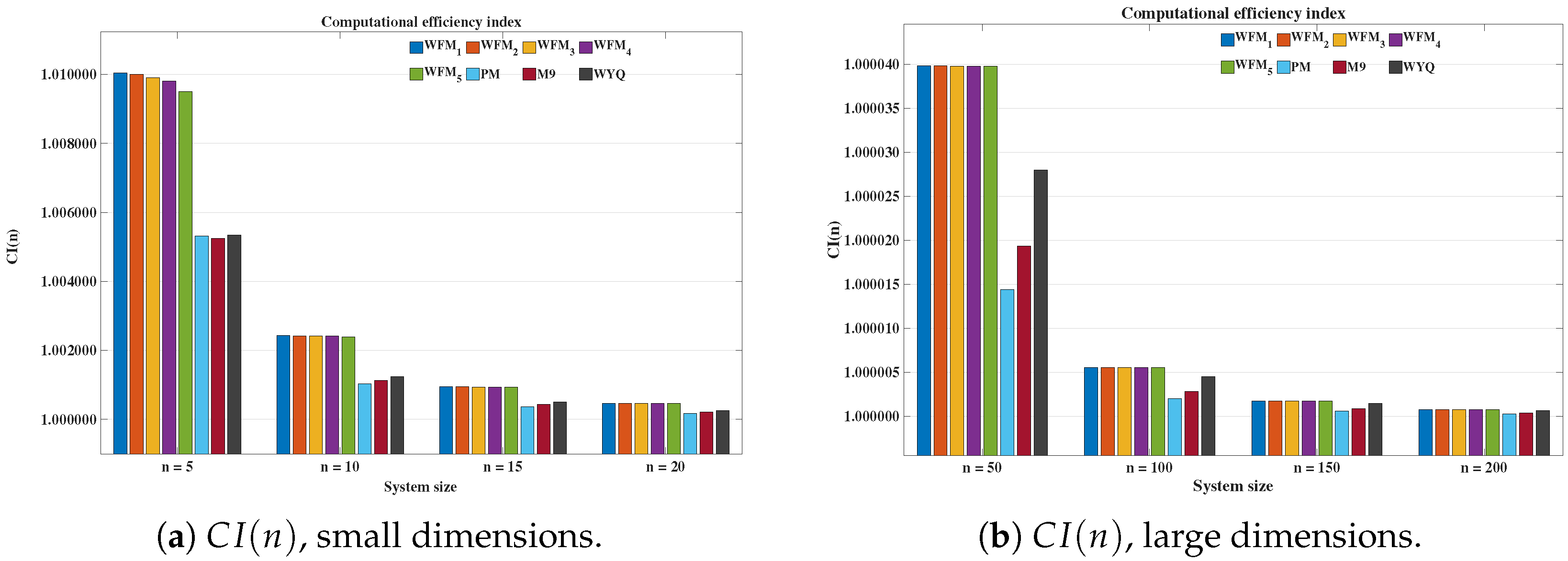
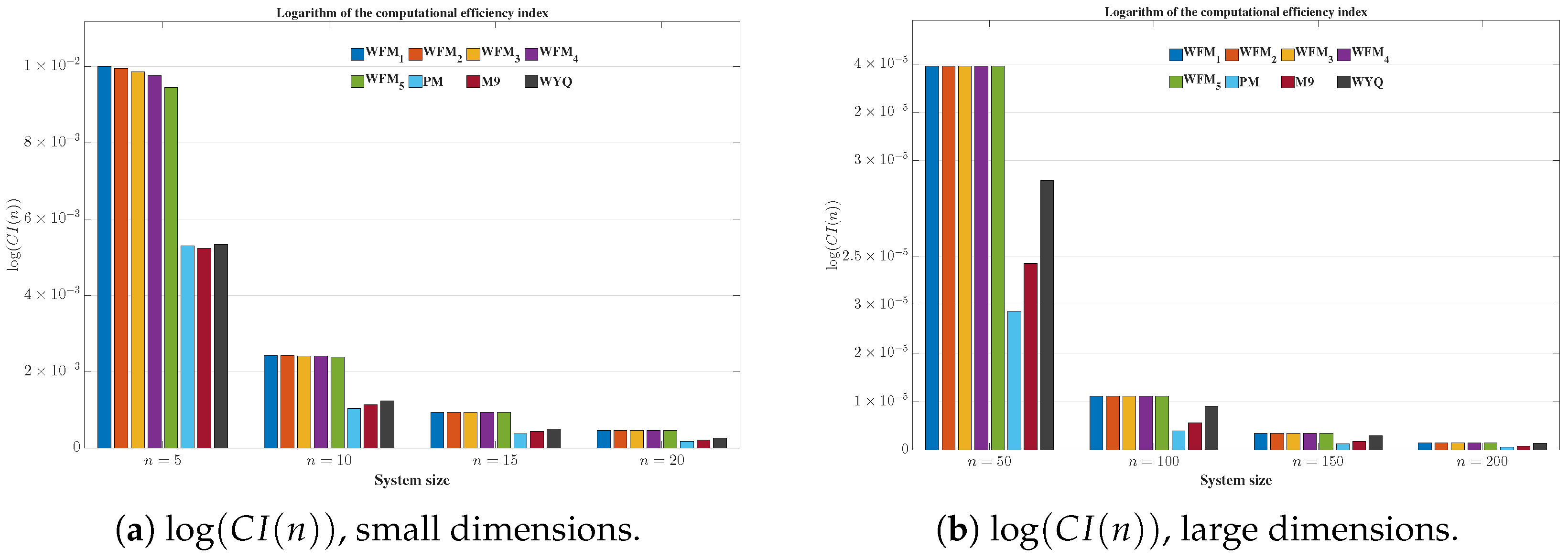
The computational efficiency index $CI\left(n\right)$ for small and large nonlinear systems is shown in Figure 1. The logarithmic representation of this index is presented in Figure 2, which makes the differences between the methods more visible for large dimensions.

As shown in Figure 1a,b and Figure 2a,b, the proposed methods $WF{M}_i$, $i=1,\dots ,5$, consistently attain higher computational efficiency indices than the benchmark methods $PM$, $M9$, and $WYQ$. This superiority is visually reflected in the larger bar heights of the $WF{M}_i$ methods for both small and large systems. The logarithmic plots confirm the same trend, reinforcing the computational advantage of the proposed family under the adopted cost model.

4.3. Test Problems and Numerical Results

In this subsection, we evaluate the numerical performance of ${\mathrm{WFM}}_1$–${\mathrm{WFM}}_5$ and compare them with PM, M9, and WYQ on five nonlinear systems of different dimensions and structures. The selected tests include dense, cyclic, transcendental, and large-scale nonlinear systems, providing a representative framework for assessing accuracy, convergence behavior, and computational cost.

For each method and test problem, the tables report the number of iterations, the norm of the last correction

$$\parallel \Delta x_k\parallel =\parallel x^{(k+1)}-x^{\left(k\right)}\parallel ,$$

the residual norm

$$\parallel F\left(x^{\left(k\right)}\right)\parallel ,$$

the CPU time, and the approximated computational order of convergence (ACOC). A dash symbol, “–”, indicates that the ACOC estimator did not provide a stable representative value in the last iterations.

The stopping criterion used in all tests was

$$\parallel x^{(k+1)}-x^{\left(k\right)}\parallel +\parallel F\left(x^{(k+1)}\right)\parallel <{10}^{-100},$$

with a maximum of 50 iterations. All computations were carried out in MATLAB R2025b Update 5 using vpa (variable-precision arithmetic) through with 2000 decimal digits. This high-precision setting was used to reduce round-off effects and to observe the asymptotic behavior of the methods more reliably.

For each nonlinear system, all methods were tested from the same initial approximation. To obtain representative timing data, each method was executed 10 times, and the CPU time reported in the tables corresponds to the average value. The computations were performed on a computer running macOS Tahoe, version 26.3, equipped with an Apple M2 processor and 8 GB of LPDDR5 RAM.

Example 1.

For the first numerical test, we consider the following nonlinear system of dimension $n=30$:

$$\left\{\begin{array}{c}{x}_1-cos(x_1-x_2-\cdots -x_{30})=0,\hfill \\ x_2-cos(-x_1+x_2-\cdots -x_{30})=0,\hfill \\ ⋮\hfill \\ x_{30}-cos(-x_1-\cdots -x_{29}+x_{30})=0.\hfill \end{array}\right.$$

The initial approximation is taken as

$$x^{\left(0\right)}=(0.2,0.2,\dots ,0.2)\in {\mathbb{R}}^{30}.$$

Example 2.

As a second test problem, we consider a nonlinear system of dimension $n=25$:

$$\left\{\begin{array}{c}{x}_1+5-2log(1+x_2+x_3+\cdots +x_{25})=0,\hfill \\ x_2+5-2log(1+x_1+x_3+\cdots +x_{25})=0,\hfill \\ ⋮\hfill \\ x_{25}+5-2log(1+x_1+x_2+\cdots +x_{24})=0.\hfill \end{array}\right.$$

The starting vector is chosen as

$$x^{\left(0\right)}=(3.5,3.5,\dots ,3.5)\in {\mathbb{R}}^{25}.$$

Example 3.

For the third numerical example, we employ the cyclic logarithmic system with $n=999$:

$$\left\{\begin{array}{c}{x}_1+log(2+x_1+x_2)=0,\hfill \\ x_2+log(2+x_2+x_3)=0,\hfill \\ ⋮\hfill \\ x_{998}+log(2+x_{998}+x_{999})=0,\hfill \\ x_{999}+log(2+x_{999}+x_1)=0.\hfill \end{array}\right.$$

The initial approximation is

$$x^{\left(0\right)}=(0.5,0.5,\dots ,0.5)\in {\mathbb{R}}^{999}.$$

Example 4.

The fourth test problem is the following the atan-quadratic system of dimension $n=100$:

$$4x_i^2+1+arctan\left(x_i\right)-2{\displaystyle \sum _{j=1}^{100}}{x}_j^2=0,i=1,2,\dots ,100.$$

We take as initial approximation

$$x^{\left(0\right)}=(0.1,0.1,\dots ,0.1)\in {\mathbb{R}}^{100}.$$

Example 5.

Finally, we consider the exponential system with dimension $n=99$:

$$\left\{\begin{array}{c}{e}^{-x_1}-(x_2+x_3+\cdots +x_{99})=0,\hfill \\ e^{-x_2}-(x_1+x_3+\cdots +x_{99})=0,\hfill \\ ⋮\hfill \\ e^{-x_{99}}-(x_1+x_2+\cdots +x_{98})=0.\hfill \end{array}\right.$$

The initial vector is selected as

$$x^{\left(0\right)}=(0.8,0.8,\dots ,0.8)\in {\mathbb{R}}^{99}.$$

Table 4. Numerical performance of ${\mathrm{WFM}}_1$–${\mathrm{WFM}}_5$, PM, M9 and WYQ for Example 1.

Method	Iter.	$\parallel \Delta {\mathit{x}}_{\mathit{k}}\parallel$	$\parallel \mathit{F}\left({\mathit{x}}^{\left(\mathit{k}\right)}\right)\parallel$	CPU Time (s)	ACOC
${\mathrm{WFM}}_1$	4	$4.34177\times {10}^{-111}$	$3.38390\times {10}^{-880}$	14.6021772	7.9824550
${\mathrm{WFM}}_2$	4	$2.71356\times {10}^{-114}$	$7.86786\times {10}^{-906}$	15.8159557	7.9849689
${\mathrm{WFM}}_3$	4	$3.81363\times {10}^{-115}$	$1.19743\times {10}^{-912}$	14.6606594	7.9855645
${\mathrm{WFM}}_4$	4	$8.40498\times {10}^{-106}$	$6.68198\times {10}^{-838}$	14.2844560	7.9772471
${\mathrm{WFM}}_5$	4	$7.10282\times {10}^{-119}$	$1.73377\times {10}^{-942}$	14.5347087	7.9878789
PM	4	$4.49464\times {10}^{-341}$	$5.03798\times {10}^{-2507}$	49.0531477	–
M9	4	$2.62603\times {10}^{-255}$	$1.11344\times {10}^{-2288}$	27.8412393	8.9996406
WYQ	4	$8.30052\times {10}^{-124}$	$6.38043\times {10}^{-983}$	20.2921609	7.9728249

,

Table 5. Numerical performance of ${\mathrm{WFM}}_1$–${\mathrm{WFM}}_5$, PM, M9 and WYQ for Example 2.

Method	Iter.	$\parallel \Delta {\mathit{x}}_{\mathit{k}}\parallel$	$\parallel \mathit{F}\left({\mathit{x}}^{\left(\mathit{k}\right)}\right)\parallel$	CPU Time (s)	ACOC
${\mathrm{WFM}}_1$	4	$1.33693\times {10}^{-298}$	$2.55607\times {10}^{-2393}$	7.3797189	7.9999963
${\mathrm{WFM}}_2$	4	$9.58699\times {10}^{-300}$	$1.76127\times {10}^{-2402}$	7.4115643	7.9999965
${\mathrm{WFM}}_3$	4	$7.96911\times {10}^{-300}$	$4.01465\times {10}^{-2403}$	7.1155297	7.9999965
${\mathrm{WFM}}_4$	4	$6.47669\times {10}^{-297}$	$7.86634\times {10}^{-2380}$	6.6652385	7.9999961
${\mathrm{WFM}}_5$	4	$5.14342\times {10}^{-300}$	$1.20888\times {10}^{-2404}$	6.5354908	7.9999965
PM	4	$1.56037\times {10}^{-655}$	$1.05244\times {10}^{-2506}$	9.1727140	–
M9	4	$5.64177\times {10}^{-529}$	$0.0$	11.6027117	–
WYQ	4	$8.76702\times {10}^{-293}$	$8.19136\times {10}^{-2347}$	8.5091259	7.9999950

,

Table 6. Numerical performance of ${\mathrm{WFM}}_1$–${\mathrm{WFM}}_5$, PM, M9 and WYQ for Example 3.

Method	Iter.	$\parallel \Delta {\mathit{x}}_{\mathit{k}}\parallel$	$\parallel \mathit{F}\left({\mathit{x}}^{\left(\mathit{k}\right)}\right)\parallel$	CPU Time (s)	ACOC
${\mathrm{WFM}}_1$	4	$5.65696\times {10}^{-266}$	$2.57927\times {10}^{-2134}$	91.5358244	8.0000099
${\mathrm{WFM}}_2$	4	$3.94752\times {10}^{-286}$	$1.21946\times {10}^{-2295}$	92.2275333	8.0000048
${\mathrm{WFM}}_3$	4	$2.38568\times {10}^{-288}$	$2.17006\times {10}^{-2313}$	95.5582538	8.0000044
${\mathrm{WFM}}_4$	4	$8.26220\times {10}^{-250}$	$6.19040\times {10}^{-2005}$	97.8998805	8.0000174
${\mathrm{WFM}}_5$	4	$4.44332\times {10}^{-278}$	$3.14215\times {10}^{-2231}$	97.0318207	8.0000064
PM	4	$6.32061\times {10}^{-304}$	$2.07902\times {10}^{-2507}$	184.0220661	8.9999796
M9	4	$5.89635\times {10}^{-310}$	$0.0$	153.0867581	8.9999850
WYQ	5	$4.09721\times {10}^{-776}$	$2.07902\times {10}^{-2507}$	142.0091811	–

,

Table 7. Numerical performance of ${\mathrm{WFM}}_1$–${\mathrm{WFM}}_5$, PM, M9 and WYQ for Example 4.

Method	Iter.	$\parallel \Delta {\mathit{x}}_{\mathit{k}}\parallel$	$\parallel \mathit{F}\left({\mathit{x}}^{\left(\mathit{k}\right)}\right)\parallel$	CPU Time (s)	ACOC
${\mathrm{WFM}}_1$	4	$8.26388\times {10}^{-289}$	$7.20686\times {10}^{-2303}$	154.6541409	7.9999968
${\mathrm{WFM}}_2$	4	$2.72474\times {10}^{-289}$	$9.78685\times {10}^{-2307}$	156.6791355	7.9999968
${\mathrm{WFM}}_3$	4	$2.57370\times {10}^{-289}$	$6.20164\times {10}^{-2307}$	155.9149696	7.9999968
${\mathrm{WFM}}_4$	4	$1.51262\times {10}^{-288}$	$9.33277\times {10}^{-2301}$	162.1811436	7.9999967
${\mathrm{WFM}}_5$	4	$6.15445\times {10}^{-290}$	$6.63062\times {10}^{-2312}$	154.6609909	7.9999969
PM	4	$4.79728\times {10}^{-566}$	$2.41144\times {10}^{-2507}$	255.2043015	–
M9	4	$1.04279\times {10}^{-558}$	$2.16965\times {10}^{-2507}$	337.3328560	–
WYQ	4	$2.50127\times {10}^{-275}$	$9.87225\times {10}^{-2195}$	238.3740648	7.9999942

and

Table 8. Numerical performance of ${\mathrm{WFM}}_1$–${\mathrm{WFM}}_5$, PM, M9 and WYQ for Example 5.

Method	Iter.	$\parallel \Delta {\mathit{x}}_{\mathit{k}}\parallel$	$\parallel \mathit{F}\left({\mathit{x}}^{\left(\mathit{k}\right)}\right)\parallel$	CPU Time (s)	ACOC
${\mathrm{WFM}}_1$	3	$4.02268\times {10}^{-106}$	$2.27692\times {10}^{-859}$	88.2883201	7.9428813
${\mathrm{WFM}}_2$	3	$4.02072\times {10}^{-106}$	$2.26774\times {10}^{-859}$	89.6271794	7.9428853
${\mathrm{WFM}}_3$	3	$4.02072\times {10}^{-106}$	$2.26774\times {10}^{-859}$	88.4056499	7.9428853
${\mathrm{WFM}}_4$	3	$4.02424\times {10}^{-106}$	$2.28438\times {10}^{-859}$	90.2564420	7.9428768
${\mathrm{WFM}}_5$	3	$4.02694\times {10}^{-106}$	$2.29594\times {10}^{-859}$	90.3166534	7.9428920
PM	3	$2.25513\times {10}^{-140}$	$4.53730\times {10}^{-1276}$	163.2374083	8.9449643
M9	3	$9.42805\times {10}^{-141}$	$1.57088\times {10}^{-1279}$	225.2958072	8.9462051
WYQ	3	$7.89231\times {10}^{-124}$	$7.19923\times {10}^{-1003}$	153.4825977	7.9408362

collect the numerical performance of ${\mathrm{WFM}}_1$–${\mathrm{WFM}}_5$, PM, M9 and WYQ for the nonlinear systems described in Examples 1–5. The purpose of these experiments is to compare not only final accuracy and observed convergence order but also the computational time required to reach the prescribed tolerance.

The results in Table 4 show that all methods solve the first problem with very high accuracy. The proposed WFM methods reach the prescribed tolerance in four iterations, with ACOC values close to the theoretical order of eight. Although PM and M9 attain smaller final residuals, their CPU times are considerably larger. In particular, ${\mathrm{WFM}}_1$–${\mathrm{WFM}}_5$ require approximately 14–16 s, whereas PM, M9 and WYQ require approximately 49, 28 and 20 s, respectively. Therefore, for this test, the proposed weight-function family provides a favorable balance between accuracy, observed convergence order and computational cost.

For Example 2, Table 5 shows that all WFM methods converge in four iterations and their ACOC values confirm the eighth local order established in Theorem 1. They also require lower CPU times than the reference methods. In particular, ${\mathrm{WFM}}_4$ and ${\mathrm{WFM}}_5$ are the fastest variants, with approximately $6.7$ and $6.5$ s, respectively, compared with $9.2$, $11.6$, and $8.5$ s for PM, M9, and WYQ. Hence, the proposed schemes preserve high accuracy while reducing computational time.

Table 6 shows the results for the large-scale cyclic logarithmic system with $n=999$. The WFM methods converge in four iterations and their ACOC values confirm the eighth local order established in Theorem 1. In terms of CPU time, the proposed schemes require about 91–98 s, clearly improving on PM, M9 and WYQ, which require approximately 184, 153 and 142 s, respectively. Hence, the WFM family is especially competitive for this large-scale problem.

The results in Table 7 show that the proposed methods also perform well on the atan-quadratic system. All WFM variants converge in four iterations and produce ACOC values practically equal to eight. Their CPU times are significantly lower than those of the comparison methods: the WFM schemes take approximately 155–162 s, whereas PM, M9 and WYQ require about 255, 337 and 238 s, respectively. Hence, although the reference methods reach very small residuals, the weight-function family achieves the required accuracy with a substantially lower computational cost.

For the exponential system in Example 5, Table 8 shows that all methods converge in three iterations. The WFM schemes require approximately 88–90 s, whereas PM, M9 and WYQ require about 163, 225 and 153 s, respectively, showing a clear advantage in CPU time.

Overall, Table 4, Table 5, Table 6, Table 7 and Table 8 confirm that the proposed WFM methods are highly competitive. They achieve high accuracy in terms of correction norms and residuals, while consistently requiring less CPU time than the reference schemes.

Numerical Test on a Fredholm Integral Equation

We complement the previous algebraic tests by considering a nonlinear Fredholm integral equation. After quadrature discretization, this problem leads to a dense nonlinear algebraic system whose structure differs from the polynomial, transcendental, and cyclic systems analyzed above. Therefore, it provides an additional benchmark for assessing the practical behavior of the proposed methods ${\mathrm{WFM}}_1$–${\mathrm{WFM}}_5$ and the reference schemes PM, M9, and WYQ.

Example 6

(Nonlinear Fredholm integral equation). We consider the nonlinear Fredholm integral equation of the second kind,

$$y\left(t\right)={\displaystyle \frac{t}{e}}+{\int }_0^{1}2ts{e}^{-y{\left(s\right)}^2}ds,t\in [0,1].$$

(48)

This problem has been used as a benchmark in the numerical analysis of high-order iterative methods for nonlinear systems [7]. Moreover, the continuous problem admits the exact solution,

$$y\left(t\right)=t,$$

since

$${\displaystyle \frac{t}{e}}+{\int }_0^{1}2ts{e}^{-s^2}ds={\displaystyle \frac{t}{e}}+t(1-e^{-1})=t.$$

For the numerical discretization, we take $m=50$ and introduce the uniform nodes

$$t_j={\displaystyle \frac{j}{m}},j=1,\dots ,m.$$

The integral in (48) is approximated by the composite Simpson rule. Since $m=50$ is even, the rule can be applied directly. The unknowns are denoted by

$$y_j\approx y\left(t_j\right),j=1,\dots ,m,$$

and we write

$$Y={(y_1,\dots ,y_m)}^T.$$

The node $t_0=0$ is not included as an unknown because the factor s in the kernel makes its contribution vanish. Thus, the discretization of (48) gives the nonlinear algebraic system

$$F_i\left(Y\right)=y_i-{\displaystyle \frac{t_i}{e}}-2t_i{\displaystyle \sum _{j=1}^m}{p}_j{t}_j{e}^{-y_j^2}=0,i=1,\dots ,m,$$

(49)

where the Simpson weights are given by

$$p_j=\left\{\begin{array}{cc}{\displaystyle \frac{4h}{3}},\hfill & j\mathit{odd},j<m,\hfill \\ {\displaystyle \frac{2h}{3}},\hfill & j\mathit{even},j<m,\hfill \\ {\displaystyle \frac{h}{3}},\hfill & j=m,\hfill \end{array}\right.h={\displaystyle \frac{1}{m}}.$$

The Jacobian matrix associated with (49) is

$${\displaystyle \frac{\partial F_i}{\partial y_{\ell }}}\left(Y\right)={\delta }_{i\ell }+4t_i{p}_{\ell }{t}_{\ell }{y}_{\ell }{e}^{-y_{\ell }^2},i,\ell =1,\dots ,m,$$

(50)

where ${\delta }_{i\ell }$ denotes the Kronecker delta.

In the numerical experiment, all methods are initialized with

$$Y^{\left(0\right)}={(0,0,\dots ,0)}^T\in {\mathbb{R}}^{50}.$$

The stopping criterion, tolerance, maximum number of iterations, precision setting, CPU-time averaging procedure, and ACOC estimator are the same as those described in Section 4.3.

The computed discrete solution can be represented in compact form as

$$Y^{*}\approx c_{50}{\left({\displaystyle \frac{1}{50}},{\displaystyle \frac{2}{50}},\dots ,{\displaystyle \frac{50}{50}}\right)}^T,c_{50}\approx 1.00000001126261.$$

In particular,

$$y_1^{*}\approx 0.0200000002252521,y_{50}^{*}\approx 1.00000001126261.$$

The resulting nonlinear system has a dimension of 50 and dense coupling induced by the quadrature approximation of the integral term. This makes the problem suitable for comparing the robustness and efficiency of ${\mathrm{WFM}}_1$–${\mathrm{WFM}}_5$ against PM, M9, and WYQ.

For this Fredholm test problem,

Table 9. Numerical performance of ${\mathrm{WFM}}_1$–${\mathrm{WFM}}_5$, PM, M9, and WYQ for the nonlinear Fredholm integral equation with $m=50$.

Method	Iter.	$\parallel {\mathit{Y}}^{(\mathit{k}+1)}-{\mathit{Y}}^{\left(\mathit{k}\right)}\parallel$	$\parallel \mathit{F}\left({\mathit{Y}}^{\left(\mathit{k}\right)}\right)\parallel$	CPU Time (s)	ACOC
${\mathrm{WFM}}_1$	4	$1.12322543695\times {10}^{-108}$	$1.03546797078\times {10}^{-872}$	11.12287521	8.0107943
${\mathrm{WFM}}_2$	4	$2.82920330342\times {10}^{-111}$	$1.67745050493\times {10}^{-893}$	10.87682979	8.0097596
${\mathrm{WFM}}_3$	4	$6.95879720136\times {10}^{-112}$	$2.24703534500\times {10}^{-898}$	11.93490308	8.0095350
${\mathrm{WFM}}_4$	4	$1.48233008770\times {10}^{-111}$	$9.52567704478\times {10}^{-896}$	11.52577850	8.0096581
${\mathrm{WFM}}_5$	4	$9.71861985888\times {10}^{-117}$	$3.25216988450\times {10}^{-937}$	11.10030508	8.0079084
PM	4	$7.38645890536\times {10}^{-275}$	$3.38270418458\times {10}^{-2008}$	23.60907583	9.0002903
M9	4	$9.71886924553\times {10}^{-246}$	$3.62112819870\times {10}^{-2008}$	36.75360204	9.0007835
WYQ	4	$1.72784769587\times {10}^{-157}$	$9.72776605319\times {10}^{-1265}$	22.82704475	8.0102103

reports the main numerical output of each method: the number of iterations, the norm of the final increment $\parallel Y^{(k+1)}-Y^{\left(k\right)}\parallel$, the final residual norm $\parallel F\left(Y^{\left(k\right)}\right)\parallel$, the averaged CPU time, and the ACOC value.

The results in Table 9 show that all methods solve the Fredholm test problem with very small final increments and residual norms. The proposed ${\mathrm{WFM}}_1$–${\mathrm{WFM}}_5$ schemes converge in four iterations and exhibit ACOC values that confirm the eighth local order established in Theorem 1. Although PM and M9 achieve smaller residuals, their CPU times are substantially larger. In particular, the WFM methods require approximately 11–12 s, whereas PM, M9, and WYQ require approximately $23.6$, $36.8$, and $22.8$ s, respectively. Thus, the proposed family provides a favorable balance between accuracy, confirmed local order, and computational time for this dense Fredholm discretization.

5. Application to a Semilinear Elliptic Dirichlet Problem

This section validates the proposed methods on a two-dimensional semilinear elliptic Dirichlet problem. This benchmark is suitable because it is genuinely nonlinear, has a smooth manufactured exact solution, and leads to a sparse Jacobian matrix with a clear structure. It also allows a direct comparison between the approximate and exact solutions through three-dimensional plots.

The test is used to evaluate the five selected members of the proposed weight-function family, ${\mathrm{WFM}}_1$–${\mathrm{WFM}}_5$, together with the benchmark methods PM, M9, and WYQ considered in the previous section. The validation follows the standard manufactured-solution approach [15,16], and the spatial discretization is based on the classical five-point finite-difference stencil for elliptic problems [17,18].

5.1. Model Problem and Manufactured Exact Solution

Let

$$\Omega =(0,1)\times (0,1),\partial \Omega =\mathrm{boundary}\mathrm{of}\Omega .$$

We consider the semilinear Dirichlet problem

$$-\Delta u(x,y)+u{(x,y)}^3=f(x,y),(x,y)\in \Omega ,$$

(51)

subject to the homogeneous boundary condition

$$u(x,y)=0,(x,y)\in \partial \Omega .$$

(52)

Here,

$$\Delta u=u_{xx}+u_{yy}$$

denotes the Laplacian operator. The cubic reaction term makes (51) nonlinear, while the resulting Jacobian matrix after discretization remains sparse and easy to assemble.

For validation purposes, we prescribe the manufactured exact solution

$$u(x,y)=sin\left(\pi x\right)sin\left(\pi y\right).$$

(53)

This function satisfies (52) since it vanishes on each side of the unit square. Moreover,

$$-\Delta u(x,y)=2{\pi }^{2}sin\left(\pi x\right)sin\left(\pi y\right),$$

and substitution of (53) into (51) yields the compatible forcing term

$$f(x,y)=2{\pi }^{2}sin\left(\pi x\right)sin\left(\pi y\right)+{sin}^3\left(\pi x\right){sin}^3\left(\pi y\right).$$

(54)

Consequently, Equation (53) is the exact solution of (51) and (52). This construction provides a rigorous framework for measuring both nonlinear solver performance and discretization accuracy [15,16].

5.2. Finite-Difference Discretization

Let N be the number of interior nodes in each coordinate direction, and define the uniform mesh

$$x_i=ih,y_j=jh,i,j=0,1,\dots ,N+1,h={\displaystyle \frac{1}{N+1}}.$$

The unknowns are the interior nodal values

$$u_{i,j}\approx u(x_i,y_j),1\le i,j\le N,$$

whereas the boundary values are imposed by (52). Since the exact solution vanishes on $\partial \Omega$, the discrete boundary data are also zero.

• Using the standard five-point approximation of the Laplacian, one has

$$-\Delta u(x_i,y_j)={\displaystyle \frac{4u_{i,j}-u_{i-1,j}-u_{i+1,j}-u_{i,j-1}-u_{i,j+1}}{h^2}}+\mathcal{O}\left(h^2\right),$$

(55)

for $1\le i,j\le N$. Therefore, the discrete counterpart of (51) is

$${\displaystyle \frac{4u_{i,j}-u_{i-1,j}-u_{i+1,j}-u_{i,j-1}-u_{i,j+1}}{h^2}}+u_{i,j}^3-f(x_i,y_j)=0,$$

(56)

for $1\le i,j\le N$. For smooth solutions, the spatial discretization is second-order consistent, as follows directly from (55); see [17,18].

5.3. Nonlinear Algebraic System and Jacobian

To write the discrete problem in compact form, let

$$U={\left(u_{1,1},u_{2,1},\dots ,u_{N,1},u_{1,2},u_{2,2},\dots ,u_{N,N}\right)}^T\in {\mathbb{R}}^{N^2}$$

be the vector of unknown nodal values in lexicographic order. Let $I_N$ denote the $N\times N$ identity matrix, and define

$$T_N=\left(\begin{array}{ccccc}2& -1& 0& \dots & 0\\ -1& 2& -1& \ddots & ⋮\\ 0& -1& 2& \ddots & 0\\ ⋮& \ddots & \ddots & \ddots & -1\\ 0& \dots & 0& -1& 2\end{array}\right).$$

Then, the matrix associated with the negative discrete Laplacian is

$$A_h={\displaystyle \frac{1}{h^2}}\left(I_N\otimes T_N+T_N\otimes I_N\right)\in {\mathbb{R}}^{N^2\times N^2},$$

(57)

where ⊗ denotes the Kronecker product. Let

$$F_h={\left(f(x_1,y_1),f(x_2,y_1),\dots ,f(x_N,y_N)\right)}^T$$

be the vector of source values, and define the componentwise cubic vector

$$U^{\left[3\right]}={\left(u_1^3,u_2^3,\dots ,u_{N^2}^3\right)}^T.$$

Since the Dirichlet data are homogeneous, no additional boundary correction terms are needed. Hence, the discrete problem can be written as

$$F\left(U\right)=A_{h}U+U^{\left[3\right]}-F_h=0.$$

(58)

Equation (58) is the nonlinear algebraic system to which the methods ${\mathrm{WFM}}_1$–${\mathrm{WFM}}_5$, PM, M9, and WYQ are applied.

The Jacobian matrix associated with (58) is

$$J\left(U\right)=F^{\prime }\left(U\right)=A_h+3\mathrm{diag}\left(U^{\left[2\right]}\right),$$

(59)

where

$$U^{\left[2\right]}={\left(u_1^2,u_2^2,\dots ,u_{N^2}^2\right)}^T.$$

In nodewise form, the nonzero partial derivatives are

$${\displaystyle \frac{\partial F_{i,j}}{\partial u_{i,j}}}={\displaystyle \frac{4}{h^2}}+3u_{i,j}^2,$$

(60)

and

$${\displaystyle \frac{\partial F_{i,j}}{\partial u_{i\pm 1,j}}}=-{\displaystyle \frac{1}{h^2}},{\displaystyle \frac{\partial F_{i,j}}{\partial u_{i,j\pm 1}}}=-{\displaystyle \frac{1}{h^2}}.$$

(61)

All other partial derivatives vanish. Therefore, $J\left(U\right)$ is sparse, symmetric, and block tridiagonal. Since $A_h$ is symmetric positive-definite and $3\mathrm{diag}\left(U^{\left[2\right]}\right)$ is nonnegative diagonal, the Jacobian remains symmetric positive definite for a real U, which is favorable for repeated linear solves within high-order Newton-type schemes.

5.4. Error Measures and Numerical Protocol

Since the manufactured exact solution is available, the accuracy of the computed discrete solution can be assessed directly. For this reason, we report both $E_{\infty ,h}$ and $E_{2,h}$. The norm $E_{\infty ,h}$ measures the maximum pointwise error over the computational grid, whereas $E_{2,h}$ provides a global discrete error measure. These two quantities complement the residual norm since a small nonlinear residual indicates that the discrete algebraic system has been solved accurately, while $E_{\infty ,h}$ and $E_{2,h}$ quantify the actual discrepancy between the numerical approximation and the manufactured exact solution.

$$E_{\infty ,h}=\underset{1\le i,j\le N}{max}\left|u_{i,j}^{\left(h\right)}-u(x_i,y_j)\right|,$$

(62)

and

$$E_{2,h}=h{\left({\displaystyle \sum _{i=1}^N}{\displaystyle \sum _{j=1}^N}{\left|u_{i,j}^{\left(h\right)}-u(x_i,y_j)\right|}^2\right)}^{1/2}.$$

(63)

For each iterative scheme, we also report the residual norm, $\parallel F\left(U^{\left(k\right)}\right){\parallel }_2$, the norm of the last increment,

$$\parallel \Delta U_k{\parallel }_2={\parallel U^{(k+1)}-U^{\left(k\right)}\parallel }_2,$$

the elapsed CPU time, and the number of iterations.

In the numerical implementation, two uniform meshes were considered. First, we used

$$N=20,h={\displaystyle \frac{1}{21}},dim\left(F\right)=N^2=400.$$

In addition, to assess the effect of mesh refinement on the spatial discretization error, we also considered the finer mesh

$$N=40,h={\displaystyle \frac{1}{41}},dim\left(F\right)=N^2=1600.$$

Thus, the first mesh is used to compare the nonlinear solvers under a moderate problem size, whereas the second one allows us to verify the expected reduction in the spatial errors $E_{\infty ,h}$ and $E_{2,h}$.

All methods were initialized with the same starting vector

$$U^{\left(0\right)}={\displaystyle \frac{1}{2}}{U}_{\mathrm{exact},h},$$

that is,

$$u_{i,j}^{\left(0\right)}={\displaystyle \frac{1}{2}}sin\left(\pi x_i\right)sin\left(\pi y_j\right),1\le i,j\le N.$$

The stopping criterion was

$$\parallel U^{(k+1)}-U^{\left(k\right)}{\parallel }_2+{\parallel F\left(U^{(k+1)}\right)\parallel }_2<{10}^{-100},$$

(64)

with a maximum of 50 nonlinear iterations. All computations were performed in MATLAB R2025b Update 5 using variable-precision arithmetic with 1000 decimal digits, set through digits(1000) and implemented with vpa. The methods tested were ${\mathrm{WFM}}_1,\dots ,{\mathrm{WFM}}_5$, PM, M9, and WYQ.

5.5. Numerical Results

The nonlinear system (58) was solved using the numerical protocol described in Section 5.4. Since the manufactured exact solution is known, this test evaluates both the algebraic behavior of the iterative methods and the accuracy of the discrete approximation.

Table 10. Numerical results for the manufactured semilinear elliptic problem.

Method	Iter.	$\parallel \Delta {\mathit{U}}_{\mathit{k}}{\parallel }_2$	$\parallel \mathit{F}\left({\mathit{U}}^{\left(\mathit{k}\right)}\right){\parallel }_2$	${\mathit{E}}_{\mathit{\infty },\mathit{h}}$	${\mathit{E}}_{2,\mathit{h}}$	CPU Time (s)
${\mathrm{WFM}}_1$	5	$1.420311\times {10}^{-327}$	$3.930009\times {10}^{-655}$	$1.689721\times {10}^{-3}$	$8.600762\times {10}^{-4}$	20.547
${\mathrm{WFM}}_2$	5	$1.420838\times {10}^{-327}$	$3.932924\times {10}^{-655}$	$1.689721\times {10}^{-3}$	$8.600762\times {10}^{-4}$	20.102
${\mathrm{WFM}}_3$	5	$1.420861\times {10}^{-327}$	$3.933052\times {10}^{-655}$	$1.689721\times {10}^{-3}$	$8.600762\times {10}^{-4}$	20.073
${\mathrm{WFM}}_4$	5	$1.417920\times {10}^{-327}$	$3.916785\times {10}^{-655}$	$1.689721\times {10}^{-3}$	$8.600762\times {10}^{-4}$	19.993
${\mathrm{WFM}}_5$	5	$1.467772\times {10}^{-327}$	$4.197114\times {10}^{-655}$	$1.689721\times {10}^{-3}$	$8.600762\times {10}^{-4}$	20.079
PM	4	$3.051726\times {10}^{-427}$	$2.276236\times {10}^{-1004}$	$1.689721\times {10}^{-3}$	$8.600762\times {10}^{-4}$	39.309
M9	4	$1.184028\times {10}^{-450}$	$2.363936\times {10}^{-1004}$	$1.689721\times {10}^{-3}$	$8.600762\times {10}^{-4}$	52.201
WYQ	4	$9.203198\times {10}^{-331}$	$2.590885\times {10}^{-1004}$	$1.689721\times {10}^{-3}$	$8.600762\times {10}^{-4}$	38.325

reports, for each method, the number of iterations, the final increment norm, the residual norm, the discrete errors $E_{\infty ,h}$ and $E_{2,h}$, and the CPU time.

The results in Table 10 show that all methods converge to the same discrete solution, as reflected by the identical values of $E_{\infty ,h}$ and $E_{2,h}$. These errors are associated with the finite-difference spatial discretization and are consistent with the second-order accuracy of the five-point stencil. The proposed WFM methods require five iterations and achieve residual norms of order ${10}^{-655}$, with CPU times close to 20 s. In comparison, PM, M9, and WYQ require four iterations and attain smaller residual norms, but with higher CPU times. Thus, the WFM family provides the lowest computational cost in this semilinear elliptic test while preserving the same discrete accuracy.

The results in

Table 11. Numerical results for the manufactured semilinear elliptic problem using a finer mesh.

Method	Iter.	$\parallel \Delta {\mathit{U}}_{\mathit{k}}{\parallel }_2$	$\parallel \mathit{F}\left({\mathit{U}}^{\left(\mathit{k}\right)}\right){\parallel }_2$	${\mathit{E}}_{\mathit{\infty },\mathit{h}}$	${\mathit{E}}_{2,\mathit{h}}$	CPU Time (s)
${\mathrm{WFM}}_1$	5	$8.592136\times {10}^{-328}$	$7.366136\times {10}^{-656}$	$4.448158\times {10}^{-4}$	$2.254952\times {10}^{-4}$	283.420
${\mathrm{WFM}}_2$	5	$8.595397\times {10}^{-328}$	$7.371722\times {10}^{-656}$	$4.448158\times {10}^{-4}$	$2.254952\times {10}^{-4}$	274.840
${\mathrm{WFM}}_3$	5	$8.595533\times {10}^{-328}$	$7.371957\times {10}^{-656}$	$4.448158\times {10}^{-4}$	$2.254952\times {10}^{-4}$	275.390
${\mathrm{WFM}}_4$	5	$8.578062\times {10}^{-328}$	$7.342014\times {10}^{-656}$	$4.448158\times {10}^{-4}$	$2.254952\times {10}^{-4}$	273.960
${\mathrm{WFM}}_5$	5	$8.874080\times {10}^{-328}$	$7.857610\times {10}^{-656}$	$4.448158\times {10}^{-4}$	$2.254952\times {10}^{-4}$	273.860
PM	4	$1.341335\times {10}^{-427}$	$1.823340\times {10}^{-1003}$	$4.448158\times {10}^{-4}$	$2.254952\times {10}^{-4}$	518.610
M9	4	$6.616362\times {10}^{-451}$	$1.810786\times {10}^{-1003}$	$4.448158\times {10}^{-4}$	$2.254952\times {10}^{-4}$	678.670
WYQ	4	$2.639372\times {10}^{-331}$	$1.742113\times {10}^{-1003}$	$4.448158\times {10}^{-4}$	$2.254952\times {10}^{-4}$	449.740

correspond to a finer spatial mesh. As expected, the spatial errors $E_{\infty ,h}$ and $E_{2,h}$ are smaller than those obtained with the coarser mesh. The WFM methods require five iterations and achieve residual norms of order ${10}^{-656}$, with lower CPU times than PM, M9, and WYQ. Thus, even for the larger discretized system, the proposed WFM family preserves competitive accuracy and computational efficiency.

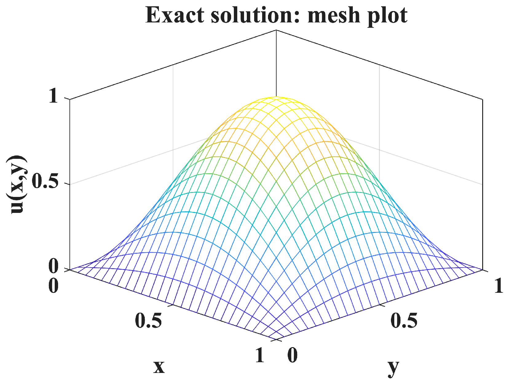
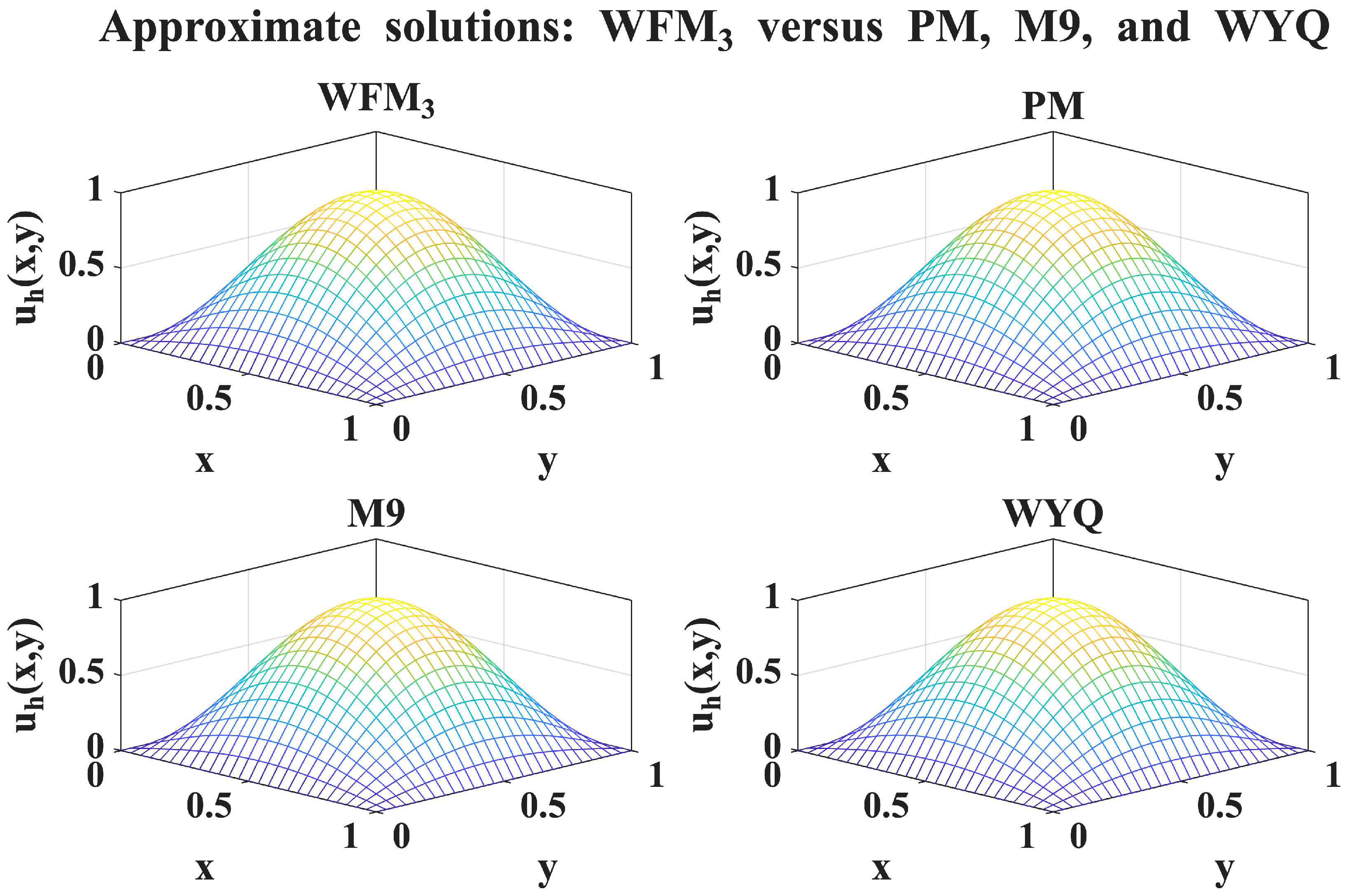
The graphical results displayed in Figure 3 and Figure 4 confirm that the representative approximate solutions reproduce the qualitative shape of the manufactured exact solution, with small error levels throughout the computational domain.

6. Conclusions

The numerical experiments carried out in this work support the theoretical performance of the proposed schemes on nonlinear systems of different dimensions and structures. In addition, the proposed weight-function family generalizes the original CTT8 method, which is recovered as a particular member through a suitable choice of the weight functions. Therefore, the present construction extends the CTT8 scheme from an isolated optimal eighth-order method to a broader family of optimal iterative procedures for nonlinear systems.

The new schemes are competitive in terms of residual accuracy, correction norm, and computational efficiency. The Fredholm integral equation and the semilinear elliptic Dirichlet problem further illustrate the reliability and computational performance of the methods when applied to nonlinear systems arising from numerical discretizations.

The theoretical contribution of the paper can be summarized as follows. Starting from a Newton-type predictor and a fourth-order correction, we introduced a third correction step governed by multivariable scalar weight functions. Suitable Taylor conditions on these functions were derived in order to cancel all error terms up to order seven. As a consequence, the resulting schemes attain eighth-order local convergence for nondegenerate solutions. Since the methods require one Jacobian evaluation and three evaluations of the nonlinear operator per iteration, they attain the Cordero–Torregrosa optimal bound for nonlinear systems.

The use of weight functions is important because it changes the role of the original CTT8 method. Instead of having a single eighth-order optimal scheme, the proposed construction provides a whole admissible family. This makes it possible to introduce polynomial, exponential, rational, and parametric perturbations without increasing the number of evaluations of F or $F^{\prime }$. Therefore, the weight-function framework offers flexibility while preserving the same optimal convergence structure.

From the computational point of view, the cost analysis shows that the proposed WFM methods have a favorable efficiency profile when compared with the reference schemes PM, M9, and WYQ. The performance curves for small and large dimensions confirm that the proposed methods preserve eighth-order convergence with a lower asymptotic cost, mainly because they reuse a single Jacobian factorization throughout the iteration. Among the selected members, WFM1 has the lowest algebraic overhead, whereas the remaining WFM variants illustrate that more elaborate admissible weight functions can be incorporated with only a small constant increase in cost.

The numerical examples confirm the theoretical conclusions. For the finite-dimensional nonlinear test systems, the proposed methods reach very small correction norms and residual norms, and the observed values of the approximated computational order of convergence agree with the expected eighth order. These results indicate that the theoretical error analysis is reflected in the practical behavior of the schemes.

The Fredholm integral equation provides a relevant test because its quadrature discretization leads to dense nonlinear algebraic systems. In this setting, the proposed WFM methods maintain high accuracy and competitive CPU times, showing that the family is not restricted to artificial low-dimensional examples. The semilinear elliptic Dirichlet problem gives an additional and more demanding validation, since the finite-difference discretization generates structured nonlinear systems whose size increases with mesh refinement. The results obtained for both coarse and finer meshes show that the proposed methods reproduce the manufactured solution with small spatial errors and robust residual reduction.

Overall, the proposed family combines three desirable properties: optimal eighth-order convergence, computational efficiency, and flexibility through admissible weight functions. Future work may focus on semilocal convergence, the adaptive selection of weight functions, implementation for sparse and large-scale systems, and the extension of the proposed framework to problems with singular or nearly singular Jacobians, as well as to nonlinear systems arising from time-dependent partial differential equations.

References

1. Traub, J.F. Iterative Methods for the Solution of Equations; Prentice-Hall: Englewood Cliffs, NJ, USA, 1964. [Google Scholar]
2. Ortega, J.M.; Rheinboldt, W.C. Iterative Solution of Nonlinear Equations in Several Variables; Academic Press: New York, NY, USA, 1970. [Google Scholar]
3. Kung, H.T.; Traub, J.F. Optimal order of one-point and multi-point iteration. J. ACM 1974, 21, 643–651. [Google Scholar] [CrossRef] [Scilit]
4. Arroyo, V.; Cordero, A.; Torregrosa, J.R. Approximation of artificial satellites’ preliminary orbits: The efficiency challenge. Math. Comput. Model. 2011, 54, 1802–1807. [Google Scholar] [CrossRef] [Scilit]
5. Cordero, A.; Torregrosa, J.R.; Triguero-Navarro, P. First Optimal Vectorial Eighth-Order Iterative Scheme for Solving Non-Linear Systems. Appl. Math. Comput. 2025, 498, 129401. [Google Scholar] [CrossRef] [Scilit]
6. Sharma, J.R.; Arora, H. Efficient Jarratt-like Methods for Solving Systems of Nonlinear Equations. Calcolo 2014, 51, 193–210. [Google Scholar] [CrossRef] [Scilit]
7. Hueso, J.L.; Martínez, E.; Teruel, C. Convergence, Efficiency and Dynamics of New Fourth and Sixth Order Families of Iterative Methods for Nonlinear Systems. J. Comput. Appl. Math. 2015, 275, 412–420. [Google Scholar] [CrossRef] [Scilit]
8. Xiao, X.Y. New Techniques to Develop Higher Order Iterative Methods for Systems of Nonlinear Equations. Comput. Appl. Math. 2022, 41, 243. [Google Scholar] [CrossRef] [Scilit]
9. Behl, R.; Bhalla, S.; Magreñán, Á.A.; Kumar, S. An efficient high order iterative scheme for large nonlinear systems with dynamics. J. Comput. Appl. Math. 2022, 404, 113249. [Google Scholar] [CrossRef] [Scilit]
10. Wang, X.; Yang, Y.; Qin, Y. Semilocal convergence analysis of an eighth order iterative method for solving nonlinear systems. AIMS Math. 2023, 8, 22371–22384. [Google Scholar] [CrossRef] [Scilit]
11. Zhang, L.; Wu, Q.B.; Chen, M.H.; Lin, R.F. Two New Effective Iteration Methods for Nonlinear Systems with Complex Symmetric Jacobian Matrices. Comput. Appl. Math. 2021, 40, 250. [Google Scholar] [CrossRef] [Scilit]
12. Cordero, A.; Leonardo Sepúlveda, M.A.; Torregrosa, J.R.; Rodríguez-Cabral, A.; Vassileva, M.P. Generalized Traub Family for Solving Nonlinear Systems: Fourth-Order Optimal Method and Dynamical Analysis. Mathematics 2026, 14, 1161. [Google Scholar] [CrossRef] [Scilit]
13. Sharma, J.R.; Guha, R.K.; Sharma, R. An efficient fourth order weighted-Newton method for systems of nonlinear equations. Numer. Algorithms 2013, 62, 307–323. [Google Scholar] [CrossRef] [Scilit]
14. Cordero, A.; Torregrosa, J.R. Variants of Newton’s method using fifth-order quadrature formulas. Appl. Math. Comput. 2007, 190, 686–698. [Google Scholar] [CrossRef] [Scilit]
15. Roache, P.J. Code Verification by the Method of Manufactured Solutions. J. Fluids Eng. 2002, 124, 4–10. [Google Scholar] [CrossRef] [Scilit]
16. Oberkampf, W.L.; Roy, C.J. Verification and Validation in Scientific Computing; Cambridge University Press: Cambridge, UK, 2010. [Google Scholar]
17. LeVeque, R.J. Finite Difference Methods for Ordinary and Partial Differential Equations: Steady-State and Time-Dependent Problems; Society for Industrial and Applied Mathematics: Philadelphia, PA, USA, 2007. [Google Scholar]
18. Li, Z.; Qiao, Z.; Tang, T. Finite Difference Methods for 2D Elliptic PDEs. In Numerical Solution of Differential Equations: Introduction to Finite Difference and Finite Element Methods; Cambridge University Press: Cambridge, UK, 2017; pp. 47–77. [Google Scholar] [CrossRef] [Scilit]
Figure 1. Computational efficiency index for small and big systems nonlinear equations.
Mathematics 14 02114 g001
Figure 2. Computational efficiency index and its logarithmic representation for the methods under comparison.
Mathematics 14 02114 g002
Figure 3. Exact solution.
Mathematics 14 02114 g003
Figure 4. Approximate solutions obtained with WFM3, PM, M9, and WYQ.
Mathematics 14 02114 g004