Surface Settlement Prediction in Goaf Areas Based on the Improved Radial Movement Optimization–Variational Mode Decomposition–Gated Recurrent Unit Model

Abstract

To solve the low-precision prediction problem of noisy non-stationary goaf subsidence sequences, this study aims to establish a high-accuracy hybrid prediction model for mining surface deformation monitoring. The Global Navigation Satellite System (GNSS) monitoring data of surface subsidence in goaf areas exhibits non-stationary and noisy characteristics, which limits the accuracy of traditional prediction models. In this paper, a hybrid prediction model, namely the Improved Radial Movement Optimization–Variational Mode Decomposition–Gated Recurrent Unit (IRMO-VMD-GRU) model, is proposed. The IRMO algorithm is employed to globally optimize the key parameters of VMD, achieving adaptive and stable decomposition of the settlement sequences. The obtained Intrinsic Mode Function (IMF) sub-sequences are input into the GRU network for independent training and prediction, followed by superposition and reconstruction. The model is validated using the GNSS monitoring data from three monitoring points at a coal mine in Shaanxi Province, China. The results show that the proposed model outperforms the comparison models in all four evaluation indicators, namely Mean Absolute Error (MAE), Root Mean Square Error (RMSE), Mean Absolute Percentage Error (MAPE), and Coefficient of Determination (R²), with all R² values exceeding 0.8. The model demonstrates superior fitting performance, correlation, and generalization ability, which provides important practical technical support for goaf subsidence early warning, geological disaster prevention and engineering safety management in mining areas.

1. Introduction

Surface settlement prediction is a crucial research issue for mining safety and geological disaster prevention, aiming to characterize ground deformation laws induced by underground coal mining. Recent studies have continued to address various engineering challenges in mining areas [1,2,3], highlighting persistent research attention on mining-induced ground stability. Common monitoring methods include traditional leveling, InSAR, and GNSS monitoring, among which GNSS has been widely adopted due to its high precision and continuous observation capability.

The exploitation of coal resources plays a vital role in supporting economic development and meeting industrial production demands. Although the share of coal in the energy mix has gradually declined with the growth of renewables, total coal output and mining scale continue to increase [4]. Nevertheless, underground mining inevitably induces surface subsidence, which not only affects the ecological environment, building safety, and daily life in mining areas but may also trigger geological hazards such as ground fissures [5], waterlogging [6], and landslides [7], leading to considerable economic losses and social safety risks. Therefore, scientific monitoring and prediction of subsidence are crucial for rational mining planning, effective mitigation, and sustainable development of mining regions.

Traditional subsidence monitoring methods, such as leveling and theodolite surveys, are limited by low efficiency, slow data updates, and insufficient spatial coverage. With technological progress, drone surveys, InSAR, and GNSS have been widely adopted [8,9,10]. Among these, GNSS has gained extensive application due to its high accuracy, excellent temporal resolution, and high automation.

Based on GNSS monitoring data, scholars have developed various subsidence prediction methods, which can be broadly categorized into mathematical statistics, time series analysis, and machine learning models. Mathematical statistical models such as Kalman filtering and grey models (GM) feature simple structures but require stringent stationarity conditions [11,12]. Time series methods represented by ARIMA and SVR achieve improved accuracy but still struggle with complex nonlinear and non-stationary signals [13,14,15]. Machine learning models including XGBoost, BP, LSTM, and gated recurrent units (GRU) effectively capture nonlinear correlations and long-term temporal dependencies, showing particular suitability for subsidence prediction under the combined influence of geological, mining, and environmental factors [16,17,18,19,20].

In coal mining, goaf surface subsidence is driven by geological conditions, mining layout, hydrology, and climate, yielding monitoring data with pronounced nonlinear, non-stationary, and high-noise characteristics. Direct modeling of such data often yields insufficient accuracy [21,22], and GNSS observations are further affected by receiver errors and environmental noise [23]. To address this, researchers commonly employ signal decomposition as a preprocessing step. Among available techniques—including wavelet decomposition, singular spectrum analysis (SSA), and variational mode decomposition (VMD) [24,25,26]—VMD offers stronger robustness to noise and sampling deviations, effectively improving the signal-to-noise ratio for complex noisy sequences [27]. However, VMD performance depends critically on the modal number M and penalty factor α, and manual parameter selection may cause under- or over-decomposition, compromising accuracy [28]. To overcome this, intelligent optimization algorithms have been adopted for VMD parameter tuning [29,30,31,32,33,34]; in this study, particle swarm optimization (PSO), genetic algorithm (GA), and grey wolf optimization (GWO) are employed as benchmark algorithms for comparison with the proposed IRMO approach.

As a typical evolutionary optimization method, the application of genetic algorithms to engineering optimization problems has a long-established foundation [35], and evolutionary computation approaches continue to be refined for complex parameter tuning tasks [36]. The improved radial movement optimization (IRMO) algorithm, as a global optimization approach, exhibits rapid convergence, high search stability, and low resource consumption, showing promising potential in parameter optimization [37,38,39]. Compared with PSO, GA, and GWO, IRMO possesses stronger global search capability and better convergence stability, enabling more reliable VMD parameter optimization for nonlinear, non-stationary, and noisy GNSS time series. Proposed by Pan et al. [40], IRMO improves upon the original RMO algorithm by simultaneously integrating global and local optimal positions in each iteration to update the particle center, retaining only the optimal solution per generation and gradually narrowing the search range.

In summary, most existing hybrid prediction models for goaf subsidence select VMD parameters empirically, and few frameworks are specifically designed to accommodate the nonlinear, non-stationary, and noisy characteristics of GNSS monitoring data. To address these gaps, this paper proposes an IRMO-VMD-GRU hybrid model. The IRMO algorithm adaptively optimizes the VMD parameters to achieve stationary decomposition of noisy subsidence sequences; each IMF component is then fed into a GRU model for independent prediction, and the final result is obtained by superposition and reconstruction. Validation using measured GNSS data from three monitoring points at a coal mine in Shaanxi Province demonstrates that the proposed model achieves high-precision short-term subsidence prediction, providing reliable technical support for early warning, timely deformation assessment, and targeted prevention and control measures, with valuable implications for geological disaster prevention and engineering safety management in mining areas.

2. Materials and Methods

2.1. IRMO-VMD Algorithm and Fitness Function Design

2.1.1. Variational Mode Decomposition (VMD)

Variational Mode Decomposition (VMD), a signal processing technique proposed by Dragomiretskiy and Zosso in 2014 [41], is an adaptive signal decomposition method based on variational principles. It decomposes complex nonlinear and non-stationary signals into a series of Intrinsic Mode Functions (IMFs) with distinct center frequencies, with the mathematical expression as follows:

$$u_t(t)=A_t(t)\cos \left[{\phi }_t(t)\right]$$

(1)

In the formula, $A_i(t)$ denotes the instantaneous amplitude; $\mathit{cos}\left[{\phi }_i(t)\right]$ represents the instantaneous frequency; and $t$ is the time variable.

The specific implementation steps of VMD are detailed below. All mathematical formulas from Equations (2)–(11) in this section are derived from the original theoretical framework of variational mode decomposition proposed in [41].

First, based on the preset decomposition modal number $\mathrm{M}$ and the estimated center frequencies ${\omega }_{\mathrm{i}}$ of each IMF, the spectra of each IMF are shifted to their corresponding fundamental frequency bands via Hilbert transform. The norm of their gradient squares is then calculated to formulate a constrained variational problem:

$$\left\{\begin{array}{c}mi{n}_{\{u,t\}(a)}\left\{{\sum }_i{\Vert {\partial }_t\left[(\delta (t)+{\displaystyle \frac{j}{\pi t}})\times u_i(t)\right]e^{-jat}\Vert }_2^3\right\}\\ s.t.f(t)={\sum }_i{u}_i(t)\end{array}\right\}$$

(2)

Herein, ${\mu }_i$ denotes the M intrinsic mode functions (IMFs) obtained by decomposition; ${\mu }_i$ represents the center frequency corresponding to each IMF; ${\partial }_t$ denotes the partial derivative with respect to time $t$; $\delta (t)$ represents the unit impulse function; $j$ denotes the imaginary unit; and $f(t)$ represents the original time series.

Then, the penalty factor $\alpha$ and the Lagrange multiplier $\lambda (t)$ are introduced to convert the constrained variational problem into an unconstrained variational problem, yielding the expression of the augmented Lagrangian:

$$\begin{array}{cc}\hfill L(\left\{u_i\right\},\left\{a_i\right\},\lambda )& =a{\sum }_i{\Vert {\partial }_t\left[(\delta (t)+{\displaystyle \frac{j}{m}})\times u_i(t)\right]e^{-jat}\Vert }^2\hfill \\ & +{\Vert f(t)-{\sum }_i{u}_i(t)\Vert }_2^2+⟨\lambda (t),f(t)-{\sum }_i{u}_i(t)⟩\hfill \end{array}$$

(3)

Next, the augmented Lagrangian formula is solved using the Alternating Direction Method of Multipliers (ADMM), continuously updating each component and its center frequency. Eventually, the saddle point of this unconstrained model is obtained, which is the optimal solution to the original problem:

$${\widehat{u}}_i^{n+1}(\omega )={\displaystyle \frac{\widehat{f}(\omega )-{\sum }_{i=k}^n{\widehat{u}}_i^{n+1}(\omega )+\frac{{\widehat{\lambda }}^n(\omega )}{2}}{1+2\alpha {(\omega -{\omega }_i^n)}^2}}$$

(4)

$${\omega }_i^{n+1}={\displaystyle \frac{{\int }_0^{\infty }\omega {\left|u_i^{n+1}(\omega )\right|}^{2}d\omega }{{\int }_0^{\infty }{\left|{\widehat{u}}_i^n(\omega )\right|}^{2}d\omega }}$$

(5)

where $n$ is the iteration number; ${\widehat{u}}_i^{n+1}(\omega )$ is the filtered output of the residual $\widehat{f}(\omega )-{\sum }_{i\ne k}{\widehat{u}}_i^{n+1}(\omega )$; ${\widehat{\lambda }}^n(\omega )$ is the current Lagrangian penalty operator; and ${\omega }_i^n$ in is the current center frequency.

The values of ${\widehat{u}}_i(\omega )$ and ${\omega }_i$ are continuously updated until the following conditions are met:

$${\displaystyle \frac{{\sum }_i{\Vert u_i^{n+1}-{\widehat{u}}_i^n\Vert }_2^2}{{\Vert {\widehat{u}}_i^n\Vert }_2^2}}<\delta$$

(6)

2.1.2. Improved Radial Movement Optimization (IRMO)

In 2014, Rasoul Rahmani and Rubiyah Yusof first proposed a global optimization algorithm—Radial Movement Optimization (RMO) [42]. The core concept of this algorithm involves continuously generating new particles and dynamically updating their positions within a predefined solution space to progressively approach the optimal solution, providing a concise and efficient approach for solving nonlinear optimization problems.

This improved version, namely IRMO, was originally proposed by Pan et al. [40]. The Improved Radial Movement Optimization (IRMO) algorithm enhances the RMO algorithm by dynamically adjusting particle positions to efficiently search for optimal solutions within the solution space. Compared to the original RMO algorithm, IRMO retains only the best solution obtained at each iteration, progressively narrowing the search scope, significantly reducing storage resource requirements, while substantially improving computational efficiency and convergence speed.

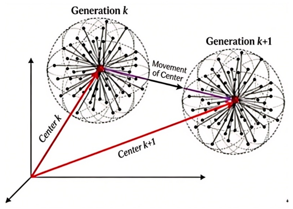
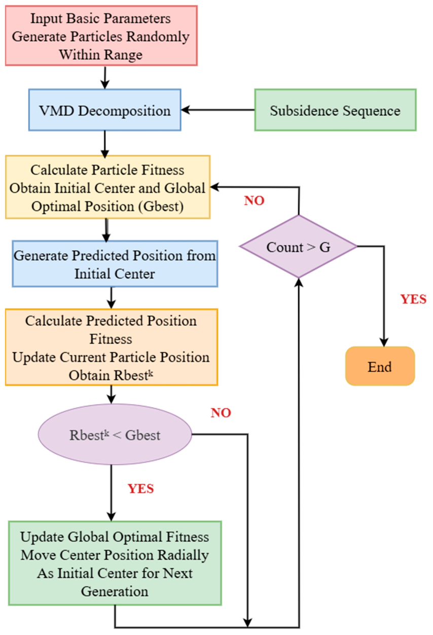
Specifically, IRMO optimizes the center position updating mechanism compared with the original RMO. In each iteration, the search center is updated by combining the global optimal position and local optimal position of particles, which stabilizes the optimization process and effectively avoids local optimal solutions. This optimized center-moving rule is the core improvement in the IRMO algorithm relative to the primitive RMO. The specific optimization principle is illustrated in Figure 1.

(1) Population initialization

The search ranges of parameters $M$ and $\alpha$ are determined first. N initial two-dimensional particles are randomly generated within the ranges according to Equation (8). The fitness function values of the initial generated points are calculated, and the point corresponding to the optimal fitness value is taken as the initial central position Centre¹. The random variable rand(0, 1) adopted in Equation (8) is a universal normalized interval in optimization algorithms. It is used to map random values into the predefined variable search boundary [$\min x_j$, $\max x_j$], so as to generate initial particles within the feasible solution range.

$${\mathbf{X}}^1=\left[\begin{array}{ccccc}{\mathbf{x}}_{\mathrm{1,1}}^1& {\mathbf{x}}_{\mathrm{1,2}}^1& \dots & {\mathbf{x}}_{1,M-1}^1& {\mathbf{x}}_{1,M}^1\\ {\mathbf{x}}_{\mathrm{2,1}}^1& {\mathbf{x}}_{\mathrm{2,2}}^1& \dots & {\mathbf{x}}_{2,M-1}^1& {\mathbf{x}}_{2,M}^1\\ ⋮& ⋮& \ddots & ⋮& ⋮\\ {\mathbf{x}}_{N-\mathrm{1,1}}^1& {\mathbf{x}}_{N-\mathrm{1,2}}^1& \dots & {\mathbf{x}}_{N-1,M-1}^1& {\mathbf{x}}_{N-1,M}^1\\ {\mathbf{x}}_{N,1}^1& {\mathbf{x}}_{N,2}^1& \dots & {\mathbf{x}}_{N,M-1}^1& {\mathbf{x}}_{N,M}^1\end{array}\right]=\left[\begin{array}{c}{\mathbf{x}}_1^1\\ {\mathbf{x}}_2^1\\ ⋮\\ {\mathbf{x}}_{N-1}^1\\ {\mathbf{x}}_N^1\end{array}\right]$$

(7)

$$x_{i,j}^1=\min x_j+\mathrm{r}(\mathrm{0,1})(\max x_j-\min x_j)$$

(8)

(2) Generate a new generation of particles

N new position points $Y_i^k$ are randomly generated around the initial central point as the pre-positions. The pre-position of the k-th generation can be obtained by Equation (9). $w^k$ is defined as a coefficient that decreases with the number of iterations, which enables the solution space to gradually shrink to a single point during the solution process. $w^k$ is calculated by Equation (10), where G is the preset maximum number of iterations, and k is the current generation number. The random variable rand$(-{\displaystyle \frac{1}{2}},{\displaystyle \frac{1}{2}})$ in Equation (9) is designed for symmetric disturbance around the search centre. This positive–negative symmetrical interval ensures uniform radial diffusion of particles on both sides of the central position, and avoids unbalanced directional deviation during the optimization process.

$${\mathit{y}}_{i,j}^k=(\mathrm{r}(-{\displaystyle \frac{1}{2}},{\displaystyle \frac{1}{2}}))(max{\mathit{x}}_j-min{\mathit{x}}_j){\mathit{w}}^k+centr{e}_j^k$$

(9)

$$w^k=1-{\displaystyle \frac{k}{G}}$$

(10)

$${\mathbf{Y}}^k=\left[\begin{array}{ccccc}{\mathrm{y}}_{\mathrm{1,1}}^k& {\mathrm{y}}_{\mathrm{1,2}}^k& \dots & {\mathrm{y}}_{1,M-1}^k& {\mathrm{y}}_{1,M}^k\\ {\mathrm{y}}_{\mathrm{2,1}}^k& {\mathrm{y}}_{\mathrm{2,2}}^k& \dots & {\mathrm{y}}_{2,M-1}^k& {\mathrm{y}}_{2,M}^k\\ ⋮& ⋮& \ddots & ⋮& ⋮\\ {\mathrm{y}}_{N-\mathrm{1,1}}^k& {\mathrm{y}}_{N-\mathrm{1,2}}^k& \dots & {\mathrm{y}}_{N-1,M-1}^k& {\mathrm{y}}_{N-1,M}^k\\ {\mathrm{y}}_{N,1}^k& {\mathrm{y}}_{N,2}^k& \dots & {\mathrm{y}}_{N,M-1}^k& {\mathrm{y}}_{N,M}^k\end{array}\right]=\left[\begin{array}{c}{\mathrm{y}}_1^k\\ {\mathrm{y}}_2^k\\ ⋮\\ {\mathrm{y}}_{N-1}^k\\ {\mathrm{y}}_N^k\end{array}\right]$$

(11)

In the initial stage of iteration, the inertia weight $w^k$ is relatively large, which may cause the search space to exceed the preset range, leading some variables to go beyond the lower bound min x_j or the upper bound max x_j. Therefore, it is necessary to adjust the search space and regenerate the particle ${\mathrm{y}}_{\mathrm{i},\mathrm{j}}^{\mathrm{k}}$ to ensure that all particles are within the preset range [min x_j, max x_j].

$$\{\begin{array}{c}{y}_{i,j}^k=\min x_j+rand(\mathrm{0,1})(\max x_j-\min x_j)w^k,{Centre}_j^{k-1}-{\displaystyle \frac{V_j^k}{2}}<\min x_j\\ y_{i,j}^k=\max x_j-rand(\mathrm{0,1})(\max x_j-\min x_j)w^k,{Centre}_j^{k-1}+{\displaystyle \frac{V_j^k}{2}}>\max x_j\end{array}$$

(12)

(3) Update the central location

The function values $f_i(Y^k)$ of the newly generated pre-positions are calculated and compared with the function values $f_i(X^{k-1})$ of the previous generation. The function value of the i-th point in the current generation is computed according to Equation (13). After updating $f_i(X^k)$, the point corresponding to the minimum value in $f_i(X^k)$ is selected as the optimal position of the current generation, $Rbes{t}^k$. If the current generation optimal position outperforms the global optimal position, the global optimal position $Gbes{t}^k$ is also updated.

$$f_i(X^k)=\min \left\{f_i(Y^k),f_i(X^{k-1})\right\}$$

(13)

The new center position is generated by Equation (14), which is influenced by both the current optimal position and the global optimal position, causing the center position to gradually converge toward the optimal solution. Compared with the original radial movement optimization (RMO) algorithm, the improved IRMO algorithm adopts a more stable center updating mechanism and retains only the optimal solution in each iteration, which effectively improves search stability and avoids unstable results. This improvement makes IRMO more suitable for optimizing VMD parameters for nonlinear, non-stationary, and noisy GNSS settlement time series.

$$Centr{e}^{k+1}=Centr{e}^k+0.4(Gbes{t}^k-Centr{e}^k)+0.5(Rbes{t}^k-Centr{e}^k)$$

(14)

(4) Iterative search

Repeat steps (2) and (3) until the algorithm reaches the final iteration $Gbest$, yielding the desired solution vector with corresponding values representing the optimal parameters.

GNSS monitoring time series of goaf surface settlement present three typical characteristics: strong nonlinearity induced by the coupled effects of geological conditions, mining advancement, and meteorological factors; non-stationarity with distinct evolutionary stages including initial subsidence, active subsidence, and attenuation subsidence; and complex noise contamination caused by multipath interference, ionospheric variation, and instrument observation errors. These inherent characteristics make it difficult to determine the optimal mode number $M$ and penalty factor α of VMD by empirical selection or traditional optimization algorithms, which easily leads to mode aliasing, over-decomposition, or under-decomposition.

IRMO possesses unique optimization mechanisms that are inherently suitable for VMD parameter optimization of nonlinear, non-stationary, and noisy GNSS sequences.

First, IRMO updates the search center by integrating both global optimum and current-generation optimum information [40], which enables adaptive capture of the nonlinear evolution trend in settlement time series and avoids the premature convergence defect of traditional algorithms in nonlinear solution spaces.

Second, IRMO retains only the optimal solution in each iteration and progressively narrows the radial search range via a linearly decreasing coefficient Equation (10). Applied within each settlement stage where the signal characteristics are relatively stationary, this mechanism achieves efficient convergence to stage-specific optimal VMD parameters, thereby avoiding the over-decomposition or mode aliasing that would result from applying uniform parameters across the entire non-stationary sequence.

Third, the symmetric radial disturbance strategy of IRMO maintains stable global exploration capability, which can effectively suppress the interference of random GNSS noise on parameter optimization, reduce the dispersion of repeated search results, and ensure the stability and physical interpretability of decomposed IMF components.

2.1.3. IRMO-VMD Combined Algorithm

Variational Mode Decomposition (VMD) has achieved remarkable performance in noise reduction and feature extraction and has been applied by scholars to the processing of GNSS monitoring sequences [19,43]. However, the values of the decomposition mode number $M$ and the penalty factor $\alpha$ have a significant impact on the decomposition results. If $M$ is too small, the low-frequency components are prone to overlap with high-frequency components, which is not conducive to the identification of intrinsic mode functions (IMFs); if $M$ is too large, it will lead to mode over-decomposition. For the penalty factor $\alpha$, an excessively small value will cause a large amount of noise in the decomposed modes, while an excessively large value will result in the key parts of the signal or spectrum being split into different components [38]. To find the optimal VMD parameters, this paper introduces the Improved Radial Movement Optimization (IRMO) algorithm to optimize the VMD parameters. The IRMO algorithm is a global optimization algorithm that can quickly solve the optimal value of nonlinear multi-objective functions. In practical engineering applications without reference data and prior experience, it is hard to select appropriate values of mode number M and penalty factor α for VMD. To solve this problem, the IRMO algorithm is used in this paper to adaptively optimize these two parameters. The optimal combination of M and α can be automatically determined according to the inherent characteristics of the original monitoring signal, without relying on any external reference information or manual empirical selection. Therefore, this paper uses the IRMO algorithm to find the optimal parameter combination for VMD. The specific flow of the IRMO-VMD algorithm is shown in Figure 2.

2.1.4. Design of Fitness Function for IRMO-VMD Algorithm

To objectively evaluate the parameter optimization performance of the improved radial moving optimization algorithm (IRMO) on variational mode decomposition (VMD), this study adopts minimum kurtosis value as the fitness function for the IRMO-VMD algorithm. Kurtosis, a statistical measure describing the steepness of signal probability distributions and tail characteristics, exhibits a direct correlation with signal stationarity: higher kurtosis values indicate more concentrated probability distributions prone to abrupt changes and violent fluctuations, while lower values signify more uniform and continuous distributions with superior stability. Given the objective of decomposing noisy non-stationary GNSS subsidence sequences into stable, frequency-concentrated intrinsic mode functions (IMFs) to meet temporal modeling requirements for subsequent GRU models, the minimum kurtosis value serves as the IRMO algorithm’s fitness metric. Through optimization processes, the algorithm minimizes the total kurtosis values of all IMF components post-VMD, thereby achieving stable subsidence sequence decomposition. The specific calculation formula for the minimum kurtosis value is presented in Equation (15):

$$\{\begin{array}{c}F(X)=\min ({\displaystyle \frac{{\mu }_1}{{\sigma }_1^4}},{\displaystyle \frac{{\mu }_2}{{\sigma }_2^4}},{\displaystyle \frac{{\mu }_3}{{\sigma }_3^4}}\dots {\displaystyle \frac{{\mu }_k}{{\sigma }_k^4}})\\ {\sigma }_k=\sqrt{{\displaystyle \frac{1}{N-1}}{\sum }_i^N{(u_i^k-{\bar{u}}^k)}^2}\\ {\mu }_k={\displaystyle \frac{1}{n}}{\sum }_i^N{(u_i^k-{\bar{u}}^k)}^4\end{array}$$

(15)

where $u_i^k$ is the decomposed sequence of the k-th mode; ${\overline{u}}^k$ is the mean value of the decomposed sequence of the k-th mode; ${\mu }_k$ is the fourth-order central moment of the sequence; and ${\sigma }_k$ is the standard deviation of the sequence.

The selection of minimum kurtosis as the fitness function is further supported by established signal processing theory [44]. As demonstrated, kurtosis remains robust to additive Gaussian noise while exhibiting high sensitivity to the peakedness and non-stationary characteristics of time series. This property is particularly suited to GNSS subsidence monitoring data, which is inherently non-stationary and often contaminated by complex measurement noise. By minimizing the overall kurtosis of all IMF components during VMD, the IRMO algorithm effectively drives the decomposition toward physically meaningful, frequency-concentrated modes, laying a solid foundation for subsequent GRU modeling.

2.2. Construction of the IRMO-VMD-GRU Combined Model and Performance Evaluation Indicators

2.2.1. Gated Recurrent Unit (GRU)

The Gated Recurrent Unit (GRU) is an improved variant of the Recurrent Neural Network (RNN), originally designed to overcome the gradient vanishing and gradient explosion problems that are prevalent in traditional RNNs when processing long time-series data. By leveraging a gating mechanism to dynamically regulate the information transmission process, GRU can efficiently capture long-term correlation features in complex time-series dependency scenarios, providing a more robust solution for the modeling and analysis of sequence data.

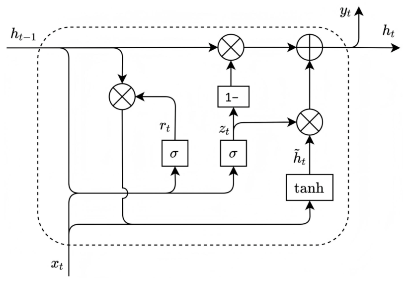
The network architecture of the Gated Recurrent Unit (GRU) (Figure 3) is relatively concise, with its core lying in the internal state cell—a unit capable of maintaining long-term states and temporal memory, which provides fundamental support for long-sequence modeling. The key of the GRU neural network lies in the introduction of two core gating mechanisms: the update gate and the reset gate. By dynamically regulating the retention and discard of information, the two gates achieve accurate screening of key correlation information in time-series data. Among them, the outputs of the update gate and reset gate are denoted as $z_t$ and $r_t$, respectively, whose calculation processes are shown in Equations (16) and (17):

$$z_t=\sigma (W_z\cdot \left[h_{t-1},x_t\right])$$

(16)

$$r_t=\sigma (W_r\cdot \left[h_{t-1},x_t\right])$$

(17)

where $W_z$ and $W_r$ are the weight matrices of the update gate and reset gate, respectively; $h_{t-1}$ denotes the hidden state from the previous time step; $x_t$ represents the input at the current time step; and $\sigma$ is the sigmoid activation function that compresses output values between 0 and 1.

In the GRU architecture, the core role of the update gate and reset gate is to regulate the flow of information. Here, the sigmoid function is adopted as the activation function for both the update gate and the reset gate, a design derived from the original GRU model proposed by Cho et al. [45]. Mathematically, the gating mechanism can be interpreted as a “retention ratio”—the gate output must be constrained within the range of (0, 1) to accurately represent the proportion of information to be retained or discarded. As explicitly noted by Cho et al. [45], “it is crucial to use this new unit with gating units,” and meaningful results cannot be obtained using only the tanh unit without any gating mechanism.

By utilizing the outputs of the update gate and reset gate, we can compute the candidate hidden state ${\tilde{h}}_t$ and the final time state $h_t$ at the current time step.

$${\tilde{h}}_i=\tan h(W\cdot \left[r_i{h}_{-1},x_i\right])$$

(18)

$$h_t=(1-z_t)\ast h_{t-1}+z_t\ast {\tilde{h}}_t$$

(19)

where $W$ is the weight matrix of candidate hidden states; $r_t{h}_{t-1}$ represents the element-wise product of the reset gate output and the previous hidden state; $tanh$ is the hyperbolic tangent activation function used to introduce nonlinearity; $(1-z_t)\ast h_{t-1}$ indicates the proportion of the previous hidden state retained in the current hidden state; and $z_t\ast {\tilde{h}}_t$ denotes the newly added information from the candidate hidden states.

Through this approach, GRU can effectively regulate information flow, enabling the model to better handle dependencies in long sequence data.

2.2.2. Design of IRMO-VMD-GRU Combined Model

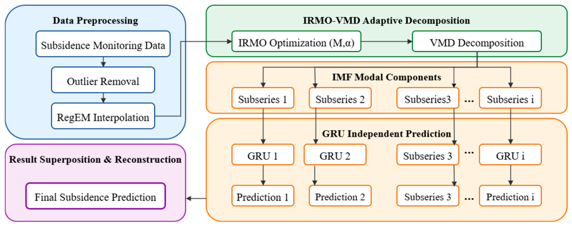
This study proposes an integrated forecasting model (IRMO-VMD-GRU) based on an improved radial moving optimization algorithm (IRMO), variational mode decomposition (VMD), and gated recurrent unit (GRU). The model employs IRMO-VMD to adaptively decompose surface subsidence sequences into a set of intrinsic mode function (IMF) sequences with distinct characteristics. The IRMO algorithm optimizes key VMD hyperparameters (mode count and penalty factor). Subsequently, the GRU neural network independently trains each IMF sequence to generate single-modal predictions, with final forecast values reconstructed from modal result integration. The implementation steps are illustrated in Figure 4.

Step 1: Perform outlier identification and removal on the surface subsidence sequence, employ the regularization expectation maximization (RegEM) interpolation technique to fill missing data, and construct a complete dataset; then divide the dataset into Training Set and Testing Set according to predefined proportions to provide standardized input for subsequent modeling.

Step 2: Input the Training Set into the IRMO-VMD algorithm. IRMO performs global optimization on two core hyperparameters of VMD (mode decomposition number $M$ and penalty factor $\alpha$), using minimum kurtosis as the fitness function to ensure stability of the decomposed IMF. This yields multiple modal components ($u_1$, $u_2$, $u_3$ … $u_i$). The Testing Set then employs the same optimal hyperparameters from the Training Set for decomposition, ensuring consistency in modal features.

Step 3: The modal components obtained from decomposing the Training Set and Testing Set using the IRMO-VMD algorithm are separately fed into the gated recurrent unit (GRU) model for independent training.

Step 4: Perform stacking reconstruction on the prediction results of each modal component in the Testing Set to obtain the final land subsidence prediction results for the IRMO-VMD-GRU model.

2.2.3. Performance Evaluation Indicators

To comprehensively evaluate the predictive performance of the proposed model, this study selects four metrics: mean absolute error ($Mean Absolute Error, MAE$), root mean square error ($Root Mean Square Error, RMSE$), mean absolute percentage error ($Mean Absolute Percentage Error, MAPE$), and correlation coefficient (${Coefficient of Determination, R}^2$) to assess the model’s overall performance.

$$MAE={\displaystyle \frac{1}{n}}{\displaystyle {\sum }_{i=1}^n}\left|y_i-{\widehat{y}}_i\right|,$$

(20)

$$RMSE=\sqrt{{\displaystyle \frac{1}{n}}{\sum }_{i=1}^n{(y_i-{\widehat{y}}_i)}^2}$$

(21)

$$MAPE={\displaystyle \frac{100\%}{n}}{\displaystyle \sum _{i=1}^n}\left|{\displaystyle \frac{y_i-{\widehat{y}}_i}{y_i}}\right|$$

(22)

$$R^2=1-{\displaystyle \frac{{\sum }_{i=1}^n{({\widehat{y}}_i-y_i)}^2}{{\sum }_{i=1}^n{(y_i-\bar{y})}^2}}$$

(23)

In the above equations, $y_i$ represents the measured (observed) value of the i-th sample, ${\widehat{y}}_i$ is the corresponding predicted value obtained by the model, $\bar{y}$ is the mean of all measured values, and n denotes the total number of samples. $MAE$ reflects the average absolute error between predicted and measured values, $RMSE$ is sensitive to large prediction errors and evaluates the overall deviation, $MAPE$ measures the relative error as a percentage, and $R^2$ quantifies the proportion of variance in the measured values explained by the model, with a value closer to 1 indicating a better fitting performance.

3. Results

3.1. Study Area and Preprocessing of Settlement Monitoring Data

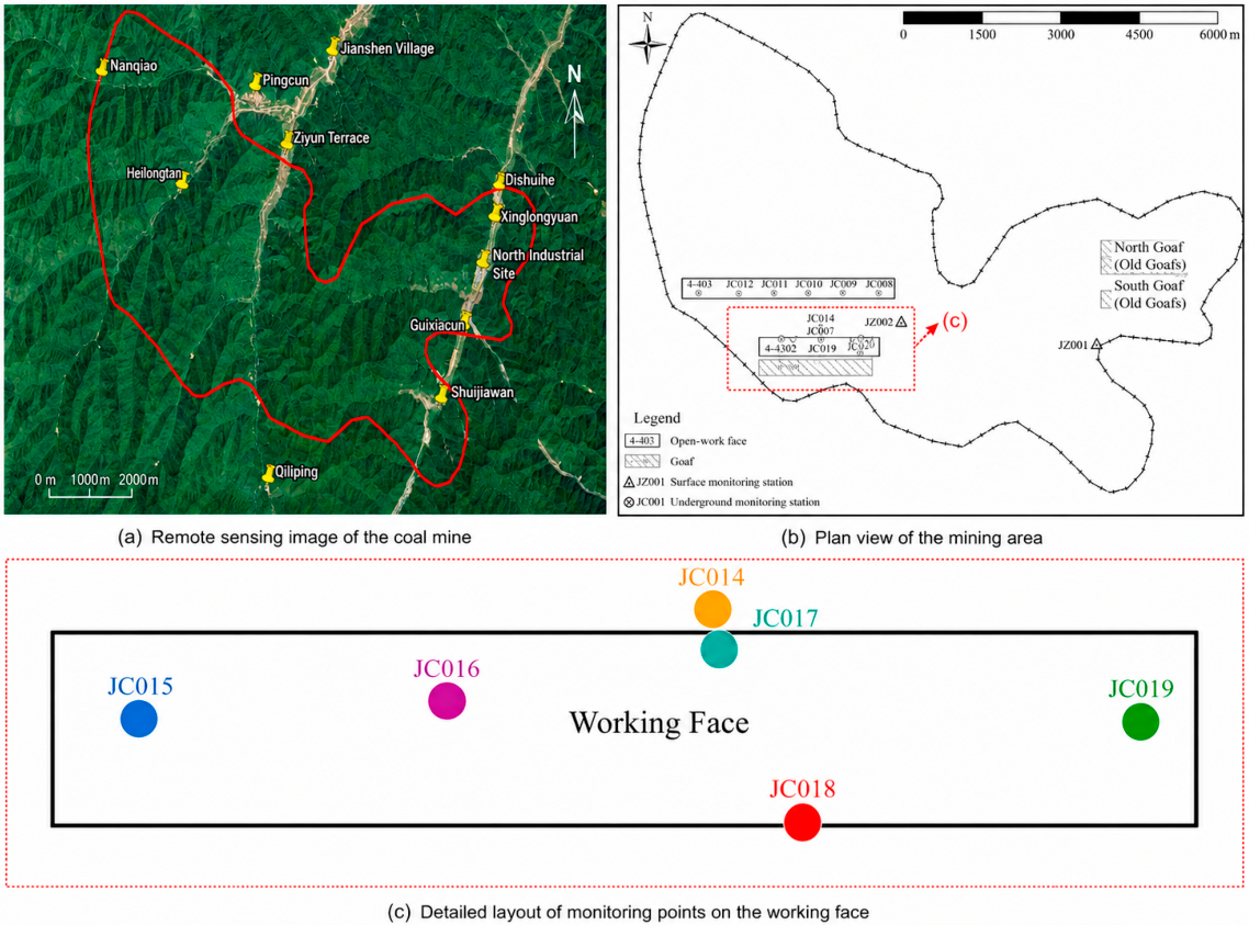
The study area is the Jianbei Coal Mine in Huangling County, Shaanxi Province, China. The mine is administratively under the jurisdiction of Yan’an City, with geographical coordinates of 108°48′15″–108°57′00″ E and 35°23′15″–35°29′00″ N. The mining rights area spans 4–9 km north–south and approximately 13.5 km east–west, covering a total area of 48.1524 km². The subsidence monitoring data were collected using GNSS sensors at the 4-2302 working face, which commenced mining operations in 2022. During the mining phase, six GNSS monitoring stations were strategically positioned above the working face to track ground deformation caused by mining activities and assess its progression. The spatial distribution and exact locations of these GNSS stations are illustrated in Figure 5, while detailed monitoring point specifications are presented in

Table 1. Information of GNSS monitoring points.

Monitoring Point	Longitude	Latitude	Time Span	Missing Rate (%)
JC014	108.859085	35.421851	2022.12–2024.6	10.7
JC015	108.848772	35.419444	2022.12–2024.6	23.9
JC016	108.854683	35.419899	2022.12–2024.6	33.5
JC017	108.859287	35.420626	2022.12–2024.6	4.9
JC018	108.86658	35.419498	2022.12–2024.6	4.9
JC019	108.860174	35.417897	2022.12–2024.6	5.3

.

GNSS monitoring stations upload data every 10 min, containing instantaneous coordinates in the X, Y, and Z directions. Since surface settlement values correlate with Z-direction coordinate changes, the initial coordinates are determined by calculating the average Z-direction coordinates of each monitoring point on the first day. Subsequent settlement values are then computed by measuring the difference between each day’s average coordinates and the initial value.

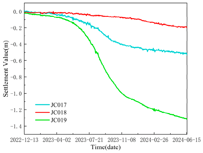
Due to signal interference, equipment malfunctions, and other factors, data from all six monitoring stations exhibit varying degrees of missing values. Stations JC014, JC015, and JC016 demonstrate notably higher missing rates with significant temporal gaps in data, rendering them inadequate for accurately reflecting actual surface subsidence trends. Consequently, this study selects monitoring data from JC017, JC018, and JC019 stations located on the working face. These stations provide more comprehensive subsidence measurements that reliably capture ground subsidence patterns during mining operations.

For datasets with missing sedimentation sequences, this study employs the Regularized Expectation Maximum (RegEM) algorithm for interpolation. The RegEM algorithm utilizes incomplete datasets by iteratively estimating mean values and covariance matrices through regression analysis, then applying these parameters to interpolate missing values [46].

The specific steps of the RegEM algorithm are as follows:

(1) Collect monitoring data from p monitoring points over n days to construct an n × p observation matrix X containing missing values. The element xi,j in matrix X represents the observed value at monitoring point j (j = 1, 2, 3, …, p) at time i (i = 1, 2, 3, …, n). For the observed data at time i, the non-missing data are grouped into a row vector ${\mathrm{Z}}_a$ (where a is the number of non-missing data), with its mean and covariance matrix denoted as ${\mu }_a$ and ${\sum }_{aa}$, respectively. For the missing data at this time point, initial values are assigned using column means, simple interpolation, or random filling to form a row vector ${\mathrm{Z}}_m$ (where m is the number of missing data), with its mean and covariance matrix denoted as ${\mu }_m$ and ${\sum }_{mm}$. Additionally, the cross-covariance matrix between ${\mathrm{Z}}_a$ and ${\mathrm{Z}}_m$ is denoted as ${\sum }_{am}$.

(2) Based on the covariance matrix ${\sum }_{aa}$ and the cross-covariance matrix ${\sum }_{am}$, the regression coefficient estimates B for all time points containing missing data in matrix X are solved through regularized maximum likelihood estimation. The calculation formula is as follows:

$$\widehat{B}={({\Sigma }_{aa}+h^{2}D)}^{-1}{\Sigma }_{am}$$

(24)

where h is the regularization parameter determined by generalized cross-validation (GCV); D is the diagonal matrix of ${\sum }_a$.

The estimated values of the missing data, ${\widehat{\mathrm{Z}}}_m$, can be calculated based on the mean of missing data ${\mu }_m$, the non-missing data vector ${\mathrm{Z}}_a$, the mean of non-missing data ${\mu }_a$, and the estimated regression coefficients $\widehat{\mathrm{B}}$. The calculation formula is as follows:

$${\widehat{Z}}_m={\mu }_m+(Z_a-{\mu }_a)\widehat{B}+e$$

(25)

where e is a 1 × m dimensional random vector with a mean of 0 and a covariance matrix C. The formula for calculating C is as follows:

$$C={\Sigma }_m-{\Sigma }_{am}^{\prime }{({\Sigma }_a+h^{2}D)}^{-1}{\Sigma }_{am}$$

(26)

(3) Using the estimated missing data values ${\widehat{\mathrm{Z}}}_m$ obtained in step (2), update the mean ${\mu }_m$ and covariance ${\sum }_{\mathrm{m}\mathrm{m}}$, and recalculate the cross-covariance matrix ${\sum }_{am}$ between ${\mathrm{Z}}_a$ and ${\widehat{\mathrm{Z}}}_m$.

(4) Repeat steps (2) and (3) iteratively until the changes in both the mean ${\mu }_m$ and the covariance matrix ${\sum }_{mm}$ of ${\mathrm{Z}}_m$ converge to a specified threshold, and output the final imputed complete settlement series.

Independent of specific mathematical models or external prior knowledge, this approach leverages regularization techniques to maintain data stability and accuracy while mitigating biases caused by missing values. Figure 6 presents the interpolated results obtained using the RegEM algorithm.

3.2. Performance Comparison Analysis of IRMO-VMD Algorithm

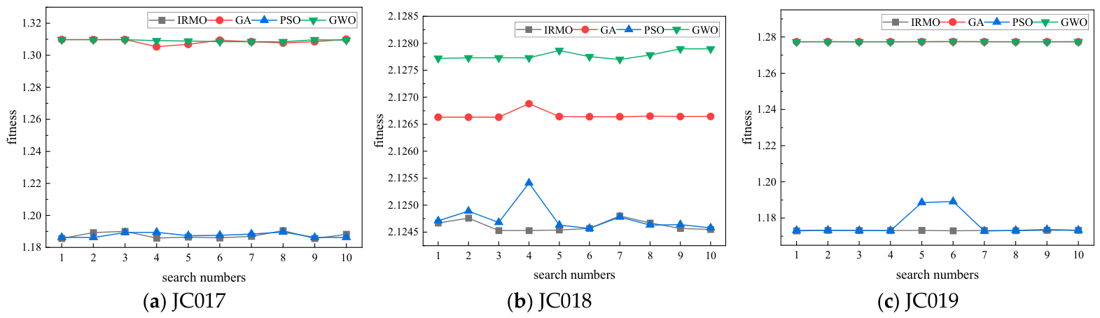
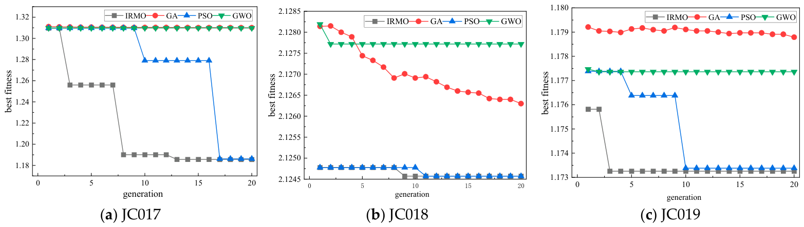
To verify the superiority of the IRMO algorithm in VMD parameter optimization, the Genetic Algorithm (GA), Particle Swarm Optimization (PSO) algorithm, and Grey Wolf Optimizer (GWO) were selected for comparison with the IRMO algorithm. The settlement monitoring data at three points, JC017, JC018, and JC019, were used as input data. The population size of the algorithms was set to 50, the maximum number of iterations was set to 20, the range of parameter M was set to [1, 10], and the range of $\alpha$ was set to [10, 2500]. A smaller value of mode number M easily causes modal aliasing, while an excessively large M leads to over-decomposition; the penalty factor $\alpha$ affects decomposition accuracy by restricting the bandwidth of each decomposed mode [34], and the minimum kurtosis value was selected as the fitness function. The convergence curves of the four optimization algorithms are shown in Figure 7, and the 10 search results are shown in Figure 8. It can be seen from Figure 7 that, compared with the GA and GWO algorithms, the IRMO algorithm has a steeper convergence curve, and the finally converged optimal fitness value (minimum kurtosis value) is lower; compared with the PSO algorithm, the difference in optimal fitness values between the two is negligible, but the IRMO algorithm can quickly approach the optimal value in the early stage of iteration, exhibiting a faster convergence speed. It can be seen from Figure 8 that after 10 independent repeated searches, the dispersion of the IRMO algorithm results is significantly smaller than that of the comparison algorithms, and the output results remain consistently stable, demonstrating higher stability and global search capability. In conclusion, compared with the GA, GWO, and PSO algorithms, the IRMO algorithm not only has faster convergence speed but also higher stability and stronger global search capability in VMD parameter optimization, consistently exhibiting excellent performance.

In conclusion, compared with the GA, GWO, and PSO algorithms, the IRMO algorithm not only has faster convergence speed but also higher stability and stronger global search capability in VMD parameter optimization, consistently exhibiting excellent performance. As reported in Pan et al. [40], IRMO improves the center iteration mechanism on the basis of the original RMO algorithm, retaining only the optimal solution per generation. The convergence curves and multiple repeated search results in Figure 7 and Figure 8 further verify its inherent superiority. In comparison with GA, PSO and GWO, IRMO converges faster in the early iteration stage, and the dispersion of multiple independent search results is much smaller, showing higher robustness and global optimization stability. Therefore, IRMO can stably obtain the optimal combination of VMD mode number and penalty factor, and is more applicable to the decomposition of complex noisy goaf settlement sequences.

3.3. Comparative Analysis of Prediction Performance for IRMO-VMD-GRU Models

3.3.1. IRMO-VMD Sedimentation Sequence Decomposition and Feature Analysis

During mining activities, surface subsidence typically progresses through three distinct phases characterized by different subsidence rates: the initial subsidence phase (v ≤ 1.67 mm/day) with both subsidence volume and rate being relatively low; the active subsidence phase (v > 1.67 mm/day) featuring a higher subsidence rate; and the decaying subsidence phase (v ≤ 1.67 mm/day) where the subsidence rate gradually decreases [47]. Tashman [48] emphasizes that single-test periods are susceptible to subjective time selection biases, resulting in unstable evaluation outcomes; thus, out-of-sample validation should be conducted across multiple testing cycles. Additionally, the test set length should not be shorter than the actual prediction duration, and excessive testing windows should be avoided to prevent over-compression of training data, which could compromise model performance. Accordingly, this study adopts an alternative approach rather than the conventional fixed-proportion division method. Instead, independent testing cycles are established for each subsidence phase, with the final 30 days of each phase selected as test samples—a practice that aligns with out-of-sample evaluation standards for time-series forecasting and meets the practical needs of monthly mine engineering monitoring. Throughout the research, model evaluation is performed using a rolling origin methodology.

The specific time periods for each monitoring site in this article are divided as follows: In the dataset division, the settlement data of the last 30 days of these three stages were taken as the Testing Set, and the settlement data prior to these 30 days were used as the Training Set. The three stages at the JC019 monitoring point were relatively distinct: the initial settlement stage lasted from 13 December 2022 to 12 May 2023, the active settlement stage spanned from 12 May 2023 to 28 November 2023, and the decaying settlement stage commenced after 28 November 2023. Due to the relatively small settlement magnitude at the JC018 monitoring point, it was impossible to identify the three settlement stages; therefore, the time division of the three stages at the JC019 point was adopted for JC018. For the JC017 monitoring point, the initial settlement stage occurred from 13 December 2022 to 30 June 2023, the active settlement stage was from 30 June 2023 to 8 October 2023, and the decaying settlement stage followed after 8 October 2023. The division of the Training Set and Testing Set for each monitoring point is presented in

Table 2. Division of Training Set and Testing Set for each monitoring site.

Monitoring Point	Settlement Stage	Training Set	Testing Set
JC017	Initial Stage	170	30
	Active Stage	270	30
	Decay Stage	521	30
JC018	Initial Stage	121	30
	Active Stage	321	30
	Decay Stage	521	30
JC019	Initial Stage	121	30
	Active Stage	321	30
	Decay Stage	521	30

.

After interpolating the settlement sequences using the RegEM method, the IRMO-VMD algorithm was employed to decompose the three training set settlement sequences, respectively. The same decomposition was performed on their respective testing sets based on the obtained optimal parameters. The number of iterations of the IRMO algorithm was set to 20, the range of parameter M was set to [1, 10], the range of $\alpha$ was set to [10, 2500], and the minimum kurtosis factor was selected as the fitness function. By inputting these parameters into the IRMO-VMD algorithm, the settlement sequences at the three monitoring points were decomposed, and the resulting optimal parameters are presented in

Table 3. Optimal decomposition parameters of IRMO-VMD.

Monitoring Point	Settlement Stage	M	$\mathit{\alpha }$	Minimum Kurtosis
JC017	Initial Stage	8	1822	1.5868
	Active Stage	5	1136	1.5734
	Decay Stage	10	1583	1.1856
JC018	Initial Stage	10	853	2.0040
	Active Stage	9	2353	1.7834
	Decay Stage	10	2438	2.1245
JC019	Initial Stage	10	1675	1.5496
	Active Stage	10	1050	1.5773
	Decay Stage	10	2044	1.1729

.

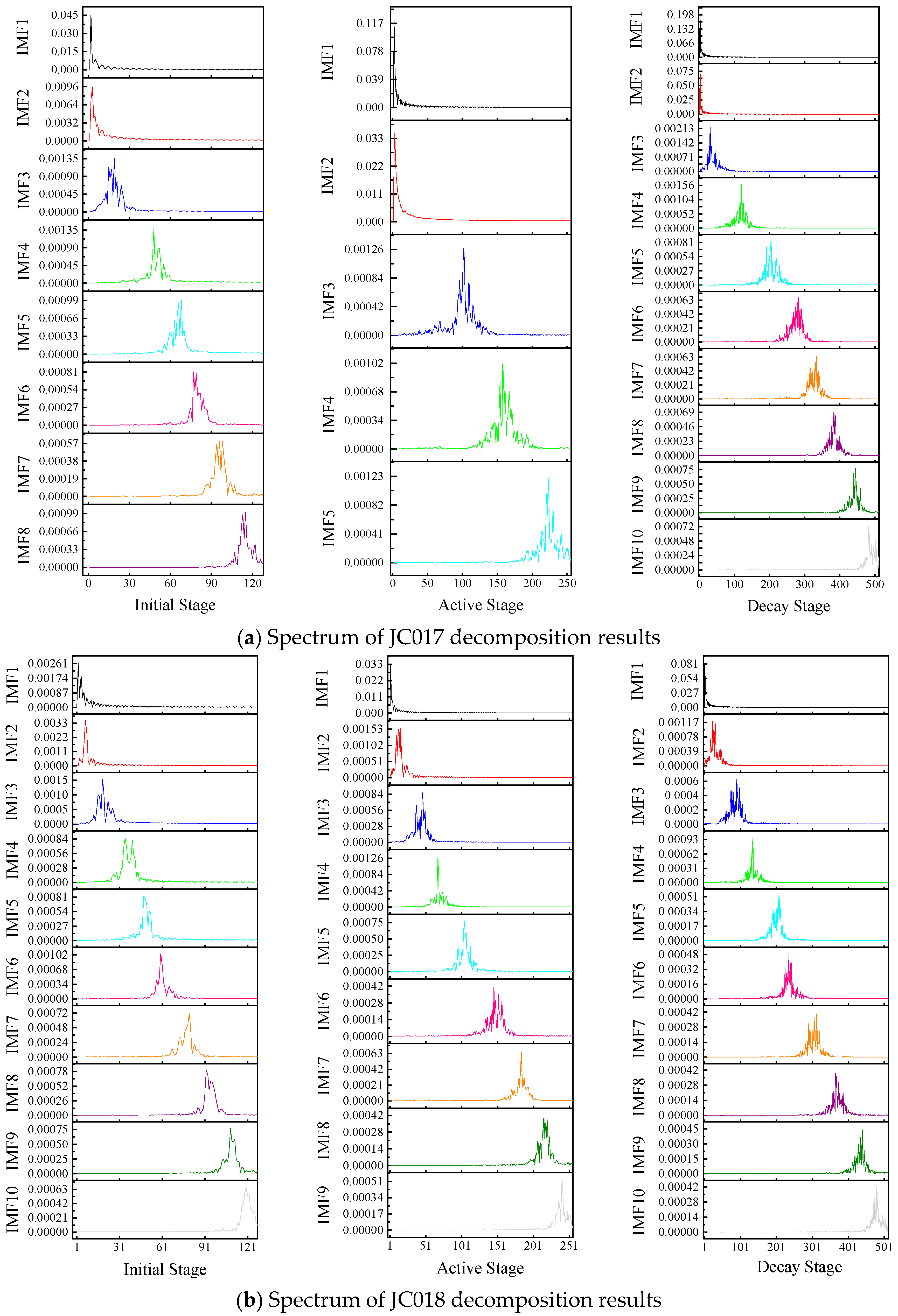
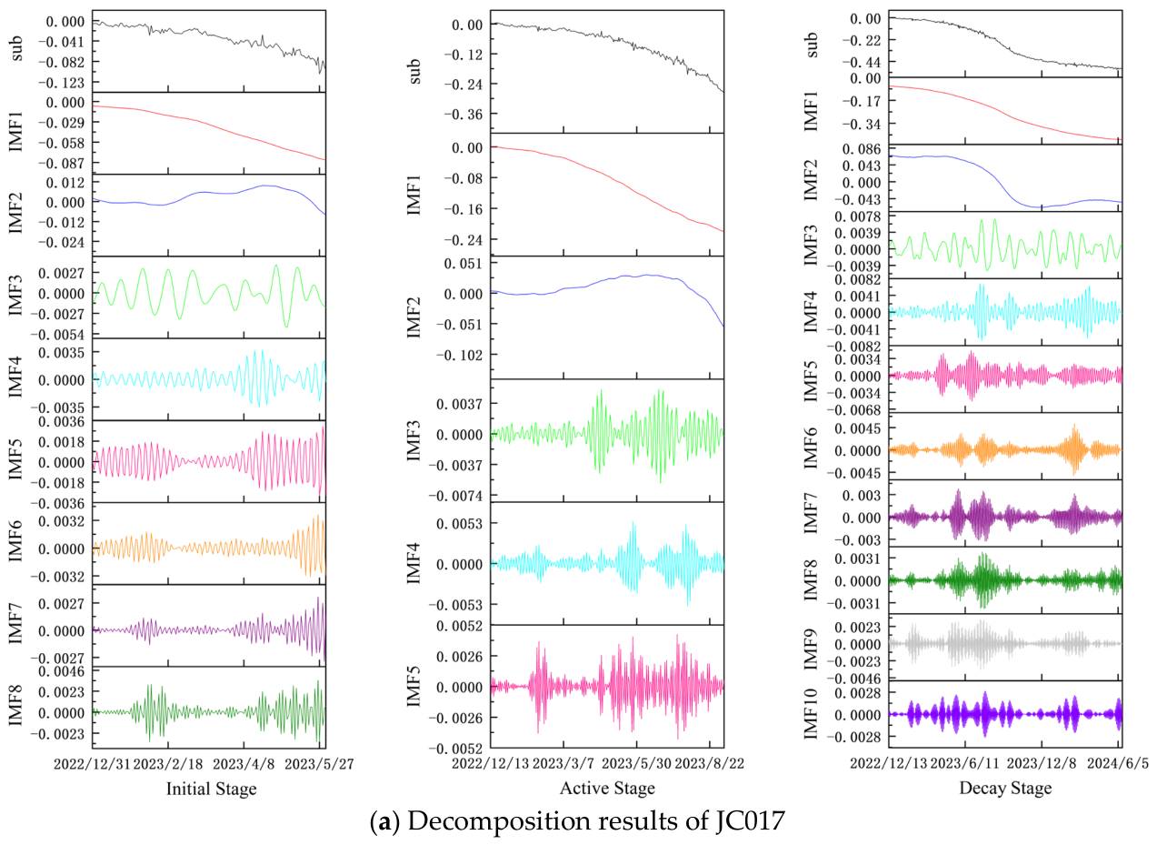
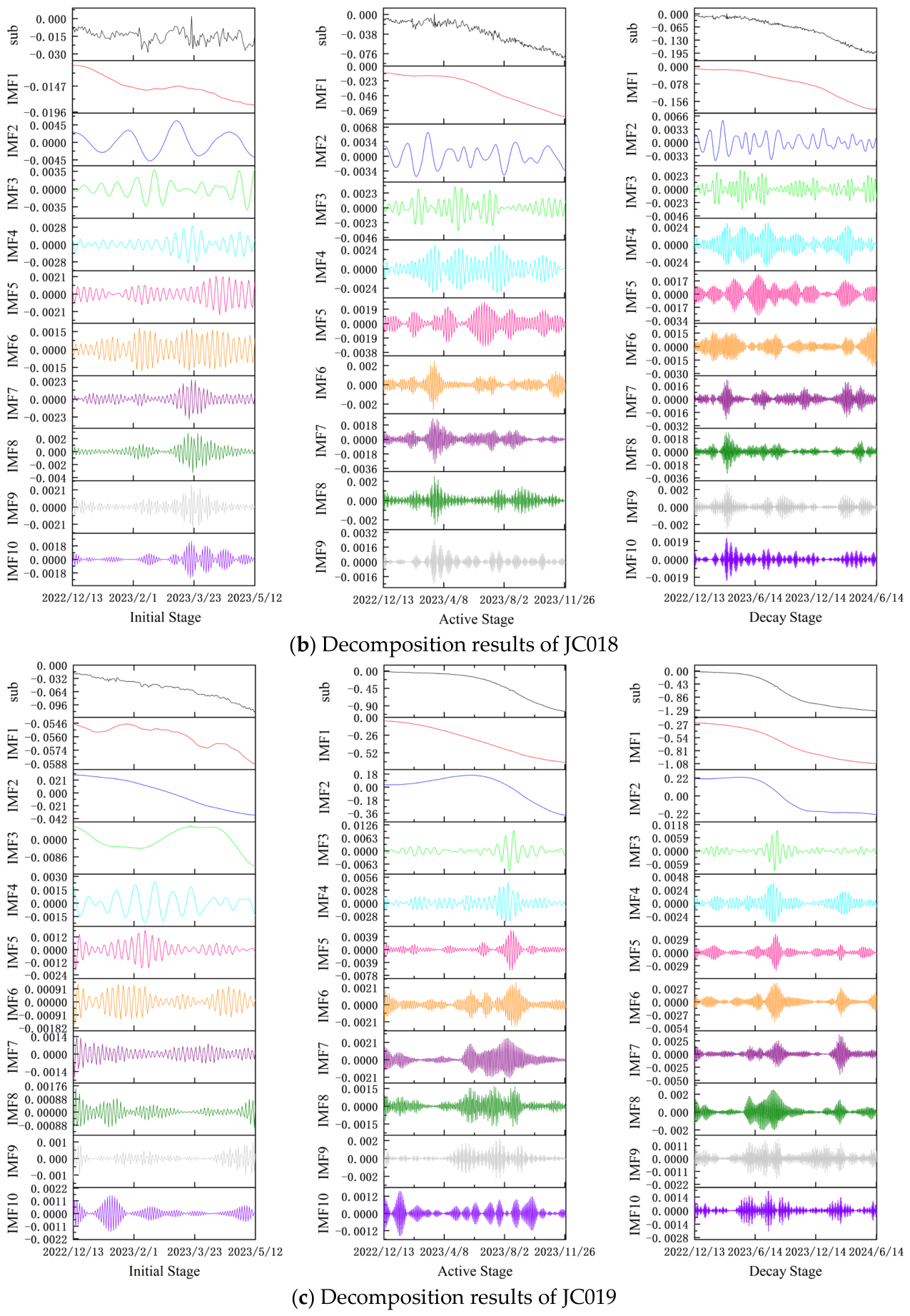
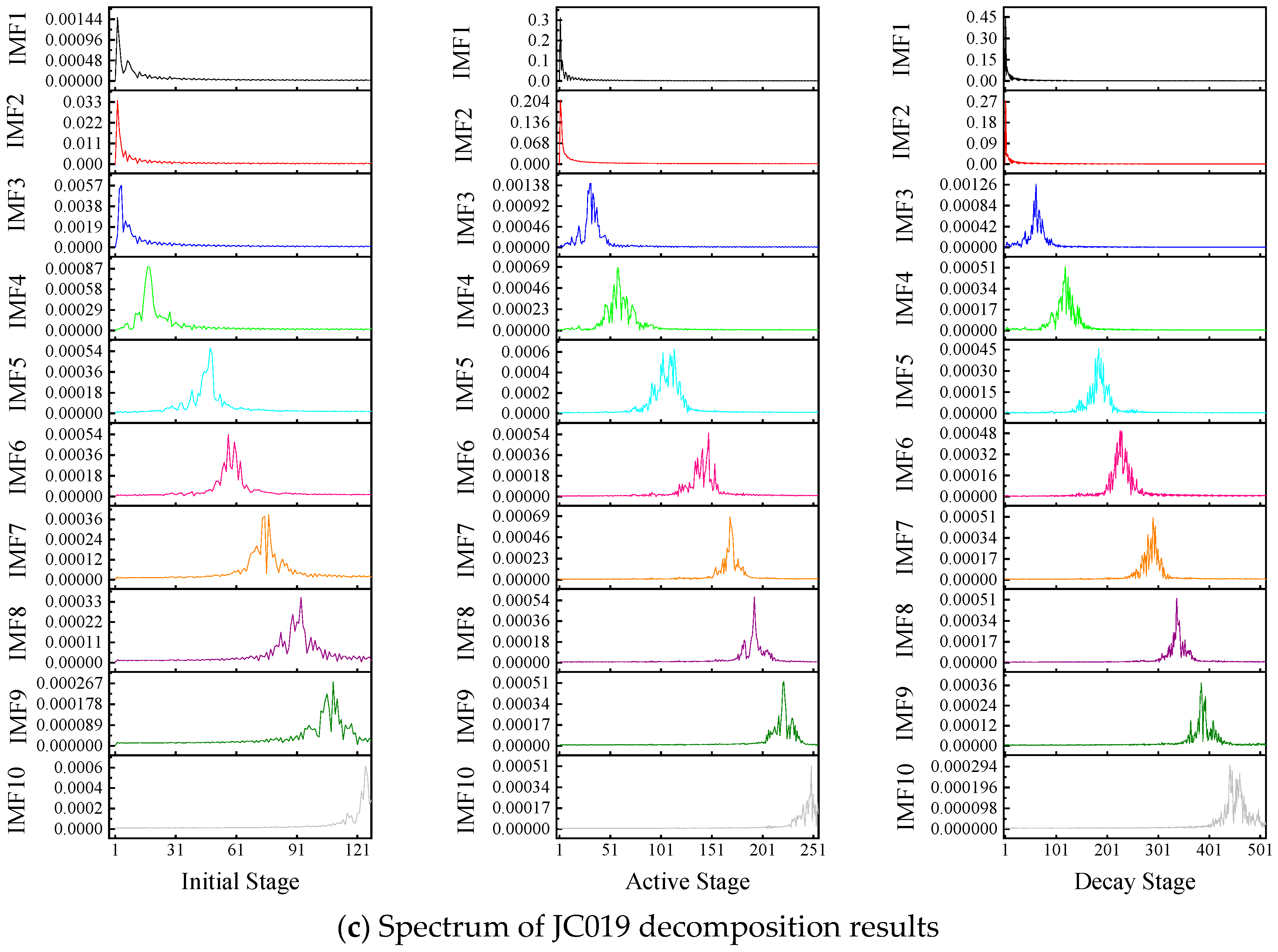
The obtained optimal parameters M and $\alpha$ were input into the VMD to decompose the corresponding settlement sequences, and the decomposition results of the settlement sequences at each monitoring point in different stages are shown in Figure 9. After decomposition by the IRMO-VMD algorithm, the original sequence is decomposed into more regular and stable sub-sequences. The IRMO-VMD effectively extracts the main features of the settlement data and significantly reduces noise interference in the data. Fast Fourier Transform (FFT) was employed to analyze each sub-sequence, and the results are presented in Figure 10. The first two modal components with large amplitudes exhibit significantly consistent periods, indicating that the three monitoring points share a consistent long-term settlement trend, which is consistent with the basic law of surface subsidence in goaf areas. The spectral energy is predominantly concentrated in the first two IMFs within the low-frequency range, consistent with the long-term slow deformation characteristics of goaf settlement. The spectral amplitudes of different modes vary to some extent. The dominant frequency positions are stable across all monitoring points, indicating that the main spectral components share a consistent structure. The above results show that the IRMO-VMD algorithm has certain effectiveness in decomposing the original settlement sequence, can obtain stable and uniform sub-sequences, accurately extract the key features of the monitoring data, and can effectively reduce noise interference at the same time.

3.3.2. IRMO-VMD-GRU Model Sedimentation Prediction

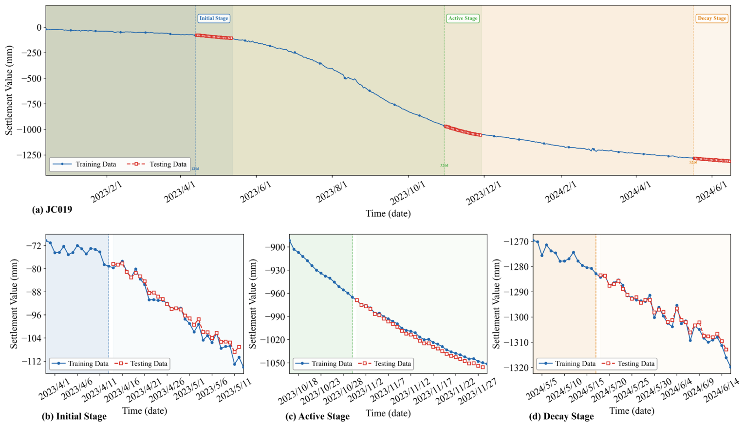
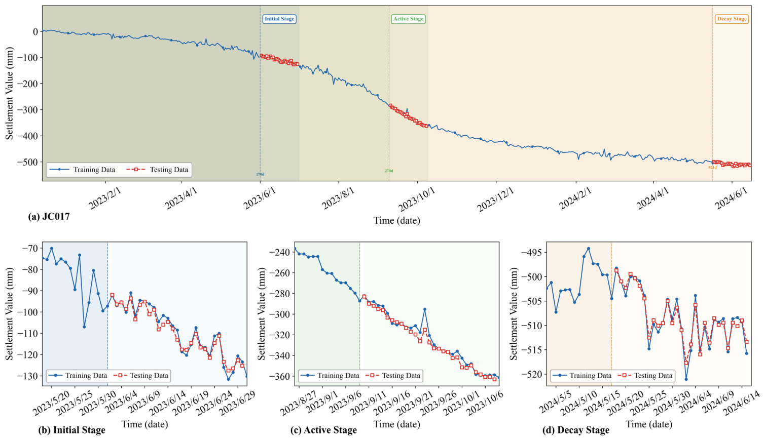
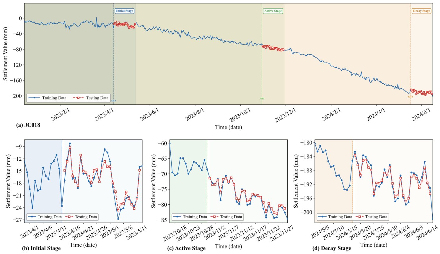
After completing the sedimentation sequence decomposition, the decomposed modal components from both the Training Set and Testing Set are fed into the GRU model for training. The predicted results are then reconstructed to obtain final sedimentation values. The GRU neural network features a single input dimension, 100 hidden units, a maximum training iteration limit of 150, an initial learning rate of 0.005, and a regularization parameter of 0.0001. The time step (time_steps) is set to 11, meaning the sedimentation data from the previous 11 days is used to predict the 12th day’s sedimentation. These hyperparameters were determined through experimental tuning, and a sensitivity analysis confirmed that the model performance was insensitive to hyperparameter choices within reasonable ranges. Given the temporal nature of surface sedimentation data, the training process maintains the original sequence order without randomization. All experiments were conducted on a workstation equipped with an Intel Core i9-13900H processor (14 cores, 16 GB RAM) running Python 3.13 with PyTorch 2.10.0. The full experimental pipeline was completed within approximately 3.8 h, indicating acceptable computational cost for practical deployment. The prediction results are presented in Figure 11, Figure 12 and Figure 13.

3.3.3. Comparison of Multiple Prediction Results and Validity Verification

To verify the superiority of the IRMO-VMD-GRU combined model, a single GRU model and a VMD-GRU model were used as comparison models and compared with the IRMO-VMD-GRU combined model. In both comparison models, the parameters of the GRU part, the Training Set and the Testing Set were consistent with the IRMO-VMD-GRU combined model. In the VMD-GRU model, the decomposition mode number M of VMD was set to 6, and the penalty factor $\alpha$ was set to 1200. The performance evaluation results of the three models are shown in

Table 4. Comparison of prediction error indexes of different models.

Monitoring Point	Model	Settlement Stage	MAE (mm)	RMSE (mm)	MAPE (%)	R2
JC017	GRU	Initial Stage	4.986	6.222	4.72	0.713
		Active Stage	4.579	6.652	1.43	0.929
		Decay Stage	4.880	6.491	0.95	0.353
	VMD-GRU	Initial Stage	3.458	4.419	3.05	0.855
		Active Stage	4.016	5.650	1.27	0.949
		Decay Stage	1.966	2.557	0.38	0.787
	IRMO-VMD-GRU	Initial Stage	1.911	2.336	1.76	0.959
		Active Stage	3.750	5.390	1.19	0.953
		Decay Stage	1.000	1.260	0.20	0.948
JC018	GRU	Initial Stage	3.550	4.500	21.92	0.1367
		Active Stage	2.520	3.313	3.24	0.524
		Decay Stage	4.133	4.766	2.19	−0.281
	VMD-GRU	Initial Stage	1.907	2.378	12.73	0.759
		Active Stage	0.853	1.160	1.07	0.932
		Decay Stage	1.445	1.716	0.76	0.835
	IRMO-VMD-GRU	Initial Stage	1.240	1.570	7.88	0.895
		Active Stage	0.771	1.036	0.97	0.946
		Decay Stage	0.955	1.045	0.50	0.939
JC019	GRU	Initial Stage	5.131	5.799	5.31	0.691
		Active Stage	7.598	7.756	0.75	0.912
		Decay Stage	2.067	2.716	0.16	0.904
	VMD-GRU	Initial Stage	1.551	1.893	1.624	0.968
		Active Stage	5.628	5.947	0.49	0.939
		Decay Stage	1.831	2.209	0.141	0.9441
	IRMO-VMD-GRU	Initial Stage	1.351	1.716	1.38	0.974
		Active Stage	3.930	4.350	0.38	0.971
		Decay Stage	1.234	1.519	0.09	0.974

. From the table, it can be seen that the IRMO-VMD-GRU model outperforms the single GRU model and the VMD-GRU model in all four evaluation indicators, indicating that the IRMO-VMD-GRU model has better performance in predicting the surface subsidence in the goaf area. Further analysis revealed that the prediction results of the GRU model at some points showed good fitting, but the fitting degree was poor at certain stages of some points, and the correlation coefficient even became negative. This might be related to the large noise at these stages of the GNSS monitoring stations. The GRU model can capture the overall trend of surface subsidence, but its ability to identify noise features is limited, resulting in a decrease in prediction accuracy. The VMD-GRU model had similar performance indicators to the IRMO-VMD-GRU combined model in most monitoring points, but at certain points, such as the JC017 point for subsidence decay stage and JC018 point for subsidence initial stage, its prediction accuracy was lower than that of the IRMO-VMD-GRU combined model, indicating that the IRMO algorithm, by optimizing the hyperparameters of VMD, effectively enhanced the model’s generalization ability, enabling it to maintain stable prediction ability at different monitoring points and different stages. The maximum values of the MAE, RMSE and MAPE of the prediction results of the IRMO-VMD-GRU model were 3.930 mm, 5.390 mm and 7.88% respectively, with good fitting, and the correlation coefficients $R^2$ were all greater than 0.8, indicating a strong correlation. In summary, the IRMO-VMD-GRU combined model can not only accurately reflect the long-term trend of surface subsidence, but can also capture the noise fluctuations in the sequence, and has better generalization ability.

A Wilcoxon signed-rank test was conducted on the per-stage RMSE values across the nine test scenarios. The results confirm that the IRMO-VMD-GRU model achieves statistically significant improvements over both the VMD-GRU and the single GRU models at the 1% significance level. To further assess prediction robustness, the model was trained 10 times on the JC019 Active phase with different random initializations. The R² values remained consistently high across all runs (mean = 0.971, SD = 0.009), with a 95% confidence interval of [0.954, 0.988], confirming that the prediction results were stable and not significantly affected by the randomness of weight initialization.

4. Discussion

The IRMO-VMD combined model demonstrated stable predictive advantages across all monitoring points and subsidence stages. Compared with the single GRU baseline, the proposed model reduced MAE by 50.95% and RMSE by 48.06% on average across nine test scenarios, with R² improving from 0.550 to 0.953. The most pronounced improvement occurred during the active subsidence stage, confirming that VMD effectively suppresses non-stationary signal characteristics. IRMO-based parameter optimization further reduced MAE by 27.60% and RMSE by 25.58% relative to conventional VMD-GRU, with R² increasing by 0.068 on average. A Wilcoxon signed-rank test confirmed that these improvements are statistically significant at the 1% level.

Several limitations should be acknowledged. First, although the current validation covers multiple stations and deformation phases within a single mining area, the model’s transferability to other mining regions with distinct geological settings remains to be examined. Second, the benchmark model set is limited to GRU and VMD-GRU baselines. Third, the hybrid architecture incurs computational overhead, though the current load is acceptable for on-site early warning. Future work will address these limitations by extending validation to multiple mining areas, introducing IRMO early-stopping and lightweight architectures for efficiency, and incorporating broader model comparisons including Transformer-based architectures.

5. Conclusions

Surface subsidence monitoring data in goaf areas exhibit significant nonlinear characteristics and are accompanied by noise interference due to multiple influences such as mining face advancement, geological conditions, and environmental factors. This study proposes an IRMO-VMD-GRU composite prediction model, which is validated using surface subsidence monitoring data, leading to the following key conclusions:

(1) Compared with the single GRU model, the proposed IRMO-VMD-GRU model reduces MAE by an average of 50.95% and RMSE by 48.06%, while improving R² from 0.550 to 0.953 across nine test scenarios. Compared with the conventional VMD-GRU model, MAE is further reduced by 27.60%, RMSE by 25.58%, and R² by 0.068 on average. All test scenarios achieve R² > 0.8, demonstrating strong prediction accuracy for nonlinear, noisy settlement sequences in goaf areas.

(2) The IRMO-VMD algorithm was employed to decompose surface subsidence sequences. The decomposition results demonstrate that this combined algorithm effectively separates trend components from noise features in time series data, providing more homogeneous and stable input subsequences for subsequent GRU models, thereby establishing a reliable data foundation.

(3) The IRMO-VMD-GRU model outperforms both single GRU and VMD-GRU baselines across three monitoring points, demonstrating strong fitting performance and applicability for surface subsidence prediction in mining subsidence zones.

(4) While the current validation demonstrates the model’s effectiveness within the study area, future research should extend the evaluation to mining regions with different geological settings and expand the benchmark comparisons to include more diverse model architectures.

References

1. Bagheri-Gavkosh, M.; Hosseini, S.M.; Ataie-Ashtiani, B.; Sohani, Y.; Ebrahimian, H.; Morovat, F.; Ashrafi, S. Land subsidence: A global challenge. Sci. Total Environ. 2021, 778, 146193. [Google Scholar] [CrossRef] [Scilit] [PubMed]
2. Candela, T.; Koster, K. The many faces of anthropogenic subsidence. Science 2022, 376, 1381–1382. [Google Scholar] [CrossRef] [Scilit]
3. Xu, G.; Shan, P.; Lai, X.; Hu, Q.; Yang, S.; Xu, H. Thermomechanical behavior and damage mechanism of the lining backfill body of high-temperature thermal energy storage reservoirs in mines. Tunn. Undergr. Space Technol. 2026, 171, 107409. [Google Scholar] [CrossRef] [Scilit]
4. Xing, Z.H.; Ye, Z.C. China Statistical Yearbook; China Statistics Press: Beijing, China, 2017. (In Chinese) [Google Scholar]
5. Lian, X.G.; Hu, H.F.; Li, T.; Hu, D.S. Main geological and mining factors affecting ground cracks induced by underground coal mining in Shanxi Province, China. Int. J. Coal Sci. Technol. 2020, 7, 362–370. [Google Scholar] [CrossRef] [Scilit]
6. He, T.T.; Xiao, W.; Zhao, Y.L.; Deng, X.Y.; Hu, Z.Q. Identification of waterlogging in Eastern China induced by mining subsidence: A case study of Google Earth Engine time-series analysis applied to the Huainan coal field. Remote Sens. Environ. 2020, 242, 111742. [Google Scholar] [CrossRef] [Scilit]
7. Zhu, J.M.; Zhang, H.T.; Zhou, B.J.; Xu, J.H. Plastic limit analysis of the influence of underground mining on the stability of open-pit combined mining slope. Chin. J. Geotech. Eng. 2010, 32, 344–350. (In Chinese) [Google Scholar]
8. Qian, Y.; Tang, F.Q.; Wang, F.; Tang, J.Y.; Fan, Z.G.; Ma, T.; Su, Y.; Xue, J.L. A new technical pathway for extracting high accuracy surface deformation information in coal mining areas using UAV LiDAR data: An example from the Yushen mining area in western China. Measurement 2023, 218, 113367. [Google Scholar] [CrossRef] [Scilit]
9. Li, Z.; Guo, M.J.; Liu, X.L. Monitoring and analyzing surface subsidence based on SBAS-InSAR in Beijing region, China. In Proceedings of the 2015 International Conference on Remote Sensing and Surveying (RSS 2015); SPIE: Bellingham, WA, USA, 2015; Volume 9808, pp. 98081Y-1–98081Y-8. [Google Scholar]
10. Tao, T.Y.; Liu, J.B.; Qu, X.C.; Gao, F. Real-time monitoring rapid ground subsidence using GNSS and Vondrak filter. Acta Geophys. 2019, 67, 133–140. [Google Scholar] [CrossRef] [Scilit]
11. Li, F.M.; Zhang, H.A. Application of Kalman filter model in the landslide deformation forecast. Sci. Rep. 2020, 10, 1028. [Google Scholar] [CrossRef] [Scilit]
12. Zhang, J.; Qi, Y.P.; Zhao, X.Y.; Wang, L. Application of non-equidistant GM(1,1) model based on the fractional-order accumulation in building settlement monitoring. J. Intell. Fuzzy Syst. 2022, 42, 1559–1573. [Google Scholar] [CrossRef] [Scilit]
13. Newbold, P. ARIMA model building and the time series analysis approach to forecasting. J. Forecast. 1983, 2, 23–35. [Google Scholar] [CrossRef] [Scilit]
14. Zhang, N.Q.; Chai, H.Z.; Ma, Y.C.; Chen, L.Q.; Chen, P. Hourly sea level height forecast based on GNSS-IR by using ARIMA model. Int. J. Remote Sens. 2022, 43, 3387–3411. [Google Scholar] [CrossRef] [Scilit]
15. Ren, W.H.; Yang, X.H.; Feng, Y.N.; Yang, L.; Wei, J. Slope deformation prediction based on SSA-SVR model using GNSS monitoring. Saf. Environ. Eng. 2024, 31, 160–169. (In Chinese) [Google Scholar] [CrossRef]
16. Li, Z.; Lu, T.D.; He, X.X.; Montillet, J.P.; Tao, R. An improved cyclic multi model-eXtreme gradient boosting (CMM-XGBoost) forecasting algorithm on the GNSS vertical time series. Adv. Space Res. 2023, 71, 912–935. [Google Scholar] [CrossRef] [Scilit]
17. Huang, K.; Chen, Q.S.; Ju, B.X. Dam deformation prediction method for GNSS automatic monitoring system. Bull. Surv. Mapp. 2018, 2018, 147–150. (In Chinese) [Google Scholar] [CrossRef]
18. Wang, J.; Jiang, W.; Li, Z.; Lu, Y. A New Multi-Scale Sliding Window LSTM Framework (MSSW-LSTM): A Case Study for GNSS Time-Series Prediction. Remote Sens. 2021, 13, 3328. [Google Scholar] [CrossRef] [Scilit]
19. Chen, H.; Lu, T.; Huang, J.; He, X.; Yu, K.; Sun, X.; Ma, X.; Huang, Z. An Improved VMD-LSTM Model for Time-Varying GNSS Time Series Prediction with Temporally Correlated Noise. Remote Sens. 2023, 15, 3694. [Google Scholar] [CrossRef] [Scilit]
20. Kontopoulou, V.I.; Panagopoulos, A.D.; Kakkos, I.; Matsopoulos, G.K. A Review of ARIMA vs. Machine Learning Approaches for Time Series Forecasting in Data Driven Networks. Future Internet 2023, 15, 255. [Google Scholar] [CrossRef] [Scilit]
21. Xu, S.F.; Shi, Y.F. Analysis of main influencing factors of mining subsidence in coal mining area. Sci. Technol. West China 2010, 9, 46–47+39. (In Chinese) [Google Scholar]
22. Yuan, X.T.; Wen, Y.X.; Chen, X.Y. Multi-model fusion method and applicability for ground subsidence prediction in mining area. J. Geod. Geodyn. 2023, 43, 232–238. (In Chinese) [Google Scholar] [CrossRef]
23. Jiang, W.P.; Wang, K.H.; Li, Z.; Zhou, X.H.; Ma, Y.F.; Ma, J. Theory and method of GNSS coordinate time series analysis and prospect. Geomat. Inf. Sci. Wuhan Univ. 2018, 43, 2112–2123. (In Chinese) [Google Scholar] [CrossRef]
24. Ogundipe, O.; Lee, K.J.; Roberts, W.G. Wavelet de-noising of GNSS based bridge health monitoring data. J. Appl. Geod. 2014, 8, 273–282. [Google Scholar] [CrossRef] [Scilit]
25. Liu, C.F.; Yang, P.B.; Zhang, T.X.; Guo, J.C. Periodic signal extraction of GNSS height time series based on adaptive singular spectrum analysis. Geod. Geodyn. 2024, 15, 50–60. [Google Scholar] [CrossRef] [Scilit]
26. Zhang, R.; Gao, C.; Pan, S.; Shang, R. Fusion of GNSS and Speedometer Based on VMD and Its Application in Bridge Deformation Monitoring. Sensors 2020, 20, 694. [Google Scholar] [CrossRef] [Scilit]
27. Wang, D.; Yue, C.; Wei, S.; Lv, J. Performance Analysis of Four Decomposition-Ensemble Models for One-Day-Ahead Agricultural Commodity Futures Price Forecasting. Algorithms 2017, 10, 108. [Google Scholar] [CrossRef] [Scilit]
28. Jiang, Z.Z.; He, D.Q.; Wang, Z.X. Intelligent fault diagnosis of train axle box bearing based on parameter optimization VMD and improved DBN. Eng. Appl. Artif. Intell. 2022, 110, 104678. [Google Scholar] [CrossRef] [Scilit]
29. Wu, J.; Chen, X.-j.; Zhu, M.-y. A 1/f Noise Detection Method for IGBT Devices Based on PSO-VMD. Electronics 2022, 11, 1722. [Google Scholar] [CrossRef] [Scilit]
30. Zhang, J.; Chen, K. Research on carbon asset trading strategy based on PSO-VMD and deep reinforcement learning. J. Clean. Prod. 2024, 435, 140322. [Google Scholar] [CrossRef] [Scilit]
31. Li, Z.J.; Liu, H.Z. A novel hybrid model based on GA-VMD, sample entropy reconstruction and BiLSTM for wind speed prediction. Measurement 2023, 222, 113667. [Google Scholar] [CrossRef] [Scilit]
32. Li, J.N.; Chen, W.G.; Hua, K.; Wang, Q. Fault diagnosis of rolling bearing based on GA-VMD and improved WOA-LSSVM. IEEE Access 2020, 8, 166753–166767. [Google Scholar] [CrossRef] [Scilit]
33. Feng, G.R.; Wei, H.R.; Qi, T.Y.; Pei, X.M.; Wang, H. A transient electromagnetic signal denoising method based on an improved variational mode decomposition algorithm. Measurement 2021, 184, 109922. [Google Scholar] [CrossRef] [Scilit]
34. Li, H.; Li, S.S.; Sun, J.; Huang, B.C.; Zhang, J.Q.; Gao, M.Y. Ultrasound signal processing based on joint GWO-VMD wavelet threshold functions. Measurement 2024, 226, 114143. [Google Scholar] [CrossRef] [Scilit]
35. Caponetto, R.; Fortuna, L.; Graziani, S.; Xibilia, M.G. Genetic algorithms and applications in system engineering: A survey. Trans. Inst. Meas. Control 1993, 15, 143–156. [Google Scholar] [CrossRef] [Scilit]
36. Caponetto, R.; Fortuna, L.; Fazzino, S.; Xibilia, M.G. Chaotic sequences to improve the performance of evolutionary algorithms. IEEE Trans. Evol. Comput. 2003, 7, 289–304. [Google Scholar] [CrossRef] [Scilit]
37. Jin, L.; Feng, Q. Improved radial movement optimization to determine the critical failure surface for slope stability analysis. Environ. Earth Sci. 2018, 77, 564. [Google Scholar] [CrossRef] [Scilit]
38. Jin, L.; Zhang, H.; Feng, Q. Application of improved radial movement optimization for calculating the upper bound of ultimate bearing capacity of shallow foundation on unsaturated soil. Comput. Geotech. 2019, 109, 82–88. [Google Scholar] [CrossRef] [Scilit]
39. Jin, L.; Ji, Y. Development of an IRMO-BPNN based single pile ultimate axial bearing capacity prediction model. Buildings 2023, 13, 1297. [Google Scholar] [CrossRef] [Scilit]
40. Pan, Z.F.; Jin, L.X.; Chen, W.S. Improved radial movement optimization algorithm for slope stability analysis. Rock Soil Mech. 2016, 37, 2079–2084. [Google Scholar] [CrossRef]
41. Dragomiretskiy, K.; Zosso, D. Variational mode decomposition. IEEE Trans. Signal Process. 2014, 62, 531–544. [Google Scholar] [CrossRef] [Scilit]
42. Rahmani, R.; Yusof, R. A new simple, fast and efficient algorithm for global optimization over continuous search-space problems: Radial movement optimization. Appl. Math. Comput. 2014, 248, 287–300. [Google Scholar] [CrossRef] [Scilit]
43. Xie, Y.; Meng, X.; Wang, J.; Li, H.; Lu, X.; Ding, J.; Jia, Y.; Yang, Y. Enhancing GNSS Deformation Monitoring Forecasting with a Combined VMD-CNN-LSTM Deep Learning Model. Remote Sens. 2024, 16, 1767. [Google Scholar] [CrossRef] [Scilit]
44. Antoni, J. The spectral kurtosis: A useful tool for characterising non-stationary signals. Mech. Syst. Signal Process. 2006, 20, 282–307. [Google Scholar] [CrossRef] [Scilit]
45. Cho, K.; van Merriënboer, B.; Gulcehre, C.; Bahdanau, D.; Bougares, F.; Schwenk, H.; Bengio, Y. Learning phrase representations using RNN encoder–decoder for statistical machine translation. In Proceedings of the 2014 Conference on Empirical Methods in Natural Language Processing (EMNLP), Doha, Qatar, 25–29 October 2014; pp. 1724–1734. [Google Scholar] [CrossRef] [Scilit]
46. Schneider, T. Analysis of incomplete climate data: Estimation of mean values and covariance matrices and imputation of missing values. J. Clim. 2001, 14, 853–871. [Google Scholar] [CrossRef] [Scilit]
47. Huang, L.T. Three stages and laws of surface dynamic subsidence deformation. Mine Surv. 2003, 3, 18–20+70. (In Chinese) [Google Scholar]
48. Tashman, L.J. Out-of-sample tests of forecasting accuracy: An analysis and review. Int. J. Forecast. 2000, 16, 437–450. [Google Scholar] [CrossRef] [Scilit]
Figure 1. Principle of Improved Radial Moving Optimization Algorithm (IRMO).
Mathematics 14 02115 g001
Figure 2. Flowchart of IRMO-VMD algorithm.
Mathematics 14 02115 g002
Figure 3. Structure of the GRU neural network.
Mathematics 14 02115 g003
Figure 4. Prediction flowchart of IRMO-VMD-GRU model.
Mathematics 14 02115 g004
Figure 5. Overview of the study area and distribution of monitoring points. (a) Remote sensing image of the coal mine; (b) Plan view of the mining area; (c) Detailed layout of monitoring points on the working face.
Mathematics 14 02115 g005
Figure 6. RegEM interpolation results of subsidence sequence.
Mathematics 14 02115 g006
Figure 7. Comparison of convergence curves for various algorithms: (a) JC017; (b) JC018; (c) JC019.
Mathematics 14 02115 g007
Figure 8. Comparison of search results from 10 independent searches for each algorithm: (a) JC017 monitoring point; (b) JC018 monitoring point; (c) JC019 monitoring point.
Mathematics 14 02115 g008
Figure 9. Decomposition results of settlement sequence using the IRMO-VMD: (a) Decomposition results of JC017; (b) Decomposition results of JC018; (c) Decomposition results of JC019.
Mathematics 14 02115 g009aMathematics 14 02115 g009b
Figure 10. FFT spectrum analysis of IRMO-VMD decomposed sequence: (a) Spectrum of JC017 decomposition results; (b) Spectrum of JC018 decomposition results; (c) Spectrum of JC019 decomposition results.
Mathematics 14 02115 g010aMathematics 14 02115 g010b
Figure 11. Prediction results of IRMO-VMD-GRU model for JC017: (a) JC017; (b) Initial Stage; (c) Active Stage; (d) Decay Stage. The blue, green, and orange shaded regions indicate the Initial Stage, Active Stage, and Decay Stage, respectively.
Mathematics 14 02115 g011
Figure 12. Prediction results of IRMO-VMD-GRU model for JC018: (a) JC018; (b) Initial Stage; (c) Active Stage; (d) Decay Stage. The blue, green, and orange shaded regions indicate the Initial Stage, Active Stage, and Decay Stage, respectively.
Mathematics 14 02115 g012
Figure 13. Prediction results of IRMO-VMD-GRU model for JC019: (a) JC019; (b) Initial Stage; (c) Active Stage; (d) Decay Stage. The blue, green, and orange shaded regions indicate the Initial Stage, Active Stage, and Decay Stage, respectively.
Mathematics 14 02115 g013