Article

A Weight Function Generalization of Singh–Sharma Fifth-Order Method for Systems of Nonlinear Equations, with Application to a Discretized Stationary Viscous Burgers Problem

by
Javier G. Maimó
1,
Miguel A. Leonardo Sepúlveda
2,3,
Antmel Rodríguez Cabral
4 and
Natanael Ureña Castillo
1,4,*
1
Ciencias Básicas y Ambientales (CBA), Instituto Tecnológico de Santo Domingo (INTEC), Santo Domingo 10602, Dominican Republic
2
Departamento de Matemática, Universidad APEC (UNAPEC), Avenida Máximo Gómez No. 72, Sector El Vergel, Santo Domingo 10107, Dominican Republic
3
Departamento de Matemática, Instituto Superior de Formación Docente Salomé Ureña (ISFODOSU), Av. Caonabo, Santo Domingo 10114, Dominican Republic
4
Escuela de Matemáticas, Universidad Autónoma de Santo Domingo (UASD), Ciudad Universitaria, Av. Alma Mater, Santo Domingo 10105, Dominican Republic
*
Author to whom correspondence should be addressed.
Mathematics 2026, 14(11), 1944; https://doi.org/10.3390/math14111944
Submission received: 30 April 2026 / Revised: 22 May 2026 / Accepted: 27 May 2026 / Published: 2 June 2026

Abstract

We present and analyze a weighted family of iterative methods for solving systems of nonlinear equations. The proposed schemes are constructed as a generalization of the Singh–Sharma fifth-order method by incorporating suitable weight functions into the correction step, thereby generating a flexible class of methods that includes the original scheme as a special case. Sufficient conditions on the weight functions are established to guarantee fifth-order local convergence, and the resulting error equation shows how the weights influence the leading error term. Several admissible choices are presented to illustrate the versatility of the family. The practical performance of the proposed variants is investigated on a collection of large-scale nonlinear systems. Furthermore, the family is applied to the nonlinear algebraic system obtained from the finite-difference discretization of a stationary one-dimensional viscous Burgers problem. Numerical experiments indicate that the proposed methods provide a competitive and accurate alternative for solving nonlinear systems of this type.

1. Introduction

The numerical solution of systems of nonlinear equations is a central topic in numerical analysis, applied mathematics, and scientific computing, since a broad range of mathematical models arising in physics, engineering, biology, and other applied sciences can be formulated as root-finding problems for vector-valued functions [1,2]. In this context, Newton’s method remains one of the most classical and influential techniques because of its simple structure and local quadratic convergence under suitable regularity assumptions. Nevertheless, its practical use may be severely affected by the need to evaluate and factorize the Jacobian matrix at each iteration, particularly when the dimension of the problem is large or when the nonlinear operator has a complicated structure [1,2]. These difficulties have motivated the construction of multipoint and high-order iterative methods whose purpose is to improve the local convergence behavior while maintaining a reasonable computational cost per iteration.
The design of predictor–corrector schemes provides a natural framework for the development of such methods. In particular, methods based on weighting functions have attracted considerable interest, as they introduce functional degrees of freedom into the correction stage, allowing for the cancelation of dominant terms in the error equation and, consequently, the construction of more accurate and flexible iterative families. This philosophy is closely related to the well-known Kung–Traub conjecture, according to which, for the scalar case, a memoryless multipoint method using n functional evaluations can achieve a maximum order of 2 n 1 [3].
In the scalar case, the use of weight functions has proved to be a particularly fruitful strategy for generating high-order methods from simpler iterative schemes. Instead of prescribing a fixed correction term, one introduces a functional factor depending on suitable ratios or accelerators, thereby obtaining parametric families whose members can be tuned to satisfy desired convergence conditions. In this direction, Jaiswal proposed a class of fourth-order methods obtained by using weight functions, showing that this procedure provides a systematic mechanism for constructing efficient iterative families with improved local behavior [4]. Since then, the weight function technique has become one of the standard tools in the design of scalar high-order methods, especially when the goal is to increase flexibility without losing computational efficiency.
The extension of this strategy to systems of nonlinear equations is significantly more delicate. In the multidimensional setting, the scalar arguments based on ordinary Taylor expansions must be replaced by operator expansions and matrix-based error analysis, and the design of suitable weighted corrections becomes more involved. Even so, important advances have shown that this methodology can be successfully transferred to nonlinear systems. For instance, Artidiello, Cordero, Torregrosa, and Vassileva developed multidimensional generalizations of iterative schemes derived from the weight function procedure, establishing high-order convergence in the vector case and confirming the effectiveness of this approach beyond one-dimensional root-finding problems [5,6]. Later, Sharma, introduced efficient weighted-Newton methods for solving systems of nonlinear equations, further illustrating that weighted corrections can be adapted to the vector setting while preserving favorable convergence properties [7]. More recently, Capdevila, Cordero, and Torregrosa constructed a three-step family based on scalar and matrix weight functions, obtaining sixth-order convergence in both scalar and vector formulations [8]. Altogether, these contributions confirm that weight functions constitute a robust and versatile design tool for iterative schemes in nonlinear systems.
Within this line of research, fifth-order methods occupy an especially attractive position, since they provide a good compromise between local accuracy and computational effort. In particular, recent contributions such as the work of Singh–Sharma have emphasized the construction of simple and efficient fifth-order solvers for nonlinear systems, underlining the continuing relevance of this order in the search for practically competitive methods [9]. In this framework, the Singh–Sharma method represents a highly efficient reference scheme whose structure suggests that the correction stage can be generalized through appropriate weight functions. This observation is mathematically and computationally relevant: instead of working with a single fixed iterative formula, one may construct a whole family of methods that contains the original scheme as a particular case and, at the same time, preserves its essential convergence properties.
Motivated by these considerations, in this paper we introduce a weighted generalization of Singh–Sharma method for solving systems of nonlinear equations. The proposed family is constructed by incorporating suitable weight functions into the iterative process in such a way that the original Singh–Sharma scheme is recovered as a particular case for specific choices of these functions. The corresponding local convergence analysis makes it possible to determine explicit conditions on the weight functions under which the fifth-order convergence of the original method is preserved. In this way, the new family extends a highly efficient reference scheme without modifying its essential convergence structure, while enlarging the class of admissible iterative formulations and providing additional flexibility for the design of new solvers.
From the viewpoint of applications, nonlinear systems arising from the discretization of differential equations constitute a natural and demanding benchmark for high-order iterative methods. Among them, Burgers-type equations play a prominent role in applied mathematics, since they arise as prototype nonlinear models in fluid mechanics and related transport phenomena, and their stationary forms lead, after spatial discretization, to nonlinear algebraic systems that are well suited for testing iterative solvers [10,11]. In particular, the stationary viscous Burgers equation provides a representative nonlinear boundary-value problem in which convection and diffusion interact in a nontrivial way, giving rise to algebraic systems whose efficient numerical resolution is of clear interest [10]. For this reason, in order to illustrate the practical applicability of the proposed family, we consider a nonlinear system obtained from the discretization of a stationary Burgers equation.
The main contributions of this paper can be summarized as follows. First, we construct a new weighted family of fifth-order iterative methods for systems of nonlinear equations, obtained as a generalization of a highly efficient Singh–Sharma type scheme. Second, we derive sufficient conditions on the weight functions that guarantee the preservation of fifth-order local convergence. Third, we provide several admissible choices of weight functions, which generate different particular members of the family and illustrate its flexibility from both the theoretical and computational points of view. Fourth, we carry out a comparative numerical study on several large-scale nonlinear systems in order to assess the practical behavior of the proposed schemes. Finally, we illustrate the applicability of the family to a nonlinear system of differential origin obtained from the discretization of a stationary Burgers equation. Therefore, the paper combines the theoretical construction of a weighted iterative family with a representative application that highlights its usefulness in nonlinear numerical models.
The remainder of the paper is organized as follows. In Section 2, we present the preliminary concepts and auxiliary results used throughout the manuscript. Section 3 introduces the proposed weighted family of iterative methods and establishes its local order of convergence. This section also includes complementary theoretical results, such as propositions, remarks, and particular cases derived from the general formulation. In Section 4, we present the different weight functions selected for the numerical tests, together with the comparison methods considered in the study. This section also includes the analysis of the computational efficiency index and the numerical experiments carried out on several large-scale nonlinear systems in order to evaluate the practical performance of the proposed schemes. In Section 5, we address the discretization and numerical solution of a particular stationary Burgers equation, which leads to a second-order nonlinear ordinary differential equation. Finally, Section 6 summarizes the main conclusions of the work.

2. Preliminary Concepts

Throughout this work, we assume that the nonlinear system possesses a solution ξ D , such that
F ( ξ ) = 0 , F ( ξ ) is nonsingular ,
and that all derivatives required for the subsequent analysis exist and remain continuous in a neighborhood of ξ .
To formalize this assumption, we begin by recalling the notion of a simple root, which will be used throughout the local convergence analysis.
Definition 1.
A point ξ D is called a simple root of the nonlinear system F ( x ) = 0 if
F ( ξ ) = 0 and F ( ξ ) is nonsingular .
To establish the notation used in the local study, we now recall the multilinear structure of the higher-order derivatives of F. For m 1 , the m-th derivative of the map F at a point x is the m-linear operator
F ( m ) ( x ) : R n × × R n m slots R n , F ( m ) ( x ) L m R n ; R n .
For brevity, we employ the compact notation
F ( m ) ( x ) ( ω 1 , , ω m ) = F ( m ) ( x ) ω 1 ω m , F ( m ) ( x ) ω m : = F ( m ) ( x ) ( ω , , ω ) .
Moreover, whenever one argument of F ( m ) ( x ) is the vector F ( p ) ( x ) ω p , we write
F ( m ) ( x ) ω m 1 F ( p ) ( x ) ω p : = F ( m ) ( x ) ( ω , , ω m 1 , F ( p ) ( x ) ω p ) .
In order to derive the local error equation of the proposed family, we recall the Taylor expansion of F around the solution ξ . Let x = ξ + η , with η sufficiently small. Assuming that F ( ξ ) is not singular, a Taylor expansion around ξ yields
F ( ξ + η ) = F ( ξ ) η + C 2 η 2 + C 3 η 3 + C 4 η 4 + 𝒪 η 5 ,
where
C j = 1 j ! [ F ( ξ ) ] 1 F ( j ) ( ξ ) , j 2 .
A similar expansion for the Jacobian operator of F at ξ + η around ξ reads
F ( ξ + η ) = F ( ξ ) I + 2 C 2 η + 3 C 3 η 2 + 4 C 4 η 3 + 𝒪 η 4 .
Moreover, the inverse matrix [ F ( ξ + η ) ] 1 admits the expansion
F ( ξ + η ) 1 = I 2 C 2 η + ( 4 C 2 2 3 C 3 ) η 2 + ( 8 C 2 3 + 6 C 3 C 2 + 6 C 2 C 3 4 C 4 ) η 3 [ F ( ξ ) ] 1 + 𝒪 η 4 .
Next, we introduce the local error notation associated with an iterative sequence.
Definition 2.
Given a sequence of approximations { x ( k ) } to ξ, we define the local error at iteration k by
e ( k ) = x ( k ) ξ .
This notation allows us to express the local behavior of the method through its error equation.
Definition 3.
We say that the sequence { x ( k ) } converges locally to ξ with order p 1 if
e ( k + 1 ) = T e ( k ) p + 𝒪 e ( k ) p + 1 ,
where T denotes a suitable p-linear operator characterizing the leading term of the local behavior.
For the numerical experiments, we also use the following computational approximation of the convergence order (ACOC) and the computational order of convergence (COC).
Definition 4
([12]). The approximated computational order of convergence (ACOC) is given by
p A C O C = ln x ( k + 1 ) x ( k ) / x ( k ) x ( k 1 ) ln x ( k ) x ( k 1 ) / x ( k 1 ) x ( k 2 ) .
Definition 5
([13]). Let { x ( k ) } k 0 be a sequence generated by an iterative method converging to a simple root ξ of F ( x ) = 0 . When the exact solution ξ is known, the computational order of convergence (COC) is estimated by
p COC = ln x ( k + 1 ) ξ / x ( k ) ξ ln x ( k ) ξ / x ( k 1 ) ξ .
Since the proposed family is built by means of weighted corrections, it is convenient to make explicit the notion of weight function used in this work.
Definition 6
(weight function). A weight function is an auxiliary scalar-, vector-, or matrix-valued function introduced into an iterative scheme in order to modify the correction step and control the cancelation of dominant terms in the local error equation, thus improving the convergence order without significantly increasing the computational cost.

Novelty and Scope of the Proposed Contribution

The proposed family should not be interpreted merely as a formal parametrization of the Singh–Sharma fifth-order method. Its main contribution lies in the construction of a cost-preserving weighted class whose members retain fifth-order local convergence while modifying the leading error operator. More precisely, the local error equation derived in this work contains the term
2 1 2 G ( 0 ) C 2 4 ,
which shows that the second derivative of the weight function G directly affects the principal error contribution. Therefore, suitable choices of the weight functions can modify the dominant local error operator without increasing the number of nonlinear function evaluations, Jacobian evaluations, or linear solves per iteration.
In this sense, the proposed family extends the Singh–Sharma method in a systematic way. The original scheme is recovered as a particular case, whereas the additional admissible weights provide a mechanism for tuning the correction step and generating alternative fifth-order methods with the same basic evaluation structure.
The purpose of the present work is not to replace general-purpose large-scale nonlinear solvers, such as Newton–Krylov methods, nor data-driven PDE solvers. Rather, the proposed methods are deterministic high-order local solvers for smooth nonlinear systems in which the Jacobian matrix is available, accurately computable, or has an exploitable sparse or structured form. This makes the family particularly relevant in high-accuracy local computations and in nonlinear algebraic systems arising from controlled discretizations of differential models.

3. Local Convergence of the Fifth-Order Weighted Family

In this section, we analyze the local convergence of the proposed weighted family. Starting from its general iterative formulation, we derive sufficient conditions on the weight functions to ensure that the methods preserve fifth-order convergence in a neighborhood of a simple root. The corresponding error equation is also obtained, allowing us to identify the influence of the weight functions on the leading term and to justify several admissible particular cases.
Theorem 1.
Let F : Ω R n R n be sufficiently Fréchet differentiable in a neighborhood of a simple root ξ Ω , that is,
F ( ξ ) = 0 , F ( ξ ) is nonsingular .
By the continuity of F , we assume, possibly after restricting the neighborhood of ξ, that F ( x ) remains nonsingular for all points involved in the iteration.
Consider the iterative family
y ( k ) = x ( k ) F ( x ( k ) ) 1 F ( x ( k ) ) , x ( k + 1 ) = y ( k ) F ( y ( k ) ) 1 H ( ν k ) F ( y ( k ) ) + G ( ν k ) F ( x ( k ) ) ,
where
ν k = F ( y ( k ) ) 2 F ( x ( k ) ) 2 .
Assume that the scalar weight functions H and G are defined in a neighborhood of zero and satisfy
H ( 0 ) = 1 , H ( 0 ) = 1 , G ( 0 ) = 0 , G ( 0 ) = 0 .
Moreover, suppose that their local behavior near zero is given by
H ( ν ) = 1 + ν + O ( ν 2 ) , G ( ν ) = 1 2 G ( 0 ) ν 2 + O ( ν 3 ) , ν 0 .
Then the iterative family converges locally to ξ with order five. Moreover, its local error equation is
e ( k + 1 ) = 2 1 2 G ( 0 ) C 2 4 2 C 3 C 2 2 + P 1 Q C 2 3 e ( k ) 5 + O ( e ( k ) 6 ) , G ( 0 ) < .
Proof. 
We preserve the compact multilinear notation introduced in Section 2, and we keep the order of the products throughout the proof, since in the multidimensional setting the operators C q do not commute in general.
The Taylor expansions of F x ( k ) and F x ( k ) around ξ are
F x ( k ) = F ( ξ ) e ( k ) + C 2 e ( k ) 2 + C 3 e ( k ) 3 + C 4 e ( k ) 4 + C 5 e ( k ) 5 + 𝒪 e ( k ) 6 ,
and
F x ( k ) = F ( ξ ) + F ( ξ ) e ( k ) + 1 2 ! F ( 3 ) ( ξ ) e ( k ) 2 + 1 3 ! F ( 4 ) ( ξ ) e ( k ) 3 + 1 4 ! F ( 5 ) ( ξ ) e ( k ) 4 + 𝒪 e ( k ) 5 .
Factoring F ( ξ ) , and using
C q = 1 q ! [ F ( ξ ) ] 1 F ( q ) ( ξ ) , q 2 ,
we obtain
F x ( k ) = F ( ξ ) I + 2 C 2 e ( k ) + 3 C 3 e ( k ) 2 + 4 C 4 e ( k ) 3 + 5 C 5 e ( k ) 4 + 𝒪 e ( k ) 5 .
Now, let us calculate the Taylor expansion of F x ( k ) 1 . For this purpose, we use the identity
F x ( k ) 1 F x ( k ) = I .
Thus, we assume that
F x ( k ) 1 = I + X 2 e ( k ) + X 3 e ( k ) 2 + X 4 e ( k ) 3 + X 5 e ( k ) 4 F ( ξ ) 1 + 𝒪 e ( k ) 5 .
Substituting into (8), and comparing coefficients of like powers of e ( k ) , we obtain
X 2 = 2 C 2 ,
X 3 = 4 C 2 2 3 C 3 ,
X 4 = 8 C 2 3 + 6 C 3 C 2 + 6 C 2 C 3 4 C 4 ,
X 5 = 16 C 2 4 12 C 3 C 2 2 12 C 2 C 3 C 2 12 C 2 2 C 3 + 9 C 3 2 + 8 C 4 C 2 + 8 C 2 C 4 5 C 5 .
Therefore,
F x ( k ) 1 = [ I 2 C 2 e ( k ) + ( 4 C 2 2 3 C 3 ) e ( k ) 2 + 8 C 2 3 + 6 C 3 C 2 + 6 C 2 C 3 4 C 4 e ( k ) 3 + 16 C 2 4 12 C 3 C 2 2 12 C 2 C 3 C 2 12 C 2 2 C 3 + 9 C 3 2 + 8 C 4 C 2 + 8 C 2 C 4 5 C 5 e ( k ) 4 ] F ( ξ ) 1 + 𝒪 e ( k ) 5 .
Multiplying by (6), we get
F x ( k ) 1 F x ( k ) = e ( k ) C 2 e ( k ) 2 + 2 C 2 2 2 C 3 e ( k ) 3 + 4 C 2 3 + 3 C 3 C 2 + 4 C 2 C 3 3 C 4 e ( k ) 4 + 8 C 2 4 6 C 3 C 2 2 6 C 2 C 3 C 2 8 C 2 2 C 3 + 6 C 3 2 + 4 C 4 C 2 + 6 C 2 C 4 4 C 5 e ( k ) 5 + 𝒪 e ( k ) 6 .
Hence,
e y ( k ) = y ( k ) ξ = C 2 e ( k ) 2 + 2 C 3 2 C 2 2 e ( k ) 3 + 4 C 2 3 3 C 3 C 2 4 C 2 C 3 + 3 C 4 e ( k ) 4 + 8 C 2 4 + 6 C 3 C 2 2 + 6 C 2 C 3 C 2 + 8 C 2 2 C 3 6 C 3 2 4 C 4 C 2 6 C 2 C 4 + 4 C 5 e ( k ) 5 + 𝒪 e ( k ) 6 .
Now, let us compute F y ( k ) . Since e y ( k ) = 𝒪 e ( k ) 2 , up to order e ( k ) 5 we only need the terms
F y ( k ) = F ( ξ ) e y ( k ) + C 2 e y ( k ) 2 + 𝒪 e ( k ) 6 .
From (9),
e y ( k ) 2 = C 2 2 e ( k ) 4 + 2 C 2 C 3 + 2 C 3 C 2 4 C 2 3 e ( k ) 5 + 𝒪 e ( k ) 6 .
Therefore,
F y ( k ) = F ( ξ ) [ C 2 e ( k ) 2 + 2 C 3 2 C 2 2 e ( k ) 3 + 5 C 2 3 3 C 3 C 2 4 C 2 C 3 + 3 C 4 e ( k ) 4 + 12 C 2 4 + 6 C 3 C 2 2 + 8 C 2 C 3 C 2 + 10 C 2 2 C 3 6 C 3 2 4 C 4 C 2 6 C 2 C 4 + 4 C 5 e ( k ) 5 ] + 𝒪 e ( k ) 6 .
Next, let us compute F y ( k ) 1 . First,
F y ( k ) = F ( ξ ) + F ( ξ ) e y ( k ) + 1 2 ! F ( 3 ) ( ξ ) e y ( k ) 2 + 𝒪 e ( k ) 5 .
Factoring F ( ξ ) , and using (9), we get
F y ( k ) = F ( ξ ) [ I + 2 C 2 2 e ( k ) 2 + 4 C 2 3 + 4 C 2 C 3 e ( k ) 3 + 8 C 2 4 8 C 2 2 C 3 6 C 2 C 3 C 2 + 3 C 3 C 2 2 + 6 C 2 C 4 e ( k ) 4 ] + 𝒪 e ( k ) 5 .
Now, we assume that
F y ( k ) 1 = I + Y 2 e ( k ) 2 + Y 3 e ( k ) 3 + Y 4 e ( k ) 4 F ( ξ ) 1 + 𝒪 e ( k ) 5 .
Using again the identity
F y ( k ) 1 F y ( k ) = I ,
and comparing coefficients, we obtain
Y 2 = 2 C 2 2 , Y 3 = 4 C 2 3 4 C 2 C 3 ,
Y 4 = 4 C 2 4 + 8 C 2 2 C 3 + 6 C 2 C 3 C 2 3 C 3 C 2 2 6 C 2 C 4 .
Hence,
F y ( k ) 1 = [ I 2 C 2 2 e ( k ) 2 + 4 C 2 3 4 C 2 C 3 e ( k ) 3 + 4 C 2 4 + 8 C 2 2 C 3 + 6 C 2 C 3 C 2 3 C 3 C 2 2 6 C 2 C 4 e ( k ) 4 ] F ( ξ ) 1 + 𝒪 e ( k ) 5 .
We now analyze the quotient
ν k = F y ( k ) 2 F x ( k ) 2 .
Using the notation
R i = f i ( ξ ) , S i = 1 2 f i ( ξ ) , i = 1 , , m ,
we have
f i x ( k ) = R i e ( k ) + S i e ( k ) 2 + 𝒪 e ( k ) 3 ,
f i y ( k ) = R i e y ( k ) + S i e y ( k ) 2 + 𝒪 e ( k ) 6 .
Since each f i is scalar-valued,
f i 2 x ( k ) = R i T R i e ( k ) 2 + R i T S i + S i T R i e ( k ) 3 + 𝒪 e ( k ) 4 ,
and
f i 2 y ( k ) = R i T R i e y ( k ) 2 + R i T S i + S i T R i e y ( k ) 3 + 𝒪 e ( k ) 8 .
Defining
P = i = 1 m R i T R i , Q = i = 1 m R i T S i + S i T R i ,
it follows that
ν k = P e y ( k ) 2 + Q e y ( k ) 3 + 𝒪 e ( k ) 8 P e ( k ) 2 + Q e ( k ) 3 + 𝒪 e ( k ) 4 .
Since
e y ( k ) 2 = C 2 2 e ( k ) 4 + 2 C 2 C 3 + 2 C 3 C 2 4 C 2 3 e ( k ) 5 + 𝒪 e ( k ) 6 ,
and e y ( k ) 3 = 𝒪 e ( k ) 6 , we obtain
ν k = C 2 2 e ( k ) 2 + 2 C 2 C 3 + 2 C 3 C 2 4 C 2 3 P 1 Q C 2 2 e ( k ) 3 + 𝒪 e ( k ) 4 .
Next, we expand the weight functions. Let
h j = H ( j ) ( 0 ) j ! , g j = G ( j ) ( 0 ) j ! , j 0 .
Then
H ( ν k ) = h 0 + h 1 ν k + h 2 ν k 2 + 𝒪 ν k 3 , G ( ν k ) = g 0 + g 1 ν k + g 2 ν k 2 + 𝒪 ν k 3 .
Since
ν k = 𝒪 e ( k ) 2 , ν k 2 = C 2 4 e ( k ) 4 + 𝒪 e ( k ) 5 ,
we get
H ( ν k ) = h 0 + h 1 C 2 2 e ( k ) 2 + h 1 2 C 2 C 3 + 2 C 3 C 2 4 C 2 3 P 1 Q C 2 2 e ( k ) 3 + 𝒪 e ( k ) 4 ,
because the term h 2 ν k 2 contributes only from order e ( k ) 6 onward when multiplied by F y ( k ) 1 F y ( k ) , and
G ( ν k ) = g 0 + g 1 C 2 2 e ( k ) 2 + g 1 2 C 2 C 3 + 2 C 3 C 2 4 C 2 3 P 1 Q C 2 2 e ( k ) 3 + g 2 C 2 4 e ( k ) 4 + 𝒪 e ( k ) 5 ,
because now the quadratic term must be kept, since it is multiplied by F y ( k ) 1 F x ( k ) , whose leading term is of order e ( k ) .
Using (10) and the previous expansion of F y ( k ) , we obtain
F y ( k ) 1 F y ( k ) = C 2 e ( k ) 2 + 2 C 3 2 C 2 2 e ( k ) 3 + 3 C 2 3 3 C 3 C 2 4 C 2 C 3 + 3 C 4 e ( k ) 4 + 4 C 2 4 + 6 C 3 C 2 2 + 4 C 2 C 3 C 2 + 6 C 2 2 C 3 6 C 3 2 4 C 4 C 2 6 C 2 C 4 + 4 C 5 e ( k ) 5 + 𝒪 e ( k ) 6 ,
and similarly
F y ( k ) 1 F x ( k ) = e ( k ) + C 2 e ( k ) 2 + C 3 2 C 2 2 e ( k ) 3 + 2 C 2 3 4 C 2 C 3 + C 4 e ( k ) 4 + C 5 + 6 C 2 2 C 3 + 2 C 2 C 3 C 2 3 C 3 C 2 2 6 C 2 C 4 e ( k ) 5 + 𝒪 e ( k ) 6 .
Therefore,
H ( ν k ) F y ( k ) 1 F y ( k ) = h 0 C 2 e ( k ) 2 + h 0 2 C 3 2 C 2 2 e ( k ) 3 + h 0 3 C 2 3 3 C 3 C 2 4 C 2 C 3 + 3 C 4 + h 1 C 2 3 e ( k ) 4 + [ h 0 4 C 2 4 + 6 C 3 C 2 2 + 4 C 2 C 3 C 2 + 6 C 2 2 C 3 6 C 3 2 4 C 4 C 2 6 C 2 C 4 + 4 C 5 + h 1 2 C 2 2 C 3 + 2 C 2 C 3 C 2 + 2 C 3 C 2 2 6 C 2 4 P 1 Q C 2 3 ] e ( k ) 5 + 𝒪 e ( k ) 6 ,
and
G ( ν k ) F y ( k ) 1 F x ( k ) = g 0 e ( k ) + g 0 C 2 e ( k ) 2 + g 0 C 3 2 C 2 2 + g 1 C 2 2 e ( k ) 3 + g 0 2 C 2 3 4 C 2 C 3 + C 4 + g 1 3 C 2 3 + 2 C 2 C 3 + 2 C 3 C 2 P 1 Q C 2 2 e ( k ) 4 + [ g 0 C 5 + 6 C 2 2 C 3 + 2 C 2 C 3 C 2 3 C 3 C 2 2 6 C 2 C 4 + g 1 C 2 2 C 3 + 2 C 2 C 3 C 2 + 2 C 3 C 2 2 6 C 2 4 P 1 Q C 2 3 + g 2 C 2 4 ] e ( k ) 5 + 𝒪 e ( k ) 6 .
Finally, from the second step of the method,
e ( k + 1 ) = e y ( k ) H ( ν k ) F y ( k ) 1 F y ( k ) G ( ν k ) F y ( k ) 1 F x ( k ) ,
and substituting all the previous expansions, we obtain
e ( k + 1 ) = g 0 e ( k ) + 1 h 0 g 0 C 2 e ( k ) 2 + ( 1 h 0 ) 2 C 3 2 C 2 2 g 0 C 3 2 C 2 2 g 1 C 2 2 e ( k ) 3 + [ 4 C 2 3 3 C 3 C 2 4 C 2 C 3 + 3 C 4 h 0 3 C 2 3 3 C 3 C 2 4 C 2 C 3 + 3 C 4 h 1 C 2 3 g 0 2 C 2 3 4 C 2 C 3 + C 4 g 1 3 C 2 3 + 2 C 2 C 3 + 2 C 3 C 2 P 1 Q C 2 2 ] e ( k ) 4 + Λ e ( k ) 5 + 𝒪 e ( k ) 6 ,
where Λ denotes the coefficient of order e ( k ) 5 .
If we impose
h 0 = 1 , h 1 = 1 , g 0 = 0 , g 1 = 0 ,
that is,
H ( 0 ) = 1 , H ( 0 ) = 1 , G ( 0 ) = 0 , G ( 0 ) = 0 ,
then all the terms of orders e ( k ) , e ( k ) 2 , e ( k ) 3 , and e ( k ) 4 vanish. Under these conditions, the coefficient Λ becomes
Λ = 8 C 2 4 + 6 C 3 C 2 2 + 6 C 2 C 3 C 2 + 8 C 2 2 C 3 6 C 3 2 4 C 4 C 2 6 C 2 C 4 + 4 C 5 4 C 2 4 + 6 C 3 C 2 2 + 4 C 2 C 3 C 2 + 6 C 2 2 C 3 6 C 3 2 4 C 4 C 2 6 C 2 C 4 + 4 C 5 2 C 2 2 C 3 + 2 C 2 C 3 C 2 + 2 C 3 C 2 2 6 C 2 4 P 1 Q C 2 3 g 2 C 2 4 .
After simplification,
Λ = ( 2 g 2 ) C 2 4 2 C 3 C 2 2 + P 1 Q C 2 3 .
Since
g 2 = 1 2 G ( 0 ) ,
we finally obtain
e ( k + 1 ) = 2 1 2 G ( 0 ) C 2 4 2 C 3 C 2 2 + P 1 Q C 2 3 e ( k ) 5 + 𝒪 e ( k ) 6 .
Therefore, the iterative family has local order of convergence five.  □
Corollary 1.
Under the hypotheses of Theorem 1, assume that
G ( ν ) 0 .
Then the proposed weighted family reduces to
y ( k ) = x ( k ) F x ( k ) 1 F x ( k ) , x ( k + 1 ) = y ( k ) H ( ν k ) F y ( k ) 1 F y ( k ) ,
where
ν k = F y ( k ) 2 F x ( k ) 2 .
If the weight function H satisfies
H ( 0 ) = 1 , H ( 0 ) = 1 ,
then the iterative scheme (11) has local order of convergence five.
In particular, for the choice
H ( ν ) = 1 + ν ,
the method (11) becomes
y ( k ) = x ( k ) F x ( k ) 1 F x ( k ) , x ( k + 1 ) = y ( k ) 1 + ν k F y ( k ) 1 F y ( k ) .
Therefore, the original Singh–Sharma fifth-order method [9] is recovered as a particular member of the proposed family.
Proof. 
If G ( ν ) 0 , the general weighted scheme of Theorem 1 immediately reduces to (11). Moreover, the conditions required in Theorem 1 become
H ( 0 ) = 1 , H ( 0 ) = 1 ,
which guarantee the cancelation of the lower-order terms in the error equation and, consequently, fifth-order convergence.
For H ( ν ) = 1 + ν , one has
H ( 0 ) = 1 , H ( 0 ) = 1 .
Substituting this weight function into (11) gives exactly (12), which coincides with the Singh–Sharma fifth-order method [9]. Hence, this method is recovered as a particular case of the present weighted family.  □
Remark 1.
Corollary 1 shows that the proposed family is not only inspired by the Singh–Sharma method, but actually contains it as a particular case. The introduction of the additional weight function G and the more general admissible choices of H provide a wider class of fifth-order schemes while preserving the same local convergence order.
Proposition 1.
Let α , β , γ , δ , a , b R , with a b = 1 in case ( v i i ) . Then, the following choices of weight functions satisfy
H ( 0 ) = 1 , H ( 0 ) = 1 , G ( 0 ) = 0 , G ( 0 ) = 0 ,
and therefore generate fifth-order methods:
( i ) H ( ν ) = 1 + ν , G ( ν ) = 0 , ( ii ) H ( ν ) = 1 + ν + α ν 2 , G ( ν ) = 0 , ( iii ) H ( ν ) = 1 + ν , G ( ν ) = γ ν 2 , ( iv ) H ( ν ) = 1 + ν + α ν 2 , G ( ν ) = β ν 2 , ( v ) H ( ν ) = 1 + ν + a ν 3 , G ( ν ) = 0 , ( vi ) H ( ν ) = 1 1 ν , G ( ν ) = γ ν 2 , ( vii ) H ( ν ) = 1 + a ν 1 + b ν , G ( ν ) = δ ν 2 , a b = 1 .

Selection Criteria for the Weight Functions

The admissible weight functions are not selected arbitrarily. Their choice is guided by the following principles.
First, they must satisfy the consistency and cancelation conditions
H ( 0 ) = 1 , H ( 0 ) = 1 , G ( 0 ) = 0 , G ( 0 ) = 0 ,
which guarantee the cancelation of the terms of order one, two, three and four in the local error equation.
Second, the values of H ( ν k ) and G ( ν k ) should remain moderate for the values of ν k observed during the iteration. Large values of the weights may amplify the residual correction and may negatively affect numerical stability, especially outside the asymptotic convergence regime.
Third, polynomial weights provide simple and inexpensive implementations. Rational weights may offer additional flexibility, but they require avoiding poles in the admissible range of ν k .
Fourth, the parameter G ( 0 ) affects the leading error operator. For instance, if
G ( ν ) = γ ν 2 ,
then
G ( 0 ) = 2 γ ,
and the coefficient of the C 2 4 term in the error equation becomes
2 γ .
Thus, γ can be used to tune part of the leading error contribution. However, the optimal choice is problem-dependent because the full leading operator also contains the terms
2 C 3 C 2 2 and P 1 Q C 2 3 .
In the numerical experiments, NMA1 is used as the Singh–Sharma-type baseline, while NMA2–NMA5 illustrate how different admissible weights affect accuracy, residual decay, and execution time without changing the per-iteration evaluation structure.

4. Numerical Experiments

For comparison purposes, the proposed weighted family is tested against several reference schemes from the literature, including methods of comparable convergence order and the classical Newton method. More precisely, the numerical experiments include the modified Newton–Jarratt composition of Cordero et al. [14], the fifth-order method labeled as Vassileva in this work and reported by Arroyo et al. [15], the fifth-order method of Sharma and Gupta, labeled SHM5 [16], and the method labeled SH5, corresponding in our tests to the fifth-order member of the arbitrary odd-order family introduced by Solaiman and Hashim [17]. These benchmark procedures are employed, together with Newton’s method, to compare the accuracy, robustness, and computational performance of the proposed schemes on the selected nonlinear systems.
To facilitate the interpretation and reproducibility of the numerical experiments, Table 1 shows the correspondence between the labels NMA1–NMA5 and the particular choices of the weight functions selected from Proposition 1.
The following experiments are intended to assess practical behavior and do not replace the local convergence analysis established in Section 3.
  • Newton–Jarratt.
    z ( k ) = x ( k ) 2 3 F x ( k ) 1 F x ( k ) , y ( k ) = x ( k ) 1 2 3 F z ( k ) F x ( k ) 1 3 F z ( k ) + F x ( k ) F x ( k ) 1 F x ( k ) , x ( k + 1 ) = y ( k ) α F x ( k ) + β F z ( k ) 1 F y ( k ) , α + β = 1 .
  • Vassileva.
    y ( k ) = x ( k ) F x ( k ) 1 F x ( k ) , x ( k + 1 ) = y ( k ) + F x ( k ) 5 F y ( k ) 1 3 F x ( k ) + F y ( k ) F x ( k ) 1 F y ( k ) .
  • Newton.
    x ( k + 1 ) = x ( k ) F x ( k ) 1 F x ( k ) .
  • SHM5.
    y ( k ) = x ( k ) 1 2 F x ( k ) 1 F x ( k ) , w ( k ) = x ( k ) F y ( k ) 1 F x ( k ) , x ( k + 1 ) = w ( k ) 2 F y ( k ) 1 F x ( k ) 1 F w ( k ) .
  • SH5.
    y ( k ) = x ( k ) 1 2 F x ( k ) 1 F x ( k ) , w ( k ) = x ( k ) F y ( k ) 1 F x ( k ) , x ( k + 1 ) = w ( k ) 2 F y ( k ) F x ( k ) 1 F w ( k ) .

4.1. Computational Efficiency Analysis

In order to complement the local convergence analysis established in Section 3, we now study the computational efficiency of the proposed weighted family. In the vectorial setting, the classical efficiency index
E = p 1 / m ,
where p is the convergence order and m is the number of evaluations per iteration, is not sufficiently discriminating, since it does not distinguish between evaluations of the nonlinear operator, evaluations of the Jacobian matrix, and the cost of solving the associated linear systems. This issue is well known in the literature on iterative methods for nonlinear systems; see, for instance, [18,19]. Therefore, we also consider the computational efficiency index
CI ( n ) = p 1 / C ( n ) ,
where C ( n ) denotes the total cost per iteration for a nonlinear system of dimension n.

4.1.1. Cost Model

We adopt the following cost model:
one evaluation of F n , one evaluation of F n 2 ,
one LU factorization n 3 3 n 3 , one solve with one vector right - hand side n 2 ,
one matrix vector product n 2 , one linear combination of two n × n matrices n 2 .
Products and quotients are counted, whereas vector additions and subtractions are not included. In the following notation, n F denotes the number of evaluations of the nonlinear operator F, n J the number of Jacobian evaluations, n LU the number of LU factorizations, n V the number of linear systems solved with a vector right-hand side, n M V the number of matrix–vector products, and n A the number of linear combinations of matrices. Therefore, for a method with these per-iteration counts, the functional and algebraic costs are given by
d ( n ) = n F n + n J n 2
and
op ( n ) = n LU n 3 3 n 3 + n V n 2 + ( n M V + n A ) n 2 + additional scalar / vector products .
Thus,
C ( n ) = d ( n ) + op ( n ) , CI ( n ) = p 1 / C ( n ) .

4.1.2. Cost of the Weighted Family

The proposed family is
y ( k ) = x ( k ) F x ( k ) 1 F x ( k ) , x ( k + 1 ) = y ( k ) F y ( k ) 1 H ν k F y ( k ) + G ν k F x ( k ) ,
where
ν k = F y ( k ) 2 F x ( k ) 2 .
Each iteration requires two evaluations of F, two evaluations of F , two LU factorizations, and two vector solves. Therefore,
d NMA ( n ) = 2 n + 2 n 2 .
The two LU factorizations and the two vector solves contribute
2 n 3 3 n 3 + 2 n 2 = 2 3 n 3 + 2 n 2 2 3 n .
Moreover, the computation of ν k requires two inner products and one scalar quotient, contributing 2 n + 1 . The formation of
H ( ν k ) F ( y ( k ) ) + G ( ν k ) F ( x ( k ) )
requires two scalar-vector products, contributing 2 n . Hence,
op NMA ( n ) = 2 3 n 3 + 2 n 2 2 3 n + ( 2 n + 1 ) + 2 n = 2 3 n 3 + 2 n 2 + 10 3 n + 1 .
Consequently,
C NMA ( n ) = 2 3 n 3 + 4 n 2 + 16 3 n + 1 ,
and
CI NMA i ( n ) = 5 1 2 3 n 3 + 4 n 2 + 16 3 n + 1 , i = 1 , , 5 .
Since the weight functions only modify scalar coefficients, all the members NMA1–NMA5 have the same computational efficiency index.

4.1.3. Per-Iteration Counts

The operation counts of the proposed family and the comparison methods are summarized in Table 2.

4.1.4. Computational Efficiency Indices

Using the counts in Table 2, we obtain the following expressions.
For the proposed weighted family,
CI NMA i ( n ) = 5 1 2 3 n 3 + 4 n 2 + 16 3 n + 1 , i = 1 , , 5 .
For Newton–Jarratt,
d NJ ( n ) = 2 n + 2 n 2 ,
op NJ ( n ) = 3 n 3 3 n 3 + 3 n 2 + 4 n 2 = n 3 + 7 n 2 n ,
and therefore
CI NJ ( n ) = 5 1 n 3 + 9 n 2 + n .
For Vassileva,
d Vass ( n ) = 2 n + 2 n 2 ,
op Vass ( n ) = 2 n 3 3 n 3 + 3 n 2 + 3 n 2 = 2 3 n 3 + 6 n 2 2 3 n ,
and hence
CI Vass ( n ) = 5 1 2 3 n 3 + 8 n 2 + 4 3 n .
For Newton,
d Newton ( n ) = n + n 2 ,
op Newton ( n ) = n 3 3 n 3 + n 2 = n 3 3 + n 2 n 3 ,
and thus
CI Newton ( n ) = 2 1 n 3 3 + 2 n 2 + 2 3 n .
For SHM5,
d SHM 5 ( n ) = 2 n + 2 n 2 ,
op SHM 5 ( n ) = 2 n 3 3 n 3 + 4 n 2 = 2 3 n 3 + 4 n 2 2 3 n ,
and consequently
CI SHM 5 ( n ) = 5 1 2 3 n 3 + 6 n 2 + 4 3 n .
For SH5,
d SH 5 ( n ) = 2 n + 2 n 2 ,
op SH 5 ( n ) = 3 n 3 3 n 3 + 3 n 2 + n 2 = n 3 + 4 n 2 n ,
and therefore
CI SH 5 ( n ) = 5 1 n 3 + 6 n 2 + n .
These expressions are summarized in Table 3.
From Table 3, it follows that all weighted variants NMA1–NMA5 have the same computational efficiency index. This is expected, since the different weight functions do not change the number of evaluations, factorizations, or linear systems solved. In addition, within the adopted cost model, the proposed family has the smallest denominator among the fifth-order methods considered and therefore exhibits the largest computational efficiency index in the comparison.
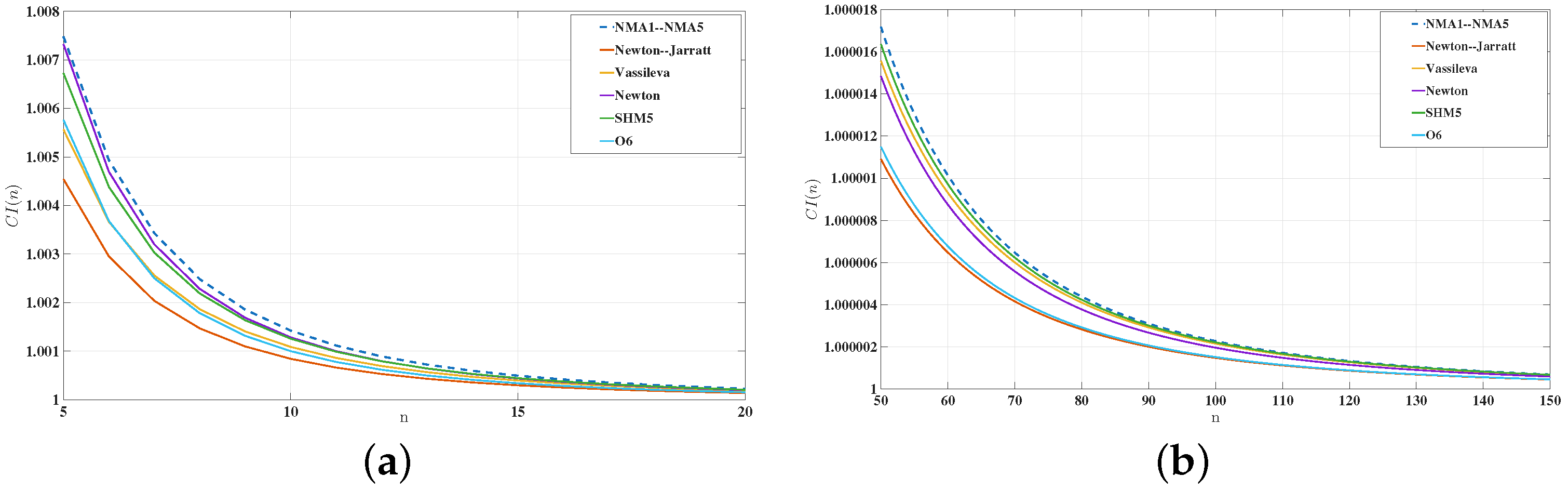
For a clearer visualization of the results in Table 3, Figure 1 displays the behavior of CI ( n ) for the proposed weighted family and the comparison methods in both small- and large-dimensional regimes.
The graphs confirm that, although the computational efficiency index decreases with the problem dimension for all schemes, the proposed weighted family maintains one of the most favorable behaviors in both the small- and large-dimensional regimes.

4.2. Relation with HPM, JFNK and Data-Driven PDE Solvers

The proposed method belongs to the class of deterministic high-order local solvers for finite-dimensional nonlinear systems. Therefore, its role is different from that of semi-analytical homotopy techniques, large-scale Newton–Krylov solvers, and data-driven PDE solvers. Table 4 summarizes these differences.

Solution of Some Academic Problems

This section presents a numerical assessment of the iterative schemes under a common computational framework. All experiments were performed on a computer running macOS Tahoe, version 26.4, equipped with an Apple M2 processor and 8 GB of RAM. For every method and test problem, the stopping criterion was
x ( k + 1 ) x ( k )   +   F ( x ( k + 1 ) )   < 10 100 ,
with a maximum of 50 iterations.
This criterion combines two complementary quantities: the increment between consecutive iterates and the nonlinear residual at the new approximation. Hence, the iteration is stopped only when both the correction step and the residual are sufficiently small. The tolerance 10 100 was chosen to study the asymptotic behavior of the high-order methods under controlled numerical conditions.
Variable precision arithmetic with 1500 significant digits was used to reduce the influence of round-off errors and to avoid premature numerical saturation. This is particularly relevant for fifth-order methods, since the error may decrease very rapidly and standard double precision may not allow the asymptotic convergence regime to be clearly observed. Therefore, the high-precision setting is used here as a verification framework for comparing local convergence behavior, not as a standard practical configuration for engineering computations. In practical double-precision implementations, the tolerance should be chosen according to machine precision, the conditioning of the nonlinear system, and the desired accuracy.
Each iterative scheme was executed 10 times for every test problem, and the reported execution time corresponds to the average value. The tables report the number of iterations, the final increment norm
x ( k + 1 ) x ( k ) ,
the final residual norm
F ( x ( k + 1 ) ) ,
the average execution time, and the approximated computational order of convergence (ACOC), see [12]. Whenever an exact solution is available, we also report the final discrete error and, when appropriate, the classical computational order of convergence (COC), see [13].
Example 1.
We begin with the nonlinear system of n equations
x i 1.5 sin j = 1 j i n x j = 0 , i = 1 , 2 , , n ,
with n = 40 , whose solution is
ξ 0.2375825578 , , 0.2375825578 T .
The initial approximation was taken as
x ( 0 ) = 1 4 , , 1 4 T .
Example 2.
We next consider the nonlinear system
x i cos j = 1 n x j + 2 x i = 0 , i = 1 , 2 , , n ,
with n = 30 , whose solution is
ξ 0.4867431909 , , 0.4867431909 T .
As initial guess, we used
x ( 0 ) = 1 2 , , 1 2 T .
Example 3.
Consider now the nonlinear system
x i + 5 2 log 1 + j = 1 j i n x j = 0 , i = 1 , 2 , , n ,
with n = 25 , whose solution is
ξ 4.2863062097 , , 4.2863062097 T .
The seed was chosen as
x ( 0 ) = 4 , , 4 T .
Example 4.
We now analyze the nonlinear system
x 1 + log ( 2 + x 1 + x 2 ) = 0 , x 2 + log ( 2 + x 2 + x 3 ) = 0 , x 998 + log ( 2 + x 998 + x 999 ) = 0 , x 999 + log ( 2 + x 999 + x 1 ) = 0 ,
where n = 999 . Its solution is approximately
ξ ( 0.3149230578 , , 0.3149230578 ) T .
The initial approximation was taken as
x ( 0 ) = 1 10 , , 1 10 T .
Example 5.
We now consider the nonlinear system
x 1 sin ( x 2 ) 1 = 0 , x 2 sin ( x 3 ) 1 = 0 , x 499 sin ( x 500 ) 1 = 0 , x 500 sin ( x 1 ) 1 = 0 ,
with n = 500 . The corresponding solution is
ξ ( 1.1141571409 , , 1.1141571409 ) T .
The initial approximation was taken as
x ( 0 ) = 1 2 , , 1 2 T .
Example 6.
We also study the nonlinear system
x 1 x 2 1 = 0 , x 2 x 3 1 = 0 , x 1498 x 1499 1 = 0 , x 1499 x 1 1 = 0 ,
with n = 1499 . In this case, the solution is
ξ 1.0000000000 , , 1.0000000000 T .
The initial approximation was chosen as
x ( 0 ) = 3 2 , , 3 2 T .
Example 7.
Finally, we consider the nonlinear system
x 1 x 2 e x 1 e x 2 = 0 , x 2 x 3 e x 2 e x 3 = 0 , x 1498 x 1499 e x 1498 e x 1499 = 0 , x 1499 x 1 e x 1499 e x 1 = 0 ,
with n = 1499 . Its solution is approximately
ξ ( 0.9012010317 , , 0.9012010317 ) T .
The initial estimate was taken as
x ( 0 ) = 6 5 , , 6 5 T .
In the seven test problems listed in Table 5, Table 6, Table 7, Table 8, Table 9, Table 10 and Table 11, the proposed family NMA1, …, NMA5 demonstrates consistently competitive performance. In all cases, the NMA variants converge in only three or four iterations, whereas Newton requires seven or eight iterations. Moreover, among the high-order methods, at least one NMA variant attains the lowest execution time in every example. When Newton is also included in the comparison, an NMA variant remains the fastest method in six of the seven tests. The only exception is Example (5), where Newton gives the lowest runtime; even in this case, the NMA variants are clearly faster than Newton–Jarratt, Vassileva, SHM5, and SH5. In addition, the observed values of p remain close to the theoretical order five in most cases, confirming that the proposed weighted family provides a robust and efficient alternative for solving large-scale nonlinear systems.

5. Application to a Stationary Viscous Burgers Problem

In order to illustrate the applicability of the proposed iterative family to nonlinear differential models, we consider a stationary one-dimensional viscous Burgers problem. This equation is a classical nonlinear model describing the interaction between convection and diffusion, and it is frequently used as a prototype in fluid mechanics, transport phenomena, and nonlinear wave propagation [20].
We study the boundary value problem
ρ u ( x ) + u ( x ) u ( x ) = f ( x ) , x ( 0 , 1 ) ,
subject to the homogeneous Dirichlet boundary conditions
u ( 0 ) = 0 , u ( 1 ) = 0 ,
where ρ > 0 denotes the viscosity parameter.
In order to validate the numerical solution, we use the method of manufactured solutions [21,22]. More precisely, we prescribe the exact solution
u ( x ) = x ( 1 x ) ,
which satisfies the boundary conditions (15). Its derivatives are
u ( x ) = 1 2 x , u ( x ) = 2 .
Substituting (16) into (14), the forcing term is obtained as
f ( x ) = ρ u ( x ) + u ( x ) u ( x ) = 2 ρ + x ( 1 x ) ( 1 2 x ) .
Therefore, the model problem under consideration is
ρ u ( x ) + u ( x ) u ( x ) = 2 ρ + x ( 1 x ) ( 1 2 x ) , x ( 0 , 1 ) ,
with
u ( 0 ) = 0 , u ( 1 ) = 0 .
The choice of this model is convenient for two reasons. First, it preserves the nonlinear convection–diffusion structure characteristic of Burgers-type equations [20]. Second, the exact solution is explicitly known, which allows us to verify the quality of the discrete approximation and to assess the performance of the iterative methods on the nonlinear algebraic system arising from the discretization.
  • Finite-difference discretization
Let N be the number of interior nodes and define the uniform mesh
x i = i h , i = 0 , 1 , , N + 1 ,
with mesh size
h = 1 N + 1 .
At the interior nodes x i , i = 1 , , N , we denote by
u i u ( x i )
the numerical approximation of the exact solution.
To discretize the derivatives, we employ the standard centered finite-difference formulas [23]. For the second derivative, we use
u ( x i ) u i 1 2 u i + u i + 1 h 2 ,
while for the first derivative we take
u ( x i ) u i + 1 u i 1 2 h .
Substituting (19) and (20) into (18), we obtain, for each interior node x i ,
ρ u i 1 2 u i + u i + 1 h 2 + u i u i + 1 u i 1 2 h f ( x i ) = 0 , i = 1 , , N .
Using the boundary conditions,
u 0 = 0 , u N + 1 = 0 ,
the discrete problem becomes a nonlinear system of N equations with N unknowns.
  • Nonlinear algebraic system
Let U = ( u 1 , u 2 , , u N ) T R N . The nonlinear system can be written in compact form as
F ( U ) = 0 ,
where F ( U ) = ( F 1 ( U ) , F 2 ( U ) , , F N ( U ) ) T , with components given by
F i ( U ) = ρ u i 1 2 u i + u i + 1 h 2 + u i u i + 1 u i 1 2 h f ( x i ) , i = 1 , , N ,
together with the conventions
u 0 = 0 , u N + 1 = 0 .
More explicitly, the first and last equations read
F 1 ( U ) = ρ 2 u 1 + u 2 h 2 + u 1 u 2 2 h f ( x 1 ) ,
F N ( U ) = ρ u N 1 2 u N h 2 u N u N 1 2 h f ( x N ) ,
while for i = 2 , , N 1 ,
F i ( U ) = ρ u i 1 2 u i + u i + 1 h 2 + u i u i + 1 u i 1 2 h f ( x i ) .
This system is nonlinear because of the convective term
u i u i + 1 u i 1 2 h .
Consequently, an iterative method is required in order to compute the discrete solution.
  • Jacobian matrix
Since the methods considered in this work require the Jacobian matrix, we now derive its explicit form. Differentiating (22) with respect to the neighboring unknowns, we obtain
F i u i 1 = ρ h 2 u i 2 h ,
F i u i = 2 ρ h 2 + u i + 1 u i 1 2 h ,
F i u i + 1 = ρ h 2 + u i 2 h .
All other partial derivatives are zero. Therefore, the Jacobian matrix
J ( U ) = F ( U )
is tridiagonal and can be written as
J ( U ) = 2 ρ h 2 + u 2 2 h ρ h 2 + u 1 2 h 0 0 ρ h 2 u 2 2 h 2 ρ h 2 + u 3 u 1 2 h ρ h 2 + u 2 2 h 0 ρ h 2 u 3 2 h 2 ρ h 2 + u 4 u 2 2 h 0 ρ h 2 + u N 1 2 h 0 0 ρ h 2 u N 2 h 2 ρ h 2 u N 1 2 h .
Hence, the discrete problem (21) leads to a sparse nonlinear algebraic system whose Jacobian has a structured tridiagonal form. This makes it especially suitable for assessing the practical performance of the iterative methods studied in this work.
  • Numerical solution procedure
To solve the nonlinear system (21), one may choose as initial approximation, for instance,
U ( 0 ) = ( 0 , 0 , , 0 ) T ,
or, if desired, the exact solution sampled at the grid points plus a small perturbation. Once the mesh size h, the viscosity parameter ρ , and the forcing term f ( x i ) are fixed, the iterative schemes are applied directly to the nonlinear system (21).
For each computed approximation U ( k ) , the quality of the numerical solution may be assessed through the residual norm
F ( U ( k ) ) ,
and, since the exact solution is known, also through the discrete error
E ( k ) = max 1 i N | u i u ( x i ) | .
This allows us to compare not only the convergence speed of the iterative methods, but also the accuracy of the final discrete approximation. The previous construction provides a complete test framework: a nonlinear differential model of physical interest, a manufactured exact solution, a finite-difference discretization, and an explicit nonlinear algebraic system. Therefore, the stationary Burgers problem constitutes a suitable benchmark for validating the theoretical and practical performance of the proposed high-order iterative family [20].
For the numerical solution of the nonlinear algebraic system arising from the finite-difference discretization of the stationary Burgers problem, we considered N = 300 interior nodes, viscosity parameter ρ = 0.09 , and mesh size h = 0.00332226 . The stopping criterion was fixed as
x ( k + 1 ) x ( k )   +   F ( x ( k + 1 ) )   < 10 100 ,
with a maximum of 50 iterations. Table 12 reports, for each method, the total number of iterations, the increment norm x ( k + 1 ) x ( k ) , the residual norm F ( x ( k + 1 ) ) , the execution time in seconds, the approximated computational order of convergence (ACOC), and, when the exact solution is used, the computational order of convergence (COC), together with the infinity norm of the error.

5.1. On the Observed ACOC and COC in the Burgers Experiment

Although the proposed family has theoretical local order five, the computational orders obtained for the Burgers problem are close to four for the NMA variants. This does not contradict the convergence theorem, since the theoretical result is asymptotic, whereas the numerical test involves a finite-difference discretization, a finite mesh, and a nonlinear system whose Jacobian depends on the mesh size h and the viscosity parameter ρ .
In Table 12, the NMA methods converge in only four iterations. Thus, only a few consecutive error ratios are available to estimate the order. Moreover, the stringent stopping criterion
x ( k + 1 ) x ( k )   +   F ( x ( k + 1 ) )   < 10 100
may stop the process before a sufficiently long fifth-order asymptotic regime is numerically visible. Mesh effects, conditioning of the discrete Jacobian, and numerical saturation at very small residual levels can also influence the observed order.
Since the Burgers problem has a manufactured exact solution, we also computed the classical computational order of convergence (COC), based on the true errors. The ACOC and COC values reported in Table 12 are very similar for NMA1–NMA5, which indicates that the observed reduction is not merely an artifact of the ACOC estimator. Rather, it reflects the numerical behavior of this particular discretized problem under the selected mesh, viscosity, initial approximation, and stopping criterion. Therefore, these computational orders should be interpreted as numerical indicators and do not invalidate the fifth-order local convergence established theoretically.

5.2. Graphical Analysis for the Stationary Burgers Problem

To complement the numerical results reported above, this subsection presents a graphical analysis of the performance of NMA2 when applied to the stationary Burgers problem. The visual comparison includes the agreement between the exact and numerical solutions, the distribution of the absolute error, the convergence history of the selected methods, and the evolution of the iterates generated during the nonlinear resolution process.
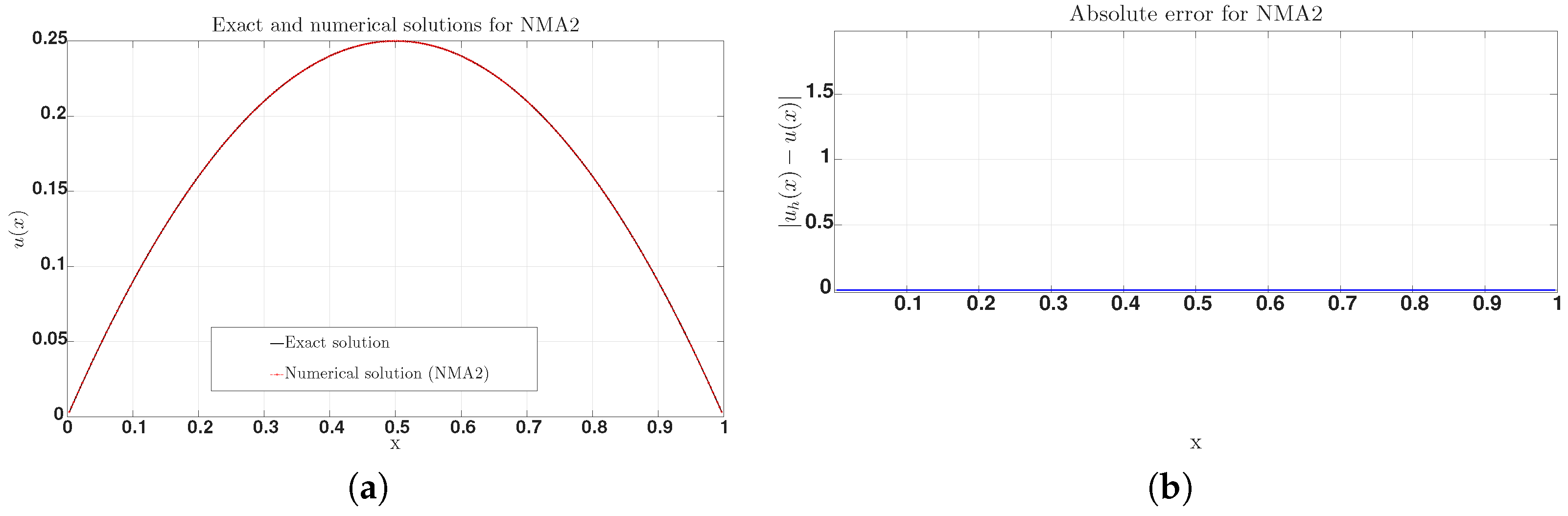
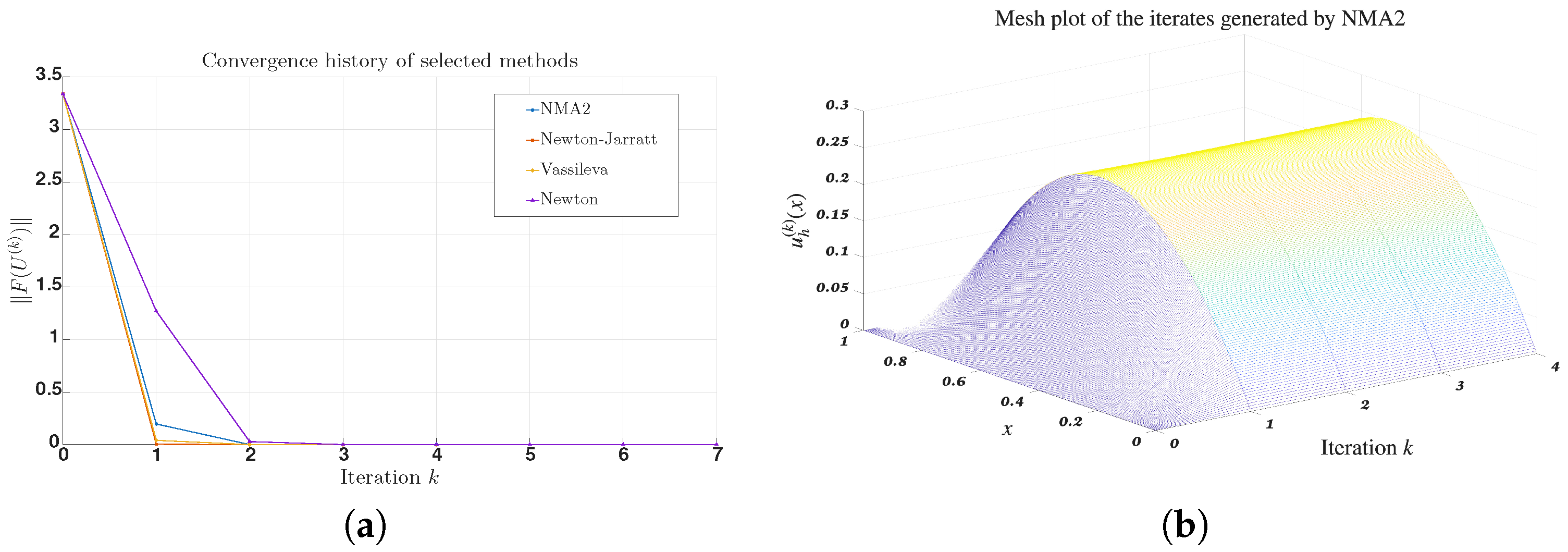
Figure 2a,b show that the numerical solution obtained with NMA2 is practically indistinguishable from the exact solution and that the absolute error remains negligible over the computational mesh. Figure 3a confirms the fast decrease in the residual norm for NMA2 compared with the reference methods, while Figure 3b illustrates the stable evolution of the iterates toward the final discrete solution. Overall, these plots provide graphical evidence of the accuracy, stability, and fast convergence of NMA2 for this nonlinear differential problem.

Robustness with Respect to the Initial Approximation

Since the convergence result established in Section 3 is local, we added robustness tests with different initial approximations. The purpose of these experiments is not to prove global convergence, but to provide numerical evidence about the stability of the proposed weighted family when the starting point is perturbed.
For the algebraic systems, we considered initial approximations of the form
x η ( 0 ) = ξ + η v ,
where v is a fixed normalized perturbation vector and η controls the distance from the root. For the Burgers problem, we considered the zero vector, constant initial profiles, and perturbations of the manufactured solution.
All tests were performed using the same stopping criterion and maximum number of iterations as in the previous experiments.
The robustness results in Table 13 show that the proposed schemes preserve convergence under moderate perturbations of the initial approximation. For Example 1, both NMA1 and NMA2 converge for all tested values of η , requiring only three or four iterations and reaching very small final residuals.
For the stationary Burgers equation, NMA2 also converges from the three initial profiles considered. In this case, the ACOC values 3.97681 , 3.97219 , and 4.00792 remain close to four, confirming a stable high-order behavior even in the discretized nonlinear PDE setting. These results support the numerical robustness of the proposed family, although the theoretical convergence result remains local.

5.3. Limitations and Practical Applicability

The convergence analysis developed in this work is local. Therefore, the initial approximation must be sufficiently close to a simple root of the nonlinear system. The present paper does not establish semilocal or global convergence. A semilocal theory would require additional assumptions, such as explicit bounds on F ( x ) 1 , Lipschitz-type conditions on F , and a majorizing sequence argument. These topics are beyond the scope of the present contribution.
The proposed methods also require the solution of two linear systems per iteration involving Jacobian matrices evaluated at x ( k ) and y ( k ) . Consequently, the methods are most appropriate when the Jacobian matrix is available analytically, can be computed accurately, or has an exploitable sparse or structured form. In the Burgers discretization considered here, the Jacobian matrix is tridiagonal, which makes the problem more favorable than a fully dense nonlinear system.
The assumption that F ( ξ ) is nonsingular implies, by continuity of F , that F ( x ) remains nonsingular in a sufficiently small neighborhood of ξ . The local convergence analysis is restricted to iterates lying in such a neighborhood. If the Jacobian becomes nearly singular, the constants appearing in the local error equation may become large, the linear solves may be ill-conditioned, and the expected high-order behavior may deteriorate.
In near-singular or poorly conditioned cases, damping strategies, trust-region safeguards, pivoting techniques, regularization, or preconditioned Jacobian-free variants may be required. Thus, the proposed family should be viewed as a high-order deterministic local solver for smooth nonlinear systems, rather than as a globally convergent black-box method for arbitrary nonsmooth, ill-conditioned, or very large-scale problems.

6. Conclusions

We introduced a weighted family of fifth-order iterative methods for solving smooth systems of nonlinear equations. The proposed schemes include Singh–Sharma fifth-order method as a particular case and preserve the same local convergence order under suitable conditions on the weight functions. The leading error equation shows that the weight function G can modify the principal error operator, providing additional flexibility without changing the basic evaluation structure.
The numerical experiments show that the proposed variants are competitive with several fifth-order reference methods in terms of residual decay, number of iterations, execution time, ACOC, and computational efficiency index. The application to the stationary viscous Burgers problem illustrates the behavior of the family on a nonlinear algebraic system arising from a finite-difference discretization with structured Jacobian.
The method is local and requires nonsingular Jacobians in a neighborhood of the solution. Therefore, its most natural use is in smooth problems where the Jacobian is available or structured. Future work will address semilocal convergence, globalization strategies, Jacobian-free variants, and applications to more demanding nonlinear PDE discretizations.


Author Contributions

Conceptualization, N.U.C.; methodology, N.U.C., M.A.L.S. and A.R.C.; software, N.U.C., M.A.L.S. and A.R.C.; validation, N.U.C. and A.R.C.; formal analysis, N.U.C., M.A.L.S.; investigation, N.U.C., M.A.L.S. and A.R.C.; visualization, A.R.C.; supervision, J.G.M.; writing—original draft preparation, N.U.C.; writing—review and editing, J.G.M., N.U.C., M.A.L.S. and A.R.C. All authors have read and agreed to the published version of the manuscript.

Funding

This research was funded by the Fondo Nacional de Innovación y Desarrollo Científico y Tecnológico (FONDOCYT) of the Ministerio de Educación Superior, Ciencia y Tecnología de la República Dominicana (MESCyT), under grant number FONDOCYT 2023-1-1D2-0537.

Data Availability Statement

The original contributions presented in this study are included in the article. Further inquiries can be directed to the corresponding author.

Acknowledgments

The authors gratefully acknowledge the institutional support provided by ISFODOSU, UNAPEC, UASD, and INTEC, which made this research possible. The authors also express their special appreciation to the Instituto Tecnológico de Santo Domingo (INTEC), where N.U.C. is currently pursuing doctoral studies, as this article forms part of that doctoral research. The authors sincerely thank the reviewers for their careful evaluation of our manuscript and for their valuable comments and suggestions. We believe that their observations were very insightful and have helped us to substantially improve the quality, clarity, and presentation of the paper.

Conflicts of Interest

The authors declare no conflicts of interest.

Notation

Main notation used throughout the manuscript.
SymbolMeaning
F : Ω R n R n Nonlinear operator.
ξ Simple root of the nonlinear system F ( x ) = 0 .
F ( x ) Jacobian matrix of F at x.
e ( k ) = x ( k ) ξ Local error at iteration k.
C q = 1 q ! [ F ( ξ ) ] 1 F ( q ) ( ξ ) Normalized higher-order derivative operator.
H, GScalar weight functions used in the correction step.
ν k Residual ratio used in the weighted correction.
pTheoretical order of convergence.
ACOCApproximated computational order of convergence.
COCComputational order of convergence.
C I ( n ) Computational efficiency index for systems of dimension n.
NNumber of interior grid points in the finite-difference discretization.
hMesh size.
ρ Viscosity parameter in the stationary Burgers equation.

References

  1. Ortega, J.M.; Rheinboldt, W.C. Iterative Solution of Nonlinear Equations in Several Variables; Academic Press: Cambridge, MA, USA, 1970. [Google Scholar]
  2. Kelley, C.T. Solving Nonlinear Equations with Newton’s Method; SIAM: Philadelphia, PA, USA, 2003. [Google Scholar] [CrossRef] [Scilit]
  3. Kung, H.T.; Traub, J.F. Optimal Order of One-Point and Multipoint Iteration. J. ACM 1974, 21, 643–651. [Google Scholar] [CrossRef] [Scilit]
  4. Jaiswal, J.P. A Class of Iterative Methods for Solving Nonlinear Equation with Fourth-Order Convergence. arXiv 2013, arXiv:1307.7334. [Google Scholar] [CrossRef] [Scilit]
  5. Artidiello, S.; Cordero, A.; Torregrosa, J.R.; Vassileva, M.P. Multidimensional Generalization of Iterative Methods for Solving Nonlinear Problems by Means of Weight-Function Procedure. Appl. Math. Comput. 2015, 268, 1064–1071. [Google Scholar] [CrossRef] [Scilit]
  6. Artidiello, S.; Cordero, A.; Torregrosa, J.R.; Vassileva, M.P. Design of High-Order Iterative Methods for Nonlinear Systems by Using Weight Function Procedure. Abstr. Appl. Anal. 2015, 2015, 289029. [Google Scholar] [CrossRef] [Scilit]
  7. Sharma, J.R.; Arora, H. On Efficient Weighted-Newton Methods for Solving Systems of Nonlinear Equations. Appl. Math. Comput. 2013, 222, 497–506. [Google Scholar] [CrossRef] [Scilit]
  8. Capdevila, R.R.; Cordero, A.; Torregrosa, J.R. A New Three-Step Class of Iterative Methods for Solving Nonlinear Systems. Mathematics 2019, 7, 1221. [Google Scholar] [CrossRef] [Scilit]
  9. Singh, H.; Sharma, J.R. Simple and Efficient Fifth Order Solvers for Systems of Nonlinear Problems. Math. Model. Anal. 2023, 28, 1–22. [Google Scholar] [CrossRef] [Scilit]
  10. Burns, J.; Balogh, A.; Gilliam, D.S.; Shubov, V.I. Numerical Stationary Solutions for a Viscous Burgers’ Equation. J. Math. Syst. Estim. Control 1998, 8, 253–256. [Google Scholar]
  11. Taigbenu, A.E.; Onyejekwe, O.O. A Mixed Green Element Formulation for the Transient Burgers Equation. Int. J. Numer. Methods Fluids 1997, 24, 563–578. [Google Scholar] [CrossRef]
  12. Cordero, A.; Torregrosa, J.R. Variants of Newton’s Method Using Fifth-Order Quadrature Formulas. Appl. Math. Comput. 2007, 190, 686–698. [Google Scholar] [CrossRef] [Scilit]
  13. Weerakoon, S.; Fernando, T.G.I. A Variant of Newton’s Method with Accelerated Third-Order Convergence. Appl. Math. Lett. 2000, 13, 87–93. [Google Scholar] [CrossRef] [Scilit]
  14. Cordero, A.; Hueso, J.L.; Martínez, E.; Torregrosa, J.R. A Modified Newton-Jarratt’s Composition. Numer. Algorithms 2010, 55, 87–99. [Google Scholar] [CrossRef] [Scilit]
  15. Arroyo, V.; Cordero, A.; Torregrosa, J.R.; Vassileva, M.P. Artificial Satellites Preliminary Orbit Determination by the Modified High-Order Gauss Method. Int. J. Comput. Math. 2012, 89, 347–356. [Google Scholar] [CrossRef] [Scilit]
  16. Sharma, J.R.; Gupta, P. An Efficient Fifth Order Method for Solving Systems of Nonlinear Equations. Comput. Math. Appl. 2014, 67, 591–601. [Google Scholar] [CrossRef] [Scilit]
  17. Solaiman, O.S.; Hashim, I. An Iterative Scheme of Arbitrary Odd Order and Its Basins of Attraction for Nonlinear Systems. Comput. Mater. Contin. 2021, 66, 1427–1444. [Google Scholar] [CrossRef] [Scilit]
  18. Arroyo, V.; Cordero, A.; Torregrosa, J.R. Approximation of Artificial Satellites’ Preliminary Orbits: The Efficiency Challenge. Math. Comput. Model. 2011, 54, 1802–1807. [Google Scholar] [CrossRef] [Scilit]
  19. Grau-Sánchez, M.; Grau, Á.; Noguera, M. On the Computational Efficiency Index and Some Iterative Methods for Solving Systems of Non-Linear Equations. J. Comput. Appl. Math. 2011, 236, 1259–1266. [Google Scholar] [CrossRef] [Scilit]
  20. Bonkile, M.P.; Awasthi, A.; Lakshmi, C.; Mukundan, V.; Aswin, V.S. A Systematic Literature Review of Burgers’ Equation with Recent Advances. Pramana 2018, 90, 69. [Google Scholar] [CrossRef] [Scilit]
  21. Oberkampf, W.L.; Roy, C.J. Exact Solutions. In Verification and Validation in Scientific Computing; Cambridge University Press: Cambridge, UK, 2010; pp. 208–248. [Google Scholar] [CrossRef] [Scilit]
  22. Roy, C.J. Review of Code and Solution Verification Procedures for Computational Simulation. J. Comput. Phys. 2005, 205, 131–156. [Google Scholar] [CrossRef] [Scilit]
  23. Morton, K.W.; Mayers, D.F. Numerical Solution of Partial Differential Equations: An Introduction, 2nd ed.; Cambridge University Press: Cambridge, UK, 2005. [Google Scholar]
Figure 1. Computational efficiency indices of the proposed weighted family NMA1–NMA5 and the reference methods. (a) Computational efficiency index in the small-dimensional regime. (b) Computational efficiency index in the large-dimensional regime.
Mathematics 14 01944 g001
Figure 2. Stationary Burgers problem with N = 300 , ρ = 0.09 , h = 0.00332226 , tolerance 10 100 , and initial guess U ( 0 ) = 0 . (a) Exact and numerical solutions obtained with NMA2. (b) Absolute pointwise error in logarithmic scale.
Mathematics 14 01944 g002
Figure 3. Convergence behavior for the stationary Burgers problem with N = 300 , ρ = 0.09 , h = 0.00332226 , tolerance 10 100 , and initial guess U ( 0 ) = 0 . (a) Residual decay for selected methods. (b) Evolution of the iterates generated by NMA2.
Mathematics 14 01944 g003
Table 1. Correspondence between the labels NMA1–NMA5 and the selected weight functions used in the numerical experiments.
MethodSource in Proposition 1 H ( ν ) G ( ν )
NMA1Case (i) 1 + ν 0
NMA2Case (ii) 1 + ν + α ν 2 , α = 1 2 0
NMA3Case (iii) 1 + ν γ ν 2 , γ = 1
NMA4Case (iv) 1 + ν + α ν 2 , α = 1 2 β ν 2 , β = 1 4
NMA5Case (v) 1 + ν + a ν 3 , a = 1 2 0
Table 2. Per-iteration counts for the proposed weighted family and the comparison methods.
MethodOrder p n F n J n LU n V ( n MV , n A )
NMA1–NMA552222 ( 0 , 0 )
Newton–Jarratt52233 ( 1 , 3 )
Vassileva52223 ( 1 , 2 )
Newton21111 ( 0 , 0 )
SHM552224 ( 0 , 0 )
SH552233 ( 0 , 1 )
Table 3. Computational efficiency indices for the proposed weighted family and the comparison methods.
MethodOrder p d ( n ) op ( n ) CI ( n )
NMA1–NMA55 2 n + 2 n 2 2 3 n 3 + 2 n 2 + 10 3 n + 1 5 1 2 3 n 3 + 4 n 2 + 16 3 n + 1
Newton–Jarratt5 2 n + 2 n 2 n 3 + 7 n 2 n 5 1 n 3 + 9 n 2 + n
Vassileva5 2 n + 2 n 2 2 3 n 3 + 6 n 2 2 3 n 5 1 2 3 n 3 + 8 n 2 + 4 3 n
Newton2 n + n 2 n 3 3 + n 2 n 3 2 1 n 3 3 + 2 n 2 + 2 3 n
SHM55 2 n + 2 n 2 2 3 n 3 + 4 n 2 2 3 n 5 1 2 3 n 3 + 6 n 2 + 4 3 n
SH55 2 n + 2 n 2 n 3 + 4 n 2 n 5 1 n 3 + 6 n 2 + n
Note. The cost model assumes dense LU factorization. If the Jacobian matrix is sparse, banded, or tridiagonal, as in the Burgers discretization considered in this work, the algebraic cost may be reduced by using structure-preserving linear solvers. Scalar evaluations of the weight functions are negligible compared with Jacobian factorizations and linear solves.
Table 4. Positioning of the proposed weighted family with respect to other modern approaches.
ApproachMain PurposeMain AdvantageRelation with the Present Work
HPMSemi-analytical approximation of nonlinear differential models.Can provide analytical or series-type approximations.Complementary approach; it is not primarily designed as a general algebraic solver for F ( x ) = 0 .
JFNKLarge-scale nonlinear systems, usually sparse.Avoids explicit Jacobian storage by using Jacobian-vector products.Natural competitor for very large-scale problems; usually requires Krylov solvers and preconditioning.
PINNs/DeepONet/FNOData-driven solution or learning of PDE solution operators.Useful for parametric problems, inverse problems, or repeated-query regimes.Complementary approach; requires training data, architecture selection, and optimization.
Proposed familySmooth nonlinear systems with available or structured Jacobian.Fifth-order local convergence, explicit error equation, no training stage.Useful when high local accuracy is required and Jacobian information is available or exploitable.
Table 5. Numerical results Example 1.
MethodIter x ( k + 1 ) x ( k ) F ( x ( k + 1 ) ) E-Time (s)p
NMA13 4.40536 × 10 25 3.08917 × 10 120 4.5717655.01373
NMA23 4.41439 × 10 25 3.12094 × 10 120 3.8670255.01378
NMA33 4.15111 × 10 25 2.27463 × 10 120 4.0652865.01357
NMA43 4.28547 × 10 25 2.67921 × 10 120 3.8339855.01370
NMA53 4.40537 × 10 25 3.08920 × 10 120 4.0797265.01373
Newton-Jarratt3 2.25458 × 10 29 6.59569 × 10 142 6.0687674.88328
Vassileva3 1.78313 × 10 26 1.64851 × 10 127 4.5392565.03546
Newton7 1.01862 × 10 89 2.96422 × 10 177 3.9853712.00000
SHM54 7.37388 × 10 101 2.36458 × 10 498 8.2096924.99999
SH54 7.12497 × 10 102 1.90005 × 10 503 7.4280334.99999
Table 6. Numerical results Example 2.
MethodIter x ( k + 1 ) x ( k ) F ( x ( k + 1 ) ) E-Time (s)p
NMA13 1.56308 × 10 24 7.05278 × 10 117 1.2296984.78733
NMA23 1.55782 × 10 24 6.93474 × 10 117 1.2200304.78727
NMA33 1.35989 × 10 24 3.30788 × 10 117 1.2976594.79270
NMA43 1.45390 × 10 24 4.76549 × 10 117 1.7694454.78991
NMA53 1.56308 × 10 24 7.05267 × 10 117 1.9344134.78733
Newton-Jarratt3 2.61841 × 10 25 4.54841 × 10 121 3.1294744.84655
Vassileva3 1.78162 × 10 26 5.98323 × 10 127 2.0178814.81223
Newton7 8.13592 × 10 76 2.30589 × 10 149 1.9085112.00000
SHM53 4.16381 × 10 22 1.28006 × 10 104 3.3959964.85400
SH53 2.10691 × 10 22 3.09126 × 10 106 2.5824384.88575
Table 7. Numerical results Example 3.
MethodIter x ( k + 1 ) x ( k ) F ( x ( k + 1 ) ) E-Time (s)p
NMA13 1.72503 × 10 31 9.06254 × 10 161 1.7738925.04246
NMA23 1.75072 × 10 31 9.75767 × 10 161 1.0566555.04273
NMA33 1.01957 × 10 31 6.07636 × 10 162 1.3388785.04066
NMA43 1.35466 × 10 31 2.61131 × 10 161 1.0046155.04186
NMA53 1.72505 × 10 31 9.06293 × 10 161 1.3683455.04246
Newton-Jarratt3 2.22399 × 10 33 1.72852 × 10 170 1.5470625.03030
Vassileva3 7.30792 × 10 34 5.31269 × 10 173 1.4231585.03316
Newton7 6.83086 × 10 96 4.98209 × 10 193 1.2792602.00000
SHM53 4.67693 × 10 31 1.64143 × 10 158 1.8729045.03829
SH53 3.47083 × 10 32 2.52697 × 10 164 1.6655045.03156
Table 8. Numerical results Example 4.
MethodIter x ( k + 1 ) x ( k ) F ( x ( k + 1 ) ) E-Time (s)p
NMA13 5.59822 × 10 20 2.35377 × 10 104 46.3055674.96232
NMA23 4.00910 × 10 20 4.43353 × 10 105 31.5546484.95423
NMA34 7.15683 × 10 99 1.61802 × 10 498 47.1044335.00001
NMA43 1.78288 × 10 19 1.16174 × 10 101 49.8491654.92781
NMA53 5.57978 × 10 20 2.31525 × 10 104 32.1385654.96224
Newton-Jarratt3 6.71738 × 10 21 9.73981 × 10 109 82.9237794.84142
Vassileva3 2.04247 × 10 20 2.30225 × 10 106 72.7154964.87793
Newton7 1.31659 × 10 51 5.84264 × 10 104 37.2493522.00000
SHM53 3.27215 × 10 26 8.98197 × 10 136 53.5383414.76765
SH53 4.01239 × 10 22 5.41699 × 10 115 55.6995224.82924
Table 9. Numerical results Example 5.
MethodIter x ( k + 1 ) x ( k ) F ( x ( k + 1 ) ) E-Time (s)p
NMA14 4.75186 × 10 57 1.87800 × 10 290 5.0535104.86902
NMA24 2.61307 × 10 57 9.44344 × 10 292 5.0698334.85266
NMA34 4.32898 × 10 57 1.17704 × 10 290 5.5437404.90295
NMA44 5.26546 × 10 57 3.13548 × 10 290 5.1789514.87371
NMA54 4.61617 × 10 57 1.62474 × 10 290 5.0300634.86792
Newton-Jarratt4 7.48230 × 10 72 1.39428 × 10 364 12.0465904.99301
Vassileva4 1.25643 × 10 64 1.21067 × 10 328 10.1436974.96929
Newton7 1.71434 × 10 52 7.76332 × 10 107 4.4508202.00000
SHM54 8.46222 × 10 48 1.36169 × 10 242 7.4261864.99853
SH54 1.12576 × 10 55 5.63851 × 10 282 8.0661044.99946
Table 10. Numerical results Example 6.
MethodIter x ( k + 1 ) x ( k ) F ( x ( k + 1 ) ) E-Time (s)p
NMA14 2.89142 × 10 72 4.49701 × 10 365 40.1819664.99977
NMA24 2.30690 × 10 72 1.45382 × 10 365 37.0762014.99977
NMA34 2.44813 × 10 73 1.71219 × 10 370 37.2031644.99980
NMA44 6.84615 × 10 73 3.13741 × 10 368 37.4452494.99978
NMA54 2.88517 × 10 72 4.44862 × 10 365 37.3312724.99977
Newton-Jarratt4 1.99479 × 10 82 2.34278 × 10 416 120.8741954.99993
Vassileva4 3.06274 × 10 82 2.24879 × 10 415 91.7317544.99992
Newton8 2.63494 × 10 88 1.79325 × 10 177 41.0928532.00000
SHM54 2.00539 × 10 71 7.21710 × 10 361 60.3794904.99977
SH54 2.50728 × 10 78 1.10243 × 10 395 71.9822224.99989
Table 11. Numerical results Example 7.
MethodIter x ( k + 1 ) x ( k ) F ( x ( k + 1 ) ) E-Time (s)p
NMA13 7.71284 × 10 26 1.68563 × 10 134 51.6787875.00302
NMA23 7.28725 × 10 26 1.26914 × 10 134 35.9187515.00189
NMA33 2.12069 × 10 26 1.98452 × 10 137 33.9131205.01158
NMA43 3.93658 × 10 26 5.10609 × 10 136 35.6291895.00558
NMA53 7.71200 × 10 26 1.68471 × 10 134 35.9473535.00302
Newton-Jarratt3 4.62153 × 10 32 1.09740 × 10 166 93.6376745.01071
Vassileva3 3.53465 × 10 29 8.49020 × 10 152 81.8963775.01417
Newton7 1.37639 × 10 73 2.90608 × 10 148 46.1802222.00000
SHM53 7.71927 × 10 26 1.58724 × 10 134 56.7985265.01074
SH53 3.84653 × 10 29 9.67519 × 10 152 66.5771145.04700
Table 12. Numerical results for the stationary Burgers problem.
MethodIter x ( k + 1 ) x ( k ) F ( x ( k + 1 ) ) E-Time (s) ACOC COC e
NMA14 6.64232 × 10 43 2.87746 × 10 172 19.6730854.088174.00333 2.335869 × 10 174
NMA24 1.96179 × 10 42 1.98705 × 10 170 20.1546824.090494.00403 1.512433 × 10 172
NMA34 1.02754 × 10 36 4.81522 × 10 147 19.6523084.005624.00854 6.057773 × 10 149
NMA44 6.40580 × 10 39 6.10708 × 10 156 19.7074013.971974.00815 5.656045 × 10 158
NMA54 7.20069 × 10 43 3.94650 × 10 172 19.6534824.088354.00338 3.191103 × 10 174
Newton-Jarratt3 9.61428 × 10 25 1.37166 × 10 124 24.6822524.963514.96385 1.127150 × 10 126
Vassileva4 3.69445 × 10 53 2.41590 × 10 214 22.4715844.049824.00636 3.324868 × 10 216
Newton7 6.28204 × 10 70 1.09130 × 10 139 17.1582942.000091.99743 1.139233 × 10 141
SHM54 1.49755 × 10 80 6.90493 × 10 404 29.7021395.020155.06151 0.000000 × 10 0
SH54 4.82856 × 10 95 3.66973 × 10 477 30.3694085.041285.06174 0.000000 × 10 0
Table 13. Robustness tests with respect to different initial approximations.
ProblemInitial ApproximationMethodConvergedIter x ( k + 1 ) x ( k ) F ( x ( k + 1 ) ) E-Time (s)ACOC
Example 1 ξ + 10 2 v NMA1Yes3 3.09457 × 10 22 5.28367 × 10 106 1.6984755.34098
Example 1 ξ + 10 1 v NMA1Yes4 1.35646 × 10 47 4.17463 × 10 233 2.4028924.75110
Example 1 ξ + 0.5 v NMA1Yes4 8.97222 × 10 51 1.08251 × 10 248 2.1976844.97174
Example 1 ξ + 10 2 v NMA2Yes3 3.19235 × 10 22 6.17286 × 10 106 2.4582485.34211
Example 1 ξ + 10 1 v NMA2Yes4 4.88540 × 10 44 2.52975 × 10 215 3.6287784.80254
Example 1 ξ + 0.5 v NMA2Yes4 1.90546 × 10 50 4.67667 × 10 247 5.0442744.97046
Burgers U ( 0 ) = 0 NMA2Yes4 1.74416 × 10 59 3.82181 × 10 238 12.8691083.97681
Burgers U ( 0 ) = 0.5  1NMA2Yes4 3.95164 × 10 42 1.05653 × 10 168 20.0417803.97219
Burgers U ( 0 ) = U + 0.1 sin ( π x i ) NMA2Yes4 3.20016 × 10 69 4.54389 × 10 277 16.6644174.00792
Disclaimer/Publisher’s Note: The statements, opinions and data contained in all publications are solely those of the individual author(s) and contributor(s) and not of MDPI and/or the editor(s). MDPI and/or the editor(s) disclaim responsibility for any injury to people or property resulting from any ideas, methods, instructions or products referred to in the content.