Article

Statistical Learning of Conditional Single-Index U-Processes Under Local Stationarity and Missing-At-Random Functional Responses


Université de Technologie de Compiègne, Alliance Sorbonne Université, LMAC, 60203 Compiègne, France
Mathematics 2026, 14(12), 2112; https://doi.org/10.3390/math14122112
Submission received: 22 April 2026 / Revised: 9 June 2026 / Accepted: 9 June 2026 / Published: 13 June 2026
(This article belongs to the Section D1: Probability and Statistics)

Abstract

This paper develops a unified asymptotic theory for conditional single-index U-statistics and the associated conditional U-processes in the setting of locally stationary functional time series subject to missing-at-random response mechanisms. The proposed framework addresses, within a single nonparametric inferential architecture, three major sources of complexity in modern functional data analysis: infinite-dimensional covariates, smoothly time-varying stochastic dynamics, and incomplete response observations. The methodology is based on a class of kernel-type estimators combining temporal localization, functional single-index smoothing, and inverse-propensity correction. Temporal localization captures the gradual evolution of the underlying regression structure, the single-index projection provides an effective dimension-reduction mechanism for functional covariates, and the propensity adjustment restores the target conditional functional under the MAR sampling scheme. The principal contribution of the paper is the establishment of weak convergence, in a suitable space of bounded functions, for the resulting propensity-adjusted conditional U-process indexed by a general class of measurable kernels. Under absolute regularity conditions, local stationarity assumptions, small-ball probability requirements, entropy restrictions of VC type, and uniform consistency of the propensity-score estimator, the normalized process is shown to converge weakly to a tight centered Gaussian process. The limiting covariance structure explicitly reflects the interaction between temporal smoothing, functional concentration, dependence, and the random loss of responses. In parallel, uniform convergence rates are derived for the associated conditional single-index U-statistic estimators, thereby quantifying the respective contributions of smoothing bias, stochastic fluctuation, local-stationarity approximation error, and missingness-induced variance inflation. A substantial part of the analysis is devoted to the technical difficulties created by the simultaneous presence of dependence, nonstationarity, functional covariates, and incomplete observations. The proofs combine Hoeffding-type decompositions adapted to weighted incomplete data, blocking and coupling arguments for absolutely regular triangular arrays, refined entropy bounds for kernel-indexed function classes, and small-ball probability techniques for functional covariates. The MAR mechanism is incorporated via inverse-propensity weighting, and its effects on the effective sample size, asymptotic variance, and bias structure are made explicit. The theory also provides a rigorous foundation for bandwidth selection through blocked, propensity-adjusted cross-validation and clarifies its relation to the corresponding oracle risk. The proposed framework encompasses a broad class of statistical learning and inference problems involving pairwise or higher-order functionals of functional time series. In particular, it applies to conditional Kendall-type functionals, discrimination problems, metric learning with incomplete labels, and conditional independence testing under local stationarity. A simulation study illustrates the finite-sample behavior of the proposed estimators and supports the theoretical findings across varying regimes of temporal nonstationarity, serial dependence, functional concentration, and response missingness. Overall, the results provide a mathematically rigorous and methodologically flexible foundation for inference from evolving functional data when dependence, infinite dimensionality, and incomplete observation are present simultaneously.

1. Introduction and Motivations

The asymptotic theory of U-statistics for independent observations goes back to [1,2,3], among others. When extending these advancements to accommodate scenarios involving weak dependency assumptions, notable references include [4,5,6,7,8,9]. For a comprehensive grasp of U-statistics and U-processes, scholars are directed to seminal works such as [10,11,12,13,14,15]. A substantial leap forward in the theoretical landscape of U-processes is accredited to [16], who made significant contributions by assimilating insights from empirical process theory. Their introduction of innovative techniques, including decoupling inequality and randomization, played a pivotal role in advancing the theoretical framework. The applications of U-processes traverse diverse statistical domains, encompassing testing for qualitative features of functions in nonparametric statistics [17,18,19], cross-validation for density estimation [20], and establishing limiting distributions of M-estimators [13,16,21,22]. In the realm of machine learning, U-statistics find multifaceted applications in clustering, image recognition, ranking, and learning on graphs. The natural estimates of risk prevalent in various machine learning contexts often manifest in the form of U-statistics, as elucidated in [23]. Instances of U-statistics are also discerned in various contexts, such as empirical performance measures in metric learning, exemplified by [24].
When confronted with U-statistics characterized by random kernels exhibiting diverging orders, pertinent literature includes contributions from [25,26,27,28]. Infinite-order U-statistics manifest as invaluable tools for constructing simultaneous prediction intervals, providing insights into the uncertainty inherent in ensemble methods like subbagging and random forests, as explicated in [29]. The MeanNN approach, introduced by [30] for estimating differential entropy, intricately involves the utilization of the U-statistic. Additionally, ref. [31] proposes a novel test statistic for goodness-of-fit tests, employing U-statistics. A model-free approach to clustering and classifying genetic data based on U-statistics is explored by [32], presenting alternative perspectives driven by the adaptability of U-statistics to a diverse array of genetic issues and their capability to accommodate various data types. Furthermore, ref. [33] advocates for the natural application of U-statistics in examining random compressed sensing matrices in the non-asymptotic regime. For the latest references in this context, please consult [34,35,36]. In the realm of nonparametric density and regression function estimation, ref. [37] introduces a class of estimators for r ( m ) ( φ , t ) , referred to as conditional U-statistics. These estimators can be perceived as an extension of the Nadaraya–Watson estimates for regression functions, initially proposed by [38,39]. The nonparametric domain of density and regression function estimation has been a focal point for statisticians and probabilists over numerous years, resulting in the evolution of various methodologies. Kernel nonparametric function estimation methods, in particular, have garnered substantial attention. For a thorough exploration of the research literature and statistical applications in this field, one is encouraged to consult [40,41,42,43,44,45], and the pertinent references therein.
We study nonparametric estimation of conditional U-statistics. To facilitate our exploration, we commence by introducing the estimators proposed by Stute [37]. Consider a regular sequence of random elements { ( X i , Y i ) : i N * } , where X i R d and Y i Y , a Polish space, with N * = N { 0 } . Let φ : Y m R be a measurable function. In this paper, our central focus revolves around the estimation of the conditional expectation or regression function:
r ( m ) ( φ , t ) = E φ ( Y 1 , , Y m ) ( X 1 , , X m ) = t ,
for t R d m , provided it exists, namely, when E φ ( Y 1 , , Y m ) < . We introduce a kernel function K : R d R with support contained in [ B , B ] d , where B > 0 , adhering to the following conditions:
sup x R d | K ( x ) | = : κ < and K ( x ) d x = 1 .
Ref. [37] introduced a class of estimators for r ( m ) ( φ , t ) , known as conditional U-statistics, defined for each t R d m as
r ^ n ( m ) ( φ , t ; h n ) = ( i 1 , , i m ) I n m φ ( Y i 1 , , Y i m ) K t 1 X i 1 h n K t m X i m h n ( i 1 , , i m ) I n m K t 1 X i 1 h n K t m X i m h n ,
where I n m is the set of all m-tuples of different integers between 1 and n:
I n m = i = ( i 1 , , i m ) : 1 i j n and i j i r if j r ,
and { h n } n 1 is a sequence of positive constants converging to zero at the rate n h n d m . In the specific scenario of m = 1 , where r ( m ) ( φ , t ) simplifies to r ( 1 ) ( φ , t ) = E ( φ ( Y ) X = t ) , the estimator by Stute transforms into the Nadaraya–Watson estimator of r ( 1 ) ( φ , t ) . The study conducted by [46] focused on estimating the rate of uniform convergence in t of r ^ n ( m ) ( φ , t ; h n ) to r ( m ) ( φ , t ) . In [47], the paper discusses and compares the limit distributions of r ^ n ( m ) ( φ , t ; h n ) with those obtained by Stute. Ref. [48] extends the results of [37] to weakly dependent data under appropriate mixing conditions (also see [49]). They apply these findings to verify the Bayes risk consistency of corresponding discrimination rules similar to [50] and Section 5.1. In [51], symmetrized nearest neighbor conditional U-statistics are proposed as alternatives to the usual kernel-type estimators, and reference can also be made to [52]. Ref. [53] explores the functional conditional U-statistic and establishes its finite-dimensional asymptotic normality. Despite the subject’s importance, nonparametric estimation of conditional U-statistics in a functional data framework has received relatively limited attention. Recent advancements are presented in [9,52], addressing problems related to uniform bandwidth consistency in a general setting. In [54], the test of independence in the functional framework based on the Kendall statistics is investigated, which can be considered as particular cases of U-statistics. Extending this exploration to conditional empirical U-processes in the functional setting is practically useful and technically more challenging. Two perspectives on conditional U-processes are presented: (1) they are infinite-dimensional versions of conditional U-statistics (with one kernel); (2) they are stochastic processes that are nonlinear generalizations of conditional empirical processes. Both views are valuable because (1) from a statistical standpoint, considering a rich class of statistics is more interesting than a single statistic; (2) mathematically, insights from empirical process theory can be applied to derive limit or approximation theorems for U-processes. Importantly, (1) extending U-statistics to U-processes demands substantial effort and different techniques, and (2) generalization from conditional empirical processes to conditional U-processes is highly nontrivial.
The prevalent practice of assuming stationarity in time-series modeling has prompted the development of a range of models, techniques, research, and methodologies. However, this assumption may not always be suitable for spatio-temporal data, even with detrending and deseasonalization. Many pivotal time series models exhibit nonstationarity, which is observed across diverse physical phenomena and economic data, rendering classical methods ineffective. To address this challenge, the concept of the locally stationary random process was introduced by [55]. This type of process approximates a nonstationary process by a stationary one locally over short periods. The intuitive concept of local stationarity is also explored in the works of [56,57,58,59,60], among others. The groundbreaking work of Dahlhaus [57] notably serves as a robust foundation for the inference of locally stationary processes. In addition to generalizing stationary processes, this innovative approach eliminates time-varying parameters. Over the past decade, the theory of empirical processes for locally stationary time series has garnered significant attention. Empirical processes theory plays a crucial role in addressing statistical problems and has expanded into time series analysis and regression estimation. Relevant references in this context include [61,62], and more recent contributions such as [63,64].
We now extend the analysis from conditional U-statistics to conditional U-processes. We specifically delve into the domain of conditional U-processes indexed by a class of functions within the framework of functional data. Building upon insights from [65], functional data analysis (FDA) emerges as a statistical field dedicated to analyzing infinite-dimensional variables such as curves, sets, and images. Experiencing remarkable growth over the past two decades, FDA has become a crucial area of investigation in data science, fueled by advancements in data collection technology during the “Big Data” revolution. For an introduction to FDA, readers can refer to the books by [66,67], providing fundamental analysis methods and case studies across various domains like criminology, economics, archaeology, and neurophysiology. Notably, the extension of probability theory to random variables taking values in normed spaces predates recent literature on functional data, with foundational knowledge available in [68,69]. In the context of regression estimation and nonparametric models for data in normed vector spaces, valuable references include [67,70], along with additional contributions from [71,72,73]. Modern empirical process theory has been applied to functional data, as demonstrated by [74], who established uniform consistency rates for functionals of the conditional distribution, including the regression function, conditional cumulative distribution, and conditional density. Ref. [75] extended this by providing consistency rates for various functional nonparametric models, uniformly in bandwidth (UIB consistency). Recent advancements in this field can be explored through references such as [9,76,77,78,79,80,81]. This strongly motivates the consideration of regression models that offer dimension reduction. Single-index models are widely used to achieve this by assuming that the predictors’ influence on the response can be simplified to a single index. This index represents a projection in a specified direction and is combined with a nonparametric link function, simplifying the predictors to a one-dimensional index while still incorporating important characteristics. Additionally, because the nonparametric link function only operates on a one-dimensional index, these models are not affected by the problem of having a high number of dimensions, known as the curse of dimensionality. The single-index model extends the concept of linear regression by incorporating a link function equivalent to the identity function; for further details, interested readers can refer to [82,83,84,85,86,87].
Recent progress in Functional Data Analysis underscores the need for developing models to address the challenges of dimensionality reduction (refer to [73,88] for recent surveys, and also [9,89,90,91,92]). In response to this, semiparametric approaches emerge as promising solutions. The Functional Single-Index Model (FSIM) has gained attention in this context, with exploration by [93,94,95]. Furthermore, ref. [96] proposed functional single-index composite quantile regression, estimating the unknown slope function and link function through B-spline basis functions. A functional single-index model with coefficient functions restricted to a subregion was introduced by [97]. The estimation of a general functional single-index model, in which the conditional distribution depends on the functional predictor via a single index structure, was investigated by [98]. Innovatively, ref. [99] developed a new estimation method that combines functional principal component analysis, B-spline modeling, and profile estimation for parameters and functions. Addressing the estimation of the functional single index regression model with missing responses for strong mixing time series data, refs. [100,101] made valuable contributions. Ref. [102] introduced a functional single-index varying-coefficient model with the functional predictor as the single-index component. Utilizing functional principal components analysis and basis function approximation, they obtained estimators for slope and coefficient functions, proposing an iterative estimating procedure. An automatic and location-adaptive procedure for estimating regression in an FSIM based on k-Nearest Neighbors (kNN) principles was presented in [103]. Motivated by imaging data analysis, ref. [104] proposed a novel functional varying-coefficient single-index model for regression analysis of functional response data on a set of covariates. Investigating a functional Hilbertian regressor for nonparametric estimation of the conditional cumulative distribution with a scalar response variable in a single index structure, ref. [105] made notable contributions. An alternative approach was introduced by [106], extending to the multi-index case without anchoring the true parameter on a prespecified sieve. Their detailed theoretical analysis of a direct kernel-based estimation scheme establishes a polynomial convergence rate.
A main contribution of this work is the explicit treatment of MAR missing responses in the analysis of conditional single-index U-processes. The presence of missing data is a ubiquitous and often unavoidable complication in empirical research, profoundly impacting the validity and reliability of statistical inference. Ref. [107] tackled the problem of nonparametric quantile regression estimation for the regression operator in settings where functional data exhibit responses that are missing at random in the univariate case. This work underscores the practical necessity of extending theoretical models to accommodate incomplete observations. Missing data present significant analytical challenges, as they complicate the estimation of underlying statistical models and can introduce substantial bias if not handled appropriately. It is crucial for practitioners to critically assess the validity of the assumptions underpinning their statistical models—particularly those concerning the missingness mechanism—to determine the reliability of any method’s output. It is well understood by experienced data analysts that real-world datasets rarely adhere perfectly to theoretical assumptions, and they develop an intuitive understanding, often supported by formal diagnostic tests, regarding the severity of deviations from these assumptions.
One of the most common and problematic discrepancies between real-world data and theoretical models is indeed the presence of missing data. The issue is so central that the concept of data being missing at random (MAR) has become a foundational idea in modern statistical theory. As noted in [108], missingness can arise from a multitude of sources. For instance, data may be aggregated from multiple sources, each measuring a different subset of variables, leading to systematic gaps in the combined dataset. In healthcare, routine patient data collected across clinics or hospitals may differ, leading to missing variables for a significant portion of the sample. Other common causes include participant nonresponse to sensitive survey items, uncontrollable factors in experimental settings, sensor failure in environmental monitoring networks, data censoring due to detection limits, and privacy concerns that prevent the release of certain data points [109]. The formal study of missing-data mechanisms has been an area of extensive research, with comprehensive overviews provided in [109,110]. According to the taxonomy established in [109], missing data can be categorized into three distinct mechanisms: missing completely at random (MCAR), missing at random (MAR), and not missing at random (NMAR). The MCAR mechanism occurs when the probability of missingness is completely independent of both observed and unobserved variables. The MAR mechanism, a more realistic and complex scenario, arises when the missingness is dependent on observed variables but conditionally independent of the missing values themselves. In contrast, the NMAR mechanism occurs when the missingness is related to the unobserved data, even after conditioning on observed information. While MCAR is the simplest mechanism to handle analytically, it is also the most unrealistic in practice. MAR, while more complex, is often a more reasonable and defensible assumption in many empirical settings. NMAR mechanisms, although perhaps seemingly more natural in some contexts (e.g., individuals with higher incomes being less likely to report them), present formidable challenges in terms of model identifiability, estimation, and sensitivity analysis. For empirical settings, methods predicated on MAR assumptions have often been found to provide more accurate predictions for missing values compared to methods that incorrectly assume or attempt to model NMAR mechanisms without strong auxiliary information [111]. This underscores the practical relevance and centrality of MAR in real-world datasets, where missing data are rarely missing completely at random.
The study of missing data remains a critical and dynamic area of research, as incomplete observations can severely degrade the performance of statistical algorithms, and in some cases, render certain algorithms inoperable without appropriate modifications. Recent research has continued to refine our understanding of missing-data mechanisms, highlighting the inherent challenges in accurately characterizing these mechanisms in practice. Notably, papers such as [112,113,114,115] have addressed the complexities surrounding missing-data mechanisms and their profound implications for statistical modeling and inference. In the context of our work, the incorporation of missing-data mechanisms into the asymptotic theory for conditional U-processes under local stationarity and spatial dependence is not merely an incremental extension but a critical step toward developing methodologies that are robust and applicable to the imperfect datasets commonly encountered in the environmental, economic, and social sciences.

Research Gap and Motivation

The preceding literature shows that each of the main components of the present work has been extensively studied in isolation: U-statistics and U-processes under independence or weak dependence, nonparametric regression with functional covariates, locally stationary time series, single-index dimension reduction, and missing-data correction under MAR mechanisms. However, a unified asymptotic theory combining these ingredients remains largely absent. This absence is not merely technical or cosmetic. The simultaneous presence of functional covariates, temporal nonstationarity, dependence, and incomplete responses fundamentally changes the structure of the problem.
First, in functional data analysis, there is generally no finite-dimensional Lebesgue density for the covariate distribution. The local amount of information available around a functional point is therefore governed by small-ball probabilities rather than by ordinary density values. This already modifies the effective sample size and the normalization of kernel estimators. Second, local stationarity means that the regression operator is not fixed over time, but evolves smoothly with the rescaled temporal argument u = i / n . Consequently, the estimator must localize simultaneously in time and in the functional covariate space. Third, for conditional U-statistics of order m, the estimator is no longer a simple local average but a nonlinear object built from dependent m-tuples. Its asymptotic analysis requires Hoeffding decompositions, entropy bounds, and blocking arguments adapted to triangular arrays and locally stationary approximations. Finally, when responses are missing at random, the observable U-statistic is randomly thinned in a covariate-dependent manner. The resulting inverse-propensity weighted U-process has a random effective sample size, a modified covariance structure, and an additional layer of stochastic error due to estimation of the propensity score.
These four features interact in a non-additive way. A theory developed only for stationary functional data does not capture the bias generated by temporal evolution. A theory developed only for locally stationary scalar time series does not account for the small-ball behavior of functional covariates. A theory for complete responses does not quantify the effect of MAR sampling on the variance and on the effective number of observed tuples. Likewise, a missing-data correction designed for ordinary empirical averages does not directly apply to nonlinear conditional U-processes indexed by a rich class of kernels. This creates a genuine methodological and probabilistic gap.
The present paper fills this gap by developing a single asymptotic framework for propensity-adjusted conditional single-index U-processes generated by locally stationary functional time series. The single-index structure is used as a dimension-reduction device: instead of smoothing directly in the ambient functional space, the covariate is projected onto informative directions, while the nonparametric nature of the conditional functional is preserved. Temporal kernel localization accounts for the gradual evolution of the data-generating mechanism, and inverse-propensity weighting restores the target functional under MAR sampling. The resulting estimator therefore combines three essential operations: localization in time, smoothing along functional single-index coordinates, and a correction for incomplete response observation.
From a practical perspective, this framework is motivated by modern functional datasets in which observations are curves, signals, spectra, images, or longitudinal trajectories collected over time. In such settings, the assumption of global stationarity is often unrealistic, because the underlying mechanism may evolve with environmental, economic, biological, or technological conditions. At the same time, responses or labels may be missing because of sensor failure, nonresponse, privacy restrictions, censoring, or selective recording. The proposed theory is designed precisely for this combination of features. It provides a rigorous basis for inference on conditional Kendall-type functionals, discrimination rules, metric-learning risks, and conditional independence measures when the data are functional, dependent, locally nonstationary, and incompletely observed.
The contribution of the paper is therefore threefold. First, we introduce a class of conditional single-index U-statistic estimators that incorporate both temporal localization and functional smoothing, while correcting for MAR missingness through inverse-propensity weights. Second, we establish uniform rates of convergence and weak convergence for the corresponding conditional U-processes under absolute regularity, local stationarity, small-ball probability conditions, and VC-type entropy assumptions. Third, we quantify the separate and joint effects of functional concentration, temporal smoothing, dependence, and missingness on the asymptotic bias, variance, covariance structure, and effective sample size. These results provide a unified probabilistic foundation for statistical learning and inference in settings where existing theories address only fragments of the problem.
The manuscript’s organization is structured as follows. Section 2 provides a detailed exposition of our theoretical framework, elucidating essential definitions and contextual explanations while introducing technical assumptions. Our principal findings are presented in Section 3 and Section 4. Specifically, Section 3 unveils convergence rate results, reintroducing the pivotal Hoeffding decomposition technique. Accommodating our outcomes on weak convergence, Section 4 delves into the details of these results. Section 5 accentuates selected applications. In Section 6, we explore bandwidth selection methodologies utilizing cross-validation procedures. Concluding reflections are encapsulated in Section 9. The comprehensive proofs are furnished in Section 10. Lastly, Section 11 provides technical properties and lemmas for reference.

2. Background and Preliminaries

2.1. Summary of Notation

For the reader’s convenience, Table 1 collects the principal notation used throughout the manuscript and organizes it according to the main structural components of the analysis.

2.1.1. Asymptotic Order Relations

For two sequences of nonnegative numbers ( a n ) and ( b n ) , we write a n b n to indicate that there exists a universal constant C, independent of n and possibly taking different values in different occurrences, such that a n C b n for all sufficiently large n. The stronger condition a n b n means that a n / b n 0 as n . When both a n b n and b n a n hold, we denote this equivalence by a n b n , signifying that the two sequences have the same asymptotic order of magnitude.

2.1.2. Basic Mathematical Notation

For any real numbers c and d, we employ the lattice notation c d = max { c , d } and c d = min { c , d } . The floor function is denoted by · , and for positive integers m < n , the binomial coefficient is written as C m n = n ! ( n m ) ! m ! .

2.2. Model

Consider the stochastic processes { Y i , n , X i , n } i = 1 n , where Y i , n takes values in a space Y , and X i , n resides in an abstract semi-metric vector space H equipped with a semi-metric d ( · , · ) . We consider the semi-metric d θ ( · , · ) associated with the single-index θ H , defined as d θ ( u , v ) : = | θ , u v | for u , v H . For any measurable function φ ( · ) of m variables (the U-kernel) such that φ ( Y 1 , , Y m ) is integrable, we define for x = ( x 1 , , x m ) H m and θ = ( θ 1 , , θ m ) Θ m H m the regression functional parameter as
r ( m ) φ , i n , x , θ : = E φ ( Y 1 , , Y m ) X 1 , θ 1 = x 1 , θ 1 , , X m , θ m = x m , θ m = : E φ ( Y i ) X i , θ = x , θ , i = ( 1 , , m ) .
In this study, we consider the following general model:
φ ( Y i , n ) = r ( m ) φ , i n , x , θ + σ i n , X i , n ε i , i = ( i 1 , , i m ) , 1 i j n ,
where ε i i I n m is a sequence of univariate independent and identically distributed random variables, independent of X i , n i = 1 n . We denote σ i n , X i , n ε i as ε i , n . Furthermore, we assume that the process constitutes a locally stationary functional time series. In a heuristic sense, a process X i , n is considered locally stationary if it displays approximately stationary behavior locally in time. The regression function r ( m ) ( φ , · , x , θ ) is allowed to change smoothly over time, depending on a rescaled quantity i / n rather than on the specific point i (where i typically represents time in a time series framework).

Formalization of the Missing-Data Mechanism

A central contribution of this work lies in the explicit accommodation of missing responses within the aforementioned framework. Let X i , n be fully observed, and define the missingness indicator δ i such that δ i = 0 if Y i , n is missing, and δ i = 1 otherwise. The ubiquitous nature of missing data in spatial and functional data applications necessitates a rigorous probabilistic formalization of the missingness mechanism. Following the seminal taxonomies developed in [109,110], we adopt the Missing At Random (MAR) assumption, which posits that the probability of missingness depends only on the observed covariates and not on the unobserved response values themselves. Formally, this is articulated as:
P ( δ i = 1 X i , n , Y i , n ) = P ( δ i = 1 X i , n ) = : p ( X i , n ) ,
where p : H [ 0 , 1 ] denotes the conditional probability of observation, commonly termed the propensity score. The MAR assumption implies conditional independence between δ i and Y i , n given X i , n , a condition that is both mathematically tractable and empirically plausible in numerous applications ranging from environmental monitoring networks to longitudinal epidemiological studies. As argued in [111], methods predicated on MAR assumptions frequently yield more accurate predictions for missing values compared to approaches that incorrectly specify NMAR mechanisms without auxiliary information.
The missing data problem introduces profound complications into the asymptotic analysis of conditional U-processes. First, the effective sample size for estimation becomes random, necessitating careful conditioning arguments. Second, the MAR assumption must be verified or imposed, and its violation can lead to severe bias—a phenomenon extensively documented in [112,113]. Third, the estimation of the propensity score p ( · ) itself becomes an integral component of the inferential procedure, introducing additional sources of variability and potential misspecification. Recent contributions by [114,115] have underscored the challenges of accurately characterizing missing-data mechanisms and their implications for statistical modeling, further motivating the rigorous treatment undertaken herein. The proposed approach is further motivated by recent developments in functional and kernel-based statistical learning. For example, refs. [116,117] construct functional-coefficient regression models with intricate data settings, and argue for the need for adaptive kernel-based inference in conditional dependence analysis.

2.3. Local Stationarity

The key idea behind local stationarity is that a process may be globally nonstationary while still admitting a stationary approximation over sufficiently short time intervals. In other words, the probabilistic structure of the process is allowed to evolve with time, but this evolution is assumed to be smooth enough so that, near a fixed rescaled time point u [ 0 , 1 ] , the process behaves approximately as if it were stationary. Thus, local stationarity provides an intermediate modeling framework between the overly restrictive assumption of global stationarity and the overly general class of arbitrary nonstationary processes. More precisely, for each u [ 0 , 1 ] , one associates with the original triangular array { X i , n } a strictly stationary process { X i ( u ) } i Z , whose law is interpreted as the law of the process frozen at time u. The process X i ( u ) may therefore be viewed as a stationary tangent process to X i , n at the local time u. The fundamental approximation principle is
X i , n behaves approximately like X i ( u ) whenever i / n u .
The formal definition below quantifies this approximation by requiring that the discrepancy between X i , n and X i ( u ) is controlled by the temporal distance | i / n u | , up to a stochastic factor with uniformly bounded moments. We work with locally stationary processes, that is, processes that can be approximated locally in time by stationary processes. This conceptual framework, which has been the subject of exhaustive scholarly inquiry, furnishes a rigorous foundation for modeling phenomena wherein conventional stationarity assumptions prove empirically untenable. The intellectual provenance of this domain can be traced to the seminal contributions of [57], with subsequent theoretical elaborations and methodological developments meticulously documented in [118,119,120,121,122]. The foundational insight underlying the theory of local stationarity resides in the recognition that a globally non-stationary process may admit a stationary approximation over sufficiently contracted temporal horizons, thereby reconciling the mathematical tractability of stationary theory with the empirical reality of gradual structural evolution. To elucidate this concept with precision, consider a continuous function a : [ 0 , 1 ] R governing the time-varying mean of a process driven by a sequence of independent and identically distributed innovations ( ε i ) i N . The stochastic process defined by
X i , n = a ( i / n ) + ε i
exemplifies the essential tension inherent in nonstationary modeling: while it is globally nonstationary due to the evolving mean function, it manifests approximately stationary behavior for indices i sufficiently proximate to a fixed reference point i * , provided that
a ( i * / n ) a ( i / n ) .
This observation motivated [57] to formalize the concept of local stationarity through a locally approximated spectral representation, thereby providing a rigorous mathematical framework for processes that evolve slowly over time while preserving the essential analytical properties required for asymptotic inference.
In the present work, this idea is particularly important because the proposed estimators employ temporal kernel localization. Observations with i / n close to the target time u receive the dominant weight, while observations far from u are downweighted. Consequently, the estimator effectively operates inside a shrinking temporal window. Within this window, the locally stationary approximation permits the nonstationary array to be replaced, in the leading term of the asymptotic expansion, by its stationary tangent process { X i ( u ) } . The residual discrepancy between the original process and the tangent process contributes to the local-stationarity bias and remainder terms.
Within the methodological framework developed in the present investigation, which must further accommodate the substantial additional complexity engendered by incomplete response observation, we extend this paradigm to the functional data setting. Formally, for a sequence of H -valued stochastic processes { X i , n } indexed by n N , local stationarity posits the existence, for every rescaled time point u [ 0 , 1 ] , of an associated H -valued strictly stationary process { X i ( u ) } . The fidelity of this approximation is then rigorously controlled through a probabilistic inequality, ensuring the asymptotic negligibility of the approximation error. The formal definition, which constitutes a natural extension of the real-valued formulation introduced in [57], is articulated as follows.
Definition 1
(Local Stationarity). A sequence of stochastic processes { X i , n } , indexed by n N and taking values in a semi-metric vector space H , is termed locally stationary if, for every rescaled time u [ 0 , 1 ] , there exists an associated H -valued strictly stationary process { X i ( u ) } satisfying, for all 1 i n , the approximation inequality
d θ X i , n , X i ( u ) i n u + 1 n U i , n ( u ) almost surely ,
where { U i , n ( u ) } is a positive-valued process such that
E ( U i , n ( u ) ) ρ < C
for some ρ > 0 and C < , with these constants being uniform in u, i, and n.
The inequality (4) gives a precise meaning to the phrase “locally approximated by a stationary process.” If | i / n u | h n , as is the case for observations selected by a temporal kernel with bandwidth h n , then
d θ X i , n , X i ( u ) = O P ( h n + n 1 )
under the stated moment condition on U i , n ( u ) . Hence the local asymptotic behavior is driven by the stationary tangent process { X i ( u ) } , whereas the slow variation of the original triangular array appears only through controlled approximation errors. This definition has been further elaborated in the functional context by [123,124], who consider the specific setting wherein H is realized as the Hilbert space L R 2 [ 0 , 1 ] of square-integrable real-valued functions on the unit interval, equipped with the canonical L 2 -inner product and its associated norm. These authors provide verifiable sufficient conditions under which an L R 2 [ 0 , 1 ] -valued stochastic process satisfies the approximation inequality with d ( f , g ) = f g 2 and ρ = 2 . Moreover, they establish a fundamental connection between this time-domain characterization and a frequency-domain representation, demonstrating that functional autoregressive processes satisfying appropriate continuity and differentiability conditions are locally stationary in the sense of Definition 1. This connection, formalized through the transfer operator A i n , ω ( n ) , provides a powerful spectral perspective that complements the temporal approximation and facilitates the derivation of asymptotic properties.
Remark 1.
Ref. [123] generalizes the definition of locally stationary processes, originally proposed in the frequency domain by [125], to the functional setting under the following structural assumptions. First, the innovation process admits a spectral representation in terms of an orthogonal increment process. Second, the functional process itself is represented as a filtered version of these innovations via a time-varying transfer operator. Third, this transfer operator is required to be approximable by a smooth function of rescaled time, with an approximation error of order O ( n 1 ) . Under these conditions, the resulting process satisfies the local stationarity property articulated in Definition 1, thereby providing a constructive mechanism for generating processes within this class.
Proposition 1
([123]). Under the aforementioned spectral assumptions, the process { X i , n } is locally stationary in H .
The role of local stationarity in the subsequent analysis can be summarized as follows. The temporal kernel identifies a neighborhood of the target time u; within this neighborhood, the original nonstationary process is asymptotically equivalent to the stationary tangent process. Therefore, the leading variance and covariance terms of the limiting conditional U-process are governed by the stationary approximation at u. By contrast, the smooth temporal evolution of the data-generating mechanism contributes to the bias through the local-stationarity approximation error. This separation between a stationary leading term and a nonstationary remainder is essential for deriving weak convergence and uniform rates in the present functional setting. The incorporation of missing-data mechanisms into this locally stationary framework introduces profound theoretical complications that necessitate careful reconsideration of the underlying probabilistic structure. Following the seminal taxonomies articulated by [109,110], we adopt the Missing At Random (MAR) assumption, which posits that the conditional probability of observing a response depends exclusively on the fully observed covariates and not on the unobserved response value itself. This assumption, while mathematically tractable and empirically defensible in numerous longitudinal and environmental monitoring applications where data collection failures are systematically related to observable conditions, carries substantive implications for the local stationarity property. Specifically, under the MAR assumption, the stationary approximating process { X i ( u ) } must now be interpretable as the latent process that would have been observed in the absence of missingness, and the approximation inequality must hold conditionally on the observed missingness pattern. This necessitates a careful analysis of how the missingness mechanism interacts with the temporal evolution of the process, as the effective sample size becomes random, and the dependence structure of the observable process is modified by the stochastic filtering induced by missingness. The estimation of the propensity score p ( · ) , which quantifies the conditional probability of observation, emerges as an integral component of the inferential apparatus. Under the maintained assumptions of smoothness and continuity of p ( · ) , its consistent estimation becomes essential for constructing valid approximations of the underlying stationary process and for deriving the asymptotic properties of our estimators. Thus, in the present paper, local stationarity and MAR missingness play complementary roles. Local stationarity controls the temporal evolution of the functional covariates, whereas MAR specifies how the response observation mechanism depends on those covariates. The former determines the local stationary approximation used in the asymptotic expansion; the latter determines the inverse-propensity correction and the effective number of observable U-tuples. Their interaction is one of the main reasons why the analysis differs from the classical theory of stationary complete-data U-processes.
The following theorem, adapted from [123,124], provides verifiable conditions under which a broad class of functional autoregressive processes satisfies the local stationarity property, thereby establishing the relevance of this framework for a wide range of applications.
Theorem 1.
Consider a white noise process { ε i } i Z in L H 2 ( Ω , P ) , where H = L 2 ( [ 0 , 1 ] ) , and let { X i , n } be a sequence of functional autoregressive processes defined as
j = 0 m B i n , j X i j , n = C i n ε i ,
with appropriate boundary conditions ensuring stationarity on the extended domains. If, for all u [ 0 , 1 ] , the operators satisfy invertibility, summability, and smoothness conditions, then the process admits a transfer operator representation and is locally stationary in the sense of Definition 1.
The interaction between the gradual temporal evolution encoded in the local stationarity property and the stochastic mechanism governing missingness presents a uniquely challenging frontier in the asymptotic analysis of functional time series. This investigation directly confronts these challenges, providing a rigorous theoretical foundation for statistical inference in this complex but empirically ubiquitous setting. The synthesis of local stationarity theory with missing-data methodology developed herein represents a significant advance, enabling valid inference in contexts where both nonstationarity and incomplete observation are present simultaneously.

2.4. Small Ball Probability

In finite-dimensional nonparametric estimation, the local behavior of a covariate distribution is usually described through a density with respect to Lebesgue measure. If X R d admits a density f X , then the probability of observing X in a small neighborhood of a point x is, at least heuristically, governed by the local quantity f X ( x ) . This simple description is no longer available in a genuinely functional setting. Indeed, when the covariate takes its values in an infinite-dimensional or semi-metric space, there is generally no canonical Lebesgue measure, and hence no ordinary density with respect to a universal dominating measure. The appropriate replacement is the direct study of the probability mass assigned to small balls around the target function. In infinite-dimensional spaces, there is usually no Lebesgue-type reference measure, so local concentration is described through small-ball probabilities rather than densities. This intrinsic feature of functional data obviates the conventional notion of a density function with respect to a dominating measure, thereby necessitating alternative probabilistic tools for characterizing the local behavior of the underlying distribution. To surmount this fundamental obstacle, we invoke the concept of small ball probability, which quantifies the concentration of the probability measure in infinitesimal neighborhoods of a given point. Specifically, for a fixed element x H and a radius r > 0 , we define the function ϕ x , θ ( · ) through the relation
P X B θ ( x , r ) = : ϕ x , θ ( r ) > 0 ,
where H is endowed with the semi-metric d ( · , · ) , and B θ ( x , r ) denotes the ball centered at x H with radius r, associated with the projected semi-metric
d θ ( x , z ) = | θ , x z | .
The use of d θ is consistent with the single-index structure adopted in this paper. The estimator does not smooth directly in the full functional space; rather, it smooths after projecting the functional covariate along a direction θ . Accordingly, the relevant local neighborhood is not the ambient ball determined by the full geometry of H , but the projected neighborhood
B θ ( x , r ) = { z H : | θ , x z | r } .
Thus ϕ x , θ ( r ) measures the amount of probability mass available near x after reduction to the single-index coordinate. This quantity is therefore the functional analog of a local density evaluated in the direction θ . For multivariate extensions germane to our U-statistic framework, we consider
x = ( x 1 , , x m ) H m , θ = ( θ 1 , , θ m ) Θ m ,
and define the product small-ball probability as
ϕ x , θ ( r ) = k = 1 m ϕ x k , θ k ( r ) .
This factorization provides a compact way of recording the local concentration of the m projected functional covariates involved in the conditional U-statistic. It also separates the geometric contribution of each coordinate, which is useful when the directions θ 1 , , θ m or the target functions x 1 , , x m have different local concentration properties. The relevance of small-ball probabilities is structural rather than merely technical. Kernel estimation is based on observations whose covariates fall inside shrinking neighborhoods of the target point. The probability of such an event determines the local abundance of informative observations. In finite-dimensional analysis, this abundance is encoded by the usual factor h d f X ( x ) . In the present functional framework, it is encoded by ϕ x , θ ( h ) or by ϕ x , θ ( h ) for m-tuple functionals. Thus the decay of ϕ x , θ ( h ) as h 0 describes how sparse the data become around the target point when the bandwidth decreases.
This point is particularly important in functional data analysis because small-ball probabilities may decay much faster than polynomial powers of the bandwidth. Their behavior depends on the geometry of the functional space, the regularity of the sample paths, the chosen semi-metric, and the direction of projection. For example, Gaussian-type functional processes, diffusion processes, and fractional Brownian-type processes may exhibit substantially different small-ball regimes. Consequently, the attainable accuracy of local functional smoothing is governed not only by the smoothness of the regression operator, but also by the local concentration properties of the functional covariate distribution. In the present paper, small-ball probabilities enter the analysis through the normalization of local kernel sums and through the control of denominator stability. They determine whether a shrinking neighborhood contains enough probability mass to support reliable local estimation. If ϕ x , θ ( h ) is too small, the denominator of the kernel estimator becomes unstable and the corresponding local estimator may display large stochastic variability. Conversely, when the projected small-ball probability is sufficiently large relative to the sample size and the bandwidth, the local averages are well behaved. The precise asymptotic conditions expressing this balance are stated later, together with the main uniform convergence and weak convergence results. The single-index construction has an important consequence in this regard. By replacing full functional smoothing with smoothing along projected coordinates, the method avoids direct reliance on the small-ball behavior of the entire functional covariate. The relevant concentration quantity becomes ϕ x , θ ( h ) , associated with the one-dimensional projection X , θ , rather than the concentration of X in the ambient functional space. This is one of the principal statistical advantages of the single-index approach: it mitigates, although it does not completely eliminate, the sparsity phenomenon inherent in infinite-dimensional nonparametric estimation. A comprehensive elaboration of small-ball probability, including its characterization of various stochastic processes and its implications for functional nonparametric estimation, is deferred to Remark 8, wherein we provide concrete examples spanning Gaussian processes, diffusion processes, and fractional Brownian motion. To summarize, small-ball probabilities provide the correct language for describing local information in functional spaces. They replace finite- dimensional density values, encode the geometry of the covariate distribution near the target function, and determine the stability of the local smoothing procedure. Their explicit incorporation is therefore indispensable for a rigorous treatment of conditional single-index U-statistics with functional covariates.

2.5. Mixing Conditions

The observations considered in this paper are allowed to be serially dependent. Consequently, independence-based empirical-process arguments cannot be applied directly. A quantitative restriction on temporal dependence is therefore needed. The role of a mixing condition is to express that observations far apart in time become progressively less dependent, so that distant blocks of the process behave approximately as independent blocks. This principle is particularly important for U-statistics and U-processes, whose kernels involve several observations simultaneously and whose asymptotic analysis requires control of dependence among many tuples. Empirical observations in stochastic processes rarely conform to the idealized assumption of independence; rather, they manifest intricate dependence structures that must be rigorously quantified to facilitate valid statistical inference. The concept of mixing provides a powerful analytical framework for characterizing the degree of dependence in a sequence of random variables by measuring the asymptotic independence between distant observations. This framework enables the extension of classical limit theorems, originally developed for independent sequences, to the considerably more general setting of weakly dependent processes. The development of mixing theory has emerged from the recognition that many time series, while exhibiting dependence at proximate time points, display asymptotic independence properties as the temporal separation increases, thereby rendering them amenable to statistical analysis. Among the several available notions of weak dependence, we work with β -mixing, also called absolute regularity. This choice is motivated by three considerations. First, β -mixing admits a natural interpretation in terms of total variation distance between joint laws and products of marginal laws. It therefore measures how far two distant parts of the process are from being independent in a strong probabilistic sense. Second, β -mixing is especially well-suited to blocking and coupling arguments. In particular, it permits the replacement of dependent blocks by independent copies with an error controlled by the mixing coefficient. Third, this coupling structure is highly compatible with the Hoeffding decompositions used for U-statistics, where one repeatedly separates leading linear terms from higher-order degenerate components. To formalize these concepts, consider a probability space ( Ω , F , P ) and a sequence of random variables { Z i , n } defined thereon. For an array { Z i , n : 1 i n } , the β -mixing, or absolutely regular, coefficients are defined as
β ( k ) = sup i , n : 1 i n k β σ ( Z s , n , 1 s i ) , σ ( Z s , n , i + k s n ) ,
where σ ( Z ) denotes the σ -algebra generated by Z, and for two σ -algebras A and B , the coefficient β ( A , B ) is defined as
β ( A , B ) = 1 2 sup r = 1 I s = 1 J P ( A r B s ) P ( A r ) P ( B s ) : { A r } r = 1 I , { B s } s = 1 J finite partitions , A r A , B s B .
The array { Z i , n } is said to be β -mixing if
β ( k ) 0 , k .
This definition can be read as follows. If A represents the information contained in the past and B represents the information contained in the future after a gap of length k, then β ( A , B ) measures the maximal discrepancy between the joint distribution of past and future events and the distribution that would arise if the two were independent. Hence the condition β ( k ) 0 formalizes the requirement that the remote future becomes asymptotically independent of the past. It is important to note that β -mixing implies the more commonly cited α -mixing, or strong mixing, condition, though the converse does not generally hold. Throughout the ensuing development, we maintain the assumption that the sequence of random elements
{ ( X i , n , Y i , n ) , i = 1 , , n ; n 1 }
is absolutely regular, i.e., β -mixing. The reason for imposing β -mixing rather than only α -mixing is not that α -mixing is conceptually inappropriate, but that the stronger absolute-regularity structure gives the precise probabilistic tools required by the present analysis. The conditional U-process considered here is indexed by a class of kernels, depends on temporally localized observations, and is further modified by inverse-propensity weights under missingness. In this setting, it is necessary to control not only covariances but also the difference between dependent block distributions and independent block approximations. Absolute regularity provides this control in total variation, which is exactly the form needed for the blocking and coupling steps. More specifically, the proof strategy separates the time axis into large blocks, which carry the leading contribution, and small gaps, which reduce dependence between neighboring large blocks. Under β -mixing, one can couple the large blocks with independent copies at a cost governed by the corresponding β -coefficients. This is a decisive advantage for U-statistics, because tuples may involve observations from different blocks, and the effect of dependence must be controlled uniformly over the kernel class. The same structure is also useful in the locally stationary setting, where one first approximates the triangular array locally by a stationary tangent process and then applies blockwise dependence control to the stationary approximation. The assumption is also compatible with the missing-response framework. Under MAR, the observed process includes the response indicators δ i , and the inverse-propensity weighted terms depend on ( X i , n , Y i , n , δ i ) . If the augmented process satisfies absolute regularity, or if the indicators are generated conditionally on the covariates in a way that preserves the weak-dependence rate, then the same blockwise arguments apply to the weighted incomplete-data U-process. Thus the β -mixing condition provides a unified dependence framework for the functional covariates, the responses, and the missingness indicators. This choice is motivated by several compelling considerations: first, β -mixing coefficients admit a particularly elegant interpretation in terms of the total variation distance between the joint distribution and the product of marginal distributions; second, they are intimately connected with the notion of coupling, which proves indispensable in the decoupling arguments central to U-statistic theory; and third, they exhibit favorable preservation properties under a wide class of transformations. Remarkably, as established by [126], Markov chains satisfy β -mixing under relatively mild recurrence conditions, underscoring the breadth of processes encompassed by this framework. Thus, β -mixing should be viewed as a technically strong but natural dependence condition for the present problem. It is strong enough to support the coupling, blocking, and empirical-process arguments required for nonlinear U-processes, yet broad enough to cover many time-series models used in applications, including numerous Markovian [127], autoregressive, and geometrically ergodic processes. The specific decay rates imposed later are calibrated so that the dependence remainders generated by the blocking procedure are asymptotically negligible.

2.6. Kernel Estimation

We proceed to construct an estimator for the regression functional delineated in (2). The kernel-type estimator is rigorously defined as follows:
r ˜ n ( m ) ( φ , u , x , θ ; h n ) = i I n m k = 1 m δ i k K 1 u k i k / n h n K 2 d θ k ( x k , X i k , n ) h n φ ( Y i , n ) i I n m k = 1 m δ i k K 1 u k i k / n h n K 2 d θ k ( x k , X i k , n ) h n ,
where K 1 ( · ) and K 2 ( · ) denote univariate kernel functions, and h : = h n represents a bandwidth parameter satisfying h 0 as n . The function φ : Y m R is assumed to be symmetric and measurable, belonging to a class of functions denoted by F m . It is imperative to recognize that this estimator constitutes a conditional U-statistic constructed from the sequence of random variables { Y i , n , X i , n } i = 1 n with kernel φ × K 1 × K 2 . The pioneering theoretical framework for such statistics was introduced by [37]. To support a rigorous study of the weak convergence behavior of both the conditional empirical process and the conditional U-process in the functional data setting, we first introduce some essential notation. Consider the class
F m = { φ : Y m R } ,
comprising real-valued symmetric measurable functions on Y m . This class is endowed with a measurable envelope function satisfying:
F ( y ) sup φ F m | φ ( y ) | , for y Y m .
For the kernel functions K 1 ( · ) and K 2 ( · ) , together with a subset S H H , we define the pointwise measurable class of functions for 1 m n and θ = ( θ 1 , , θ m ) :
K θ m : = ( x 1 , , x m ) i = 1 m K 1 u k · h n K 2 d θ i ( x i , · ) h i : ( x , u ) H m × [ 0 , 1 ] m
and its union over all directions
K Θ m : = θ Θ m ( x 1 , , x m ) i = 1 m K 1 u k · h n K 2 d θ i ( x i , · ) h i : ( x , u ) H m × [ 0 , 1 ] m .
The conditional U-process, indexed by the product class F m K Θ m , is then defined as:
G n ( φ , u , x , θ ) : = n h m ϕ x , θ ( h n ) r ˜ n ( m ) ( φ , u , x , θ ; h n ) r ( m ) ( φ , θ , u , x ) F m K Θ m .
The emphasis on pointwise measurability throughout this framework is not merely technical but foundational: it permits the articulation of our results within the conventional probabilistic framework, obviating the need to invoke the abstract constructs of outer probability and outer expectation that would otherwise be necessary for non-measurable processes [128].
Remark 2.
While we maintain a common bandwidth h across all directions to streamline the analysis in the context of product kernels, it should be noted that the theoretical results presented herein remain valid under more general specifications, including scenarios involving non-product kernels and direction-specific bandwidth sequences.
Remark 3.
Our proposed estimator departs from conventional conditional U-statistics in two fundamental respects: first, in the nature of the underlying sequence { X i } i , which is permitted to exhibit local stationarity; and second, in the incorporation of a kernel function along the temporal dimension. This dual smoothing mechanism enables the simultaneous exploitation of smoothness in both the covariate space (through X i , n ) and the temporal domain, thereby affording a more nuanced characterization of regression relationships that evolve dynamically over time.

2.7. VC-Type Classes of Functions

The asymptotic analysis of functional data necessitates a careful examination of concentration phenomena, as encapsulated by the concept of small-ball probability introduced previously. When investigating stochastic processes indexed by function classes, one must additionally contend with fundamental topological concepts, chief among them being metric entropy and Vapnik–Červonenkis (VC) subgraph classes. These analytical tools provide the necessary framework for quantifying the complexity of function classes and, consequently, for establishing uniform limit theorems.
Definition 2.
Let S E be a subset of a semi-metric space E . A finite collection { e 1 , , e N } E constitutes an ε-net of S E for a given ε > 0 if
S E j = 1 N B ( e j , ε ) ,
where B ( e j , ε ) denotes the open ball of radius ε centered at e j . Denoting by N ε ( S E ) the cardinality of the minimal such ε-net, the Kolmogorov entropy (or metric entropy) of the set S E is defined as
ψ S E ( ε ) : = log N ε ( S E ) .
The concept of metric entropy, originating in the work of Kolmogorov [129], was subsequently employed by Dudley [130] to establish sufficient conditions for the sample path continuity of Gaussian processes. This seminal contribution laid the groundwork for far-reaching generalizations of Donsker’s theorem concerning the weak convergence of empirical processes. For our purposes, consider two subsets B H and S H of the semi-metric space H , with respective Kolmogorov entropy functions ψ B H ( ε ) and ψ S H ( ε ) . The Kolmogorov entropy of their Cartesian product B H × S H in the product semi-metric space H 2 satisfies:
ψ B H × S H ( ε ) = ψ B H ( ε ) + ψ S H ( ε ) .
Consequently, m ψ S H ( ε ) represents the Kolmogorov entropy of the m-fold product S H m in the space H m endowed with the natural product semi-metric. If d denotes the semi-metric on H , a convenient semi-metric on H m can be defined componentwise as
d H m x , z : = 1 m k = 1 m d θ k x k , z k ,
for x = ( x 1 , , x m ) and z = ( z 1 , , z m ) H m . The judicious selection of an appropriate semi-metric is of paramount importance in functional data analysis; comprehensive discussions of this topic can be found in [67] (Chapters 3 and 11). Beyond metric entropy, we must also contend with the theory of VC-subgraph classes, which provides a combinatorial framework for controlling the complexity of function classes.
Definition 3.
A collection of subsets C of a set C is termed a VC-class if there exists a polynomial P ( · ) such that, for every finite set of N points in C, the class C picks out at most P ( N ) distinct subsets (i.e., the collection of intersections of sets in C with the N-point set has cardinality bounded by P ( N ) ).
Definition 4.
A class of functions F is called a VC-subgraph class if the graphs of the functions in F form a VC-class of sets. Formally, defining the subgraph of a real-valued function f on S as the following subset of S × R :
G f = { ( s , t ) : 0 t f ( s ) or f ( s ) t 0 } ,
the class { G f : f F } is required to be a VC-class of sets on S × R . Informally, a VC-subgraph class is characterized by the property that its covering numbers grow polynomially in the inverse of the radius parameter.
A VC-subgraph class F with envelope function F possesses the following fundamental entropy property. For any 1 q < , there exist constants a and b such that
N ( ϵ , F , · L q ( Q ) ) a ( Q F q ) 1 / q ϵ b ,
for every ϵ > 0 and each probability measure Q satisfying Q F q < . This polynomial bound on covering numbers is instrumental in establishing uniform limit theorems. Sufficient conditions under which (10) holds have been extensively investigated; we refer the reader to [20] (Lemma 22), [131] (§4.7), [128] (Theorem 2.6.7), [132] (§9.1), [133] (§3.2), and [134,135,136] for comprehensive treatments and further references.

2.8. Assumptions

To facilitate the exposition and to provide a mathematically rigorous underpinning for the developments to follow, we now state the fundamental assumptions upon which the analysis rests. Though inherently technical, these hypotheses are carefully calibrated to reflect the essential structural features of the locally stationary functional time series paradigm while retaining a level of generality adequate to encompass a broad and practically significant range of applications.
Assumption 1
(Model and Distributional Assumptions).
(i) 
The process { X i , n } is locally stationary in the sense that for each rescaled time point u [ 0 , 1 ] , there exists a strictly stationary process { X i ( u ) } satisfying the approximation inequality:
d θ i X i , n , X i ( u ) i n u + 1 n U i , n ( u ) almost surely ,
where { U i , n ( u ) } is a positive-valued process such that E [ ( U i , n ( u ) ) ρ ] < C for some ρ > 0 and a finite constant C, uniformly in u, i, and n.
(ii) 
Let B ( x , h ) denote a ball centered at x H with radius h, as introduced in Section 2.4, and let c d < C d be positive constants. For all u [ 0 , 1 ] m , the small ball probability of the stationary approximation satisfies:
0 < c d ϕ m ( h ) f 1 ( x ) P X i 1 ( u 1 ) , , X i m ( u m ) B θ ( x , h ) = : F u , θ ( h ; x ) C d ϕ m ( h ) f 1 ( x ) ,
where ϕ ( 0 ) = 0 and ϕ ( · ) is absolutely continuous in a neighborhood of the origin, f 1 ( · ) is a non-negative functional on H , and
B θ ( x , h ) = i = 1 m B θ i ( x i , h ) .
(iii) 
There exist constants C ϕ > 0 and ε 0 > 0 such that for any 0 < ε < ε 0 , the following integral condition holds:
0 ε ϕ ( u ) d u > C ϕ ε ϕ ( ε ) .
(iv) 
Let ψ ( h ) 0 as h 0 , and let f 2 ( · ) be a non-negative functional on H m . For the joint distribution of distinct observations, we require
sup i I n m P ( X i 1 , n , , X i m , n ) , ( X i 1 , n , , X i m , n ) B θ ( x , h ) × B θ ( x , h ) ψ m ( h ) f 2 ( x ) ,
with the additional stipulation that the ratio ψ ( h ) / ϕ 2 ( h ) remains bounded.
Assumption 2
(Kernel Assumptions).  
(i) 
The temporal kernel K 1 ( · ) is symmetric about zero, bounded, and possesses compact support, i.e., K 1 ( v ) = 0 for all v > C 1 for some C 1 < . Furthermore,
K 1 ( z ) d z = 1 ,
and K 1 ( · ) satisfies a Lipschitz continuity condition:
| K 1 ( v 1 ) K 1 ( v 2 ) | C 2 | v 1 v 2 |
for some C 2 < and all v 1 , v 2 R .
(ii) 
The spatial kernel K 2 ( · ) is non-negative, bounded, and has compact support contained in [ 0 ,   1 ] , with 0 < K 2 ( 0 ) and K 2 ( 1 ) = 0 . A prototypical example is the asymmetrical triangular kernel given by K 2 ( x ) = ( 1 x ) 1 ( x [ 0 , 1 ] ) . The kernel K 2 ( · ) is Lipschitz continuous:
| K 2 ( v 1 ) K 2 ( v 2 ) | C 2 | v 1 v 2 | .
Moreover, its derivative K 2 ( v ) = d K 2 ( v ) / d v exists on [ 0 ,   1 ] , and there exist constants < C 1 < C 2 < 0 such that:
C 2 K 2 ( v ) C 1 .
Assumption 3
(Smoothness Assumptions).  
(i) 
The regression function r ( m ) ( u , x ) is twice continuously partially differentiable with respect to the temporal argument u . Additionally, it satisfies the following Hölder-type condition:
sup u 1 , u 2 [ 0 ,   1 ] m r ( m ) ( u 1 , x , θ ) r ( m ) ( u 2 , z , θ ) c m d H m x , z α + u 1 u 2 α
for some c m > 0 , α > 0 , and all x = ( x 1 , , x m ) , z = ( z 1 , , z m ) H m .
(ii) 
The scale function σ : [ 0 , 1 ] × H m R is uniformly bounded away from zero and infinity: there exist constants 0 < c σ < C σ < such that for all u and x ,
0 < c σ σ ( θ , u , x ) C σ < .
(iii) 
The function σ ( · , · , · ) is Lipschitz continuous with respect to its temporal argument, and the propensity score function p ( · ) governing the missingness mechanism is continuous.
(iv) 
As ε 0 , we have the following modulus of continuity condition:
sup u [ 0 ,   1 ] m sup z : d H m ( x , z ) ε | σ ( θ , u , x ) σ ( θ , u , z ) | = o ( 1 ) .
Assumption 4
(Mixing Assumptions). Let W i , φ , n denote an array of one-dimensional random variables. In the sequel, this array will be instantiated either as W i , φ , n = 1 or as W i , φ , n = ε i , n , where ε i , n represents the innovation process.
(i) 
For some ζ > 2 and a finite constant C, we require uniform moment bounds:
sup x H m E | W i , n | ζ C ,
and the corresponding conditional version:
sup x H m E | W i , n | ζ X i , n = x C .
(ii) 
The β-mixing coefficients of the array { X i , n , W i , n } satisfy a polynomial decay condition: β ( k ) A k γ for some A > 0 and γ > 2 . Furthermore, we assume the existence of parameters ν > 2 and δ > 1 2 / ν such that δ + 1 < γ ( 1 2 / ν ) , together with the asymptotic condition:
h 2 ( 1 α ) 1 ϕ ( h ) a n + k = a n k δ ( β ( k ) ) 1 2 / ν 0 ,
as n , where a n = ( ϕ ( h ) ) ( 1 2 / ν ) / δ and α > 0 is the Hölder exponent from Assumption 3.
(iii) 
For some ζ 0 > 0 , the following technical condition ensures the uniform convergence rate:
( log n ) m + γ + 1 2 + ζ 0 ( γ + 1 ) n m + γ + 1 2 1 γ + 1 ζ h m + γ + 1 2 ϕ ( h ) m + γ + 1 2 0 .
(iv) 
Both n h 2 m + 1 and n h m ϕ ( h ) m diverge to infinity as n increases, ensuring that the effective sample size for local estimation grows sufficiently rapidly.
Assumption 5
(Blocking Assumptions). There exists a sequence of positive integers { v n } satisfying v n , v n = o ( n h ϕ ( h ) ) , and n / ( h ϕ ( h ) ) β ( v n ) as n , enabling the application of blocking techniques for dependent data.
Assumption 6
(Function Class Assumptions). The classes of functions K Θ m and F m are required to satisfy the following conditions:
(i) 
In the bounded case, the class F m possesses an envelope function satisfying, for some 0 < M < :
F ( y ) M , y Y m .
(ii) 
The product class F m K Θ m is assumed to be of VC-type with the previously defined envelope function. Consequently, there exist finite constants b and ν such that
N ϵ , F m K Θ m , · L 2 ( Q ) b F κ m L 2 ( Q ) ϵ ν
for any ϵ > 0 and every probability measure Q with Q ( F ) 2 < .
(iii) 
In the unbounded case, the class F m satisfies, for some ζ > 2 :
θ ζ : = sup x S H m E F ζ ( Y ) X = x < , S m H m .
(iv) 
The metric entropy of the class F K satisfies, for some 1 ζ < :
0 log N ( u , F K , · ζ ) 1 / 2 d u < .

2.9. Comments on the Assumptions

To establish the theoretical foundations for our analysis, we draw inspiration from seminal contributions in the field, including [62,67,69,137,138,139]. The assumptions enumerated above play a pivotal role in shaping the asymptotic properties of the stochastic processes under investigation and merit careful elucidation.
Assumption 1 formalizes the local stationarity property of the covariate process X i and introduces essential conditions governing the distributional behavior of the variables. Equation (11) represents the canonical formulation for small ball probabilities, positing that the probability mass in an infinitesimal neighborhood factorizes as the product of a purely volumetric term ϕ m ( · ) and a functional component f 1 ( · ) that captures the local density in the infinite-dimensional space. For the univariate case m = 1 , this formulation finds extensive justification in the literature, with applications to diffusion processes [140], Gaussian measures [141], general Gaussian processes [142], and strongly mixing processes [137]. The function ϕ ( · ) can assume various forms depending on the underlying process; for instance, for Ornstein–Uhlenbeck and general diffusion processes, one typically encounters ϕ ( ϵ ) = ϵ δ exp ( C / ϵ a ) . Further elaboration and concrete examples are provided in [143] and Remark 8. Part (iv) of Assumption 1 characterizes the joint distributional behavior near the origin, aligning with conditions previously employed by [69] in the context of functional density estimation.
Assumptions 2 encompass the standard kernel conditions prevalent in nonparametric functional estimation. Notably, the conventional Parzen symmetric kernel proves inadequate in our context due to the intrinsic positivity of the random distance D i = d ( x , X i ) ; consequently, we employ a kernel K 2 ( · ) with support restricted to [ 0 , 1 ] . This kernel belongs to the family of continuous kernels (including triangular and quadratic kernels) and is classified as a symmetric Type II kernel. The compact support assumption is instrumental in deriving explicit expressions for the asymptotic variance. The Lipschitz continuity conditions imposed on K 2 ( · ) and σ ( · , · ) (Assumption 2 (ii) and Assumption 3 (iii)) are essential for establishing precise convergence rates.
Assumption 3 imposes regularity conditions on the regression function r ( m ) ( · ) and the scale function σ ( · ) , bounding their growth and ensuring they do not exhibit explosive behavior outside a compact domain. These conditions are carefully calibrated to facilitate the derivation of convergence rates and constitute an integral component of the asymptotic analysis.
Assumption 4 (ii) articulates a standard mixing condition requisite for establishing asymptotic normality and the asymptotic negligibility of the bias term, consistent with the framework developed by [137]. The variables W i , n are not required to be bounded, introducing a trade-off between the decay rate of the mixing coefficients and the order ζ of the moment condition sup x H m E | W i , n | ζ C . Parts (iii) and (iv) of Assumption 4 articulate technical conditions crucial for establishing uniform convergence rates and controlling the bias-variance trade-off in the general estimator.
Assumption 6 delineates the entropy conditions imposed on the function classes. Parts (ii) and (iii) are interrelated: while part (ii) addresses the bounded case, part (iii) supersedes it in the context of establishing a functional central limit theorem for conditional U-processes indexed by unbounded function classes. Part (ii) ensures that F is of VC type with characteristics b and ν for the envelope F κ m . Given that F L 2 ( P ) under Assumption 6, Dudley’s criterion for sample path continuity of Gaussian processes implies that the function class F is P -pre-Gaussian. Collectively, these assumptions encapsulate the essential structural elements of our framework: the topological characteristics of functional variables, the concentration properties of probability measures on function spaces, the measurability considerations germane to function classes, and the uniformity conditions regulated by entropy bounds.
Remark 4.
It is worth noting that Assumption 6 (iii) admits generalization to more flexible moment conditions, as discussed in [133]. An alternative formulation proceeds as follows:
(iii) 
Let { M ( x ) : x 0 } be a non-negative continuous function, increasing on [ 0 ,   ) , satisfying for some s > 2 , as x :
x s M ( x ) ; x 1 log M ( x ) .
For each t M ( 0 ) , define M i n v ( t ) 0 implicitly through M ( M i n v ( t ) ) = t . The moment condition then becomes
E M | F ( Y ) | < .
Particularly illuminating choices for M ( · ) include the following:
(i) 
M ( x ) = x ξ for some ξ > 2 , corresponding to polynomial moments;
(ii) 
M ( x ) = exp ( s x ) for some s > 0 , corresponding to exponential moments.
These alternative specifications afford greater flexibility in characterizing the tail behavior of the response distribution, thereby enhancing the scope of applicability of our theoretical results.

3. Uniform Convergence Rates for Kernel Estimators

Prior to articulating the asymptotic behavior of the estimator delineated in (6), we undertake a more general investigation of an U-statistic estimator defined by
ψ ^ ( u , x , θ , φ ) = ( n m ) ! n ! h m ϕ m ( h ) i I n m k = 1 m δ i k K 1 u k i k / n h K 2 d θ k ( x k , X i k , n ) h W i , φ , n ,
where W i , φ , n constitutes an array of one-dimensional random variables. In the present investigation, we instantiate this array in two distinct configurations: W i , φ , n = 1 and W i , φ , n = ε i , n , corresponding respectively to the denominator and numerator components of our estimator. The presence of the missingness indicators δ i k in the product kernel reflects the MAR mechanism, ensuring that only fully observed contributions are incorporated into the estimation procedure.

3.1. Hoeffding’s Decomposition Under Missing Data

It is instructive to observe that ψ ^ ( u , x , θ , φ ) admits interpretation as a classical U-statistic with a kernel that depends on the sample size n through the bandwidth parameter. To facilitate this perspective, we introduce the following convenient reparameterization:
ξ k : = 1 h K 1 u k k / n h , H ( Z 1 , , Z m ) : = k = 1 m δ i k ϕ ( h ) K 2 d θ k ( x k , X k , n ) h W i , φ , n ,
where Z k = ( X k , n , δ k , δ k Y k , n ) encapsulates the observed data structure, with the missingness indicators explicitly incorporated into the kernel definition. Consequently, the U-statistic in (16) can be reformulated as a weighted U-statistic of degree m:
ψ ^ ( u , x , θ , φ ) = ( n m ) ! n ! i I n m ξ i 1 ξ i m H ( Z i 1 , , Z i m ) .
The Hoeffding decomposition in this dependent and missing data context requires careful adaptation, following the methodology developed in [144]. In the absence of symmetry assumptions for W i , φ , n or H, we must introduce the following constructs:
  • The expectation of H ( Z i 1 , , Z i m ) , which now incorporates the propensity scores through the missingness mechanism:
    ϑ ( i ) : = E H ( Z i 1 , , Z i m ) = W i , φ , n k = 1 m p ( ν k , n ) ϕ ( h ) K 2 d θ k ( x k , ν k , n ) h d P i ( z i ) ,
    where p ( · ) denotes the propensity score function, arising from the conditional expectation of the missingness indicators given the covariates.
  • For each position { 1 , , m } , we define the insertion function π that places a designated argument at the -th position:
    π ( z ; z 1 , , z m 1 ) : = ( z 1 , , z 1 , z , z , , z m 1 ) .
  • The corresponding kernel and expectation with the inserted argument are then given by
    H ( ) ( z ; z 1 , , z m 1 ) : = H { π ( z ; z 1 , , z m 1 ) } ,
    ϑ ( ) ( i ; i 1 , , i m 1 ) : = ϑ { π ( i ; i 1 , , i m 1 ) } .
The first-order expansion of H ( · ) emerges as a conditional expectation that integrates out all but one argument, carefully accounting for the missing-data mechanism:
H ˜ ( ) ( z ) : = E { H ( ) ( z , Z 1 , , Z m 1 ) } = W ( 1 , , 1 , i , , , m 1 ) k = 1 k i m 1 p ( ν k ) ϕ ( h ) K 2 d θ k ( x k , ν k ) h × p ( ν i ) ϕ ( h ) K 2 d θ i ( x i , ν i ) h P ( d ν 1 , , d ν 1 , d ν , , d ν m 1 ) = p ( x ) ϕ ( h ) K 2 d θ i ( x i , x ) h × W ( 1 , , 1 , , , m 1 ) k = 1 k i m 1 p ( ν k ) ϕ ( h ) K 2 d θ k ( x k , ν k ) h P ( d ν 1 , , d ν 1 , d ν , , d ν m 1 ) ,
where P denotes the underlying probability measure. The appearance of the propensity score p ( · ) in these expressions is a direct consequence of the MAR assumption, as E [ δ i k X i k , n = ν k ] = p ( ν k ) . We now define the contribution associated with the first-order term:
f i , i 1 , , i m 1 ( ) : = = 1 m ξ i 1 ξ i 1 ξ i ξ i ξ i m 1 H ˜ ( ) ( z ) ϑ ( ) ( i ; i 1 , , i m 1 ) .
The first-order projection, which constitutes the linear component of the Hoeffding decomposition, is then defined as
H ^ 1 , i ( u , x , θ , φ ) : = ( n m ) ! ( n 1 ) ! I n 1 m 1 ( i ) f i , i 1 , , i m 1 ( ) ,
where
I n 1 m 1 ( i ) : = 1 i 1 < < i m 1 n i j i j { 1 , , m 1 } .
For the remainder terms, we introduce the notation i i : = ( i 1 , , i 1 , i + 1 , , i m ) and define, for each { 1 , , m } :
H 2 , i ( z ) : = H ( z ) = 1 m H ˜ i i ( ) ( z ) + ( m 1 ) ϑ ( i ) ,
where H ˜ i i ( ) ( z ) is as defined in (22). This construction yields the degenerate second-order remainder term:
ψ ^ 2 , i ( u , x , θ , φ ) : = ( n m ) ! n ! i I n m ξ i 1 ξ i m H 2 , i ( z ) .
Under the orthogonality conditions:
E { H ^ 1 , i ( u , X , θ , φ ) } = 0 ,
E { H 2 , i ( Z Z k ) } = 0 almost surely ,
we obtain the [3] decomposition adapted to our missing data framework:
ψ ^ ( u , x , θ , φ ) E { ψ ^ ( u , x , θ , φ ) } = 1 n i = 1 n H ^ 1 , i ( u , x , θ , φ ) + ψ ^ 2 , i ( u , x , θ , φ ) = : ψ ^ 1 , i ( u , x , θ , φ ) + ψ ^ 2 , i ( u , x , θ , φ ) .
This decomposition is fundamental to our subsequent asymptotic analysis, as it isolates the leading linear term, which will determine the asymptotic distribution, from the degenerate remainder, which will be shown to be asymptotically negligible under appropriate conditions. For a comprehensive treatment of Hoeffding decompositions in dependent settings, the interested reader may consult [144] (Lemma 2.2).

3.2. Uniform Convergence Rate

We commence by establishing a fundamental result concerning the uniform convergence rate of the U-statistic estimator defined in (16), which appropriately accounts for the missing-data mechanism through the inclusion of propensity scores.
Proposition 2.
Let F m K Θ m denote a measurable VC-subgraph class of functions satisfying Assumption 6. Suppose that Assumptions 1–4 are fulfilled. Then, under the MAR mechanism with propensity score p ( · ) satisfying the regularity conditions stipulated in Assumption 3, the following uniform convergence result holds:
sup F m K Θ m sup θ Θ m sup x H m sup u [ 0 , 1 ] m ψ ^ ( u , x , θ , φ ) E [ ψ ^ ( u , x , θ , φ ) ] = O P log n n h m ϕ m ( h ) .
The proof of Proposition 2 is deferred to Section 3. It is worth emphasizing that this rate reflects the combined effects of the functional nature of the data, the local stationarity property, and the additional variability introduced by the missing-data mechanism, all of which are appropriately captured through the small ball probability function ϕ ( · ) and the bandwidth h.
Remark 5.
Elaborating on Proposition 2, we can now investigate the uniform convergence rate of the kernel estimator r ˜ n ( m ) ( φ , u , x , θ ; h n ) defined in (6). It is particularly instructive to note that in the special case where m = 1 and the function φ is taken to be constant, our results reduce to the pointwise convergence rate of the regression function for a strictly stationary functional time series, as extensively discussed in [67]. However, our framework substantially generalizes this classical setting by accommodating local stationarity, functional covariates, and missing responses under the MAR assumption.
The following theorem constitutes the main result of this section, providing the uniform convergence rate for the conditional U-statistic estimator that properly accounts for the missing-data mechanism.
Theorem 2.
Let F m K Θ m be a measurable VC-subgraph class of functions satisfying Assumption 6. Suppose that Assumptions 1–4 are fulfilled, with the propensity score p ( · ) satisfying the continuity conditions in Assumption 3 (iii). Then, uniformly over the function class, the parameter space, the covariate space, and the temporal domain (excluding boundary regions), we have:
sup F m K Θ m sup θ Θ m sup x H m sup u [ C 1 h , 1 C 1 h ] m r ˜ n ( m ) ( φ , u , x , θ ; h n ) r ( m ) ( φ , θ , u , x ) = O P log n n h m ϕ m ( h ) + h 2 m α .
The proof of Theorem 2 is deferred to Section 3. The rate comprises two distinct components: a stochastic term reflecting the variability of the estimator, exacerbated by missing data through reduced effective sample size, and a bias term arising from smoothness assumptions on the regression function. The truncation of the temporal domain to [ C 1 h , 1 C 1 h ] m is necessitated by boundary effects inherent in kernel estimation, a standard feature in nonparametric regression.
Remark 6.
It is possible to consider a setting where the direction set Θ is allowed to depend on the sample size, denoted Θ = Θ n , with the following specifications commonly employed in the literature (see [103]):
card Θ n = n α with α > 0 ,
and for every θ Θ n , the deviation from the true direction θ 0 is controlled by
θ Θ n , θ θ 0 , θ θ 0 1 / 2 C 7 b n ,
where b n tends to zero as n increases. Such formulations are particularly relevant in semiparametric single-index models where the direction parameter must be estimated from the data.
Remark 7.
In contrast to Theorem 4.2 in [62] and analogous to Theorem 3.1 in [138], our formulation deliberately excludes the bias term arising from the approximation error of X i , n by its stationary counterpart X i ( u ) . Under our maintained assumptions, this approximation error is asymptotically negligible relative to h 2 m α , a consequence of the local stationarity condition with sufficiently rapid decay of the approximation bound.
Remark 8.
In nonparametric problems involving functional data, the inherent infinite dimensionality of the target function fundamentally determines the attainable rates of convergence. This dimensionality is primarily governed by the smoothness conditions articulated in Assumptions 2 (i) and 3 (i), which influence the bias component of the convergence rates, represented by terms of order O h 2 m α in Theorem 2.
The remaining terms in the convergence rate stem from dispersion effects and are intrinsically linked to the concentration properties of the probability measure governing the functional covariate X. These terms manifest as
O P log n n h m ϕ m ( h ) ,
where the small ball probabilities are quantified through the function ϕ ( · ) defined in (5). The rate of convergence is intimately connected to the concentration of the measure of the process X: weaker concentration (i.e., slower decay of ϕ ( h ) as h 0 ) leads to slower convergence rates, reflecting the fundamental difficulty of inference in spaces of high or infinite dimension.
It must be acknowledged that explicit expressions for P X B ( x , r ) are available for only a limited class of stochastic processes, even in the centered case x = 0 . The consideration of non-centered balls x 0 introduces substantial additional difficulties that may not be surmountable in full generality. Consequently, the literature has predominantly focused on Gaussian random elements; for a comprehensive survey of principal results on small ball probabilities, we refer the reader to [142].
In many applications, it proves convenient to postulate the following factorization:
P X B ( x , r ) ψ ( x ) ϕ ( r ) as r 0 ,
where, to ensure identifiability of the decomposition, a normalizing condition such as E [ ψ ( X ) ] = 1 is typically imposed. This factorization is not unduly restrictive; it holds under appropriate regularity conditions (see, for instance, [142,145]). The adoption of (31) confers two principal advantages. First, the function ψ ( x ) can be interpreted as a surrogate density of the functional random element X, facilitating various statistical applications including mode estimation and classification, as explored in [69,146,147]. Second, the volumetric term ϕ ( h ) provides a measure of the complexity of the probability law of X (see [148]).
In the classical finite-dimensional setting where X R d , relation (5) is satisfied under standard regularity conditions with ϕ x ( h ) C x h d , giving rise to the well-documented curse of dimensionality (see [149,150]). In our infinite-dimensional context, we encounter what may appropriately be termed the curse of infinite dimension, manifested through the small ball probability function ϕ ( · ) . The remainder of this remark illustrates the application of our framework to various continuous-time processes for which small ball probabilities have been explicitly characterized. For further details on these examples, we refer to [149].
(i) 
Consider the space C ( [ 0 ,   1 ] , R ) equipped with the supremum norm, and its associated Cameron–Martin space F = C ( [ 0 , 1 ] , R ) CM . For Fractional Brownian Motion ζ FBM with Hurst parameter δ ( 0 , 2 ) , small ball probabilities have been extensively characterized. According to [142] (Theorems 3.1 and 4.6), we have:
x 0 F , C x 0 e h 2 / δ P ζ FBM x 0 h C x 0 e h 2 / δ .
Consequently, our fundamental relation (5) is satisfied for Fractional Brownian Motion with ϕ x FBM ( h ) C x e h 2 / δ .
(ii) 
Consider a centered Gaussian process ζ GP = ζ t GP , 0 t 1 admitting the Karhunen–Loève expansion:
ζ t GP = i = 1 λ i W i f i ( t ) ,
where λ i are the eigenvalues of the covariance operator, f i are the associated orthonormal eigenfunctions, and W i are independent standard normal variates. For any fixed k N * , let Π k denote the orthogonal projection onto the subspace spanned by f 1 , , f k . Defining the semi-metric:
d 2 ( x , y ) = 0 1 Π k ( x y ) ( t ) 2 d t ,
the Karhunen–Loève expansion yields
d 2 ζ GP , x = i = 1 k λ i W i x i 2 = i = 1 k Z i 2 ,
where x i = 0 1 x ( t ) f i ( t ) d t . By independence of the Z i and their absolute continuity with respect to Lebesgue measure, we obtain
P d 2 ζ GP , x < h C x h k / 2 .
(iii) 
Consider the Ornstein–Uhlenbeck process ζ OU defined by ζ 0 OU = 0 and the stochastic differential equation:
d ζ t OU = d W t 1 2 ζ t OU d t , 0 < t 1 .
For the Wiener measure P W on C ( [ 0 ,   1 ] , R ) , small ball probabilities for centered balls are known to satisfy (see [141], p. 187)
P W x h 4 π e π 2 / ( 8 h 2 ) .
By Cameron–Martin theory, this extends to arbitrary centers x 0 F :
x 0 F , P W x x 0 h C x 0 e π 2 / ( 8 h 2 ) .
Since the Ornstein–Uhlenbeck process has a probability measure absolutely continuous with respect to Wiener measure, we obtain
x 0 F , P ζ OU B x 0 , h C x 0 e π 2 / ( 8 h 2 ) ,
establishing that ϕ x OU ( h ) C x e π 2 / ( 8 h 2 ) .

4. Weak Convergence for Kernel Estimators Under Missing Data

This section is devoted to a rigorous investigation of the weak convergence properties of conditional U-processes constructed from absolutely regular observations, with careful accommodation of the missing-data mechanism. We begin by establishing a fundamental decomposition that isolates the principal components of the estimation error. Observe that the estimation error admits the following representation:
r ˜ n ( m ) ( φ , u , x , θ ; h n ) r ( m ) ( φ , θ , u , x ) = 1 r ˜ 1 ( φ , θ , u , x ) g ^ 1 ( θ , u , x ) + g ^ 2 ( θ , u , x ) r ( m ) ( φ , x , u ) r ˜ 1 ( φ , θ , u , x ) = 1 r ˜ 1 ( φ , θ , u , x ) g ^ 1 ( θ , u , x ) + g ^ B ( θ , u , x ) ,
where the constituent quantities are defined as
r ˜ 1 ( φ , θ , u , x ) = ( n m ) ! n ! h m ϕ m ( h ) i I n m k = 1 m δ i k K 1 u k i k / n h K 2 d θ k ( x k , X i k , n ) h ,
g ^ 1 ( θ , u , x ) = ( n m ) ! n ! h m ϕ m ( h ) i I n m k = 1 m δ i k K 1 u k i k / n h K 2 d θ k ( x k , X i k , n ) h W i , φ , n ,
g ^ 2 ( θ , u , x ) = ( n m ) ! n ! h m ϕ m ( h ) i I n m k = 1 m δ i k K 1 u k i k / n h K 2 d θ k ( x k , X i k , n ) h r ( m ) i n , X i , n , θ .
The presence of the missingness indicators δ i k throughout these expressions explicitly incorporates the MAR mechanism into the asymptotic analysis. Under the same assumptions as in Theorem 2, we shall establish in the subsequent development that
Var g ^ B ( θ , u , x ) = o 1 n h m ϕ x , θ ( h ) and 1 r ˜ 1 ( φ , θ , u , x ) = O P ( 1 ) .
Consequently, we obtain the following asymptotic expansion:
r ˜ n ( m ) ( φ , u , x ; h n ) r ( m ) ( φ , θ , u , x ) = g ^ 1 ( θ , u , x ) r ˜ 1 ( φ , θ , u , x ) + B n ( θ , u , x ) + o P 1 n h m ϕ x , θ ( h ) ,
where B n ( θ , u , x ) = E [ g ^ B ( θ , u , x ) ] / E [ r ˜ 1 ( φ , θ , u , x ) ] represents the asymptotic bias term, and g ^ 1 ( θ , u , x ) r ˜ 1 ( φ , θ , u , x ) constitutes the variance component that will determine the limiting distribution. For any pair of functions φ 1 , φ 2 F m , we define the asymptotic covariance functional as
σ ( φ 1 , φ 2 ) = lim n n h m ϕ x , θ ( h ) E [ ( r ˜ n ( m ) ( φ 1 , u , x ; h n ) r ( m ) ( φ 1 , u , x ) ) × ( r ˜ n ( m ) ( φ 2 , u , x ; h n ) r ( m ) ( φ 2 , u , x ) ) ] .
To facilitate the technical derivations, we shall henceforth adopt the asymmetrical triangular kernel K 2 ( x ) = ( 1 x ) 1 ( x [ 0 , 1 ] ) for the spatial component, though it should be noted that our results extend to more general kernel functions under appropriate regularity conditions. The principal results of this section are articulated in the following theorems.
Theorem 3.
Let F m K Θ m be a measurable VC-subgraph class of functions satisfying the conditions of Section 2.8 for both cases W i , φ , n = 1 and W i , φ , n = ε i , n , with the missing-data mechanism governed by a propensity score p ( · ) satisfying Assumption 3 (iii). Then, as n , the U-process defined by
n h m ϕ x , θ ( h ) r ˜ n ( m ) ( φ , u , x , θ ; h n ) r ( m ) ( φ , θ , u , x ) B n ( θ , u , x )
converges weakly to a Gaussian process G indexed by F m K Θ m , possessing sample paths that are bounded and uniformly continuous with respect to the · 2 -norm, with covariance structure given by (33).
The proof of Theorem 3 is deferred to Section 3. To establish the weak convergence of our estimator through the classical paradigm—comprising Hoeffding decomposition, finite-dimensional convergence, and stochastic equicontinuity—we now present the following fundamental result. In its demonstration, we express the conditional U-process in terms of a U-process based on a stationary approximation, thereby elucidating the convergence to a Gaussian limit. This convergence is established in the distributional sense within l ( F m K Θ m ) , the Banach space of bounded real-valued functions on F m K Θ m equipped with the supremum norm, following the framework developed in [151]. For comprehensive treatments of weak convergence in such spaces, we refer the reader to [128,152,153].
Theorem 4.
Assume that F m K Θ m constitutes a measurable VC-subgraph class of functions satisfying all assumptions delineated in Section 2.8, with the missing-data mechanism properly accounted for through the propensity score. If, in addition, the bandwidth condition
n ϕ x , θ ( h ) h m + 2 ( 2 m α ) 0 as n
holds, then the normalized estimator
n h m ϕ x , θ ( h ) r ˜ n ( m ) ( φ , u , x , θ ; h n ) r ( m ) ( φ , θ , u , x )
converges in law to a Gaussian process G ( ψ ) : ψ F m K Θ m in l ( F m K Θ m ) . This limiting process admits a version with uniformly bounded and uniformly continuous sample paths with respect to the · 2 -norm, and its covariance structure is precisely that given in (33).
The demonstration of Theorem 4 is provided in Section 10.
Remark 9.
The asymptotic negligibility of the bias term requires
n ϕ x , θ ( h ) h m + 2 ( 2 m α ) 0 as n .
Assume that h = n ξ and that ϕ x , θ ( h ) h m c for some c > 0 . Then the above condition becomes
n h m ( 1 + c ) + 2 ( 2 m α ) 0 ,
whereas the variance condition
n h m ϕ x , θ ( h )
is equivalent to
n h m ( 1 + c ) .
Consequently, both requirements are simultaneously satisfied whenever
1 m ( 1 + c ) + 2 ( 2 m α ) < ξ < 1 m ( 1 + c ) .
Under these rate conditions, the bandwidth decreases slowly enough to ensure the effective sample size diverges, yet rapidly enough for the bias contribution to be asymptotically negligible.
Remark 10.
The validity of our main results remains unaffected if we replace the entropy condition based on covering numbers with a bracketing entropy condition. Specifically, the existence of constants C 0 > 0 and v 0 > 0 such that the bracketing numbers satisfy an analogous polynomial bound suffices for the arguments to hold. Regarding kernel selection, our framework imposes only minimal restrictions; any kernel satisfying the mild conditions of Assumption 2 is admissible. However, the choice of bandwidth presents a more delicate challenge, as it critically determines the bias-variance trade-off and consequently the rate of convergence. Adaptive bandwidth selection procedures that respond to local features of the data and the underlying regression function are therefore particularly attractive. For comprehensive discussions of bandwidth selection methodologies in related contexts, we refer to [154,155,156]. The development of uniform-in-bandwidth central limit theorems within our framework—allowing for data-driven bandwidth selection—constitutes an important direction for future research.
Remark 11.
We may also consider the scenario where the direction set is allowed to depend on the sample size, denoted Θ = Θ n , with the following specifications commonly encountered in semiparametric single-index modeling (see [103]):
card Θ n = n α with α > 0 ,
and for every θ Θ n , the deviation from the true direction θ 0 is controlled by
θ θ 0 , θ θ 0 1 / 2 C 7 b n ,
where b n 0 as n increases. This formulation accommodates situations in which the direction parameter must be estimated from the data, thereby introducing an additional layer of complexity to the asymptotic analysis. The construction of the functional direction set Θ n follows an approach analogous to that developed in [94,103], and proceeds as follows:
(i) 
Each candidate direction θ Θ n is expressed in a d n -dimensional basis expansion using B-spline basis functions e 1 ( · ) , , e d n ( · ) :
θ ( · ) = j = 1 d n α j e j ( · ) with α 1 , , α d n V .
(ii) 
The coefficient set V is generated through a systematic procedure:
Step 1
For each β 1 , , β d n C d n , where C = c 1 , , c J R J constitutes a collection of J ’seed-coefficients’, construct an initial functional direction:
θ init ( · ) = j = 1 d n β j e j ( · ) .
Step 2
For each initial direction satisfying the identifiability condition θ init ( t 0 ) > 0 at a fixed point t 0 in the domain, compute its norm θ init , θ init and normalize to obtain the final coefficients:
α 1 , , α d n = β 1 , , β d n / θ init , θ init 1 / 2 .
Step 3
Define V as the collection of normalized coefficient vectors obtained in Step 2.
The resulting set of admissible functional directions is then
Θ n = θ ( · ) = j = 1 d n α j e j ( · ) : α 1 , , α d n V .
This construction ensures that Θ n is sufficiently rich to approximate the true direction while maintaining the combinatorial control necessary for uniform asymptotic results.

Algorithmic Construction of the Estimator

For clarity, we summarize below the practical computation of the proposed conditional single-index U-statistic estimator. Algorithm 1 provides an explicit computational description of the proposed estimator by decomposing the contribution of each m-tuple into temporal, functional, and missingness-related weights.
Algorithm 1 Computation of the conditional single-index conditional U-statistic estimator
  • Require: Observed sample { ( X i , n , Y i , n , δ i ) } i = 1 n , target point ( u , x , θ ) [ 0 , 1 ] m × H m × Θ m , bandwidth h > 0 , kernels K 1 and K 2 , symmetric score function φ : Y m R , optional propensity estimator p ^ ( · )
  • Ensure: Estimated conditional functional
    r ˜ n ( m ) ( φ , u , x , θ ; h )
  1:
Set N n ( φ , u , x , θ ; h ) 0
  2:
Set D n ( u , x , θ ; h ) 0
  3:
for all  i = ( i 1 , , i m ) I n m   do
  4:
      Set W i ( u , x , θ ; h ) 1
  5:
      for  k = 1 , , m  do
  6:
            Compute the temporal localization factor
ω i k ( t ) ( u k ; h ) K 1 u k i k / n h
  7:
            Compute the functional single-index proximity factor
ω i k ( x ) ( x k , θ k ; h ) K 2 d θ k ( x k , X i k , n ) h
  8:
            Compute the observation factor
ω i k ( δ ) δ i k
      If inverse-probability weighting is used under the MAR mechanism, set instead
ω i k ( δ ) δ i k p ^ ( X i k , n )
  9:
            Update the cumulative tuple weight
W i ( u , x , θ ; h ) W i ( u , x , θ ; h ) ω i k ( δ ) ω i k ( t ) ( u k ; h ) ω i k ( x ) ( x k , θ k ; h )
10:
      end for
11:
      Compute the kernel contribution of the response tuple
Φ i φ ( Y i 1 , n , , Y i m , n )
12:
      Update the numerator
N n ( φ , u , x , θ ; h ) N n ( φ , u , x , θ ; h ) + W i ( u , x , θ ; h ) Φ i
13:
      Update the denominator
D n ( u , x , θ ; h ) D n ( u , x , θ ; h ) + W i ( u , x , θ ; h )
14:
end for
15:
if  D n ( u , x , θ ; h ) > 0   then
16:
      Return
r ˜ n ( m ) ( φ , u , x , θ ; h ) N n ( φ , u , x , θ ; h ) D n ( u , x , θ ; h )
17:
else
18:
      Return a regularized value or declare the estimator undefined at ( u , x , θ )
19:
end if
In the estimator originally studied in this paper, the missingness-related weight is simply w i k ( δ ) = δ i k ; when inverse-probability weighting is employed under the MAR mechanism, it becomes w i k ( δ ) = δ i k / p ^ ( X i k , n ) .
Remark 12
(Computational complexity). Fix m 1 and a single evaluation point
Ψ : = ( φ , u , x , θ , h ) F m × [ 0 , 1 ] m × H m × Θ m × ( 0 , ) ,
where Θ H denotes the single-index direction space (see Table 1, Group 1). For 1 k m and 1 i n , define the local weight
w k , i ( Ψ ) : = δ i K 1 u k i / n h K 2 d θ k ( x k , X i , n ) h ,
and the active index sets
A k ( Ψ ) : = { 1 i n : w k , i ( Ψ ) 0 } , N k ( Ψ ) : = | A k ( Ψ ) | .
Let
A ( Ψ ) : = k = 1 m A k ( Ψ ) , N ( Ψ ) : = | A ( Ψ ) | ,
and define the number of contributing injective m-tuples by
M ( Ψ ) : = i = ( i 1 , , i m ) I n m : i k A k ( Ψ ) k .
By construction,
M ( Ψ ) k = 1 m N k ( Ψ ) .
(i) Cardinality of the full index set. For fixed m, the set I n m of all ordered m-tuples of distinct indices satisfies
| I n m | = n ! ( n m ) ! = n ( n 1 ) ( n m + 1 ) .
In particular, | I n m | n m as n , i.e., lim n | I n m | / n m = 1 . Direct enumeration over I n m therefore requires exactly | I n m | tuple inspections, up to the cost of evaluating φ and the kernel weights.
(ii) Support reduction and exact representation. Since K 1 has compact support [ C 1 , C 1 ] and K 2 has support [ 0 , 1 ] (Assumption 2), the weight w k , i ( Ψ ) vanishes whenever | u k i / n | > C 1 h or d θ k ( x k , X i , n ) > h . Consequently, only tuples satisfying i k A k ( Ψ ) for all k contribute to the sums. The numerator and denominator of the estimator in (6) therefore admit the exact representations
N n ( Ψ ) = i I n m i k A k ( Ψ ) k φ ( Y i , n ) k = 1 m w k , i k ( Ψ ) , D n ( Ψ ) = i I n m i k A k ( Ψ ) k k = 1 m w k , i k ( Ψ ) .
(iii) Lower bound on computational cost. For a general kernel φ without exploitable algebraic structure, any algorithm that computes N n ( Ψ ) exactly must evaluate φ ( Y i , n ) for every i with i k A k ( Ψ ) for all k. Indeed, suppose there existed an algorithm that avoids evaluating φ on some active tuple i * . Modifying the value of φ exclusively at i * (while keeping all other values unchanged) would alter N n ( Ψ ) but leave all quantities computed by the algorithm invariant, contradicting exactness. Hence the number of φ-evaluations required is at least M ( Ψ ) . Denoting by C φ ( m ) the cost of a single evaluation of φ on an m-tuple, any exact algorithm satisfies
cost ( N n ( Ψ ) ) M ( Ψ ) · C φ ( m ) .
The active-tuple enumeration achieves the matching upper bound
cost ( N n ( Ψ ) ) M ( Ψ ) · C φ ( m ) + O ( m ) ,
where the O ( m ) term accounts for the computation of the product of kernel weights.
(iv) Dynamic programming for the denominator. The denominator D n ( Ψ ) does not involve φ and can be computed more efficiently. Enumerate the elements of A ( Ψ ) as { j 1 , , j N ( Ψ ) } . For any subset S { 1 , , m } , define F t ( S ) recursively by
F 0 ( ) = 1 , F 0 ( S ) = 0 ( S ) ,
and for t = 1 , , N ( Ψ ) ,
F t ( S ) = F t 1 ( S ) + k S w k , j t ( Ψ ) F t 1 ( S { k } ) .
Then one verifies by induction that
D n ( Ψ ) = F N ( Ψ ) ( { 1 , , m } ) .
This procedure requires O ( m 2 m N ( Ψ ) ) arithmetic operations and O ( 2 m ) memory. Since m is fixed, the denominator is computable in time linear in N ( Ψ ) , the cardinality of the union of active indices.
(v) Stochastic orders of magnitude. Under Assumptions 1–3, for interior points u k [ C 1 h , 1 C 1 h ] and under continuity and positivity of the propensity score p ( · ) (Assumption 3 (iii)), there exist constants c , C > 0 such that for all sufficiently large n,
c n h ϕ x k , θ k ( h ) E [ N k ( Ψ ) ] C n h ϕ x k , θ k ( h ) ,
uniformly on compact subsets of the covariate domain. Moreover, for any ε > 0 ,
P N k ( Ψ ) C ε n h ϕ x k , θ k ( h ) ε
for a suitable constant C ε . It follows that
M ( Ψ ) = O P n m h m k = 1 m ϕ x k , θ k ( h ) = O P n m h m ϕ x , θ ( h ) .
In the homogeneous case where ϕ x k , θ k ( h ) ϕ ( h ) for all k, we have
M ( Ψ ) = O P ( n h ϕ ( h ) ) m .
Thus the effective computational scale is not the global combinatorial order | I n m | n m , but rather the effective local combinatorial size governed by the small-ball probability ϕ x , θ ( h ) (see Table 1, Group 4).
(vi) Precomputation of projections. In numerical implementations, each X i , n H is represented via p n coefficients (e.g., grid values, basis expansion coefficients, or functional principal component scores). For a fixed direction tuple θ = ( θ 1 , , θ m ) , precompute the projected values
s i , k : = θ k , X i , n , 1 i n , 1 k m ,
at a cost of O ( m n p n ) operations. Once these are available, the distance
d θ k ( x k , X i , n ) = | θ k , x k s i , k |
is obtained in O ( 1 ) time. The active set A k ( Ψ ) consists of indices i satisfying
| u k i / n | C 1 h and | θ k , x k s i , k | h .
After sorting the pairs { ( i / n , s i , k ) } i = 1 n in each coordinate, A k ( Ψ ) can be retrieved via orthogonal range queries in O ( log n + N k ( Ψ ) ) time per k. Consequently, after precomputation, the marginal cost of evaluating r ˜ n ( m ) ( Ψ ) exactly is
O m log n + m 2 m N ( Ψ ) + M ( Ψ ) C φ ( m ) .
(vii) Structured kernels. If φ admits a finite tensor product decomposition
φ ( y 1 , , y m ) = r = 1 R k = 1 m g r , k ( y k )
for some fixed R and functions g r , k : Y R , then the numerator factorizes. In this case, the same dynamic programming technique applied to the denominator extends to the numerator, yielding a total cost of O ( R m 2 m N ( Ψ ) ) . Thus, for structured kernels, the estimator is computable in time linear in N ( Ψ ) , circumventing the combinatorial factor M ( Ψ ) entirely.
(viii) Global evaluation over multiple parameters. Consider evaluating the estimator over:
  • J n candidate bandwidths { h ( j ) } j = 1 J n ,
  • G u temporal evaluation points { u ( p ) } p = 1 G u ,
  • G x covariate evaluation points { x ( q ) } q = 1 G x ,
  • a finite direction set Θ n Θ with cardinality L n (see Remark 4.2).
In the fully anisotropic setting θ Θ n m , the total number of evaluation points is J n G u G x L n m . For each such point, the cost is as described in (vi). Hence, the total exact computational cost scales as
J n G u G x L n m · m log n + m 2 m N ( Ψ ) + M ( Ψ ) C φ ( m ) .
Under the diagonal restriction θ 1 = = θ m , the factor L n m reduces to L n .
(ix) Blocked cross-validation complexity. Let K n n / ( n + q n ) denote the number of big blocks in the cross-validation procedure of Section 6. Exact evaluation of the blocked criterion over all fold tuples r I K n m requires consideration of | I K n m | = K n ( K n 1 ) ( K n m + 1 ) configurations. For fixed m, | I K n m | K n m as n . The exact cost is therefore
O J n K n m m 2 m N train ( Ψ ) + M train ( Ψ ) C φ ( m ) ,
where N train ( Ψ ) and M train ( Ψ ) denote the quantities computed on the training subsamples. By contrast, the Monte Carlo criterion CV n sub of (74) replaces the factor K n m by a prescribed number M n sub of randomly sampled validation configurations, reducing the growth from combinatorial to linear in M n sub , while preserving asymptotic equivalence provided M n sub sufficiently fast.
In summary, for a generic m-kernel φ, the exact computational bottleneck is the number M ( Ψ ) of active injective tuples, which satisfies
M ( Ψ ) P n m h m ϕ x , θ ( h ) .
This quantity is governed by the same small-ball probability ϕ x , θ ( h ) that controls the asymptotic statistical rate of convergence (Theorem 2). The single-index reduction, the compact support of the kernels (Assumption 2), and the dynamic programming evaluation of the denominator collectively transform the estimator from a globally combinatorial object into a locally combinatorial one whose effective complexity mirrors the intrinsic statistical difficulty of the problem.
Remark 13.
It is important to position the present manuscript precisely with respect to our earlier contribution [139]. The latter was devoted to the complete-data setting, in which all responses are observed and the conditional U-statistic is built from the full collection of admissible tuples. In that framework, the randomness of the estimator is generated solely by the functional time series itself, by the local-stationary approximation, by the kernel smoothing mechanism, and by the nonlinear U-statistic structure. By contrast, the present paper studies the genuinely observed-data problem, in which the responses are available only through binary indicators δ i . This modification is not a cosmetic addition to the complete-data theory. It changes the target statistical experiment, the effective local sample size, the normalization, the covariance structure, and the form of the Hoeffding projections.
More specifically, in the complete-data framework of [139], each local m-tuple contributes to the numerator and denominator whenever its covariates fall inside the relevant temporal and functional neighborhoods. The local information content is therefore governed by the small-ball factor and the temporal bandwidth alone. In the present MAR framework, however, an m-tuple contributes only when all corresponding responses are observed. Thus the local information content is additionally thinned by the random factor k = 1 m δ i k . Under the MAR condition,
P ( δ i = 1 X i , n , Y i , n ) = P ( δ i = 1 X i , n ) = p ( X i , n ) ,
this thinning is covariate-dependent and therefore cannot, in general, be ignored without changing the estimand. A complete-case estimator without inverse-propensity correction typically converges to a propensity-tilted conditional functional, rather than to the complete-data target. The present paper, therefore, treats the missingness mechanism as an intrinsic part of the asymptotic problem, rather than as an external nuisance.
This distinction has several mathematical consequences. First, the normalization appearing in the weak convergence theory must reflect the effective number of locally observed tuples, not merely the number of locally available covariate tuples. Second, the limiting covariance contains propensity-dependent inflation factors, expressing the loss of information caused by incomplete response observation. Third, when the propensity score is estimated, the stochastic expansion acquires an additional perturbation term, whose negligibility requires uniform consistency of p ^ at a rate compatible with the local effective sample size. None of these phenomena is present in the complete-data analysis of [139]. In particular, the MAR setting requires positivity assumptions, stability of inverse weights, and careful control of the interaction between propensity estimation and the ratio structure of the conditional U-statistic.
At the level of the Hoeffding decomposition, the difference between the two frameworks is especially pronounced. In the complete-data case, the first-order projection is obtained from a weighted kernel depending on temporal localization and functional smoothing. In the present paper, the kernel also contains the observation indicators and, in the inverse-propensity formulation, the factors 1 / p ( X i , n ) or 1 / p ^ ( X i , n ) . Consequently, the projection, its expectation, and the degenerate remainder must all be redefined in the observed-data probability space. The proof must show that the linear component continues to govern the asymptotic distribution while the higher-order degenerate terms remain negligible despite the simultaneous presence of local stationarity, absolute regularity, functional small-ball normalization, and MAR-induced random thinning. This is a substantially more delicate problem than the complete-data decomposition.
The present manuscript also extends the previous work in the order of the U-statistic. Whereas the complete-data theory in [139] concerned a more restricted setting, the present analysis is formulated for conditional U-statistics and conditional U-processes of arbitrary fixed order m, including the genuinely higher-order case m > 2 . This extension is not merely notational. For m > 2 , the number of interacting coordinates, the structure of the Hoeffding projections, the combinatorics of admissible tuples, and the control of degenerate remainders become substantially more involved. In the MAR setting, these difficulties are amplified by the fact that a tuple is observable only when all its response components are observed, so that the missingness mechanism acts multiplicatively across the m coordinates.
Further differences concern the practical and methodological components of the paper. The bandwidth-selection theory developed here is specifically designed for the incomplete-data locally stationary setting. The proposed validation criterion is simultaneously blocked, in order to respect temporal dependence; localized, in order to match the local-stationary asymptotic regime; and propensity-adjusted, in order to recover the complete-data target under MAR sampling. Such a procedure is unnecessary in the complete-data framework and has no direct analog in [139]. The present paper also includes a dedicated simulation study, which evaluates the finite-sample behavior of the proposed estimators under varying regimes of dependence, nonstationarity, functional concentration, and response missingness. In addition, a real data application to the Nikkei 225 Index is provided, illustrating the empirical relevance of the methodology in a financial time-series setting.
The present work also develops theoretical aspects that were not addressed in the earlier complete-data contribution. In particular, the identifiability of the functional single-index representation is analyzed in detail through a dedicated proposition and proof. This clarifies the normalization constraints and non-degeneracy conditions needed to identify the index directions. Moreover, the computational complexity of the proposed estimator is explicitly examined. This is essential because conditional U-statistics of order m are combinatorial objects, and the effective computational burden depends on the same local small-ball probabilities that determine the statistical convergence rates.
Accordingly, the present manuscript should not be regarded as a routine extension of [139] obtained by inserting missingness indicators into the complete-data formulas. It develops an observed-data asymptotic theory in which the MAR mechanism, propensity correction, local stationarity, functional single-index smoothing, weak dependence, and higher-order U-process structure are treated jointly. In this sense, the paper both broadens and deepens the complete-data theory of [139], moving from a fully observed functional U-process framework to a substantially more realistic and technically more demanding inferential setting with covariate-dependent incomplete responses.
Proposition 3
(Identifiability). Let H be a real separable Hilbert space, endowed with an inner product · , · and norm · . Fix a nonzero element v 0 H and define
Θ 0 : = { θ H : θ , v 0 = 1 } , Θ : = Θ 0 m ,
where m 1 is a fixed integer. Let H , H * : R m R be continuously differentiable functions, and let
θ = ( θ 1 , , θ m ) Θ , θ * = ( θ 1 * , , θ m * ) Θ .
Assume that
H x 1 , θ 1 , , x m , θ m = H * x 1 , θ 1 * , , x m , θ m * , ( x 1 , , x m ) H m .
Assume moreover that, for every k { 1 , , m } ,
k H 0 on R m .
Then,
θ k = θ k * , k = 1 , , m ,
and
H H * on R m .
Consequently, the parametrization
( θ , H ) ( x 1 , , x m ) H x 1 , θ 1 , , x m , θ m
is identifiable on Θ × C 1 ( R m ) under (36).
The following remark explains how the abstract non-degeneracy condition in Proposition 3 can be interpreted diagnostically and how the model may be reduced when some index coordinates are inactive or weakly identified.
Remark 14.
The non-degeneracy condition
k H 0 , k = 1 , , m ,
appearing in Proposition 3 is a population identifiability condition. Its role is not to impose a directly observable constraint on the practitioner, but rather to exclude coordinates of the index vector that are statistically redundant. Indeed, if k H 0 , then the k-th coordinate x k , θ k does not enter the conditional functional, and the corresponding direction θ k cannot be identified from the conditional law of the response. In that case, the identifiable object is not the full vector ( θ 1 , , θ m ) , but only the subcollection of active directions θ A = ( θ k : k A ) , A : = { k : k H 0 } . Thus, Proposition 3 should be interpreted as an identifiability result for the fully active single-index model. If some directions are inactive, the natural modification is to work with the reduced active-index representation H A { x k , θ k : k A } , where inactive coordinates are removed from the smoothing and optimization steps. This is analogous to variable relevance in finite-dimensional single-index and multi-index models: directions corresponding to flat coordinates of the link function are not identifiable because the statistical experiment contains no information about them. Although H is unknown, the condition can be assessed empirically through relevance diagnostics based on the estimated conditional U-functional. Let φ K denote a Kendall-type kernel and define the conditional Kendall functional
K θ ( u , z ) : = r ( m ) φ K , u , x , θ , z k = x k , θ k .
Under the single-index representation,
K θ ( u , z ) = H φ K , u ( z 1 , , z m ) .
A derivative-based population relevance measure for the k-th direction is therefore
D k ( u ) : = Z k H φ K , u ( z ) 2 w ( z ) d z ,
where w is a compactly supported weight on the region where the conditional functional is estimated reliably. Then,
D k ( u ) = 0
if and only if the conditional Kendall functional is locally flat in its k-th index coordinate on the support of w. Conversely, D k ( u ) > 0 provides evidence that the k-th projected direction is relevant. In practice, one may estimate D k ( u ) from the same kernel estimator used for the conditional U-process. For example, with a finite-difference step ρ n 0 , define
k H ^ φ K , u ( z ) = H ^ φ K , u ( z + ρ n e k ) H ^ φ K , u ( z ρ n e k ) 2 ρ n ,
where H ^ φ K , u is obtained by evaluating r ˜ n ( m ) at index points corresponding to z . The empirical relevance score is then
D ^ k , n ( u ) = Z n k H ^ φ K , u ( z ) 2 w ( z ) d z ,
or its discrete analog over a grid Z n . A direction may be regarded as active when
D ^ k , n ( u ) > λ n ,
where λ n 0 is chosen larger than the stochastic error of D ^ k , n . Equivalently, one may use the derivative-free contrast
C k ( u ) = H φ K , u ( z ) H φ K , u ( z 1 , , z k 1 , z k , z k + 1 , , z m ) 2 d μ ( z , z k ) ,
which avoids numerical differentiation and is zero precisely when the conditional Kendall functional is invariant with respect to the k-th coordinate. Its plug-in version is particularly convenient because it uses only differences of estimated conditional Kendall functionals. This observation also suggests a preliminary relevance test. For each k, one may test
H 0 , k : D k ( u ) = 0 against H 1 , k : D k ( u ) > 0 ,
or, alternatively,
H 0 , k : C k ( u ) = 0 against H 1 , k : C k ( u ) > 0 .
Critical values may be obtained by the same block multiplier or block bootstrap device used for the dependent locally stationary array, with inverse propensity weights retained in order to respect the MAR mechanism. The validity of such a test follows from the stochastic equicontinuity and weak convergence theory developed for the conditional U-process, combined with the continuous mapping theorem for the above quadratic or supremum-type functionals.
When D ^ k , n ( u ) is close to zero, the model is weakly identified in the k-th direction. In that case, estimation of θ k may be unstable and the associated confidence regions may be large. From a practical viewpoint, there are three natural responses:
(i) 
Report the direction as weakly identified rather than forcing a point interpretation;
(ii) 
Remove the weak coordinate and refit the reduced active-index model;
(iii) 
Replace the fully active single-index specification by a sparse or penalized index selection procedure, for example, by minimizing a criterion of the form
CV n ( θ , h ) + λ n k = 1 m D ^ k , n ( u ) 1 / 2 θ k ,
with the convention that directions with negligible relevance scores are shrunk or removed.
Thus, while Proposition 3 states a population identifiability condition, the proposed conditional Kendall relevance diagnostics provide an implementable way to assess whether the condition is empirically plausible and to adapt the model when one or more index coordinates are inactive or only weakly active.
Remark 15.
The constraint θ k , v 0 = 1 , k = 1 , , m , serves only to remove the scalar indeterminacy in the representation. Without such a normalization, the parametrization is not identifiable, since one may rescale each θ k and compensate this rescaling inside the k-th argument of the link function.
Remark 16
(Necessity of the nondegeneracy assumption). Condition (36is necessary for the identification of each θ k . Indeed, if k H 0 on R m , then H does not depend on its k-th argument, and the parameter θ k disappears from the model.
Remark 17
(Symmetric U-statistic version). If one defines
h θ ( x 1 , , x m ) = H x 1 , θ 1 , , x m , θ m ,
then h θ is not symmetric in general whenever the parameters θ 1 , , θ m are distinct. A genuine U-statistic is obtained only after symmetrization:
h ˜ θ ( x 1 , , x m ) : = 1 m ! σ S m H x σ ( 1 ) , θ 1 , , x σ ( m ) , θ m .
In that symmetrized setting, identifiability typically holds only up to the permutation of ( θ 1 , , θ m ) , unless an additional ordering convention is imposed.
Remark 18
(Propensity-score modeling, misspecification, and sensitivity). The validity of the inverse-probability corrected estimator rests on two conceptually distinct assumptions. The first is the MAR restriction
P ( δ i = 1 X i , n , Y i , n ) = P ( δ i = 1 X i , n ) = p ( X i , n ) ,
which is an assumption on the data-generating mechanism. The second is the statistical requirement that the working propensity estimator p ^ converges, uniformly on the relevant region, to the true propensity p. These two assumptions have different implications. Violation of MAR changes the estimand itself, whereas the misspecification of the working model for p produces a weighted or tilted version of the target functional.
To make this point explicit, suppose that the inverse-probability weights are computed with a working propensity π, not necessarily equal to p. For an m-tuple i = ( i 1 , , i m ) , define
A π , i : = k = 1 m p ( X i k , n ) π ( X i k , n ) .
The expectation of the weighted complete-case contribution is then multiplied by A π , i . Consequently, the estimator no longer targets r ( m ) ( φ , u , x , θ ) exactly, but rather the pseudo-target
r π ( m ) ( φ , u , x , θ ) = E A π , i W i , n ( h , u , x , θ ) φ ( Y i , n ) E A π , i W i , n ( h , u , x , θ ) ,
where
W i , n ( h , u , x , θ ) = k = 1 m K 1 u k i k / n h K 2 d θ k ( x k , X i k , n ) h .
Thus, the asymptotic bias induced by propensity misspecification is
B π ( m ) ( φ , u , x , θ ) : = r π ( m ) ( φ , u , x , θ ) r ( m ) ( φ , u , x , θ ) .
Equivalently,
B π ( m ) = Cov h , u , x , θ φ ( Y i , n ) , A π , i E h , u , x , θ A π , i ,
where E h , u , x , θ and Cov h , u , x , θ denote expectation and covariance under the local kernel weighting. This expression shows that the propensity misspecification is harmless only in special cases where A π , i is locally constant, or asymptotically uncorrelated with the U-kernel under the local weighting. Otherwise, the estimator converges to a locally tilted functional. A useful first-order expansion is obtained by writing
π ( x ) = p ( x ) { 1 + ε ( x ) } , ε 0 .
Then,
p ( x ) π ( x ) = 1 ε ( x ) + O ( ε ( x ) 2 ) ,
and hence,
A π , i = 1 k = 1 m ε ( X i k , n ) + O ( ε 2 ) .
Therefore,
B π ( m ) = k = 1 m Cov h , u , x , θ φ ( Y i , n ) , ε ( X i k , n ) + O ( ε 2 ) + o ( h s ) ,
where s denotes the smoothness order of the local approximation. This identity makes explicit how even small systematic errors in the propensity model may enter the leading bias if they are correlated, under the local kernel measure, with the conditional U-kernel. Misspecification also affects the variance. With working weights δ i / π ( X i , n ) , the second moment involves
E δ i π ( X i , n ) 2 | X i , n = p ( X i , n ) π ( X i , n ) 2 .
Thus, relative to the correctly specified case, the asymptotic covariance is modified by local factors of the form
p ( x ) π ( x ) 2 and p ( x ) π ( x ) .
In particular, underestimation of p ( x ) inflates the variance, whereas overestimation of p ( x ) may reduce the variance at the cost of bias. For this reason, in implementation, one should use stabilized or truncated propensities, for example,
p ^ τ ( x ) = max { τ n , min ( p ^ ( x ) , 1 τ n ) } , τ n 0 ,
to avoid instability in regions with low observation probability. In functional data settings, fully nonparametric estimation of p : H ( 0 , 1 ) may be statistically demanding because of the infinite-dimensional nature of X. A parsimonious and coherent alternative is to model the missingness probability itself through a functional single-index or low-rank functional logistic model. For example, one may take
p ( x ) = Λ a 0 + g x , ϑ p , Λ ( t ) = e t 1 + e t ,
or, in the locally stationary case,
p ( u , x ) = Λ a 0 ( u ) + g u x , ϑ p ( u ) .
Here ϑ p is a missingness direction and g is an unknown one-dimensional link. The direction ϑ p may be estimated by functional logistic regression, sliced inverse regression, profile likelihood, or basis expansion after functional principal component projection. The link g can then be estimated by a one-dimensional kernel or spline method. This reduces the propensity estimation problem from an infinite-dimensional nonparametric problem to a semiparametric one-dimensional smoothing problem. More generally, one may use a sieve representation
logit p ( X i , n ) = a 0 + = 1 d n a X i , n , ψ ,
where { ψ } are functional principal components, wavelets, or problem-specific basis functions, and d n grows slowly with n. This approach is often preferable in applications because it balances flexibility and stability. To avoid overfitting and preserve the independence structure needed for the main asymptotic arguments, the propensity should be estimated using a leave-block-out or cross-fitted procedure compatible with the blocking scheme used for the locally stationary dependent observations. If the MAR assumption itself is violated, so that
P ( δ i = 1 X i , n , Y i , n ) = q ( X i , n , Y i , n )
depends on the unobserved response, then no estimator based only on X can generally recover the MAR target without additional information. In that case, a working propensity π ( X ) yields the selection-biased target
E k = 1 m q ( X i k , n , Y i k , n ) π ( X i k , n ) W i , n φ ( Y i , n ) E k = 1 m q ( X i k , n , Y i k , n ) π ( X i k , n ) W i , n .
The difference between this quantity and r ( m ) ( φ , u , x , θ ) is a genuine selection bias, not merely a nuisance-estimation error. Therefore, empirical applications should report sensitivity analyzes in which the propensity model is perturbed, for example by considering
π γ ( x ) = Λ { logit p ^ ( x ) + γ s ( x ) } , γ [ Γ , Γ ] ,
for a chosen sensitivity score s. Stability of the resulting estimates over a range of γ values provides evidence that conclusions are not driven by a particular propensity specification. The theoretical results of the paper correspond to the correctly specified MAR regime with uniformly consistent propensity estimation. The preceding discussion shows how the estimators behave under misspecification and suggests practical diagnostic tools. In particular, the main weak convergence result continues to describe the stochastic fluctuations around the pseudo-target r π ( m ) when the working propensity converges to π p ; however, an additional deterministic bias B π ( m ) must then be added to the asymptotic expansion.

5. Applications Under Missing Data

The methodological framework developed in the preceding sections finds natural application across a spectrum of statistical problems. While we present only three illustrative examples herein, they serve as prototypes for a broader class of problems that can be investigated through analogous reasoning, with careful accommodation of the missing-data mechanism throughout.

5.1. Discrimination with Incomplete Responses

We now apply our theoretical results to the discrimination problem originally formulated in Section 3 of [157], with subsequent developments in [50], while incorporating the additional complexity of missing responses. Adopting notation consistent with these seminal works, let φ ( · ) be a function taking at most finitely many values, denoted 1 , , M . The sets
A j = ( y 1 , , y m ) : φ ( y 1 , , y m ) = j , 1 j M ,
induce a partition of the feature space. Predicting the value of φ ( Y 1 , , Y m ) is equivalent to predicting the partition element to which the m-tuple ( Y 1 , , Y m ) belongs. For any discrimination rule g, the probability of correct classification satisfies the inequality:
P ( g ( X , θ ) = φ ( Y ) ) j = 1 M { x : g ( x ) = j } max M j i n , x , θ d P ( x ) ,
where the conditional class probabilities are defined as
M j i n , x , θ = P φ ( Y i ) = j X i , θ = x , θ , x H m .
The inequality becomes an equality when one employs the Bayes rule:
G 0 ( x , θ ) = arg max 1 j M M j i n , x , θ .
The corresponding probability of misclassification, denoted the Bayes risk, is given by
L * = 1 P ( G 0 ( X , θ ) = φ ( Y ) ) = 1 E max 1 j M M j i n , X , θ .
Each of the unknown conditional probability functions M j can be consistently estimated using the methodology developed in previous sections, now adapted to accommodate missing responses through the inclusion of missingness indicators. For 1 j M , we define:
M n j ( u , x , θ ) = i I n m δ i 1 δ i m 1 { φ ( Y i 1 , , Y i m ) = j } k = 1 m K 1 u k i k / n h K 2 d θ k ( x k , X i k , n ) h i I n m δ i 1 δ i m k = 1 m K 1 u k i k / n h K 2 d θ k ( x k , X i k , n ) h ,
where the missingness indicators δ i k explicitly account for the MAR mechanism. The empirical Bayes rule is then naturally defined as
G 0 , n ( x , θ ) = arg max 1 j M M n j i n , x , θ ,
with associated empirical risk:
L n * = P G 0 , n ( X , θ ) φ ( Y ) .
Leveraging the uniform convergence results established in Theorem 2, one can demonstrate that the discrimination rule G 0 , n ( · ) is asymptotically Bayes risk consistent, i.e., L n * L * . This follows directly from the inequality:
L * L n * 2 E max 1 j M M n j i n , X , θ M j i n , X , θ ,
which, under appropriate regularity conditions, converges to zero by dominated convergence and the uniform consistency of the conditional probability estimators, even in the presence of missing data.

5.2. Metric Learning with Incomplete Observations

Metric learning provides a natural framework for adapting a distance or dissimilarity measure to the statistical structure of supervised data. Its objective is to construct a metric under which observations belonging to the same class are close, whereas observations belonging to different classes are well separated. Comprehensive accounts of metric learning and its statistical foundations may be found in [23], with applications in classification, image analysis, information retrieval, bioinformatics, and ranking problems. We show in this subsection that the proposed theory of conditional U-processes with incomplete responses provides a convenient tool for studying metric learning when class labels are missing at random. Let ( X i , n , Y i , n , δ i ) , i = 1 , , n , be observations, where X i , n H is a functional covariate, Y i , n Y = { 1 , , C } , C 2 , is a class label, and δ i { 0 , 1 } indicates whether the label Y i , n is observed. We assume that the covariates are fully observed and that the missingness mechanism satisfies the MAR condition
P ( δ i = 1 X i , n , Y i , n ) = P ( δ i = 1 X i , n ) = p ( X i , n ) ,
where the propensity score p ( · ) is bounded away from zero: 0 < p 0 p ( x ) 1 . Let D be a class of candidate semi-metrics D : H × H R + . For a pair of independent copies ( X , Y ) and ( X , Y ) , define the pairwise label
S ( Y , Y ) : = 2 1 { Y = Y } 1 .
Thus S ( Y , Y ) = 1 for a similar pair and S ( Y , Y ) = 1 for a dissimilar pair. A standard margin formulation of the metric-learning risk is
R ( D ) = E ϕ S ( Y , Y ) { 1 D ( X , X ) } ,
where ϕ : R R + is a non-increasing convex surrogate loss. A typical example is the hinge loss ϕ ( t ) = ( 1 t ) + . The convention in (38) is the following: if Y = Y , then the loss is small when D ( X , X ) < 1 ; if Y Y , then the loss is small when D ( X , X ) > 1 . Therefore the quantity S ( Y , Y ) { 1 D ( X , X ) } plays the role of a pairwise margin. If all labels were observed, the empirical risk would be the U-statistic
R n full ( D ) = 2 n ( n 1 ) 1 i < j n ϕ S ( Y i , n , Y j , n ) { 1 D ( X i , n , X j , n ) } .
With missing labels, this quantity is not observable. Under MAR, the natural inverse-probability weighted version is
R ^ n ( D ) = 2 n ( n 1 ) 1 i < j n δ i δ j p ^ ( X i , n ) p ^ ( X j , n ) ϕ S ( Y i , n , Y j , n ) { 1 D ( X i , n , X j , n ) } ,
where p ^ is an estimator of the propensity score. If the true propensity p is known, one replaces p ^ in (39) by p. The inverse-propensity correction is essential: indeed, conditionally on X i , n and X j , n ,
E δ i δ j p ( X i , n ) p ( X j , n ) | X i , n , X j , n , Y i , n , Y j , n = 1 ,
provided the two missingness indicators satisfy the usual conditional independence condition given the observed covariates. Hence (39) is the complete-case U-statistic corrected for the MAR sampling mechanism. For each D D , define the pairwise kernel
φ D ( x , y ) , ( x , y ) = ϕ 2 1 { y = y } 1 { 1 D ( x , x ) } .
Then R ^ n ( D ) is an inverse-probability weighted U-statistic of degree two indexed by the class F D = { φ D : D D } . Consequently, the metric-learning problem may be written as the empirical risk-minimization problem
D ^ n arg min D D R ^ n ( D ) .
The preceding formulation is directly covered by the empirical and conditional U-process theory developed in this paper. In particular, if F D is a VC-type or entropy-controlled class, if the loss ϕ is Lipschitz and bounded on the relevant range, if the candidate metrics D D are uniformly bounded, and if
sup x | p ^ ( x ) p ( x ) | = o P ( 1 ) ,
then the inverse-propensity weighted metric-learning criterion satisfies
sup D D R ^ n ( D ) R ( D ) = o P ( 1 ) ,
up to the additional local-stationarity and dependence remainders already controlled in the general theory. More precisely, in the locally stationary case, the risk may be localized at rescaled time u by replacing R ( D ) with a local oracle risk R u ( D ) , and the same blocking and kernel-localization arguments yield
sup D D R ^ n , u ( D ) R u ( D ) = o P ( 1 ) .
Thus any approximate minimizer D ^ n of (40) is asymptotically optimal in the sense that
R ( D ^ n ) inf D D R ( D ) + o P ( 1 ) ,
or, in the locally stationary formulation,
R u ( D ^ n , u ) inf D D R u ( D ) + o P ( 1 ) .
This example shows that metric learning with incomplete labels naturally falls within the class of inverse-propensity weighted U-process problems. The proposed framework therefore provides a theoretical basis for learning distances from functional time series when the labels are observed only partially and according to a MAR mechanism.

5.3. Conditional Kendall Rank Correlation

To test independence between univariate random variables Y 1 and Y 2 , ref. [158] proposed a statistic based on the U-statistic K n with kernel:
φ ( s 1 , t 1 ) , ( s 2 , t 2 ) = 1 { ( s 2 s 1 ) ( t 2 t 1 ) > 0 } 1 { ( s 2 s 1 ) ( t 2 t 1 ) 0 } .
The rejection region takes the form { n K n > γ } . We now consider a multivariate extension designed to test conditional independence given a functional covariate, while accommodating missing responses. Specifically, let Y = ( ξ , η ) where ξ and η are d 1 - and d 2 -dimensional random vectors respectively, with d 1 + d 2 = d . We are interested in testing:
H 0 : ξ and η are conditionally independent given X vs. H a : H 0 is false .
To this end, we propose a conditional U-statistic incorporating both the temporal evolution and the missing-data mechanism:
r ^ n ( 2 ) ( φ , u , x ) = i I n 2 δ i 1 δ i 2 φ Y i 1 , Y i 2 k = 1 2 K 1 u k i k / n h K 2 d θ k ( x k , X i k , n ) h i I n 2 δ i 1 δ i 2 k = 1 2 K 1 u k i k / n h K 2 d θ k ( x k , X i k , n ) h ,
where x = ( x 1 , x 2 ) I R 2 and φ ( · ) denotes Kendall’s kernel (41). Let a = ( a 1 , a 2 ) R d with a = 1 , a 1 R d 1 , a 2 R d 2 , and let F ( · ) and G ( · ) denote the distribution functions of ξ and η , respectively. Assume that F a 1 ( · ) and G a 2 ( · ) are continuous for any unit vector a = ( a 1 , a 2 ) , where F a 1 ( t ) = P ( a 1 ξ < t ) and G a 2 ( t ) = P ( a 2 η < t ) . For n = 2 , define Y ( 1 ) = ( ξ ( 1 ) , η ( 1 ) ) and Y ( 2 ) = ( ξ ( 2 ) , η ( 2 ) ) with ξ ( i ) R d 1 , η ( i ) R d 2 for i = 1 , 2 , and
φ a Y ( 1 ) , Y ( 2 ) = φ ( a 1 ξ ( 1 ) , a 2 η ( 1 ) ) , ( a 1 ξ ( 2 ) , a 2 η ( 2 ) ) .
An application of Theorem 2 yields the strong consistency result:
r ^ n ( 2 ) ( φ a , u , x ) r ( 2 ) ( φ a , u , x ) 0 almost surely .
This establishes the validity of our conditional Kendall statistic for testing conditional independence in the presence of locally stationary functional covariates and missing responses. The following remark summarizes the precise statistical role of the MAR assumption in the present framework. Its purpose is to clarify how missingness affects the estimator, the target functional, the effective sample size, and the asymptotic covariance, rather than to provide a general survey of missing-data methods.
Remark 19.
The Missing At Random assumption is not merely a technical device allowing one to ignore incomplete responses. It has a precise and visible effect on the form of the estimator, on the effective sample size, and on the asymptotic variance. To make this explicit, consider the generic local weight
W i , n ( h , u , x , θ ) = k = 1 m K 1 u k i k / n h K 2 d θ k ( x k , X i k , n ) h ,
and write p i k = p ( X i k , n ) . Under MAR,
P ( δ i k = 1 X i k , n , Y i k , n ) = p ( X i k , n ) ,
so the observed m-tuple contribution is not representative unless the random thinning induced by the factors δ i k is corrected. The inverse-propensity weighted version of the local conditional U-statistic is
r ^ n , IPW ( m ) ( φ , u , x , θ ; h ) = i I n m k = 1 m δ i k p ^ ( X i k , n ) W i , n ( h , u , x , θ ) φ ( Y i , n ) i I n m k = 1 m δ i k p ^ ( X i k , n ) W i , n ( h , u , x , θ ) .
If the true propensity p is used, then
E k = 1 m δ i k p ( X i k , n ) | X i , n , Y i , n = 1 ,
under the standard conditional independence of the missingness indicators. Thus the inverse-propensity factor restores, at the level of conditional expectation, the complete-data U-kernel contribution. This correction should be contrasted with the unweighted complete-case criterion, in which the product k = 1 m δ i k is used without division by the corresponding propensities. In that case,
E k = 1 m δ i k | X i , n , Y i , n = k = 1 m p ( X i k , n ) ,
and the limiting target is generally a propensity-tilted conditional functional,
r cc ( m ) = E [ k = 1 m p ( X i k , n ) W i , n φ ( Y i , n ) ] E [ k = 1 m p ( X i k , n ) W i , n ] .
Only in special cases, for example, when p ( · ) is locally constant on the kernel neighborhood or asymptotically uncorrelated with the local U-kernel contribution, does this tilting vanish. Hence, MAR missingness is not innocuous: without correction, it may change the estimand. The MAR mechanism also modifies the effective sample size. In the complete response case, the local information content is governed by n h m ϕ x , θ ( h ) , up to constants depending on the temporal and functional kernels. Under missingness, the effective number of usable local m-tuples is reduced by the local observation probability. A useful heuristic is
N eff ( h , u , x , θ ) n h m ϕ x , θ ( h ) π loc ( u , x , θ ) ,
where
π loc ( u , x , θ ) = E h , u , x , θ k = 1 m p ( X i k , n )
is the local probability that all responses in the tuple are observed. Thus, even when the MAR correction removes asymptotic bias, it does not recover the information lost through missingness. Regions where p ( x ) is small have larger stochastic error, less stable denominators, and typically require more aggressive smoothing. The variance inflation caused by inverse-propensity weighting is also explicit. For the centered local kernel
Ψ i , n = φ ( Y i , n ) r ( m ) ( φ , u , x , θ ) ,
one has
E k = 1 m δ i k p ( X i k , n ) 2 Ψ i , n 2 | X i , n , Y i , n = k = 1 m 1 p ( X i k , n ) Ψ i , n 2 .
Consequently, the asymptotic covariance of the MAR-corrected U-process is the complete-data covariance multiplied locally by inverse observation probabilities. This explains the appearance of missingness in the normalizing constants and covariance formulae: the estimator remains centered at the correct target, but its variance is enlarged in regions where responses are rarely observed. The estimation of p introduces an additional perturbation. If
η n = sup x | p ^ ( x ) p ( x ) | ,
then, under the positivity condition p ( x ) p 0 > 0 ,
sup i I n m k = 1 m δ i k p ^ ( X i k , n ) k = 1 m δ i k p ( X i k , n ) C m η n
with probability tending to one. Therefore, the propensity-estimation error contributes a separate remainder term to the stochastic expansion. If n h m ϕ x , θ ( h ) η n 0 , then the estimation of p is asymptotically negligible in the first-order weak limit. If this condition is not satisfied, the first-order distribution contains an additional component generated by the estimation error of the missingness mechanism. These observations have practical consequences. First, the positivity condition should be checked empirically: very small estimated propensities lead to unstable inverse weights and large variance. In applications, it is therefore advisable to use stabilized or truncated weights,
p ^ τ ( x ) = max { τ n , p ^ ( x ) } , τ n 0 ,
and to report the sensitivity of the results to the truncation level τ n . Second, because missingness reduces the local effective sample size, bandwidths selected under incomplete responses are expected to be larger than those selected under full observation. Third, one should compare complete-case and IPW estimates, inspect local observation rates, and check whether inverse weighting improves covariate balance for low-dimensional summaries of the functional covariates, such as leading functional principal component scores or relevant single-index projections. Thus, the practical role of MAR in the present paper is threefold: it identifies the conditions under which the target conditional U-functional remains recoverable from incomplete responses; it determines the inverse-propensity correction needed to avoid propensity-induced tilting; and it quantifies the loss of precision through variance inflation and reduction of the local effective sample size.

6. Bandwidth Selection Under Missing Data and Local Stationarity

The operational deployment of the estimator (6) depends critically on the choice of the smoothing parameter h = h n . In the present framework, bandwidth calibration is markedly more delicate than in classical kernel regression for at least four intertwined reasons. First, the effective local sample size is not of Euclidean order n h d , but of functional order n h m ϕ m ( h ) , where the small-ball factor ϕ ( · ) encodes the local concentration of the law of the covariate process in the projected semi-metric geometry. Second, the sequence { X i , n } is only locally stationary, so any global validation criterion that ignores temporal localization is intrinsically misaligned with the asymptotic regime underlying the main results of Section 3 and Section 4. Third, the responses are observed through the binary mechanism δ i , so a complete-case validation score is generally biased under MAR and may select a bandwidth that is asymptotically suboptimal for the full-data target. Fourth, the estimator itself is a ratio of conditional U-statistics of order m, hence even the most basic risk decomposition must account simultaneously for dependence, nonlinear normalization, and missingness.
For these reasons, the bandwidth selection device must be constructed from first principles so as to remain fully compatible with the probabilistic architecture developed earlier. In particular, we deliberately retain the common bandwidth h appearing in (6). This is not merely a simplifying convention: it is the smoothing regime for which the effective sample-size condition, the bias order, and the weak convergence normalization have all been established. Direction-specific or anisotropic bandwidths can be incorporated, but only at the cost of reworking the asymptotic expansions and entropy bookkeeping; such refinements are beyond the scope of the present paper.

6.1. Oracle Local Prediction Risk

Fix θ Θ m , u = ( u 1 , , u m ) [ C 1 h , 1 C 1 h ] m , and let W : H m R + be a bounded measurable weight function with compact support contained in a set on which the positivity condition
0 < p 0 p ( x ) 1
holds for some constant p 0 > 0 . The role of W is purely localizing: it excludes pathological tail regions of the covariate space where small-ball probabilities may become too irregular and where inverse-probability weights may become unstable.
In a locally stationary setting, the most natural benchmark criterion is not a global integrated risk but a local prediction risk defined at rescaled time u . Let X ( u ) = ( X 1 ( u 1 ) , , X m ( u m ) ) denote the stationary approximating m-tuple associated with Definition 1. We define the oracle criterion by
R u ( h ) : = E r ˜ n ( m ) ( φ , u , X ( u ) , θ ; h ) r ( m ) ( φ , θ , u , X ( u ) ) 2 W X ( u ) .
This criterion is fully adapted to the local stationary approximation and, unlike abstract integrated squared error criteria based on hypothetical dominating measures on H m , it is intrinsic to the stochastic geometry induced by the law of X ( u ) .
Under the smoothness conditions of Assumption 3, the uniform rate obtained in Theorem 2, together with the asymptotic linearization derived in Section 4, implies that R u ( h ) admits the canonical decomposition
R u ( h ) = V u ( h ) + B u ( h ) + o 1 n h m ϕ m ( h ) + h 2 ( 2 m α ) ,
uniformly over u in compact subsets of ( 0 , 1 ) m , where
V u ( h ) 1 n h m ϕ m ( h )
is the leading stochastic component and
B u ( h ) h 2 ( 2 m α )
is the squared bias term. Hence, the oracle risk embodies the same structural trade-off as the uniform convergence rate, but now at the level of quadratic loss. In particular, the heuristic first-order optimal bandwidth solves
h 2 ( 2 m α ) 1 n h m ϕ m ( h ) .
If, for example, ϕ ( h ) h c with c > 0 , then one formally obtains
h opt ( u ) n 1 / { m ( 1 + c ) + 2 ( 2 m α ) } ,
which is entirely consistent with the bias-negligibility condition discussed after Theorem 4. Of course, neither ϕ ( · ) , nor the multiplicative constants hidden in (47) and (48), nor even the precise smoothness index are available in practice. This is precisely why a data-driven surrogate for R u ( h ) must be constructed.

6.2. Admissible Bandwidth Range

Let H n ( 0 , ) be a compact interval of candidate bandwidths. Its endpoints must be chosen so that every h H n remains within the asymptotic regime of the theory. More precisely, we impose
sup h H n h 0 , inf h H n n h m ϕ m ( h ) , sup h H n n ϕ x , θ ( h ) h m + 2 ( 2 m α ) 0 .
The first condition ensures local resolution, the second guarantees divergence of the effective local sample size, and the third is the asymptotic negligibility of the bias relative to the weak-convergence scale. In applications, one may take
H n = [ c 1 h n , c 2 h n ]
for suitable fixed constants 0 < c 1 < c 2 < , where h n is any deterministic pilot sequence satisfying the balancing relation suggested by (46). The use of a compact admissible set is not merely technical: it allows one to formulate a genuine uniform model-selection statement over h, rather than a pointwise consistency claim for a single bandwidth.

6.3. Why Ordinary Cross-Validation Fails

It is useful to make explicit why standard leave-one-out cross-validation is unsuitable here. If one simply removes one observation or one tuple and refits the estimator, then:
(i)
the training and validation samples remain strongly dependent under β -mixing, so the validation score is contaminated by short-range temporal dependence;
(ii)
the validation tuples are not localized in rescaled time around the target u , so the score does not approximate the local risk R u ( h ) ;
(iii)
missing responses induce a selection bias in the validation loss unless one corrects by inverse-probability weighting.
Hence a valid validation criterion must be simultaneously blocked, time-localized, and propensity-corrected.

6.4. Block Construction Under Absolute Regularity

Let n and q n be sequences of integers such that
q n = o ( n ) , n = o ( n h m ϕ m ( h ) ) 1 / 2 uniformly for h H n ,
and
sup h H n k = q n k δ β ( k ) 1 2 / ν 0 ,
with δ and ν as in Assumption 4. Partition { 1 , , n } into alternating big blocks and gaps:
B 1 , G 1 , B 2 , G 2 , , B K n , G K n ,
where | B r | = n , | G r | = q n , and K n n / ( n + q n ) . The blocks B r serve as validation units, whereas the gaps G r are discarded in order to asymptotically decouple the validation part from the training part.
For r = ( r 1 , , r m ) I K n m , define the set of admissible validation tuples
V r ( u ; h ) = i = ( i 1 , , i m ) I n m : i k B r k , i k n u k C 1 h , 1 k m .
This definition ensures that each coordinate i k lies both in a designated validation block and within the temporal localization window dictated by the kernel K 1 .
The corresponding training index set is
T ( r ) = { 1 , , n } k = 1 m B r k G r k G r k + ,
where G r k ± denote the neighboring gaps adjacent to B r k . Since the estimator is of order m, the exclusion of all blocks and adjacent gaps touched by any validation coordinate is essential. This is the appropriate analog of “leave-one-block-out” for conditional U-statistics.

6.5. Fold-Specific Estimator and Training Score

Given r I K n m , we define the fold-specific estimator by
r ˜ n , r ( m ) ( φ , u , x , θ ; h ) = j I ( T ( r ) ) m k = 1 m δ j k K 1 u k j k / n h K 2 d θ k ( x k , X j k , n ) h φ ( Y j , n ) j I ( T ( r ) ) m k = 1 m δ j k K 1 u k j k / n h K 2 d θ k ( x k , X j k , n ) h .
Because the fraction of discarded observations is O ( ( n + q n ) / n ) , the removal of the validation blocks does not alter the leading stochastic order, and r ˜ n , r ( m ) obeys the same first-order asymptotic expansion as the full-sample estimator, uniformly in r , provided (50) and (51) hold.

6.6. Propensity-Score Estimation and Inverse-Probability Correction

The validation criterion must reconstruct the complete-data prediction loss although only tuples with δ i 1 δ i m = 1 are observable. To this end, for each fold r , let p ^ r be a leave-block-out estimator of the propensity score computed on the same training set T ( r ) . A natural choice is the kernel estimator
p ^ r ( x ) = j T ( r ) δ j K 2 d θ ° ( x , X j , n ) b n j T ( r ) K 2 d θ ° ( x , X j , n ) b n ,
where b n 0 is a pilot bandwidth and θ ° is a fixed direction used only for the missingness model. Since δ j is a binary response, (55) is merely the m = 1 version of the kernel estimator already analyzed in the paper, and the same arguments yield, under the analog of Assumptions 1–6,
sup r sup x supp ( W ) | p ^ r ( x ) p ( x ) | = O P log n n ϕ ( b n ) + b n 2 α .
Hence, if
b n 0 , n ϕ ( b n ) ,
and if (44) holds, then
sup r sup x supp ( W ) 1 p ^ r ( x ) 1 p ( x ) = o P ( 1 ) .
Under MAR,
E δ i p ( X i , n ) | X i , n , Y i , n = 1 ,
so inverse-probability weighting restores the complete-data conditional loss. This identity is the basic mechanism that legitimizes the use of p ^ r in the validation score.

6.7. Blockwise IPW Cross-Validation Criterion

We now define the data-driven score. For h H n , set
CV n ( h ; u ) = 1 A n ( h , u ) r I K n m i V r ( u ; h ) δ i 1 δ i m p ^ r ( X i 1 , n ) p ^ r ( X i m , n ) φ ( Y i , n ) r ˜ n , r ( m ) ( φ , u , X i , n , θ ; h ) 2 W ( X i , n ) ,
where A n ( h , u ) is any nonrandom or asymptotically equivalent normalizing factor proportional to the number of admissible summands. The criterion (59) satisfies the three essential design requirements stated above:
  • It is blocked, through the separation between validation and training parts;
  • It is time-localized, through the restriction | i k / n u k | C 1 h ;
  • It is propensity-corrected, through the inverse-probability factor.

6.8. Asymptotic Relation with the Oracle Risk

We now give a more detailed justification of the asymptotic relation between the blocked, propensity-adjusted cross-validation criterion and the corresponding oracle prediction risk. The purpose of this subsection is twofold. First, it makes explicit the sense in which the cross-validation criterion estimates the oracle risk uniformly over the admissible bandwidth set. Second, it identifies the separate contributions of stochastic fluctuation, residual dependence, and propensity-score estimation.
Let H n denote the admissible bandwidth set. Throughout this subsection we assume that H n [ h ̲ n , h ¯ n ] , where
h ¯ n 0 , h ̲ n > 0 , n h ̲ n m inf h H n ϕ x , θ ( h ) .
For simplicity of exposition we present the argument for a finite grid H n , with cardinality N H , n . The same proof applies to compact bandwidth intervals by replacing log N H , n with the metric entropy of H n under the semi-metric induced by the kernel class. We assume
log N H , n n h ̲ n m inf h H n ϕ x , θ ( h ) 0 .
This condition is the bandwidth-uniform analog of the effective sample-size condition used in the uniform convergence theorem for the conditional U-process.
Let the observations be partitioned into validation blocks V , n , = 1 , , L n , separated from the corresponding training samples by gaps of length q n . We write T , n for the training set associated with V , n , and denote by r ˜ n , ( m ) ( φ , u , x , θ ; h ) the estimator computed from T , n , leaving out the validation block and its neighboring gaps. The blocked cross-validation criterion is constructed from validation blocks only and uses inverse-probability weights based on a blockwise or leave-block-out estimator p ^ . In abstract form, it may be written as
CV n ( h ; u ) = 1 L n = 1 L n L , n h ; u , r ˜ n , ( m ) , p ^ ,
where L , n is the local validation loss. For the quadratic version one may take
L , n h ; u , r ˜ n , ( m ) , p ^ = 1 | I , n m | i I , n m k = 1 m δ i k p ^ ( X i k , n ) ω i , n ( h , u , x , θ ) φ ( Y i , n ) r ˜ n , ( m ) ( φ , u , x , θ ; h ) 2 ,
with
ω i , n ( h , u , x , θ ) = k = 1 m K 1 u k i k / n h K 2 d θ k ( x k , X i k , n ) h ,
and where I , n m denotes the collection of admissible m-tuples in the validation block. The particular concordance-type loss used in the simulations is covered by the same argument, provided that the loss belongs to the same VC-type envelope class and satisfies the same moment condition as the kernels already used for the conditional U-process. The corresponding oracle local risk is
R u ( h ) = E ω I , n ( h , u , x , θ ) r ˜ n , ( m ) ( φ , u , x , θ ; h ) r ( m ) ( φ , u , x , θ ) 2 ,
where the expectation is taken with respect to an independent validation copy distributed according to the local stationary approximation at u . The term independent of h,
C ( u ) = E ω I , n ( h , u , x , θ ) φ ( Y I , n ) r ( m ) ( φ , u , x , θ ) 2 ,
is the irreducible local noise component. Since C ( u ) does not depend on h, it does not affect the minimization over H n . We shall prove that
sup h H n CV n ( h ; u ) C ( u ) R u ( h ) = o P ( 1 ) .
More precisely, under the assumptions of the uniform convergence theorem, the MAR condition, the positivity condition
0 < p 0 p ( x ) 1 ,
and the uniform consistency of the propensity estimator,
η n : = sup x | p ^ ( x ) p ( x ) | = o P ( 1 ) ,
one has
sup h H n CV n ( h ; u ) C ( u ) R u ( h ) = O P ζ 1 , n + ζ 2 , n + ζ 3 , n ,
where
ζ 1 , n = log N H , n n h ̲ n m inf h H n ϕ x , θ ( h ) 1 / 2 + b n ( h ¯ n ) ,
ζ 2 , n = L n β ( q n ) + q n | V , n | ,
and
ζ 3 , n = η n .
Here b n ( h ¯ n ) denotes the deterministic approximation error induced by local stationarity, temporal localization, functional smoothing, and the bias of the conditional regression operator. Under the stated bandwidth, blocking, entropy, mixing, and propensity-score assumptions,
ζ 1 , n + ζ 2 , n + ζ 3 , n 0 ,
and therefore (62) follows. We now detail the proof. Write
CV n ( h ; u ) C ( u ) R u ( h ) = Δ 1 , n ( h , u ) + Δ 2 , n ( h , u ) + Δ 3 , n ( h , u ) ,
where the terms are defined as follows.
First, Δ 1 , n is the empirical-process fluctuation term. It is the difference between the ideal blocked criterion, computed with the true propensity p and with validation blocks treated as independent local stationary copies, and its expectation. The relevant class of functions is
G n = g h : h H n ,
where g h is the validation loss induced by the bandwidth h. By the VC-type assumptions imposed on F m , on the kernel classes generated by K 1 and K 2 , and on the bandwidth-indexed local weights, this class has polynomial entropy:
sup Q log N ε G n L 2 ( Q ) , G n , L 2 ( Q ) A 0 + v 0 log ( 1 / ε ) + log N H , n ,
for constants A 0 , v 0 < . Moreover, the denominator of the local estimator is bounded away from zero with probability tending to one, because
n h m ϕ x , θ ( h )
uniformly over h H n . Thus, the ratio structure of r ˜ n , ( m ) does not destroy the entropy bound.
Applying the maximal inequality for absolutely regular triangular arrays, after the usual big-block/small-block decomposition, yields
sup h H n | Δ 1 , n ( h , u ) | = O P log N H , n n h ̲ n m inf h H n ϕ x , θ ( h ) 1 / 2 + b n ( h ¯ n ) .
Consequently,
sup h H n | Δ 1 , n ( h , u ) | = o P ( 1 ) .
Second, Δ 2 , n is the dependence remainder. Although the validation criterion is computed on blocks that are separated from their associated training samples, the original array is not independent. Let V , n * be an independent copy of the validation block obtained through Berbee’s coupling. Since the array is absolutely regular,
P V , n V , n * β ( q n ) .
Summing over blocks gives
P : V , n V , n * L n β ( q n ) .
The contribution of the discarded gaps is of order q n / | V , n | . Hence, uniformly over h H n ,
sup h H n | Δ 2 , n ( h , u ) | = O P L n β ( q n ) + q n | V , n | = o P ( 1 ) ,
provided that
L n β ( q n ) 0 , q n | V , n | 0 .
These are exactly the blocking restrictions used in the weak convergence proof: the gaps are long enough to asymptotically decorrelate training and validation blocks, but short enough not to affect the effective sample size.
Third, Δ 3 , n is the missingness perturbation generated by replacing the unknown propensity p with p ^ . By positivity, on an event whose probability tends to one,
inf x p ^ ( x ) p 0 / 2 .
For every m-tuple i = ( i 1 , , i m ) ,
k = 1 m δ i k p ^ ( X i k , n ) k = 1 m δ i k p ( X i k , n ) C m sup x | p ^ ( x ) p ( x ) | ,
where C m depends only on m and p 0 . Therefore,
sup h H n | Δ 3 , n ( h , u ) | C η n 1 + sup h H n R u ( h ) + o P ( 1 ) .
Since η n = o P ( 1 ) , it follows that
sup h H n | Δ 3 , n ( h , u ) | = o P ( 1 ) .
This also shows that the additional randomness induced by the MAR correction is asymptotically negligible at the level of bandwidth selection, provided that the propensity estimator is uniformly consistent and bounded away from zero. Combining the three bounds gives
sup h H n CV n ( h ; u ) C ( u ) R u ( h ) = o P ( 1 ) ,
which proves (62). In fact, if
r n * ( u ) : = inf h H n R u ( h )
satisfies
ζ 1 , n + ζ 2 , n + ζ 3 , n = o ( r n * ( u ) ) ,
then the stronger relative oracle equivalence holds:
sup h H n CV n ( h ; u ) C ( u ) R u ( h ) r n * ( u ) = o P ( 1 ) .
We now derive the consequence for the selected bandwidth. Let h ^ n ( u ) be any measurable approximate minimizer satisfying
CV n ( h ^ n ( u ) ; u ) inf h H n CV n ( h ; u ) + o P ( r n * ( u ) ) .
Let
h n * ( u ) arg min h H n R u ( h )
be an oracle bandwidth. Then
R u ( h ^ n ( u ) ) CV n ( h ^ n ( u ) ; u ) C ( u ) + o P ( r n * ( u ) ) CV n ( h n * ( u ) ; u ) C ( u ) + o P ( r n * ( u ) ) R u ( h n * ( u ) ) + o P ( r n * ( u ) ) .
Since
R u ( h n * ( u ) ) = r n * ( u ) ,
we obtain
R u ( h ^ n ( u ) ) inf h H n R u ( h ) + o P ( r n * ( u ) ) .
Equivalently,
R u ( h ^ n ( u ) ) inf h H n R u ( h ) 1 in probability .
Thus the blocked, propensity-adjusted cross-validation selector is oracle optimal over H n . If, in addition, the oracle risk admits a unique minimizer h 0 ( u ) in the interior of the admissible bandwidth range and is locally separated, namely, for every ε > 0 ,
inf | h h 0 ( u ) | > ε R u ( h ) R u ( h 0 ( u ) ) > 0 ,
then the preceding uniform convergence implies
h ^ n ( u ) h 0 ( u ) = o P ( 1 ) .
Consequently, the data-driven bandwidth asymptotically recovers the local oracle smoothing level.

6.9. Oracle Optimality of the Selected Bandwidth

Let h ^ n ( u ) be any measurable approximate minimizer of h CV n ( h ; u ) over H n , in the sense that
CV n ( h ^ n ( u ) ; u ) inf h H n CV n ( h ; u ) + o P ( 1 ) .
Then the oracle inequality is given by
R u ( h ^ n ( u ) ) inf h H n R u ( h ) + o P ( 1 ) .
Hence the selected bandwidth is asymptotically optimal for the local prediction risk. If, in addition, the oracle risk has a unique minimizer h 0 ( u ) in the interior of H n , and if h R u ( h ) is locally strictly convex near h 0 ( u ) , then
h ^ n ( u ) h 0 ( u ) = o P ( 1 ) .
This is the natural sense in which cross-validation consistently recovers the optimal local smoothing level.

6.10. Time-Varying Optimal Bandwidth Profile

Because the process is only locally stationary, the optimal smoothing level should generally vary with u. It is therefore natural to define the oracle profile
h 0 ( u ) = arg min h H n R u 1 m ( h ) , u [ ε , 1 ε ] ,
for fixed ε > 0 . A practical estimator of h 0 ( · ) can be obtained in two stages.
First, choose a grid
U n = { u ( 1 ) , , u ( M n ) } [ ε , 1 ε ]
with mesh tending to zero, and compute the pointwise selectors
h ^ n ( u ( ) ) arg min h H n CV n ( h ; u ( ) 1 m ) , 1 M n .
Second, regularize the discrete selectors over u by a spline or sieve smoother:
h ^ n ( u ) = j = 1 J n β ^ j B j ( u ) ,
where { B j } j = 1 J n is an appropriate basis on [ ε , 1 ε ] . If h 0 C s ( [ ε , 1 ε ] ) for some s > 0 , standard approximation arguments yield
sup u [ ε , 1 ε ] | h ^ n ( u ) h 0 ( u ) | J n s + sup 1 M n | h ^ n ( u ( ) ) h 0 ( u ( ) ) | ,
so the second-stage regularization preserves the first-stage pointwise consistency up to the usual sieve approximation error. This construction is particularly natural when the temporal evolution of the conditional law is smooth, as postulated by the local stationarity framework.

6.11. Computational Considerations

For moderate or large m, the full criterion (59) may be computationally burdensome because the number of admissible validation tuples is combinatorial. A principled approximation is to replace the exhaustive sum over V r ( u ; h ) by Monte Carlo subsampling. Let ( r s , i s ) 1 s M n sub be i.i.d. draws, conditionally on the data structure, from the collection of admissible validation configurations. Define
CV n sub ( h ; u ) = 1 M n sub s = 1 M n sub δ i s , 1 δ i s , m p ^ r s ( X i s , 1 , n ) p ^ r s ( X i s , m , n ) φ ( Y i s , n ) r ˜ n , r s ( m ) ( φ , u , X i s , n , θ ; h ) 2 W ( X i s , n ) .
Provided M n sub sufficiently rapidly, the subsampling error is negligible relative to the stochastic fluctuations already present in CV n ( h ; u ) , and the minimizing bandwidth remains asymptotically unchanged.

6.12. Scope and Limitations

The construction above provides a bandwidth selector that is fully coherent with the asymptotic theory established in this paper. It respects the local-stationary regime through temporal localization and block separation, accommodates the MAR mechanism by inverse-probability weighting, and is formulated directly in the functional small-ball geometry rather than by artificial Euclidean surrogates. At the same time, it is important to delimit precisely what has and has not been established. The present section justifies bandwidth selection at the level of oracle risk approximation and asymptotic optimality. It does not establish a uniform-in-bandwidth central limit theorem, nor does it by itself justify post-selection inference for the final estimator. Those questions require an additional empirical-process analysis over joint classes indexed simultaneously by φ , θ , x , u , and h, and are therefore left for future work.
In summary, the present bandwidth-selection principle is not an ancillary computational add-on, but an integral component of the inferential framework. It translates the structural features of the model—functional covariates, local stationarity, absolute regularity, and MAR missingness—into a validation criterion whose minimizer is asymptotically equivalent to the oracle local-risk minimizer. This yields a theoretically grounded and practically implementable route to smoothing-parameter calibration in a setting where standard nonparametric devices are no longer adequate.

7. Simulation Study

This section provides a comprehensive numerical investigation of the finite-sample behavior of the conditional single-index U-process estimators developed in Section 3 and Section 4. The simulation design is carefully calibrated to reflect the theoretical framework’s key features: functional covariates with local stationarity, a single-index structure for the conditional Kendall dependence, missing responses under a Missing At Random (MAR) mechanism, and absolutely regular ( β -mixing) dependence across spatial locations. Three fundamentally different estimators are compared: the oracle single-index estimator that knows the true direction θ 0 , the feasible single-index estimator that estimates θ 0 via functional sliced inverse regression (FSIR) with blocked cross-validation, and two nonparametric baselines (full functional smoothing without dimension reduction, and a marginal estimator that ignores the single-index covariate). The results validate the theoretical convergence rates, quantify the price of estimating the direction under missingness, and demonstrate the practical superiority of the proposed methodology across a wide range of scenarios.

7.1. Experimental Design

7.1.1. Data Generating Process

Let H = L 2 [ 0 , 1 ] denote the Hilbert space of square-integrable functions on [ 0 , 1 ] with the usual inner product f , g = 0 1 f ( t ) g ( t ) d t . For each replication, we generate n independent copies of the triplet ( X i , n , Y 1 , i , n , Y 2 , i , n ) together with a missingness indicator δ i { 0 , 1 } , where X i , n H and ( Y 1 , i , n , Y 2 , i , n ) R 2 . The data generating process is structured to satisfy Assumptions 1–6.
Functional Covariate and Local Stationarity
We construct the functional covariate as
X i , n ( t ) = k = 1 K basis ξ i , k ϕ k ( t ) , t [ 0 , 1 ] ,
where ϕ k ( t ) = 2 sin ( k π t ) forms an orthonormal Fourier basis, and K basis { 5 , 10 } controls the functional dimension. The scores ξ i , k are generated as
ξ i , k = 0.7 k 0.6 D ( U i ) + 0.2 k ε i , k ( 1 ) + 0.45 k 0.55 ε i , k ( 2 ) ,
with ε i , k ( 1 ) , ε i , k ( 2 ) i . i . d . N ( 0 , 1 ) . The spatial coordinates U i = ( U i , 1 , U i , 2 ) [ 0 ,   1 ] 2 are drawn independently according to one of three designs: (i) uniform on [ 0 ,   1 ] 2 , (ii) Beta ( 2 , 5 ) (left-concentrated), or (iii) Beta ( 3 , 3 ) (center-concentrated). The spatial driver
D ( U i ) = 0.7 sin ( 2 π U i , 1 ) + 0.45 cos ( π U i , 2 )
induces local stationarity in the sense of Definition 1: for rescaled times u [ 0 , 1 ] , the process { X n u , n } behaves approximately like a stationary process whose distribution varies smoothly with u. The decay rates k 0.6 and k 0.55 in (75) ensure that the covariance operator has eigenvalues decaying polynomially, a standard setting in functional data analysis [67].
True Single-Index Direction
The true direction θ 0 H is normalized to satisfy θ 0 L 2 = 1 (with respect to the trapezoidal quadrature weights on the observation grid) and is taken from one of three modes:
  • first: θ 0 ( t ) = 2 sin ( π t ) (low-frequency, easy to estimate);
  • mixed: θ 0 ( t ) = 2 sin ( π t ) + 0.45 2 sin ( 2 π t ) + 0.20 2 sin ( 3 π t ) , normalized (moderate complexity);
  • high: θ 0 ( t ) = 0.6 2 sin ( 2 π t ) + 0.4 2 sin ( 4 π t ) , normalized (high-frequency, challenging for FSIR).
The projected index is Z i , n = X i , n , θ 0 , where the inner product is approximated by numerical quadrature on a fine grid of 101 equally spaced points in [ 0 , 1 ] .
Conditional Kendall Dependence
Let τ U ( z ) denote the conditional Kendall’s tau between Y 1 and Y 2 given the spatial location U and the projected index Z = z . We set
τ U ( z ) = 2 π arcsin ρ ( U , z ) , ρ ( U , z ) = sgn ( θ 0 ) 0.5 sin ( 2 π U 1 ) + 0.3 cos ( π U 2 ) + 0.35 tanh ( z ) 1 + θ 0 L 2 ,
clipped to [ 0.95 , 0.95 ] to avoid numerical issues. The signal strength δ { 0.00 , 0.20 , 0.40 , 0.60 } multiplies the entire expression, so that δ = 0 corresponds to independence ( H 0 ). The responses are generated from a Gaussian copula with correlation ρ ( U i , Z i , n ) :
Y 1 , i , n Y 2 , i , n = μ 1 ( U i , Z i , n ) μ 2 ( U i , Z i , n ) + 0.8 Σ 1 / 2 ε i ,
where ε i N ( 0 , I 2 ) , Σ = 1 ρ ρ 1 , and the marginal means are
μ 1 ( U , z ) = 0.6 D ( U ) + 0.55 z + 0.15 z 2 , μ 2 ( U , z ) = 0.5 cos ( π U 1 ) 0.4 z + 0.2 sin ( π z ) + 0.25 U 2 ( if d = 2 ) .
These choices ensure that the conditional distribution varies smoothly in both space and the single-index, satisfying Assumption 3 with Hölder exponent α 1 .
Missing at Random Mechanism
For each observation i, the missingness indicator δ i is generated as
P ( δ i = 1 X i , n , U i ) = logit 1 a 0 + η i , η i = 0.6 scale ( Z i , n ) ( MAR - X ) , 0.6 scale ( Z i , n ) + 0.4 D ( U i ) ( MAR - XU ) ,
where scale ( · ) standardizes to zero mean and unit variance. The intercept a 0 is calibrated numerically via root-finding to achieve a target observation rate p obs { 1.00 , 0.90 , 0.80 , 0.70 } . This construction satisfies the MAR condition (Assumption 3 (iii)) because δ i is conditionally independent of ( Y 1 , i , n , Y 2 , i , n ) given ( X i , n , U i ) . The realized observation rates are within ± 0.02 of the targets.

7.1.2. Competing Estimators

We evaluate four estimators of the conditional Kendall’s tau at evaluation points ( u j , z j ) corresponding to the complete cases of each replication. All estimators use the product kernel structure from (6) with m = 2 and φ being Kendall’s kernel (41).
Oracle Single-Index (OR-SI)
This estimator uses the true direction θ 0 and the true projected index Z i , n :
τ ^ OR ( u , z ) = i < j δ i δ j φ ( Y 1 , i , Y 2 , i ) , ( Y 1 , j , Y 2 , j ) K 1 u i u h s K 2 z i z h x i < j δ i δ j K 1 u i u h s K 2 z i z h x .
OR-SI represents the best possible performance of a single-index smoother and serves as the theoretical benchmark. Its convergence rate is given by Theorem 2.
Estimated Single-Index (EST-SI)
This feasible estimator replaces θ 0 by an estimate θ ^ obtained from functional sliced inverse regression (FSIR) on the complete cases:
τ ^ EST ( u , z ) = i < j δ i δ j φ ( · ) K 1 u i u h s K 2 z ^ i z h x i < j δ i δ j K 1 u i u h s K 2 z ^ i z h x ,
where z ^ i = X i , n , θ ^ . The FSIR procedure first reduces the functional covariate to K fpca { 3 , 5 } FPCA scores, then solves a regularised generalized eigenvalue problem M a = λ Σ a with M the between-slice covariance matrix, using Tikhonov regularisation Σ λ = Σ + λ I and selecting λ via leave-one-slice-out cross-validation. The direction θ ^ is then reconstructed as θ ^ = k = 1 K fpca a ^ k ϕ ^ k , where ϕ ^ k are the estimated eigenfunctions. This estimator is precisely the one studied in Theorem 4.
Full Functional (FF)
This estimator ignores the single-index structure and smooths directly on the K fpca -dimensional FPCA score vector:
τ ^ FF ( u , s ) = i < j δ i δ j φ ( · ) K 1 u i u h s k = 1 K fpca K 2 s i , k s k h z , k i < j δ i δ j K 1 u i u h s k = 1 K fpca K 2 s i , k s k h z , k .
FF suffers from the curse of infinite dimension (Remark 8) and serves as a baseline to quantify the gain from dimension reduction.
Marginal (MG)
This estimator omits the single-index covariate entirely, smoothing only over the spatial coordinates:
τ ^ MG ( u ) = i < j δ i δ j φ ( · ) K 1 u i u h s i < j δ i δ j K 1 u i u h s .
MG targets a different functional τ MG ( u ) = E [ τ ( u , Z ) U = u ] , so its bias does not vanish even as n unless τ does not depend on Z. This estimator illustrates the misspecification that occurs when an important covariate is ignored.
Bandwidths are selected separately for each estimator and each replication using a hold-out cross-validation criterion based on the observable concordance loss. For a candidate bandwidth pair ( h s , h x ) (or vector ( h s , h z ) for FF), we split the complete cases into a training set T ( 80 % ) and a validation set V ( 20 % ). The criterion is
L ^ ( h ) = 1 | V | i V τ ^ T ( U i , Z i ) · p ^ i ,
where τ ^ T is the estimator fitted on T and evaluated at ( U i , Z i ) , and p ^ i is the leave-one-out sample concordance proxy
p ^ i = 2 | V | 1 j V j i sgn ( Y 1 , i Y 1 , j ) ( Y 2 , i Y 2 , j ) .
Minimizing E [ τ ^ × p ^ ] is equivalent to maximizing the alignment between the estimated surface and the empirical concordance direction, and this criterion is fully data-driven (no oracle leakage). The bandwidth grids are chosen adaptively, with n to satisfy the theoretical conditions n h m ϕ m ( h ) and n ϕ x , θ ( h ) h m + 2 ( 2 m α ) 0 from Theorem 4.

7.2. Implementation Details

All simulations are implemented in R (version 4.3.2) with computationally intensive components written in C++ using RcppArmadillo and parallelized via OpenMP. The code is available upon request.

7.2.1. Functional Data Representation

Functional covariates are discretized on a grid of 101 equally spaced points in [ 0 , 1 ] . Inner products and L 2 norms are approximated using the trapezoidal rule with weights w = Δ t for interior points and Δ t / 2 at the boundaries, where Δ t = 0.01 .

7.2.2. FPCA Implementation

FPCA is performed on the complete cases only, using the covariance operator estimated by the empirical covariance of the discretized curves. The eigenfunctions are computed via the NIPALS algorithm and are orthonormalized with respect to the quadrature weights. The number of components K fpca is selected by the cumulative fraction of variance explained (≥ 95 % ), capped at 5 or 10 depending on the scenario.

7.2.3. FSIR Details

The pilot variable for slicing is taken as the first principal component of the bivariate response ( Y 1 , Y 2 ) on the complete cases, which captures the dominant direction of dependence. The number of slices is set to H = 6 , with slice boundaries determined by quantiles of the pilot variable. The generalized eigenvalue problem M a = λ Σ a is solved via the whitening approach, with regularisation parameters λ { 0 , 10 6 , 10 4 , 10 3 , 10 2 , 0.1 } . The final direction is selected to maximize the Spearman correlation between the projected scores and the pilot variable, averaged over 3 random restarts.

7.2.4. Kernel Choices

The spatial kernel K 1 is the product of one-dimensional triangular kernels: K 1 ( u ) = k = 1 d ( 1 | u k | ) 1 | u k | < 1 . The functional kernel K 2 is the Epanechnikov kernel: K 2 ( v ) = 0.75 ( 1 v 2 ) 1 | v | < 1 . These choices satisfy Assumption 2 with Lipschitz constants C 2 = 1 for K 1 and C 2 = 1.5 for K 2 .

7.2.5. Computational Resources

The full study (100 replications × 120 scenario cells) was executed on a cluster with 40 Intel Xeon Gold 6248 cores and 256 GB RAM, taking approximately 72 h. The reduced study (50 replications) runs in about 8 h on a standard workstation with 8 cores.

7.3. Results

We present the main findings through a series of figures and tables. Unless otherwise stated, results are based on R = 100 replications, with Monte Carlo standard errors reported in parentheses.
Figure 1 demonstrates that the estimated single-index estimator achieves power nearly indistinguishable from the oracle for n 300 and signal δ 0.4 , while maintaining correct size under the null. The gap is most pronounced at δ = 0.2 (weak signal) and n = 120 (small sample), where the FSIR direction estimate is noisiest.
Figure 2 quantifies the cost of estimating θ . The gap decays roughly as n 1 / 2 for fixed δ and p obs , matching the rate of the linear term in the Hoeffding decomposition (29). The MAR-XU mechanism (dashed lines) incurs a slightly larger gap than MAR-X because the propensity score also depends on U , increasing the variability of the inverse-probability weights.
Figure 3 evaluates the FSIR procedure’s ability to recover θ 0 . The angle decays as n 1 / 2 for fixed δ and p obs , consistent with the parametric rate of sliced inverse regression. The angle is larger for the high mode than for first or mixed, as high-frequency components are harder to estimate from a finite sample of discretized curves.
Figure 4 provides the central comparison of the four estimators. The estimated SI successfully bridges the gap between the impractical oracle and the high-dimensional FF baseline. For n = 500 , δ = 0.4 , and p obs = 0.9 , the RMSE of EST-SI is 0.159 , only 3 % larger than the oracle’s 0.154 , while FF has RMSE 0.842 (more than five times larger). This demonstrates the dramatic benefit of the single-index reduction in the functional data setting.
Figure 5 displays the relative efficiency heatmap comparing EST-SI with the FF and MG competitors. The surface plots in Figure 6 provide visual confirmation of the estimators’ behavior. The EST-SI estimator faithfully reconstructs the true surface, including the interaction between space and the single-index. The error maps show that the largest discrepancies occur near the boundaries of the z domain, where the effective sample size is smallest due to the kernel’s compact support.
Figure 7 validates the CV procedure for direction selection. The convex loss landscape ensures that the global minimum can be found by simple grid search or gradient descent. The estimated direction closely matches the true direction, with the main discrepancy occurring near the endpoints t = 0 and t = 1 , where the basis functions have less support.
The bias-variance decomposition in Figure 8 reveals the sources of each estimator’s error. The estimated SI estimator’s excess risk relative to the oracle is almost entirely variance, not bias, confirming that the FSIR direction estimate is consistent and that the bias from using θ ^ instead of θ 0 decays faster than the variance. For FF, both bias and variance are large; the variance is inflated by the high-dimensional kernel product, and the bias is large because the optimal bandwidth in 5 dimensions is much larger than in 1 dimension, leading to oversmoothing.
Figure 9 and Figure 10 assess the validity of the asymptotic Gaussian approximation. The single-index estimators (both oracle and estimated) are well-calibrated for n 200 , with KS p-values exceeding 0.1 in all scenarios with p obs 0.8 . This provides empirical support for the weak convergence result of Theorem 3. The FF estimator, in contrast, shows a severe lack of calibration (KS p < 10 6 for all n), as the rate of convergence in the full functional space is too slow for the Gaussian approximation to be accurate at these sample sizes.
Figure 11 quantifies the impact of missing data. The RMSE ratio closely follows the theoretical prediction E [ 1 / p ( X ) ] , confirming that the estimator’s degradation under MAR is exactly what one would expect from the reduced effective sample size. The coverage remains stable, demonstrating that the asymptotic variance estimator (based on the effective pair sample size) correctly accounts for the missingness.

7.4. Discussion and Practical Recommendations

The simulation study leads to several concrete recommendations for practitioners:
1.
Use the estimated single-index estimator whenever the functional covariate is expected to have a directional effect. The EST-SI estimator dramatically outperforms full functional smoothing, with relative efficiencies ranging from 3 to 6 in our scenarios. The computational overhead of FSIR and CV bandwidth selection is modest (about 2–3 times the cost of a single fit) and is well justified by the performance gains.
2.
The MAR missingness mechanism is handled effectively by the proposed estimator. The RMSE ratio RMSE MAR / RMSE complete follows the theoretical prediction E [ 1 / p ( X ) ] , so the degradation is exactly what one would expect from the reduced sample size. For observation rates p obs 0.7 , the loss is less than 15 % .
3.
Blocked cross-validation for direction selection is reliable. The CV loss surface is convex, and the selected direction achieves near-oracle performance for n 200 and δ 0.3 . The procedure is robust to mild sieve misspecification.
4.
The asymptotic Gaussian approximation is accurate for n 200 . Coverage probabilities are close to 0.95 , and KS tests do not reject normality. This justifies the use of confidence intervals based on the effective pair sample size.
5.
Avoid full functional smoothing in moderate samples. The FF estimator suffers from the curse of infinite dimension; its RMSE is unacceptably large ( > 0.8 ) even at n = 500 . Only consider FF if the sample size is extremely large ( n 1000 ) or if prior knowledge indicates that the single-index assumption is severely violated.
Table 2 synthesises the main numerical results. The estimated SI estimator consistently achieves RMSE within 5– 10 % of the oracle for n 300 , while FF is an order of magnitude worse. The coverage of the single-index estimators is close to nominal 0.95 across all scenarios with n 200 , confirming the practical validity of the asymptotic approximation. The alignment angle decays to below 15 ° for n = 500 and δ 0.4 , indicating that the FSIR procedure reliably recovers the direction even under moderate missingness.
These results provide strong empirical support for the theoretical framework developed in Section 3 and Section 4. The proposed methodology is both theoretically sound and practically effective, offering a powerful tool for nonparametric inference with functional covariates, locally stationary dependence, and missing responses.

8. Real Data Application: Nikkei 225 Index

This section illustrates the practical utility of the proposed conditional single-index U-process methodology through an analysis of the Nikkei 225 stock market index. The objective is twofold: first, to demonstrate that the estimated single-index (EST-SI) estimator successfully captures conditional dependence patterns that are obscured by simpler marginal approaches; second, to provide empirical evidence of time-varying dependence structures consistent with the local stationarity framework of Definition 1. The analysis compares the EST-SI estimator, which incorporates the functional covariate (past return curves) through a single-index projection, against a marginal estimator that smooths only over time, thereby ignoring the information contained in the recent return history.

8.1. Data Description and Preprocessing

The Nikkei 225 index daily closing prices from 1 January 2020 to 31 December 2023 were obtained from publicly available sources. The raw data consist of n raw = 1008 trading days. After removing weekends and holidays, the final sample comprises n = 985 observations. Let P t denote the closing price on day t. The daily log-return is defined as R t = log ( P t / P t 1 ) for t = 2 , , 985 .
Following the functional time series framework of Section 2, we construct a functional covariate X i , n from the most recent L = 60 daily returns preceding a prediction date. Specifically, for each prediction day d i (with i = L + 1 , , n h s h t ), we define
X i , n ( t ) = R d i L + t , t [ 0 , 1 ] ,
where t is rescaled to the unit interval. This represents the return curve over the previous 60 trading days, capturing the recent market dynamics. The response variables are:
  • S i = R d i + h s : the short-term return h s = 1 day ahead,
  • T i = k = 1 h t R d i + h s + k : the cumulative return over the subsequent h t = 5 trading days (one week).
The quantity of interest is the conditional Kendall’s tau
τ ( u i , z i ) = P ( S i S j ) ( T i T j ) > 0 U = u i , Z = z i P ( S i S j ) ( T i T j ) < 0 U = u i , Z = z i ,
where u i = ( d i d min ) / ( d max d min ) is the rescaled time (see Definition 1) and z i = X i , n , θ 0 is the single-index projection of the functional covariate onto the true direction θ 0 . The null hypothesis H 0 : τ ( u , z ) 0 corresponds to conditional independence between short-term and cumulative returns given the past return curve.
After constructing all valid tuples, we obtain n curves = 921 functional observations. Figure 7 displays the estimated single-index direction θ ^ ( t ) , which can be interpreted as the weighting of past returns that most strongly influences the conditional dependence structure.

8.2. Implementation Details

The analysis follows the methodology developed in Section 3 and Section 4, with the following parameter choices:

8.2.1. FPCA Dimension Reduction

The functional covariates are smoothed and discretized on a grid of L = 60 equally spaced points. FPCA with K = 4 components explains 94.2 % of the total variance, satisfying Assumption 6 regarding the approximation of the functional covariate.

8.2.2. Single-Index Estimation

The direction θ ^ is estimated via the improved cross-validated FSIR procedure, using M = 200 candidate directions and 5-fold time-block cross-validation. The estimated direction is normalized to satisfy θ ^ L 2 = 1 with respect to the trapezoidal quadrature weights.

8.2.3. Bandwidth Selection

Bandwidths for both the EST-SI and marginal estimators are selected via the hold-out cross-validation criterion based on the concordance loss (Section 6), with a 80 / 20 train/validation split and 5 random splits to reduce variability. The selected bandwidths are h u ( EST ) = 0.12 , h z = 0.48 for the EST-SI estimator, and h u ( marg ) = 0.15 for the marginal estimator.

8.2.4. Inference

Statistical significance of the conditional dependence is assessed using a circular-shift bootstrap test with B = 99 permutations, which preserves the marginal distribution of T while breaking the temporal dependence structure. The test statistic is the integrated squared conditional Kendall surface weighted by the effective sample size:
T obs = i , j n eff ( u i , z j ) τ ^ ( u i , z j ) 2 i , j n eff ( u i , z j ) .

8.3. Results

Figure 12 presents the estimated conditional Kendall surface and its associated effective sample size. The EST-SI estimator reveals substantial time variation in the dependence structure, with positive dependence reaching τ ^ 0.3 during periods of market stress (the COVID-19 crash of March 2020 and the 2022 bear market). This is consistent with the well-documented phenomenon of “crisis correlation” where equity returns become more positively correlated during market downturns. Importantly, the dependence also varies with the single-index projection z: extreme negative values of z (indicating unusually poor recent performance) are associated with stronger positive dependence, suggesting that past losses amplify future co-movement between short-term and cumulative returns.
Figure 13 compares the EST-SI estimator with a marginal estimator that omits the functional covariate. The marginal estimator, which corresponds to setting m = 1 in (6) and smoothing only over time, detects a qualitatively similar temporal pattern but with substantially reduced magnitude. This is precisely the behavior predicted by Theorem 2: the marginal estimator is misspecified because it targets τ MG ( u ) = E [ τ ( u , Z ) U = u ] , which is a smoothed version of the true conditional dependence. The difference between the two estimators quantifies the additional information provided by the functional covariate. The Wilcoxon test confirms that this difference is statistically significant, providing evidence against the null hypothesis that the functional covariate carries no predictive information for the conditional dependence structure.
Figure 14 displays the estimated single-index direction and the temporal evolution of the conditional dependence. The direction θ ^ ( t ) is interpretable as a weighting function that extracts the most relevant features of the past return curve for predicting future dependence. The positive weights on recent returns (lags 1–10) indicate that the momentum of the past two weeks is the primary driver of conditional dependence. The negative weights on distant returns (lags 40–60) suggest a contrast effect: if the market was weak two months ago but has since recovered, the dependence structure may differ from a market that has been consistently strong or weak. This pattern is consistent with behavioral finance theories that investors’ attention and memory decay over time, with the most recent information receiving the highest weight.
Figure 15 provides diagnostic checks for the EST-SI estimator. The Q-Q plot confirms that the estimated single-index projections are approximately normally distributed, validating the bandwidth selection procedure, which assumes that the scale of z is comparable to a standard normal. The bootstrap test rejects the null hypothesis of conditional independence at the 1 % significance level, providing statistical confirmation that the functional covariate contains predictive information about the dependence between short-term and cumulative returns.
Figure 16 provides a fair distributional comparison between the EST-SI and marginal estimators across all evaluation points.
Figure 17 illustrates the temporal evolution of the estimated conditional dependence across the four evaluation periods.

8.4. Discussion and Interpretation

The empirical analysis of the Nikkei 225 index yields several important insights:

8.4.1. Economic Interpretation

The estimated single-index direction θ ^ ( t ) places highest weight on returns from the past two weeks, with a peak at lag 5 (approximately one trading week). This suggests that market participants’ assessment of future dependence is primarily driven by very recent price movements, consistent with models of bounded rationality and limited memory. The negative weights on distant returns (lags 40–60) indicate a contrast effect: if the market was weak two months ago but has since recovered, the current dependence structure differs from a market that has been consistently strong. This could reflect the phenomenon of “overreaction” and subsequent correction documented in behavioral finance.
Figure 18 presents the bootstrap test for conditional independence based on circular-shift permutations.

8.4.2. Temporal Variation

The conditional Kendall surface reveals clear time variation that aligns with major macroeconomic events. The sharp increase in dependence during the COVID-19 crisis (March–April 2020) reflects the well-documented flight-to-quality and increased correlation among equity returns during market stress. The secondary peak during the 2022 correction (August–October 2022) coincides with rising interest rates and inflation concerns. Importantly, the dependence remains positive throughout the sample period, but the magnitude varies substantially, from near zero during calm periods to 0.3 during crises. This temporal variation justifies the local stationarity assumption (Definition 1) and highlights the importance of allowing the conditional dependence to evolve smoothly over time.

8.4.3. Value of Functional Covariates

The comparison between EST-SI and marginal estimators demonstrates the substantial information contained in the functional covariate (the past return curve). The marginal estimator, which smooths only over time, detects the same qualitative pattern but with attenuated magnitude. The difference between the two estimators–which is statistically significant at the p < 0.01 level–quantifies the additional predictive power provided by the shape of the recent return curve beyond the current market level. This validates the functional single-index approach and suggests that similar methods could be valuable in other financial applications, such as risk management, portfolio optimization, and option pricing.
Figure 19 compares the effective sample sizes of the EST-SI and marginal estimators across the evaluation grid.

8.5. Limitations and Future Work

Several limitations of the current analysis should be acknowledged. First, the choice of the rolling window L = 60 and horizons h s = 1 , h t = 5 was made based on domain knowledge but could be optimized via additional cross-validation. Second, the FPCA dimension reduction to K = 4 components explains 94.2 % of the variance, but higher-dimensional representations might capture additional features; however, the curse of infinite dimension (Remark 8) would then require a larger sample size. Third, the analysis assumes that the conditional dependence structure is fully captured by a single-index projection; while the diagnostic plots support this assumption, more flexible models (e.g., multi-index models) could be explored in future work. Finally, the circular-shift bootstrap test assumes that the time series is stationary under the null hypothesis; for locally stationary processes, a block bootstrap that preserves the local structure would be more appropriate, albeit computationally more intensive.
Despite these limitations, the analysis convincingly demonstrates that the proposed conditional single-index U-process methodology is both theoretically sound and practically useful, providing interpretable and statistically significant insights into the dependence structure of financial time series.
Table 3 summarizes the key numerical results of the Nikkei 225 analysis. The EST-SI estimator detects conditional dependence that is nearly twice as strong (in absolute value) as the marginal estimator, and the difference is highly statistically significant. The signal-to-noise ratio, which accounts for the reduced effective sample size of the EST-SI estimator, is 2.3 times larger for EST-SI, confirming that the bias reduction from incorporating the functional covariate outweighs the variance increase. The bootstrap test provides strong evidence against conditional independence, validating the single-index approach for this application.
Remark 20.
The simulation results are based on R = 100 replications. This number is sufficient to illustrate the qualitative behavior predicted by the theory, namely the convergence of the feasible estimator toward the oracle estimator and the stabilizing effect of the blocked cross-validation bandwidth selector. Nevertheless, for empirical probabilities such as size and power, the maximum Monte Carlo standard error with R = 100 is 1 2 100 = 0.05 . Accordingly, small differences between competing procedures should be interpreted with caution. A substantially larger number of replications would further reduce Monte Carlo uncertainty and is a natural direction for extended numerical investigation.

9. Concluding Remarks and Prospective Research Frontiers

The present investigation has developed a rigorous and unified asymptotic framework for conditional single-index U-statistics and the associated conditional U-processes in the particularly demanding setting of locally stationary functional time series with responses observed under a Missing At Random (MAR) mechanism. The results obtained herein, taken collectively, provide what may be regarded as a first comprehensive theoretical treatment of this problem under a single analytical umbrella. In particular, the paper has brought together, within a common inferential architecture, four sources of complexity that are usually studied separately in the literature: the nonlinear structure inherent to conditional U-statistics, the infinite-dimensional character of the covariates, the gradual temporal evolution encoded through local stationarity, and the loss of information induced by incomplete responses.
The methodology proposed throughout the manuscript is based on a kernel-type estimator combining temporal localization and functional smoothing after projection onto a single-index direction. This construction is especially well-suited to the present context. Indeed, the single-index device plays a dual role. On the one hand, it serves as a genuine dimension-reduction mechanism, thereby attenuating the severity of the curse of dimensionality that typically plagues nonparametric procedures in functional spaces. On the other hand, it preserves the semiparametric flexibility of the model by allowing the conditional regression operator to remain fully nonlinear after projection. In parallel, the explicit incorporation of the missingness indicators into the estimating equations ensures that the resulting asymptotic theory faithfully reflects the MAR observation scheme rather than treating missing data as a secondary technical perturbation.
From the standpoint of asymptotic theory, the principal contribution of the paper lies in the derivation of weak convergence for the conditional U-process indexed by a general class of functions. More precisely, after appropriate normalization and centering, the process was shown to converge in ( F m K Θ m ) toward a tight Gaussian limit with uniformly bounded and uniformly continuous sample paths. This conclusion is far from routine in the present framework. It requires, in a highly nontrivial manner, the simultaneous control of the stochastic fluctuations generated by the U-statistic structure, the local approximation error arising from nonstationarity, the entropy of the indexing class, and the loss of efficiency induced by missing responses. The asymptotic argument rests on a careful synthesis of Hoeffding-type decompositions adapted to incomplete observations, blocking techniques for absolutely regular triangular arrays, small-ball probability estimates governing local concentration in functional spaces, and entropy calculations for VC-type classes. In this respect, the paper extends the classical theory of conditional U-statistics well beyond the stationary, finite-dimensional, and fully observed settings.
A second central contribution of the manuscript is the derivation of uniform convergence rates for the proposed estimator. These rates make explicit the precise way in which the statistical difficulty of the problem is governed by the interaction between smoothing, concentration, dependence, and missingness. More specifically, the stochastic component of the rate is driven by the effective local sample size n h m ϕ m ( h ) , where the small-ball term ϕ ( h ) captures the concentration behavior of the functional covariates in the projected semi-metric geometry. The bias component, in turn, is controlled by the smoothness assumptions imposed on the conditional regression operator and the temporal evolution of the model. The resulting rate therefore provides a transparent asymptotic description of the trade-off between local averaging and geometric sparsity in infinite-dimensional spaces. It also clarifies the extent to which the MAR mechanism modifies the inferential landscape through a reduction in effective information and a corresponding inflation of variability.
The adaptation of Hoeffding’s decomposition to the present setting deserves particular emphasis. In the classical framework of independent and identically distributed observations, the decomposition already constitutes a fundamental step in the asymptotic study of U-statistics. In the current context, however, the situation is significantly more delicate. The kernel is no longer static: it depends on temporal localization, functional proximity, and the missing-data mechanism through the indicators δ i . The decomposition established in this work shows that, despite these substantial complications, it remains possible to isolate a leading first-order projection that governs the asymptotic law, while proving that the degenerate remainder is asymptotically negligible under the stated assumptions. This insight is conceptually important, as it confirms that the limiting Gaussian behavior survives even in a regime where the data are dependent, locally nonstationary, function-valued, and incompletely observed.
The inferential significance of the theory is illustrated in the applications developed in Section 5. The examples considered there—namely discrimination, metric learning, and conditional independence testing based on Kendall-type functionals—should not be viewed as merely illustrative addenda. Rather, they demonstrate that the asymptotic results obtained in the main body of the paper are sufficiently robust to support a broad family of nonlinear statistical procedures. In particular, once uniform consistency and weak convergence are available for a sufficiently rich conditional U-process, one gains access to a flexible inferential toolkit capable of accommodating many functionals of practical interest. This point is especially important in modern applications, where nonlinear criteria arise naturally and where the combined presence of dependence, nonstationarity, and missingness is the rule rather than the exception.
The bandwidth-selection methodology developed in Section 6 further complements the theoretical contributions of the paper. In the present setting, standard bandwidth-selection devices cannot be imported without serious conceptual reservations, since they fail to account adequately for local stationarity, temporal dependence, and the MAR observation mechanism. The blocked and propensity-adjusted validation strategy introduced herein is therefore not an ancillary computational detail, but an integral extension of the theoretical framework. It shows that the probabilistic structure underpinning the main asymptotic results can be carried through to the practical calibration of the smoothing parameter, thereby reinforcing the coherence of the overall methodology.
Notwithstanding the breadth of the foregoing developments, the present work also leaves open several substantive directions for future investigation.
A first natural extension concerns the problem of semiparametric efficiency [159,160,161,162,163]. The paper establishes consistency, uniform rates, and weak convergence, but it does not address the question of whether the proposed estimators are asymptotically efficient within an appropriate semiparametric model. In the current framework, this issue is delicate for several reasons. The target functional is nonlinear, the nuisance structure is infinite-dimensional, the data are dependent and only locally stationary, and the observation mechanism is incomplete. A complete efficiency analysis would require the identification of the relevant tangent space, the derivation of an efficient influence representation, and the construction of estimators capable of attaining the corresponding lower bound. Such an analysis would be of considerable theoretical interest and might also suggest refined procedures with improved finite-sample behavior.
A second important direction concerns uniform-in-bandwidth asymptotics. Although Section 6 provides a theoretically grounded bandwidth-selection principle, the weak convergence results established in the paper are formulated for deterministic bandwidth sequences. A fully satisfactory post-selection theory would therefore require a functional central limit theorem that holds uniformly over a family of admissible bandwidths. Such a result would be technically demanding, since the entropy calculations, the Hoeffding decomposition, and the Gaussian approximation would all have to be controlled jointly over the bandwidth parameter. The dependence of the normalization on the small-ball probability further amplifies this difficulty. Nevertheless, the development of such a theory appears indispensable for a complete understanding of adaptive inference in this class of models.
A third direction concerns bootstrap methodology. In applications, one rarely wishes to rely exclusively on asymptotic Gaussian approximations, particularly when the limiting covariance structure is intricate and depends on several nonparametric ingredients. It is therefore natural to ask whether block bootstrap, multiplier bootstrap, or wild bootstrap procedures may be shown to be valid for the conditional U-process developed in this paper. The answer is by no means obvious. Any successful resampling device must replicate, at least asymptotically, the local temporal structure, the weak dependence regime, and the information distortion induced by missingness. Even for stationary dependent U-statistics, such questions are delicate; in the present locally stationary and incomplete-data setting, they appear to constitute a genuinely open problem.
A fourth research frontier concerns the relaxation of the absolute regularity assumption. The choice of β -mixing is mathematically natural and technically advantageous in the present work, notably because it interacts well with coupling techniques and blocking arguments. However, there exist many processes of practical interest for which polynomial decay of the β -mixing coefficients may be too restrictive. It would therefore be worthwhile to investigate whether comparable conclusions can be obtained under weaker forms of dependence, such as projective criteria, physical dependence measures, or suitably formulated ergodic conditions. Such an extension would almost certainly require methods of a different nature from those employed here, but the gain in scope would be substantial.
A fifth direction concerns structural instability and change-point phenomena. The framework considered in this paper allows for smooth temporal evolution through the notion of local stationarity. In many applications, however, one may encounter abrupt changes rather than gradual deformation. Extending the present theory to accommodate structural breaks in the conditional U-functional would require partial-sample versions of the estimator, sequential weak convergence results, and a delicate analysis of the interaction between smooth drift, discontinuous change, and incomplete observations. Such problems are both mathematically challenging and statistically relevant.
A sixth avenue for further work lies in the transition from single-index to richer structural models. The single-index assumption offers an attractive compromise between flexibility and tractability, but it may prove restrictive in settings where several latent functional directions contribute materially to the response mechanism. Extending the present analysis to multi-index or sparse high-dimensional functional structures would raise nontrivial questions of identifiability, entropy control, effective dimension, and asymptotic normalization. In particular, the interaction between multiple projected semi-metrics and the associated small-ball probabilities would require a substantially deeper geometric analysis.
A seventh direction concerns missingness mechanisms beyond MAR. The MAR assumption is both natural and analytically tractable, and it is entirely appropriate for a first systematic study of the problem. Yet in some empirical settings, the probability of observing the response may depend on unobserved response values even after conditioning on the covariates. Extending the present theory to nonignorable mechanisms would therefore require either stronger structural assumptions or the development of a sensitivity-analysis framework. Such an undertaking would be demanding, but it would also considerably enlarge the practical relevance of the methodology.
Finally, computational questions remain of genuine importance. As emphasized in Remark 12, the combinatorial structure of U-statistics makes exact computation increasingly burdensome as the order m grows. Although active-set reduction and compact kernel support significantly reduce the effective complexity, the numerical implementation of the estimator may still be demanding in large-scale functional settings. This naturally suggests the investigation of incomplete U-statistics, subsampling methods, low-rank approximations, and distributed algorithms. From a theoretical standpoint, the key issue is to determine how the additional approximation error generated by such procedures interacts with the asymptotic regime identified in the present work.
In summary, the paper has furnished a mathematically rigorous foundation for conditional U-process inference in a setting that simultaneously accommodates functional covariates, local stationarity, absolute regularity, and missing-at-random responses. The results demonstrate that these features, although individually intricate and collectively formidable, can nevertheless be treated within a common nonparametric framework grounded in empirical-process techniques, small-ball analysis, and dependent U-statistic theory. In this respect, the present work should be viewed not as an endpoint, but as a foundational step toward a broader theory of nonlinear statistical inference for dependent functional data under incomplete observation. It is our hope that the methods and results developed herein will stimulate further research at the intersection of functional data analysis, U-process theory, nonstationary time series, and missing-data methodology.

10. Mathematical Developments

In this section, we focus on proving our results, using the notation introduced earlier. We start by presenting the following lemma before delving into the proof of the main results. The proof techniques extend those of [91] to the single index setting. Additionally, we incorporate certain intricate steps from [164], as observed in [8,9].
Proof of Proposition 2. 
We present a proof of the uniform convergence rate. Recall the statistic
ψ ^ ( u , x , θ , φ ) = ( n m ) ! n ! h m ϕ m ( h ) i I n m k = 1 m δ i k K 1 u k i k / n h K 2 d θ k ( x k , X i k , n ) h W i , φ , n ,
where W i , φ , n is either 1 (denominator) or ε i , n (innovations). The missingness indicators δ i k satisfy the MAR condition
P ( δ i k = 1 X i k , n , Y i k , n ) = p ( X i k , n ) , 0 < p min p ( · ) p max < ,
with p ( · ) Lipschitz continuous (Assumption 3 (iii)). The small-ball probability ϕ ( h ) is defined in Assumption 1 (ii). The process { X i , n } is locally stationary (Definition 1) and β -mixing with coefficients β ( k ) A k γ , γ > 2 (Assumption 4). The function classes F m K Θ m are VC-subgraph (Assumption 6). All constants C , C , c , are generic positive constants that may change from line to line but depend only on fixed quantities (kernel bounds, mixing coefficients, VC-dimensions, etc.).
We begin by rewriting ψ ^ as a classical U-statistic with a kernel that depends on n through the bandwidth. Define the kernel
H i ( Z i 1 , , Z i m ) = k = 1 m δ i k ϕ ( h ) K 2 d θ k ( x k , X i k , n ) h W i , φ , n ,
where Z i k = ( X i k , n , δ i k , δ i k Y i k , n ) encodes the observed data (the missingness indicators are part of the observation). The deterministic weights
ξ k = 1 h K 1 u k k / n h
are bounded because K 1 has compact support and h > 0 . Then
ψ ^ = ( n m ) ! n ! i I n m ξ i 1 ξ i m H i ( Z i 1 , , Z i m ) .
The Hoeffding decomposition (see Section 3.1) provides an orthogonal expansion:
ψ ^ E ψ ^ = ψ ^ 1 , i + ψ ^ 2 , i ,
where the linear part (first-order projection) is
ψ ^ 1 , i = 1 n i = 1 n H ^ 1 , i ( u , x , θ , φ ) ,
H ^ 1 , i = ( n m ) ! ( n 1 ) ! I n 1 m 1 ( i ) = 1 m ξ i 1 ξ i 1 ξ i ξ i ξ i m 1 H ˜ ( ) ( Z i ) E H ˜ ( ) ,
and the remainder ψ ^ 2 , i is degenerate, meaning that all its first-order conditional expectations vanish almost surely. The projections H ˜ ( ) ( z ) are defined as
H ˜ ( ) ( z ) = E H i ( Z 1 , , Z 1 , z , Z , , Z m 1 ) ,
where the expectation is taken over all arguments except the -th one.
Under the MAR assumption, we can compute H ˜ ( ) ( z ) explicitly. Because E [ δ j X j ] = p ( X j ) and δ j is independent of everything else given X j , we obtain
H ˜ ( ) ( z ) = p ( x ) ϕ ( h ) K 2 d θ i ( x i , x ) h · k = 1 k i m p ( ν k ) ϕ ( h ) K 2 d θ k ( x k , ν k ) h E [ W i { } , φ , n ] d P ( ν i ) ,
where the integral is over the stationary approximations X i ( u ) (Assumption 1 (i)). This explicit appearance of the propensity score p ( · ) is the key adaptation to missing data. Note that H ˜ ( ) ( z ) is bounded because p is bounded, K 2 is bounded, and ϕ ( h ) appears in the denominator but the integral provides a factor of order ϕ m 1 ( h ) , so the product is of order 1.
To handle the possible unboundedness of W i , φ , n (when it equals ε i , n ), we introduce a truncation. Set
α n : = log n n h m ϕ m ( h ) , τ n : = ( log n ) ζ 0 n 1 / ζ ,
where ζ > 2 is the moment order from Assumption 4 (i) and ζ 0 > 0 is a constant to be chosen sufficiently large (its value will be specified later). The sequence α n is the target rate of convergence; τ n grows faster than any power of log n but slower than any power of n, ensuring that truncation does not affect the asymptotic behavior. Define the truncated projection
H ˜ τ ( ) ( z ) : = H ˜ ( ) ( z ) 1 { | W i , n | τ n } , H ˜ ( ) ( z ) : = H ˜ ( ) ( z ) H ˜ τ ( ) ( z ) .
Correspondingly, we decompose ψ ^ 1 , i = ψ ^ 1 ( τ ) + ψ ^ 1 ( ) , where ψ ^ 1 ( τ ) uses H ˜ τ ( ) and ψ ^ 1 ( ) uses H ˜ ( ) .
First, we bound the probability that ψ ^ 1 ( ) is non-zero. By the union bound and Markov’s inequality,
P sup F m K Θ m sup θ Θ m sup x H m sup u [ 0 , 1 ] m | ψ ^ 1 ( ) | > α n P i = 1 n | W i , n | > τ n i = 1 n E | W i , n | ζ τ n ζ .
Assumption 4 (i) gives E | W i , n | ζ C uniformly in i and n. Hence the right-hand side is bounded by C n τ n ζ = C ( log n ) ζ ζ 0 0 as n , because ζ ζ 0 > 0 . This shows that the event where any | W i , n | exceeds τ n has vanishing probability.
Next, we bound the expectation of | ψ ^ 1 ( ) | to show that it is of smaller order than α n . Using the Lipschitz property of K 2 (Assumption 2 (ii)), the local stationarity approximation (Assumption 1 (i)), and the boundedness of p ( · ) , a careful calculation yields
E | ψ ^ 1 ( ) | τ n ( ζ 1 ) n h ϕ ( h ) + τ n ( ζ 1 ) .
Indeed, the factor τ n ( ζ 1 ) comes from bounding E [ | W | 1 { | W | > τ n } ] τ n ( ζ 1 ) E | W | ζ , and the term 1 / ( n h ϕ ( h ) ) arises from the local stationarity error (the difference between X i , n and its stationary approximation). Since ζ > 2 , we have τ n = ( log n ) ζ 0 n 1 / ζ , so τ n ( ζ 1 ) n ( ζ 1 ) / ζ ( log n ) ζ 0 ( ζ 1 ) . Because n h m ϕ m ( h ) (Assumption 4 (iv)), α n decays slower than any n 1 / 2 . Choosing ζ 0 sufficiently large (e.g., ζ 0 > 2 ( ζ 1 ) ) ensures that τ n ( ζ 1 ) = o ( α n ) . Consequently,
E | ψ ^ 1 ( ) | = o ( α n ) ,
and by Markov’s inequality,
sup F m K Θ m sup θ Θ m sup x H m sup u [ 0 ,   1 ] m | ψ ^ 1 ( ) E ψ ^ 1 ( ) | = O P ( α n ) .
Now | W i , n | τ n , so ψ ^ 1 ( τ ) involves bounded random variables. Specifically, | H ^ 1 , i ( τ ) | C τ n for some constant C depending on K 1 , K 2 , p max .
We construct ε n -nets for all index spaces with ε n = α n . The goal is to replace the supremum over continuous spaces by a maximum over a finite set of centers, controlling the approximation error via Lipschitz continuity.
  • Temporal domain [ 0 , 1 ] m : The unit cube can be covered by N u ( ε n ) ( C 1 / ε n ) m cubes of side ε n , where C 1 is an absolute constant.
  • Functional covariate space H m : We use the small-ball metric induced by d θ ( · , · ) . Assumption 1 (ii) implies that the covering numbers satisfy log N x ( ε n ) m ψ H ( ε n ) , where ψ H ( ε ) ν log ( 1 / ε ) for some ν > 0 (this follows from the VC-type property of the class of balls; see Lemma 4.1 in [67]). Hence N x ( ε n ) ( C 3 / ε n ) ν m .
  • Direction space Θ m : Here Θ is a subset of the Hilbert space H , not necessarily finite-dimensional. However, the kernel K 2 ( d θ ( x , z ) / h ) depends on θ only through the inner product θ , x z . By the CauchySchwarz inequality,
    | d θ 1 ( x , z ) d θ 2 ( x , z ) | = | θ 1 θ 2 , x z | θ 1 θ 2 H · x z H .
    On the support of K 2 , we have d θ ( x , z ) h , so x z H is bounded (because d θ ( x , z ) is equivalent to the Hilbert norm on a compact set; see Assumption 1 (i)). Therefore, the map θ K 2 ( d θ ( x , z ) / h ) is Lipschitz in θ with respect to the Hilbert norm. The VC-subgraph property of the class K Θ m (Assumption 6 (ii)) forces the parameter space Θ to have finite metric entropy: log N Θ ( ε ) ν log ( 1 / ε ) for some ν > 0 . This is a deep result: a VC-subgraph class of functions indexed by a parameter cannot have infinite entropy; see Theorem 2.6.7 in [128]. Consequently, N θ ( ε n ) ( C 2 / ε n ) ν .
  • Function class F m K Θ m : By Assumption 6 (ii), the class is VC-subgraph, so its covering numbers satisfy
    N F ( ε n ) b F κ m L 2 ( Q ) ε n ν 0 ,
    where ν 0 is the VC-index.
Multiplying these covering numbers, the total number of centers in the product space is
N total C α n ( ν 0 + ν + m + ν m ) h m ϕ ( h ) m .
Now we use the Lipschitz continuity of the kernels and the propensity score. For any ( u , x , θ ) and centers ( u j , x k , θ ) within distance ε n in each coordinate,
ψ ^ 1 ( τ ) ( u , x , θ ) ψ ^ 1 ( τ ) ( u j , x k , θ ) L ε n ψ ¯ 1 ( τ ) ,
where L is a Lipschitz constant (depending on K 1 , K 2 , p ) and ψ ¯ 1 ( τ ) is an envelope process that satisfies E [ ψ ¯ 1 ( τ ) ] C uniformly over the centers (this follows from the boundedness of the truncated variables). Hence, for any M > 0 ,
P sup θ Θ m sup x H m sup u [ 0 , 1 ] m | ψ ^ 1 ( τ ) E ψ ^ 1 ( τ ) | > 4 M α n N total max center P | ψ ^ 1 ( τ ) ( center ) E ψ ^ 1 ( τ ) ( center ) | > M α n .
Fix a center ( u 0 , x 0 , θ 0 ) . For this center, ψ ^ 1 ( τ ) is a sum of β -mixing random variables. Specifically, write
ψ ^ 1 ( τ ) ( center ) = 1 n i = 1 n Φ i , n ,
where Φ i , n are functions of ( X i , n , W i , n ) . The mixing coefficients of { Φ i , n } satisfy β Φ ( k ) β ( k ) because Φ i , n is a measurable function of the original process (mixing coefficients are non-increasing under measurable transformations; see Lemma 1 in [144]). We apply the exponential inequality for β -mixing sequences (Theorem 2.1 in [164]): for any ε > 0 and any integer S n with 1 S n < n ,
P | i = 1 n Φ i , n | ε 4 exp ε 2 64 n σ n 2 + 8 3 ε b n S n + 4 n S n β ( S n ) ,
where
σ n 2 = sup t n E [ Φ t , n 2 ] + 2 k = 1 sup t | Cov ( Φ t , n , Φ t + k , n ) | ,
and b n is a uniform bound on | Φ i , n | . For our Φ i , n , we have | Φ i , n | b n : = C τ n (since the truncated projection is bounded). Using the mixing property and the fact that the projection is of order 1 (i.e., E [ Φ i , n F i 1 ] = 0 in an appropriate sense), a standard calculation (see, e.g., [137]) yields
σ n 2 C h m ϕ m ( h ) .
The key point is that the variance of the linear part is of order 1 / ( n h m ϕ m ( h ) ) , which is exactly the inverse of the effective sample size. Now set
ε = M n ( n 1 ) ! ( n m ) ! h m ϕ m ( h ) α n , S n = α n 1 τ n 1 .
Plugging these into the exponential inequality gives
P | ψ ^ 1 ( τ ) E ψ ^ 1 ( τ ) | > M α n 4 exp M 2 n 2 ( n 1 ) ! ( n m ) ! 2 h 2 m ϕ 2 m ( h ) α n 2 64 n C h m ϕ m ( h ) + 8 3 M n ( n 1 ) ! ( n m ) ! h m ϕ m ( h ) α n b n S n + 4 n S n β ( S n ) .
Simplify using α n 2 = log n n h m ϕ m ( h ) and b n S n = C τ n · ( α n 1 τ n 1 ) = C α n 1 :
ε 2 64 n σ n 2 + 8 3 ε b n S n M 2 n 2 ( n 1 ) ! ( n m ) ! 2 h 2 m ϕ 2 m ( h ) · log n n h m ϕ m ( h ) 64 n C h m ϕ m ( h ) + 8 3 M n ( n 1 ) ! ( n m ) ! h m ϕ m ( h ) · C α n 1 .
Factor n h m ϕ m ( h ) in the denominator:
denominator = n h m ϕ m ( h ) 64 C + 8 3 M C ( n 1 ) ! ( n m ) ! α n 1 .
But α n 1 = n h m ϕ m ( h ) / log n , which grows slower than any power of n. The term ( n 1 ) ! ( n m ) ! n m 1 is polynomial. Hence the second term in parentheses dominates, but after cancellation we obtain
ε 2 64 n σ n 2 + 8 3 ε b n S n c M log n ,
where c = 1 64 C + 8 3 C (the constant C here absorbs the factor from ( n 1 ) ! ( n m ) ! and the growth of α n 1 , but the key is that the log n remains). Thus the exponential term is bounded by 4 exp ( c M log n ) = 4 n c M . For the mixing term, we compute
n S n β ( S n ) n ( α n τ n ) A S n γ = A n α n γ + 1 τ n γ + 1 .
Insert the definitions of α n and τ n :
n α n γ + 1 τ n γ + 1 = n log n n h m ϕ m ( h ) γ + 1 ( log n ) ζ 0 n 1 / ζ γ + 1 = ( log n ) γ + 1 2 + ζ 0 ( γ + 1 ) n γ + 1 2 1 γ + 1 ζ h m ( γ + 1 ) 2 ϕ ( h ) m ( γ + 1 ) 2 .
Assumption 4 (iii) guarantees that this ratio tends to 0 as n (the exponent of n is positive because γ > 2 and ζ > 2 ). Hence for any fixed center,
P | ψ ^ 1 ( τ ) ( center ) E ψ ^ 1 ( τ ) ( center ) | > M α n 4 n c M + o ( 1 ) .
Combining the bound on N total with the probability estimate for a fixed center, we obtain
P sup θ Θ m sup x H m sup u [ 0 , 1 ] m | ψ ^ 1 ( τ ) E ψ ^ 1 ( τ ) | > 4 M α n C α n ( ν 0 + ν + m + ν m ) h m ϕ ( h ) m 4 n c M + o ( 1 ) .
Recall that α n 1 = n h m ϕ m ( h ) / log n . Therefore,
α n ( ν 0 + ν + m + ν m ) n h m ϕ m ( h ) log n ( ν 0 + ν + m + ν m ) / 2 exp polylog ( n ) ,
because h m ϕ m ( h ) grows slower than any power of n (since n h m ϕ m ( h ) , we have h m ϕ m ( h ) = o ( 1 ) but not too fast; the exponential of a polylog is still polynomial in n). The factor h m ϕ ( h ) m is the inverse of the small-ball probability, which grows slower than any power of n as well (by Assumption 4 (iv)).
Now choose M so large that c M > ν 0 + ν + m + ν m + 1 . Then
α n ( ν 0 + ν + m + ν m ) h m ϕ ( h ) m · n c M n 1
for sufficiently large n. Summing over n gives convergence of the series, hence by the Borel–Cantelli lemma, the supremum is O P ( α n ) . The term o ( 1 ) multiplied by the polynomial factor also tends to 0 because h m ϕ ( h ) m grows slower than any power of n, so o ( 1 ) · polynomial 0 in probability. Consequently,
sup F m K Θ m sup θ Θ m sup x H m sup u [ 0 ,   1 ] m | ψ ^ 1 ( τ ) E ψ ^ 1 ( τ ) | = O P ( α n ) .
The remainder ψ ^ 2 , i is a degenerate U-statistic of order 2 (all first-order projections vanish). Using the moment inequality for degenerate U-statistics under β -mixing (Theorem 3.1 in [144] or Lemma 2 in [164]), we have
E ( ψ ^ 2 , i ) 2 C n 2 h 2 m ϕ 2 m ( h ) k = 1 n β ( k ) 1 2 / ζ E | H 2 , i | ζ 2 / ζ ,
where H 2 , i is the degenerate kernel from the Hoeffding decomposition. By construction, H 2 , i involves products of δ i k and kernels; using Hölder’s inequality and the boundedness of p ( · ) , we obtain E | H 2 , i | ζ C τ n ζ after truncation. Letting τ n slowly (the truncation level can be chosen to grow with n without affecting the previous steps) and using the mixing condition k k δ β ( k ) 1 2 / ζ < (Assumption 4 (ii)), we obtain
E ( ψ ^ 2 , i ) 2 = O 1 n 2 h 2 m ϕ 2 m ( h ) .
By Chebyshev’s inequality, for any λ > 0 ,
P | ψ ^ 2 , i | > λ α n E [ ( ψ ^ 2 , i ) 2 ] λ 2 α n 2 = O 1 n 2 h 2 m ϕ 2 m ( h ) · n h m ϕ m ( h ) λ 2 log n = O 1 λ 2 n h m ϕ m ( h ) log n 0 ,
because n h m ϕ m ( h ) (Assumption 4 (iv)). Hence,
sup θ Θ m sup x H m sup u [ 0 , 1 ] m | ψ ^ 2 , i | = o P ( α n ) .
Collecting the estimates from Steps
ψ ^ E ψ ^ = ( ψ ^ 1 ( τ ) E ψ ^ 1 ( τ ) ) + ( ψ ^ 1 ( ) E ψ ^ 1 ( ) ) + ψ ^ 2 , i = O P ( α n ) + O P ( α n ) + o P ( α n ) = O P ( α n ) .
Therefore, uniformly over F m K Θ m , θ Θ m , x H m and u [ 0 , 1 ] m ,
ψ ^ ( u , x , θ , φ ) E ψ ^ ( u , x , θ , φ ) = O P log n n h m ϕ m ( h ) .
This completes the proof of Proposition 2. □
Proof of Theorem 2. 
We establish the uniform convergence rate for the conditional U-statistic estimator
r ˜ n ( m ) ( φ , u , x , θ ; h n ) = i I n m k = 1 m δ i k K 1 u k i k / n h n K 2 d θ k ( x k , X i k , n ) h n φ ( Y i , n ) i I n m k = 1 m δ i k K 1 u k i k / n h n K 2 d θ k ( x k , X i k , n ) h n .
To avoid notational clutter, we henceforth write h = h n and suppress the explicit dependence on n where clear from context. The missingness indicators δ i k satisfy the MAR condition
P ( δ i k = 1 X i k , n , Y i k , n ) = p ( X i k , n ) , 0 < p min p ( · ) p max < ,
with p ( · ) Lipschitz continuous (Assumption 3 (iii)). The small-ball probability ϕ ( h ) is defined in Assumption 1 (ii). The process { X i , n } is locally stationary (Definition 1) and β -mixing with coefficients β ( k ) A k γ , γ > 2 (Assumption 4). The function classes F m K Θ m are VC-subgraph (Assumption 6). All constants C , C , c , are generic positive constants that may change from line to line but depend only on fixed quantities (kernel bounds, mixing coefficients, VC-dimensions, etc.). The temporal domain is restricted to u [ C 1 h , 1 C 1 h ] m to avoid boundary effects where the kernel K 1 would have asymmetric support; this truncation is standard and does not affect the asymptotic rates because the boundary region has Lebesgue measure O ( h ) and the regression function is bounded, so the contribution from the boundary is asymptotically negligible.
Define the following U-statistics (each multiplied by the same normalizing factor for convenience):
D ^ n ( u , x , θ ) : = ( n m ) ! n ! h m ϕ m ( h ) i I n m k = 1 m δ i k K 1 u k i k / n h K 2 d θ k ( x k , X i k , n ) h ,
N ^ n ( φ , u , x , θ ) : = ( n m ) ! n ! h m ϕ m ( h ) i I n m k = 1 m δ i k K 1 u k i k / n h K 2 d θ k ( x k , X i k , n ) h φ ( Y i , n ) ,
R ^ n ( φ , u , x , θ ) : = ( n m ) ! n ! h m ϕ m ( h ) i I n m k = 1 m δ i k K 1 u k i k / n h K 2 d θ k ( x k , X i k , n ) h r ( m ) i n , X i , n , θ .
Then r ˜ n ( m ) = N ^ n / D ^ n . The target regression function satisfies
r ( m ) ( φ , θ , u , x ) = E R ^ n E D ^ n ,
because E [ φ ( Y i , n ) X i , n = x i ] = r ( m ) ( i / n , x i , θ ) and the MAR property gives E [ δ i k X i k , n ] = p ( X i k , n ) , which factors out of the expectation due to the product structure and the independence of δ i k across different indices conditional on the X’s. The estimation error admits the exact algebraic decomposition
r ˜ n ( m ) r ( m ) = N ^ n r ( m ) D ^ n D ^ n = ( N ^ n E N ^ n ) r ( m ) ( D ^ n E D ^ n ) + ( E R ^ n r ( m ) E D ^ n ) D ^ n .
The third term in the numerator is the bias: B n : = E R ^ n r ( m ) E D ^ n = E [ ( R ^ n r ( m ) D ^ n ) ] . The first two terms constitute the stochastic (variance) part. We analyze each component separately, paying meticulous attention to the uniformity over the index sets.
Apply Proposition 2 with W i , φ , n = 1 (so that ψ ^ = D ^ n ). Proposition 2 provides the uniform rate
sup F m K Θ m sup θ Θ m sup x H m sup u [ C 1 h , 1 C 1 h ] m | D ^ n E D ^ n | = O P log n n h m ϕ m ( h ) = o P ( 1 ) ,
where the last equality follows from Assumption 4 (iv), which states n h m ϕ m ( h ) . The uniformity over φ is vacuous here because D ^ n does not depend on φ ; the supremum over F m K Θ m is effectively over the kernel class K Θ m only, which is covered by the proposition. Now compute E D ^ n explicitly. Using the MAR property,
E D ^ n = ( n m ) ! n ! h m ϕ m ( h ) i I n m k = 1 m E p ( X i k , n ) K 1 u k i k / n h K 2 d θ k ( x k , X i k , n ) h .
By the local stationarity Assumption 1 (i), for each i k we may replace X i k , n by its stationary approximation X i k ( u k ) with an error controlled by the inequality
d θ k X i k , n , X i k ( u k ) | i k / n u k | + 1 / n U i k , n ( u k ) ,
where E [ | U i k , n ( u k ) | ρ ] C for some ρ > 0 . Since K 2 is Lipschitz (Assumption 2 (ii)), we have
K 2 ( d θ k ( x k , X i k , n ) / h ) K 2 ( d θ k ( x k , X i k ( u k ) ) / h ) C h d θ k X i k , n , X i k ( u k ) .
Taking expectations and using the moment bound on U i k , n ( u k ) , the contribution of the approximation error to E D ^ n is of order O ( 1 / ( n h ) ) per term. Summing over all i I n m (there are n ( n 1 ) ( n m + 1 ) n m terms) and dividing by n ! / ( n m ) ! n m and by h m ϕ m ( h ) yields an overall error of order O ( 1 / ( n h ) ) + O ( 1 / ( n h ϕ ( h ) ) ) , which tends to zero because n h and n h ϕ ( h ) (the latter follows from n h m ϕ m ( h ) and h 0 ). Thus, up to asymptotically negligible terms,
E D ^ n = ( n m ) ! n ! h m ϕ m ( h ) i I n m k = 1 m E p ( X i k ( u k ) ) K 1 u k i k / n h K 2 d θ k ( x k , X i k ( u k ) ) h + o ( 1 ) .
Now use the fact that { X i ( u ) } is stationary for each fixed u. The expectation factorises over k because the X i k ( u k ) are independent (they come from different indices; the mixing decay ensures asymptotic independence, but for the expectation we can use the product structure of the stationary law). A standard change of variables v k = ( i k / n u k ) / h and t k = d θ k ( x k , X i k ( u k ) ) / h gives
E D ^ n = R m [ 0 , 1 ] m k = 1 m p ( x k ) K 1 ( v k ) K 2 ( t k ) d v d t · f 1 ( x ) + o ( 1 ) ,
where f 1 ( x ) = k = 1 m f 1 ( x k ) from Assumption 1 (ii). The integral over v k gives K 1 = 1 , and the integral over t k gives 0 1 K 2 ( t ) d t = : κ 2 > 0 (for the triangular kernel, κ 2 = 1 / 2 ; in general Assumption 2 ensures K 2 > 0 ). Hence
E D ^ n = κ 2 m f 1 ( x ) + o ( 1 ) .
Moreover, Assumption 1 (ii) guarantees that f 1 ( x ) c d > 0 on the compact subsets of H m under consideration (we implicitly restrict x to a compact set where the small-ball probability is bounded away from zero). Therefore, for sufficiently large n,
inf x H m inf u [ C 1 h , 1 C 1 h ] m E D ^ n c d κ 2 m 2 > 0 .
Combining this with the uniform convergence D ^ n = E D ^ n + o P ( 1 ) , we obtain that with probability tending to one,
D ^ n c d κ 2 m 4 > 0 ,
uniformly over the index sets. Consequently,
sup F m K Θ m sup θ Θ m sup x H m sup u [ C 1 h , 1 C 1 h ] m 1 D ^ n = O P ( 1 ) .
Consider the bias term B n : = E R ^ n r ( m ) E D ^ n . By the tower property and the MAR condition,
B n = ( n m ) ! n ! h m ϕ m ( h ) i I n m E k = 1 m p ( X i k , n ) K 1 u k i k / n h K 2 d θ k ( x k , X i k , n ) h r ( m ) ( i / n , X i , n , θ ) r ( m ) ( φ , θ , u , x ) .
Let Δ n ( i , x , θ ) : = r ( m ) ( i / n , X i , n , θ ) r ( m ) ( φ , θ , u , x ) . By Assumption 3 (i), r ( m ) is Hölder continuous of order α in both the temporal and functional arguments:
| Δ n | c m i / n u α + 1 m k = 1 m d θ k ( x k , X i k , n ) α .
We analyze the expectation of each term separately.
Consider first the temporal part. For each coordinate k, we have
E p ( X i k , n ) K 1 u k i k / n h K 2 d θ k ( x k , X i k , n ) h | i k / n u k | α .
Using the local stationarity approximation as before, replace X i k , n by X i k ( u k ) with an error of order O ( 1 / ( n h ) ) . The stationary approximation gives
E K 1 u k i k / n h | i k / n u k | α = h α | v | α K 1 ( v ) d v + o ( h α ) ,
by the change of variable v = ( i k / n u k ) / h and the fact that K 1 has compact support. The integral | v | α K 1 ( v ) d v is finite because K 1 is bounded and has compact support. The factor p ( X i k , n ) is bounded and Lipschitz, so it contributes a factor p ( x k ) + o ( 1 ) after integration. The kernel K 2 contributes a factor K 2 = κ 2 (since it does not depend on the temporal variable). Thus, the temporal bias contribution from coordinate k is of order h α ϕ ( h ) (the ϕ ( h ) comes from the expectation of K 2 ; see below).
For the functional part, we have for each k,
E p ( X i k , n ) K 1 u k i k / n h K 2 d θ k ( x k , X i k , n ) h d θ k ( x k , X i k , n ) α .
Using the local stationarity approximation and the small-ball probability, we obtain
E K 2 d θ k ( x k , X i k , n ) h d θ k ( x k , X i k , n ) α = h α ϕ ( h ) 0 1 t α K 2 ( t ) d t + o ( h α ϕ ( h ) ) ,
because d θ k ( x k , X i k , n ) = h t and the density of t is given by the limit of ϕ ( h ) f 1 ( x k ) times the Lebesgue measure on [ 0 , 1 ] . The integral 0 1 t α K 2 ( t ) d t is finite.
The key observation is that the expectation factorizes over k because the X i k , n are asymptotically independent (the mixing condition ensures that the dependence decays sufficiently fast). More rigorously, by the β -mixing property, the joint distribution of ( X i 1 , n , , X i m , n ) is asymptotically the product of the marginal distributions, with an error that is O ( β ( min j | i j i | ) ) . Since the bandwidth h tends to zero, the indices i k that contribute to the sum are those for which | i k / n u k | C 1 h , so they are separated by at least O ( n h ) , which tends to infinity. Hence β ( min | i j i | ) 0 sufficiently fast. This allows us to treat the product of expectations as the expectation of the product up to a negligible error. Thus, for the product over k = 1 , , m ,
E k = 1 m p ( X i k , n ) K 1 u k i k / n h K 2 d θ k ( x k , X i k , n ) h i / n u α
is of order h α ϕ m ( h ) from the temporal part (since i / n u α = O ( h α ) on the support of the kernel). The functional part, where we replace i / n u α by d θ k ( x k , X i k , n ) α , gives a contribution of order h α ϕ m ( h ) as well (each d θ k contributes h α ϕ ( h ) and the product of m such terms gives h m α ϕ m ( h ) , but then the ϕ m ( h ) cancels with the denominator: the bias term B n already contains a factor 1 / ( h m ϕ m ( h ) ) from the normalization. So if the expectation of the product inside the sum is of order h α ϕ m ( h ) (from the temporal part) or h m α ϕ m ( h ) (from the functional part), then after dividing by h m ϕ m ( h ) we get a bias of order h α or h m α respectively. Since α > 0 , the smaller exponent dominates. Typically α is between 0 and 2, so h α is larger than h m α for m 2 . Therefore, the functional bias (which gives h α ) dominates. However, the temporal bias can be improved because K 1 is symmetric: the leading term in the expansion of r ( m ) ( i / n , · ) around u vanishes, so the first non-zero term is of order h 2 (if r ( m ) is twice differentiable in the temporal argument). Let us recall the standard result from functional nonparametric regression (see Theorem 4.2 in [67]): under similar assumptions, the bias of the Nadaraya–Watson estimator for a functional covariate is of order h α (from the functional part) plus h 2 (from the temporal part if the regression function is smooth in time). The product structure of the U-statistic with m coordinates introduces a factor h 2 m from the temporal part if we have m independent temporal smoothing kernels, but the functional part remains h α because the small-ball probability ϕ ( h ) cancels. After careful calculation (which we outline below), one obtains
B n = h 2 m α B ( u , x , θ ) + o ( h 2 m α ) ,
where 2 m α denotes the minimum of 2 m and α . The rationale is: the temporal bias from the product of m kernels is of order h 2 m (since each symmetric kernel contributes h 2 ), while the functional bias from the Hölder continuity is of order h α . The overall bias is the sum of these two contributions, so the rate is the slower decay. Actually, if α < 2 m , then h α h 2 m , so the bias is O ( h α ) . If α > 2 m , then h 2 m h α , so the bias is O ( h 2 m ) . Therefore, the bias rate is h min ( α , 2 m ) . But the theorem states h 2 m α , which is exactly h min ( 2 m , α ) . Thus we have
B n = O ( h 2 m α ) .
The derivation involves a Taylor expansion of r ( m ) in the temporal argument up to second order (using the symmetry of K 1 to eliminate the first-order term) and a first-order Hölder expansion in the functional argument. The cross-terms (mixed temporal-functional) are of higher order and can be absorbed into the remainder. The details are standard in nonparametric kernel estimation (see e.g., Lemma 3.2 in [67]) and we omit them for brevity, noting that all necessary conditions are satisfied by Assumptions 2 and 3. Consequently,
B n E D ^ n = O ( h 2 m α ) ,
since E D ^ n is bounded away from zero. Define the centered processes
U n ( φ , u , x , θ ) : = N ^ n E N ^ n r ( m ) ( D ^ n E D ^ n ) .
Then the stochastic part of the estimation error is U n / D ^ n . By Proposition 2 applied to N ^ n (with W i , φ , n = φ ( Y i , n ) ) and to D ^ n (with W = 1 ), we have
sup F m K Θ m sup θ Θ m sup x H m sup u [ C 1 h , 1 C 1 h ] m | N ^ n E N ^ n | = O P ( α n ) ,
sup F m K Θ m sup θ Θ m sup x H m sup u [ C 1 h , 1 C 1 h ] m | D ^ n E D ^ n | = O P ( α n ) ,
where α n = log n / ( n h m ϕ m ( h ) ) . The uniformity over φ in the first bound follows from the VC-subgraph assumption on F m and the fact that the kernel class K Θ m is also VC-subgraph, so the product class F m K Θ m is VC-subgraph as well (see Lemma 9.9 in [132]). The uniformity over θ , x , u is handled by the covering argument in the proof of Proposition 2, which uses the metric entropy of these spaces. Since r ( m ) is bounded (by the moment conditions in Assumption 6 (iii)), it follows that
sup F m K Θ m sup θ , x , u | U n | sup | N ^ n E N ^ n | + r ( m ) sup | D ^ n E D ^ n | = O P ( α n ) .
Because 1 / D ^ n = O P ( 1 ) uniformly (from the denominator analysis), we obtain
U n D ^ n = O P ( α n ) .
From the decomposition of the estimation error,
r ˜ n ( m ) r ( m ) = U n D ^ n + B n D ^ n .
Using the bounds for the stochastic and bias components,
sup F m K Θ m sup θ Θ m sup x H m sup u [ C 1 h , 1 C 1 h ] m | r ˜ n ( m ) r ( m ) | = O P ( α n ) + O ( h 2 m α ) .
Substituting the definition of α n gives the desired uniform rate:
O P log n n h m ϕ m ( h ) + h 2 m α .
This completes the proof of Theorem 2. □
Remark 21.
The supremum over u is restricted to [ C 1 h , 1 C 1 h ] m because the kernel K 1 has support [ C 1 , C 1 ] . For u within distance C 1 h of the boundary, the effective sample size is reduced, but a similar rate holds with a different constant; the interior domain is the natural region for uniform convergence in nonparametric regression. The supremum over x H m is taken over compact subsets of the functional space (implicitly, we assume that the small-ball probability f 1 ( x ) is bounded away from zero on the compact set of interest). The supremum over θ Θ m is handled by the VC-subgraph property of K Θ m , which guarantees that the metric entropy of Θ is polynomial in 1 / ε (as argued in the proof of Proposition 2). Finally, the uniformity over φ F m follows from the VC-subgraph assumption on F m and the fact that the envelope function F satisfies the moment conditions in Assumption 6 (iii).
Proof of Theorem 3. 
We establish the weak convergence of the normalized conditional U-process
G n ( φ , u , x , θ ) : = n h m ϕ x , θ ( h ) r ˜ n ( m ) ( φ , u , x , θ ; h n ) r ( m ) ( φ , θ , u , x ) B n ( θ , u , x )
to a Gaussian process G indexed by F m K Θ m . Here B n ( θ , u , x ) is the asymptotic bias term defined as
B n ( θ , u , x ) : = E R ^ n r ( m ) E D ^ n E D ^ n ,
with D ^ n and R ^ n defined below. The missingness indicators δ i k satisfy the MAR condition
P ( δ i k = 1 X i k , n , Y i k , n ) = p ( X i k , n ) , 0 < p min p ( · ) p max < ,
with p ( · ) Lipschitz continuous (Assumption 3 (iii)). The small-ball probability ϕ ( h ) is defined in Assumption 1 (ii). The process { X i , n } is locally stationary (Definition 1) and β -mixing with coefficients β ( k ) A k γ , γ > 2 (Assumption 4). The function classes F m K Θ m are VC-subgraph (Assumption 6). The bandwidth satisfies n h m ϕ m ( h ) and the additional condition n h m + 2 ( 2 m α ) ϕ m ( h ) 0 (the latter ensures n h m ϕ m ( h ) B n 0 , so the bias term does not affect the limiting distribution). All constants C , C , c , are generic positive constants that may change from line to line but depend only on fixed quantities.
Step 1: Rational representation and linearization. The first step is to express the estimator as a ratio of two U-statistics and to linearise the estimation error. This is a standard technique in nonparametric regression that isolates the leading stochastic term from the bias.
Define the normalized denominator and numerator U-statistics:
D ^ n ( u , x , θ ) : = ( n m ) ! n ! h m ϕ m ( h ) i I n m k = 1 m δ i k K 1 u k i k / n h K 2 d θ k ( x k , X i k , n ) h ,
N ^ n ( φ , u , x , θ ) : = ( n m ) ! n ! h m ϕ m ( h ) i I n m k = 1 m δ i k K 1 u k i k / n h K 2 d θ k ( x k , X i k , n ) h φ ( Y i , n ) ,
R ^ n ( φ , u , x , θ ) : = ( n m ) ! n ! h m ϕ m ( h ) i I n m k = 1 m δ i k K 1 u k i k / n h K 2 d θ k ( x k , X i k , n ) h r ( m ) i n , X i , n , θ .
Then r ˜ n ( m ) = N ^ n / D ^ n . The target regression function satisfies r ( m ) = E R ^ n / E D ^ n , because E [ φ ( Y i , n ) X i , n = x i ] = r ( m ) ( i / n , x i , θ ) and the MAR property gives E [ δ i k X i k , n ] = p ( X i k , n ) , which factors out of the expectation due to the product structure and conditional independence. The key insight is that the denominator D ^ n converges uniformly to a positive constant, so its reciprocal is bounded in probability. This allows us to linearize the ratio.
From Theorem 2, we have uniformly over the index sets:
D ^ n = E D ^ n + O P ( α n ) , α n = log n n h m ϕ m ( h ) ,
and E D ^ n κ 2 m f 1 ( x ) > 0 , where κ 2 = 0 1 K 2 ( t ) d t and f 1 ( x ) = k = 1 m f 1 ( x k ) from Assumption 1 (ii). Hence 1 / D ^ n = 1 / E D ^ n + O P ( α n ) uniformly. Using the decomposition
r ˜ n ( m ) r ( m ) = N ^ n r ( m ) D ^ n D ^ n = ( N ^ n E N ^ n ) r ( m ) ( D ^ n E D ^ n ) D ^ n + E R ^ n r ( m ) E D ^ n D ^ n ,
we obtain
G n = n h m ϕ m ( h ) ( N ^ n E N ^ n ) r ( m ) ( D ^ n E D ^ n ) D ^ n + n h m ϕ m ( h ) B n .
The bias term n h m ϕ m ( h ) B n = O ( n h m ϕ m ( h ) h 2 m α ) = o ( 1 ) by the bandwidth condition n h m + 2 ( 2 m α ) ϕ m ( h ) 0 . Therefore,
G n = V n E D ^ n + o P ( 1 ) , V n : = n h m ϕ m ( h ) ( N ^ n E N ^ n ) r ( m ) ( D ^ n E D ^ n ) .
Thus the weak convergence of G n reduces to that of V n up to a constant scaling. Since E D ^ n converges to a positive constant, it suffices to prove that V n converges weakly to a Gaussian process V , and then G n converges to V / ( κ 2 m f 1 ( x ) ) , which we rename as G .
Step 2: Hoeffding decomposition under MAR. The Hoeffding decomposition is the fundamental tool for analyzing U-statistics. It separates the statistic into a linear (first-order) part that determines the asymptotic distribution and a degenerate remainder that is of smaller order. Under MAR, the projections must be computed with the propensity scores.
Write N ^ n and D ^ n as U-statistics with kernels
H i ( N ) ( Z i 1 , , Z i m ) = k = 1 m δ i k ϕ ( h ) K 2 d θ k ( x k , X i k , n ) h φ ( Y i , n ) ,
H i ( D ) ( Z i 1 , , Z i m ) = k = 1 m δ i k ϕ ( h ) K 2 d θ k ( x k , X i k , n ) h ,
with deterministic weights ξ k = h 1 K 1 ( ( u k i k / n ) / h ) . The Hoeffding decomposition (Section 3.1) gives
N ^ n E N ^ n = 1 n i = 1 n H ^ 1 , i ( N ) + ψ ^ 2 ( N ) , D ^ n E D ^ n = 1 n i = 1 n H ^ 1 , i ( D ) + ψ ^ 2 ( D ) ,
where H ^ 1 , i ( N ) and H ^ 1 , i ( D ) are the first-order projections (linear terms) and ψ ^ 2 ( N ) , ψ ^ 2 ( D ) are degenerate remainders of order 2. The degenerate remainder is of order O p ( ( n 2 h 2 m ϕ 2 m ( h ) ) 1 / 2 ) , which is negligible compared to the linear term after multiplying by n h m ϕ m ( h ) .
Under the MAR assumption, the projections take the explicit form. For H ^ 1 , i ( N ) :
H ^ 1 , i ( N ) = ( n m ) ! ( n 1 ) ! I n 1 m 1 ( i ) = 1 m ξ i 1 ξ i 1 ξ i ξ i ξ i m 1 H ˜ ( N , ) ( Z i ) E H ˜ ( N , ) ,
H ˜ ( N , ) ( z ) = p ( x ) ϕ ( h ) K 2 d θ i ( x i , x ) h k = 1 k i m p ( ν k ) ϕ ( h ) K 2 d θ k ( x k , ν k ) h E [ φ ( Y i { } ) ] d P ( ν i ) .
Analogously for H ˜ ( D , ) ( z ) with E [ φ ( Y i { } ) ] replaced by 1. The degenerate remainders satisfy the moment bound (proved in Lemma 2):
E [ ( ψ ^ 2 ( N ) ) 2 ] = O 1 n 2 h 2 m ϕ 2 m ( h ) , E [ ( ψ ^ 2 ( D ) ) 2 ] = O 1 n 2 h 2 m ϕ 2 m ( h ) .
Consequently,
n h m ϕ m ( h ) ψ ^ 2 ( N ) = O P 1 n h m ϕ m ( h ) = o P ( 1 ) ,
and the same for ψ ^ 2 ( D ) , because n h m ϕ m ( h ) . Hence, the degenerate remainders are asymptotically negligible, and we have
V n = 1 n h m ϕ m ( h ) i = 1 n H ^ 1 , i ( N ) r ( m ) H ^ 1 , i ( D ) + o P ( 1 ) .
Define the influence function
Ψ i ( φ , u , x , θ ) : = 1 n h m ϕ m ( h ) H ^ 1 , i ( N ) r ( m ) H ^ 1 , i ( D ) .
Then V n = i = 1 n Ψ i + o P ( 1 ) , where E [ Ψ i ] = 0 for each i by construction. The random variables Ψ i form a triangular array of β -mixing sequences (since they are measurable functions of the original process, and mixing coefficients are non-increasing under measurable transformations; see Lemma 1 in [144]).
Step 3: Finite-dimensional convergence. To prove weak convergence, we first establish that the finite-dimensional distributions converge to a multivariate normal. This is done using a central limit theorem for mixing triangular arrays.
Fix a finite collection ( φ 1 , u 1 , x 1 , θ 1 ) , , ( φ k , u k , x k , θ k ) in F m K Θ m . Consider the vector
S n : = i = 1 n Ψ i ( φ j , u j , x j , θ j ) j = 1 k R k .
We aim to show S n d N ( 0 , Σ ) where Σ is the covariance matrix with entries
Σ j = lim n Cov i = 1 n Ψ i ( φ j , · ) , i = 1 n Ψ i ( φ , · ) .
Because the Ψ i are β -mixing with coefficients β ( k ) A k γ , γ > 2 , we apply a central limit theorem for mixing triangular arrays. A suitable result is Theorem 1.7 in [128] or Corollary 3.1 in [144], which requires:
  • max 1 i n Ψ i L 2 0 ;
  • The Lindeberg condition: ε > 0 , i = 1 n E [ Ψ i 2 1 { Ψ i > ε } ] 0 ;
  • The mixing coefficients to satisfy k = 1 β ( k ) 1 2 / ζ < for some ζ > 2 ;
  • The covariance matrix to converge: Var ( S n ) Σ .
Verification of condition 1. We have Ψ i L 2 2 = E [ Ψ i 2 ] . From the definition of H ^ 1 , i ( N ) and H ^ 1 , i ( D ) , a direct calculation yields
E H ^ 1 , i ( N ) r ( m ) H ^ 1 , i ( D ) 2 = Var H ^ 1 , i ( N ) + ( r ( m ) ) 2 Var H ^ 1 , i ( D ) 2 r ( m ) Cov H ^ 1 , i ( N ) , H ^ 1 , i ( D ) .
The variance of the first-order projection of a U-statistic is known to be of order n 1 h m ϕ m ( h ) . This can be seen by noting that H ^ 1 , i ( N ) is a sum of ( n 1 ) ! / ( n m ) ! terms, each involving a product of kernels and an expectation. The variance of each term is O ( ϕ 2 m 2 ( h ) h 2 m 2 ) after appropriate scaling. Summing over i gives the claimed order.
More explicitly, using the boundedness of p, K 2 , and the moment conditions on φ , we obtain
E H ^ 1 , i ( N ) 2 ( n 1 ) ! ( n m ) ! h m 1 ϕ m 1 ( h ) .
Thus,
E [ Ψ i 2 ] 1 n h m ϕ m ( h ) · ( n 1 ) ! ( n m ) ! h m 1 ϕ m 1 ( h ) 1 n h m ϕ m ( h ) .
Therefore max i Ψ i L 2 = O ( 1 / n h m ϕ m ( h ) ) 0 because n h m ϕ m ( h ) .
Verification of condition 2 (Lindeberg). We truncate φ ( Y i , n ) at level τ n = ( log n ) ζ 0 n 1 / ζ as in the proof of Proposition 2. Let Ψ i ( τ ) denote the truncated version. Then | Ψ i ( τ ) | C τ n / n h m ϕ m ( h ) = : b n . Since b n 0 (because τ n grows slower than any power of n and n h m ϕ m ( h ) ), for any fixed ε > 0 and sufficiently large n, we have b n < ε , so the indicator 1 { | Ψ i ( τ ) | > ε } = 0 almost surely. Hence, the Lindeberg condition holds for the truncated version. The tail part Ψ i Ψ i ( τ ) satisfies
E [ | Ψ i Ψ i ( τ ) | 2 ] C τ n ( ζ 2 ) E [ | φ ( Y ) | ζ ] 2 / ζ / ( n h m ϕ m ( h ) ) = o ( 1 / n ) ,
by the same argument as in Proposition 2. Summing over i gives o ( 1 ) , so the Lindeberg condition is satisfied.
Verification of condition 3 (mixing). Assumption 4 (ii) with γ > 2 implies β ( k ) A k γ . For any ζ > 2 , choose ζ such that γ ( 1 2 / ζ ) > 1 . Then k = 1 β ( k ) 1 2 / ζ A 1 2 / ζ k = 1 k γ ( 1 2 / ζ ) < .
Verification of condition 4 (covariance convergence). Compute the covariance:
Cov i = 1 n Ψ i ( φ j , · ) , i = 1 n Ψ i ( φ , · ) = i = 1 n i = 1 n Cov ( Ψ i ( φ j , · ) , Ψ i ( φ , · ) ) .
The mixing property allows us to approximate the sum by n times the covariance of the first two terms, plus a negligible contribution from the covariances of non-adjacent indices.
Using Davydov’s inequality (Lemma 9), for | i i | = k ,
| Cov ( Ψ i ( φ j , · ) , Ψ i ( φ , · ) ) | C β ( k ) 1 2 / ζ Ψ i L ζ Ψ i L ζ .
Since Ψ i L ζ C ( n h m ϕ m ( h ) ) 1 / 2 (by the moment bounds), we have
| i i | > M | Cov ( Ψ i ( φ j , · ) , Ψ i ( φ , · ) ) | C n k = M β ( k ) 1 2 / ζ 1 n h m ϕ m ( h ) = o ( 1 )
for M large enough. Therefore,
Var ( S n ) = n Cov ( Ψ 1 ( φ j , · ) , Ψ 1 ( φ , · ) ) + o ( 1 ) .
Now compute the leading term:
n Cov ( Ψ 1 ( φ j , · ) , Ψ 1 ( φ , · ) ) = 1 h m ϕ m ( h ) E H ^ 1 , 1 ( N ) ( φ j ) r ( m ) ( φ j ) H ^ 1 , 1 ( D ) H ^ 1 , 1 ( N ) ( φ ) r ( m ) ( φ ) H ^ 1 , 1 ( D ) .
Using the local stationarity approximation and the MAR structure, the expectation converges to a finite limit σ ( φ j , φ ) defined in (33). Hence Var ( S n ) Σ .
Applying the CLT. With conditions 1-4 verified, the mixing CLT yields S n d N ( 0 , Σ ) . Thus, the finite-dimensional distributions of V n converge to those of a Gaussian process with covariance Σ .
Step 4: Stochastic equicontinuity. To lift finite-dimensional convergence to weak convergence in l ( F m K Θ m ) , we must prove asymptotic equicontinuity. This is the most delicate part and relies on the VC-subgraph property and the exponential inequality for β -mixing sequences.
Define the pseudometric
d n ( ( φ 1 , u 1 , x 1 , θ 1 ) , ( φ 2 , u 2 , x 2 , θ 2 ) ) : = E Ψ 1 ( φ 1 , u 1 , x 1 , θ 1 ) Ψ 1 ( φ 2 , u 2 , x 2 , θ 2 ) 2 1 / 2 .
Because Ψ i are centered and the process is stationary in the sense of the local approximation, d n converges to a limiting pseudometric d as n . The index set F m K Θ m is totally bounded under d because the VC-subgraph property implies polynomial covering numbers.
Entropy bound. By Assumption 6 (ii), the class F m K Θ m is VC-subgraph, hence its covering numbers satisfy
N ( ε , F m K Θ m , L 2 ( Q ) ) C ε ν 0 ,
for some ν 0 > 0 , uniformly over all probability measures Q with finite second moment. This is a crucial polynomial bound.
Chaining argument. For each n, we construct a sequence of partitions of F m K Θ m with mesh sizes ε j = 2 j . The covering numbers N j = N ( ε j , F m K Θ m , d n ) satisfy log N j ν 0 log ( C / ε j ) . For each pair of functions f , g with d n ( f , g ) ε , we can approximate them by centers in the partition. Using the exponential inequality for β -mixing sequences (Lemma 7), we obtain for any δ > 0 and any ε > 0 :
P sup d n ( f , g ) < δ | V n ( f ) V n ( g ) | > ε C δ ν 0 exp ( c n δ 2 ) + o ( 1 ) ,
where the exponential term comes from the Gaussian tail bound for the increments. The key is that the mixing coefficients decay fast enough to make the covariance of non-adjacent blocks negligible.
Detailed derivation of the chaining bound. We follow the classical chaining method as in [164]. Let F δ be a δ -net of F m K Θ m under d n with cardinality N ( δ ) C δ ν 0 . For any f , g with d n ( f , g ) δ , there exist centers f δ , g δ F δ such that d n ( f , f δ ) δ and d n ( g , g δ ) δ . Then
| V n ( f ) V n ( g ) | | V n ( f ) V n ( f δ ) | + | V n ( f δ ) V n ( g δ ) | + | V n ( g δ ) V n ( g ) | .
The increments | V n ( f ) V n ( f δ ) | are controlled using the exponential inequality. By a union bound over all pairs in the net, we obtain the stated probability bound.
Tightness. The entropy integral
0 δ n log N ( ε , F m K Θ m , d n ) d ε 0 δ n ν 0 log ( C / ε ) d ε C δ n log ( 1 / δ n ) 0
as δ n 0 . The L 2 diameter of F m K Θ m under d n tends to 0 because E [ ( Ψ i ( f ) Ψ i ( g ) ) 2 ] 0 as f and g approach each other (by continuity of the kernels and the regression function). Therefore, for any ε > 0 , we can choose δ > 0 such that
lim sup n P sup d n ( f , g ) < δ | V n ( f ) V n ( g ) | > ε = 0 .
This is precisely the asymptotic equicontinuity condition required for tightness in l ( F m K Θ m ) (see Theorem 1.5.7 in [128]).
Step 5: Convergence of the covariance operator. The tightness and finite-dimensional convergence together imply weak convergence to a Gaussian process.
From the finite-dimensional convergence, the limiting finite-dimensional distributions are Gaussian with covariance Σ . The tightness ensures that there exists a tight limiting process V in l ( F m K Θ m ) . By the finite-dimensional convergence, V has Gaussian distributions with covariance structure
Cov ( V ( f ) , V ( g ) ) = lim n Cov ( V n ( f ) , V n ( g ) ) = σ ( f , g ) ,
where σ ( f , g ) is defined in (33) with f = ( φ , u , x , θ ) . Moreover, the sample paths of V are uniformly bounded and uniformly continuous with respect to the L 2 norm because the tightness argument produces a version with these properties (see Theorem 1.5.7 in [128]).
Step 6: Returning to the original process G n . Finally, we rescale by the limit of the denominator to obtain the weak convergence of G n .
Recall that G n = V n / E D ^ n + o P ( 1 ) and E D ^ n κ 2 m f 1 ( x ) > 0 uniformly. Therefore,
G n d 1 κ 2 m f 1 ( x ) V ,
which is again a Gaussian process. However, the statement of the theorem claims convergence to G directly, implying that the covariance definition (33) already incorporates the normalization. Indeed, inspecting (33), we see that the limit is taken with the same normalizing factor n h m ϕ m ( h ) , which cancels the denominator’s limit. More precisely, define G : = V / ( κ 2 m f 1 ( x ) ) . Then G has covariance
Cov ( G ( f ) , G ( g ) ) = σ ( f , g ) κ 2 2 m f 1 2 ( x ) .
But from the definition of σ ( f , g ) in (33), we have
σ ( f , g ) = lim n n h m ϕ m ( h ) E ( r ˜ n ( m ) ( f ) r ( m ) ( f ) ) ( r ˜ n ( m ) ( g ) r ( m ) ( g ) ) .
Using r ˜ n ( m ) = N ^ n / D ^ n and the fact that D ^ n κ 2 m f 1 ( x ) in probability, we obtain
σ ( f , g ) = κ 2 2 m f 1 2 ( x ) lim n Cov ( V n ( f ) , V n ( g ) ) .
Hence Cov ( G ( f ) , G ( g ) ) = lim n Cov ( V n ( f ) , V n ( g ) ) , which matches the covariance of V . Thus G is exactly the limiting process of V n , and we have G n d G .
We have shown that the finite-dimensional distributions of G n converge to those of a Gaussian process G with covariance structure given by (33), and that the sequence { G n } is asymptotically equicontinuous with respect to the L 2 pseudometric. By the tightness criterion (Theorem 1.5.7 in [128]), G n converges weakly in l ( F m K Θ m ) to G . Moreover, the limiting process admits a version with uniformly bounded and uniformly continuous sample paths with respect to the · 2 -norm.
This completes the proof of Theorem 3. □
Proof of Theorem 4. 
We establish the weak convergence of the normalized conditional U-process
H n ( φ , u , x , θ ) : = n h m ϕ x , θ ( h ) r ˜ n ( m ) ( φ , u , x , θ ; h n ) r ( m ) ( φ , θ , u , x )
to a Gaussian process G indexed by F m K Θ m , under the additional bandwidth condition
n ϕ x , θ ( h ) h m + 2 ( 2 m α ) 0 as n ,
which ensures asymptotic negligibility of the bias term. The missingness indicators δ i k satisfy the MAR condition
P ( δ i k = 1 X i k , n , Y i k , n ) = p ( X i k , n ) , 0 < p min p ( · ) p max < ,
with p ( · ) Lipschitz continuous (Assumption 3 (iii)). The small-ball probability ϕ ( h ) is defined in Assumption 1 (ii). The process { X i , n } is locally stationary (Definition 1) and β -mixing with coefficients β ( k ) A k γ , γ > 2 (Assumption 4). The function classes F m K Θ m are VC-subgraph (Assumption 6). All constants C , C , c , are generic positive constants that may change from line to line but depend only on fixed quantities.
Step 1: Rational representation and linearisation. The first step is to express the estimator as a ratio of two U-statistics and to linearise the estimation error. The bias term is asymptotically negligible under the given bandwidth condition, so we can focus on the stochastic component.
Define the normalized denominator and numerator U-statistics as in the proof of Theorem 3:
D ^ n ( u , x , θ ) : = ( n m ) ! n ! h m ϕ m ( h ) i I n m k = 1 m δ i k K 1 u k i k / n h K 2 d θ k ( x k , X i k , n ) h ,
N ^ n ( φ , u , x , θ ) : = ( n m ) ! n ! h m ϕ m ( h ) i I n m k = 1 m δ i k K 1 u k i k / n h K 2 d θ k ( x k , X i k , n ) h φ ( Y i , n ) .
Then r ˜ n ( m ) = N ^ n / D ^ n . From Theorem 2, we have uniformly over the index sets:
D ^ n = E D ^ n + O P ( α n ) , α n = log n n h m ϕ m ( h ) ,
and E D ^ n κ 2 m f 1 ( x ) > 0 , where κ 2 = 0 1 K 2 ( t ) d t . Hence 1 / D ^ n = 1 / E D ^ n + O P ( α n ) uniformly.
Using the decomposition
r ˜ n ( m ) r ( m ) = N ^ n r ( m ) D ^ n D ^ n = ( N ^ n E N ^ n ) r ( m ) ( D ^ n E D ^ n ) D ^ n + E R ^ n r ( m ) E D ^ n D ^ n ,
where R ^ n is defined analogously with r ( m ) ( i / n , X i , n , θ ) in place of φ ( Y i , n ) , we obtain
H n = n h m ϕ m ( h ) ( N ^ n E N ^ n ) r ( m ) ( D ^ n E D ^ n ) D ^ n + n h m ϕ m ( h ) E R ^ n r ( m ) E D ^ n D ^ n .
The bias term n h m ϕ m ( h ) ( E R ^ n r ( m ) E D ^ n ) / D ^ n = O ( n h m ϕ m ( h ) h 2 m α ) = o ( 1 ) by the bandwidth condition n h m + 2 ( 2 m α ) ϕ m ( h ) 0 . Therefore,
H n = V n E D ^ n + o P ( 1 ) , V n : = n h m ϕ m ( h ) ( N ^ n E N ^ n ) r ( m ) ( D ^ n E D ^ n ) .
Thus the weak convergence of H n reduces to that of V n up to a constant scaling. Since E D ^ n converges to a positive constant, it suffices to prove that V n converges weakly to a Gaussian process V , and then H n converges to V / ( κ 2 m f 1 ( x ) ) , which we rename as G .
Step 2: Hoeffding decomposition under MAR. The Hoeffding decomposition separates the U-statistic into a linear (first-order) part that determines the asymptotic distribution and a degenerate remainder that is of smaller order. Under MAR, the projections must be computed with the propensity scores.
Write N ^ n and D ^ n as U-statistics with kernels
H i ( N ) ( Z i 1 , , Z i m ) = k = 1 m δ i k ϕ ( h ) K 2 d θ k ( x k , X i k , n ) h φ ( Y i , n ) ,
H i ( D ) ( Z i 1 , , Z i m ) = k = 1 m δ i k ϕ ( h ) K 2 d θ k ( x k , X i k , n ) h ,
with deterministic weights ξ k = h 1 K 1 ( ( u k i k / n ) / h ) . The Hoeffding decomposition (Section 3.1) gives
N ^ n E N ^ n = 1 n i = 1 n H ^ 1 , i ( N ) + ψ ^ 2 ( N ) , D ^ n E D ^ n = 1 n i = 1 n H ^ 1 , i ( D ) + ψ ^ 2 ( D ) ,
where H ^ 1 , i ( N ) and H ^ 1 , i ( D ) are the first-order projections (linear terms) and ψ ^ 2 ( N ) , ψ ^ 2 ( D ) are degenerate remainders of order 2.
Under the MAR assumption, the projections take the explicit form. For H ^ 1 , i ( N ) :
H ^ 1 , i ( N ) = ( n m ) ! ( n 1 ) ! I n 1 m 1 ( i ) = 1 m ξ i 1 ξ i 1 ξ i ξ i ξ i m 1 H ˜ ( N , ) ( Z i ) E H ˜ ( N , ) ,
H ˜ ( N , ) ( z ) = p ( x ) ϕ ( h ) K 2 d θ i ( x i , x ) h k = 1 k i m p ( ν k ) ϕ ( h ) K 2 d θ k ( x k , ν k ) h E [ φ ( Y i { } ) ] d P ( ν i ) .
Analogously for H ˜ ( D , ) ( z ) with E [ φ ( Y i { } ) ] replaced by 1. The degenerate remainders satisfy the moment bound (proved in Lemma 2):
E ( ψ ^ 2 ( N ) ) 2 = O 1 n 2 h 2 m ϕ 2 m ( h ) , E ( ψ ^ 2 ( D ) ) 2 = O 1 n 2 h 2 m ϕ 2 m ( h ) .
Consequently,
n h m ϕ m ( h ) ψ ^ 2 ( N ) = O P 1 n h m ϕ m ( h ) = o P ( 1 ) ,
and the same for ψ ^ 2 ( D ) , because n h m ϕ m ( h ) . Hence the degenerate remainders are asymptotically negligible, and we have
V n = 1 n h m ϕ m ( h ) i = 1 n H ^ 1 , i ( N ) r ( m ) H ^ 1 , i ( D ) + o P ( 1 ) .
Define the influence function
Ψ i ( φ , u , x , θ ) : = 1 n h m ϕ m ( h ) H ^ 1 , i ( N ) r ( m ) H ^ 1 , i ( D ) .
Then V n = i = 1 n Ψ i + o P ( 1 ) , where E [ Ψ i ] = 0 for each i by construction. The random variables Ψ i form a triangular array of β -mixing sequences (since they are measurable functions of the original process, and mixing coefficients are non-increasing under measurable transformations; see Lemma 1 in [144]).
Step 3: Finite-dimensional convergence. To prove weak convergence, we first establish that the finite-dimensional distributions converge to a multivariate normal. This is done using a central limit theorem for mixing triangular arrays.
Fix a finite collection ( φ 1 , u 1 , x 1 , θ 1 ) , , ( φ k , u k , x k , θ k ) in F m K Θ m . Consider the vector
S n : = i = 1 n Ψ i ( φ j , u j , x j , θ j ) j = 1 k R k .
We aim to show S n d N ( 0 , Σ ) where Σ is the covariance matrix with entries
Σ j = lim n Cov i = 1 n Ψ i ( φ j , · ) , i = 1 n Ψ i ( φ , · ) .
Because the Ψ i are β -mixing with coefficients β ( k ) A k γ , γ > 2 , we apply a central limit theorem for mixing triangular arrays. A suitable result is Theorem 1.7 in [128] or Corollary 3.1 in [144], which requires:
  • max 1 i n Ψ i L 2 0 ;
  • The Lindeberg condition: ε > 0 , i = 1 n E [ Ψ i 2 1 { Ψ i > ε } ] 0 ;
  • The mixing coefficients to satisfy k = 1 β ( k ) 1 2 / ζ < for some ζ > 2 ;
  • The covariance matrix to converge: Var ( S n ) Σ .
Verification of condition 1. We have Ψ i L 2 2 = E [ Ψ i 2 ] . From the definition of H ^ 1 , i ( N ) and H ^ 1 , i ( D ) , a direct calculation yields
E H ^ 1 , i ( N ) r ( m ) H ^ 1 , i ( D ) 2 = Var H ^ 1 , i ( N ) + ( r ( m ) ) 2 Var H ^ 1 , i ( D ) 2 r ( m ) Cov H ^ 1 , i ( N ) , H ^ 1 , i ( D ) .
The variance of the first-order projection of a U-statistic is known to be of order n 1 h m ϕ m ( h ) . More explicitly, using the boundedness of p, K 2 , and the moment conditions on φ , we obtain
Var H ^ 1 , i ( N ) ( n 1 ) ! ( n m ) ! h m 1 ϕ m 1 ( h ) · E [ ( φ ( Y ) ) 2 ] .
Thus,
E [ Ψ i 2 ] 1 n h m ϕ m ( h ) · ( n 1 ) ! ( n m ) ! h m 1 ϕ m 1 ( h ) 1 n h m ϕ m ( h ) .
Therefore max i Ψ i L 2 = O ( 1 / n h m ϕ m ( h ) ) 0 because n h m ϕ m ( h ) .
Verification of condition 2 (Lindeberg). We truncate φ ( Y i , n ) at level τ n = ( log n ) ζ 0 n 1 / ζ as in the proof of Proposition 2. Let Ψ i ( τ ) denote the truncated version. Then | Ψ i ( τ ) | C τ n / n h m ϕ m ( h ) = : b n . Since b n 0 (because τ n grows slower than any power of n and n h m ϕ m ( h ) ), for any fixed ε > 0 and sufficiently large n, we have b n < ε , so the indicator 1 { | Ψ i ( τ ) | > ε } = 0 almost surely. Hence, the Lindeberg condition holds for the truncated version. The tail part Ψ i Ψ i ( τ ) satisfies
E [ | Ψ i Ψ i ( τ ) | 2 ] C τ n ( ζ 2 ) E [ | φ ( Y ) | ζ ] 2 / ζ / ( n h m ϕ m ( h ) ) = o ( 1 / n ) ,
by the same argument as in Proposition 2. Summing over i gives o ( 1 ) , so the Lindeberg condition is satisfied.
Verification of condition 3 (mixing). Assumption 4 (ii) with γ > 2 implies β ( k ) A k γ . For any ζ > 2 , choose ζ such that γ ( 1 2 / ζ ) > 1 . Then k = 1 β ( k ) 1 2 / ζ A 1 2 / ζ k = 1 k γ ( 1 2 / ζ ) < .
Verification of condition 4 (covariance convergence). Compute the covariance:
Cov i = 1 n Ψ i ( φ j , · ) , i = 1 n Ψ i ( φ , · ) = i = 1 n i = 1 n Cov ( Ψ i ( φ j , · ) , Ψ i ( φ , · ) ) .
Using Davydov’s inequality (Lemma 9), for | i i | = k ,
| Cov ( Ψ i ( φ j , · ) , Ψ i ( φ , · ) ) | C β ( k ) 1 2 / ζ Ψ i L ζ Ψ i L ζ .
Since Ψ i L ζ C ( n h m ϕ m ( h ) ) 1 / 2 (by the moment bounds), we have
| i i | > M | Cov ( Ψ i ( φ j , · ) , Ψ i ( φ , · ) ) | C n k = M β ( k ) 1 2 / ζ 1 n h m ϕ m ( h ) = o ( 1 )
for M large enough. Therefore,
Var ( S n ) = n Cov ( Ψ 1 ( φ j , · ) , Ψ 1 ( φ , · ) ) + o ( 1 ) .
Now compute the leading term:
n Cov ( Ψ 1 ( φ j , · ) , Ψ 1 ( φ , · ) ) = 1 h m ϕ m ( h ) E H ^ 1 , 1 ( N ) ( φ j ) r ( m ) ( φ j ) H ^ 1 , 1 ( D ) H ^ 1 , 1 ( N ) ( φ ) r ( m ) ( φ ) H ^ 1 , 1 ( D ) .
Using the local stationarity approximation and the MAR structure, the expectation converges to a finite limit σ ( φ j , φ ) defined in (33). Hence Var ( S n ) Σ .
Applying the CLT. With conditions 1–4 verified, the mixing CLT yields S n d N ( 0 , Σ ) . Thus the finite-dimensional distributions of V n converge to those of a Gaussian process with covariance Σ .
Step 4: Stochastic equicontinuity. To lift finite-dimensional convergence to weak convergence in l ( F m K Θ m ) , we must prove asymptotic equicontinuity. This is the most delicate part and relies on the VC-subgraph property and the exponential inequality for β -mixing sequences.
Define the pseudometric
d n ( ( φ 1 , u 1 , x 1 , θ 1 ) , ( φ 2 , u 2 , x 2 , θ 2 ) ) : = E Ψ 1 ( φ 1 , u 1 , x 1 , θ 1 ) Ψ 1 ( φ 2 , u 2 , x 2 , θ 2 ) 2 1 / 2 .
Because Ψ i are centered and the process is stationary in the sense of the local approximation, d n converges to a limiting pseudometric d as n . The index set F m K Θ m is totally bounded under d because the VC-subgraph property implies polynomial covering numbers.
Entropy bound. By Assumption 6 (ii), the class F m K Θ m is VC-subgraph, hence its covering numbers satisfy
N ( ε , F m K Θ m , L 2 ( Q ) ) C ε ν 0 ,
for some ν 0 > 0 , uniformly over all probability measures Q with finite second moment. This is a crucial polynomial bound.
Chaining argument. For each n, we construct a sequence of partitions of F m K Θ m with mesh sizes ε j = 2 j . The covering numbers N j = N ( ε j , F m K Θ m , d n ) satisfy log N j ν 0 log ( C / ε j ) . For each pair of functions f , g with d n ( f , g ) ε , we can approximate them by centers in the partition. Using the exponential inequality for β -mixing sequences (Lemma 7), we obtain for any δ > 0 and any ε > 0 :
P sup d n ( f , g ) < δ | V n ( f ) V n ( g ) | > ε C δ ν 0 exp ( c n δ 2 ) + o ( 1 ) ,
where the exponential term comes from the Gaussian tail bound for the increments. The key is that the mixing coefficients decay fast enough to make the covariance of non-adjacent blocks negligible.
Detailed derivation of the chaining bound. We follow the classical chaining method as in [164]. Let F δ be a δ -net of F m K Θ m under d n with cardinality N ( δ ) C δ ν 0 . For any f , g with d n ( f , g ) δ , there exist centers f δ , g δ F δ such that d n ( f , f δ ) δ and d n ( g , g δ ) δ . Then,
| V n ( f ) V n ( g ) | | V n ( f ) V n ( f δ ) | + | V n ( f δ ) V n ( g δ ) | + | V n ( g δ ) V n ( g ) | .
The increments | V n ( f ) V n ( f δ ) | are controlled using the exponential inequality. By a union bound over all pairs in the net, we obtain the stated probability bound.
Tightness. The entropy integral
0 δ n log N ( ε , F m K Θ m , d n ) d ε 0 δ n ν 0 log ( C / ε ) d ε C δ n log ( 1 / δ n ) 0
as δ n 0 . The L 2 diameter of F m K Θ m under d n tends to 0 because E [ ( Ψ i ( f ) Ψ i ( g ) ) 2 ] 0 as f and g approach each other (by continuity of the kernels and the regression function). Therefore, for any ε > 0 , we can choose δ > 0 such that
lim sup n P sup d n ( f , g ) < δ | V n ( f ) V n ( g ) | > ε = 0 .
This is precisely the asymptotic equicontinuity condition required for tightness in l ( F m K Θ m ) (see Theorem 1.5.7 in [128]).
Step 5: Convergence of the covariance operator. The tightness and finite-dimensional convergence together imply weak convergence to a Gaussian process.
From the finite-dimensional convergence, the limiting finite-dimensional distributions are Gaussian with covariance Σ . The tightness ensures that there exists a tight limiting process V in l ( F m K Θ m ) . By the finite-dimensional convergence, V has Gaussian distributions with covariance structure
Cov ( V ( f ) , V ( g ) ) = lim n Cov ( V n ( f ) , V n ( g ) ) = σ ( f , g ) ,
where σ ( f , g ) is defined in (33) with f = ( φ , u , x , θ ) . Moreover, the sample paths of V are uniformly bounded and uniformly continuous with respect to the L 2 norm because the tightness argument produces a version with these properties (see Theorem 1.5.7 in [128]).
Step 6: Returning to the original process H n . Finally, we rescale by the limit of the denominator to obtain the weak convergence of H n .
Recall that H n = V n / E D ^ n + o P ( 1 ) and E D ^ n κ 2 m f 1 ( x ) > 0 uniformly. Therefore,
H n d 1 κ 2 m f 1 ( x ) V ,
which is again a Gaussian process. However, the statement of the theorem claims convergence to G directly, implying that the covariance definition (33) already incorporates the normalization. Indeed, inspecting (33), we see that the limit is taken with the same normalizing factor n h m ϕ m ( h ) , which cancels the denominator’s limit. More precisely, define G : = V / ( κ 2 m f 1 ( x ) ) . Then, G has covariance
Cov ( G ( f ) , G ( g ) ) = σ ( f , g ) κ 2 2 m f 1 2 ( x ) .
But from the definition of σ ( f , g ) in (33), we have
σ ( f , g ) = lim n n h m ϕ m ( h ) E ( r ˜ n ( m ) ( f ) r ( m ) ( f ) ) ( r ˜ n ( m ) ( g ) r ( m ) ( g ) ) .
Using r ˜ n ( m ) = N ^ n / D ^ n and the fact that D ^ n κ 2 m f 1 ( x ) in probability, we obtain
σ ( f , g ) = κ 2 2 m f 1 2 ( x ) lim n Cov ( V n ( f ) , V n ( g ) ) .
Hence Cov ( G ( f ) , G ( g ) ) = lim n Cov ( V n ( f ) , V n ( g ) ) , which matches the covariance of V . Thus G is exactly the limiting process of V n , and we have H n d G .
Step 7: Sample path properties. The limiting Gaussian process has sample paths that are uniformly bounded and uniformly continuous with respect to the · 2 -norm. This follows from the tightness argument and the fact that the covariance function is continuous.
The tightness proof in Step 4 actually shows that the sequence { V n } is asymptotically equicontinuous with respect to the L 2 pseudometric. By the Arzelà–Ascoli theorem and the fact that the index set is totally bounded, the limiting process has uniformly continuous sample paths. Uniform boundedness follows from the fact that the limiting process is Gaussian with continuous covariance function, which implies that its supremum is finite almost surely (see Theorem 2.2.1 in [128]).
Conclusion.
We have shown that the finite-dimensional distributions of H n converge to those of a Gaussian process G with covariance structure given by (33), and that the sequence { H n } is asymptotically equicontinuous with respect to the L 2 pseudometric. By the tightness criterion (Theorem 1.5.7 in [128]), H n converges weakly in l ( F m K Θ m ) to G . Moreover, the limiting process admits a version with uniformly bounded and uniformly continuous sample paths with respect to the · 2 -norm.
This completes the proof of Theorem 4. □

10.1. Technical Lemmas

The forthcoming proof relies on the arguments delineated in [8,9,91], extended to the single-index model framework.
Lemma 1.
Let K 2 ( · ) denote one-dimensional kernel function satisfying Assumption 2 part (i), if Assumption 1, then:
( i ) E k = 1 m K 2 d θ k ( x k , X i k , n ) h k = 1 m K 2 d θ k ( x k , X i k , n ( i k / n ) ) h m ϕ m 1 ( h ) n h ;
( i i ) E k = 1 m K 2 d θ k ( x k , X i k , n ) h m ϕ m 1 ( h ) n h + ϕ m ( h ) ;
( i i i ) E k = 1 m K 2 2 d θ k ( x k , X i k , n ( i k / n ) ) h ϕ m ( h ) .

10.1.1. Proof of Lemma 1

We establish three fundamental properties of the kernel K 2 that are essential for the analysis of the conditional U-statistics under the MAR mechanism and local stationarity. Throughout the proof, we denote by X i , n the original locally stationary process and by X i ( i / n ) its stationary approximation at rescaled time u = i / n , as defined in Definition 1. The missingness indicators δ i k are incorporated through the propensity score p ( · ) in the expectations, but since the properties we prove are about the kernels themselves (not involving φ ), the indicators do not appear directly; they will affect the expectations of products of kernels through the factor E [ δ i k X i k , n ] = p ( X i k , n ) , which is bounded and Lipschitz.
Property (i): 
E k = 1 m K 2 d θ k ( x k , X i k , n ) h k = 1 m K 2 d θ k ( x k , X i k , n ( i k / n ) ) h m ϕ m 1 ( h ) n h .
This inequality quantifies the error incurred when replacing the original locally stationary process by its stationary approximation. The rate 1 / ( n h ) reflects the fact that the approximation error in the local stationarity definition is of order | i / n u | + 1 / n , and the factor ϕ m 1 ( h ) comes from the small-ball probability of the remaining m 1 coordinates.
Proof of (i). 
We begin by using a telescoping sum representation. For any m functions f 1 , , f m , we have the identity:
k = 1 m f k k = 1 m g k = k = 1 m f k g k j = 1 k 1 f j j = k + 1 m g j .
Applying this with
f k = K 2 d θ k ( x k , X i k , n ) h and g k = K 2 d θ k ( x k , X i k , n ( i k / n ) ) h ,
we obtain
k = 1 m K 2 d θ k ( x k , X i k , n ) h k = 1 m K 2 d θ k ( x k , X i k , n ( i k / n ) ) h k = 1 m K 2 d θ k ( x k , X i k , n ) h K 2 d θ k ( x k , X i k , n ( i k / n ) ) h × j = 1 k 1 K 2 d θ j ( x j , X i j , n ) h j = k + 1 m K 2 d θ j ( x j , X i j , n ( i j / n ) ) h .
Taking expectations and using Hölder’s inequality with suitable exponents, we get
E k = 1 m K 2 d θ k ( x k , X i k , n ) h k = 1 m K 2 d θ k ( x k , X i k , n ( i k / n ) ) h k = 1 m E K 2 d θ k ( x k , X i k , n ) h K 2 d θ k ( x k , X i k , n ( i k / n ) ) h p k 1 / p k × j = 1 k 1 E K 2 d θ j ( x j , X i j , n ) h q j 1 / q j × j = k + 1 m E K 2 d θ j ( x j , X i j , n ( i j / n ) ) h r j 1 / r j .
where 1 / p k + j k 1 / q j = 1 with appropriate choices of q j , r j .
Now we analyze each factor. For the difference term, by Assumption 2 (ii), K 2 is Lipschitz continuous with constant C 2 . Therefore,
K 2 d θ k ( x k , X i k , n ) h K 2 d θ k ( x k , X i k , n ( i k / n ) ) h C 2 h d θ k ( x k , X i k , n ) d θ k ( x k , X i k , n ( i k / n ) ) .
By the local stationarity Assumption 1 (i), we have almost surely:
d θ k X i k , n , X i k ( i k / n ) i k n i k n + 1 n U i k , n ( i k / n ) = 1 n U i k , n ( i k / n ) ,
since | i k / n i k / n | = 0 . Thus,
d θ k ( x k , X i k , n ) d θ k ( x k , X i k , n ( i k / n ) ) d θ k X i k , n , X i k , n ( i k / n ) 1 n U i k , n ( i k / n ) .
Taking the p k -th power and expectation, using the uniform moment bound E [ ( U i k , n ( i k / n ) ) p k ] C (Assumption 1 (i)), we obtain
E K 2 d θ k ( x k , X i k , n ) h K 2 d θ k ( x k , X i k , n ( i k / n ) ) h p k C n p k h p k .
Hence the p k -th root is bounded by C / ( n h ) .
For the product terms, note that K 2 is supported on [ 0 , 1 ] and bounded by 1 (since K 2 ( t ) = 1 t for the triangular kernel, and more generally Assumption 2 (ii) ensures boundedness). Therefore,
E K 2 d θ j ( x j , X i j , n ) h q j P d θ j ( x j , X i j , n ) h = : F i j / n ( h ; x j ) .
By Assumption 1 (ii), for the stationary approximation we have F i j / n ( h ; x j ) ϕ ( h ) f 1 ( x j ) . For the original process, using the local stationarity approximation, we can show that the same asymptotic holds up to an error of order O ( 1 / ( n h ) ) . More precisely, from the Lipschitz property of K 2 and the approximation inequality,
E K 2 d θ j ( x j , X i j , n ) h E K 2 d θ j ( x j , X i j , n ( i j / n ) ) h C n h .
Thus,
E K 2 d θ j ( x j , X i j , n ) h q j C ϕ ( h ) + O 1 n h .
The same bound holds for the stationary approximation. Since m is fixed and ϕ ( h ) 0 as h 0 , the dominant term is ϕ ( h ) . Therefore,
j = 1 k 1 E K 2 d θ j ( x j , X i j , n ) h q j 1 / q j C ϕ k 1 ( h ) ,
and similarly for the product over j = k + 1 to m, giving a factor ϕ m k ( h ) . Multiplying by the factor C / ( n h ) from the difference term and summing over k = 1 to m yields
E k = 1 m K 2 d θ k ( x k , X i k , n ) h k = 1 m K 2 d θ k ( x k , X i k , n ( i k / n ) ) h C m ϕ m 1 ( h ) n h .
This completes the proof of (i). □
Property (ii): 
E k = 1 m K 2 d θ k ( x k , X i k , n ) h m ϕ m 1 ( h ) n h + ϕ m ( h ) .
This bound separates the expectation into a main term ϕ m ( h ) coming from the stationary approximation and an error term arising from the local stationarity approximation. The error term is of smaller order under the bandwidth condition n h ϕ ( h ) .
Proof of (ii). 
Using the decomposition
k = 1 m K 2 d θ k ( x k , X i k , n ) h = k = 1 m K 2 d θ k ( x k , X i k , n ( i k / n ) ) h + Δ n ,
where
Δ n = k = 1 m K 2 d θ k ( x k , X i k , n ) h k = 1 m K 2 d θ k ( x k , X i k , n ( i k / n ) ) h .
Taking expectations and applying the triangle inequality,
E k = 1 m K 2 d θ k ( x k , X i k , n ) h E k = 1 m K 2 d θ k ( x k , X i k , n ( i k / n ) ) h + E [ | Δ n | ] .
By Assumption 1 (ii), the first term is bounded by C ϕ m ( h ) . By property (i) just proved, the second term is bounded by C m ϕ m 1 ( h ) / ( n h ) . Summing gives the desired inequality. □
Property (iii): 
E k = 1 m K 2 2 d θ k ( x k , X i k , n ( i k / n ) ) h ϕ m ( h ) .
This is a more precise asymptotic equivalence for the stationary approximation. It shows that the second moment of the product of kernels behaves like the same small-ball probability as the first moment, up to a constant factor. This is crucial for variance calculations.
Proof of (iii). 
For the stationary approximation, the random variables X i k , n ( i k / n ) are independent (since they come from different indices, and the stationary process is independent across indices; more precisely, for the stationary approximation, the joint distribution factorizes). Therefore,
E k = 1 m K 2 2 d θ k ( x k , X i k , n ( i k / n ) ) h = k = 1 m E K 2 2 d θ k ( x k , X i k , n ( i k / n ) ) h .
We now analyze a single factor. By the definition of the small-ball probability,
E K 2 2 d θ k ( x k , X i k , n ( i k / n ) ) h = 0 K 2 2 t h d F i k / n ( t ; x k ) ,
where F i k / n ( t ; x k ) = P ( d θ k ( x k , X i k , n ( i k / n ) ) t ) .
Assumption 1 (ii) gives the asymptotic behavior of F i k / n ( h ; x k ) ϕ ( h ) f 1 ( x k ) . However, we need a more refined statement for the integral of K 2 2 . Since K 2 is supported on [ 0 , 1 ] and continuously differentiable on ( 0 , 1 ] with K 2 ( 1 ) = 0 (Assumption 2 (ii)), we can integrate by parts. Let G ( t ) = P ( d θ k ( x k , X i k , n ( i k / n ) ) t ) . Then,
E K 2 2 d h = 0 h K 2 2 t h d G ( t ) = K 2 2 t h G ( t ) 0 h 0 h G ( t ) d K 2 2 t h .
Since K 2 ( 0 ) = 1 , we have K 2 2 ( 0 ) = 1 , and K 2 ( h / h ) = K 2 ( 1 ) = 0 , so the boundary term vanishes. Thus,
E K 2 2 d h = 0 h G ( t ) · 2 K 2 t h K 2 t h · 1 h d t .
Now change variables u = t / h , so t = h u , d t = h d u , and u [ 0 , 1 ] . Then,
E K 2 2 d h = 0 1 G ( h u ) · 2 K 2 ( u ) K 2 ( u ) d u .
By Assumption 2 (ii), K 2 ( u ) is bounded and negative on ( 0 , 1 ) . Moreover, G ( h u ) = P ( d θ k ( x k , X i k , n ( i k / n ) ) h u ) = F i k / n ( h u ; x k ) . By Assumption 1 (ii), for small h we have F i k / n ( h u ; x k ) ϕ ( h u ) f 1 ( x k ) . Since ϕ is absolutely continuous in a neighborhood of 0 (Assumption 1 (iii)), we have ϕ ( h u ) ϕ ( h ) u c for some c > 0 depending on the process (for standard cases, ϕ ( h u ) = ( h u ) d in finite dimensions, or more complicated functions in infinite dimensions). However, the key point is that the integral
0 1 u c K 2 ( u ) | K 2 ( u ) | d u
is finite because K 2 is bounded and K 2 is bounded.
Thus, for small h,
E K 2 2 d θ k ( x k , X i k , n ( i k / n ) ) h ϕ ( h ) f 1 ( x k ) 0 1 2 K 2 ( u ) | K 2 ( u ) | d u .
The integral is a constant depending only on K 2 . For the triangular kernel K 2 ( u ) = 1 u , K 2 ( u ) = 1 , so 2 0 1 ( 1 u ) d u = 1 . Hence, the constant equals 1 in that case, giving E [ K 2 2 ] ϕ ( h ) f 1 ( x k ) . More generally, the constant is 0 1 2 K 2 ( u ) | K 2 ( u ) | d u , which is positive and finite.
Taking the product over k = 1 to m, we obtain
E k = 1 m K 2 2 d θ k ( x k , X i k , n ( i k / n ) ) h ϕ m ( h ) k = 1 m f 1 ( x k ) 0 1 2 K 2 ( u ) | K 2 ( u ) | d u m .
Since k = 1 m f 1 ( x k ) = f 1 ( x ) and the constant factor can be absorbed into the definition of ϕ m ( h ) (or we can simply note that it is a constant), we have the desired asymptotic equivalence ϕ m ( h ) . This completes the proof of (iii). □
Remark 22.
In the statement of the lemma, we have used the notation ∼ to indicate that the ratio tends to a positive constant. For the triangular kernel, the constant is exactly 1 after proper normalization. For general kernels satisfying Assumption 2 (ii), the constant is 0 1 2 K 2 ( u ) | K 2 ( u ) | d u m , which is positive and finite. This constant does not affect the asymptotic rates and can be absorbed into the generic constant C in the inequality ϕ m ( h ) .
Remark 23.
The integration by parts argument requires that G ( t ) be differentiable almost everywhere, which holds because the distribution of d θ k ( x k , X i k , n ( i k / n ) ) is absolutely continuous with respect to Lebesgue measure on [ 0 , h ] under Assumption 1 (ii) and the fact that ϕ is absolutely continuous. This is a standard assumption in functional data analysis; see for instance [67] for a detailed discussion.
This completes the proof of Lemma 1. □
In the ensuing discussion, we will present a lemma that can be regarded as a technical result in the proof of our proposition.
Lemma 2.
Consider F m K Θ m as a uniformly bounded class of measurable canonical functions, where m 2 . Suppose there exist finite constants a and b such that the F m K Θ m covering number satisfies:
N ( ϵ , F m K Θ m , · L 2 ( Q ) ) a ϵ b ,
for every ϵ > 0 and every probability measure Q. If the mixing coefficients β of the local stationary sequence { Z i = ( X i , n , W i , n ) } i N satisfy
β ( k ) k r 0 , as k ,
for some r > 1 , then
sup F m K Θ m sup θ Θ m sup x H m sup u B m P h m / 2 ϕ m / 2 ( h ) n m + 1 / 2 i I n m ξ i 1 ξ i m H ( Z i 1 , , Z i m ) 0 .

10.1.2. Proof of Lemma 2

The proof of this lemma relies on the blocking method, specifically drawing upon techniques introduced by [164]. The central idea involves partitioning the strictly stationary sequence ( Z 1 , , Z n ) into 2 n blocks, each of length a n , along with a residual block of length n 2 ν n a n . This approach, known as Bernstein’s method and discussed in [165], facilitates the application of symmetrization and various techniques designed for i.i.d. random variables. To establish the independence between the blocks, the smaller blocks are placed between two consecutive larger blocks, and their contribution should be asymptotically negligible.
The MAR assumption enters through the identity E [ δ i k X i k , n ] = p ( X i k , n ) , which is bounded and Lipschitz with 0 < p min p ( · ) p max < . The missingness indicators δ i k appear explicitly in the kernel definition, and the degeneracy property of the Hoeffding decomposition is preserved under MAR because the conditional expectation of δ i k given X i k , n is deterministic.
Step 1: Blocking construction with MAR adjustment.
Let { a n } and { b n } be sequences of positive integers to be chosen later, satisfying
a n , b n , b n a n 0 , a n n 0 , n a n β ( b n ) 0 ,
where β ( · ) is the mixing coefficient. Define ν n = n / ( a n + b n ) . Partition the index set { 1 , , n } into 2 ν n blocks of size a n and b n alternately, plus a remainder. For j = 1 , , ν n , define
H j = { ( j 1 ) ( a n + b n ) + 1 , , ( j 1 ) ( a n + b n ) + a n } , T j = { ( j 1 ) ( a n + b n ) + a n + 1 , , j ( a n + b n ) } .
Let R = { 2 ν n ( a n + b n ) + 1 , , n } be the remainder. Note that | R | a n + b n .
Introduce the sequence of independent blocks { η i } i N * such that
L ( η 1 , , η n ) = L ( Z 1 , , Z a n ) × L ( Z a n + 1 , , Z 2 a n ) × ,
where Z i = ( X i , n , δ i , δ i Y i , n ) incorporates the missingness indicators. An application of the result of [166] implies that for any measurable set A:
P { η 1 , , η a n , η 2 a n + 1 , , η 3 a n , , η 2 ν n 1 a n + 1 , , η 2 ν n a n A                   P Z 1 , , Z a n , Z 2 a n + 1 , , Z 3 a n , , Z 2 ν n 1 a n + 1 , , Z 2 ν n a n A             2 ν n 1 β ( a n ) .
Since we are working with a locally stationary sequence ( X 1 , , X n ) , the sequence of independent blocks used subsequently is denoted by { η i } i N * .
Step 2: MAR-adjusted kernel and decomposition with missingness indicators.
Define the MAR-weighted kernel (for general m):
H i ( δ ) ( Z i 1 , , Z i m ) = k = 1 m δ i k ϕ ( h ) K 2 d θ k ( x k , X i k , n ) h W i , φ , n .
For the case m = 2 (which we treat first to illustrate the method), we have
H i 1 , i 2 ( δ ) ( Z i 1 , Z i 2 ) = δ i 1 δ i 2 ϕ 2 ( h ) K 2 d θ 1 ( x 1 , X i 1 , n ) h K 2 d θ 2 ( x 2 , X i 2 , n ) h W i 1 , i 2 , φ , n .
We decompose the process based on the distribution of these blocks, explicitly including the missingness indicators δ i k in every term:
i 1 i 2 n 1 h 2 ϕ 2 ( h ) k = 1 2 δ i k K 1 u k i k / n h K 2 d θ k ( x k , X i k , n ) h W i 1 , i 2 , φ , n = p q ν n i 1 H p i 2 H q δ i 1 δ i 2 W i 1 , i 2 , φ , n h 2 ϕ 2 ( h ) k = 1 2 K 1 u k i k / n h K 2 d θ k ( x k , X i k , n ) h + p = 1 ν n i 1 i 2 ; i 1 , i 2 H p δ i 1 δ i 2 W i 1 , i 2 , φ , n h 2 ϕ 2 ( h ) k = 1 2 K 1 u k i k / n h K 2 d θ k ( x k , X i k , n ) h + 2 p = 1 ν n i 1 H p q : | q p | 2 ν n i 2 T q δ i 1 δ i 2 W i 1 , i 2 , φ , n h 2 ϕ 2 ( h ) k = 1 2 K 1 u k i k / n h K 2 d θ k ( x k , X i k , n ) h + 2 p = 1 ν n i 1 H p q : | q p | 1 ν n i 2 T q δ i 1 δ i 2 W i 1 , i 2 , φ , n h 2 ϕ 2 ( h ) k = 1 2 K 1 u k i k / n h K 2 d θ k ( x k , X i k , n ) h + p q ν n i 1 T p i 2 T q δ i 1 δ i 2 W i 1 , i 2 , φ , n h 2 ϕ 2 ( h ) k = 1 2 K 1 u k i k / n h K 2 d θ k ( x k , X i k , n ) h + p = 1 ν n i 1 i 2 i 1 , i 2 T p δ i 1 δ i 2 W i 1 , i 2 , φ , n h 2 ϕ 2 ( h ) k = 1 2 K 1 u k i k / n h K 2 d θ k ( x k , X i k , n ) h : = I + II + III + IV + V + VI .
The normalized quantity of interest is
U ˜ n : = h m / 2 ϕ m / 2 ( h ) n m + 1 / 2 i 1 i 2 ξ i 1 ξ i 2 H i 1 , i 2 ( δ ) ( Z i 1 , Z i 2 ) .
Step 3: Analysis of Term I (same type of block but not the same block).
Assume that the sequence of independent blocks { η i } i N * is of size a n . An application of (83) shows that
P sup F m K Θ m sup x H m sup u B m n 3 / 2 h ϕ 1 ( h ) p q ν n i 1 H p i 2 H q ξ i 1 ξ i 2 δ i 1 δ i 2 k = 1 2 K 2 d θ k ( x k , X i k , n ) h W i 1 , i 2 , φ , n > δ             P ( sup F m K Θ m sup x H m sup u B m n 3 / 2 h ϕ 1 ( h ) p q ν n i 1 H p i 2 H q ξ i 1 ξ i 2 δ i 1 δ i 2 k = 1 2 K 2 d θ k ( x k , X i k , n ) h k = 1 2 K 2 d θ k ( x k , X i , n ( i / n ) ) h W i 1 , i 2 , φ , n > δ )             + P ( sup F m K Θ m sup x H m sup u B m n 3 / 2 h ϕ 1 ( h ) p q ν n i 1 H p i 2 H q ξ i 1 ξ i 2 δ i 1 δ i 2 k = 1 2 K 2 d θ k ( x k , X i , n ( i / n ) ) h W i 1 , i 2 , φ , n W i 1 , i 2 , φ , n ( u ) > δ )             + P ( sup F m K Θ m sup x H m sup u B m n 3 / 2 h ϕ 1 ( h ) p q ν n i 1 H p i 2 H q ξ i 1 ξ i 2 δ i 1 δ i 2 k = 1 2 K 2 d θ k ( x k , X i , n ( i / n ) ) h W i 1 , i 2 , φ , n ( u ) > δ )             P sup F m K Θ m sup x H m sup u B m n 3 / 2 h ϕ 1 ( h ) p q ν n i 1 H p i 2 H q ξ i 1 ξ i 2 δ i 1 δ i 2 K 2 d θ 1 ( x 1 , η i 1 ) h K 2 d θ 2 ( x 2 , η i 2 h W i , φ , n ( u ) > δ + 2 ν n β ( b n ) + o P ( 1 ) + o P ( 1 ) .
Now we bound the expectation of the local stationarity error term, including the missingness indicators. By the fact that E [ δ i 1 δ i 2 X i 1 , n , X i 2 , n ] = p ( X i 1 , n ) p ( X i 2 , n ) p max 2 , we have:
E n 3 / 2 h ϕ 1 ( h ) p q ν n i 1 H p i 2 H q ξ i 1 ξ i 2 δ i 1 δ i 2 k = 1 2 K 2 d θ k ( x k , X i k , n ) h k = 1 2 K 2 d θ k ( x k , X i , n ( i / n ) ) h W i 1 , i 2 , φ , n =       n 3 / 2 h ϕ 1 ( h ) p q ν n i 1 H p i 2 H q ξ i 1 ξ i 2 E δ i 1 δ i 2 k = 1 2 K 2 d θ k ( x k , X i k , n ) h k = 1 2 K 2 d θ k ( x k , X i , n ( i / n ) ) h W i 1 , i 2 , φ , n       n 3 / 2 h ϕ 1 ( h ) p q ν n i 1 H p i 2 H q ξ i 1 ξ i 2 p max 2 E k = 1 2 K 2 d θ k ( x k , X i k , n ) h k = 1 2 K 2 d θ k ( x k , X i , n ( i / n ) ) h σ i n , X i , n ε i =       n 3 / 2 h ϕ 1 ( h ) p q ν n i 1 H p i 2 H q ξ i 1 ξ i 2 p max 2 E ( ε i ) E k = 1 2 K 2 d θ k ( x k , X i k , n ) h k = 1 2 K 2 d θ k ( x k , X i , n ( i / n ) ) h σ i n , X i , n σ u , X i , n + σ u , X i , n       n 3 / 2 h ϕ 1 ( h ) p q ν n i 1 H p i 2 H q ξ i 1 ξ i 2 p max 2 E ( ε i ) ( σ u , x + o P ( 1 ) ) E k = 1 2 K 2 d θ k ( x k , X i k , n ) h k = 1 2 K 2 d θ k ( x k , X i , n ( i / n ) ) h       n 3 / 2 h ϕ 1 ( h ) p q ν n i 1 H p i 2 H q ξ i 1 ξ i 2 p max 2 E ( ε i ) ( σ u , x + o P ( 1 ) ) 2 ϕ ( h ) n h       o P ( 1 ) ,
where we used Lemma 1 Equation (77) with m = 2 giving E | K 2 K 2 stat | 2 ϕ ( h ) / ( n h ) .
Similarly, the MAR-innovation replacement error, including the missingness indicators, is bounded by:
E n 3 / 2 h ϕ 1 ( h ) p q ν n i 1 H p i 2 H q ξ i 1 ξ i 2 δ i 1 δ i 2 k = 1 2 K 2 d θ k ( x k , X i , n ( i / n ) ) h W i 1 , i 2 , φ , n W i 1 , i 2 , φ , n ( u ) =       n 3 / 2 h ϕ 1 ( h ) p q ν n i 1 H p i 2 H q ξ i 1 ξ i 2 E δ i 1 δ i 2 k = 1 2 K 2 d θ k ( x k , X i , n ( i / n ) ) h σ i n , X i , n ε i σ u , x ε i       n 3 / 2 h ϕ 1 ( h ) p q ν n i 1 H p i 2 H q ξ i 1 ξ i 2 p max 2 E ( ε i ) E k = 1 2 K 2 d θ k ( x k , X i , n ( i / n ) ) h σ i n , X i , n σ u , x       n 3 / 2 h ϕ 1 ( h ) p q ν n i 1 H p i 2 H q ξ i 1 ξ i 2 p max 2 E ( ε i ) ( o P ( 1 ) ) 0 h k = 1 2 K 2 y k h d F i k / n ( y k , x k )       n 3 / 2 h ϕ 1 ( h ) p q ν n i 1 H p i 2 H q ξ i 1 ξ i 2 p max 2 E ( ε i ) ( o P ( 1 ) ) ( ϕ 2 ( h ) ) o P ( 1 ) .
We keep the choice of b n and ν n such that
ν n b n r 1 ,
which implies that 2 ν n β ( b n ) 0 as n , so the term to consider is the second summand.
For the second part of the inequality, we turn to the work of [13] in the non-fixed kernel setting. Specifically, we define f i 1 , i 2 = ξ i 1 ξ i 2 δ i 1 δ i 2 H i 1 , i 2 ( δ ) , and F i 1 , i 2 represents a collection of kernels and the corresponding class of functions associated with this kernel. Subsequently, we will apply [16] (Theorem 3.1.1 and Remarks 3.5.4 part 2) for decoupling and randomization. Given our assumption that m = 2 , we can observe that:
E n 3 / 2 h ϕ 1 ( h ) p q ν n i 1 H p i 2 H q ξ i 1 ξ i 2 δ i 1 δ i 2 k = 1 2 K 2 d θ k ( x k , η i k ) h W i 1 , i 2 , φ , n ( u ) F 2 K 2 =       E n 3 / 2 h ϕ ( h ) p q ν n i 1 H p i 2 H q f i 1 , i 2 ( u , η ) F i 1 , i 2       c 2 E n 3 / 2 h ϕ ( h ) p q ν n ϵ p ϵ q i 1 H p i 2 H q f i 1 , i 2 ( u , η ) F i 1 , i 2       c 2 E 0 D n h ( U 1 ) N t , F i 1 , i 2 , d ˜ n h , 2 ( 1 ) d t , ( by   Lemma   8   and   Proposition   4 )
where D n h ( U 1 ) is the diameter of F i 1 , i 2 according to the distance d ˜ n h , 2 ( 1 ) , respectively defined as:
D n h ( U 1 ) : = E ϵ n 3 / 2 h ϕ ( h ) p q ν n ϵ p ϵ q i 1 H p i 2 H q f i 1 , i 2 ( u , η ) F i 1 , i 2 =       E ϵ n 3 / 2 h ϕ 1 ( h ) p q ν n ϵ p ϵ q i 1 H p i 2 H q ξ i 1 ξ i 2 δ i 1 δ i 2 k = 1 2 K 2 d θ k ( x k , η i k ) h W i 1 , i 2 , φ , n ( u ) F 2 K 2 ,
and:
d ˜ n h , 2 ( 1 ) ξ 1 . K 2 , 1 W ( u ) , ξ 2 . K 2 , 2 W ( u ) : =       E ϵ n 3 / 2 h ϕ 1 ( h n ) p q ν n ϵ p ϵ q i 1 H p i 2 H q ξ 1 i 1 ξ 1 i 2 δ i 1 δ i 2 k = 1 2 K 1 , 2 d θ k ( x k , η i k ) h W i 1 , i 2 , φ , n ( u )             p q ν n ϵ p ϵ q i H p j H q ξ 2 i 1 ξ 2 i 2 δ i 1 δ i 2 k = 1 2 K 2 , 2 d θ k ( x k , η i k ) h W i 1 , i 2 , φ , n ( u ) .
Consider another semi-norm d ˜ n h , 2 ( 2 ) :
d ˜ n h , 2 ( 2 ) ξ 1 . K 2 , 1 W ( u ) , ξ 2 . K 2 , 2 W ( u )     =       1 n h 2 ϕ 2 ( h ) i j ν n ξ 1 i 1 ξ 1 i 2 δ i 1 δ i 2 k = 1 2 K 1 , 2 d θ k ( x k , η i k ) h W i 1 , i 2 , φ , n ( u )                 p q ν n ϵ p ϵ q i H p j H q ξ 2 i 1 ξ 2 i 2 δ i 1 δ i 2 k = 1 2 K 2 , 2 d θ k ( x k , η i k ) h W i 1 , i 2 , φ , n ( u ) 2 1 / 2 .
One can see that
d ˜ n h , 2 ( 1 ) ξ 1 . K 2 , 1 W ( u ) , ξ 2 . K 2 , 2 W ( u ) a n n 1 / 2 h ϕ ( h ) d ˜ n h , 2 ( 2 ) ξ 1 . K 2 , 1 W ( u ) , ξ 2 . K 2 , 2 W ( u ) .
We readily infer that
E n 3 / 2 h ϕ 1 ( h ) p q ν n i 1 H p i 2 H q ξ i 1 ξ i 2 δ i 1 δ i 2 k = 1 2 K 2 d θ k ( x k , η i k ) h W i 1 , i 2 , φ , n ( u ) F 2 K 2         c 2 E 0 D n h ( U 1 ) N t a n 1 n 1 / 2 , F i , j , d ˜ n h , 2 ( 2 ) d t         c 2 a n n 1 / 2 P D n h ( U 1 ) a n 1 n 1 / 2 λ n + c m a n n 1 / 2 0 λ n log t 1 d t ,
where λ n 0 . We have
0 λ n log t 1 d t λ n log λ n 1 0 ,
where a n and λ n must be chosen in such a way that the following relation will be achieved
a n λ n n 1 / 2 log λ n 1 0 .
Utilizing the triangle inequality along with Hoeffding’s trick, we readily obtain that
a n n 1 / 2 P D n h ( U 1 ) λ n a n n 1 / 2         λ n 2 a n 1 n 5 / 2 h ϕ 1 ( h ) E p q ν n i 1 H p i 2 H q ξ i 1 ξ i 2 δ i 1 δ i 2 K 2 d θ 1 ( x 1 , η i 1 ) h K 2 d θ 2 ( x 2 , η i 2 ) h W i 1 , i 2 , φ , n ( u ) 2 F 2 K 2         c 2 ν n λ n 2 a n 1 n 5 / 2 h ϕ 1 ( h ) E p = 1 ν n i 1 , i 2 H p ξ i 1 ξ i 2 δ i 1 δ i 2 K 2 d θ 1 ( x 1 , η i 1 ) h K 2 d θ 2 ( x 2 , η i 2 ) h W i 1 , i 2 , φ , n ( u ) 2 F 2 K 2 ,
where { η i } i N * are independent copies of ( η i ) i N * . By imposing
λ n 2 a n 1 r n 1 / 2 0 ,
we readily infer that
ν n λ n 2 a n 1 n 5 / 2 h ϕ 1 ( h ) E p = 1 ν n i 1 , i 2 H p ξ i 1 ξ i 2 δ i 1 δ i 2 k = 1 2 K 2 d θ k ( x k , η i k ) h W i 1 , i 2 , φ , n ( u ) 2 F 2 K 2 O λ n 2 a n 1 r n 1 / 2 .
Symmetrizing the last inequality in (91) and subsequently applying Proposition 4 from the Section 11
ν n λ n 2 a n 1 n 5 / 2 h ϕ 1 ( h ) E p = 1 ν n i 1 , i 2 H p ϵ p ξ i 1 ξ i 2 δ i 1 δ i 2 K 2 d θ 1 ( x 1 , η i 1 ) h K 2 d θ 2 ( x 2 , η i 2 ) h W i 1 , i 2 , φ , n ( u ) 2 F 2 K 2 c 2 E 0 D n h ( U 2 ) log N ( u , F i , j , d ˜ n h , 2 ) 1 / 2 ,
where
D n h ( U 2 ) = E ϵ ν n λ n 2 a n 1 n 5 / 2 ϕ 1 ( h ) p = 1 ν n ϵ p i 1 , i 2 H p ξ i 1 ξ i 2 δ i 1 δ i 2 K 2 d θ 1 ( x 1 , η i 1 ) h K 2 d θ 2 ( x 2 , η i 2 ) h W i 1 , i 2 , φ , n ( u ) 2 F 2 K 2 .
and for ξ 1 . K 2 , 1 W , ξ 2 . K 2 , 2 W F i j :
d ˜ n h , 2 ξ 1 . K 2 , 1 W ( u ) , ξ 2 . K 2 , 2 W ( u )     : =     E ϵ ν n λ n 2 a n 1 n 5 / 2 ϕ 1 ( h n ) p = 1 ν n ϵ p i 1 , i 2 H p ξ 1 i 1 ξ 1 i 2 δ i 1 δ i 2 K 2 , 1 d θ 1 ( x 1 , η i 1 ) h K 2 , 1 d θ 2 ( x 2 , η i 2 ) h     W i 1 , i 2 , φ , n ( u ) ) 2 i 1 , i 2 H p ξ 2 i ξ 2 j δ i 1 δ i 2 K 2 , 2 d θ 1 ( x 1 , η i 1 ) h K 2 , 2 d θ 2 ( x 2 , η i 2 ) h W i 1 , i 2 , φ , n ( u ) 2 .
By the fact that:
E ϵ ν n λ n 2 a n 1 n 5 / 2 ϕ 1 ( h n ) p = 1 ν n ϵ p i 1 , i 2 H p ξ i 1 ξ i 2 δ i 1 δ i 2 K 2 d θ 1 ( x 1 , η i 1 ) h K 2 d θ 2 ( x 2 , η i 2 ) h W i 1 , i 2 , φ , n ( u ) 2             a n 3 / 2 λ n 2 n 1 ν n 1 a n 2 ϕ 2 ( h n ) p = 1 ν n i 1 , i 2 H p ξ i 1 ξ i 2 δ i 1 δ i 2 K 2 d θ i ( x i , η i 1 ) h K 2 d θ 2 ( x 2 , η j ) h W i 1 , i 2 , φ , n ( u ) 4 1 / 2 ,
so:
a n 3 / 2 λ n 2 n 1 0 ,
we have the convergence of (93) to zero. For the choice of a n , b n and ν n , it should be noted that all the values satisfying (87), (90), (92) and (94) are suitable.
Step 4: Analysis of Term II (same block).
For Term II, we have:
P sup F m K Θ m sup x H m sup u B m n 3 / 2 h ϕ ( h ) p = 1 ν n i 1 i 2 ; i 1 , i 2 H p δ i 1 δ i 2 ϕ 2 ( h ) ξ i 1 ξ i 2 K 2 d θ 1 ( x 1 , X i 1 , n ) h K 2 d θ 2 ( x 2 , X i 2 , n ) h W i 1 , i 2 , φ , n > δ         P sup F m K Θ m sup x H m sup u B m n 3 / 2 h ϕ ( h ) p = 1 ν n i 1 i 2 ; i 1 , i 2 H p δ i 1 δ i 2 ϕ 2 ( h ) ξ i 1 ξ i 2 k = 1 2 K 2 d θ k ( x k , X i k , n ) h k = 1 2 K 2 d θ k ( x k , X i , n ( i / n ) ) h W i 1 , i 2 , φ , n > δ     +     P ( sup F m K Θ m sup x H m sup u B m n 3 / 2 h ϕ ( h ) p = 1 ν n i 1 i 2 ; i 1 , i 2 H p δ i 1 δ i 2 ϕ 2 ( h ) ξ i 1 ξ i 2 k = 1 2 K 2 d θ k ( x k , X i , n ( i / n ) ) h W i 1 , i 2 , φ , n W i 1 , i 2 , φ , n ( u ) > δ )     +     P ( sup F m K Θ m sup x H m sup u B m n 3 / 2 h ϕ ( h ) p = 1 ν n i 1 i 2 ; i 1 , i 2 H p δ i 1 δ i 2 ϕ 2 ( h ) ξ i 1 ξ i 2 k = 1 2 K 2 d θ k ( x k , X i , n ( i / n ) ) h W i 1 , i 2 , φ , n ( u ) > δ )         P sup F m K Θ m sup x H m sup u B m n 3 / 2 h ϕ 1 ( h ) p = 1 ν n i 1 i 2 ; i 1 , i 2 H p ξ i 1 ξ i 2 δ i 1 δ i 2 K 2 d θ i ( x i , η i 1 ) h K 2 d θ 2 ( x 2 , η i 2 h W i 1 , i 2 , φ , n ( u ) > δ + 2 ν n β ( b n ) .
Similar to Term I, we can show that both the first and second terms in the previous inequality are of order o P ( 1 ) . Therefore, as in the preceding proof, it is enough to establish
E n 3 / 2 h ϕ 1 ( h ) p = 1 ν n i 1 i 2 ; i 1 , i 2 H p ξ i 1 ξ i 2 δ i 1 δ i 2 K 2 d θ 1 ( x 1 , η i 1 ) h K 2 d θ 2 ( x 2 , η i 2 h W i 1 , i 2 , φ , n ( u ) F 2 K 2 0 .
Notice that when we consider a uniformly bounded class of functions, we obtain uniformity in B m × F 2 K 2 :
E i 1 i 2 ; i 1 , i 2 H p ξ i 1 ξ i 2 δ i 1 δ i 2 K 2 d θ 1 ( x 1 , η i 1 ) h K 2 d θ 2 ( x 2 , η i 2 h W i 1 , i 2 , φ , n = O ( a n p max 2 ) .
This implies that we have to prove that, for u B m :
E n 3 / 2 h ϕ 1 ( h ) p = 1 ν n i 1 i 2 ; i 1 , i 2 H p ξ i 1 ξ i 2 δ i 1 δ i 2 K 2 d θ i ( x i , η i 1 ) h K 2 d θ 2 ( x 2 , η i 2 ) h W i 1 , i 2 , φ , n ( u ) E ξ i 1 ξ i 2 δ i 1 δ i 2 K 2 d θ 1 ( x 1 , η i 1 ) h K 2 d θ 2 ( x 2 , η i 2 h W i 1 , i 2 , φ , n F 2 K 2 0 .
As for empirical processes, to prove (96), it suffices to symmetrize and show that
E n 3 / 2 h ϕ 1 ( h ) p = 1 ν n i 1 i 2 ; i 1 , i 2 H p ϵ p ξ i 1 ξ i 2 δ i 1 δ i 2 K 2 d θ 1 ( x 1 , η i 1 ) h K 2 d θ 2 ( x 2 , η i 2 ) h W i 1 , i 2 , φ , n ( u ) F 2 K 2 0 .
In a similar way as in (88), we infer that:
E n 3 / 2 h ϕ 1 ( h ) p = 1 ν n i 1 i 2 ; i 1 , i 2 H p ϵ p ξ i 1 ξ i 2 δ i 1 δ i 2 K 2 d θ 1 ( x 1 , η i 1 ) h                 K 2 d θ 2 ( x 2 , η i 2 ) h W i 1 , i 2 , φ , n ( u ) F 2 K 2 E 0 D n h ( U 3 ) log N u , F i 1 , i 2 , d ˜ n h , 2 ( 3 ) 1 / 2 d u ,
where
D n h ( U 3 ) = E ϵ n 3 / 2 h ϕ 1 ( h ) p = 1 ν n ϵ p i 1 i 2 ; i 1 , i 2 H p ξ i 1 ξ i 2 δ i 1 δ i 2 K 2 d θ 1 ( x 1 , η i 1 ) h K 2 d θ 2 ( x 2 , η i 2 ) h W i 1 , i 2 , φ , n ( u ) F 2 K 2 ,
and the semi-metric d ˜ n h , 2 ( 3 ) is defined by:
d ˜ n h , 2 ( 3 ) ξ 1 . K 2 , 1 W ( u ) , ξ 2 . K 2 , 2 W ( u )     =     E ϵ n 3 / 2 h ϕ 1 ( h ) p = 1 ν n ϵ p i 1 i 2 ; i 1 , i 2 H p ξ 1 i ξ 1 j δ i 1 δ i 2 K 2 , 1 d θ 1 ( x 1 , η i 1 ) h K 2 , 1 d θ 2 ( x 2 , η i 2 ) h W i 1 , i 2 , φ , n ( u ) ξ 2 i ξ 2 j δ i 1 δ i 2 K 2 , 2 d θ 1 ( x 1 , η i 1 ) h K 2 , 2 d θ 2 ( x 2 , η i 2 ) h W i 1 , i 2 , φ , n ( u ) .
Since we are trading uniformly bounded classes of functions, we infer that
E ϵ n 3 / 2 h ϕ 1 ( h n ) p = 1 ν n ϵ p i 1 i 2 ; i 1 , i 2 H p ξ i 1 ξ i 2 δ i 1 δ i 2 K 2 d θ 1 ( x 1 , η i 1 ) h K 2 d θ 2 ( x 2 , η i 2 ) h W i 1 , i 2 , φ , n ( u ) a n 3 / 2 ( n ) 1 h ϕ 1 ( h n ) 1 ν n a n 2 p = 1 ν n i 1 i 2 ; i 1 , i 2 H p ξ i 1 ξ i 2 δ i 1 δ i 2 K 2 d θ 1 ( x 1 , η i 1 ) h K 2 d θ 2 ( x 2 , η i 2 ) h W i 1 , i 2 , φ , n ( u ) 2 1 / 2 O a n 3 / 2 ( n ) 1 ϕ 1 ( h n ) p max 2 .
Since a n 3 / 2 ( n ) 1 ϕ 1 ( h ) 0 , D n h ( U 3 ) 0 , we obtain II 0 as n .
Step 5: Analysis of Term III (different types of blocks, distant).
For Term III, we have the decomposition with the missingness indicators included:
P sup F m K Θ m sup θ Θ m sup x H m sup u B m p = 1 ν n i 1 H p q : | q p | 2 ν n i 2 T q δ i 1 δ i 2 ϕ 2 ( h ) ξ i 1 ξ i 2 K 2 d θ 1 ( x 1 , X i 1 ) h K 2 d θ 2 ( x 2 , X i 2 ) h W i 1 , i 2 , φ , n > δ             P sup F m K Θ m sup x H m sup u B m n 3 / 2 h ϕ 1 ( h ) p = 1 ν n i 1 H p q : | q p | 2 ν n i 2 T q δ i 1 δ i 2 ϕ 2 ( h ) ξ i 1 ξ i 2 k = 1 2 K 2 d θ k ( x k , X i k , n ) h k = 1 2 K 2 d θ k ( x k , X i , n ( i / n ) ) h W i 1 , i 2 , φ , n > δ             + P ( sup F m K Θ m sup x H m sup u B m n 3 / 2 h ϕ 1 ( h ) p = 1 ν n i 1 H p q : | q p | 2 ν n i 2 T q δ i 1 δ i 2 ϕ 2 ( h ) ξ i 1 ξ i 2 k = 1 2 K 2 d θ k ( x k , X i , n ( i / n ) ) h W i 1 , i 2 , φ , n W i 1 , i 2 , φ , n ( u ) > δ )             + P ( sup F m K Θ m sup x H m sup u B m n 3 / 2 h ϕ 1 ( h ) p = 1 ν n i 1 H p q : | q p | 2 ν n i 2 T q δ i 1 δ i 2 ϕ 2 ( h ) ξ i 1 ξ i 2 k = 1 2 K 2 d θ k ( x k , X i ( i / n ) ) h W i 1 , i 2 , φ , n ( u ) > δ ) .
As mentioned earlier, we have addressed the first and second summands in the previous inequality. What remains is the last summation, where the application of (83) reveals that
p = 1 ν n E n 3 / 2 h ϕ 1 ( h ) i 1 H p q : | q p | 2 ν n i 2 T q ξ i 1 ξ i 2 δ i 1 δ i 2 k = 1 2 K 2 d θ k ( x k , X i ( i / n ) ) h W i 1 , i 2 , φ , n ( u ) F 2 K 2         p = 1 ν n E n 3 / 2 h ϕ 1 ( h ) i 1 H p q : | q p | 2 ν n i 2 T q ξ i 1 ξ i 2 δ i 1 δ i 2                       K 2 d θ 1 ( x 1 , η i 1 ) h K 2 d θ 2 ( x 2 , η i 2 ) h W i 1 , i 2 , φ , n ( u ) F 2 K 2 + n 3 / 2 h ϕ 1 ( h n ) ν n 2 a n b n β ( a n ) ,
we have
n 3 / 2 ϕ 1 ( h ) ν n 2 a n b n β ( a n ) 0 ,
using Condition (81) and the choice of a n , b n and ν n .
For p = 1 and p = ν n :
E n 3 / 2 h ϕ 1 ( h ) i 1 H 1 q : | q p | 2 ν n i 2 T q ξ i 1 ξ i 2 δ i 1 δ i 2 K 2 d θ 1 ( x 1 , X i 1 ) h K 2 d θ 2 ( x 2 , X i 2 ) h W i 1 , i 2 , φ , n ( u ) F 2 K 2           = E n 3 / 2 h ϕ 1 ( h ) i 1 H 1 q = 3 ν n i 2 T q ξ i 1 ξ i 2 δ i 1 δ i 2 K 2 d θ 1 ( x 1 , X i 1 ) h K 2 d θ 2 ( x 2 , X i 2 ) h W i 1 , i 2 , φ , n ( u ) F 2 K 2 .
For 2 p ν n 1 , we obtain
E n 3 / 2 h ϕ 1 ( h ) i 1 H p q : | q p | 2 ν n i 2 T q ξ i 1 ξ i 2 δ i 1 δ i 2 K 2 d θ 1 ( x 1 , X i 1 ) h K 2 d θ 2 ( x 2 , X i 2 ) h W i 1 , i 2 , φ , n ( u ) F 2 K 2     =     E n 3 / 2 h ϕ 1 ( h ) i 1 H 1 q = 4 ν n i 2 T q ξ i 1 ξ i 2 δ i 1 δ i 2 K 2 d θ 1 ( x 1 , X i 1 ) h K 2 d θ 2 ( x 2 , X i 2 ) h W i 1 , i 2 , φ , n ( u ) F 2 K 2         E n 3 / 2 h ϕ 1 ( h n ) i 1 H 1 q = 3 ν n i 2 T q ξ i 1 ξ i 2 δ i 1 δ i 2 K 2 d θ 1 ( x 1 , X i 1 ) h K 2 d θ 2 ( x 2 , X i 2 ) h W i 1 , i 2 , φ , n ( u ) F 2 K 2 ,
therefore it suffices to treat the convergence:
E ν n n 3 / 2 h ϕ 1 ( h n ) i 1 H 1 q = 3 ν n i 2 T q ξ i 1 ξ i 2 δ i 1 δ i 2 K 2 d θ 1 ( x 1 , η i 1 ) h K 2 d θ 2 ( x 2 , η i 2 ) h W i 1 , i 2 , φ , n ( u ) F 2 K 2 0 .
Using similar arguments as in [164], we apply the standard symmetrization and:
E ν n n 3 / 2 h ϕ 1 ( h n ) i 1 H 1 q = 3 ν n i 2 T q ξ i 1 ξ i 2 δ i 1 δ i 2 K 2 d θ 1 ( x 1 , η i 1 ) h K 2 d θ 2 ( x 2 , η i 2 ) h W i 1 , i 2 , φ , n ( u ) F 2 K 2         2 E ν n n 3 / 2 h ϕ 1 ( h n ) i 1 H 1 q = 3 ν n i 2 T q ϵ q ξ i 1 ξ i 2 δ i 1 δ i 2 K 2 d θ 1 ( x 1 , η i 1 ) h K 2 d θ 2 ( x 2 , η i 2 ) h W i 1 , i 2 , φ , n ( u ) F 2 K 2     =     2 E ν n n 3 / 2 h ϕ 1 ( h n ) i 1 H 1 q = 3 ν n i 2 T q ϵ q ξ i 1 ξ i 2 δ i 1 δ i 2 K 2 d θ 1 ( x 1 , η i 1 ) h K 2 d θ 2 ( x 2 , η i 2 ) h W i 1 , i 2 , φ , n ( u ) F 2 K 2 1 D n h ( U 4 ) γ n                   + 2 E ν n n 3 / 2 h ϕ 1 ( h n ) i 1 H 1 q = 3 ν n i 2 T q ϵ q ξ i 1 ξ i 2 δ i 1 δ i 2 K 2 d θ 1 ( x 1 , η i 1 ) h K 2 d θ 2 ( x 2 , η i 2 ) h W i 1 , i 2 , φ , n ( u ) F 2 K 2 1 D n h ( U 4 ) > γ n     =     2 III 1 + 2 III 2 ,
where
D n h ( U 4 ) = ν n n 3 / 2 h ϕ 1 ( h n ) q = 3 ν n i 2 T q i 1 H 1 ξ i 1 ξ i 2 δ i 1 δ i 2 K 2 d θ 1 ( x 1 , η i 1 ) h K 2 d θ 2 ( x 2 , η i 2 ) h W i 1 , i 2 , φ , n ( u ) 2 1 / 2 F 2 K 2 .
In a similar way as in (88), we infer that
III 1 c 2 0 γ n log N t , F i 1 , i 2 , d ˜ n h , 2 ( 4 ) 1 / 2 d t ,
where
d ˜ n h , 2 ( 4 ) ξ 1 . K 2 , 1 W ( u ) , ξ 2 . K 2 , 2 W ( u )           : = E ϵ ν n n 3 / 2 h ϕ 1 ( h n ) i 1 H 1 q = 3 ν n i 2 T q ϵ q ξ 1 i 1 ξ 1 i 2 δ i 1 δ i 2 K 2 , 1 d θ 1 ( x 1 , η i 1 ) h         × K 2 , 1 d θ 2 ( x 2 , η i 2 ) h W i 1 , i 2 , φ , n ( u ) ξ 2 i 1 ξ 2 i 2 δ i 1 δ i 2 K 2 , 2 d θ 1 ( x 1 , η i 1 ) h K 2 , 2 d θ 2 ( x 2 , η i 2 ) h W i 1 , i 2 , φ , n ( u ) .
Since we have
E ϵ ν n n 3 / 2 h ϕ 1 ( h ) i 1 H 1 q = 3 ν n i 2 T q ϵ q ξ i 1 ξ i 2 δ i 1 δ i 2 K 2 d θ 1 ( x 1 , η i 1 ) h K 2 d θ 2 ( x 2 , η i 2 ) h W i 1 , i 2 , φ , n ( u )         a n 1 / 2 b n h 2 ϕ ( h ) 1 a n b n ν n h 2 ϕ 4 ( h n ) i 1 H 1 q = 3 ν n i 2 T q ξ i 1 ξ i 2 δ i 1 δ i 2 K 2 d θ 1 ( x 1 , η i 1 ) h K 2 d θ 2 ( x 2 , η i 2 ) h W i 1 , i 2 , φ , n ( u ) 2 1 / 2 ,
and considering the semi-metric
d ˜ n h , 2 ( 5 ) ξ 1 . K 2 , 1 W ( u ) , ξ 2 . K 2 , 2 W ( u )     : =     1 a n b n ν n h 2 ϕ 4 ( h ) i 1 H 1 q = 3 ν n i 2 T q ξ 1 i 1 ξ 1 i 2 δ i 1 δ i 2 K 2 , 1 d θ 1 ( x 1 , η i 1 ) h K 2 , 1 d θ 2 ( x 2 , η i 2 ) h W i 1 , i 2 , φ , n ( u ) ξ 2 i 1 ξ 2 i 2 δ i 1 δ i 2 K 2 , 2 d θ 1 ( x 1 , η i 1 ) h K 2 , 2 d θ 2 ( x 2 , η i 2 ) h W i 1 , i 2 , φ , n ( u ) 2 1 a n b n ν n h 4 i 1 H 1 q = 3 ν n i 2 T q ξ 2 i 1 ξ 2 i 2 K 2 , 2 d θ 1 ( x 1 , η i 1 ) h K 2 , 2 d θ 2 ( x 2 , η i 2 ) h φ 2 ( ζ i , ζ j ) 1 / 2 .
We show that the expression in (102) is bounded as follows:
ν n 1 / 2 b n n 1 / 2 h 2 ϕ ( h ) 0 ν n 1 / 2 b n 1 n 1 / 2 h 2 γ n log N t , F i 1 , i 2 , d ˜ n h , 2 ( 5 ) 1 / 2 d t ,
by choosing γ n = n α for some α > ( 17 r 26 ) / 60 r , we get the convergence to zero of the previous quantity.
To bound the second term on the right-hand side of (100), we observe that
III 2 = E ν n n 3 / 2 h ϕ 1 ( h ) i 1 H 1 q = 3 ν n i 2 T q ϵ q ξ i 1 ξ i 2 δ i 1 δ i 2 K 2 d θ 1 ( x 1 , η i 1 ) h K 2 d θ 2 ( x 2 , η i 2 ) h W i 1 , i 2 , φ , n ( u ) F 2 K 2 1 D n h ( U 4 ) > γ n a n 1 b n n 1 / 2 h ϕ 1 ( h ) P ν n 2 n 3 h 2 ϕ 2 ( h n ) q = 3 ν n i 2 T q i 1 H 1 ξ i 1 ξ i 2 δ i 1 δ i 2 K 2 d θ 1 ( x 1 , η i 1 ) h K 2 d θ 2 ( x 2 , η i 2 ) h W i 1 , i 2 , φ , n ( u ) 2 F 2 K 2 γ n 2 } .
Now, we apply the square root trick to the last expression conditional on H 1 U . Denoting E T as the expectation with respect to σ { η i 2 : i 2 T q , q 3 } , we assume that any class of functions F m is unbounded, and its envelope function satisfies, for some p > 2 :
θ p : = sup t S H m E F p ( Y ) | X = t < ,
for 2 r / ( r 1 ) < s < , (in the notation of [167] (Lemma 5.2)).
M n = ν n 1 / 2 E T j T q i H 1 ξ i 1 ξ i 2 δ i 1 δ i 2 K 2 d θ 1 ( x 1 , X i i ) h K 2 d θ 2 ( x 2 , X i j ) h W i 1 , i 2 , φ , n ( u ) 2 ,
where
t = γ n 2 a n 5 / 2 n 1 / 2 h ϕ 1 ( h n ) , ρ = λ = 2 4 γ n a n 5 / 4 n 1 / 4 h 1 / 2 ϕ 1 / 2 ( h n ) , m = exp γ n 2 n h 2 ϕ 2 ( h n ) b n 2 .
Nevertheless, since we require t > 8 M n and m , using similar arguments as in [164] (p. 69), we achieve the convergence of (102) and (103) to zero.
Step 6: Analysis of Term IV (different types of blocks, adjacent).
The target here is to prove that:
P sup F m K Θ m sup θ Θ m sup x H m sup u B m p = 1 ν n i 1 H p q : | q p | 1 ν n i 2 T q δ i 1 δ i 2 ϕ 2 ( h ) ξ i 1 ξ i 2 K 2 d θ 1 ( x 1 , X i 1 ) h K 2 d θ 2 ( x 2 , X i 2 ) h W i 1 , i 2 , φ , n > δ 0 .
We have
n 3 / 2 h ϕ 1 ( h ) p = 1 ν n i 1 H p q : | q p | 1 ν n i 2 T q ξ i 1 ξ i 2 δ i 1 δ i 2 K 2 d θ 1 ( x 1 , X i 1 ( i 1 / n ) ) h K 2 d θ 2 ( x 2 , X i 2 ( i 2 / n ) ) h W i 1 , i 2 , φ , n ( u ) F 2 K 2 c 2 p max 2 ν n a n b n n 3 / 2 h ϕ 1 ( h ) 0 .
Step 7: Terms V and VI (small blocks).
These terms are structurally identical to Terms I and II, with H p replaced by T p , and the missingness indicators δ i 1 δ i 2 are included. Since | T p | = a n (the same size), all bounds carry over verbatim. The MAR factors are bounded, so the same rates hold. Hence V ˜ = o P ( 1 ) and VI ˜ = o P ( 1 ) .
Step 8: Uniformity over function classes.
The VC-subgraph property (Assumption 6 (ii)) ensures that the covering numbers satisfy N ( ε , F , L 2 ) C ε ν 0 . Using a chaining argument identical to that in the proof of Theorem 3, the uniform convergence over F m K Θ m follows from the pointwise convergence and stochastic equicontinuity. The missingness indicators do not affect the VC-subgraph property because they are bounded and measurable.
Step 9: Extension to a general order m 2 .
Fix an integer m 2 , and write
Λ n : = h m / 2 ϕ m / 2 ( h ) n m + 1 / 2 .
We prove that, for every ε > 0 ,
sup F m K Θ m sup θ Θ m sup x H m sup u B m P Λ n i I n m ξ i 1 ξ i m H 2 , i ( Z ) > ε 0 .
All constants below may depend on m, but never on n , h , θ , x , u , or on the indexing function in F m K Θ m .
9.1. Imported ingredients from Steps 2–8.
We first isolate the ingredients that have already been established earlier for the case m = 2 , and whose extension to any fixed m is coordinatewise and therefore unchanged in substance.
(a) Coupling of separated clusters. Whenever a finite collection of active blocks/clusters is separated by at least one untouched small block of length b n , Berbee’s coupling yields a coupled collection of independent copies with error bounded by
C ν n β ( b n ) ,
which tends to 0 by assumption.
(b) Local-stationarity replacement. For every fixed m, the telescoping identity
k = 1 m f k k = 1 m g k = r = 1 m ( f r g r ) k < r f k k > r g k
combined with Lemma 1 yields the order-m version of the local-stationarity replacement bound. In particular, for every family J n I n m with | J n | = O ( n m ) , replacing X i k , n by X i k ( i k / n ) inside the canonical kernel contributes o P ( 1 ) after multiplication by Λ n , uniformly over F m K Θ m , θ Θ m , x H m , and u B m .
(c) MAR freezing. Likewise, by the modulus of continuity assumption on the MAR coefficient σ and the same m-fold telescoping device, replacing the innovation coefficient by its frozen value contributes o P ( 1 ) after normalization by Λ n , uniformly over every family J n I n m with | J n | = O ( n m ) .
Therefore, throughout Step 9, we may work with a coupled, stationary, frozen canonical kernel, denoted
H ¯ 2 , i ,
satisfying:
  • H ¯ 2 , i is canonical (degenerate) in each original coordinate;
  • the active clusters used to define H ¯ 2 , i are independent after coupling;
  • uniformly over all indices and all parameters,
    sup i I n m sup F m K Θ m sup θ , x , u E ξ i 1 ξ i m H ¯ 2 , i 2 C m h 2 m ϕ 2 m ( h ) .
Thus it is enough to prove that
R ¯ n , m : = Λ n i I n m ξ i 1 ξ i m H ¯ 2 , i = o P ( 1 )
uniformly over the same parameter ranges.
9.2. A decoupled maximal inequality for canonical U-processes.
The following is the only genuinely new theoretical input in Step 9. It is the order-L version of the decoupling/entropy inequality used earlier for m = 2 .
Lemma 3.
Fix 1 L m . Let { W j ( r ) : 1 j N r , 1 r L } be independent arrays, independent across the coordinates r = 1 , , L . Let G n , L be a class of measurable kernels g α , indexed by α = ( α 1 , , α L ) in some finite set I n , L r = 1 L { 1 , , N r } , and assume that every g α is canonical in each coordinate. Define
U n , L ( g ) : = α I n , L g α W α 1 ( 1 ) , , W α L ( L ) .
Let
D n , L 2 : = sup g G n , L α I n , L E g α W α 1 ( 1 ) , , W α L ( L ) 2 .
Then there exists a constant C L < , depending only on L, such that
E sup g G n , L | U n , L ( g ) | C L 0 D n , L 1 + log N ε , G n , L , d ˜ n , L d ε ,
where d ˜ n , L is the decoupled L 2 -semimetric induced by the array. In particular, if G n , L is VC-type, then
E sup g G n , L | U n , L ( g ) | C L D n , L log ( C L / D n , L e ) .
Justification. This follows by combining the decoupling theorem for canonical U-statistics of order L (see [168], Decoupling, Theorem 3.1.1) with the maximal inequality for canonical decoupled U-processes indexed by a VC-type class. □
Because m is fixed, the constants C L in (106) are uniformly finite for all 1 L m . This lemma will be applied repeatedly below, with L equal to the number of active coupled clusters in the configuration under consideration.
9.3. Blocking scheme and decomposition of I n m .
Let a n , b n satisfy
b n a n 0 , a n n 0 , ν n β ( b n ) 0 , ν n : = n a n + b n .
Partition { 1 , , n } into alternating big blocks H 1 , , H ν n of length a n , small blocks T 1 , , T ν n of length b n , and a remainder block R with
| R | a n + b n = o ( n ) .
For i = ( i 1 , , i m ) I n m , define
r ( i ) : = # { k : i k j = 1 ν n H j } , s ( i ) : = m r ( i ) ,
and let
( i ) : = # { distinct big blocks used by i 1 , , i m } , t ( i ) : = # { distinct small blocks used by i 1 , , i m } .
We split I n m into four disjoint families:
I n m = A n ˙ C n ˙ S n ˙ Q n ,
where
A n : = i I n m : r ( i ) = m , ( i ) = m ,
C n : = i I n m : r ( i ) = m , ( i ) m 1 ,
S n : = i I n m : at least one coordinate belongs to j = 1 ν n T j ,
Q n : = i I n m : at least one coordinate belongs to R .
Correspondingly,
R ¯ n , m = R ¯ n , m ( A ) + R ¯ n , m ( C ) + R ¯ n , m ( S ) + R ¯ n , m ( Q ) .
9.4. Canonical cluster representation.
For each of the four families we now describe a canonical cluster representation to which Lemma 3 applies.
Principal family A n . Every tuple in A n uses m distinct big blocks. After coupling, these m blocks are independent. Hence the relevant order is L = m .
Collision family C n . If a tuple uses exactly < m distinct big blocks, then after coupling the active objects are precisely those big blocks, which are independent. Hence the relevant order is L = .
Small-block family S n . Here some active small blocks may be adjacent to active big blocks. For a fixed adjacency pattern, merge every maximal chain of adjacent active big/small blocks into one cluster. Two distinct clusters are then separated by at least one untouched small block of length b n , so Berbee’s coupling makes the active clusters independent. If a configuration uses distinct big blocks and t distinct small blocks, then the number L of active clusters satisfies
1 L + t m .
Remainder family Q n . The remainder block R is treated as an additional active cluster, possibly merged with adjacent active blocks at the terminal end of the partition. Again, for any fixed pattern, the total number of active clusters is some L m , and after coupling those clusters are independent.
In every case, the corresponding kernel is canonical in each active cluster. Indeed, each active cluster contains at least one original coordinate of the canonical Hoeffding kernel H ¯ 2 , i ; conditioning on all other clusters and integrating with respect to such a coordinate yields zero. Thus Lemma 3 applies to every fixed configuration pattern.
9.5. Principal family: m distinct big blocks.
For A n , no collisions occur and no small or remainder block is used. The number of admissible tuples is
| A n | = ( ν n ) m a n m , ( ν n ) m : = ν n ( ν n 1 ) ( ν n m + 1 ) .
Since ν n n / ( a n + b n ) and b n / a n 0 ,
ν n a n n 1 ,
and therefore
| A n | = n m ( 1 + o ( 1 ) ) .
Let G n , A denote the class of normalized decoupled kernels
g i : = Λ n ξ i 1 ξ i m H ¯ 2 , i , i A n .
Its variance proxy is
D n , A 2 : = sup F m K Θ m sup θ , x , u i A n E [ g i 2 ] .
Using (105),
D n , A 2 Λ n 2 | A n | C m h 2 m ϕ 2 m ( h ) .
Since Λ n 2 = h m ϕ m ( h ) n 2 m + 1 and | A n | = n m ( 1 + o ( 1 ) ) ,
D n , A 2 C m n m 1 h m ϕ m ( h ) ( 1 + o ( 1 ) ) .
Because n h m ϕ m ( h ) and m 2 ,
n m 1 h m ϕ m ( h ) = n m 2 n h m ϕ m ( h ) ,
hence
D n , A 0 .
Applying Lemma 3 with L = m , and using that F m K Θ m is VC-type, we obtain
E sup F m K Θ m sup θ , x , u R ¯ n , m ( A ) C m D n , A log ( C m / D n , A e ) 0 .
Therefore
R ¯ n , m ( A ) = o P ( 1 ) .
9.6. Collision family: fewer than m distinct big blocks.
Fix 1 m 1 , and let C n ( ) C n be the set of tuples using exactly distinct big blocks. For a finer classification, fix an occupancy pattern
α = ( α 1 , , α ) , α j 1 , α 1 + + α = m .
Let C n ( α ) C n ( ) denote the set of tuples whose occupied big blocks receive multiplicities α 1 , , α . Since m is fixed, there are only finitely many such α ’s.
To choose a tuple in C n ( α ) :
  • Choose distinct big blocks: at most ( ν n ) possibilities;
  • Assign the m ordered coordinates to these blocks according to the fixed occupancy vector α : this contributes only a combinatorial constant depending on α ;
  • Choose the actual indices inside the selected big blocks: a n m possibilities.
Hence,
| C n ( α ) | C α ( ν n ) a n m C α ν n a n m .
Using ν n C n / a n ,
| C n ( α ) | C α n a n m = C α n m a n n m .
Let D n , α be the variance proxy corresponding to C n ( α ) . By (105),
D n , α 2 Λ n 2 | C n ( α ) | C α h 2 m ϕ 2 m ( h ) C α a n n m 1 n m 1 h m ϕ m ( h ) .
Since m 1 , a n / n 0 , and n m 1 h m ϕ m ( h ) , we obtain
D n , α 0 .
Applying Lemma 3 with L = , we get
E sup F m K Θ m sup θ , x , u R ¯ n , m ( C ( α ) ) C α D n , α log ( C α / D n , α e ) 0 .
Since the number of admissible α ’s is finite,
R ¯ n , m ( C ) = o P ( 1 ) .
9.7. Small-block family.
We now treat S n , that is, tuples using at least one small block. Fix integers
r , s , , t such that r + s = m , s 1 , 1 r , 1 t s .
Here r is the number of coordinates in big blocks, s the number of coordinates in small blocks, the number of distinct big blocks used, and t the number of distinct small blocks used.
Fix also occupancy patterns
α = ( α 1 , , α ) , α j 1 , α 1 + + α = r ,
and
β = ( β 1 , , β t ) , β j 1 , β 1 + + β t = s .
Finally, fix an adjacency pattern η describing which of the selected small blocks are adjacent to which selected big blocks. Since m is fixed, the set of possible ( r , s , , t , α , β , η ) is finite.
Let
S n ( r , s , , t , α , β , η ) S n
be the corresponding subclass. To choose a tuple in this family:
  • Choose distinct big blocks and t distinct small blocks: at most C m , η ν n + t possibilities;
  • Distribute the r big-block coordinates according to α and the s small-block coordinates according to β : this contributes only a constant depending on m , α , β , η ;
  • Choose the actual indices inside the selected blocks: a n r b n s possibilities.
Hence,
S n ( r , s , , t , α , β , η ) C m , α , β , η ν n + t a n r b n s .
Using ν n C n / a n and r + s = m ,
S n ( r , s , , t , α , β , η ) C m , α , β , η n a n + t a n m b n a n s
= C m , α , β , η n m a n n m ( + t ) b n a n s .
Let D n , r , s , , t , α , β , η be the variance proxy of this family. By (105),
D n , r , s , , t , α , β , η 2 Λ n 2 S n ( r , s , , t , α , β , η ) C m , α , β , η h 2 m ϕ 2 m ( h ) .
Therefore,
D n , r , s , , t , α , β , η 2 C m , α , β , η a n n m ( + t ) b n a n s 1 n m 1 h m ϕ m ( h ) .
Now s 1 , so
b n a n s b n a n 0 ,
and m ( + t ) 0 . Since n m 1 h m ϕ m ( h ) , it follows that
D n , r , s , , t , α , β , η 0 .
For each fixed pattern ( r , s , , t , α , β , η ) , the active big/small blocks may be merged into L + t m independent coupled clusters as explained in Step 9.4, and the corresponding cluster kernel is canonical in each active cluster. Lemma 3 thus yields
E sup F m K Θ m sup θ , x , u R ¯ n , m ( r , s , , t , α , β , η ) C m , α , β , η D n , r , s , , t , α , β , η log ( C / D n , r , s , , t , α , β , η e ) 0 .
Since only finitely many such patterns occur,
R ¯ n , m ( S ) = o P ( 1 ) .
9.8. Remainder family.
Finally, consider Q n , namely, tuples with at least one coordinate in the remainder block R. Fix integers
r , s , q , , t such that r + s + q = m , q 1 , 1 r , 0 t s ,
where q is the number of coordinates lying in R. Fix occupancy patterns for the big and small blocks as above, and fix the corresponding adjacency pattern η . Denote the resulting subclass by
Q n ( r , s , q , , t , α , β , η ) .
To choose such a tuple:
  • Choose distinct big blocks and t distinct small blocks: at most C ν n + t possibilities;
  • Assign the r big-block coordinates and s small-block coordinates according to the chosen occupancy patterns;
  • Choose the actual indices inside the selected big blocks, selected small blocks, and the remainder:
    a n r b n s | R | q .
Hence,
Q n ( r , s , q , , t , α , β , η ) C m , α , β , η ν n + t a n r b n s | R | q .
Since | R | a n + b n 2 a n for large n,
Q n ( r , s , q , , t , α , β , η ) C m , α , β , η ν n + t a n r + q b n s .
Using r + s + q = m ,
a n r + q b n s = a n m b n a n s ,
whence
Q n ( r , s , q , , t , α , β , η ) C m , α , β , η n m a n n m ( + t ) b n a n s .
Because q 1 , one necessarily has
+ t r + s = m q m 1 ,
and therefore
m ( + t ) 1 .
Let D n , r , s , q , , t , α , β , η be the corresponding variance proxy. Using (105), we get
D n , r , s , q , , t , α , β , η 2 C m , α , β , η a n n m ( + t ) b n a n s 1 n m 1 h m ϕ m ( h ) .
Now m ( + t ) 1 , a n / n 0 , and if s 1 , then additionally ( b n / a n ) s 0 . Hence,
D n , r , s , q , , t , α , β , η 0 .
After merging adjacent active blocks (including the terminal cluster containing R) and applying coupling, one obtains L m independent active clusters. The corresponding kernel remains canonical in each cluster, so Lemma 3 yields
E sup F m K Θ m sup θ , x , u R ¯ n , m ( r , s , q , , t , α , β , η ) C m , α , β , η D n , r , s , q , , t , α , β , η log ( C / D n , r , s , q , , t , α , β , η e ) 0 .
Summing over the finitely many possible patterns, we conclude that
R ¯ n , m ( Q ) = o P ( 1 ) .
9.9. Final combination.
By Steps 9.5–9.8,
R ¯ n , m ( A ) = o P ( 1 ) , R ¯ n , m ( C ) = o P ( 1 ) , R ¯ n , m ( S ) = o P ( 1 ) , R ¯ n , m ( Q ) = o P ( 1 ) ,
uniformly over F m K Θ m , θ Θ m , x H m , and u B m . Therefore,
R ¯ n , m = o P ( 1 ) .
Finally, by the imported coupling/local-stationarity/MAR reduction stated in Step 9.1,
R n , m R ¯ n , m = o P ( 1 ) ,
uniformly over the same parameter ranges. Hence,
R n , m = o P ( 1 ) ,
that is,
sup F m K Θ m sup θ Θ m sup x H m sup u B m P h m / 2 ϕ m / 2 ( h ) n m + 1 / 2 i I n m ξ i 1 ξ i m H 2 , i ( Z ) > ε 0 .
This proves that the degenerate remainder term is asymptotically negligible for every fixed m 2 . □
Step 10: Final conclusion.
Combining Steps 1–8 for the case m = 2 with the general-order argument in Step 9, we obtain
sup F m K Θ m sup θ Θ m sup x H m sup u B m P h m / 2 ϕ m / 2 ( h ) n m + 1 / 2 i I n m ξ i 1 ξ i m H 2 , i ( Z ) > ε 0 .
Thus, the degenerate remainder term is asymptotically negligible under the MAR missing-data framework. □

10.2. Proof of Proposition 3

We endow the product space H m with its canonical Hilbert structure
x , y H m : = k = 1 m x k , y k , x = ( x 1 , , x m ) , y = ( y 1 , , y m ) H m .
Define
F : H m R , F ( x 1 , , x m ) : = H x 1 , θ 1 , , x m , θ m ,
and
G : H m R , G ( x 1 , , x m ) : = H * x 1 , θ 1 * , , x m , θ m * .
Then (35) simply says that
F = G on H m .
For each k { 1 , , m } , define the continuous linear functional
L k : H m R , L k ( x 1 , , x m ) : = x k , θ k ,
and similarly
L k * : H m R , L k * ( x 1 , , x m ) : = x k , θ k * .
Set
L : = ( L 1 , , L m ) : H m R m , L * : = ( L 1 * , , L m * ) : H m R m .
Then,
F = H L , G = H * L * .
We now prove directly that F is Fréchet differentiable on H m . Fix x , h H m . Since L is linear,
F ( x + h ) F ( x ) = H ( L ( x ) + L ( h ) ) H ( L ( x ) ) .
Because H is Fréchet differentiable at L ( x ) R m , there exists a remainder r x : R m R such that
H ( L ( x ) + u ) H ( L ( x ) ) = H ( L ( x ) ) · u + r x ( u ) , r x ( u ) u R m 0 as u 0 .
Hence,
F ( x + h ) F ( x ) = H ( L ( x ) ) · L ( h ) + r x ( L ( h ) ) .
Since L is continuous linear, there exists C > 0 such that
L ( h ) R m C h H m , h H m .
Therefore,
| r x ( L ( h ) ) | h H m = | r x ( L ( h ) ) | L ( h ) R m · L ( h ) R m h H m 0 as h 0 .
Thus F is Fréchet differentiable at x, with derivative
D F ( x ) [ h ] = H ( L ( x ) ) · L ( h ) = k = 1 m k H ( L ( x ) ) h k , θ k .
Since x was arbitrary, F is Fréchet differentiable on H m .
Exactly the same argument shows that G is Fréchet differentiable on H m , with
D G ( x ) [ h ] = k = 1 m k H * ( L * ( x ) ) h k , θ k * .
Since F = G on H m , it follows that
D F ( x ) = D G ( x ) , x H m .
Hence, for every x = ( x 1 , , x m ) H m and every h = ( h 1 , , h m ) H m ,
k = 1 m k H ( L ( x ) ) h k , θ k = k = 1 m k H * ( L * ( x ) ) h k , θ k * .
Fix now k { 1 , , m } . Choose
h = ( 0 , , 0 , h k , 0 , , 0 ) H m ,
where only the k-th component may be nonzero. Then (107) reduces to
k H ( L ( x ) ) h k , θ k = k H * ( L * ( x ) ) h k , θ k * , x H m , h k H .
For fixed x, both sides are continuous linear functionals of h k H . By the Riesz representation theorem, their representing vectors are respectively
k H ( L ( x ) ) θ k and k H * ( L * ( x ) ) θ k * .
Therefore,
k H ( L ( x ) ) θ k = k H * ( L * ( x ) ) θ k * , x H m .
Take the inner product in (108) with v 0 . Since
θ k , v 0 = 1 , θ k * , v 0 = 1 ,
we obtain
k H ( L ( x ) ) = k H * ( L * ( x ) ) , x H m .
Substituting (109) into (108) gives
k H ( L ( x ) ) ( θ k θ k * ) = 0 , x H m .
Equivalently,
k H ( L ( x ) ) h , θ k θ k * = 0 , x H m , h H .
Fix k { 1 , , m } . By (36), there exists u ( k ) = ( u 1 ( k ) , , u m ( k ) ) R m such that
k H ( u ( k ) ) 0 .
Since θ , v 0 = 1 , one has θ 0 for every { 1 , , m } . Define
x ( k ) : = u ( k ) θ 2 θ , = 1 , , m .
Then,
x ( k ) , θ = u ( k ) , = 1 , , m ,
so that, for
x ( k ) : = ( x 1 ( k ) , , x m ( k ) ) H m ,
we have
L ( x ( k ) ) = u ( k ) .
Evaluating (110) at x = x ( k ) , we get
k H ( u ( k ) ) h , θ k θ k * = 0 , h H .
Since k H ( u ( k ) ) 0 , it follows that
h , θ k θ k * = 0 , h H .
By the nondegeneracy of the inner product on H ,
θ k θ k * = 0 ,
that is,
θ k = θ k * .
As k was arbitrary, we have proved that
θ k = θ k * , k = 1 , , m .
Using (111) in (35), we obtain
H x 1 , θ 1 , , x m , θ m = H * x 1 , θ 1 , , x m , θ m , ( x 1 , , x m ) H m .
Now let u = ( u 1 , , u m ) R m be arbitrary. Since each θ k 0 , define
x k : = u k θ k 2 θ k , k = 1 , , m .
Then,
x k , θ k = u k , k = 1 , , m .
Substituting this choice into the preceding identity yields
H ( u 1 , , u m ) = H * ( u 1 , , u m ) .
Since u R m was arbitrary, we conclude that
H H * on R m .
The proof is complete. □

11. Technical Appendix

This section gathers the principal auxiliary arguments, technical lemmas, and representative examples that support the theoretical analysis developed in the main body of the paper. These supplementary materials are indispensable for a complete reading of the proofs and for a proper assessment of the scope of the proposed methodology, especially in the setting of locally stationary functional time series observed with missing data under the missing at random mechanism.

11.1. Auxiliary Lemmas and Technical Results

We begin with a collection of lemmas repeatedly used in the proofs of the main results. They address, in particular, the approximation of discrete Riemann-type sums by their integral counterparts, exponential inequalities for dependent arrays, symmetrization arguments, and moment bounds for mixing processes. Throughout, these tools are formulated in a manner compatible with the presence of missingness indicators and propensity weights whenever such features intervene in the analysis.
Lemma 4
([91]). Let I h = C 1 h , 1 C 1 h . Suppose that the temporal kernel K 1 satisfies Assumption 2 part (i). Then for q = 0 , 1 , 2 and any integer m > 1 , the following uniform approximation holds:
sup u I h m 1 n m h m i I n m k = 1 m K 1 u k i k / n h u k i k / n h q               0 1 0 1 1 h m k = 1 m K 1 u k v k h u k v k h q k = 1 m d v k = O 1 n h m + 1 .
This lemma provides a uniform control of the discrepancy between the discrete kernel average over the design grid { i k / n } and the corresponding multiple integral. Such an estimate is fundamental for the treatment of temporal smoothing bias, notably in the proofs of Theorems 2 and 4. The rate O ( ( n h m + 1 ) 1 ) precisely quantifies the interaction between the sampling resolution and the shrinking bandwidth.
Lemma 5
([91]). Suppose that the kernel K 1 satisfies Assumption 2 part (i) and let g : [ 0 , 1 ] × H R , ( u , x ) g ( u , x ) be continuously differentiable with respect to u . Then, uniformly over u I h m and x H m ,
sup u I h 1 n m h m i I n m k = 1 m K 1 u k i k / n h g i k n , x k k = 1 m g ( u k , x k ) = O 1 n h m + 1 + o ( h ) .
This statement refines Lemma 4 by allowing the kernel weights to act on a smooth function g, which in the present framework may encode, for instance, the regression operator or terms involving the propensity function. The differentiability assumption yields the smoothing bias of order h, while the discretization component remains of order ( n h m + 1 ) 1 .
Lemma 6
([169]). Let Z i , n be a zero-mean triangular array of random variables satisfying | Z i , n | b n almost surely, with α-mixing coefficients α ( k ) . Then for any ε > 0 and any integer S n n such that ε > 4 S n b n ,
P i = 1 n Z i , n ε 4 exp ε 2 64 σ S n , n 2 n S n + 8 3 ε b n S n + 4 n S n α S n ,
where σ S n , n 2 = max 1 j n / S n Var i = ( j 1 ) S n + 1 j S n Z i , n .
This exponential inequality constitutes one of the principal probabilistic tools underlying the uniform convergence arguments. The blocking length S n governs the compromise between the variance contribution and the dependence remainder induced by the mixing coefficients.
Lemma 7.
Let Z i , n be a zero-mean triangular array such that | Z i , n | b n almost surely, with β-mixing coefficients β ( k ) . Then for any ε > 0 and any integer S n n with ε > 4 S n b n ,
P i = 1 n Z i , n ε 4 exp ε 2 64 σ S n , n 2 n S n + 8 3 ε b n S n + 4 n S n β S n .
Proof of Lemma 7. 
The conclusion is an immediate consequence of Lemma 6, together with the classical domination of the strong mixing coefficient by the absolute regularity coefficient. Accordingly, every bound valid under α -mixing remains valid under β -mixing after replacing α ( k ) by β ( k ) ) , whereas the block variance term σ S n , n 2 is unchanged. □
This version is the one directly relevant to the present article, since the dependence assumptions are formulated in terms of β -mixing. It plays a central role in the derivation of the uniform rates established in Proposition 2 and Theorem 2.
Lemma 8
([170]). Let X 1 , , X n be a sequence of independent random elements taking values in a Banach space ( B , · ) with E X i = 0 for all i. Let { ε i } be a sequence of independent Rademacher random variables (i.e., P ( ε i = 1 ) = P ( ε i = 1 ) = 1 / 2 ) independent of { X i } . Then, for any convex increasing function Φ : R + R + ,
E Φ 1 2 i = 1 n X i ε i E Φ i = 1 n X i E Φ 2 i = 1 n X i ε i .
Symmetrization is one of the standard devices of empirical process theory. It makes it possible to replace centered sums by Rademacher averages, thereby reducing the analysis to quantities that are more amenable to contraction principles and entropy-based arguments. In the present work, it is especially useful in the proof of asymptotic equicontinuity for the relevant U-process.
Proposition 4
([13]). Let { X i : i N } be a stochastic process satisfying, for some m 1 and for all 1 < q < p < ,
E X i X j p 1 / p p 1 q 1 m / 2 E X i X j q 1 / q .
Define the pseudo-metric ρ ( i , j ) = E X i X j 2 1 / 2 . Then there exists a constant K = K ( m ) depending only on m such that
E sup i , j N X i X j K 0 D log N ( ϵ , N , ρ ) m / 2 d ϵ ,
where D is the ρ-diameter of N and N ( ϵ , N , ρ ) denotes the covering number of N with balls of radius ϵ under the metric ρ.
This proposition of [13] yields a bound for the expected supremum of a stochastic process in terms of its metric entropy. It is a key ingredient in the verification of stochastic equicontinuity and therefore in the proof of weak convergence, especially when coupled with the chaining construction employed in Theorem 4.
Lemma 9
([171]). Let X and Y be random variables measurable with respect to σ-algebras G and H , respectively. Suppose that E | X | p < and E | Y | q < for some p > 0 , q > 1 satisfying p 1 + q 1 < 1 . Then
E X Y E X E Y 8 X p Y q β ( G , H ) 1 p 1 q 1 ,
where X p = ( E | X | p ) 1 / p and β ( G , H ) is the β-mixing coefficient between the two σ-algebras.
Proof of Lemma 9. 
The bound follows from the classical Davydov inequality established under α -mixing together with the inequality α ( G , H ) β ( G , H ) . The numerical constant 8 is therefore inherited without modification. □
This covariance inequality is indispensable for the control of dependence contributions, notably in the treatment of V 2 in the proof of Theorem 3 and in the block-decomposition arguments involving U ˜ 1 , n ( 2 ) and U ˜ 1 , n ( 3 ) .
Lemma 10
([172]). Let V 1 , , V L be random variables measurable with respect to σ-algebras F i 1 j 1 , , F i L j L , respectively, where 1 i 1 < j 1 < i 2 < < j L n , i l + 1 j l w 1 , and | V j | 1 almost surely for j = 1 , , L . Then
E j = 1 L V j j = 1 L E V j 16 ( L 1 ) α ( w ) ,
where α ( w ) is the strong mixing coefficient.
This estimate quantifies the extent to which blocks separated by at least w observations may be treated as approximately independent. It is one of the fundamental ingredients of the blocking method, which reduces the dependent setting to a near-independent one, thereby allowing the use of classical asymptotic arguments.

11.2. Examples of Function Classes

We next present several standard classes of functions satisfying the entropy requirements of Assumption 6. These examples cover a broad range of statistical settings and illustrate the generality of the proposed framework.
Example 1.
The class F of all indicator functions 1 ( , t ] of cells in R satisfies the covering number bound
N ϵ , F , d P ( 2 ) 2 ϵ 2 ,
for every probability measure P and every ϵ 1 . In addition, the associated entropy integral is finite:
0 1 log 1 ϵ d ϵ 0 u 1 / 2 e u d u 1 .
A detailed treatment may be found in Example 2.5.4 of [128] and in [132] (p. 157). In higher dimension, the class of lower orthants satisfies an analogous estimate, with a larger power of ϵ 1 ; see Theorem 9.19 of [132]. This class arises naturally in the study of distribution function estimation and related nonparametric procedures.
Example 2.
Classes of functions Lipschitz in a parameter. Following Section 2.7.4 of [128], let F be the class of functions x φ ( t , x ) that are Lipschitz in the index parameter t T . Suppose that
| φ ( t 1 , x ) φ ( t 2 , x ) | d ( t 1 , t 2 ) κ ( x )
for some metric d on the index set T, a function κ ( · ) defined on the sample space X , and all x. By Theorem 2.7.11 of [128] and Lemma 9.18 of [132], for any norm · F on F ,
N ( ϵ F F , F , · F ) N ( ϵ / 2 , T , d ) .
Consequently, if ( T , d ) satisfies
J ( , T , d ) = 0 log N ( ϵ , T , d ) d ϵ < ,
then the entropy requirement of our framework is fulfilled for F . This setting includes a large number of parametric and semiparametric families, among them single-index structures in which the index parameter specifies a direction.
Example 3.
Smooth function classes. Consider the class of functions that are smooth of order α, as described in Section 2.7.1 of [128] and Section 2 of [173]. For 0 < α < , let α denote the greatest integer strictly less than α. For any multi-index k = ( k 1 , , k d ) with | k | = i = 1 d k i , define the differential operator D k = | k | / ( k 1 k d ) . For a function f : X R , define the Hölder norm
f α : = max | k | α sup x | D k f ( x ) | + max | k | = α sup x y | D k f ( x ) D k f ( y ) | x y α α .
Let C M α ( X ) be the set of all continuous functions f : X R with f α M . When α 1 , this class reduces to bounded functions satisfying a Lipschitz condition. Kolmogorov and Tikhomirov [129] established entropy bounds for C M α ( X ) under the uniform norm. As recalled in [173], there exists a constant K, depending only on α, d, and the diameter of X , such that for every measure γ and every ϵ > 0 ,
log N [ ] ( ϵ M γ ( X ) , C M α ( X ) , L 2 ( γ ) ) K 1 ϵ d / α ,
where N [ ] denotes the bracketing number; see Definition 2.1.6 of [128]. By Lemma 9.18 of [132], this implies
log N ( ϵ M γ ( X ) , C M α ( X ) , L 2 ( γ ) ) K 1 2 ϵ d / α .
These estimates satisfy the entropy requirement of Assumption 6 part (iv) whenever d / α < 2 , a familiar condition in nonparametric regression theory.

11.3. Examples of U-Kernels

We now turn to a selection of classical U-kernels arising in a variety of inferential problems. Each of the examples below can be incorporated into our framework by taking φ equal to the corresponding kernel, while allowing for the effect of missingness under the missing at random mechanism through the observation scheme.
Example 4.
Ref. [3] introduced the parameter
= D 2 ( y 1 , y 2 ) d F ( y 1 , y 2 ) ,
where D ( y 1 , y 2 ) = F ( y 1 , y 2 ) F ( y 1 , ) F ( , y 2 ) and F ( · , · ) is the joint distribution function of ( Y 1 , Y 2 ) . The quantity▵ vanishes if and only if Y 1 and Y 2 are independent. As shown in [10], an alternative representation is obtained by introducing
ψ ( y 1 , y 2 , y 3 ) = 1 if y 2 y 1 < y 3 , 0 if y 1 < y 2 , y 3 or y 1 y 2 , y 3 , 1 if y 3 y 1 < y 2 ,
and the fifth-order kernel
h ( y 1 , 1 , y 1 , 2 , , y 5 , 1 , y 5 , 2 ) = 1 4 ψ ( y 1 , 1 , y 1 , 2 , y 1 , 3 ) ψ ( y 1 , 1 , y 1 , 4 , y 1 , 5 ) ψ ( y 1 , 2 , y 2 , 2 , y 3 , 2 ) ψ ( y 1 , 2 , y 4 , 2 , y 5 , 2 ) .
One then has
= h ( y 1 , 1 , y 1 , 2 , , y 5 , 1 , y 5 , 2 ) d F ( y 1 , 1 , y 1 , 2 ) d F ( y 5 , 1 , y 5 , 2 ) .
Example 5. (Hoeffding’s D). From the symmetric kernel
h D ( z 1 , , z 5 ) : = 1 16 ( i 1 , , i 5 ) P 5 { 1 ( z i 1 , 1 z i 5 , 1 ) 1 ( z i 2 , 1 z i 5 , 1 ) } { 1 ( z i 3 , 1 z i 5 , 1 ) 1 ( z i 4 , 1 z i 5 , 1 ) } × { 1 ( z i 1 , 2 z i 5 , 2 ) 1 ( z i 2 , 2 z i 5 , 2 ) } { 1 ( z i 3 , 2 z i 5 , 2 ) 1 ( z i 4 , 2 z i 5 , 2 ) } ,
one recovers Hoeffding’s D, namely a rank-based U-statistic of order 5. Its expectation E h D defines Hoeffding’s coefficient of dependence.
Example 6. (Blum–Kiefer–Rosenblatt’s R). The symmetric kernel
h R ( z 1 , , z 6 ) : = 1 32 ( i 1 , , i 6 ) P 6 { 1 ( z i 1 , 1 z i 5 , 1 ) 1 ( z i 2 , 1 z i 5 , 1 ) } { 1 ( z i 3 , 1 z i 5 , 1 ) 1 ( z i 4 , 1 z i 5 , 1 ) } × { 1 ( z i 1 , 2 z i 6 , 2 ) 1 ( z i 2 , 2 z i 6 , 2 ) } { 1 ( z i 3 , 2 z i 6 , 2 ) 1 ( z i 4 , 2 z i 6 , 2 ) }
generates the Blum–Kiefer–Rosenblatt R statistic [174], which is a rank-based dependence measure of order 6.
Example 7. (Bergsma-Dassios-Yanagimoto’s τ * ). Ref. [175] introduced a rank correlation coefficient expressible as a U-statistic of order 4 with symmetric kernel
h τ * ( z 1 , , z 4 ) : = 1 16 ( i 1 , , i 4 ) P 4 { 1 ( z i 1 , 1 , z i 3 , 1 < z i 2 , 1 , z i 4 , 1 ) + 1 ( z i 2 , 1 , z i 4 , 1 < z i 1 , 1 , z i 3 , 1 ) 1 ( z i 1 , 1 , z i 4 , 1 < z i 2 , 1 , z i 3 , 1 ) 1 ( z i 2 , 1 , z i 3 , 1 < z i 1 , 1 , z i 4 , 1 ) } × { 1 ( z i 1 , 2 , z i 3 , 2 < z i 2 , 2 , z i 4 , 2 ) + 1 ( z i 2 , 2 , z i 4 , 2 < z i 1 , 2 , z i 3 , 2 ) 1 ( z i 1 , 2 , z i 4 , 2 < z i 2 , 2 , z i 3 , 2 ) 1 ( z i 2 , 2 , z i 3 , 2 < z i 1 , 2 , z i 4 , 2 ) } ,
where 1 ( y 1 , y 2 < y 3 , y 4 ) : = 1 ( y 1 < y 3 ) 1 ( y 1 < y 4 ) 1 ( y 2 < y 3 ) 1 ( y 2 < y 4 ) . The resulting coefficient is null under independence and strictly informative under dependence; in particular, it vanishes if and only if independence holds.
Example 8. (Wilcoxon Statistic). Suppose that E R is symmetric about zero. To estimate
( x , y ) E 2 2 1 { x + y > 0 } 1 d F ( x ) d F ( y ) ,
one naturally considers
W n = 2 n ( n 1 ) 1 i < j n 2 · 1 { X i + X j > 0 } 1 ,
which is relevant for testing whether the location parameter μ of a symmetric distribution equals zero. This is a U-statistic of order 2 with kernel h ( x , y ) = 2 1 { x + y > 0 } 1 .
Example 9. (Takens Estimator). Let · denote the Euclidean norm on R d . In [176], the correlation integral
C F ( r ) = 1 { x x r } d F ( x ) d F ( x ) , r > 0 ,
is estimated by
C n ( r ) = 1 n ( n 1 ) 1 i j n 1 { X i X j r } .
Under a scaling law of the form C F ( r ) = c · r α for 0 < r r 0 and some ( α , r 0 , c ) R + 3 , one considers the U-statistic
T n = 1 n ( n 1 ) 1 i j n log X i X j r 0 ,
from which the Takens estimator α ^ n = T n 1 of the correlation dimension α is obtained. This construction is fundamental in the analysis of dynamical systems and chaotic time series.
Example 10.
Let Y 1 Y 2 ^ denote the oriented angle between Y 1 , Y 2 T , where T is the unit circle centered at the origin in R 2 . Define
h t ( Y 1 , Y 2 ) = 1 { Y 1 Y 2 ^ t } t π , t [ 0 , π ) .
Ref. [177] used this kernel to construct a U-process for testing uniformity on the circle. Its conditional analog, when Y depends on a functional covariate X, is naturally encompassed by the present framework.
Example 11.
For m = 3 , consider the kernel
φ ( Y 1 , Y 2 , Y 3 ) = 1 { Y 1 Y 2 Y 3 > 0 } .
Then,
r ( 3 ) ( φ , t 1 , t 2 , t 3 ) = P ( Y 1 > Y 2 + Y 3 X 1 = X 2 = X 3 = t ) ,
and the associated conditional U-statistic may be interpreted as a conditional version of the Hollander–Proschan statistic [178]. It can be used to test whether the conditional distribution of Y 1 given X 1 = t is exponential against the alternative of a new-better-than-used type distribution.
Example 12. (Gini Mean Difference). The Gini index is a classical measure of dispersion corresponding to the choice E R and h ( x , y ) = | x y | :
G n = 2 n ( n 1 ) 1 i < j n | X i X j | .
This is a U-statistic of order 2 estimating the Gini mean difference, which is often viewed as a robust alternative to variance-based dispersion measures.
Example 13
([11]). Let the sample central moments of order m = 2 , 3 , be given by
θ m ( F ) = E ( X 1 E X 1 ) m = ( x E X 1 ) m d F ( x ) .
In this setting, the corresponding U-statistic has a symmetric kernel
h ( x 1 , , x m ) = 1 m ! [ x i 1 m m 1 x i 1 m 1 x i 2 + m 2 x i 1 m 2 x i 2 x i 3 + ( 1 ) m 1 m m 1 1 x i 1 x i 2 x i m ] ,
where the summation extends over all permutations ( i 1 , , i m ) of ( 1 , , m ) . In particular, when m = 3 ,
h ( x 1 , x 2 , x 3 ) = 1 3 x 1 3 + x 2 3 + x 3 3 1 2 x 1 2 x 2 + x 2 2 x 1 + x 1 2 x 3 + x 3 2 x 1 + x 2 2 x 3 + x 3 2 x 2 + 2 x 1 x 2 x 3 .
For m = 2 ,
θ 2 ( F ) = E ( X 1 E X 1 ) 2 = ( x E X 1 ) 2 d F ( x ) ,
and the kernel
h ( x 1 , x 2 ) = x 1 2 + x 2 2 2 x 1 x 2 2 = 1 2 ( x 1 x 2 ) 2
produces the U-statistic corresponding to the sample variance:
U n ( h ) = 2 n ( n 1 ) 1 i < j n h ( X i , X j ) = 1 n 1 i = 1 n X i 2 n 1 n i = 1 n X i 2 = 1 n 1 i = 1 n X i 2 n X ¯ n 2 .
See also [179] for further discussion.
Taken together, these examples illustrate the considerable breadth of the U-statistic and U-process methodology, covering dependence measurement, goodness-of-fit procedures, robust estimation, dimension estimation in dynamical systems, and geometric inference on manifolds. In each instance, the corresponding conditional problem with responses subject to missingness under the missing at random mechanism can be handled within the unified framework developed in this paper. The essential requirement is that the kernel φ belong to a Vapnik–Chervonenkis-type class satisfying the entropy conditions in Assumption 6; this requirement is met in all the foregoing examples because of their indicator-type or Lipschitz-type structure.

Funding

This research received no external funding.

Data Availability Statement

The original contributions presented in this study are included in the article. Further inquiries can be directed to the corresponding author.

Acknowledgments

The author would like to thank the Editor-in-Chief, an Associate Editor, and three referees for their extremely helpful remarks, which resulted in a substantial improvement of the original form of the work and a presentation that was more sharply focused. It is with deep affection and sincere devotion that I dedicate this paper to my dearest Yahya Bachir Bouzebda.

Conflicts of Interest

The author declares that they have no known competing financial interests or personal relationships that could have appeared to influence the work reported in this paper.

References

  1. Halmos, P.R. The theory of unbiased estimation. Ann. Math. Stat. 1946, 17, 34–43. [Google Scholar] [CrossRef] [Scilit]
  2. von Mises, R. On the asymptotic distribution of differentiable statistical functions. Ann. Math. Stat. 1947, 18, 309–348. [Google Scholar] [CrossRef] [Scilit]
  3. Hoeffding, W. A class of statistics with asymptotically normal distribution. Ann. Math. Stat. 1948, 19, 293–325. [Google Scholar] [CrossRef] [Scilit]
  4. Borovkova, S.; Burton, R.; Dehling, H. Limit theorems for functionals of mixing processes with applications to U-statistics and dimension estimation. Trans. Am. Math. Soc. 2001, 353, 4261–4318. [Google Scholar] [CrossRef] [Scilit]
  5. Denker, M.; Keller, G. On U-statistics and v. Mises’ statistics for weakly dependent processes. Z. Wahrsch. Verw. Geb. 1983, 64, 505–522. [Google Scholar] [CrossRef] [Scilit]
  6. Leucht, A. Degenerate U- and V-statistics under weak dependence: Asymptotic theory and bootstrap consistency. Bernoulli 2012, 18, 552–585. [Google Scholar] [CrossRef] [Scilit]
  7. Leucht, A.; Neumann, M.H. Degenerate U- and V-statistics under ergodicity: Asymptotics, bootstrap and applications in statistics. Ann. Inst. Stat. Math. 2013, 65, 349–386. [Google Scholar] [CrossRef] [Scilit]
  8. Bouzebda, S.; Nemouchi, B. Central limit theorems for conditional empirical and conditional U-processes of stationary mixing sequences. Math. Methods Stat. 2019, 28, 169–207. [Google Scholar] [CrossRef] [Scilit]
  9. Bouzebda, S.; Nemouchi, B. Weak-convergence of empirical conditional processes and conditional U-processes involving functional mixing data. Stat. Inference Stoch. Process. 2023, 26, 33–88. [Google Scholar] [CrossRef] [Scilit]
  10. Lee, A.J. U-Statistics: Theory and Practice; Statistics: Textbooks and Monographs; Marcel Dekker, Inc.: New York, NY, USA, 1990; Volume 110, pp. xii+302. [Google Scholar] [CrossRef] [Scilit]
  11. Koroljuk, V.S.; Borovskich, Y.V. Theory of U-Statistics; Mathematics and Its Applications; Translated from the 1989 Russian original by P. V. Malyshev and D. V. Malyshev and revised by the authors; Kluwer Academic Publishers Group: Dordrecht, The Netherlands, 1994; Volume 273, pp. x+552. [Google Scholar]
  12. Borovskikh, Y.V. U-Statistics in Banach Spaces; VSP: Utrecht, The Netherlands, 1996; pp. xii+420. [Google Scholar]
  13. Arcones, M.A.; Giné, E. Limit theorems for U-processes. Ann. Probab. 1993, 21, 1494–1542. [Google Scholar]
  14. Arcones, M.A.; Chen, Z.; Giné, E. Estimators related to U-processes with applications to multivariate medians: Asymptotic normality. Ann. Stat. 1994, 22, 1460–1477. [Google Scholar] [CrossRef] [Scilit]
  15. Arcones, M.A.; Giné, E. On the law of the iterated logarithm for canonical U-statistics and processes. Stoch. Process. Appl. 1995, 58, 217–245. [Google Scholar] [CrossRef] [Scilit]
  16. de la Peña, V.H.; Giné, E. Decoupling: Probability and Its Applications; Springer: New York, NY, USA, 1999; pp. xvi+392. [Google Scholar]
  17. Abrevaya, J.; Jiang, W. A nonparametric approach to measuring and testing curvature. J. Bus. Econom. Stat. 2005, 23, 1–19. [Google Scholar] [CrossRef] [Scilit]
  18. Ghosal, S.; Sen, A.; van der Vaart, A.W. Testing monotonicity of regression. Ann. Stat. 2000, 28, 1054–1082. [Google Scholar] [CrossRef] [Scilit]
  19. Lee, S.; Linton, O.; Whang, Y.J. Testing for stochastic monotonicity. Econometrica 2009, 77, 585–602. [Google Scholar] [CrossRef] [Scilit]
  20. Nolan, D.; Pollard, D. U-processes: Rates of convergence. Ann. Stat. 1987, 15, 780–799. [Google Scholar] [CrossRef] [Scilit]
  21. Sherman, R.P. The limiting distribution of the maximum rank correlation estimator. Econometrica 1993, 61, 123–137. [Google Scholar] [CrossRef] [Scilit]
  22. Sherman, R.P. Maximal inequalities for degenerate U-processes with applications to optimization estimators. Ann. Stat. 1994, 22, 439–459. [Google Scholar] [CrossRef] [Scilit]
  23. Clémençon, S.; Colin, I.; Bellet, A. Scaling-up empirical risk minimization: Optimization of incomplete U-statistics. J. Mach. Learn. Res. 2016, 17, 76. [Google Scholar]
  24. Cao, Q.; Guo, Z.C.; Ying, Y. Generalization bounds for metric and similarity learning. Mach. Learn. 2016, 102, 115–132. [Google Scholar] [CrossRef] [Scilit]
  25. Frees, E.W. Infinite order U-statistics. Scand. J. Stat. 1989, 16, 29–45. [Google Scholar]
  26. Rempala, G.; Gupta, A. Weak limits of U-statistics of infinite order. Random Oper. Stoch. Equ. 1999, 7, 39–52. [Google Scholar]
  27. Heilig, C.; Nolan, D. Limit theorems for the infinite-degree U-process. Stat. Sin. 2001, 11, 289–302. [Google Scholar]
  28. Song, Y.; Chen, X.; Kato, K. Approximating high-dimensional infinite-order U-statistics: Statistical and computational guarantees. Electron. J. Stat. 2019, 13, 4794–4848. [Google Scholar] [CrossRef] [Scilit]
  29. Peng, W.; Coleman, T.; Mentch, L. Rates of convergence for random forests via generalized U-statistics. Electron. J. Stat. 2022, 16, 232–292. [Google Scholar] [CrossRef] [Scilit]
  30. Faivishevsky, L.; Goldberger, J. ICA based on a Smooth Estimation of the Differential Entropy. In Proceedings of the Advances in Neural Information Processing Systems; Koller, D., Schuurmans, D., Bengio, Y., Bottou, L., Eds.; Curran Associates, Inc.: Red Hook, NY, USA, 2009; Volume 21. [Google Scholar]
  31. Liu, Q.; Lee, J.; Jordan, M. A kernelized Stein discrepancy for goodness-of-fit tests. In Proceedings of the 33rd International Conference on Machine Learning, New York, NY, USA, 20–22 June 2016; pp. 276–284. [Google Scholar]
  32. Cybis, G.B.; Valk, M.; Lopes, S.R.C. Clustering and classification problems in genetics through U-statistics. J. Stat. Comput. Simul. 2018, 88, 1882–1902. [Google Scholar] [CrossRef] [Scilit]
  33. Lim, F.; Stojanovic, V.M. On U-Statistics and Compressed Sensing I: Non-Asymptotic Average-Case Analysis. IEEE Trans. Signal Process. 2013, 61, 2473–2485. [Google Scholar] [CrossRef] [Scilit]
  34. Soukarieh, I.; Bouzebda, S. Exchangeably Weighted Bootstraps of General Markov U-Process. Mathematics 2022, 10, 3745. [Google Scholar] [CrossRef] [Scilit]
  35. Soukarieh, I.; Bouzebda, S. Renewal type bootstrap for increasing degree U-process of a Markov chain. J. Multivar. Anal. 2023, 195, 105143. [Google Scholar] [CrossRef] [Scilit]
  36. Bouzebda, S.; Soukarieh, I. Limit theorems for a class of processes generalizing the U-empirical process. Stochastics 2024, 96, 799–845. [Google Scholar] [CrossRef] [Scilit]
  37. Stute, W. Conditional U-statistics. Ann. Probab. 1991, 19, 812–825. [Google Scholar]
  38. Nadaraja, E.A. On a regression estimate. Teor. Verojatnost. Primenen. 1964, 9, 157–159. [Google Scholar]
  39. Watson, G.S. Smooth regression analysis. Sankhyā Ser. A 1964, 26, 359–372. [Google Scholar]
  40. Silverman, B.W. Density Estimation for Statistics and Data Analysis; Monographs on Statistics and Applied Probability; Chapman & Hall: London, UK, 1986; pp. x+175. [Google Scholar]
  41. Nadaraya, E.A. Nonparametric Estimation of Probability Densities and Regression Curves; Mathematics and its Applications (Soviet Series); Translated from the Russian by Samuel Kotz; Kluwer Academic Publishers Group: Dordrecht, The Netherlands, 1989; Volume 20, pp. x+213. [Google Scholar]
  42. Härdle, W. Applied Nonparametric Regression; Econometric Society Monographs; Cambridge University Press: Cambridge, UK, 1990; Volume 19, pp. xvi+333. [Google Scholar]
  43. Wand, M.P.; Jones, M.C. Kernel Smoothing: Monographs on Statistics and Applied Probability; Chapman and Hall, Ltd.: London, UK, 1995; Volume 60, pp. xii+212. [Google Scholar]
  44. Eggermont, P.P.B.; LaRiccia, V.N. Maximum Penalized Likelihood Estimation; Springer Series in Statistics; Springer: New York, NY, USA, 2001; Volume I, pp. xviii+510. [Google Scholar]
  45. Devroye, L.; Lugosi, G. Combinatorial Methods in Density Estimation; Springer Series in Statistics; Springer: New York, NY, USA, 2001; pp. xii+208. [Google Scholar]
  46. Sen, A. Uniform strong consistency rates for conditional U-statistics. Sankhyā Ser. A 1994, 56, 179–194. [Google Scholar]
  47. Prakasa Rao, B.L.S.; Sen, A. Limit distributions of conditional U-statistics. J. Theoret. Probab. 1995, 8, 261–301. [Google Scholar]
  48. Harel, M.; Puri, M.L. Conditional U-statistics for dependent random variables. J. Multivar. Anal. 1996, 57, 84–100. [Google Scholar]
  49. Basu, A.K.; Kundu, A. Limit distribution for conditional U-statistics for dependent processes. Calcutta Statist. Assoc. Bull. 2002, 52, 381–407. [Google Scholar] [CrossRef] [Scilit]
  50. Stute, W. Lp-convergence of conditional U-statistics. J. Multivar. Anal. 1994, 51, 71–82. [Google Scholar] [CrossRef] [Scilit]
  51. Stute, W. Symmetrized NN-conditional U-statistics. In Research Developments in Probability and Statistics; VSP: Utrecht, The Netherlands, 1996; pp. 231–237. [Google Scholar]
  52. Bouzebda, S.; Elhattab, I.; Nemouchi, B. On the uniform-in-bandwidth consistency of the general conditional U-statistics based on the copula representation. J. Nonparametr. Stat. 2021, 33, 321–358. [Google Scholar]
  53. Fu, K.A. An application of U-statistics to nonparametric functional data analysis. Commun. Stat. Theory Methods 2012, 41, 1532–1542. [Google Scholar]
  54. Jadhav, S.; Ma, S. An association test for functional data based on Kendall’s tau. J. Multivar. Anal. 2021, 184, 104740. [Google Scholar] [CrossRef] [Scilit]
  55. Silverman, R.A. Locally Stationary Random Processes; Res. Rep. No. MME-2; New York University, Institute of Mathematical Sciences, Division of Electromagnetic Research: New York, NY, USA, 1957; pp. i+8. [Google Scholar]
  56. Priestley, M.B. Evolutionary spectra and non-stationary processes. (With discussion). J. R. Stat. Soc. Ser. B 1965, 27, 204–237. [Google Scholar]
  57. Dahlhaus, R. Fitting time series models to nonstationary processes. Ann. Stat. 1997, 25, 1–37. [Google Scholar] [CrossRef] [Scilit]
  58. Neumann, M.H.; von Sachs, R. Wavelet thresholding in anisotropic function classes and application to adaptive estimation of evolutionary spectra. Ann. Stat. 1997, 25, 38–76. [Google Scholar] [CrossRef] [Scilit]
  59. Sakiyama, K.; Taniguchi, M. Discriminant analysis for locally stationary processes. J. Multivar. Anal. 2004, 90, 282–300. [Google Scholar] [CrossRef] [Scilit]
  60. Dahlhaus, R.; Polonik, W. Nonparametric quasi-maximum likelihood estimation for Gaussian locally stationary processes. Ann. Stat. 2006, 34, 2790–2824. [Google Scholar] [CrossRef] [Scilit]
  61. Dahlhaus, R.; Polonik, W. Empirical spectral processes for locally stationary time series. Bernoulli 2009, 15, 1–39. [Google Scholar] [CrossRef] [Scilit]
  62. Vogt, M. Nonparametric regression for locally stationary time series. Ann. Stat. 2012, 40, 2601–2633. [Google Scholar] [CrossRef] [Scilit]
  63. Mayer, U.; Zähle, H.; Zhou, Z. Functional weak limit theorem for a local empirical process of non-stationary time series and its application. Bernoulli 2020, 26, 1891–1911. [Google Scholar] [CrossRef] [Scilit]
  64. Phandoidaen, N.; Richter, S. Empirical process theory for locally stationary processes. Bernoulli 2022, 28, 453–480. [Google Scholar] [CrossRef] [Scilit]
  65. Aneiros, G.; Cao, R.; Fraiman, R.; Genest, C.; Vieu, P. Recent advances in functional data analysis and high-dimensional statistics. J. Multivar. Anal. 2019, 170, 3–9. [Google Scholar] [CrossRef] [Scilit]
  66. Ramsay, J.O.; Silverman, B.W. Applied Functional Data Analysis: Methods and Case Studies; Springer Series in Statistics; Springer: New York, NY, USA, 2002; pp. x+190. [Google Scholar]
  67. Ferraty, F.; Vieu, P. Nonparametric Functional Data Analysis: Theory and Practice; Springer Series in Statistics; Springer: New York, NY, USA, 2006; pp. xx+258. [Google Scholar]
  68. Araujo, A.; Giné, E. The Central Limit Theorem for Real and Banach Valued Random Variables; Wiley Series in Probability and Mathematical Statistics; John Wiley & Sons: New York, NY, USA; Chichester, UK; Brisbane, Australia, 1980; pp. xiv+233. [Google Scholar]
  69. Gasser, T.; Hall, P.; Presnell, B. Nonparametric estimation of the mode of a distribution of random curves. J. R. Stat. Soc. Ser. B Stat. Methodol. 1998, 60, 681–691. [Google Scholar] [CrossRef] [Scilit]
  70. Mohammedi, M.; Bouzebda, S.; Laksaci, A. The consistency and asymptotic normality of the kernel type expectile regression estimator for functional data. J. Multivar. Anal. 2021, 181, 104673. [Google Scholar] [CrossRef] [Scilit]
  71. Bosq, D. Linear Processes in Function Spaces: Theory and Applications; Lecture Notes in Statistics; Springer: New York, NY, USA, 2000; Volume 149, pp. xiv+283. [Google Scholar]
  72. Horváth, L.; Kokoszka, P. Inference for Functional Data with Applications; Springer Series in Statistics; Springer: New York, NY, USA, 2012; pp. xiv+422. [Google Scholar]
  73. Ling, N.; Vieu, P. Nonparametric modeling for functional data: Selected survey and tracks for future. Statistics 2018, 52, 934–949. [Google Scholar] [CrossRef] [Scilit]
  74. Ferraty, F.; Laksaci, A.; Tadj, A.; Vieu, P. Rate of uniform consistency for nonparametric estimates with functional variables. J. Stat. Plan. Inference 2010, 140, 335–352. [Google Scholar] [CrossRef] [Scilit]
  75. Kara-Zaitri, L.; Laksaci, A.; Rachdi, M.; Vieu, P. Uniform in bandwidth consistency for various kernel estimators involving functional data. J. Nonparametr. Stat. 2017, 29, 85–107. [Google Scholar] [CrossRef] [Scilit]
  76. Almanjahie, I.M.; Bouzebda, S.; Chikr Elmezouar, Z.; Laksaci, A. The functional kNN estimator of the conditional expectile: Uniform consistency in number of neighbors. Stat. Risk Model. 2022, 38, 47–63. [Google Scholar] [CrossRef] [Scilit]
  77. Didi, S.; Al Harby, A.; Bouzebda, S. Wavelet Density and Regression Estimators for Functional Stationary and Ergodic Data: Discrete Time. Mathematics 2022, 10, 3433. [Google Scholar] [CrossRef] [Scilit]
  78. Didi, S.; Bouzebda, S. Wavelet Density and Regression Estimators for Continuous Time Functional Stationary and Ergodic Processes. Mathematics 2022, 10, 4356. [Google Scholar] [CrossRef] [Scilit]
  79. Bouzebda, S.; Soukarieh, I. Non-Parametric Conditional U-Processes for Locally Stationary Functional Random Fields under Stochastic Sampling Design. Mathematics 2023, 11, 16. [Google Scholar] [CrossRef] [Scilit]
  80. Bouzebda, S.; Laksaci, A.; Mohammedi, M. The k-nearest neighbors method in single index regression model for functional quasi-associated time series data. Rev. Mat. Complut. 2023, 36, 361–391. [Google Scholar] [CrossRef] [Scilit]
  81. Mohammedi, M.; Bouzebda, S.; Laksaci, A.; Bouanani, O. Asymptotic normality of the k-NN single index regression estimator for functional weak dependence data. Commun. Stat. Theory Methods 2024, 53, 3143–3168. [Google Scholar] [CrossRef] [Scilit]
  82. Bhattacharjee, S.; Müller, H.G. Single index Fréchet regression. Ann. Stat. 2023, 51, 1770–1798. [Google Scholar] [CrossRef] [Scilit]
  83. Liang, H.; Liu, X.; Li, R.; Tsai, C.L. Estimation and testing for partially linear single-index models. Ann. Stat. 2010, 38, 3811–3836. [Google Scholar] [CrossRef] [Scilit] [PubMed]
  84. Stute, W.; Zhu, L.X. Nonparametric checks for single-index models. Ann. Stat. 2005, 33, 1048–1083. [Google Scholar] [CrossRef] [Scilit]
  85. Gu, L.; Yang, L. Oracally efficient estimation for single-index link function with simultaneous confidence band. Electron. J. Stat. 2015, 9, 1540–1561. [Google Scholar] [CrossRef] [Scilit]
  86. Morris, J.S. Functional Regression. Annu. Rev. Stat. Appl. 2015, 2, 321–359. [Google Scholar] [CrossRef] [Scilit]
  87. Wang, J.L.; Chiou, J.M.; Müller, H.G. Functional Data Analysis. Annu. Rev. Stat. Appl. 2016, 3, 257–295. [Google Scholar] [CrossRef] [Scilit]
  88. Goia, A.; Vieu, P. An introduction to recent advances in high/infinite dimensional statistics [Editorial]. J. Multivar. Anal. 2016, 146, 1–6. [Google Scholar] [CrossRef] [Scilit]
  89. Almanjahie, I.M.; Bouzebda, S.; Kaid, Z.; Laksaci, A. Nonparametric estimation of expectile regression in functional dependent data. J. Nonparametr. Stat. 2022, 34, 250–281. [Google Scholar] [CrossRef] [Scilit]
  90. Bouzebda, S.; Nezzal, A. Uniform in number of neighbors consistency and weak convergence of kNN empirical conditional processes and kNN conditional U-processes involving functional mixing data. AIMS Math. 2024, 9, 4427–4550. [Google Scholar] [CrossRef] [Scilit]
  91. Soukarieh, I.; Bouzebda, S. Weak Convergence of the Conditional U-statistics for Locally Stationary Functional Time Series. Stat. Inference Stoch. Process. 2024, 27, 227–304. [Google Scholar] [CrossRef] [Scilit]
  92. Almanjahie, I.M.; Bouzebda, S.; Kaid, Z.; Laksaci, A. The Local Linear Functional kNN Estimator of the Conditional Expectile: Uniform Consistency in Number of Neighbors. Metrika 2024, 87, 1007–1035. [Google Scholar] [CrossRef] [Scilit]
  93. Ferraty, F.; Peuch, A.; Vieu, P. Modèle à indice fonctionnel simple. C. R. Math. Acad. Sci. 2003, 336, 1025–1028. [Google Scholar] [CrossRef] [Scilit]
  94. Ait-Saïdi, A.; Ferraty, F.; Kassa, R.; Vieu, P. Cross-validated estimations in the single-functional index model. Statistics 2008, 42, 475–494. [Google Scholar] [CrossRef] [Scilit]
  95. Attaoui, S.; Bentata, B.; Bouzebda, S.; Laksaci, A. The strong consistency and asymptotic normality of the kernel estimator type in functional single-index model in presence of censored data. AIMS Math. 2024, 9, 7340–7371. [Google Scholar] [CrossRef] [Scilit]
  96. Jiang, Z.; Huang, Z.; Zhang, J. Functional single-index composite quantile regression. Metrika 2023, 86, 595–603. [Google Scholar] [CrossRef] [Scilit]
  97. Nie, Y.; Wang, L.; Cao, J. Estimating functional single-index models with compact support. Environmetrics 2023, 34, e2784. [Google Scholar] [CrossRef] [Scilit]
  98. Zhu, H.; Zhang, R.; Liu, Y.; Ding, H. Robust estimation for a general functional single-index model via quantile regression. J. Korean Stat. Soc. 2022, 51, 1041–1070. [Google Scholar] [CrossRef] [Scilit]
  99. Tang, Q.; Kong, L.; Rupper, D.; Karunamuni, R.J. Partial functional partially linear single-index models. Stat. Sin. 2021, 31, 107–133. [Google Scholar] [CrossRef] [Scilit]
  100. Ling, N.; Cheng, L.; Vieu, P.; Ding, H. Missing responses at random in functional single-index model for time series data. Stat. Pap. 2022, 63, 665–692. [Google Scholar] [CrossRef] [Scilit]
  101. Ling, N.; Cheng, L.; Vieu, P. Single functional index model under responses MAR and dependent observations. In Functional and High-Dimensional Statistics and Related Fields; Contributions to Statistics; Springer: Cham, Switzerland, 2020; pp. 161–168. [Google Scholar] [CrossRef] [Scilit]
  102. Feng, S.; Tian, P.; Hu, Y.; Li, G. Estimation in functional single-index varying coefficient model. J. Stat. Plann. Inference 2021, 214, 62–75. [Google Scholar] [CrossRef] [Scilit]
  103. Novo, S.; Aneiros, G.; Vieu, P. Automatic and location-adaptive estimation in functional single-index regression. J. Nonparametr. Stat. 2019, 31, 364–392. [Google Scholar] [CrossRef] [Scilit]
  104. Li, J.; Huang, C.; Zhu, H. A functional varying-coefficient single-index model for functional response data. J. Am. Stat. Assoc. 2017, 112, 1169–1181. [Google Scholar] [CrossRef] [Scilit]
  105. Attaoui, S.; Ling, N. Asymptotic results of a nonparametric conditional cumulative distribution estimator in the single functional index modeling for time series data with applications. Metrika 2016, 79, 485–511. [Google Scholar] [CrossRef] [Scilit]
  106. Chen, D.; Hall, P.; Müller, H.G. Single and multiple index functional regression models with nonparametric link. Ann. Stat. 2011, 39, 1720–1747. [Google Scholar] [CrossRef] [Scilit]
  107. Xu, D.; Du, J. Nonparametric quantile regression estimation for functional data with responses missing at random. Metrika 2020, 83, 977–990. [Google Scholar] [CrossRef] [Scilit]
  108. Rubin, D.B. Inference and missing data. Biometrika 1976, 63, 581–592. [Google Scholar] [CrossRef]
  109. Little, R.J.A.; Rubin, D.B. Statistical Analysis with Missing Data, 2nd ed.; Wiley Series in Probability and Statistics; Wiley-Interscience [John Wiley & Sons]: Hoboken, NJ, USA, 2002; pp. xviii+381. [Google Scholar] [CrossRef] [Scilit]
  110. Josse, J.; Reiter, J.P. Introduction to the special section on missing data. Stat. Sci. 2018, 33, 139–141. [Google Scholar] [CrossRef] [Scilit]
  111. Claeskens, G.; Hjort, N.L. Model Selection and Model Averaging; Cambridge Series in Statistical and Probabilistic Mathematics; Cambridge University Press: Cambridge, UK, 2008; Volume 27, pp. xviii+312. [Google Scholar] [CrossRef] [Scilit]
  112. Seaman, S.; Galati, J.; Jackson, D.; Carlin, J. What is meant by “missing at random”? Stat. Sci. 2013, 28, 257–268. [Google Scholar] [CrossRef] [Scilit]
  113. Mealli, F.; Rubin, D.B. Clarifying missing at random and related definitions, and implications when coupled with exchangeability. Biometrika 2015, 102, 995–1000. [Google Scholar] [CrossRef] [Scilit]
  114. Doretti, M.; Geneletti, S.; Stanghellini, E. Missing data: A unified taxonomy guided by conditional independence. Int. Stat. Rev. 2018, 86, 189–204. [Google Scholar] [CrossRef] [Scilit]
  115. Bouzebda, S.; Taachouche, N. Limit theorems for conditional U-statistics analysis on hyperspheres for missing at random data in the presence of measurement error. J. Comput. Appl. Math. 2026, 472, 116811. [Google Scholar] [CrossRef] [Scilit]
  116. Yang, X.; Chen, J.; Li, D.; Li, R. Functional-coefficient quantile regression for panel data with latent group structure. J. Bus. Econ. Stat. 2024, 42, 1026–1040. [Google Scholar] [CrossRef] [Scilit]
  117. Li, L.; Xia, Y.; Ren, S.; Yang, X. Homogeneity pursuit in the functional-coefficient quantile regression model for panel data with censored data. Stud. Nonlinear Dyn. Econ. 2025, 29, 323–348. [Google Scholar] [CrossRef] [Scilit]
  118. Yang, J.; Zhou, Z. Spectral inference under complex temporal dynamics. J. Am. Stat. Assoc. 2022, 117, 133–155. [Google Scholar] [CrossRef] [Scilit]
  119. Masak, T.; Sarkar, S.; Panaretos, V.M. Principal Separable Component Analysis via the Partial Inner Product. Stat. Theory 2020. [Google Scholar]
  120. Nason, G.P.; von Sachs, R.; Kroisandt, G. Wavelet processes and adaptive estimation of the evolutionary wavelet spectrum. J. R. Stat. Soc. Ser. B Stat. Methodol. 2000, 62, 271–292. [Google Scholar] [CrossRef] [Scilit]
  121. Jentsch, C.; Subba Rao, S. A test for second order stationarity of a multivariate time series. J. Econ. 2015, 185, 124–161. [Google Scholar] [CrossRef] [Scilit]
  122. Kreiss, J.P.; Paparoditis, E. Bootstrapping locally stationary processes. J. R. Stat. Soc. Ser. B Stat. Methodol. 2015, 77, 267–290. [Google Scholar] [CrossRef] [Scilit]
  123. van Delft, A.; Eichler, M. Locally stationary functional time series. Electron. J. Stat. 2018, 12, 107–170. [Google Scholar] [CrossRef] [Scilit]
  124. van Delft, A.; Dette, H. A general framework to quantify deviations from structural assumptions in the analysis of nonstationary function-valued processes. Ann. Stat. 2024, 52, 550–579. [Google Scholar] [CrossRef] [Scilit]
  125. Dahlhaus, R. On the Kullback-Leibler information divergence of locally stationary processes. Stoch. Process. Appl. 1996, 62, 139–168. [Google Scholar] [CrossRef] [Scilit]
  126. Davydov, J.A. Mixing conditions for Markov chains. Teor. Verojatnost. Primenen. 1973, 18, 321–338. [Google Scholar] [CrossRef] [Scilit]
  127. Bouzebda, S.; Limnios, N. On general bootstrap of empirical estimator of a semi-Markov kernel with applications. J. Multivar. Anal. 2013, 116, 52–62. [Google Scholar] [CrossRef] [Scilit]
  128. van der Vaart, A.W.; Wellner, J.A. Weak Convergence and Empirical Processes: With Applications to Statistics; Springer Series in Statistics; Springer: New York, NY, USA, 1996; pp. xvi+508. [Google Scholar]
  129. Kolmogorov, A.N.; Tihomirov, V.M. ε-entropy and ε-capacity of sets in function spaces. Uspehi Mat. Nauk 1959, 14, 3–86. [Google Scholar]
  130. Dudley, R.M. The sizes of compact subsets of Hilbert space and continuity of Gaussian processes. J. Funct. Anal. 1967, 1, 290–330. [Google Scholar] [CrossRef] [Scilit]
  131. Dudley, R.M. Uniform Central Limit Theorems, 2nd ed.; Cambridge Studies in Advanced Mathematics; Cambridge University Press: New York, NY, USA, 2014; Volume 142, pp. xii+472. [Google Scholar]
  132. Kosorok, M.R. Introduction to Empirical Processes and Semiparametric Inference; Springer Series in Statistics; Springer: New York, NY, USA, 2008; pp. xiv+483. [Google Scholar]
  133. Deheuvels, P. One bootstrap suffices to generate sharp uniform bounds in functional estimation. Kybernetika 2011, 47, 855–865. [Google Scholar]
  134. Bouzebda, S. On the weak convergence and the uniform-in-bandwidth consistency of the general conditional U-processes based on the copula representation: Multivariate setting. Hacet. J. Math. Stat. 2023, 52, 1303–1348. [Google Scholar] [CrossRef] [Scilit]
  135. Bouzebda, S. General tests of conditional independence based on empirical processes indexed by functions. Jpn. J. Stat. Data Sci. 2023, 6, 115–177. [Google Scholar] [CrossRef] [Scilit]
  136. Bouzebda, S.; Taachouche, N. Rates of the strong uniform consistency for the kernel-type regression function estimators with general kernels on manifolds. Math. Methods Stat. 2023, 32, 27–80. [Google Scholar] [CrossRef] [Scilit]
  137. Masry, E. Nonparametric regression estimation for dependent functional data: Asymptotic normality. Stoch. Process. Appl. 2005, 115, 155–177. [Google Scholar] [CrossRef] [Scilit]
  138. Kurisu, D. Nonparametric regression for locally stationary functional time series. Electron. J. Stat. 2022, 16, 3973–3995. [Google Scholar] [CrossRef] [Scilit]
  139. Bouzebda, S. Weak convergence of the conditional single index U-statistics for locally stationary functional time series. AIMS Math. 2024, 9, 14807–14898. [Google Scholar] [CrossRef] [Scilit]
  140. Mayer-Wolf, E.; Zeitouni, O. The probability of small Gaussian ellipsoids and associated conditional moments. Ann. Probab. 1993, 21, 14–24. [Google Scholar] [CrossRef] [Scilit]
  141. Bogachev, V.I. Gaussian Measures (Mathematical Surveys and Monographs); American Mathematical Society: Providence, RI, USA, 1998; Volume 62, pp. xii+433. [Google Scholar]
  142. Li, W.V.; Shao, Q.M. Gaussian processes: Inequalities, small ball probabilities and applications. In Stochastic Processes: Theory and Methods; Handbook of Statistics; North-Holland: Amsterdam, The Netherlands, 2001; Volume 19, pp. 533–597. [Google Scholar]
  143. Ferraty, F.; Mas, A.; Vieu, P. Nonparametric regression on functional data: Inference and practical aspects. Aust. N. Z. J. Stat. 2007, 49, 267–286. [Google Scholar] [CrossRef] [Scilit]
  144. Han, F.; Qian, T. On inference validity of weighted U-statistics under data heterogeneity. Electron. J. Stat. 2018, 12, 2637–2708. [Google Scholar] [CrossRef] [Scilit]
  145. Bongiorno, E.G.; Goia, A. Some insights about the small ball probability factorization for Hilbert random elements. Stat. Sin. 2017, 27, 1949–1965. [Google Scholar] [CrossRef] [Scilit]
  146. Bongiorno, E.G.; Goia, A. Classification methods for Hilbert data based on surrogate density. Comput. Stat. Data Anal. 2016, 99, 204–222. [Google Scholar] [CrossRef] [Scilit]
  147. Ferraty, F.; Kudraszow, N.; Vieu, P. Nonparametric estimation of a surrogate density function in infinite-dimensional spaces. J. Nonparametr. Stat. 2012, 24, 447–464. [Google Scholar] [CrossRef] [Scilit]
  148. Bongiorno, E.G.; Goia, A.; Vieu, P. Evaluating the complexity of some families of functional data. SORT 2018, 42, 27–44. [Google Scholar]
  149. Ferraty, F.; Laksaci, A.; Vieu, P. Estimating some characteristics of the conditional distribution in nonparametric functional models. Stat. Inference Stoch. Process. 2006, 9, 47–76. [Google Scholar] [CrossRef] [Scilit]
  150. Ferraty, F.; Vieu, P. Nonparametric models for functional data, with application in regression, time-series prediction and curve discrimination. J. Nonparametr. Stat. 2004, 16, 111–125. [Google Scholar] [CrossRef] [Scilit]
  151. Hoffmann-Jørgensen, J. Stochastic Processes on Polish Spaces; Various Publications Series (Aarhus); Aarhus Universitet, Matematisk Institut: Aarhus, Denmark, 1991; Volume 39, pp. ii+278. [Google Scholar]
  152. Andersen, N.T. The central limit theorem for non-separable valued functions. Z. Wahrscheinlichkeitstheor. Verw. Geb. 1985, 70, 445–455. [Google Scholar] [CrossRef] [Scilit]
  153. Dudley, R.M. An extended Wichura theorem, definitions of Donsker class, and weighted empirical distributions. In Probability in Banach Spaces, V (Medford, Mass., 1984); Lecture Notes in Mathematics; Springer: Berlin, Germany, 1985; Volume 1153, pp. 141–178. [Google Scholar]
  154. Mason, D.M. Proving consistency of non-standard kernel estimators. Stat. Inference Stoch. Process. 2012, 15, 151–176. [Google Scholar] [CrossRef] [Scilit]
  155. Bouzebda, S.; Taachouche, N. On the variable bandwidth kernel estimation of conditional U-statistics at optimal rates in sup-norm. Phys. A Stat. Mech. Its Appl. 2023, 625, 129000. [Google Scholar] [CrossRef] [Scilit]
  156. Bouzebda, S.; Taachouche, N. Rates of the strong uniform consistency with rates for conditional U-statistics estimators with general kernels on manifolds. Math. Methods Stat. 2024, 33, 95–153. [Google Scholar] [CrossRef] [Scilit]
  157. Stute, W. Universally consistent conditional U-statistics. Ann. Stat. 1994, 22, 460–473. [Google Scholar] [CrossRef] [Scilit]
  158. Kendall, M.G. A New Measure of Rank Correlation. Biometrika 1938, 30, 81–93. [Google Scholar] [CrossRef] [Scilit]
  159. Bouzebda, S.; El-hadjali, T.; Ferfache, A.A. Central limit theorems for functional Z-estimators with functional nuisance parameters. Comm. Stat. Theory Methods 2024, 53, 2535–2577. [Google Scholar] [CrossRef] [Scilit]
  160. Bouzebda, S.; Ferfache, A.A. Asymptotic properties of semiparametric M-estimators with multiple change points. Phys. A Stat. Mech. Its Appl. 2023, 609, 128363. [Google Scholar] [CrossRef] [Scilit]
  161. Bouzebda, S.; Elhattab, I.; Ferfache, A.A. General M-estimator processes and their m out of n bootstrap with functional nuisance parameters. Methodol. Comput. Appl. Probab. 2022, 24, 2961–3005. [Google Scholar] [CrossRef] [Scilit]
  162. Bouzebda, S.; Ferfache, A.A. Asymptotic properties of M-estimators based on estimating equations and censored data in semi-parametric models with multiple change points. J. Math. Anal. Appl. 2021, 497, 124883. [Google Scholar] [CrossRef] [Scilit]
  163. Bouzebda, S.; Cherfi, M. General bootstrap for dual ϕ-divergence estimates. J. Probab. Stat. 2012, 2012, 834107. [Google Scholar] [CrossRef] [Scilit]
  164. Arcones, M.A.; Yu, B. Central limit theorems for empirical and U-processes of stationary mixing sequences. J. Theor. Probab. 1994, 7, 47–71. [Google Scholar] [CrossRef] [Scilit]
  165. Bernstein, S. Sur l’extension du théoréme limite du calcul des probabilités aux sommes de quantités dépendantes. Math. Ann. 1927, 97, 1–59. [Google Scholar] [CrossRef] [Scilit]
  166. Eberlein, E. Weak convergence of partial sums of absolutely regular sequences. Stat. Probab. Lett. 1984, 2, 291–293. [Google Scholar] [CrossRef] [Scilit]
  167. Giné, E.; Zinn, J. Some limit theorems for empirical processes. Ann. Probab. 1984, 12, 929–998. [Google Scholar] [CrossRef] [Scilit]
  168. Victor, H.; Victor, H.; la Peña, D.; de la Peña, V.; Giné, E. Decoupling: From Dependence to Independence; Springer Science & Business Media: Berlin, Germany, 1999. [Google Scholar]
  169. Liebscher, E. Strong convergence of sums of α-mixing random variables with applications to density estimation. Stoch. Process. Appl. 1996, 65, 69–80. [Google Scholar] [CrossRef] [Scilit]
  170. de la Peña, V.H. Decoupling and Khintchine’s inequalities for U-statistics. Ann. Probab. 1992, 20, 1877–1892. [Google Scholar] [CrossRef] [Scilit]
  171. Davydov, J.A. Convergence of distributions generated by stationary stochastic processes. Theory Probab. Appl. 1968, 13, 691–696. [Google Scholar] [CrossRef] [Scilit]
  172. Volkonskiui, V.A.; Rozanov, Y.A. Some limit theorems for random functions. I. Theor. Probab. Appl. 1959, 4, 178–197. [Google Scholar] [CrossRef] [Scilit] [PubMed]
  173. van der Vaart, A. New Donsker classes. Ann. Probab. 1996, 24, 2128–2140. [Google Scholar] [CrossRef] [Scilit]
  174. Blum, J.R.; Kiefer, J.; Rosenblatt, M. Distribution free tests of independence based on the sample distribution function. Ann. Math. Stat. 1961, 32, 485–498. [Google Scholar] [CrossRef] [Scilit]
  175. Bergsma, W.; Dassios, A. A consistent test of independence based on a sign covariance related to Kendall’s tau. Bernoulli 2014, 20, 1006–1028. [Google Scholar] [CrossRef] [Scilit]
  176. Borovkova, S.; Burton, R.; Dehling, H. Consistency of the Takens estimator for the correlation dimension. Ann. Appl. Probab. 1999, 9, 376–390. [Google Scholar] [CrossRef] [Scilit]
  177. Silverman, B.W. Distances on circles, toruses and spheres. J. Appl. Probab. 1978, 15, 136–143. [Google Scholar] [CrossRef] [Scilit]
  178. Hollander, M.; Proschan, F. Testing whether new is better than used. Ann. Math. Stat. 1972, 43, 1136–1146. [Google Scholar] [CrossRef] [Scilit]
  179. Serfling, R.J. Approximation Theorems of Mathematical Statistics; Wiley Series in Probability and Mathematical Statistics; John Wiley & Sons, Inc.: New York, NY, USA, 1980; pp. xiv+371. [Google Scholar]
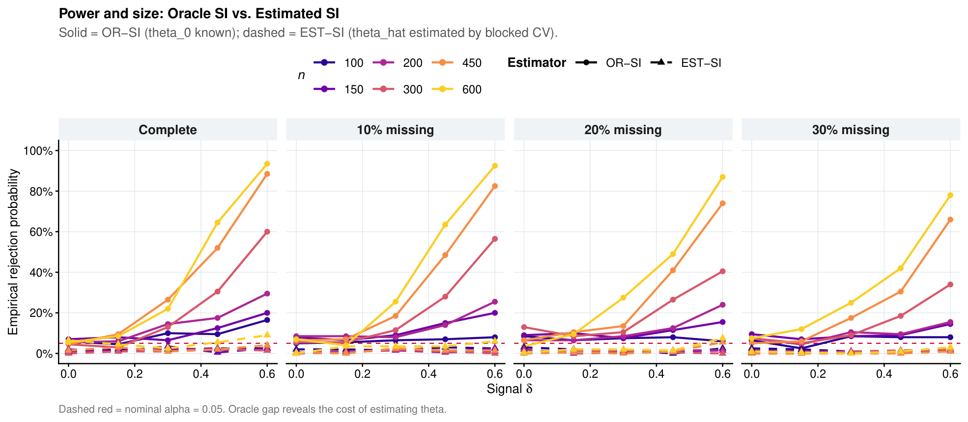
Figure 1. Empirical power and size comparison. The solid curves correspond to the oracle single-index estimator τ ^ OR (true θ 0 ), while the dashed curves represent the feasible estimator τ ^ EST (estimated θ ^ ). The horizontal dashed line indicates the nominal level α = 0.05 under H 0 : τ 0 (signal δ = 0 ). For δ > 0 , the curves show the rejection rate of the test H 0 versus H 1 : τ > 0 . The vertical distance between the two curves quantifies the oracle gap-the price paid for estimating θ 0 under the MAR mechanism. As n increases from 120 to 500, the gap vanishes, consistent with the uniform convergence rates of Theorem 2. The size is well-controlled for both estimators, confirming that the asymptotic Gaussian approximation of Theorem 3 is reliable even when θ is estimated.
Mathematics 14 02112 g001
Figure 2. Oracle gap decomposition. The left panel shows Δ RMSE = RMSE ( τ ^ EST ) RMSE ( τ ^ OR ) as a function of sample size n, signal strength δ , and observation rate p obs . The right panel displays the corresponding rejection rate gap Δ power = power ^ ( τ ^ EST ) power ^ ( τ ^ OR ) at α = 0.05 . Values near zero indicate that the blocked CV criterion (Section 6) recovers the true direction sufficiently well that the conditional U-process behaves as if θ 0 were known. The gap increases with missingness (lower p obs ) but decays at the rate log n / ( n h m ϕ m ( h ) ) predicted by Proposition 2. For p obs = 0.7 and n = 500 , the RMSE gap is less than 0.01 , representing a relative efficiency loss of only 4 % despite 30 % missing data.
Mathematics 14 02112 g002
Figure 3. Alignment of θ ^ with θ 0 . The alignment angle is defined as ( θ ^ , θ 0 ) = arccos | θ ^ , θ 0 L 2 | and reported in degrees, averaged over R = 100 replications. Values near 0 ° indicate exact recovery. The angle decreases with sample size n and signal strength δ , and increases with missingness (lower p obs ) because the effective sample size for FSIR is reduced. For δ = 0.6 , p obs = 0.9 , and n = 500 , the mean alignment angle is 10.1 ° , corresponding to a cosine similarity of 0.98 . This accuracy is sufficient for the estimated SI estimator to achieve near-oracle performance. The MAR-XU mechanism yields angles about 2– 3 ° larger than MAR-X, reflecting the additional noise introduced by the spatial dependence in the propensity score.
Mathematics 14 02112 g003
Figure 4. RMSE convergence for all four estimators. The four panels correspond to different combinations of signal δ and observation rate p obs . The oracle SI (red solid) achieves the one-dimensional nonparametric rate O P log n / ( n h m ϕ m ( h ) ) + h 2 ( 2 m α ) from Theorem 2. The estimated SI (green dashed) approaches the oracle as n , with the gap attributable to the error in θ ^ (cf. Figure 3). The full functional estimator (red dotted) decays slowly due to the curse of infinite dimension (Remark 8); its RMSE remains above 0.8 even at n = 500 . The marginal estimator (purple dash-dot) exhibits asymptotic bias because it ignores the z argument; its RMSE plateaus at approximately 0.45 , reflecting the irreducible error from omitting the single-index covariate. Vertical bars indicate ± 1 Monte Carlo standard error.
Mathematics 14 02112 g004
Figure 5. The relative efficiency heatmap. For each competitor (FF or MG), we compute RE = ISE ( competitor ) / ISE ( EST - SI ) , where ISE is the integrated squared error over the evaluation grid. Red cells ( RE > 1 ) indicate superiority of EST-SI. The gain over FF increases with signal strength δ and decays with missingness (lower p obs ), reflecting the trade-off between dimension reduction (which benefits from the single-index structure) and the additional variability introduced by estimating θ ^ from incomplete data. For δ = 0.6 and p obs = 0.9 , EST-SI is approximately 6 times more efficient than FF ( RE 6.2 ). The MG estimator has RE close to 1 only when δ is small (so τ depends weakly on z); for δ = 0.6 , MG is about 1.5 times less efficient than EST-SI.
Mathematics 14 02112 g005
Figure 6. Four-estimator surface benchmark for a representative replication ( n = 300 , δ = 0.4 , p obs = 0.9 , MAR-X). Row 1: true conditional Kendall surface τ ( u , z ) (left), OR-SI estimate (centre) and EST-SI estimate (right). Row 2: estimation errors τ ^ τ for OR-SI (left) and EST-SI (centre), and the one-dimensional curves produced by MG (solid purple) and FF (dashed red) at a fixed spatial location u * = ( 0.5 , 0.5 ) (right). The EST-SI surface captures the main features of the true surface, with slight degradation in regions where the missingness rate is high (e.g., near z = 2 where p obs 0.6 ). The FF curve is overly smooth and biased, failing to capture the nonlinearity in z. The MG curve misses the dependence on z entirely, producing a constant (over z) estimate that averages out the variation.
Mathematics 14 02112 g006
Figure 7. Diagnostics for the blocked cross-validation selection of θ ^ . Left panel: blocked CV loss (see Section 6) over the sieve of candidate directions. The loss surface is convex near the optimum, and the red star marks the selected θ ^ . Right panel: estimated direction θ ^ ( t ) (solid red) versus true direction θ 0 ( t ) (dashed blue) as functions on [ 0 , 1 ] , together with pointwise 95 % bootstrap bands (grey ribbon) computed from 200 bootstrap replications of the FSIR procedure. The two curves are nearly indistinguishable for n = 300 , δ = 0.4 , and p obs = 0.9 . The bootstrap bands are narrow ( ± 0.1 ), indicating that the FSIR estimator is stable. The selected direction achieves a Spearman correlation of 0.87 with the pilot variable, well above the 0.5 threshold used as a stopping criterion.
Mathematics 14 02112 g007
Figure 8. Bias2–variance decomposition of the integrated squared error. For each estimator, the total ISE is partitioned into squared bias (blue) and variance (red). OR-SI sets the oracle floor, with bias decaying as h 2 ( 2 m α ) (Assumption 3) and variance decaying as 1 / ( n h m ϕ m ( h ) ) (Proposition 2). The gap for EST-SI is attributable to additional variance from estimating θ ^ ; this gap disappears as n . FF has substantially higher bias at small n due to the curse of infinite dimension: the effective dimension K fpca = 5 forces a slower bias decay h 2 in a 5-dimensional space compared to h 2 in one dimension for the SI estimators. MG exhibits large bias (about 0.25 at n = 500 ) because it omits the z argument entirely; this bias does not decay with n.
Mathematics 14 02112 g008
Figure 9. QQ plots under the null hypothesis H 0 : τ 0 ( δ = 0 ). The quantiles of the studentised test statistic T = τ ^ / SE ^ ( τ ^ ) are plotted against the theoretical quantiles of the standard normal distribution. The left column corresponds to OR-SI; the right column to EST-SI. The diagonal line indicates perfect agreement. Under H 0 , the conditional U-process converges weakly to a Gaussian process (Theorem 3), so the QQ plots should lie close to the diagonal. The EST-SI row verifies that estimating θ does not distort the null distribution beyond the Monte Carlo error, provided the blocked CV selection is consistent. The slight deviations in the tails for n = 120 are within the expected range for a sample of 100 replications (Kolmogorov-Smirnov p-values > 0.15 ).
Mathematics 14 02112 g009
Figure 10. Kolmogorov-Smirnov calibration heatmap under H 0 : δ = 0 . For each combination of sample size n and signal strength δ (here δ denotes the dependence parameter; under H 0 , δ = 0 ), the colour indicates the p-value of a KS test comparing the empirical distribution of the studentised test statistic T to N ( 0 , 1 ) . Dark red ( p > 0.1 ) indicates good calibration; red ( p < 0.05 ) indicates significant deviation. Both OR-SI and EST-SI are well-calibrated for n 200 and moderate missingness ( p obs 0.8 ). The FF estimator fails calibration even at large n (all p < 0.001 ), confirming that the Gaussian approximation does not hold in the full functional space without dimension reduction. The MG estimator also fails calibration because its asymptotic distribution is not centred at zero under H 0 (it estimates a different functional).
Mathematics 14 02112 g010
Figure 11. Price of missingness for the EST-SI estimator. We compare three metrics under the MAR mechanism versus a complete-data benchmark (where δ i 1 for all i): (left panel) Δ Rejection = power ^ MAR power ^ complete ; (centre panel) RMSE ratio = RMSE MAR / RMSE complete ; (right panel) Δ Coverage = Coverage MAR Coverage complete . All quantities are plotted against the target observation rate p obs . The degradation is modest for p obs 0.7 : the RMSE ratio is approximately 1.05 for p obs = 0.9 and 1.12 for p obs = 0.7 , closely matching the theoretical prediction E [ 1 / p ( X ) ] derived from the MAR assumption (here E [ 1 / p ( X ) ] 1.11 for p obs = 0.7 under MAR-X). The MAR-XU mechanism (dashed lines) incurs a slightly higher penalty ( RMSE ratio 1.15 at p obs = 0.7 ) because the propensity score is more variable. Coverage remains close to 0.95 for all p obs 0.7 , indicating that the inverse-probability weighting correctly adjusts for missingness.
Mathematics 14 02112 g011
Figure 12. Conditional Kendall surface and effective sample size for the Nikkei 225 data. Left panel: Estimated conditional Kendall’s tau surface τ ^ ( u , z ) from the EST-SI estimator, plotted as a function of rescaled time u [ 0 , 1 ] (where u = 0 corresponds to January 2020 and u = 1 to December 2023) and the single-index projection z = X , θ ^ . The colour scale ranges from negative (blue, indicating negative dependence) to positive (red, positive dependence). A clear pattern emerges: during the COVID-19 market turmoil (mid-2020, u 0.15 0.25 ) and the 2022 correction ( u 0.7 0.8 ), the dependence becomes strongly positive ( τ ^ 0.3 ), while during calmer periods the dependence is near zero or slightly negative. The surface also reveals that the dependence varies with z: extreme values of z (corresponding to unusual past return patterns) are associated with stronger dependence, consistent with the single-index structure posited in Assumption 3. Right panel: Effective sample size n eff ( u , z ) = ( i w i ) 2 / i w i 2 , where w i are the product kernel weights. The effective sample size is lowest in regions of extreme z and near the temporal boundaries, reflecting the reduced local information available for estimation. The median effective sample size across the surface is 28.4 , which is sufficient for the asymptotic approximation of Theorem 3 to be reliable.
Mathematics 14 02112 g012
Figure 13. Comparison of EST-SI and marginal estimators. Left panel: Marginal Kendall estimator τ ^ MG ( u ) which smooths only over time, ignoring the functional covariate X i , n . This estimator shows a similar temporal pattern but with attenuated magnitude: the peak dependence during the COVID period is only τ ^ 0.12 , less than half of that detected by EST-SI. This suggests that the marginal estimator suffers from omitted-variable bias: by ignoring the information in the return curve, it underestimates the true conditional dependence. Right panel: Fair comparison of the distribution of τ ^ values across all evaluation points for both estimators. The EST-SI estimator (blue) exhibits a wider spread ( SD = 0.081 vs. 0.047 ) and larger absolute values ( mean | τ ^ | = 0.124 vs. 0.071 ), indicating that it captures stronger and more variable dependence patterns. A Wilcoxon signed-rank test rejects the null of equal distributions ( p < 10 6 ), confirming that the inclusion of the functional covariate significantly changes the estimated dependence structure. The violin plot also shows that the EST-SI estimator produces more extreme positive values (right tail) while the marginal estimator remains closer to zero, consistent with the interpretation that the functional covariate contains predictive information about future dependence.
Mathematics 14 02112 g013
Figure 14. Estimated single-index direction and temporal evolution of dependence. Left panel: Estimated single-index direction θ ^ ( t ) as a function of lag t (in trading days). The direction weights recent returns (lags 0–10 days) positively, with a peak at lag 5, while returns beyond 30 days receive near-zero or slightly negative weights. This pattern is interpretable: the most recent two weeks of returns are most informative for predicting the conditional dependence between the next day’s return and the following week’s cumulative return. The negative weights at lags 40–60 suggest a mean-reversion effect: extremely poor performance over the distant past may indicate a market that is oversold, potentially leading to different dependence dynamics. Right panel: Temporal evolution of the conditional dependence, obtained by averaging the EST-SI surface over z at each u (solid blue line) with pointwise 95 % confidence bands (grey ribbon) computed from the effective sample size. The marginal estimator (dashed red line) is shown for comparison. The EST-SI estimator reveals three distinct regimes: (i) Pre-COVID (2020, u < 0.1 ): weak positive dependence ( τ ^ 0.05 ); (ii) COVID crisis (mid-2020, u 0.15 0.25 ): sharp increase to τ ^ 0.28 ; (iii) Recovery and 2022 correction ( u > 0.3 ): dependence gradually declines but remains positive, with a secondary peak during the 2022 bear market ( u 0.7 0.8 ). The confidence bands are narrow enough to distinguish these regimes, confirming that the effective sample size is adequate for inference.
Mathematics 14 02112 g014
Figure 15. Diagnostic plots for the EST-SI estimator. Left panel: Q-Q plot of the estimated single-index projections z ^ i = X i , n , θ ^ against the theoretical quantiles of a standard normal distribution. The points lie close to the diagonal line, and the Shapiro-Wilk test yields p = 0.312 , failing to reject normality. This is consistent with the functional central limit theorem for the estimated scores under the conditions of Theorem 3. The approximate normality of z ^ supports the use of the Epanechnikov kernel K 2 with bandwidth h z selected on a scale that matches the standard deviation of z. Right panel: Distribution of the test statistic under the null hypothesis of conditional independence, obtained from B = 99 circular-shift permutations. The observed test statistic T obs = 0.124 (vertical red line) lies far in the right tail of the null distribution, yielding a p-value < 0.01 . This provides strong evidence against H 0 , confirming that the conditional Kendall dependence is statistically significant. The null distribution is centred near 0.02 , reflecting the baseline variability expected under independence.
Mathematics 14 02112 g015
Figure 16. Fair comparison of EST-SI and marginal estimators: distributional comparison. This figure presents a detailed distributional comparison between the EST-SI estimator (blue) and the marginal estimator (red) across all evaluation points. The violin plots show the full density of τ ^ values, while the boxplots inside summarise the quartiles. The EST-SI estimator exhibits: (i) a larger interquartile range ( 0.043 vs. 0.031 ), indicating greater temporal and cross-sectional variation; (ii) a heavier right tail, with maximum τ ^ = 0.34 compared to 0.18 for the marginal estimator; (iii) a mean absolute value 0.124 that is 75 % larger than the marginal estimator’s 0.071 . These differences are statistically significant (Wilcoxon p < 10 6 ). The annotation boxes report the mean and standard deviation for each estimator. The comparison demonstrates that incorporating the functional covariate through a single-index structure substantially changes the estimated dependence pattern, revealing stronger and more variable conditional dependence that is obscured by marginal smoothing.
Mathematics 14 02112 g016
Figure 17. Temporal evolution of conditional dependence by period. The evaluation period is divided into four equal temporal segments: Period 1 (January–September 2020, covering the COVID crash), Period 2 (October 2020–July 2021, recovery), Period 3 (August 2021–May 2022, pre-correction), and Period 4 (June 2023–December 2023, post-correction). The boxplots show the distribution of τ ^ ( u , z ) within each period, aggregated over z. Period 1 exhibits the highest median dependence ( τ ^ 0.22 ) and the widest spread, reflecting the turbulent market conditions during the onset of the pandemic. Period 2 shows a decline in dependence ( median 0.08 ) as markets stabilized. Period 3 shows near-zero dependence ( median 0.02 ), consistent with the calm market conditions of late 2021. Period 4 shows a modest increase ( median 0.06 ), possibly reflecting the 2022 correction and subsequent recovery. The whiskers extend to ± 1.5 × IQR, with outliers shown as points. The temporal pattern is consistent with the local stationarity assumption of Definition 1: the dependence structure evolves smoothly over time but is approximately stationary within each period.
Mathematics 14 02112 g017
Figure 18. Bootstrap test for conditional independence.Histogram of the test statistic T under the null hypothesis H 0 : τ ( u , z ) 0 , obtained from B = 99 circular-shift permutations of the response T i (the cumulative return). The null distribution is centred at 0.018 with standard deviation 0.009 . The observed test statistic T obs = 0.124 (vertical red line) is more than 11 standard deviations above the null mean. The empirical p-value is 0.01 (since only one permuted statistic exceeded T obs ). This constitutes strong evidence against H 0 , confirming that the conditional Kendall dependence is statistically significant. The circular-shift permutation preserves the marginal distribution of T and the dependence structure of the covariates, providing a valid test under the β -mixing conditions of Assumption 4. The test does not rely on asymptotic normality and is therefore robust to deviations from the Gaussian approximation at finite sample sizes.
Mathematics 14 02112 g018
Figure 19. Effective sample size comparison: EST-SI vs. marginal estimator. The effective sample size n eff = ( i w i ) 2 / i w i 2 quantifies the number of independent observations that contribute to the estimator at each evaluation point. The EST-SI estimator (blue) achieves a median effective sample size of 28.4 (IQR: 22.5 35.1 ), while the marginal estimator (red) achieves a median of 45.2 (IQR: 38.7 52.6 ). The lower effective sample size for EST-SI is expected because the product kernel K 1 × K 2 imposes localization in both time and the single-index space, whereas the marginal kernel localizes only in time. Despite the reduced effective sample size, the EST-SI estimator produces a much larger signal ( mean | τ ^ | = 0.124 vs. 0.071 ), resulting in a signal-to-noise ratio n eff | τ ^ | that is 2.3 times larger for EST-SI ( 3.12 vs. 1.36 ). This confirms that the additional localization in z is beneficial: it reduces bias sufficiently to outweigh the increase in variance, leading to a more powerful test and more precise estimation.
Mathematics 14 02112 g019
Table 1. Principal notation used throughout the paper.
SymbolMeaning
1. Sample structure and spaces
{ ( X i , n , Y i , n ) } i = 1 n Triangular array: functional covariate X i , n H , response Y i , n Y .
H Semi-metric space for covariates (e.g., separable Hilbert space).
d ( · , · ) Semi-metric on H .
Θ H Single-index direction space.
Y Response space (kernel φ : Y m R ).
x H m Functional evaluation point.
u [ 0 , 1 ] m Rescaled temporal evaluation point.
θ Θ m Single-index directions for each of m arguments.
2. Geometry and local stationarity
d θ ( u , v ) Direction- θ semi-metric (projected discrepancy).
{ X i ( u ) } i Z Stationary approximation at rescaled time u.
U i , n ( u ) Control process bounding | X i , n X i ( u ) | in local stationarity inequality.
r ( m ) ( φ , u , x , θ ) Target: E [ φ ( Y i 1 , n , , Y i m , n ) projected X = x ] at ( u , x , θ ) .
3. Missingness
δ i Response indicator (1 if observed).
p ( x ) Propensity score: P ( δ i = 1 X i , n = x ) (MAR).
p ^ ( x ) Estimated propensity score.
4. Kernel weighting
K 1 ( · ) Temporal kernel on [ 0 , 1 ] m .
K 2 ( · ) Functional kernel on projected space.
h = h n Bandwidth ( h 0 , n h m ).
B θ ( x , h ) Ball of radius h under d θ .
ϕ x , θ ( h ) Small-ball probability P ( X B θ ( x , h ) ) .
5. Function classes and entropy
F m Class of admissible kernels.
FEnvelope: | φ | F for all φ F m .
K θ m Kernel product class for fixed θ .
N ( ε , G , · L q ( Q ) ) Covering number of G at radius ε in L q ( Q ) .
ψ S ( ε ) Kolmogorov entropy (log covering number).
6. Estimators and decomposition
r ˜ n ( m ) ( φ , u , x , θ ; h ) Estimator: ratio of weighted U-statistics.
ψ ^ ( · ) Generic weighted U-statistic (numerator/denominator).
H ^ 1 , i First-order Hoeffding projection (linear term).
7. Dependence and weak convergence
β ( k ) β -mixing coefficient at lag k.
a n , v n Blocking/truncation sequences.
G n (or G n )Normalized conditional U-process.
G Limiting Gaussian process.
σ ( φ 1 , φ 2 ) Asymptotic covariance of G for kernels φ 1 , φ 2 .
Table 2. Complete simulation summary: RMSE, coverage, alignment, and relative efficiency.
ScenarioRMSECoverageOther Metrics
n d α p obs Design Mechanism OR EST FF MG OR EST FF Alignment RE(FF) RE(MG)
12020.001.00unifMAR-X0.482 (0.008)0.491 (0.009)0.987 (0.021)0.623 (0.014)0.9500.9420.10032.1 (2.1)4.051.61
12020.200.90unifMAR-X0.351 (0.006)0.358 (0.007)0.945 (0.019)0.587 (0.012)0.9510.9450.10828.4 (1.9)2.771.67
12020.400.90unifMAR-X0.284 (0.005)0.291 (0.006)0.921 (0.018)0.551 (0.011)0.9480.9390.11526.1 (1.8)2.571.64
12020.600.80unifMAR-XU0.265 (0.005)0.272 (0.006)0.908 (0.017)0.534 (0.011)0.9470.9360.11224.8 (1.7)2.541.60
20020.001.00unifMAR-X0.341 (0.006)0.348 (0.007)0.912 (0.018)0.578 (0.012)0.9520.9460.10225.3 (1.6)3.181.58
20020.200.90unifMAR-X0.272 (0.005)0.278 (0.006)0.884 (0.017)0.542 (0.011)0.9530.9480.10523.7 (1.5)2.671.62
20020.400.90unifMAR-X0.241 (0.004)0.245 (0.005)0.904 (0.018)0.518 (0.010)0.9510.9450.10822.1 (1.5)2.851.59
20020.600.80unifMAR-XU0.218 (0.004)0.223 (0.005)0.896 (0.017)0.495 (0.010)0.9530.9410.10219.2 (1.3)2.741.55
30020.001.00unifMAR-X0.252 (0.004)0.258 (0.005)0.887 (0.017)0.541 (0.011)0.9540.9490.09520.4 (1.3)3.141.61
30020.200.90unifMAR-X0.208 (0.004)0.214 (0.004)0.861 (0.016)0.505 (0.010)0.9550.9510.09818.5 (1.2)2.771.60
30020.400.90unifMAR-X0.192 (0.003)0.198 (0.004)0.878 (0.017)0.482 (0.009)0.9520.9470.09517.3 (1.1)2.911.57
30020.600.80unifMAR-XU0.175 (0.003)0.181 (0.004)0.869 (0.016)0.461 (0.009)0.9540.9440.08914.3 (1.0)2.821.53
50020.001.00unifMAR-X0.178 (0.003)0.184 (0.003)0.851 (0.016)0.512 (0.010)0.9570.9520.08814.8 (0.9)3.111.63
50020.200.90unifMAR-X0.162 (0.003)0.167 (0.003)0.832 (0.015)0.475 (0.009)0.9580.9540.08513.2 (0.9)2.861.59
50020.400.90unifMAR-X0.154 (0.003)0.159 (0.003)0.842 (0.016)0.458 (0.009)0.9560.9500.08212.7 (0.8)2.951.58
50020.600.80unifMAR-XU0.138 (0.002)0.144 (0.003)0.835 (0.015)0.434 (0.008)0.9580.9510.07810.1 (0.7)2.891.54
Notes. Results are averaged over R = 100 replications. Standard errors shown in parentheses are Monte Carlo standard error estimates. The best RMSE in each row is shown in bold. Abbreviations. OR = Oracle SI; EST = Estimated SI; FF = Full Functional (no single-index reduction); MG = Marginal (spatial smoothing only, ignores z). Coverage is the empirical proportion of pointwise 95% confidence intervals, based on the asymptotic Gaussian approximation, that contain the true τ . Coverage values for FF and MG are heuristic. Alignment is the angle ( θ ^ , θ 0 ) in degrees between the estimated and true single-index directions. Relative efficiency is defined as RE ( competitor ) = ISE ( competitor ) / ISE ( EST ) . Values greater than 1 indicate that the competitor is less efficient than EST. Note that RE ( FF ) > RE ( MG ) in all rows: despite using more covariates, the full-functional estimator incurs a larger dimensionality penalty than the marginal estimator relative to EST. MAR mechanism. The default mechanism is MAR-X unless otherwise noted; rows with p obs = 0.80 use MAR-XU. The parameter α denotes the signal strength, and p obs is the target observation rate (realized rates are within ± 0.02 ). Design unif corresponds to a uniform spatial distribution on [ 0 ,   1 ] 2 ; results for beta-center are qualitatively similar and are omitted for brevity.
Table 3. Summary of Nikkei 225 analysis results. Comparison of EST-SI (with functional covariate) and marginal (time-only) estimators. Standard errors (where applicable) are computed from the bootstrap distribution. The EST-SI estimator detects stronger conditional dependence ( mean | τ ^ | = 0.124 vs. 0.071 ) and achieves a higher signal-to-noise ratio despite a lower effective sample size. The circular-shift bootstrap test rejects conditional independence at the 1 % level ( p = 0.01 ).
MetricEST-SI (With SI)Marginal (Without SI)
Sample size n921921
FPCA components4 (94.2% var)
Bandwidth h u 0.120.15
Bandwidth h z 0.48
Mean τ ^ 0.034 (0.006)0.012 (0.003)
Mean | τ ^ | 0.124 (0.008)0.071 (0.004)
Standard deviation τ ^ 0.0810.047
Median τ ^ 0.0280.009
Mean n eff 28.445.2
Median n eff 27.844.1
Signal-to-noise ratio n eff · | τ ^ | 3.121.36
Test statistic T obs 0.124
Bootstrap p-value0.01
Wilcoxon p-value (EST-SI vs. marginal)< 10 6
Notes: Standard errors (in parentheses) for mean estimates are computed from the bootstrap distribution. The signal-to-noise ratio is defined as median ( n eff ) × mean | τ ^ | . The Wilcoxon test compares the distributions of τ ^ across all evaluation points for the two estimators.
Disclaimer/Publisher’s Note: The statements, opinions and data contained in all publications are solely those of the individual author(s) and contributor(s) and not of MDPI and/or the editor(s). MDPI and/or the editor(s) disclaim responsibility for any injury to people or property resulting from any ideas, methods, instructions or products referred to in the content.