Article

Sparse Simulation of Autoregressive Gaussian Processes

1
Jožef Stefan Institute, Jamova cesta 39, 1000 Ljubljana, Slovenia
2
Centre for Information Technologies and Applied Mathematics, University of Nova Gorica, 5000 Nova Gorica, Slovenia
*
Author to whom correspondence should be addressed.
Mathematics 2026, 14(12), 2111; https://doi.org/10.3390/math14122111
Submission received: 4 May 2026 / Revised: 1 June 2026 / Accepted: 11 June 2026 / Published: 13 June 2026
(This article belongs to the Special Issue Nonlinear Dynamics and Control: Challenges and Innovations)

Abstract

This study proposes a novel and improved numerical approximation of the simulation of Gaussian process autoregressive models. As a Bayesian nonparametric regression method, Gaussian process models offer the unique advantage of providing closed-form uncertainty quantification. When Gaussian process models are used for autoregressive models, the validation procedure requires the model’s simulation or multi-step-ahead prediction. However, simulating dynamical Gaussian process models is complex due to the intractable propagation of uncertain inputs through the nonlinear model. Numerical approximation, namely Monte Carlo simulation, is one of the most frequent options for simulating dynamical models based on Gaussian processes. The computational burden of Monte Carlo simulation algorithms increases cubically with data size, representing a challenge. This paper introduces a unified simulation framework invariant to sparse and variational approximations to obtain a static sample from the pseudo-point posterior. Furthermore, we propose an innovative method for simulating Gaussian process dynamical models. A single parameter is proposed to regulate the trade-off between computational complexity and algorithmic accuracy. This innovation demonstrates the potential to replace the conditionally independent Monte Carlo method with no additional computational burden, thereby enhancing estimates of latent responses. The proposed simulation method is demonstrated using two synthetic examples and a realistic case study.

1. Introduction

The following investigation proposes improved numerical approximations of the simulation of Gaussian-process (GP) autoregressive models.
GP models deliver a well-calibrated predictive distribution at a model output, providing a systematic quantification of model fidelity [1]. This characteristic makes them particularly suitable for applications where a nuanced understanding of model uncertainty is crucial, such as in safety-critical scenarios [2], robust control systems [3], and fault detection. GPs, characterised by their utilisation of an infinite number of basis functions [4,5,6,7], belong to a class of probabilistic models. Leveraging a nonparametric structure, GPs effectively reduce the number of metaparameters and seamlessly scale model complexity with the size of the dataset. The model’s ability to penalise overly complex structures is inherently embedded in the evidence [8].
While closed-form calculations are available for both the marginal and conditional distributions, the associated algorithm exhibits cubic computational complexity and quadratic memory complexity [9]. One systematic approach for reducing computational complexity involves employing sparse approximation methods, where a reduced set of pseudo-points, denoted by m < n , summarises the data [10,11,12].
Among the various sparse-based approximations of the prior distribution, the Fully Independent Training Conditional (FITC) method is one of the most popular. FITC involves a joint optimisation of pseudo-points and hyperparameters through gradient-based optimisation strategies [13].
A more recent extension of sparse approximations involves a direct approximation of the posterior using variational inference without imposing additional assumptions about the prior. Pseudo-inputs and hyperparameters are obtained by maximising the lower bound of the actual Marginal Log-Likelihood (MLL), a process equivalent to minimising the Kullback–Leibler (KL) divergence between the true and the approximated posterior. This approach rigorously defines the distance between the true and the approximated posterior. The parameters of the free variational distribution can be treated as model parameters, giving rise to a Scalable Variational Gaussian Process (SVGP) [14,15,16].
SVGP facilitates stochastic optimisation and provides an unbiased estimation of the lower bound of the true MLL from random subsets of training data. An alternative is deriving a collapsed bound, wherein the optimal parameters of the free variational distribution are analytically determined, resulting in a Variational Free Energy (VFE) approximation [17]. However, this reintroduces the full correlation between data points, making the bound unsuitable for stochastic optimisation.
While initially conceived, approximations were for static systems; many of these concepts seamlessly extend to dynamical models. A natural adaptation involves a direct functional relationship between time and output observations within a dynamical model, with the mapping captured by a GP. However, this type of static regression cannot inherently learn the system’s dynamics. A viable approach to addressing this involves representing the system’s dynamics through a Finite Impulse Response (FIR) model. In this model, the current output observation depends upon a finite set of lagged exogenous variables [18]. An inherent challenge with FIR models lies in the necessity to select a relatively large order, corresponding to the number of lagged exogenous inputs [19]. Alternatively, one may consider an Infinite Impulse Response (IIR) model, where a functional relationship between the current output observation and all past exogenous variables encapsulates the system’s dynamics.
The introduction of lagged-output observations as additional inputs forms a nonlinear autoregressive model with exogenous inputs (NARX).
The orders of NARX models required to achieve comparable accuracy are notably smaller than those of FIR models. This makes NARX models using GPs, namely GP-NARX combinations, more suitable for real-world applications.
The elegance of the NARX model lies in its simplification of model training to that of the static case. This characteristic renders the NARX model particularly advantageous for scalability to large datasets, simplifying experimentation and offering practical advantages over more specialised models. Notably, the NARX approach can surpass the performance of alternative models, such as state-space models (GP-SSM) [20,21,22,23] or nonlinear output-error models (GP-NOE) [24]. The versatility and robustness of the NARX model make it a compelling choice for a wide range of applications, and this study focuses on these.
A particular case of the multiple-step-ahead prediction is the simulation, where the prediction horizon is infinite [6], or in practice, sufficiently large. There are two primary motivations for conducting simulations:
  • Forecasting future system states: Simulations enable the anticipation of the system’s state over an extended prediction horizon, allowing insights into its behaviour over multiple future steps;
  • Model validation for dynamical systems: Simulations are crucial for validating the dynamical system model. This validation is particularly noteworthy in NARX models, as it assesses model performance in an operational regime for which the model was not explicitly trained.
While the first point underscores the intuitive need for predicting future states [25], the second point highlights the unique aspect of NARX models, where model performance is rigorously evaluated in real-world operating conditions that were not part of the model training data. A successful simulation accurately describes observations and validates the assumptions embedded in the model under practical circumstances.
GP-NARX models are favoured for straightforward training procedures, yet the simulation process necessitates an iterative approach. During simulation, predictions from previous timesteps are utilised as inputs for subsequent timesteps, extending indefinitely or until the conclusion of the prediction horizon. However, this introduces uncertainty into the inputs and the need for approximations [26,27,28,29,30]. A significant challenge in dynamical GP-NARX models arises from the propagation of uncertainty—as distributions of random variables at model input can be interpreted—through nonlinear models, which is intractable [31,32,33]. The propagation of uncertainty extends beyond training, presenting complexities in multi-step-ahead predictions. In GP-NARX models, the Gaussian distribution undergoes sequential propagation through the nonlinear model, resulting in an analytically intractable problem [6].
The approximated simulation procedures in GP-NARX models can be broadly categorised into three types:
  • Naïve simulation: This method propagates the mean of the prediction, resulting in an underestimation of the forecasted uncertainty [6];
  • Approximations of statistical moments: This category further subdivides into two approaches—those employing a Taylor expansion [29] and those employing exact matching of statistical moments [27,34]. Unfortunately, the former is considered a rough approximation. At the same time, the latter only applies to a limited set of covariance functions, such as the squared exponential function and a linear function [6]. An inherent drawback of methods based on the approximation of statistical moments is their neglect of higher statistical moments.
  • Numerical approximations: This approach involves employing numerical techniques, i.e., the Monte Carlo (MC) method, to sample simulated trajectories [21,35,36,37];
Given the increasing computational capabilities, numerical approximations utilising MC sampling have gained prominence. MC-based simulation offers the advantage of not constraining the model to a specific choice of covariance function, enabling the identification of higher statistical moments.
Unfortunately, the existing work on improving the scalability of GP models does not translate well to MC sampling of trajectories in dynamical GP models. The MC approach exhibits cubic computational complexity with the number of predicted steps into the future [21]. When implementing an MC sampler for GP-NARX trajectories, the Gaussian distribution extends to all function evaluations, necessitating storing consecutive MC samples in memory. This substantially increases the computational complexity, especially for long prediction horizons in GP-NARX models [37].
A commonly adopted strategy to mitigate computational complexity during simulation involves assuming conditional independence between consecutive latent values, given those associated with the training data. While this assumption introduces a rough simplification that is mathematically imprecise, it does offer a significant reduction of computational complexity [38]. Nevertheless, the assumption of conditional independence may not hold in all practical scenarios, potentially leading to inaccuracies in the simulation results. Our challenge in this investigation is getting less computational complexity and acceptable memory requirements at acceptable accuracy.
The main contribution presented is twofold.
  • This study, which is based on the thesis [39], proposes a unified and original framework for numerically simulating GP-NARX models, drawing inspiration from the static representation introduced in [40]. Our approach divides the simulation algorithm into a GP-specific static part and a dynamical part that remains consistent across various sparse approximations.
  • A novel approximation named Thresholded Correlated Monte Carlo (TCMC) simulation that advances the state-of-the-art in GP simulation of dynamical systems is introduced, contributing the following advancements:
    (a)
    An approximated MC-based simulation algorithm featuring a single parameter that balances the trade-off between the computational complexity and the accuracy of the simulation approximation, which can, in the limit, recover the ground truth.
    (b)
    Special case of the proposed simulation approximation, Pseudo Independent Monte Carlo (PIMC) simulation, enhances estimated simulations’ accuracy while maintaining the same computational complexity as the existing Conditionally Independent MC simulation [38].
    (c)
    Development of compact and efficient simulation algorithms applicable to sparse and variational approximations. An open-source GP-NARX model training and simulation toolbox is also available, accessible at the following repository: https://github.com/tadejkrivec/GPflow-NARX (accessed on 10 June 2026).
This paper is organised as follows: In Section 2, we provide an in-depth introduction to GP-NARX models and their popular sparse and variational approximations. We establish a unified representation for predictions across these approximations, creating a crucial bridge toward developing a unified simulation algorithm. The section ends with the presentation of the unified simulation procedure. In Section 3, we list MC approximations to the unified GP-NARX model simulations. Section 4 introduces the novel approximation method for simulating GP-NARX models. This section explores a particular case of the approximation, demonstrating its capacity to significantly enhance independent MC simulations without incurring additional computational costs while ensuring a more accurate approximation to the ground truth. Section 5 systematically compares the proposed approximations through two synthetic illustrative examples and a realistic case study, namely a dynamical benchmark problem, highlighting the problematic training and test data size for conventional GP-NARX models. Section 6 briefly summarises the contributions and concludes with some final remarks.

2. Methodology

2.1. Vanilla GP-NARX Model

We assume the true dynamics satisfy
f t = f f t n a , , f t 1 , x t n b , , x t 1 ,
where f is a nonlinear function, f t is the function evaluation at timestep t, x are the exogenous variables, and  n a , n b > 0 denote the number of lags for the delayed latent values and delayed exogenous variables, respectively. Equivalently, in matrix form,
f 1 : t = f ( Z 1 : t ) ,
where f 1 : t is the vector of latent function values and Z 1 : t R t × ( n a + n b ) is the NARX input matrix (t observations). The i-th row of Z 1 : t is
z i T = [ f i n a , , f i 1 , x i n b , , x i 1 ] .
Because the latent variables are not attainable in practice, we instead observe a noisy output vector, y 1 : t = f 1 : t + ϵ , with  ϵ N ( ϵ | 0 , I σ n 2 ) . While alternative observation models are possible, this additive assumption is the most common presumption [5,6].
The dynamical system is thus written as
y 1 : t = f ( Z 1 : t ) + ϵ ,
where the i-th row of Z 1 : t is now defined using the noisy outputs,
z i T = [ y i n a , , y i 1 , x i n b , , x i 1 ] .
Our goal is to infer the latent function f in Equation (4). Here, we focus on the case where f is modelled with a GP [5].
A GP is a collection of random variables such that any finite subset has a joint Gaussian distribution. It is fully characterised by its mean m · and covariance function k · , · ,
m z = E [ f ( z ) ] ,
k z , z = E [ ( f ( z ) m ( z ) ) ( f ( z ) m ( z ) T ) ] .
We write the GP prior as
f · GP f · | m · , k · , · ,
where m · and k · , · are parametrised by hyperparameters θ . Using Bayes’ theorem, the prior over functions is transformed into the posterior,
GP f · | y 1 : t , θ , σ n 2 = p y 1 : t | f 1 : t , σ n 2 GP f · | θ p y 1 : t | θ , σ n 2 ,
where the likelihood p y 1 : t | f 1 : t , σ n 2 is assumed Gaussian. For notational simplicity, the conditioning on the choice of m · and k · , · in Equation (8) is replaced by θ . We will typically omit conditioning on θ and σ n 2 , since these are usually deterministic variables learned from data, and reintroduce them only when they are parameters of interest or random variables. Without loss of generality, we henceforth assume m · = 0 .
In practice, we work with finite sets of random variables and marginalise out latent quantities that are not of interest,
p f 1 : t + n = GP f · d f { f 1 : t + n } ,
p f 1 : t + n | y 1 : t = GP f · | y 1 : t d f { f 1 : t + n } ,
where f { f 1 : t + n } is the set of all latent values outside { f 1 : t + n } . Note that { f 1 : t + n } = { f 1 : t , f t + 1 : t + n } , where f 1 : t corresponds to the observations and f t + 1 : t + n are the desired latent values up to n steps into the future. The marginalisation property of Gaussian distributions allows all remaining latent variables to be ignored; see [5] for details.
Unfortunately, vanilla GP-NARX models scale cubically with the training data size. Accordingly, the dominant practical obstacles in training and simulating dynamical GPs are computational complexity and memory requirements. The sparse approximation methods reviewed next are introduced to reduce computational complexity.

2.2. Sparse GP-NARX Model

Sparse approximations aim to identify a representative set of m pseudo-inputs that summarise the data well [10]. This can be interpreted as a form of dimensionality reduction, but in the row space of the input matrix (data points) rather than its column space (features). We introduce m pseudo-inputs
z 1 : m = [ z 1 , , z m ]
and the associated latent function values
u = [ u 1 , , u m ] ,
which are drawn from the same joint distribution as f 1 : t + n . This construction mirrors the vanilla GP, where pseudo-points u are implicitly present but marginalised out.
Computational savings arise once we assume f 1 : t and f t + 1 : t + n are conditionally independent given u , yielding the approximate joint prior
p ( f 1 : t + n ) p ( f 1 : t | u ) p ( f t + 1 : t + n | u ) p ( u ) d u .
The joint Gaussian distribution is fully determined by the conditional distributions given the pseudo-points,
p ( f 1 : t | u ) = N ( f 1 : t | K f 1 : t , u K u , u 1 u ,
K f 1 : t , f 1 : t Q f 1 : t , f 1 : t )
p ( f t + 1 : t + n | u ) = N ( f t + 1 : t + n | K f t + 1 : t + n , u K u , u 1 u ,
K f t + 1 : t + n , f t + 1 : t + n Q f t + 1 : t + n , f t + 1 : t + n ) ,
where Q a b = K a , u K u , u 1 K u , b . As in the vanilla GP-NARX case, the posterior is obtained via
p ( f 1 : t + n | y 1 : t ) = p y 1 : t | f 1 : t p ( f 1 : t + n ) p y 1 : t ,
with p ( f 1 : t + n ) defined by Equation (12).
The conditional-independence assumption in Equation (12) alone is still insufficient for practical computational improvements, so additional structure is typically imposed. In this work, we consider two widely used approaches:
  • Prior approximations;
  • Posterior approximations.
A comparison of the prior and posterior approximations can be found in [11]. The Fully Independent Training Conditional (FITC) approximation is a prior approximation. It keeps the test conditional p ( f t + 1 : t + n | u ) exact, but replaces the training conditional with
p ( f 1 : t | u ) q ( f 1 : t | u ) = i = 1 t p ( f i | u ) .
Variational approximations, in contrast, approximate the posterior directly and therefore belong to posterior approximations. We introduce a free variational distribution q ( u ) = N ( u | m , Φ ) and obtain the lower bound
p y 1 : t | θ , σ n 2 L ( m , Φ , z 1 : m , θ , σ n 2 )
= E q ( f 1 : t ) [ log p ( y 1 : t | f 1 : t ) ] KL [ q ( u ) | | p ( u ) ] ,
where m and Φ parameterise the free variational distribution. By lower-bounding the MLL, the free variational distribution is encouraged towards the exact posterior over the pseudo-points, i.e.,  q u p u | y 1 : t [17,41].
The most scalable sparse method considered here is the Scalable Variational Gaussian Process (SVGP) [14,15], where the variational distribution remains free and is learned by stochastically optimising the Evidence Lower Bound (ELBO) [14]. We refer to this approximation as the GP-NARX (SVGP) model. The less scalable alternative is the Variational Free Energy (VFE) method: its key benefit is that the variational distribution is determined optimally by maximising the ELBO in closed form. However, this reintroduces correlations between data points and prevents stochastic optimisation. We refer to this approximation as the GP-NARX (VFE) model.

2.3. Unified Prediction in GP-NARX Models

This paper does not focus on learning the model parameters (i.e., θ , σ n 2 ). We therefore assume they are given and fixed; a description of model learning is provided in Appendix D.
Given learned parameters, the objective is to predict the model output at the next timestep t + 1 . The presentation below follows [10,11,16], to which we refer for full derivations and discussion. Starting from Equation (9b), prediction is obtained by marginalising the training latent function values f 1 : t . A unified description covering the vanilla GP and the sparse approximations is [10,11,16]
q ( f t + 1 ) = p ( f 1 : t + n | y 1 : t ) d f { f t + 1 } p ( f t + 1 : t + n | u ) p ( f 1 : t | y 1 : t , u ) q ( u ) d u d f { f t + 1 } p ( f t + 1 | u ) q ( u ) d u ,
where the distribution q ( u ) depends on the chosen approximation,
q ( u ) = p ( f 1 : t | y 1 : t ) Vanilla GP-NARX , defined by Equation ( A 18 ) , q ( u ) = p ( u | y 1 : t ) GP-NARX ( FITC ) , defined by Equation ( A 19 ) , q ( u ) p ( u | y 1 : t ) GP-NARX ( VFE ) defined by Equation ( A 21 ) , q ( u ) p ( u | y 1 : t ) GP-NARX ( SVGP ) , defined by Equation ( A 22 ) ,
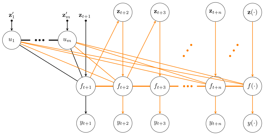
where the letter in the equation labels indicates that the corresponding expressions are collected in the Appendix G. In particular, vanilla GP-NARX prediction is recovered when q ( u ) is taken as the posterior over the training latent function values. In Figure 1, the prediction mechanism corresponds to the black interconnected part. The final integral in Equation (17) is analytically tractable; each approximation leads to a different closed-form expression. The resulting predictions are summarised in Appendix G.

2.4. Unified Simulation in GP-NARX Models

To enable a streamlined simulation algorithm, we retain the explicit form of q ( u ) rather than analytically marginalising it. Although this choice offers limited benefit for prediction, it allows the simulation procedure to be separated into two components:
  • Static part: Approximation-specific, with readily available algorithms and implementations.
  • Dynamical part: Shared across the approximations considered here, enabling reuse of the same dynamical simulation code.
The decomposition into static and dynamical components separates the closed-form posterior prediction from the recursive simulation problem. The static component contains approximation-specific posterior predictive distributions, while the dynamical component describes the recursive evolution of the simulated trajectory. This separation enables a unified simulation framework across multiple sparse GP approximations.
If the final step in Equation (17) is marginalised, each approximation yields a different simulation algorithm, which obstructs a generalised implementation. Moreover, because latent function values up to timestamp t + n depend on the propagation of random inputs through a nonlinear transformation, closed-form solutions are unavailable; consequently, the final integral in Equation (17) must be estimated numerically. The same numerical methodology then applies to later steps.
The unified simulation of latent function values is defined as
q ( f t + 1 : t + n ) = i = 2 n p ( f t + i | f t + 1 : t + i 1 , u ) q ( u ) d u ,
where q ( u ) is the static part and i = 2 n p ( f t + i | f t + 1 : t + i 1 , u ) is the dynamical part. For an arbitrary parameter value n a , the dynamical part up to timestamp t + n can be written as
p ( f t + i | f t + 1 : t + i 1 , u ) = p ( f t + 2 n a : t + 1 | u ) · ( i = 2 n p ( f t + i | f t + 1 : t + i 1 , u , z t + i ) · p ( z t + i | f t + i n a : t + i 1 ) d z t + i ) d f { f t + 1 : t + i }
where
p ( z t + i T | f t + i n a : t + i 1 )           = δ z t + i T [ f t + i n a : t + i 1 T , x t + i n b : t + i 1 T ] ,
with δ denoting the Dirac delta, indicating that the autoregressive input is constructed deterministically from the known lagged latent values.
Because GP-NARX models are not trained sequentially in the output-error sense, a conservative alternative is to propagate noisy values through the inputs,
p ( z t + i T | y t + i n a : t + i 1 )           = δ z t + i T [ y t + i n a : t + i 1 T , x t + i n b : t + i 1 T ] ,
where y t + i n a : t + i 1 p ( y t + i n a : t + i 1 | f t + i n a : t + i 1 ) . This choice can be motivated by the use of noisy observations in the definition of input regressors in GP-NARX models. However, because training emphasises step-ahead prediction, there is no definitive criterion that uniformly favours one propagation strategy. If the error-in-variables effect is negligible, latent propagation in the output-error sense may be preferable; if it is substantial, propagating noisy values may be more appropriate. In practice, the better option is determined empirically (e.g., via cross-validation). Unless stated otherwise, we adopt the latent—output-error—approach.
The simulation is obtained by sequential MC sampling. A k-th sequential sample unrolls through the chained Gaussian distributions,
draw u ˜ k q ( u ) ,
draw f ˜ t + 2 n a : t + 1 k p ( f t + 2 n a : t + 1 | u ˜ k ) ,
draw z ˜ t + 2 k p ( z t + 2 | f ˜ t + 2 n a : t + 1 k ) ,
draw f ˜ t + 2 k p ( f t + 2 | f ˜ t + 1 k , u ˜ k , z ˜ t + 2 k ) ,
draw z ˜ t + n k p ( z t + n | f ˜ t + n n a : t + n 1 k ) ,
draw f ˜ t + n k p ( f t + n | f ˜ t + 1 : t + n 1 k , u ˜ k , z ˜ t + n k ) .
Noisy values can then be drawn independently,
draw y ˜ t + 1 : t + n k p y t + 1 : t + n | f ˜ t + 1 : t + n k .
Posterior marginals, which can be interpreted as a Gaussian Mixture Model (GMM) [42] at an arbitrary timestep t + i , are approximated by
q ( f t + i ) 1 r k = 1 r p ( f t + i | f ˜ t + 1 : t + i 1 k , u ˜ k , z ˜ t + i k ) ,
where r denotes the number of MC samples. At each step, the latent distribution can be represented as a GMM. Overall, the unified simulation can be interpreted as a two-part procedure:
  • Batch sample latent function values with known inputs before the simulation begins (approximation-specific but static);
  • Iteratively sample the remaining quantities conditioned on the static latent function values (shared across approximations but dynamic).
Figure 1 provides a PGM of the unified simulation.
Finally, note that the distribution over u is approximation-specific. The black interconnected part of the graphical model is static and supports a straightforward batch sampling procedure. The orange interconnected part is the dynamical component; algorithmically, it is consistent across all approximations once the pseudo-input realisations are fixed.

3. Existing Approximations to the Unified GP-NARX Model Simulation

As presented in the previous section, the unified representation of the GP-NARX model simulation opens avenues for novel approximations within the simulation algorithm that are universally applicable across diverse GP-NARX models. Before introducing a novel approximation to the simulation’s shared dynamical aspect, we explain in this section the existing approximations in the context of the presented simulation. A summary of existing numerical simulation methods is necessary for the subsequent exposition.

3.1. Fully Correlated Monte Carlo (FCMC) Simulation

We start with an FCMC simulation [37], as the conventional numerical simulation method for the simulation of dynamical GP models. The latent distribution at an arbitrary timestep t + i for FCMC is defined by Equation (A23), where the letter in the equation label means that this equation can be found in the Appendix H.1, which is exact for q u = p u | y 1 : t . This is a fully correlated simulation and enables an arbitrarily good approximation of the posterior if we disregard the numerical complexity with an increasing number of samples. Consequently, we will compare the results of other methods to the results of FCMC and will refer to it as the ground truth.

3.2. Conditionally Independent Monte Carlo (CIMC) Simulation

CIMC simulation [38] does not retain q ( u ) . Still, it analytically marginalises over the distribution (20) instead, pushing the integral in the product term, i.e., Equation (A25) defined in the Appendix H.3. Distribution q ( u ) is again specific to each approximation and defined by Equation (18).
We are also adding two naive simulations to this list due to their frequent use for completeness and comparison.

3.3. Fully Correlated Naive (FCN) Simulation

FCN simulation [6], also known as naïve simulation, keeps the fully correlated latent distribution, defined by Equation (22), but considers only the mean of the prediction in defining the inputs. Therefore, the inputs are deterministic and numerical integration with respect to the latent values, which can be obtained sequentially in closed form. Equations (A26) and (A27) in the Appendix H.4 define the distribution.

3.4. Conditionally Independent Naive (CIN) Simulation

CIN simulation [43] further approximates the FCN simulation by considering the latent distribution to be conditionally independent. Equations (A28) and (A27) in the Appendix H define the distribution.

4. Thresholded Correlated Monte Carlo (TCMC) Simulation

In this section, novel approximations for simulating autoregressive GP models will be introduced. We will explore a specific case that can seamlessly replace the current methodology to reduce computational complexity or memory requirements.
The conditionally independent assumptions made in the approximations may not hold in all practical scenarios, potentially leading to inaccuracies in the simulation results. Because of this, the TCMC simulation approximates the FCMC simulation and avoids the conditionally independent assumption, which introduces some additional uncertainty into the simulation.

4.1. Observing Latent Values

The ground-truth numerical simulation algorithm, as defined in Section 3.1, retains all past latent function values, a direct consequence of the GP formulation. It is crucial to emphasise that the successive realisations are latent. These latent realisations, being uncorrupted observations of the process, convey substantially more information than their noisy counterparts and reduce uncertainty about the underlying latent function. This is particularly important in nonlinear systems, where predictive uncertainty must be propagated through sampling. As more latent values are retained, the uncertainty of the latent function decreases, eventually becoming negligible, at which point additional retained latent values provide little benefit and the function behaves almost deterministically.
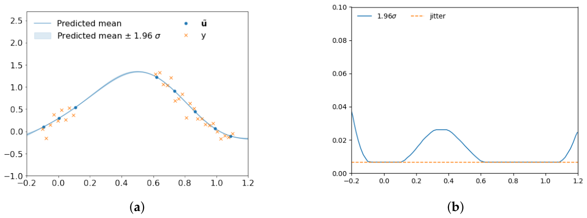
For instance, the frequently used Radial-Basis-Function (RBF) covariance function, also known as the squared-exponential covariance function, induces nonlinear functions with infinite differentiability. This results in exceptionally smooth functions, leading to highly correlated latent values. The residual variance in the latent function p f * | u ˜ is depicted in Figure 2 following the acquisition of a sample from the pseudo-point posterior, where u ˜ is drawn from q ( u ) , and predictions are made conditioned on the realisations.
The residual uncertainty in the latent function is minimal, suggesting that, given u ˜ , only a limited range of distinct realisations for the latent functions persists.

4.2. Thresholded Simulation Algorithm

The variance of the predictive distribution given the realisation up to the timestep i completely specifies the level of uncertainty for the timestep considered.
We propose a straightforward algorithm incorporating a threshold parameter T V . It is common to add jitter to all diagonal matrices in the algorithm implementation for numerical stability, and so it is added to the covariance matrix to ensure GP-model training stability. The value of jitter is supposed to be selected in a way that its influence on prediction accuracy is not significant. Consequently, delving into uncertainties smaller than the jitter is deemed impractical, introducing potential numerical complications without substantial practical utility.
The threshold parameter T V shall be selected as the value of jitter added to diagonal matrices in the implementations of training algorithms for numerical stability. We argue that setting T V below the jitter value is impractical because it can cause numerical problems. On the other hand, one should avoid selecting a larger value of the threshold parameter T V than the jitter value to retain prediction accuracy. In this way, the threshold for T V is selected unambiguously.
In this algorithm, the latent realisations are deemed informative and retained if the predictive variance at the specified timestep surpasses the designated threshold. Conversely, the corresponding latent realisations are discarded if the predictive variance falls below the threshold.
A draw from the thresholded simulation is generated using the following procedure: Initially, a sample is drawn from the posterior distribution over the pseudo-points, and this sample is subsequently added to the set of observed latent values F , i.e.,
draw u ˜ q ( u ) F = { u ˜ } .
Next, a posterior latent realisation is drawn at the timestep t + 1 , i.e.,
draw f ˜ t + 2 n a : t + 1 p ( f t + 2 n a : t + 1 | F ) , F = { u ˜ , f ˜ t + 2 n a : t + 1 } .
At timestep t + 2 , the latent realisation is drawn conditioned on preceding realisations, i.e.,
draw z ˜ t + 2 p ( z t + 2 | f ˜ t + 2 n a : t + 1 ) , draw f ˜ t + 2 p ( f t + 2 | F , z ˜ t + 2 ) , F = F , if V p ( f t + 2 | F , z ˜ t + 2 ) T V { f ˜ t + 2 , F } , if V p ( f t + 2 | F , z ˜ t + 2 ) > T V ,
where the latent observations are added to the set F only if they are considered informative, i.e., the variance exceeds the user-defined threshold. Similarly, for the timestep t + 3
draw z ˜ t + 3 p ( z t + 3 | f ˜ t + 3 n a : t + 2 ) , draw f ˜ t + 3 p ( f t + 3 | F , z ˜ t + 3 ) , F = F , if V p ( f t + 3 | F , z ˜ t + 3 ) T V { f ˜ t + 3 , F } , if V p ( f t + 3 | F , z ˜ t + 3 ) > T V .
The procedure is sequentially repeated up to the timestep t + n . The latent sample at the timestep t + n is obtained by
draw z ˜ t + n p ( z t + n | f ˜ t + i n a : t + n 1 ) , draw f ˜ t + n p ( f t + n | F , z ˜ t + n )
where F denotes the set of retained latent values. An MC approximation of the posterior latent distribution that can be seen as a GMM at an arbitrary timestep t + i is defined by
p ( f t + i | y 1 : t ) 1 r k = 1 r p ( f t + i | F k , z ˜ t + i k ) ,
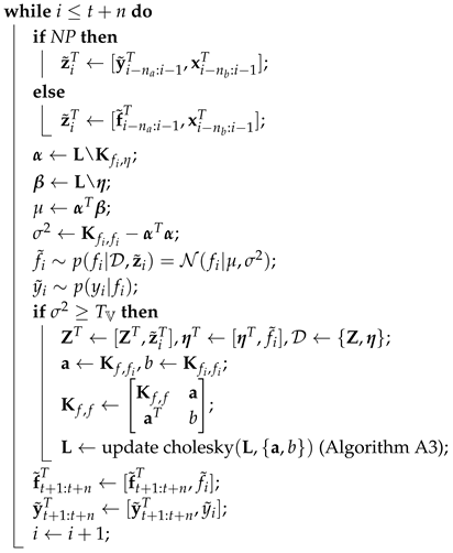
where k denotes a single sequential draw, r denotes the number of samples, and  F ( k ) represents the retained latent samples. We will refer to this approximation as the TCMC simulation. The algorithm is defined in the Appendix I as Algorithm A1.
A particular instance of TCMC simulation emerges when the threshold T V is sufficiently large, leading to the exclusion of latent observations after drawing u ˜ q ( u ) . This condition paves the way for a specialised implementation we propose as an additional contribution. Henceforth, we shall denote this unique variant as a Pseudo Independent MC (PIMC) simulation. Appendix I details the algorithm defining PIMC simulation as Algorithm A2. Conditionally Independent MC simulation (PIMC or CIMC) assumes that the latent function values up to the horizon are conditionally independent given the inputs and the noisy observations, which is not always true. The approximation is reduced if the simulation is based on TCMC, which can, in the limit, recover the ground truth.
The FCMC simulation can also be regarded as a distinctive case within the TCMC simulation framework, characterised by a threshold T V = 0 , where all latent observations are retained. Nevertheless, FCMC simulation is quite computationally complex (Table 1), while with the threshold T V 0 , the TCMC algorithm reduces the computational complexity. This can be seen in Appendix A and Appendix B’s static and dynamic system simulation results.
This simulation representation allows us to balance computational complexity against the level of approximation in the simulation. The computational complexities and memory requirements for the unified simulation of GP-NARX models are detailed in Table 1. Notably, the complexity and memory requirements of the TCMC simulation are dependent on the parameter p, representing the count of retained latent observations.
Various factors influence the practical determination of the count of retained latent observations:
  • The threshold parameter T V .
  • The selection of the covariance function.
  • Problem-specific considerations, such as learned hyperparameters.
In the upcoming section, we will conduct empirical tests to assess the performance of the simulation approximations.

5. Experimental Evaluation

This section will provide an empirical evaluation of the approximated simulation algorithms on two synthetic examples and a realistic case study, focusing on two distinct cases:
  • Sequential sampling of a static function;
  • Simulation of a GP-NARX model.
Initially, we will analyse latent distributions, comparing the FCMC estimation of the static posterior against various approximations. Subsequently, we will explore running times, the impact of various covariance functions, different sparse approximations, and the number of pseudo-inducing points. The method was also tested on several other cases for approximation error, convergence, and numerical stability, but only two cases are presented in this paper.
The practical implementation of the TCMC algorithm introduces a key distinction from the previously described approach. In the practical TCMC algorithm, latent samples are retained if, for any of the r independent MC samples, the variance of the latent posterior at the considered timestep surpasses the threshold T V . Consequently, this pragmatic strategy retains more latent observations than an individual MC run. Including a few latent observations that might otherwise be discarded ensures the preservation of the dimensionality of retained latent observations and Cholesky factors across all independent MC samples. This approach enables efficient vectorisation of the algorithm, leading to a substantial reduction in running times.
The algorithms were implemented in contemporary software frameworks, namely, TensorFlow [44] and its GP-specific extension, GPflow [45]. The following system specifications were used for experiments conducted in this section:
  • CPU: Intel(R) Core(TM) i7-8700K CPU 3.70 GHz;
  • GPU: Quadro P4000 8 GB GDDR5 [GP104GL];
  • RAM: 2 × 16 GB DIMM DDR4 3200 MHz;
  • OS: Ubuntu 18.04.5 LTS;
  • Software: GPflow 2.4.0, Tensorflow 2.4.0.
To compare the sequential estimation of the static posterior or the simulation of a GP-NARX model, we will consider a 2-Wasserstein distance W 2 [46] defined by
W 2 ( μ , ν ) 2 = | | m 1 m 2 | | 2 + Tr K 1 + K 2 2 K 2 1 2 K 1 K 2 1 2 1 2 ,
where μ N μ | m 1 , K 1 , ν N ν | m 2 , K 2 , and  K = K 1 2 K 1 2 .
In a static problem, the ground truth can be computed in closed form. However, in both static estimation with approximation and the simulation of GP-NARX models, all distributions are estimated from r independent MC samples.

5.1. Sequential Sampling of a Static Function

Firstly, we will consider sequential sampling on a static problem defined by
y = sin 3 x + 0.2 cos 10 x + N ϵ | 0 , 0 . 15 2 I .
The algorithmic structure of sequential sampling in a static model closely resembles the simulation process for GP-NARX models. However, in the static model, the latent distribution is Gaussian and can be analytically evaluated, providing an analytical solution that serves as the ground truth for comparison.
To model the problem defined by Equation (33), we employed both a VFE approximation and a FITC approximation with 30 pseudo-inputs. The latent distribution was estimated using r = 500 MC samples. Model training involved maximising the MLL through the LBFGS optimiser. In thresholded MC sampling, a threshold value of T V = 10 6 was chosen.

Discussion

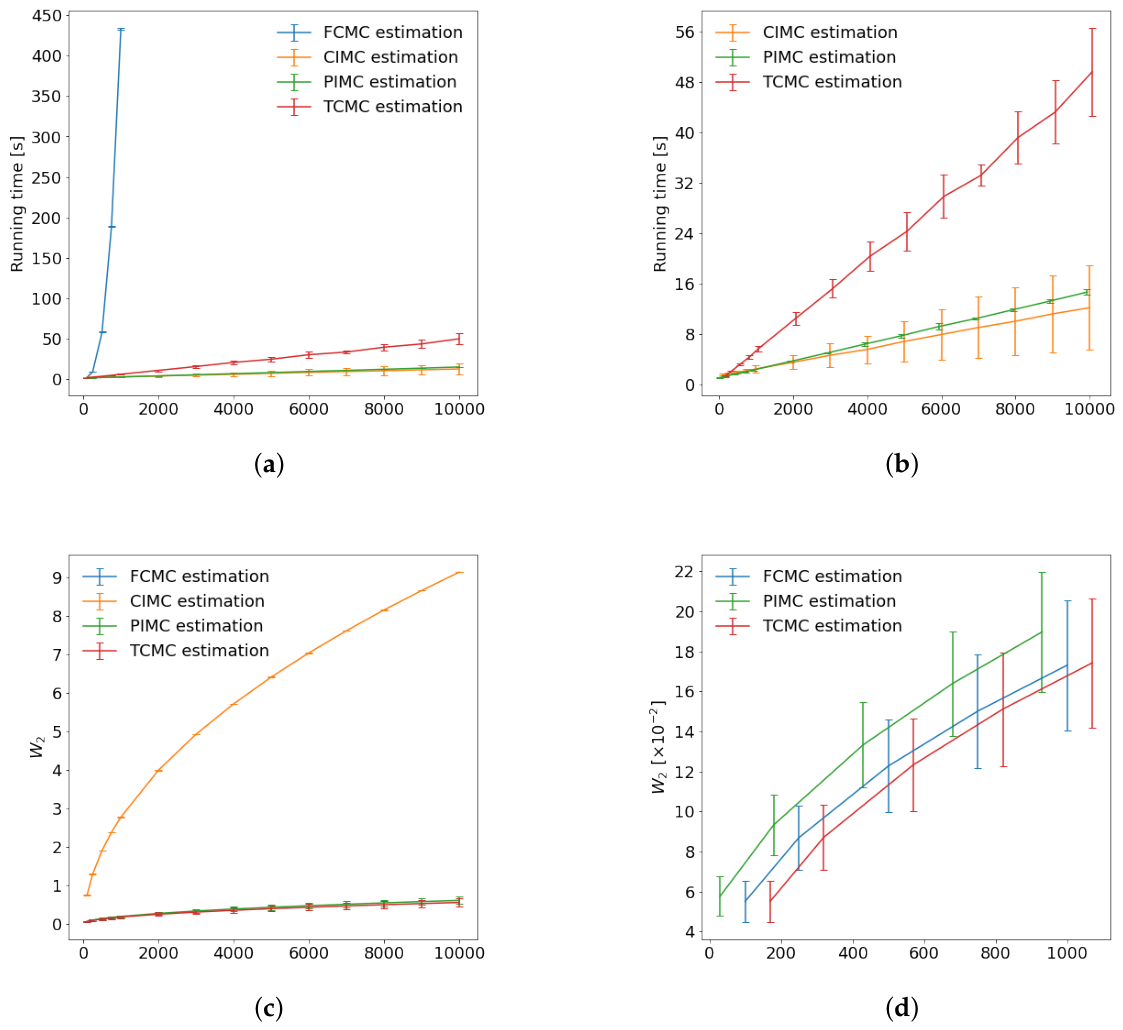
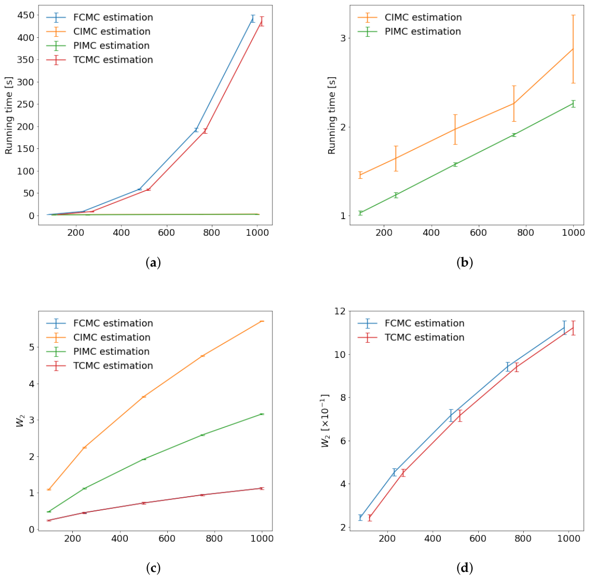
In Figure 3, the 2-Wasserstein distance is illustrated between the closed-form solution of the latent distribution and the estimated distribution from samples for the Matérn( 5 2 ) covariance function [6]. Results for the other covariance functions in the Matérn family can be found in Appendix A and the definitions in Appendix C. The figures additionally present the running times of various numerical approximations for sequential sampling, demonstrating their performance with respect to an increasing number of input locations.
The computational demands of FCMC static posterior estimation exhibit cubic computational complexity, rendering them impractical for large numbers of test inputs. Conversely, TCMC estimation proves computationally feasible and is accomplished in a significantly shorter timeframe than FCMC. For instance, when considering the Matérn( 5 2 ) covariance function, the running time of TCMC is only 10% of that required for FCMC estimation when processing 600 test inputs. Nevertheless, the effectiveness of TCMC depends on the smoothness of the covariance function. The selection of a suitable covariance function is an important part of efficient model design, and it also affects the efficiency of model simulation.
Upon closer examination of the 2-Wasserstein distance, computed up to the 600 test inputs for the FCMC, it becomes apparent that the TCMC estimation error closely mirrors that of the FCMC estimation. This similarity arises from the adoption of a very low threshold value, i.e.,  T V = 10 6 . By setting the threshold as low as the numerical jitter, the TCMC estimation recovers the FCMC results, achieving this outcome at only a fraction of the running time for covariance functions that generate relatively smooth functions.
While even less computationally demanding, PIMC and CIMC estimations introduce a discernible error, as indicated by the 2-Wasserstein distance in the earlier figures. This discrepancy is particularly noticeable in CIMC estimation, where the 2-Wasserstein distance is relatively high compared to FCMC estimation.
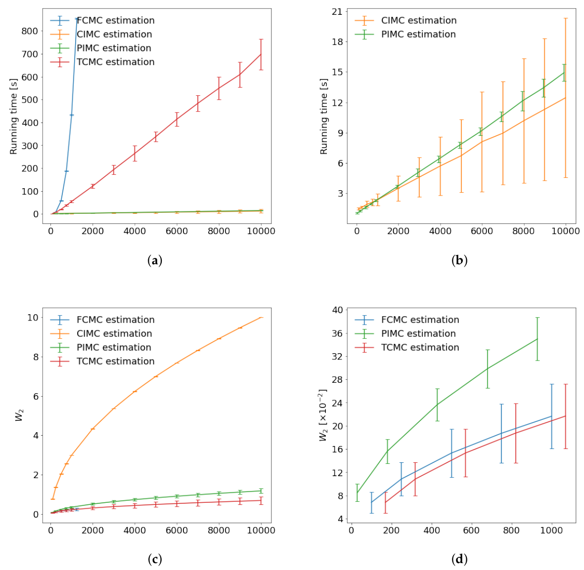
If the functions induced by the covariance functions exhibit greater roughness, as seen with the Matérn( 3 2 ) and Matérn( 1 2 ) covariance functions in Appendix A, the computational advantages of the thresholded sampler diminish. For the Matérn( 1 2 ) covariance function, these benefits are eliminated. Therefore, the effectiveness of TCMC depends on the smoothness of the covariance function. The selection of a suitable covariance function is an important part of efficient model design, and it also affects the efficiency of model simulation. In situations involving the Matérn( 1 2 ) covariance function, defaulting to CIMC and PIMC estimation is often necessary. However, a considerable error is expected, as demonstrated by the 2-Wasserstein distance.
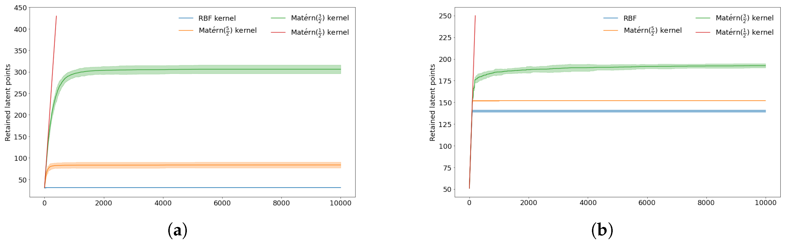
In Figure 4, the plot illustrates the retained latent points concerning the increasing number of test locations for various covariance functions and GP approximations. It is evident that, at a certain point, the number of retained points reaches saturation, and keeping more latent values does not provide benefits. Compared to rougher kernel functions, the saturation point arrives earlier for smoother covariance functions.
For instance, in the case of the Matérn( 1 2 ) covariance function, characterised by highly uncorrelated data points between neighbouring inputs, nearly all latent points are retained. The curve for Matérn( 1 2 ) can be regarded as a representative proxy for the retained latent points in scenarios involving FCMC estimation. The retained latent points derived from the FCMC estimation of the Matérn( 3 2 ) covariance function would, for example, closely align with the curve from the TCMC estimation of the Matérn( 1 2 ) covariance function.
While the sequential estimation in static problems shares similarities with the simulation of GP-NARX models, it is important to note that the issues are distinct. Nevertheless, having a closed-form solution for comparison purposes is advantageous. In static problems, consecutive latent samples have no input/output dependency between consecutive latent samples. As a result, a single Cholesky factor can be computed for multiple independent MC samples, leading to a substantial reduction in running times and memory requirements for the algorithms. In the subsequent section, we will explore these approximations within the context of an illustrative dynamical system.

5.2. Simulation of a Dynamical System

We consider an illustrative problem [37], where the difference equation governs the true process
f t + 1 1 = f t 1 exp 1 0.4 f t 1 2 + 1.2 x t 1 f t 2 1 + f t 1 2 , f t + 1 2 = f t 2 exp 1 0.5 x t 1 1.5 x t 2 f t 2 f t 1 , x t 1 = cos 2 π t , x t 2 = sin 2 π t .
We observe noisy values
y t 1 N y t 1 | f t 1 , σ n 2 , y t 2 N y t 2 | f t 2 , σ n 2 .
For the training data, the system was initialised with [ f 0 1 , f 0 2 ] = [ 0.300 , 0.800 ] and simulated for 900 samples. The test data utilised an initialisation of [ f 0 1 , f 0 2 ] = [ 0.380 , 0.326 ] , and the simulation was conducted for the specified number of samples. Gaussian noise with σ n 2 = 10 2 was introduced to corrupt the data. NARX model parameters were set as n a = n b = 4 . The system was modelled by a GP-NARX (VFE) model with 50 pseudo-inputs. The latent distribution was estimated using r = 500 MC samples. Hyperparameters were determined through MLL maximisation with the LBFGS optimiser. In the TCMC simulation, a threshold of T V = 10 6 was selected.

Discussion

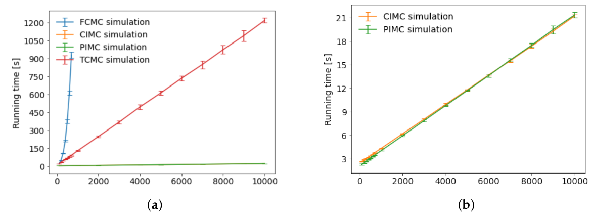
In Figure 5, the running times of the simulation are illustrated up to 10,000 steps into the future for the Matérn( 5 2 ) covariance function. The results for the other covariance functions in the Matérn family are shown in Appendix A. The running times for the FCMC simulation escalate rapidly, mirroring the trend observed in the static case. As the prediction horizon extends, the FCMC simulation cannot be practically realised.
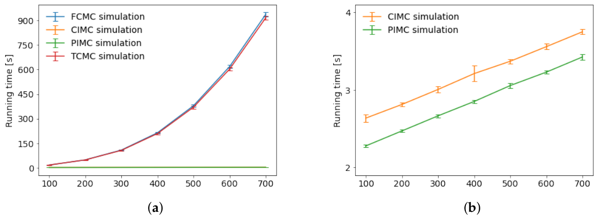
The approximations are computed within a reasonable time frame, as demonstrated for the Matérn( 5 2 ) and Matérn( 3 2 ) covariance functions, i.e., covariance functions that generate relatively smooth functions. Nevertheless, it is noteworthy that running times in simulation are considerably higher compared to static estimation, as a distinct Cholesky factor needs to be computed for each independent MC sample.
For the Matérn( 1 2 ) covariance function, the running times of the TCMC simulation do not exhibit a reduction when compared to the FCMC simulation. In this scenario, the TCMC simulation is not practically feasible for large prediction horizons since nearly all latent samples are retained, resulting in a simulation closely resembling the FCMC counterpart. One alternative is to employ an approximation with additional assumptions, such as the PIMC and CIMC simulations. However, as the 2-Wasserstein distance demonstrates, it is essential to anticipate some error in estimating the latent response.
However, the commonly employed CIMC approximation in the literature shows no discernible advantages compared to the proposed PIMC simulation. The response estimated through a PIMC simulation offers a superior approximation to the FCMC and can be obtained within the same computational time as the CIMC simulation. Consequently, in situations where the TCMC simulation cannot be obtained, opting for the PIMC simulation is recommended over the CIMC simulation.
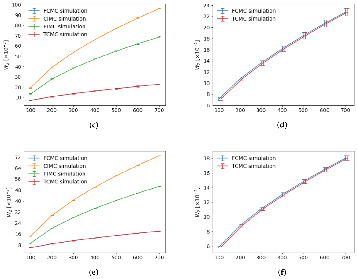
For smoother covariance functions, such as Matérn( 5 2 ) and Matérn( 3 2 ) covariance functions, the TCMC simulation significantly reduces the running time of the simulation while maintaining a 2-Wasserstein distance practically identical to that in the FCMC simulation. The chosen threshold T V = 10 6 in this section is equivalent to the jitter added to covariance matrices for numerical stability, representing the level of variance we are willing to sacrifice for improved numerical conditioning. When the threshold matches the numerical jitter, the TCMC simulation can be considered essentially equivalent to the FCMC simulation. This ensures a reasonable computation time and scalability to larger predictive horizons.
Figure 4 illustrates the retained latent points concerning the increasing number of predicted steps into the future for different covariance functions. Once more, it is apparent that, at a certain point, the number of retained points reaches saturation. Again, we can observe that the Matérn( 1 2 ) covariance function serves as a proxy for the FCMC simulation.
The synthetic examples show that the TCMC simulation efficiently recovers the FCMC results within significantly less computational time when dealing with relatively smooth functions. However, the computational advantages diminish for covariance functions that induce rougher functions. This, however, is generally not problematic in practice for the following reasons:
  • Smooth functions are often preferred for small data sets as they tend to generalise better;
  • The choice of the covariance function becomes less critical for larger data sets;
  • In the case of large data sets, the uncertainty of the latent function posterior is typically relatively small.
The first point emphasises the preference for well-regularised models, often achieved through some smoothness assumption. In the context of GP-specific models, this assumption is defined on a meta-level, reflecting the properties of functions induced by respective covariance functions. An example of such a smoothness assumption is the level of differentiability, indicating how many times the function is differentiable.
The second point pertains to selecting the covariance function, particularly in the context of large data sets. In such cases, the abundance of data is a penalty for overly flexible models, rendering the choice of the covariance function less critical. Models employing various covariance functions, yet appropriately flexible to mitigate bias, are anticipated to exhibit relatively similar performance. This consideration becomes relevant when the objective is to simulate data over extended prediction horizons in the simulation of GP-NARX models. A preference for a smoother covariance function may be justified, especially if the model’s performance does not change substantially.
The third point emphasises that the uncertainty associated with the expected latent function posterior tends to be relatively small in large data sets. This latent uncertainty captures the epistemic uncertainty arising from the lack of observed data. As more data become available, the latent uncertainty diminishes, requiring fewer latent samples to adequately characterise the latent function.
The upcoming section will showcase the simulation approximations using a real-world example.

5.3. Case Study

In the previous examples, our focus was not on model selection, such as determining the optimal covariance function, but rather on benchmarking the performance of simulation algorithms. In this section, we will delve into modelling a more complex dynamical benchmark. This benchmark entails a relatively large training data set, making it impractical to employ the vanilla GP-NARX model in practice [38]. Despite sparse models approximating the training process, the test data sets are too extensive for the FCMC simulation to be feasible. Our aim here is to showcase the application of the TCMC simulation on this benchmark.
Silverbox benchmark represents the second-order linear time-invariant system with the third-degree polynomial static nonlinearity around it in feedback. It is a real-world system that collects data from an electric circuit [47]. The system theoretically obeys the equation
m d 2 y ( t ) d t 2 d d y ( t ) d t + a y ( t ) + b y ( t ) 3 = u ( t ) .
We selected the training data from samples 40,586 to 127,410 and the test data as the first 40,495 samples [48]. The system was excited with a white Gaussian noise sequence filtered by a ninth-order discrete-time Butterworth filter. Training data were obtained by exciting ten successive realisations of a random odd multi-sine signal [47]. We additionally standardised the data and added Gaussian noise to the observations with the standard deviation of σ n = 5 × 10 2 .
The meta-parameters of the NARX model were selected as n b = n a = 5 . We used 300 pseudo-inputs initialised with the k-means clustering algorithm as suggested in [11]. The hyperparameters and the pseudo-input locations were determined by MLL maximisation using the Limited-Memory Broyden-Fletcher-Goldfarb-Shanno (LBFGS) optimiser [49].

Discussion

Table 2 presents the outcomes of the 10-fold cross-validation on the training data. Notably, for the Silverbox dataset, the most effective combination involves a linear and a Matérn( 5 2 ) covariance function, closely followed by a combination of a linear and a Matérn( 3 2 ) covariance function. The performance metrics indicate that the model describes the data well in terms of both mean values, as evident in the RMSE and standardised mean squared error (SMSE) metrics [5], and probability distributions, as indicated by the mean standardised log loss (MSLL) metric [5].
Table 3 presents the outcomes of prediction and simulation on the test data using the top two covariance functions selected through cross-validation. Analogous to the prediction results, the performance metrics affirm that the model adeptly describes the data, extending its capability to simulation. The simulation results exhibit negligible variations among the employed approximations, as seen with the performance metrics.
Notably, the TCMC simulation, which practically recovers the FCMC results, in our case considered as ground truth, is attainable on a personal computer. However, its running time remains impractical for scenarios where the simulation needs to be repeated multiple times (as in cross-validation or rolling forecasts) or when more real-time forecasts are required.
In contrast, the PIMC simulation, previously observed to outperform the CIMC approximation, can be obtained in just 5% of the time required for the TCMC simulation. Hence, the PIMC simulation emerges as a convenient alternative, effectively balancing computational complexity with the accuracy of the estimated latent response.

6. Conclusions

GP models offer a probabilistic regression approach characterised by the elegance of the nonparametric function estimation. They reduce the need for strict assumptions or at least elevate them to a higher level. This mechanism presents a more systematic regression approach compared to other contemporary forecasting methods, where the selection of meta-parameters often involves an element of uncertainty.
Various approximations have partially alleviated the computational burden of GP models, marked by cubic complexity regarding the training data. A common strategy involves learning a set of pseudo-points to capture a sparse representation of the underlying data. Nevertheless, this approach primarily benefits static systems, where MLL and predictions can be obtained analytically.
Given the inherent propagation of uncertain inputs during training and multi-step-ahead predictions, the challenge intensifies when dealing with dynamical systems. In the training phase, autoregression can simplify the dynamical problem to that of the static case. However, simulating such autoregressive models remains a significant challenge due to the absence of analytical solutions, often necessitating MC estimation. This, in turn, imposes substantial computational demands and mandates specific algorithms tailored to each sparse approximation.
In this investigation, we proposed a unified simulation framework invariant to sparse and variations approximations up to obtaining a static sample from the pseudo-point posterior. This framework incorporates all known numerical simulations of GP-NARX models.
Moreover, we introduced a novel MC estimation algorithm for simulating autoregressive GP models. This algorithm addresses the computational complexity and specificity challenges associated with conventional MC algorithms tailored for individual sparse approximations. The presented algorithm is a versatile plug-and-play solution applicable across various sparse approximations.
When acquiring an utterly accurate simulation is infeasible, our proposed algorithm, Thresholded Conditional MC (TCMC), provides a close approximation to what can be regarded as the ground truth, i.e., FCMC, up to numerical precision. A specialised TCMC variant, PIMC simulation, can be employed for scenarios with stricter time constraints. PIMC attains simulation speeds comparable to static counterparts while outperforming existing CIMC approximations in accuracy.
The PIMC simulation does not keep the consecutive latent observations in memory. However, some latent uncertainty is still reduced, especially in kernels that induce smooth functions. PIMC should be preferred over the CIMC simulation since it better approximates the ground truth and has the same computational complexity.
TCMC simulation can reduce computational requirements and improve estimation of the latent response compared with CIMC and PIMC simulations. It introduces a tradeoff parameter that can maximise the computational resources and, consequently, the quality of the estimated latent response. If the threshold equals the numerical jitter, the TCMC simulation retrieves the FCMC simulation for only a fraction of the computational cost of the ground truth when kernels that induce smooth functions are used.
To assess the efficacy of these approximations, we conducted comparisons using a static system with analytically obtainable ground truth and an illustrative dynamical example. Furthermore, we validated the algorithmic performance by applying it to model a real-world case study with a substantial dataset. Notably, the simulations were successfully executed on a personal computer, a task previously deemed unattainable.
Following the proof of concept presented in this publication, more practical applications of the method are envisaged. Potential examples of uncertainty propagation in GP-ARX models include continuous-time Simultaneous Localisation and Mapping (SLAM) [50] and Gaussian Process Occupancy Mapping (GP-OM) for 3D point clouds [51] in the field of robotics. In SLAM, the propagation of robot odometry uncertainty over time is inherently an autoregressive process, and modelling the continuous probability distribution of dense point clouds with GPs is computationally expensive due to the large number of data points. The core philosophy of the TCMC algorithm—dynamically discarding latent variables when the predictive variance falls below the threshold T V —is mathematically analogous to dynamically downsampling redundant Lidar point clouds in map regions where the surface probability is already highly confident.
Moreover, for future endeavours in advancing the simulation of the GP-NARX model, a focus on refining the trade-off between computational complexity and the precision of the estimated response is warranted. In addition, special attention will be given to assessing uncertainty calibration, long-horizon stability, or preservation of temporal dependence structures when using FCMC. An intriguing avenue for future exploration is a hybrid approach that combines the efficiency of the TCMC simulation with samplers designed to approximate the latent posterior using basis functions at test time. This integrated strategy is expected to enhance computational efficiency and response accuracy, offering a promising direction for further research.

Author Contributions

Conceptualisation, T.K. and J.K.; methodology, T.K.; software, T.K.; validation, T.K. and J.K.; investigation, T.K.; resources, T.K.; data curation, T.K.; writing—original draft preparation, T.K.; writing—review and editing, T.K. and J.K.; project administration, J.K.; funding acquisition, J.K. All authors have read and agreed to the published version of the manuscript.

Funding

The authors acknowledge that the Slovenian Research and Innovation Agency financially supported research core funding No. P2-0001 and a PhD grant for Tadej Krivec.

Data Availability Statement

The data presented in this study are openly available in GitHub at https://github.com/tadejkrivec/GPflow-NARX (accessed on 10 June 2026).

Conflicts of Interest

The authors declare no conflicts of interest.

Appendix A. Sequential Sampling of a Static Function

Figure A1. The 2-Wasserstein distance and the running times for the VFE approximation in the sequential estimation of the latent distribution using the Matérn( 3 2 ) covariance function. (a) Running times for the VFE approximation and the Matérn( 3 2 ) covariance function. (b) Closer view of running times for the VFE approximation and the Matérn( 3 2 ) covariance function. (c) 2-Wasserstein distance for the VFE approximation and the Matérn( 3 2 ) covariance function. (d) Closer view of the 2-Wasserstein distance for the VFE approximation and the Matérn( 3 2 ) covariance function.
Mathematics 14 02111 g0a1
Figure A2. The 2-Wasserstein distance and the running times for the VFE approximation in the sequential estimation of the latent distribution using the Matérn( 1 2 ) covariance function. (a) Running times for the VFE approximation and the Matérn( 1 2 ) covariance function. (b) Closer view of running times for the VFE approximation and the Matérn( 1 2 ) covariance function. (c) 2-Wasserstein distance for the VFE approximation and the Matérn( 1 2 ) covariance function. (d) Closer view of the 2-Wasserstein distance for the VFE approximation and the Matérn( 1 2 ) covariance function.
Mathematics 14 02111 g0a2

Appendix B. Simulation of a Dynamical System

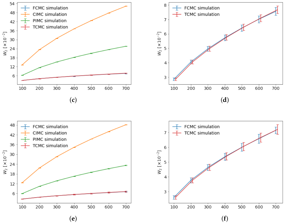
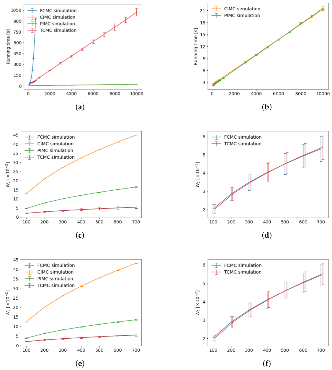
Figure A3. The 2-Wasserstein distance and the running times for the simulation of the GP-NARX (VFE) model using the Matérn( 3 2 ) covariance function. (a) Running time comparison of the simulation. (b) Closer view of the running time comparison of the simulation. (c) 2-Wasserstein distance for f 1 . (d) Closer view of the 2-Wasserstein distance for f 1 . (e) 2-Wasserstein distance for f 2 . (f) Closer view of the 2-Wasserstein distance for f 2 .
Mathematics 14 02111 g0a3aMathematics 14 02111 g0a3b
Figure A4. The 2-Wasserstein distance and the running times for the simulation of the GP-NARX (VFE) model using the Matérn( 1 2 ) covariance function. (a) Running time comparison of the simulation. (b) Closer view of the running time comparison of the simulation. (c) 2-Wasserstein distance for f 1 . (d) Closer view of the 2-Wasserstein distance for f 1 . (e) 2-Wasserstein distance for f 2 . (f) Closer view of the 2-Wasserstein distance for f 2 .
Mathematics 14 02111 g0a4aMathematics 14 02111 g0a4b

Appendix C. Covariance Functions

Matérn Covariance Functions

The definitions of the Matérn covariance functions are the following:
k Matérn ( ν = 1 2 ) ( x i , x j ) = σ f 2 e r ,
k Matérn ( ν = 3 2 ) ( x i , x j ) = σ f 2 ( 1 + 3 r ) e 3 r ,
k Matérn ( ν = 5 2 ) ( x i , x j ) = σ f 2 ( 1 + 5 r + 5 3 r 2 ) e 5 r ,
k Matérn ( ν = ) ( x i , x j ) = k RBF ( x i , x j ) = σ f 2 e r 2 2 ,
where r = 1 l | | x i x j | | . Kernels with the automatic relevance determination (ARD) property define
r = ( x i x j ) T Λ 1 ( x i x j ) ,
where Λ 1 = diag ( [ l 1 2 , , l d 2 ] ) and d is the number of columns in x .

Appendix D. Model Learning

This appendix provides a quick overview of training sparse Gaussian process models.
When the datasets are relatively large, a popular approach is to maximise the logarithm of the marginal likelihood or the ELBO with respect to the hyperparameters, i.e.,
Θ ^ = arg max Θ log F Θ ,
where Θ represents the free parameters of F. Explicit definitions of F Θ for various approximations can be found in Appendix D. The evaluation of F Θ of a vanilla GP-NARX model results in a computational complexity of O ( t 3 ) , where t denotes the number of observed time steps. The training of the GP-NARX (FITC) and GP-NARX (VFE) results in a computational complexity of O ( t m 2 ) , where m denotes the number of pseudo-inputs. The training of the GP-NARX (SVGP) models results in a computational complexity O ( m 3 ) . The memory requirements for the vanilla GP-NARX model are O ( t 2 ) and O ( m 2 ) for sparse approximations. The following sections provide unified descriptions of the GP-NARX model’s prediction and simulation.

Appendix E. Marginal Likelihoods

Appendix E.1. GP-NARX (Vanilla)

F Θ = F θ , σ n 2 = 1 2 y 1 : t T K f 1 : t , f 1 : t + I σ n 2 1 y 1 : t 1 2 log K f 1 : t , f 1 : t + I σ n 2 n 2 log 2 π

Appendix E.2. GP-NARX (FITC)

F Θ = F θ , σ n 2 , z 1 : m = 1 2 y 1 : t T Q f 1 : t , f 1 : t diag Q f 1 : t , f 1 : t K f 1 : t , f 1 : t + I σ n 2 1 y 1 : t 1 2 log Q f 1 : t , f 1 : t diag Q f 1 : t , f 1 : t K f 1 : t , f 1 : t + I σ n 2 n 2 log 2 π

Appendix E.3. GP-NARX (VFE)

F Θ = F θ , σ n 2 , z 1 : m = log [ N ( y 1 : t | 0 , Q f 1 : t , f 1 : t + I σ n 2 ) ] 1 2 σ n 2 tr ( K f 1 : t , f 1 : t Q f 1 : t , f 1 : t )

Appendix E.4. GP-NARX (SVGP)

F Θ = F θ , σ n 2 , z 1 : m , m , Φ = n = 1 t E q ( f n ) log p ( y n | f n ) KL q ( u ) | | p ( u ) ,
where
p ( y n | f n ) = N y n | f n , σ n 2 , q ( u ) = N u | m , Φ , p ( u ) = N u | 0 , K u , u ,
and KL defines the Kullback–Leibler divergence between q ( u ) and p ( u ) .

Appendix F. Predictive Posteriors

This section defines the predictions in GP-NARX models, i.e.,  p ( f t + 1 | y 1 : t ) = N E [ f t + 1 | y 1 : t ] , V [ f t + 1 | y 1 : t ] .

Appendix F.1. GP-NARX

The mean of the predictive posterior is defined by
E [ f t + 1 | y 1 : t ] = K f t + 1 , f 1 : t K f 1 : t , f 1 : t + I σ n 2 1 y 1 : t .
The variance of the predictive posterior is defined by
V [ f t + 1 | y 1 : t ] = K f t + 1 , f t + 1 K f t + 1 , f 1 : t K f 1 : t , f 1 : t + I σ n 2 1 K f 1 : t , f t + 1 .

Appendix F.2. GP-NARX (FITC)

The mean of the predictive posterior is defined by
E [ f t + 1 | y 1 : t ] = K f t + 1 , u K u , u + K u , f 1 : t Λ 1 K f 1 : t , u 1 K u , f 1 : t Λ 1 y 1 : t ,
where
Λ = diag K f 1 : t , f 1 : t K f 1 : t , u K u , u 1 K u , f 1 : t + I σ n 2 .
The variance of the predictive posterior is defined by
V [ f t + 1 | y 1 : t ] = K f t + 1 , f t + 1 K f t + 1 , u K u , u 1 K u , f t + 1 .

Appendix F.3. GP-NARX (VFE)

The mean of the predictive posterior is defined by
E [ f t + 1 ] = σ n 2 K f t + 1 , u K u , u + σ n 2 K u , f 1 : t K f 1 : t , u 1 K u , f 1 : t y 1 : t .
The variance of the predictive posterior is defined by
V [ f t + 1 ] = K f t + 1 , f t + 1 K f t + 1 , u K u , u 1 K u , f t + 1 + K f t + 1 , u K u , u + σ n 2 K u , f 1 : t K f 1 : t , u 1 K u , f t + 1 .

Appendix F.4. GP-NARX (SVGP)

The mean of the predictive posterior is defined by
E [ f t + 1 ] = K f t + 1 , u K u , u 1 m .
The variance of the predictive posterior is then defined by
V [ f t + 1 ] = K f t + 1 , f t + 1 K f t + 1 , u K u , u 1 K u , f t + 1 + K f t + 1 , u K u , u 1 Φ K u , u 1 K u , f t + 1 ,
where q ( u ) = N u | m , Φ .

Appendix G. Pseudo-Point Posteriors

Appendix G.1. GP-NARX (Vanilla)

In GP-NARX (Vanilla), the pseudo-point posterior is defined by q ( u ) = p ( f 1 : t | y 1 : t ) , where the mean and the variance of the respective Gaussian distribution are defined by
E [ f 1 : t | y 1 : t ] = K f 1 : t , f 1 : t K f 1 : t , f 1 : t + I σ n 2 1 y 1 : t ,
V [ f 1 : t | y 1 : t ] = K f 1 : t , f 1 : t K f 1 : t , f 1 : t K f 1 : t , f 1 : t + I σ n 2 1 K f 1 : t , f 1 : t .

Appendix G.2. GP-NARX (FITC)

In GP-NARX (FITC), the pseudo-point posterior is defined by q ( u ) = p ( u | y 1 : t ) , where the mean and the variance of the respective Gaussian distribution are defined by
E [ u | y 1 : t ] = K u , u K u , u + K u , f 1 : t Λ 1 K f 1 : t , u 1 K u , f 1 : t Λ 1 y 1 : t ,
V [ u | y 1 : t ] = K u , u K u , u + K u , f 1 : t Λ 1 K f 1 : t , u 1 K u , u ,
where
Λ = diag K f 1 : t , f 1 : t K f 1 : t , u K u , u 1 K u , f 1 : t + I σ n 2 .

Appendix G.3. GP-NARX (VFE)

In GP-NARX (VFE), the pseudo-point posterior is defined by q ( u ) p ( u | y 1 : t ) , where the mean and the variance of the respective Gaussian distribution are defined by
E [ u ] = σ n 2 K u , u K u , u + σ n 2 K u , f 1 : t K f 1 : t , u 1 K u , f 1 : t y 1 : t ,
V [ u ] = K u , u K u , u + σ n 2 K u , f 1 : t K f 1 : t , u 1 K u , u .

Appendix G.4. GP-NARX (SVGP)

In GP-NARX (SVGP), the pseudo-point posterior is defined by q ( u ) p ( u | y 1 : t ) , where the mean and the variance of the respective Gaussian distribution are directly parametrised by the free variational parameters, i.e.,   
E [ u ] = m ,
V [ u ] = Φ .

Appendix H. Simulation Approximations

This section presents the simulation approaches used throughout this study and summarises their underlying posterior assumptions. In summary, Fully Correlated Monte Carlo simulation conditions on all latent values. Pseudo Independent Monte Carlo simulation conditions on posterior pseudo-point realisations, rendering the simulated values conditionally independent given these realisations. Conditionally Independent Monte Carlo simulation further marginalises over the posterior pseudo-point realisations and assumes conditional independence among the simulated latent values. Naive simulations provide a non-Monte Carlo alternative by propagating only the posterior means. Finally, thresholded correlated simulation conditions are applied to a subset of latent values, where retention is determined by the uncertainty associated with each posterior prediction.

Appendix H.1. Fully Correlated Monte Carlo Simulation

q f t + 1 : t + n   = p ( f t + 2 n a : t + 1 | u ) q u   · i = 2 n p ( f t + i | f t + 1 : t + i 1 , u , z t + i ) p ( z t + i | f t + i n a : t + i 1 ) d z t + i d f { f t + 1 : t + n } d u .

Appendix H.2. Pseudo Independent Monte Carlo Simulation

q f t + 1 : t + n   = p ( f t + 2 n a : t + 1 | u ) q u   · i = 2 n p ( f t + i | f t + 1 : t + i 1 , u , z t + i ) p ( z t + i | f t + i n a : t + i 1 ) d z t + i d f { f t + 1 : t + n } d u   = p ( f t + 2 n a : t + 1 | u ) q u   · i = 2 n p ( f t + i | u , z t + i ) p ( z t + i | f t + i n a : t + i 1 ) d z t + i d f { f t + 1 : t + n } d u .

Appendix H.3. Conditionally Independent Monte Carlo Simulation

q f t + 1 : t + n   = p ( f t + 2 n a : t + 1 | u ) q u   · i = 2 n p ( f t + i | f t + 1 : t + i 1 , u , z t + i ) p ( z t + i | f t + i n a : t + i 1 ) d z t + i d f { f t + 1 : t + n } d u   = p ( f t + 2 n a : t + 1 | u ) q u   · i = 2 n p ( f t + i | u , z t + i ) p ( z t + i | f t + i n a : t + i 1 ) d z t + i d f { f t + 1 : t + n } d u   = q ( f t + 2 n a : t + 1 )   · i = 2 n p ( f t + i | u , z t + i ) q ( u ) p ( z t + i | f t + i n a : t + i 1 ) d z t + i d u d f { f t + 1 : t + n }   = q ( f t + 2 n a : t + 1 ) i = 2 n q ( f t + i | z t + i ) p ( z t + i | f t + i n a : t + i 1 ) d z t + i d f { f t + 1 : t + n } .

Appendix H.4. Fully Correlated Naive Simulation

q f t + 1 : t + n =   = p ( f t + 2 n a : t + 1 | u ) q u   · i = 2 n p ( f t + i | f t + 1 : t + i 1 , u , z t + i ) p ( z t + i | μ t + i n a : t + i 1 ) d z t + i d f { f t + 1 : t + n } d u .
where
p ( z t + i T | μ t + i n a : t + i 1 ) = δ z t + i T [ μ t + i n a : t + i 1 T , x t + i n b : t + i 1 T ] , μ t + i n a : t + i 1 = E p ( f t + i n a : t + i 1 | y 1 : t ) .

Appendix H.5. Conditionally Independent Naive Simulation

q f t + 1 : t + n =   = p ( f t + 2 n a : t + 1 | u ) q u   · i = 2 n p ( f t + i | f t + 1 : t + i 1 , u , z t + i ) p ( z t + i | μ t + i n a : t + i 1 ) d z t + i d f { f t + 1 : t + n } d u   = q ( f t + 2 n a : t + 1 ) i = 2 n q ( f t + i | z t + i ) p ( z t + i | μ t + i n a : t + i 1 ) d z t + i d f { f t + 1 : t + n } ,
where p ( z t + i | μ t + i n a : t + i 1 ) is defined by Equation (A27).

Appendix H.6. Thresholded Correlated Simulation

q f t + 1 : t + n   = p ( f t + 2 n a : t + 1 | u ) q u   · i = 2 n p ( f t + i | f F , u , z t + i ) p ( z t + i | f t + i n a : t + i 1 ) d z t + i d f { f t + 1 : t + n } d u ,
where F denotes the set of retained latent function values based on the Algorithm A1.

Appendix I. Algorithms

This section presents the algorithms for the Monte Carlo simulation methods introduced in this publication. We assume that the pseudo-input locations Z 1 : m have been obtained during model training and treat them as fixed, as their estimation is not the focus of this work. The posterior distribution of the lagged latent values is available in closed form, and the initial realisations are obtained by sampling from this distribution.

Appendix I.1. Thresholded Correlated Monte Carlo Simulation

Algorithm A1: Algorithm for a single sample in the TCMC simulation of the GP-NARX models. The pseudo-point posteriors for the respective GP-NARX model are defined in Appendix G. PIMC simulation corresponds to the variance threshold T V = . FCMC simulation corresponds to the variance threshold T V = 0 . NP denotes noise propagation.
Data:  T V : variance threshold
Data:  Z 1 : m : pseudo-input locations
Data:  q ( u ) = N ( u | m , Φ ) : posterior at the pseudo-input locations Z 1 : m for the respective GP-NARX model
Result:  f ˜ t + 1 : t + n : sample of the latent trajectory
Result:  y ˜ t + 1 : t + n : sample of the noisy trajectory
f ˜ t + 1 n a : t q ( f t + 1 n a : t ) ;
f ˜ t + 1 : t + n [ c ] ;
y ˜ t + 1 : t + n [ c ] ;
i t + 1 ;
K f , f K u , u ;
L L T cholesky ( K f , f ) ;
u ˜ q ( u ) ;
Z Z 1 : m , η u ˜ , D { Z , η } ;
Mathematics 14 02111 i001

Appendix I.2. Pseudo Independent Monte Carlo Simulation

Algorithm A2: Algorithm for a single sample in the PIMC simulation of the GP-NARX models. NP denotes noise propagation.
Data:  Z 1 : m : pseudo-input locations
Data:  q ( u ) = N ( u | m , Φ ) : posterior at the pseudo-input locations Z 1 : m for the respective GP-NARX model
Result:  f ˜ t + 1 : t + n : sample of the latent trajectory
Result:  y ˜ t + 1 : t + n : sample of the noisy trajectory
f ˜ t + 2 n a : t + 1 q ( f t + 2 n a : t + 1 ) ;
y ˜ t + 1 p ( y t + 1 | f t + 1 ) ;
f ˜ t + 1 : t + n [ f ˜ t + 1 ] T ;
y ˜ t + 1 : t + n [ y ˜ t + 1 ] T ;
i t + 2 ;
u ˜ q ( u ) ;
D { Z 1 : m , u ˜ } ;
L u L u T cholesky ( K u , u ) ;
L u 1 L u \ I ;
γ L u T L u 1 ;
δ γ u ˜ ;
Mathematics 14 02111 i002

Appendix I.3. Cholesky Update

Algorithm A3: Algorithm for the iterative update of the Cholesky factor. Updates the Cholesky factor based on a row/column addition to the covariance matrix.
Data:  L R m × m : cached Cholesky factor
Data:  { a , b } : column addition to the covariance matrix, a represents the cross-covariance between the new point and the existing points, and b the covariance of the added point.
Result:  L ^ R ( m + 1 ) × ( m + 1 ) : updated Cholesky factor
α L \ a ;
β b α T α ;
L ^ L 0 α T β

References

  1. Gregorčič, G.; Lightbody, G. Gaussian process approach for modelling of nonlinear systems. Eng. Appl. Artif. Intell. 2009, 22, 522–533. [Google Scholar] [CrossRef] [Scilit]
  2. Capone, A.; Lederer, A.; Hirche, S. Gaussian process uniform error bounds with unknown hyperparameters for safety-critical applications. In Proceedings of the International Conference on Machine Learning, PMLR, Baltimore, MD, USA, 17–23 July 2022; pp. 2609–2624. [Google Scholar]
  3. Yi, Y.; Verbič, G. Operating Envelopes under Probabilistic Electricity Demand and Solar Generation Forecasts. arXiv 2022, arXiv:2207.09818. [Google Scholar] [CrossRef] [Scilit]
  4. Krige, D.G. A statistical approach to some basic mine valuation problems on the Witwatersrand. J. South. Afr. Inst. Min. Metall. 1951, 52, 119–139. [Google Scholar]
  5. Rasmussen, C.E.; Williams, C.K. Gaussian Processes for Machine Learning; MIT Press: Cambridge, MA, USA, 2006. [Google Scholar] [CrossRef] [Scilit]
  6. Kocijan, J. Modelling and Control of Dynamic Systems Using Gaussian Process Models; Springer: Berlin/Heidelberg, Germany, 2016. [Google Scholar] [CrossRef] [Scilit]
  7. Gibbs, M.N. Bayesian Gaussian Processes for Regression and Classification. Ph.D. Thesis, University of Cambridge, Cambridge, UK, 1998. [Google Scholar]
  8. MacKay, D.J. Information Theory, Inference and Learning Algorithms; Cambridge University Press: Cambridge, UK, 2003. [Google Scholar]
  9. Liu, H.; Ong, Y.S.; Shen, X.; Cai, J. When Gaussian process meets big data: A review of scalable GPs. IEEE Trans. Neural Netw. Learn. Syst. 2020, 31, 4405–4423. [Google Scholar] [CrossRef] [Scilit]
  10. Quinonero-Candela, J.; Rasmussen, C.E. A unifying view of sparse approximate Gaussian process regression. J. Mach. Learn. Res. 2005, 6, 1939–1959. [Google Scholar]
  11. Bauer, M.; van der Wilk, M.; Rasmussen, C.E. Understanding probabilistic sparse Gaussian process approximations. Adv. Neural Inf. Process. Syst. 2016, 29, 1533–1541. [Google Scholar] [CrossRef] [Scilit]
  12. Seeger, M.W.; Williams, C.K.; Lawrence, N.D. Fast forward selection to speed up sparse Gaussian process regression. In Proceedings of the International Workshop on Artificial Intelligence and Statistics, PMLR, Key West, FL, USA, 3–6 January 2003; pp. 254–261. [Google Scholar]
  13. Snelson, E.; Ghahramani, Z. Sparse Gaussian processes using pseudo-inputs. Adv. Neural Inf. Process. Syst. 2005, 18, 1257–1264. [Google Scholar]
  14. Hensman, J.; Fusi, N.; Lawrence, N.D. Gaussian processes for big data. arXiv 2013, arXiv:1309.6835. [Google Scholar] [CrossRef] [Scilit]
  15. Hensman, J.; Matthews, A.; Ghahramani, Z. Scalable variational Gaussian process classification. In Proceedings of the Artificial Intelligence and Statistics, PMLR, San Diego, CA, USA, 9–12 May 2015; pp. 351–360. [Google Scholar]
  16. Sun, S.; Shi, J.; Wilson, A.G.; Grosse, R. Scalable Variational Gaussian Processes via Harmonic Kernel Decomposition. arXiv 2021, arXiv:2106.05992. [Google Scholar] [CrossRef] [Scilit]
  17. Titsias, M. Variational learning of inducing variables in sparse Gaussian processes. In Proceedings of the Artificial Intelligence and Statistics, PMLR, Clearwater Beach, FL, USA, 16–18 April 2009; pp. 567–574. [Google Scholar]
  18. Hamming, R.W. Digital Filters; Courier Corporation: Chelmsford, MA, USA, 1998. [Google Scholar]
  19. Nelles, O. Nonlinear dynamic system identification. In Nonlinear System Identification; Springer: Berlin/Heidelberg, Germany, 2001; pp. 547–577. [Google Scholar] [CrossRef] [Scilit]
  20. Deisenroth, M.P.; Turner, R.D.; Huber, M.F.; Hanebeck, U.D.; Rasmussen, C.E. Robust filtering and smoothing with Gaussian processes. IEEE Trans. Autom. Control 2011, 57, 1865–1871. [Google Scholar] [CrossRef] [Scilit]
  21. Frigola, R.; Lindsten, F.; Schön, T.B.; Rasmussen, C.E. Bayesian inference and learning in Gaussian process state-space models with particle MCMC. Adv. Neural Inf. Process. Syst. 2013, 26, 3156–3164. [Google Scholar]
  22. Frigola, R.; Chen, Y.; Rasmussen, C.E. Variational Gaussian process state-space models. Adv. Neural Inf. Process. Syst. 2014, 27, 3680–3688. [Google Scholar]
  23. Frigola, R. Bayesian Time Series Learning with Gaussian Processes. Ph.D. Thesis, University of Cambridge, Cambridge, UK, 2015. [Google Scholar]
  24. Kocijan, J.; Petelin, D. Output-Error Model Training for Gaussian Process Models. In Proceedings of the Adaptive and Natural Computing Algorithms; Dobnikar, A., Lotrič, U., Šter, B., Eds.; Springer: Berlin/Heidelberg, Germany, 2011; pp. 312–321. [Google Scholar] [CrossRef] [Scilit]
  25. Hachino, T.; Kadirkamanathan, V. Multiple Gaussian process models for direct time series forecasting. IEEJ Trans. Electr. Electron. Eng. 2011, 6, 245–252. [Google Scholar] [CrossRef] [Scilit]
  26. Quinonero-Candela, J.; Girard, A.; Rasmussen, C.E. Prediction at an Uncertain Input for Gaussian Processes and Relevance Vector Machines-Application to Multiple-Step Ahead Time-Series Forecasting; Technical report; Informatics and Mathematical Modelling, Technical University of Denmark, DTU: Copenhagen, Denmark, 2003. [Google Scholar]
  27. Candela, J.Q.; Girard, A.; Larsen, J.; Rasmussen, C.E. Propagation of uncertainty in Bayesian kernel models-application to multiple-step ahead forecasting. In Proceedings of the 2003 IEEE International Conference on Acoustics, Speech, and Signal Processing; Proceedings (ICASSP’03); IEEE: Piscataway, NJ, USA, 2003; Volume 2, p. II-701. [Google Scholar] [CrossRef] [Scilit]
  28. Deisenroth, M.P.; Fox, D.; Rasmussen, C.E. Gaussian processes for data-efficient learning in robotics and control. IEEE Trans. Pattern Anal. Mach. Intell. 2013, 37, 408–423. [Google Scholar] [CrossRef] [Scilit]
  29. Girard, A.; Rasmussen, C.; Candela, J.Q.; Murray-Smith, R. Gaussian process priors with uncertain inputs application to multiple-step ahead time series forecasting. Adv. Neural Inf. Process. Syst. 2002, 15, 545–552. [Google Scholar]
  30. Groot, P.; Lucas, P.; Bosch, P. Multiple-step time series forecasting with sparse Gaussian processes. In Proceedings of the 23rd Benelux Conference on Artificial Intelligence, BNAIC, Ghent, Belgium, 3–4 November 2011. [Google Scholar]
  31. Girard, A.; Murray-Smith, R. Gaussian processes: Prediction at a noisy input and application to iterative multiple-step ahead forecasting of time-series. In Switching and Learning in Feedback Systems; Springer: Berlin/Heidelberg, Germany, 2005; pp. 158–184. [Google Scholar] [CrossRef] [Scilit]
  32. McHutchon, A.; Rasmussen, C. Gaussian process training with input noise. Adv. Neural Inf. Process. Syst. 2011, 24, 1341–1349. [Google Scholar]
  33. Bijl, H.; Schön, T.B.; van Wingerden, J.W.; Verhaegen, M. System identification through online sparse Gaussian process regression with input noise. IFAC J. Syst. Control 2017, 2, 1–11. [Google Scholar] [CrossRef] [Scilit]
  34. Deisenroth, M.P. Efficient Reinforcement Learning Using Gaussian Processes; KIT Scientific Publishing: Karlsruhe, Germany, 2010; Volume 9. [Google Scholar] [CrossRef]
  35. Wang, Y.; Chaib-Draa, B. A marginalized particle Gaussian process regression. Adv. Neural Inf. Process. Syst. 2012, 25, 1187–1195. [Google Scholar]
  36. Worden, K.; Becker, W.E.; Rogers, T.; Cross, E. On the confidence bounds of Gaussian process NARX models and their higher-order frequency response functions. Mech. Syst. Signal Process. 2018, 104, 188–223. [Google Scholar] [CrossRef] [Scilit]
  37. Beckers, T.; Hirche, S. Prediction with Approximated Gaussian Process Dynamical Models. IEEE Trans. Autom. Control 2021, 67, 6460–6473. [Google Scholar] [CrossRef] [Scilit]
  38. Krivec, T.; Papa, G.; Kocijan, J. Simulation of variational Gaussian process NARX models with GPGPU. ISA Trans. 2021, 109, 141–151. [Google Scholar] [CrossRef] [Scilit] [PubMed]
  39. Krivec, T. Simulation of Approximated Gaussian Process Autoregressive Models: Doctoral Dissertation. Ph.D. Thesis, Jožef Stefan International Postgraduate School, Ljubljana, Slovenia, 2023. [Google Scholar]
  40. Wilson, J.; Borovitskiy, V.; Terenin, A.; Mostowsky, P.; Deisenroth, M. Efficiently sampling functions from Gaussian process posteriors. In Proceedings of the International Conference on Machine Learning, PMLR, Virtual, 13–18 July 2020; pp. 10292–10302. [Google Scholar]
  41. Titsias, M.K. Variational Model Selection for Sparse Gaussian Process Regression; Report; University of Manchester: Manchester, UK, 2009. [Google Scholar]
  42. Girard, A. Approximate Methods for Propagation of Uncertainty with Gaussian Process Models. Ph.D. Thesis, University of Glasgow, Glasgow, UK, 2004. [Google Scholar]
  43. Kocijan, J.; Perne, M.; Grašic, B.; Božnar, M.Z.; Mlakar, P. Sparse and hybrid modelling of relative humidity: The Krško basin case study. CAAI Trans. Intell. Technol. 2020, 5, 42–48. [Google Scholar] [CrossRef] [Scilit]
  44. Abadi, M.; Agarwal, A.; Barham, P.; Brevdo, E.; Chen, Z.; Citro, C.; Corrado, G.S.; Davis, A.; Dean, J.; Devin, M.; et al. TensorFlow: Large-Scale Machine Learning on Heterogeneous Systems. arXiv 2015, arXiv:1603.04467. [Google Scholar] [CrossRef] [Scilit]
  45. Matthews, A.G.d.G.; van der Wilk, M.; Nickson, T.; Fujii, K.; Boukouvalas, A.; León-Villagrá, P.; Ghahramani, Z.; Hensman, J. GPflow: A Gaussian process library using TensorFlow. J. Mach. Learn. Res. 2017, 18, 1–6. [Google Scholar] [CrossRef] [Scilit]
  46. Wikipedia. Wasserstein Metric—Wikipedia, The Free Encyclopedia. 2022. Available online: http://en.wikipedia.org/w/index.php?title=Wasserstein%20metric&oldid=1089055041 (accessed on 3 June 2022).
  47. Wigren, T.; Schoukens, J. Three free data sets for development and benchmarking in nonlinear system identification. In Proceedings of the 2013 European Control Conference (ECC); IEEE: Piscataway, NJ, USA, 2013; pp. 2933–2938. [Google Scholar]
  48. Ljung, L.; Zhang, Q.; Lindskog, P.; Juditski, A. Estimation of grey box and black box models for non-linear circuit data. IFAC Proc. Vol. 2004, 37, 399–404. [Google Scholar] [CrossRef] [Scilit]
  49. Byrd, R.H.; Lu, P.; Nocedal, J.; Zhu, C. A limited memory algorithm for bound constrained optimization. SIAM J. Sci. Comput. 1995, 16, 1190–1208. [Google Scholar] [CrossRef] [Scilit]
  50. Ali, M.; Jardali, H.; Roy, N.; Liu, L. Autonomous navigation, mapping and exploration with Gaussian processes. In Proceedings of the Robotics: Science and Systems (RSS), Virtual, 10–14 July 2023. [Google Scholar]
  51. Li, E.; Razani, R.; Xu, Y.; Liu, B. CPSeg: Cluster-free Panoptic Segmentation of 3D LiDAR Point Clouds. In Proceedings of the 2023 IEEE International Conference on Robotics and Automation (ICRA); IEEE: Piscataway, NJ, USA, 2023; pp. 8239–8245. [Google Scholar] [CrossRef] [Scilit]
Figure 1. A probabilistic graphical model (PGM) representation of the posterior distribution of the latent function. The black interconnected components depict the prediction process, whereas the orange interconnected components correspond to the simulation of GP-NARX models. Because random inputs are propagated through a nonlinear function, the simulation does not admit a closed-form solution; in contrast, the prediction can be derived analytically.
Mathematics 14 02111 g001
Figure 2. Illustration of the residual variance following the observation of a sample from the pseudo-point posterior. The term jitter denotes the noise introduced to the matrix diagonals for numerical stability, typically set at 10 6 . (a) Prediction of the latent function conditioned on u ˜ q ( u ) for the VFE approximation. (b) Residual variance of the latent function conditioned on u ˜ q ( u ) for the VFE approximation.
Mathematics 14 02111 g002
Figure 3. The 2-Wasserstein distance and the running times for the VFE approximation in the sequential estimation of the latent distribution using the Matérn( 5 2 ) covariance function. (a) Running times for the VFE approximation and the Matérn( 5 2 ) covariance function. (b) Closer view of running times for the VFE approximation and the Matérn( 5 2 ) covariance function. (c) 2-Wasserstein distance for the VFE approximation and the Matérn( 5 2 ) covariance function. (d) Closer view of the 2-Wasserstein distance for the VFE approximation and the Matérn( 5 2 ) covariance function.
Mathematics 14 02111 g003
Figure 4. The plot depicts retained latent points for various covariance functions with respect to the number of static data points or predicted steps into the future. The solid regions represent the two standard deviations computed from 10 random restarts. (a) Sequential sampling of a static function. (b) Simulation of a dynamical system.
Mathematics 14 02111 g004
Figure 5. The 2-Wasserstein distance and simulation running times are presented for the GP-NARX (VFE) model using the Matérn( 5 2 ) covariance function. (a) Running time comparison of the simulation. (b) Closer view of the running time comparison of the simulation. (c) 2-Wasserstein distance for f 1 . (d) Closer view of the 2-Wasserstein distance for f 1 . (e) 2-Wasserstein distance for f 2 . (f) Closer view of the 2-Wasserstein distance for f 2 .
Mathematics 14 02111 g005
Table 1. Computational complexity and memory requirements associated with the numerical approximations employed in the unified simulation of GP-NARX models. The notation used includes the number of samples denoted by r, the predictive horizon by n, the count of retained samples in the TCMC simulation by p, and the number of pseudo-points by m. In the vanilla GP-NARX, m is substituted with the number of training data denoted by t.
Simulation AlgorithmComputational ComplexityMemory Requirements
Fully Correlated Monte Carlo (FCMC) simulation O r · n · ( n + m ) 2 O r · n + m 2
Thresholded correlated Monte Carlo (TCMC) simulation O r · n · ( p + m ) 2 O r · p + m 2
Pseudo Independent Monte Carlo (PIMC) simulation O r · n · m 2 O r · m 2
Conditionally Independent Monte Carlo (CIMC) simulation O r · n · m 2 O r · m 2
Fully Correlated Naive (FCN) simulation O n · ( n + m ) 2 O n + m 2
Conditionally Independent Naive (CIN) simulation O n · m 2 O m 2
Table 2. Means and the respective 95% confidence intervals of the RMSE, SMSE, and MSLL for the prediction on the Silverbox data. The presented performance metrics are for 10-fold cross-validation over the training data. The best values are emphasised in bold. A linear covariance function (L.) was added to the respective covariance functions.
L. + Matérn( 5 2 )L. + Matérn( 3 2 )L. + Matérn( 1 2 )
RMSE [×10−3]3.149 ± 0.0493.151 ± 0.0493.164 ± 0.051
SMSE [×10−3]3.333 ± 0.1373.337 ± 0.1353.363 ± 0.142
MSLL−2.851 ± 0.020−2.851 ± 0.020−2.847 ± 0.020
Table 3. Results of prediction and simulation on the Silverbox test data are presented for the top two covariance functions selected through cross-validation. The wall time is provided for both prediction and various simulation approximations. For context, the training, conducted with the LBFGS optimiser and spanning 100 steps, took 200 s as a reference. These experiments were executed on a computer (Apple MacBook Pro, M2, 16 GB). The best values are emphasised in bold.
PredictionSimulation (TCMC)Simulation (PIMC)Simulation (CIMC)
L. + Matérn( 5 2 )RMSE [×10−3]3.1562.9993.0423.002
SMSE [×10−3]3.4803.1433.2323.148
MSLL−2.832−2.643−2.627−2.627
Wall time [s]24195219198
L. + Matérn( 3 2 )RMSE [×10−3]3.2023.5263.4863.445
SMSE [×10−3]3.5834.3444.2454.146
MSLL−2.8202.596−2.583−2.585
Wall time [s]24217228179
Disclaimer/Publisher’s Note: The statements, opinions and data contained in all publications are solely those of the individual author(s) and contributor(s) and not of MDPI and/or the editor(s). MDPI and/or the editor(s) disclaim responsibility for any injury to people or property resulting from any ideas, methods, instructions or products referred to in the content.