The Impact of Fractional Derivatives with Singular and Non-Singular Kernels on the Dynamics of Holling Type II Predator–Prey Models Under Climate Change Effects

Abstract

This work investigates the complex dynamics of two novel Holling type II predator–prey (PP) models under the impact of climate change and controlled by the Caputo and Caputo–Fabrizio fractional operators. Here, Holling type II and static changes are considered using the first PP model, while the other PP model is considered when periodic changes over time are employed. In the presence of each fractional operator, the stability analysis of all equilibrium states is studied, and the conditions of asymptotically stability are obtained. The numerical results showed considerable variability in the complex dynamics of these models using both operators. Furthermore, a comparison of the numerical results showed that the Caputo–Fabrizio operator is better than the Caputo operator in describing the complex dynamics of the second model because the scenarios displaying chaos regions when using the Caputo–Fabrizio operator occur over wider ranges than their counterparts when using the Caputo operator. With the memory effect present, the results show an improvement in system stability and thus an increased survival possibility despite the presence of adverse climatic conditions in the environment.

1. Introduction

Predator–prey models are among the most important population models that have received considerable attention in the fields of biomathematics and ecology due to the complicated relationship between numerous factors in describing predator–predator interactions. The field began in the 1920s with the Lotka [1] and Volterra [2] models, and these models were further developed in the 1930s and 1940s by incorporating logistic growth [3]. Solomon [4] coined the term ’functional response’, which was later popularized by Holling [5,6] in the late 1950s. Holling classified functional responses into three types (I, II, and III), which are now widely used in the literature. Additional functional models incorporating predator–prey interactions, such as the Beddington–DeAngelis [7,8] and Crowley–Martin [9] models, were also developed, and subsequent recent research in this area has further incorporated various other factors, such as prey refuge, fear effects, harvesting, and immigration; see [10,11,12,13,14,15] for examples.

Recently, there has been significant interest in climate change and its impact on various aspects of life. Its effects are also evident in predator–prey interactions and biodiversity. Climate change will often be negative for species, including population decline, extinction, and immigration within a given environment. However, species may also adapt to survive in the environment. The primary source of climate change, which has detrimental consequences on Earth’s environment and living things, is human activity-induced global warming [16]. The Earth’s temperature has risen by 0.6 degrees Celsius over the past century, but further increases could result in extreme weather and environmental catastrophes. Some ecological studies have examined the effects of climate change on species and their environments, and it has been shown to decrease biodiversity in predator–prey systems and reduce encounter rates, potentially leading to system destabilization and species extinction or emigration from their environment [17,18,19,20].

Fractional calculus has become the central focus of many researchers due to its pivotal role and accuracy in modeling many important problems in various science and technology fields. For example, it has been shown to have a distinctive impact in the fields of mathematical modeling [21,22], physics [23,24,25], mathematical biology [26,27,28], and engineering [29,30]. If integration is included when describing the fractional operator, then it is non-local, making it suitable and accurate for describing biological models due to the memory effect arising from the integration. Some of the operators we mentioned have singular kernels such as the Caputo operator (CO) [31], while others have non-singular kernels such as the Caputo–Fabrizio operator (CFO) [32]. In addition, the CFO has been shown to have potential use in some interdisciplinary fields such as signal processing [33], circuit design [34], and other novel research topics in engineering [35,36]. Therefore, both operators have important and effective uses in various fields [21,22,23,24,25,26,27,33,34,35,36].

In many biological systems, the rate of change in population density at any time is affected by historical conditions, termed the “memory effect”, and genetic characteristics, which can be represented by fractional differential equations [37,38]. Some recent studies have introduced fractional prey predator models to investigate the impact of the memory effect on the dynamics of these models. Rahmi et al. [39] proposed a Caputo fractional-modified Leslie–Gower predator–prey model that incorporates a Beddington–DeAngelis functional response and a double Allee effect in the growth rate of the predator population to investigate the dynamic behaviors of the proposed model in both strong and weak Allee effect scenarios. Barman et al. [40] introduced a fractional-order predator–prey model incorporating two primary factors: the fear factor and the prey refuge factor. Chauhan et al. [41] used the Caputo fractional derivative to construct a new predator–prey model that considers the impacts of prey refuge, predation fear, and the anti-predator mechanism to investigate dynamical behavior. Afiyah et al. [42] introduced a fractional derivative predator–prey model incorporating the effects of harvesting, fear, and refuge on species to investigate the dynamical behavior of the system considered. Recently, Singh et al. [43] proposed a fractional derivative Leslie–Gower predator–prey model with an M-H-type functional response under the effect of fear on prey species to examine stability and bifurcation.

Recently, researchers have shown interest in competitive PP models with different points of view, and several works on this topic have used the common Holling type II functional response, which is widely used in ecological modeling due to its realistic description of real-world models, especially when there is handling time due to prey–predator interactions. Recently, Alebraheem [14] introduced novel Holling type I and II competitive PP models with direct effects on climate change. In this work, we introduce more general PP models using fractional derivatives, which consider their memory and hereditary properties, thus making the models more realistic, as they depend on the past history that is essential for modeling ecosystems.

It has been demonstrated that mathematical models utilizing integer-order differential equations are highly effective in explaining and comprehending the dynamics of many biological systems. However, the effects arising from species memory, which come from their life cycle, genetic characteristics, and other factors, have driven fractional derivative use in these models to describe the dynamics more realistically. Fractional-order differential equations are more advantageous than classical integer-order differential equations for modeling these systems because the former can capture the full time state of a biological process, whereas the latter can only link a specific change or trait at a specific point in time. Based on the preceding discussion, this manuscript aims to introduce novel fractional-order Holling type II predator–prey models that explicitly incorporate the direct adverse effects of climate change. The manuscript’s structure is organized as follows: Section 2 presents some preliminary data using fractional calculus, and Section 3 introduces the proposed models. Section 4 addresses the stability analysis. The numerical results of the models are shown in Section 5, Section 6 presents the biological significance and limitations of the proposed fractional models, and in the final section, we present the conclusion of our manuscript.

2. Fractional Calculus

Here, the CO [31] is defined as

$${}^{C}O_0^{\nu }\phi \left(t\right)={\displaystyle \frac{1}{\mathsf{\Gamma }(m-\nu )}}{\int }_{\nu }^t{(t-r)}^{m-\nu -1}{\phi }^{\left(m\right)}\left(r\right)dr,m-1<\nu <m,$$

(1)

where m is an integer and $\mathsf{\Gamma }$ represents the Euler Gamma function. Importantly, the CO is non-local with a singular kernel, so it is a useful tool for modeling the complex behaviors of biological models that have long-range memory effects. The CFO [32] is presented as

$${}^{CF}O_0^{\nu }\phi \left(t\right)={\displaystyle \frac{M\left(\nu \right)}{1-\nu }}{\int }_0^t\acute{\phi }\left(r\right)exp(-\mu (t-r))dr,0<\nu <1,$$

(2)

where $\acute{\phi }\left(r\right)$ refers to ${\displaystyle \frac{d\phi \left(r\right)}{dr}},$ the normalization function $M\left(\nu \right)$ satisfies $M\left(0\right)=1=M\left(1\right)$, and $\mu ={\displaystyle \frac{\nu }{1-\nu }}$. Additionally, the CFO is non-local with a non-singular kernel, making it a suitable candidate for describing the complex dynamics of a wide range of biological models.

Now, consider the system

$${\displaystyle \frac{d^{\nu }\chi \left(t\right)}{d{t}^{\nu }}}=\phi \left(\chi \right),0<\nu <1,$$

(3)

where $\chi \left(t\right)\in R^2$ and $\phi$ is a non-linear vector function. Let $A\left(\overline{\chi }\right)$ be the Jacobian of the linearized part of System (3) evaluated at the equilibrium state $\overline{\chi }$, and let $\lambda$ be an eigenvalue of $A\left(\overline{\chi }\right)$. Then, we have the following stability conditions:

Lemma 1

([44]). The state $\overline{\chi }$ of System (3), which is governed by the CO, is locally asymptotically stable (LAS) if and only if

$$\left|arg\left({\lambda }_i\right)\right|>{\displaystyle \frac{\nu \pi }{2}},i=1,2.$$

(4)

Lemma 2

([45]). Assume that the matrix $M=((\nu -1)A+I_2)$ is non-singular. The state $\overline{\chi }$ of System (3), which is governed by the CFO, is LAS if and only if

$$Re\left(\lambda \right(\nu MA\left)\right)<0,$$

(5)

where $\lambda \left(\nu MA\right)=\mu ({\displaystyle \frac{1}{1+\lambda (\nu -1)}}-1)$.

3. Model Description

Recently, Alebraheem [14] proposed competitive predator–prey models incorporating direct negative effects of climate change to examine their impacts on dynamical behaviors. In contrast, the Holling type II models accounting for climate change and memory effects are incorporated here to study the dynamical behavior. The first fractional model when static changes are employed is presented as

$$\begin{array}{ccc}\hfill {\displaystyle \frac{d^{\nu }x}{d{t}^{\nu }}}& =& \gamma x(1-{\displaystyle \frac{x}{C}})-{\displaystyle \frac{\sigma xy}{1+H\sigma x}}-e_{1}x,\hfill \\ \hfill {\displaystyle \frac{d^{\nu }y}{d{t}^{\nu }}}& =& {\displaystyle \frac{\sigma Exy}{1+H\sigma x}}-{\displaystyle \frac{\sigma E{y}^2}{1+H\sigma x}}-(\xi +e_2)y,\hfill \end{array}$$

(6)

where $0<\nu <1$ is the fractional parameter, while x and y indicate the prey and predator populations, respectively. The prey’s inherent growth rate is denoted by $\gamma$, and the carrying capacity of the system is denoted by C. The predator y catches the prey x at a rate of $\sigma$, and the climate change effects on x and $y$ are represented as $e_1$ and $e_2$, respectively. The natural death rate of y is denoted as $\xi$, and y consumes x at a rate of E. The handling time of x is denoted by H. The biological meaning of the model’s parameters is explained in

Table 1. The biological meaning of the model’s parameters.

Symbol	Description
$x\left(t\right)$	the prey population at time t
$y\left(t\right)$	the predator population at time t
$\gamma$	the inherent growth rate of the prey x
C	the carrying capacity of the system
$\sigma$	the catching rate of the prey by a predator
$e_1$	the climate change effects on the prey x
$e_2$	the climate change effects on the predator y
$\xi$	the natural death rate of the predator y
E	the conversion of consumed prey x into predator y
H	the prey’s handling time

.

The second fractional model when periodic changes over time (seasonality effects) are employed is presented as

$$\begin{array}{ccc}\hfill {\displaystyle \frac{d^{\nu }x}{d{t}^{\nu }}}& =& \gamma x(1-{\displaystyle \frac{x}{C}})-{\displaystyle \frac{\sigma xy}{1+H\sigma x}}-e_1(\epsilon sin\left(\theta t\right)+1)x,\hfill \\ \hfill {\displaystyle \frac{d^{\nu }y}{d{t}^{\nu }}}& =& {\displaystyle \frac{\sigma Exy}{1+H\sigma x}}-{\displaystyle \frac{\sigma E{y}^2}{1+H\sigma x}}-e_2(\xi +\epsilon sin\left(\theta t\right)+1)y,\hfill \end{array}$$

(7)

where $\epsilon$ represents the seasonality strength degree and $\theta$ denotes the angular frequency.

The growth rate of prey without predation from predators is represented by the logistic term $\gamma x(1-{\displaystyle \frac{x}{C}})$, which shows that there is intraspecific competition for prey species. Predator consumption of prey is indicated by ${\displaystyle \frac{\sigma xy}{1+H\sigma x}}$. In contrast, the term ${\displaystyle \frac{\sigma Exy}{1+H\sigma x}}$ indicates a change in predator density as a result of prey consumption. The predator death rate is determined using $\xi y$, while intraspecific competition between predators is shown using ${\displaystyle \frac{\sigma E{y}^2}{1+H\sigma x}}$. Climate change effects on prey and predator populations are denoted by the terms $e_{1}x$ and $e_{2}y$, respectively. From a biological perspective, all parameters are assumed to take positive values. In addition, the parameters $e_1$ and $e_2$ are constrained within the interval $[0,1]$, i.e., $0\le e_1\le 1$ and $0\le e_2\le 1$.

4. Stability Analysis

System (6) has the following types of equilibrium: the trivial equilibrium state ${\overline{\chi }}_0=(0,0)$, the axial equilibrium state ${\overline{\chi }}_1=({\displaystyle \frac{C(\gamma -e_1)}{\gamma }},0)$, and the interior equilibrium state (IES) ${\overline{\chi }}_2=(\tilde{x},\tilde{y})$, where $\tilde{x}$ and $\tilde{y}$ are the positive roots of

$$\begin{array}{ccc}\hfill -e_1+\gamma -{\displaystyle \frac{\gamma \tilde{x}}{C}}-{\displaystyle \frac{\sigma \tilde{x}\tilde{y}}{1+H\sigma \tilde{x}}}& =& 0,\hfill \\ \hfill -(\xi +e_2)\tilde{y}+{\displaystyle \frac{\sigma E(\tilde{x}-\tilde{y})}{1+H\sigma \tilde{x}}}& =& 0.\hfill \end{array}$$

(8)

Theorem 1.

The trivial equilibrium state ${\overline{\chi }}_0=(0,0)$ of System (6), governed by the CO, is LAS if $\gamma <e_1$ and is a saddle when $\gamma >e_1$. In addition, when System (6) is governed by the CFO and $Det\left(M\right)\ne 0$, the trivial equilibrium state is LAS if $\gamma <e_1$ or $\gamma >e_1+1/(1-\nu )$. Moreover, ${\overline{\chi }}_0$ is a saddle when $\gamma \in (e_1,e_1+1/(1-\nu )).$

Proof. 

The trivial equilibrium state of System (6), which is governed by the CO (or the CFO), has a Jacobian matrix of the form

$$A\left({\overline{\chi }}_0\right)=\left(\begin{array}{cc}\gamma -e_1& 0\\ 0& -\xi -e_2\end{array}\right),$$

(9)

which has eigenvalues of the forms ${\lambda }_1=\gamma -e_1$ and ${\lambda }_2=-\xi -e_2<0.$ According to Lemma 1, ${\overline{\chi }}_0$ is LAS when ${\lambda }_i<0,i=1,2$, which can be achieved if $\gamma <e_1.$ Conversely, ${\overline{\chi }}_0$ is an unstable saddle when $\gamma >e_1$ since $\left|arg\left({\lambda }_1\right)\right|=0$ and $\left|arg\left({\lambda }_2\right)\right|=\pi$.

The conditions in Lemma 2 can be achieved when ${\lambda }_i<0,i=1,2$ or ${\lambda }_i>1/(1-\nu ),i=1,2$, implying that $\gamma <e_1$ or $\gamma >e_1+1/(1-\nu )$. The inequality $e_1<\gamma <e_1+1/(1-\nu )$ implies that $0<{\lambda }_1<1/(1-\nu ),$ which means that ${\lambda }_1$ lies in the unstable region and ${\overline{\chi }}_0$ is the saddle point. □

Remark 1.

Thus, when the singular kernel is assumed in the model, Theorem 1 indicates that both the prey and predator populations become extinct over time, starting from a point near the origin state if the prey’s inherent growth rate is less than the climate change effects on the prey population. However, the prey and predator populations do not go extinct or have the potential for recovery when the prey’s inherent growth rate becomes greater than the climate change effects on the prey population. On the other hand, when the non-singular kernel is assumed in the model, both the prey and predator populations become extinct over time, starting from a point near the origin state if the prey’s inherent growth rate lies outside the interval $(e_1,e_1+1/(1-\nu ))$; however, when the prey’s inherent growth rate lies inside the interval $(e_1,e_1+1/(1-\nu ))$, extinction is avoided or recovery is possible.

For the axial equilibrium state ${\overline{\chi }}_1=({\displaystyle \frac{C(\gamma -e_1)}{\gamma }},0)$, we have the Jacobian matrix

$$A\left({\overline{\chi }}_1\right)=\left(\begin{array}{cc}\gamma -e_1-2\gamma C+2e_{1}C& -{\displaystyle \frac{\sigma C(\gamma -e_1)}{\gamma +\gamma H\sigma C(\gamma -e_1)}}\\ 0& -\xi -e_2+{\displaystyle \frac{E\sigma C(\gamma -e_1)}{\gamma +\gamma H\sigma C(\gamma -e_1)}}\end{array}\right),$$

(10)

which has eigenvalues of the forms ${\lambda }_1=(\gamma -e_1)(1-2C)$ and ${\lambda }_2=-\xi -e_2+{\displaystyle \frac{E\sigma C(\gamma -e_1)}{\gamma +\gamma H\sigma C(\gamma -e_1)}}.$ Thus, if both ${\lambda }_1$ and ${\lambda }_2$ are negative, then ${\overline{\chi }}_1$ is LAS according to Lemmas 1 and 2. Additionally, it is easy to check that ${\lambda }_2<0$ for $\gamma \in (e_1-{\displaystyle \frac{1}{H\sigma C}},e_1)$ and ${\lambda }_1<0$ if either $C<{\displaystyle \frac{1}{2}}$ and $\gamma <e_1$ or $C>{\displaystyle \frac{1}{2}}$ and $\gamma >e_1$. So, the following lemmas are directly proven.

Lemma 3.

The axial equilibrium state ${\overline{\chi }}_1=({\displaystyle \frac{C(\gamma -e_1)}{\gamma }},0)$ of System (6), which is governed by the CO, satisfies the following statements:

(i) If $\gamma \in (e_1-{\displaystyle \frac{1}{H\sigma C}},e_1)$ and $C<{\displaystyle \frac{1}{2}},$ then ${\overline{\chi }}_1$ is LAS.

(ii) If the conditions $\gamma \in (e_1-{\displaystyle \frac{1}{H\sigma C}},e_1)$ and $C>{\displaystyle \frac{1}{2}}$ hold, then ${\overline{\chi }}_1$ isa saddle.

(iii) If $C<{\displaystyle \frac{1}{2}},\gamma >e_1$,${\displaystyle \frac{E\sigma C(\gamma -e_1)}{\gamma +\gamma H\sigma C(\gamma -e_1)}}>\xi +e_2$ or $C>{\displaystyle \frac{1}{2}},\gamma <e_1,{\displaystyle \frac{E\sigma C(\gamma -e_1)}{\gamma +\gamma H\sigma C(\gamma -e_1)}}>\xi +e_2$ hold, then ${\overline{\chi }}_1$ isunstable.

(iv) If ${\rho }_1<0,4{\rho }_2>{\rho }_1^2$ and $\left|{tan}^{-1}\left(\sqrt{4{\rho }_2-{\rho }_1^2}\right)/{\rho }_1\right|>\nu \pi /2$ hold, then ${\overline{\chi }}_1$ is LAS, where ${\rho }_1=-((\gamma -e_1)(1-2C)-\xi -e_2+{\displaystyle \frac{E\sigma C(\gamma -e_1)}{\gamma +\gamma H\sigma C(\gamma -e_1)}})$ and ${\rho }_2=(\gamma -e_1)(1-2C)(-\xi -e_2+{\displaystyle \frac{E\sigma C(\gamma -e_1)}{\gamma +\gamma H\sigma C(\gamma -e_1)}})$.

Remark 2.

Lemma 3 indicates that the predator is biologically doomed to extinction, while the prey population stabilizes at its own carrying capacity when the prey’s inherent growth rate lies inside the interval $(e_1-{\displaystyle \frac{1}{H\sigma C}},e_1)$ and the system’s carrying capacity is less than half. However, the predator can successfully invade the environment when the prey’s inherent growth rate lies inside the interval $(e_1-{\displaystyle \frac{1}{H\sigma C}},e_1)$ and the system’s carrying capacity is greater than half.

Lemma 4.

Suppose that $Det\left(M\right)\ne 0$. Then, the axial equilibrium state ${\overline{\chi }}_1=({\displaystyle \frac{C(\gamma -e_1)}{\gamma }},0)$ of System (6), which is governed by the CFO, satisfies the following statements:

(i) If $\gamma \in (e_1-{\displaystyle \frac{1}{H\sigma C}},e_1+{\displaystyle \frac{1}{(1-2C)(1-\nu )}}),C>{\displaystyle \frac{1}{2}}$, then ${\overline{\chi }}_1$ is LAS.

(ii) If $\gamma \in (e_1-{\displaystyle \frac{1}{H\sigma C}},e_1)$ and $C<{\displaystyle \frac{1}{2}}$, then ${\overline{\chi }}_1$ is LAS. However, if $\gamma \in (e_1-{\displaystyle \frac{1}{H\sigma C}},e_1),\gamma >e_1+{\displaystyle \frac{1}{(1-2C)(1-\nu )}}$ and $C>{\displaystyle \frac{1}{2}}$, then ${\overline{\chi }}_1$ is a saddle.

(iii) If $\nu <min(1-{\displaystyle \frac{1}{(\gamma -e_1)(1-2C)}},1-{\displaystyle \frac{1}{-\xi -e_2+\frac{E\sigma C(\gamma -e_1)}{\gamma +\gamma H\sigma C(\gamma -e_1)}}})$, then ${\overline{\chi }}_1$ is LAS when the two eigenvalues are positive. Conversely, ${\overline{\chi }}_1$ isunstable if $\nu >max(1-{\displaystyle \frac{1}{(\gamma -e_1)(1-2C)}},1-{\displaystyle \frac{1}{-\xi -e_2+\frac{E\sigma C(\gamma -e_1)}{\gamma +\gamma H\sigma C(\gamma -e_1)}}})$.

(iv)If $C<{\displaystyle \frac{1}{2}},\gamma <e_1,$ or $C>{\displaystyle \frac{1}{2}},\gamma >e_1$, then ${\overline{\chi }}_1$ is LAS when $\nu <1-{\displaystyle \frac{1}{-\xi -e_2+\frac{E\sigma C(\gamma -e_1)}{\gamma +\gamma H\sigma C(\gamma -e_1)}}}$. Conversely, if $\nu >1-{\displaystyle \frac{1}{-\xi -e_2+\frac{E\sigma C(\gamma -e_1)}{\gamma +\gamma H\sigma C(\gamma -e_1)}}}$, then ${\overline{\chi }}_1$ isa saddle when $C<{\displaystyle \frac{1}{2}},\gamma <e_1,$ or $C>{\displaystyle \frac{1}{2}},\gamma >e_1$.

Remark 3.

Lemma 4 indicates that the predator is biologically doomed to extinction, while the prey population stabilizes at its own carrying capacity when the prey’s inherent growth rate lies inside the interval $(e_1-{\displaystyle \frac{1}{H\sigma C}},e_1)$ and the system’s carrying capacity is less than half or when the prey’s inherent growth rate lies inside the interval $(e_1-{\displaystyle \frac{1}{H\sigma C}},e_1+{\displaystyle \frac{1}{(1-2C)(1-\nu )}})$ and the system carrying capacity is greater than half. However, the predator can successfully invade the environment when the prey’s inherent growth rate lies inside the interval $(e_1-{\displaystyle \frac{1}{H\sigma C}},e_1)$, the rate is greater than $e_1+{\displaystyle \frac{1}{(1-2C)(1-\nu )}}$, and the system’s carrying capacity is greater than half.

The interior equilibrium state ${\overline{\chi }}_2=(\tilde{x},\tilde{y})$ has the following Jacobian matrix:

$$A\left({\overline{\chi }}_2\right)=\left(\begin{array}{cc}\gamma -e_1-{\displaystyle \frac{2\gamma \tilde{x}}{C}}-{\displaystyle \frac{\sigma \tilde{y}}{{(1+H\sigma \tilde{x})}^2}}& -{\displaystyle \frac{\sigma \tilde{x}}{1+H\sigma \tilde{x}}}\\ {\displaystyle \frac{E\sigma \tilde{y}(1+H\sigma \tilde{y})}{{(1+H\sigma \tilde{x})}^2}}& -\xi -e_2+{\displaystyle \frac{E\sigma (\tilde{x}-2\tilde{y})}{1+H\sigma \tilde{x}}}\end{array}\right),$$

(11)

whose characteristic equation is expressed by

$${\lambda }^2+{\rho }_1\lambda +{\rho }_2=0,$$

(12)

where ${\rho }_1=\xi -\gamma +e_1+e_2+{\displaystyle \frac{2\gamma \tilde{x}}{C}}-{\displaystyle \frac{E\sigma (\tilde{x}-2\tilde{y})}{1+H\sigma \tilde{x}}}+{\displaystyle \frac{\sigma \tilde{y}}{{(1+H\sigma \tilde{x})}^2}}$ and ${\rho }_2=(\gamma -e_1-{\displaystyle \frac{2\gamma \tilde{x}}{C}}-{\displaystyle \frac{\sigma \tilde{y}}{{(1+H\sigma \tilde{x})}^2}})(-\xi -e_2+{\displaystyle \frac{E\sigma (\tilde{x}-2\tilde{y})}{1+H\sigma \tilde{x}}})+{\displaystyle \frac{E{\sigma }^2\tilde{x}\tilde{y}(1+H\sigma \tilde{y})}{{(1+H\sigma \tilde{x})}^3}}$.

Based on Lemma 1, the following results can also be directly obtained:

Lemma 5.

The interior equilibrium state ${\overline{\chi }}_2=(\tilde{x},\tilde{y})$ of System (6), which is governed by the CO, satisfies the following statements:

(1) The IES ${\overline{\chi }}_2=(\tilde{x},\tilde{y})$ is LAS when ${\rho }_1>0$ and ${\rho }_2>0$.

(2) The IES ${\overline{\chi }}_2=(\tilde{x},\tilde{y})$ is LAS when ${\rho }_1<0,\left|{tan}^{-1}(\sqrt{4{\rho }_2-{\rho }_1^2}/{\rho }_1)\right|>\nu \pi /2$ and ${\rho }_1^2<4{\rho }_2$.

Remark 4.

The first condition of Lemma 5 indicates that the ecosystem achieves stable coexistence or long-term balance when all the characteristic coefficients of Equation (12) are positive.

According to Proposition 1 by Ref. [46], the following lemma is directly obtained:

Lemma 6.

Suppose that $Det\left(M\right)\ne 0.$ Then, the interior equilibrium state ${\overline{\chi }}_2=(\tilde{x},\tilde{y})$ of System (6), which is governed by the CFO, satisfies the following statements:

(1) The IES ${\overline{\chi }}_2=(\tilde{x},\tilde{y})$ is LAS when ${\rho }_1>0$ and ${\rho }_1^2<4{\rho }_2$.

(2) The IES ${\overline{\chi }}_2=(\tilde{x},\tilde{y})$ is unstable when ${\rho }_1<0,{\rho }_2\in (0,1)$ and ${\rho }_1^2<4{\rho }_2$.

(3) The IES ${\overline{\chi }}_2=(\tilde{x},\tilde{y})$ is unstable when ${\rho }_1<0,\left|{\displaystyle \frac{-{\rho }_1\pm \sqrt{{\rho }_1^2-4{\rho }_2}}{2}}\right|<{\displaystyle \frac{1}{1-\nu }}$ and ${\rho }_1^2<4{\rho }_2$.

(4) The IES ${\overline{\chi }}_2=(\tilde{x},\tilde{y})$ is LAS when ${\rho }_1>0,{\rho }_2>0$ and ${\rho }_1^2>4{\rho }_2$.

(5) The IES ${\overline{\chi }}_2=(\tilde{x},\tilde{y})$ is LAS when ${\rho }_2<0,\left|{\displaystyle \frac{-{\rho }_1+\sqrt{{\rho }_1^2-4{\rho }_2}}{2}}\right|>{\displaystyle \frac{1}{1-\nu }}$ and ${\rho }_1^2>4{\rho }_2$.

(6) The IES ${\overline{\chi }}_2=(\tilde{x},\tilde{y})$ is a saddle when ${\rho }_2<0,\left|{\displaystyle \frac{-{\rho }_1+\sqrt{{\rho }_1^2-4{\rho }_2}}{2}}\right|<{\displaystyle \frac{1}{1-\nu }}$ and ${\rho }_1^2>4{\rho }_2$.

Remark 5.

Thus, the first condition of Lemma 6 indicates that the ecosystem achieves stable coexistence or long-term balance if the characteristic discriminant of Equation (12) is negative and ${\rho }_1>0$.

5. Numerical Simulations

In this section, the numerical simulations are carried out based on the following parameter sets:

Set A: $\gamma =0.8,C=7,\sigma =5.5,H=0.5,\xi =0.5,E=0.5,e_1=0.1,$ and $e_2=0.1;$

Set $B_1$: $\gamma =1,C=10,\sigma =7.5,H=0.5,\xi =0.25,E=0.5,e_1=0.1,$ and $e_2=0.01;$

Set $B_2$: $\gamma =1,C=10,\sigma =7.5,H=0.5,\xi =0.25,E=0.5,e_1=0.1,e_2=0.01,$ and $\epsilon =0.9,$ with $\theta =0.2;$

Set C: $\gamma =1,C=10,\sigma =18,H=0.5,\xi =0.25,E=0.5,e_1=0.99,e_2=0.1,$ and $\epsilon =0.9$, with $\theta =0.8.$

5.1. Simulation Results Using the CO

Here, all systems are numerically integrated using the ABM predictor–corrector method [47], which allows precise and dependable procedures and offers a more accurate and stable process than other straightforward techniques, particularly when simulating the complex dynamics of biological models where accuracy and stability are crucial for recognizing the prey’s inherent growth and the interaction between the memory effect and the climate change effects. We use a step size (h) of $0.01$ and 100,000 iterations (N).

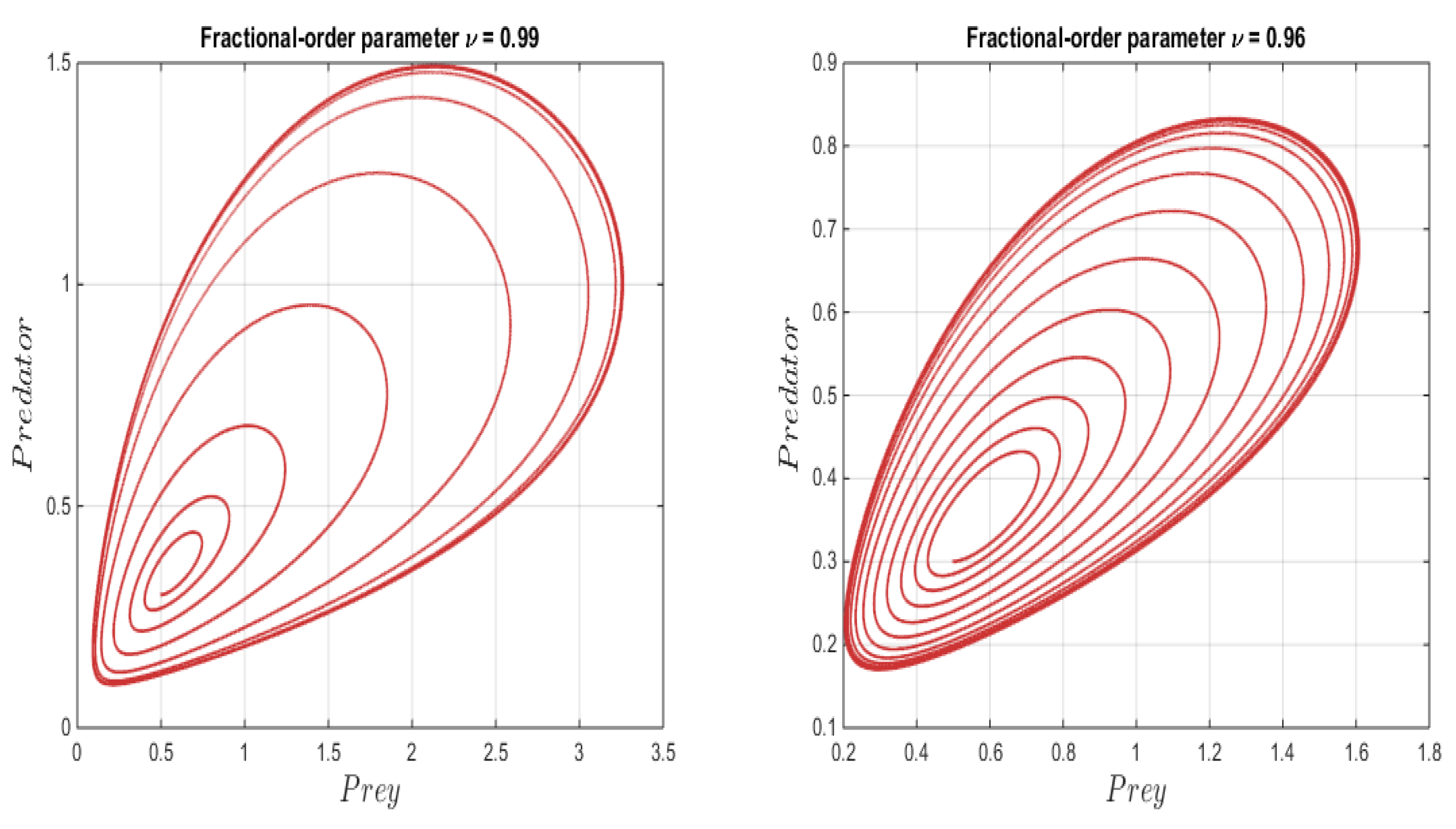
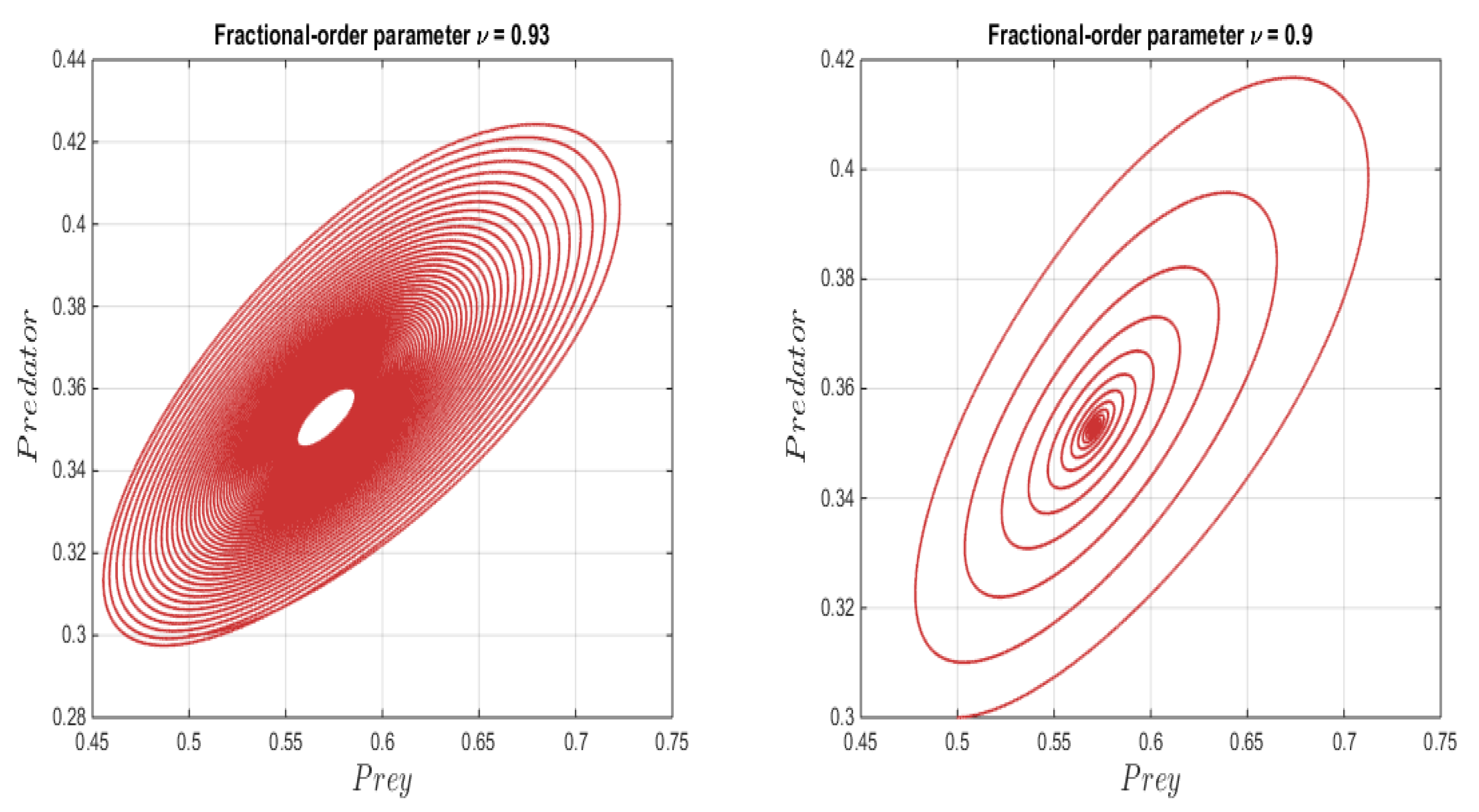
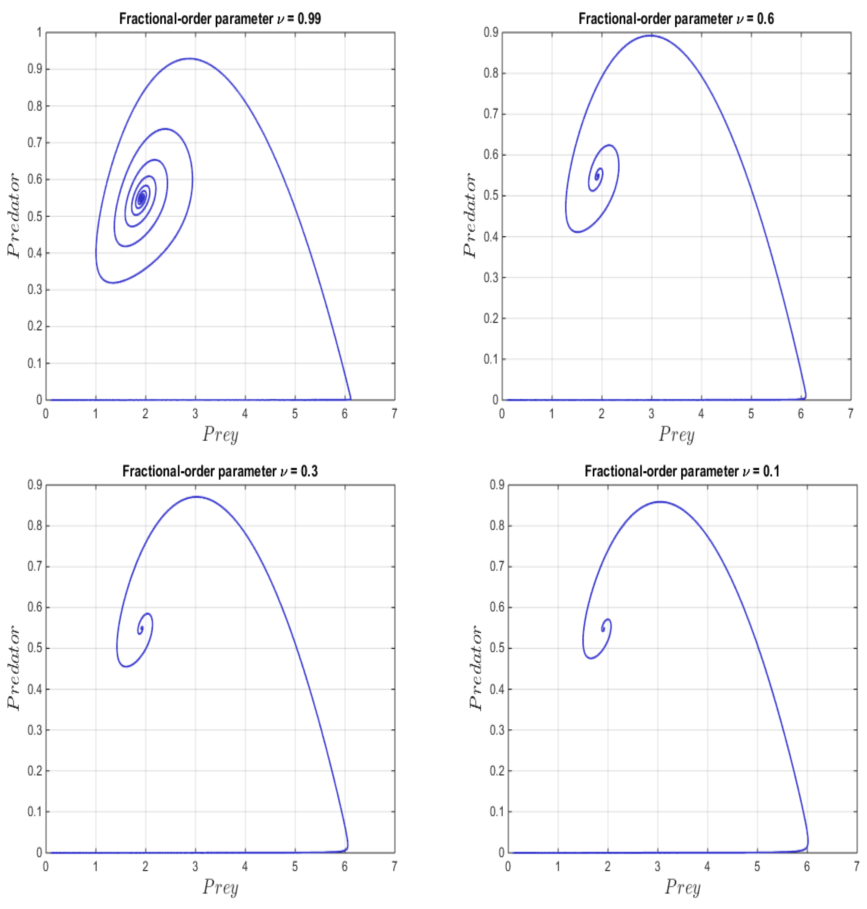
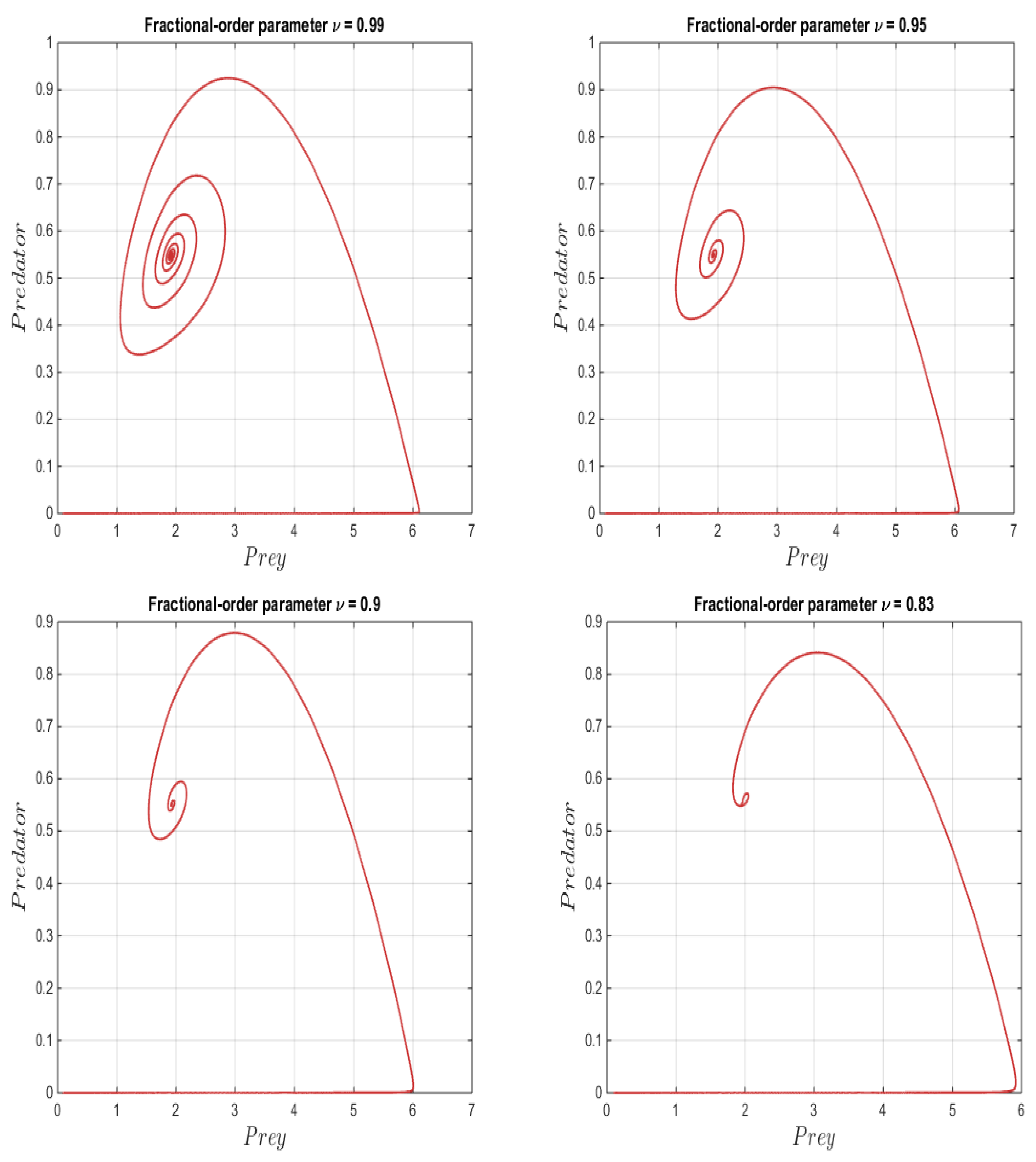
The initial conditions (ICs) ${(x\left(0\right),y\left(0\right))}^T={(0.1,0.0001)}^T$ and the parameter set A are used to simulate the dynamics of System (6) with different fractional orders (see Figure 1), which involve four figures to explain the dynamical behaviors of System (6). When the fractional order is $\nu =0.99$, fluctuations are observed in the system; they then settle near the equilibrium point $(1.9,0.55)$. However, as the fractional order decreases, the fluctuations subside, as shown in the remaining sub-figures. From a biological perspective, the memory and hereditary properties provide the species with more experience based on past history, making the system more stable, as shown in this case. Another scenario of complex dynamics in System (6) is obtained using the ICs ${(0.5,0.3)}^T$ and the parameter set $B_1$ (see Figure 2). For the second set (i.e., set B1), we observe a state of instability compared to the first set (i.e., set A). This behavior is due to several factors influencing the system, such as the significant increase in predator capture rate and carrying capacity, the decrease in predator mortality despite the increased prey growth rate, and the reduced impact of climate change specifically on predators. 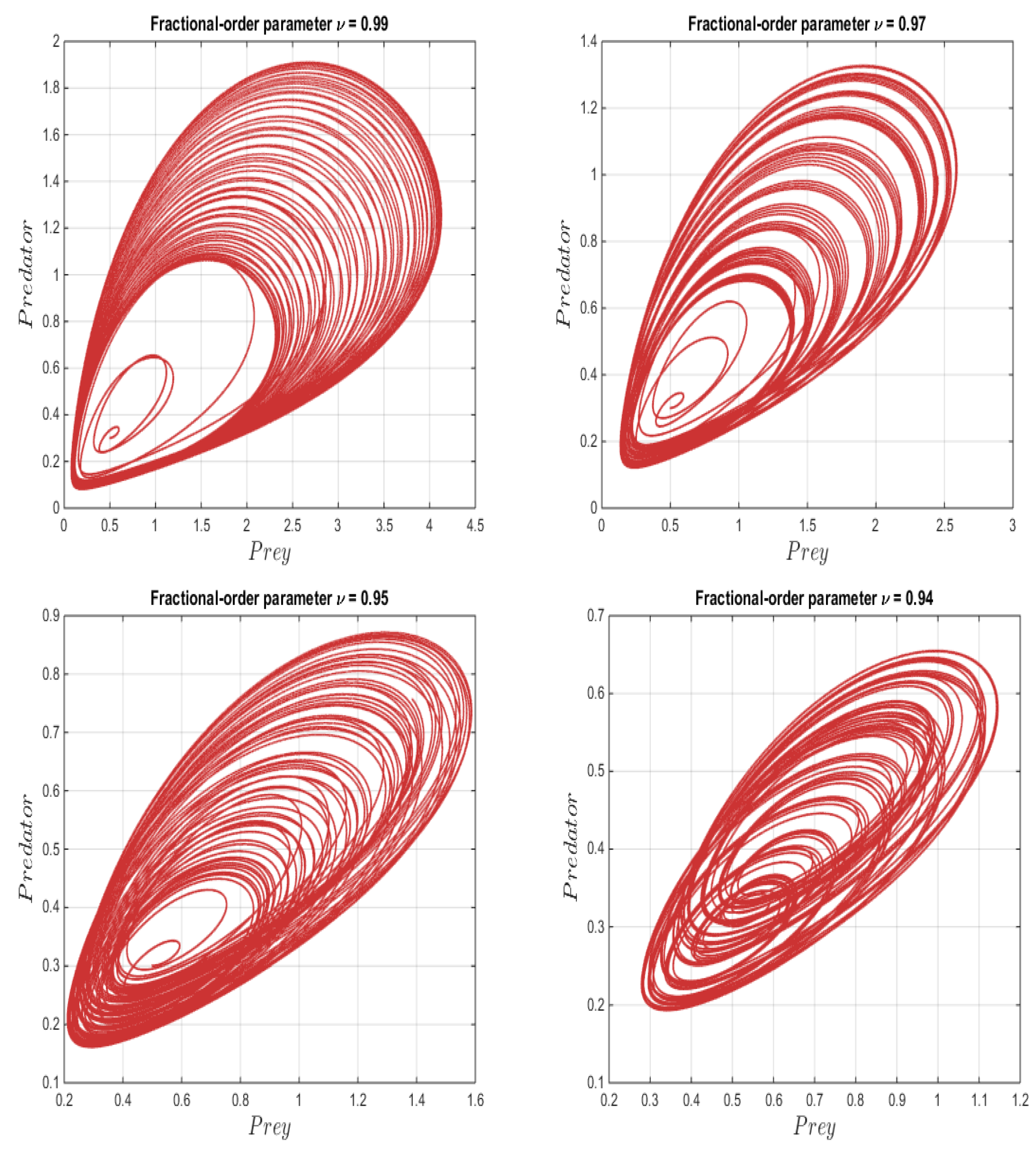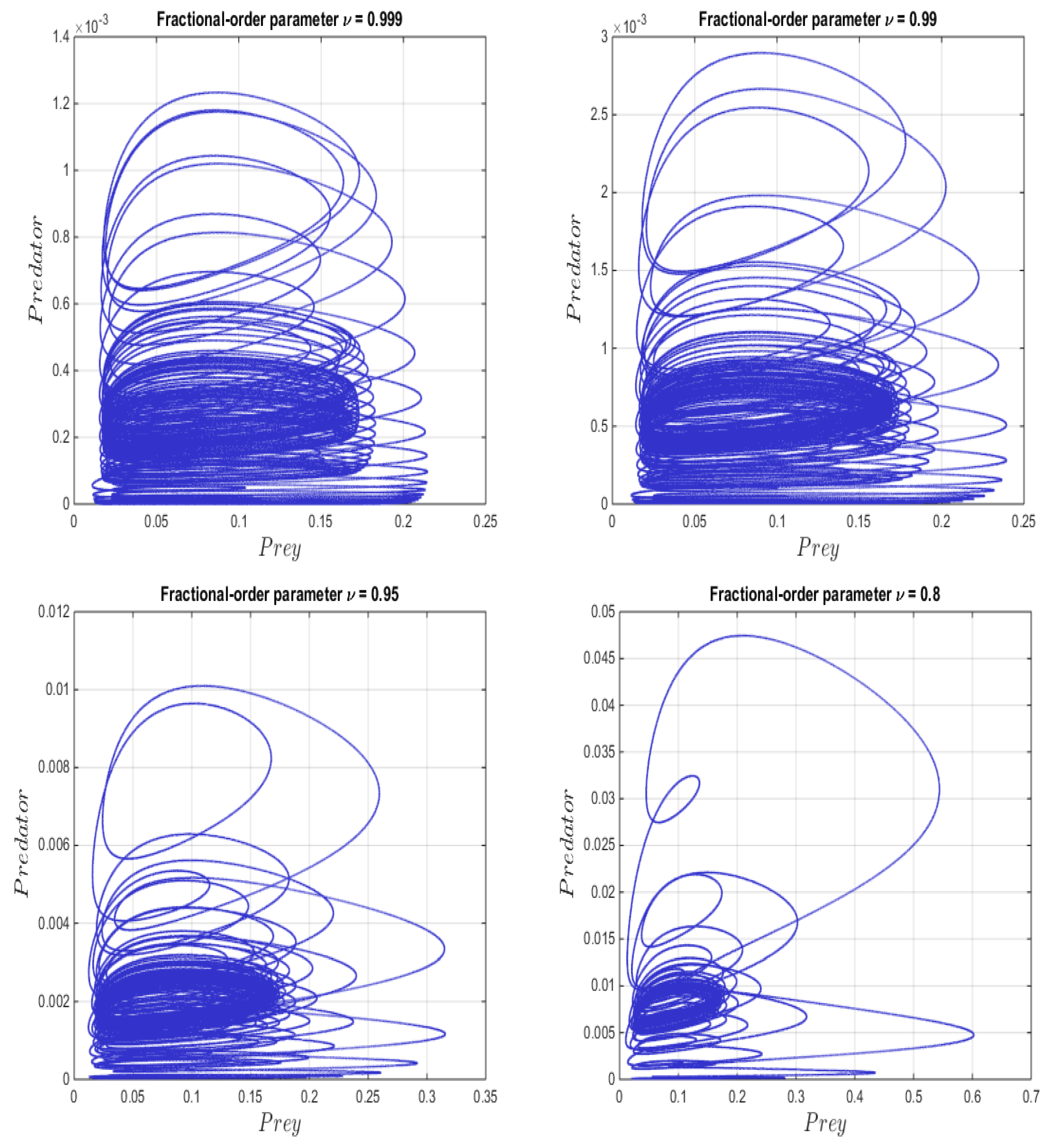Figure 2 shows an important change in dynamic behavior: when the fractional order is $\nu =0.99$, it shows unstable cycles as it approaches the axes. However, these cycles stabilize as the order decreases to reach a stable state, and this increases the probability of coexistence between species. However, the presence of memory and hereditary characteristics contributes to the system’s transition from an unstable state to a stable state, as illustrated in Figure 2.

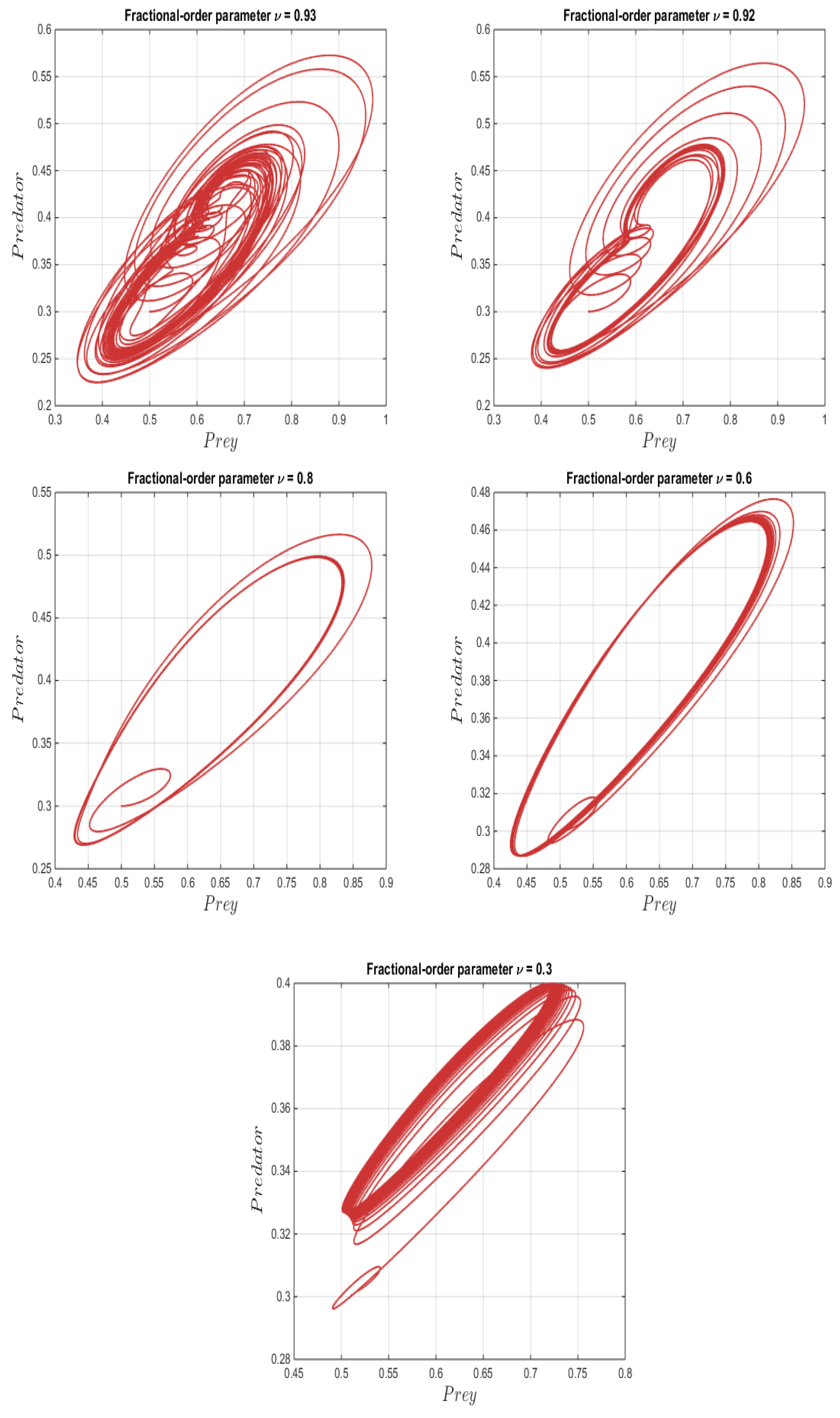
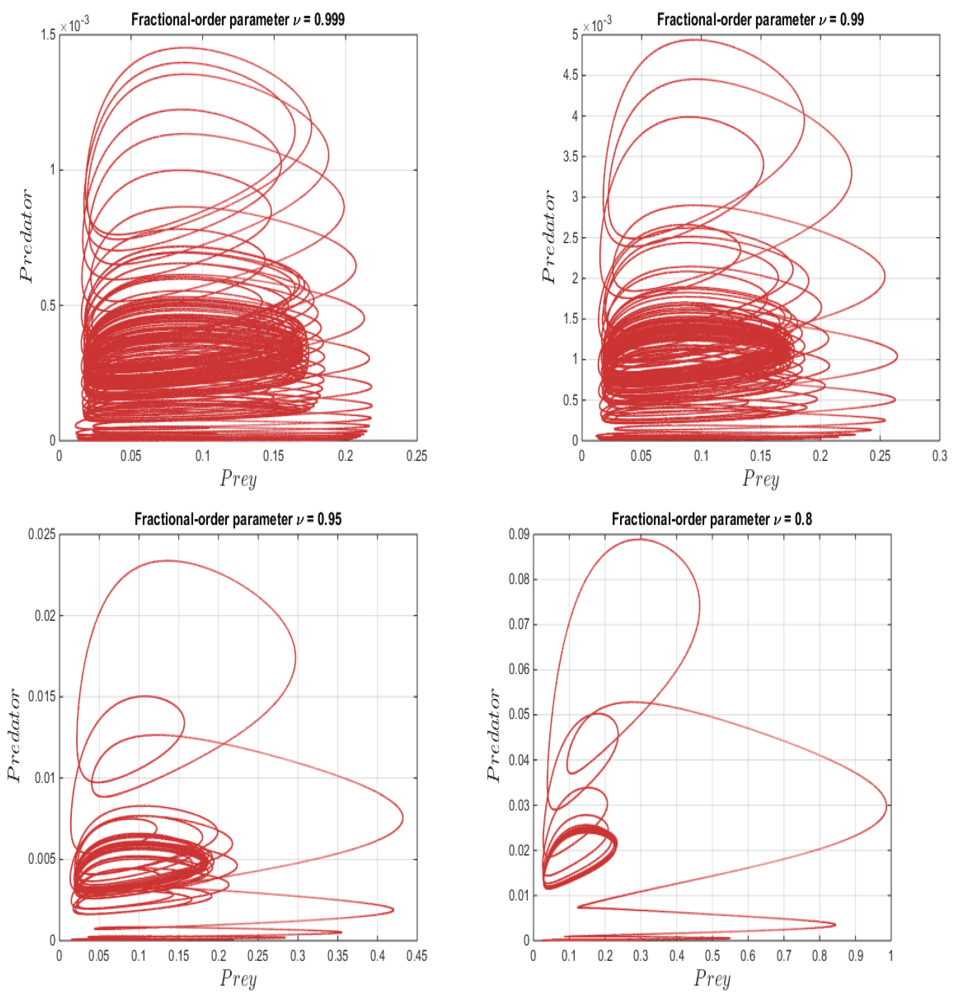
An interesting route to chaos in the nonautonomous system (System (7)) is observed when the parameter set $B_2$ is chosen with the ICs ${(0.5,0.3)}^T$. 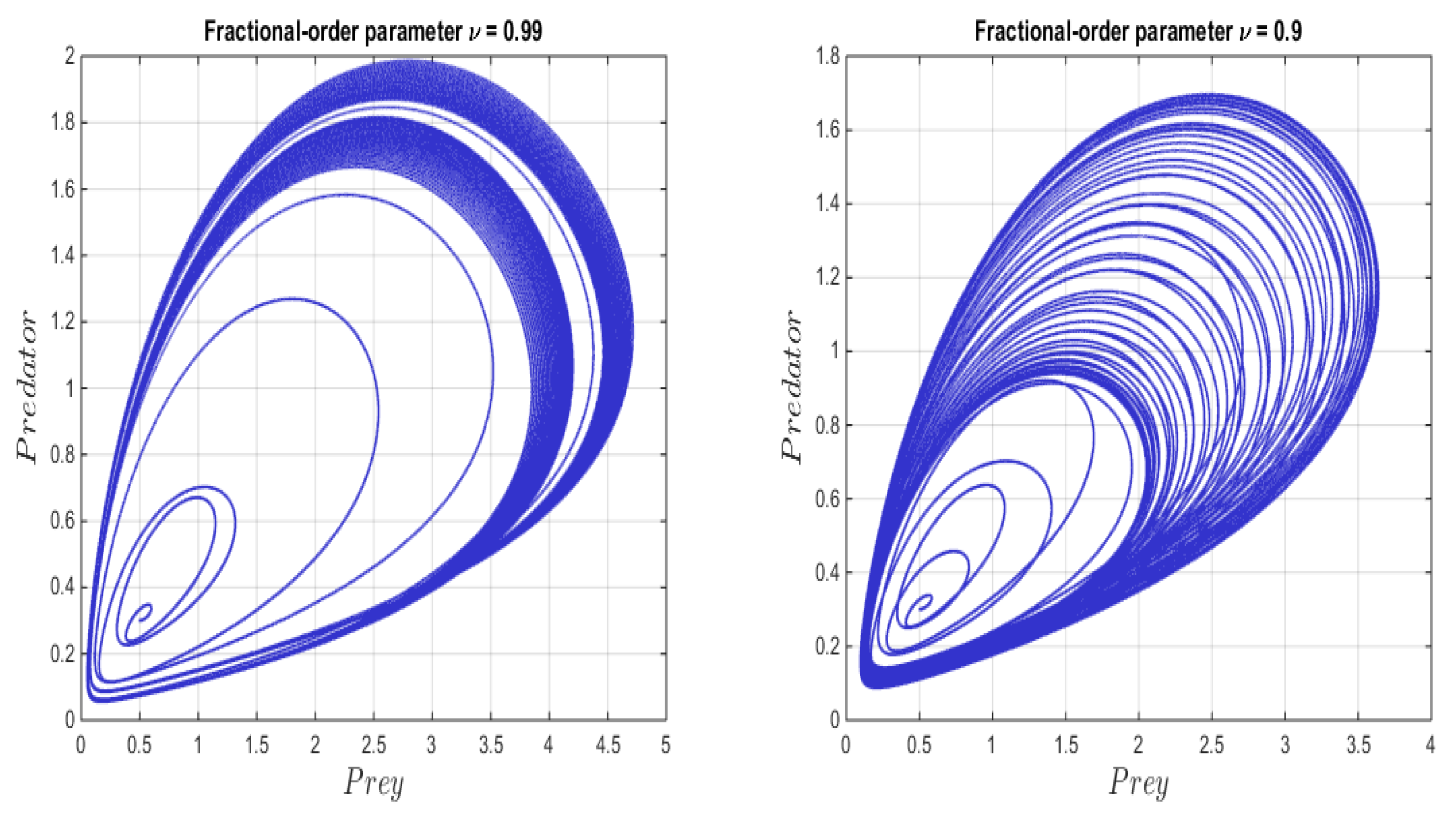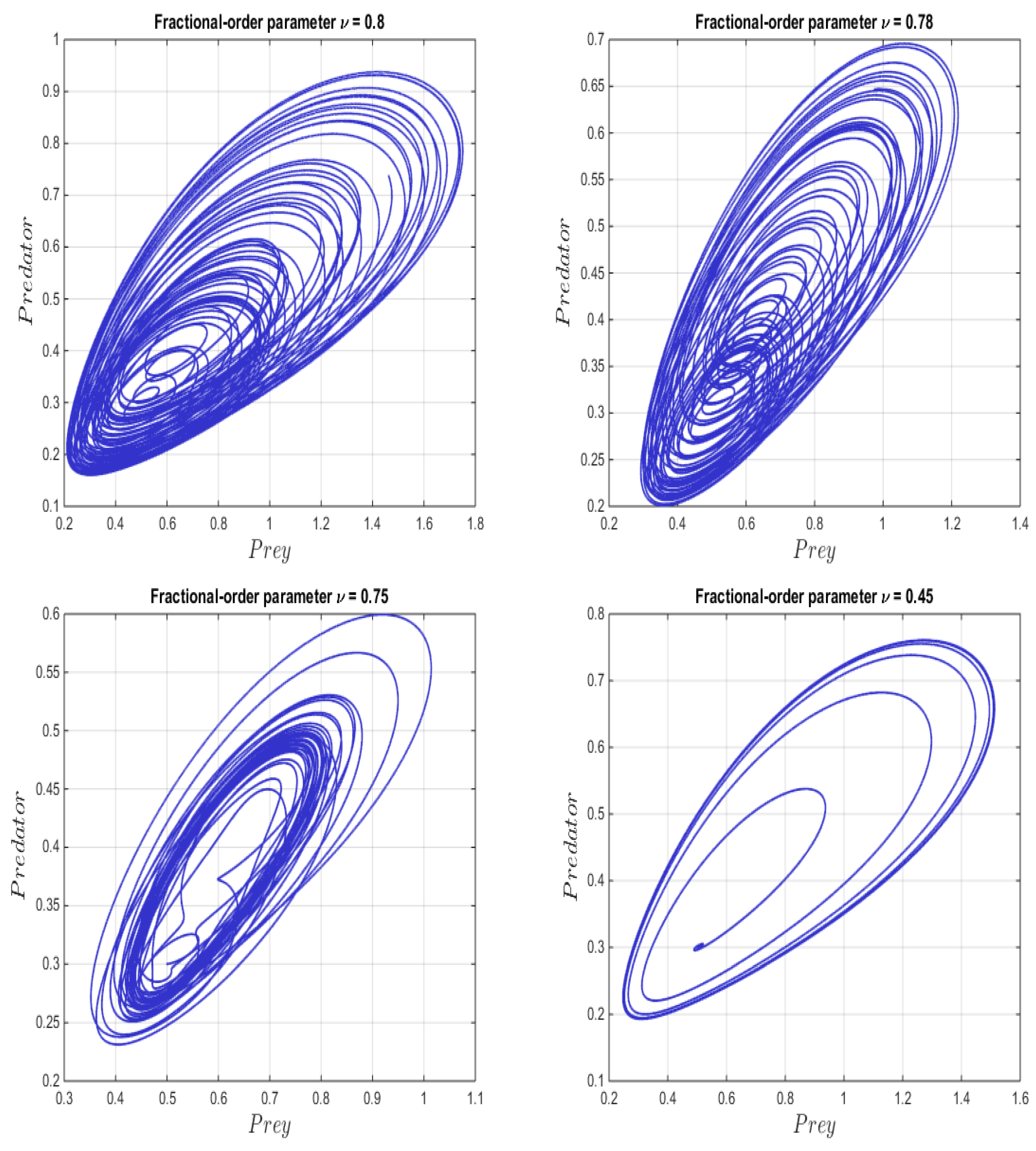One of the clearest indicators of climate change is the occurrence of seasonal variations over relatively short periods of time, representing realistic simulations of the seasonal environmental changes observed in natural ecosystems, and this is represented by the nonautonomous system (System (7)). This means that the coexistence of both the predator and prey populations is highly unpredictable because of the system’s high sensitivity under the initial conditions and the seasonality effects. Therefore, any small change will lead to drastic consequences on the oscillations of the species. These chaotic behaviors are clearly observed when $\nu =0.95$ and $0.94$. 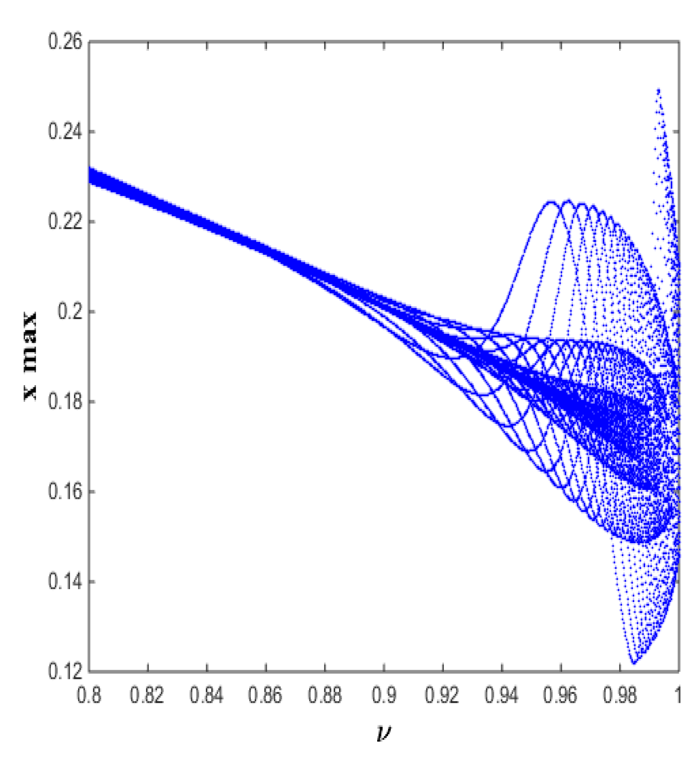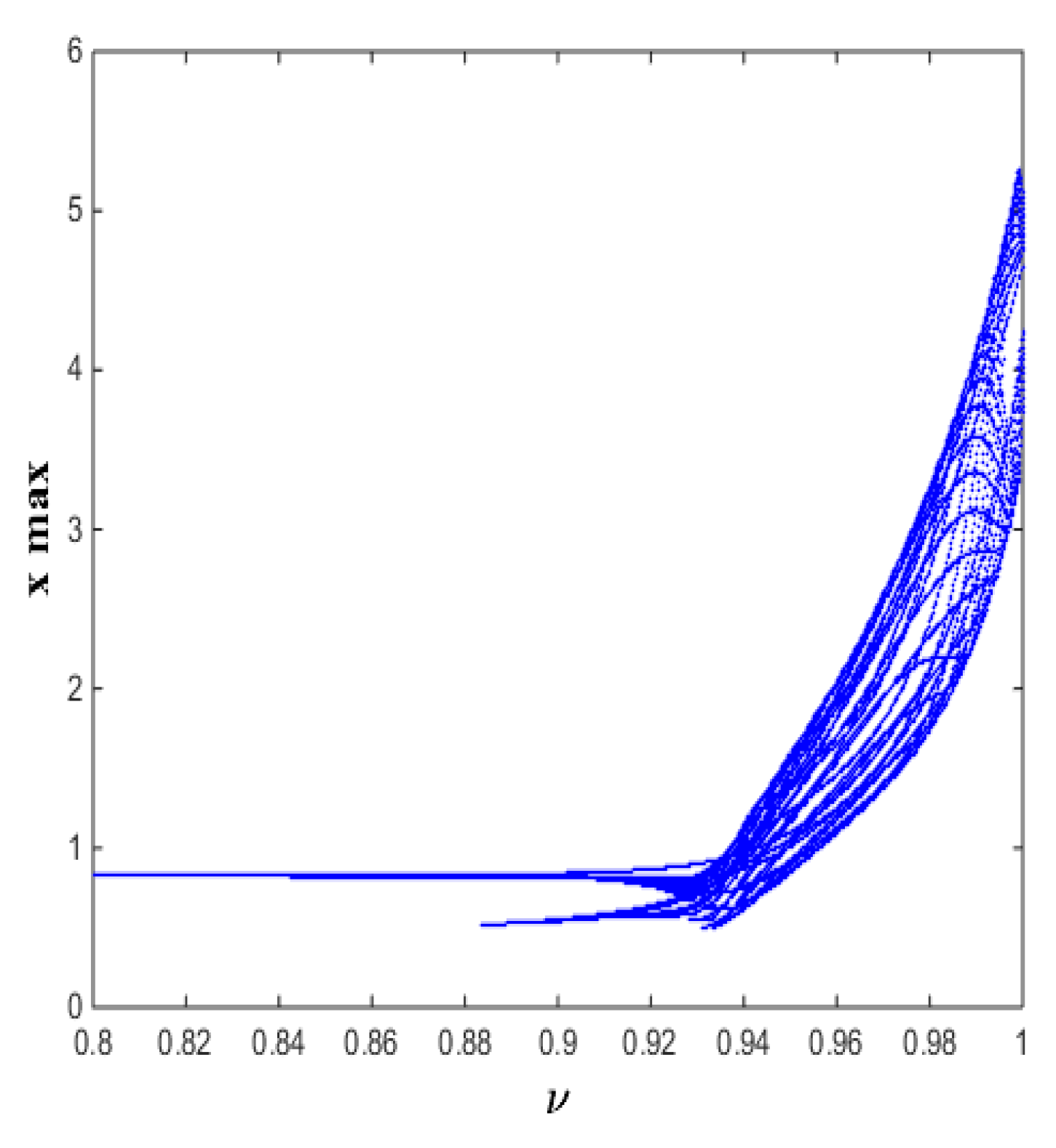When $\nu$ drops further to $0.93$, the system starts to lose its chaoticity, and approximate periodic oscillations are found, e.g., when $\nu =0.8,0.6$ and $0.3$ (see Figure 3). In addition, this route to chaos is outlined in the bifurcation diagram illustrated in Figure 4. When the parameter set C is chosen with the ICs ${(0.1,0.0001)}^T$, System (7) follows another route to chaos with different chaotic attractor shapes. When $\nu$ drops further to $0.9$, the system starts to lose its chaoticity, and approximate periodic oscillations are found, e.g. 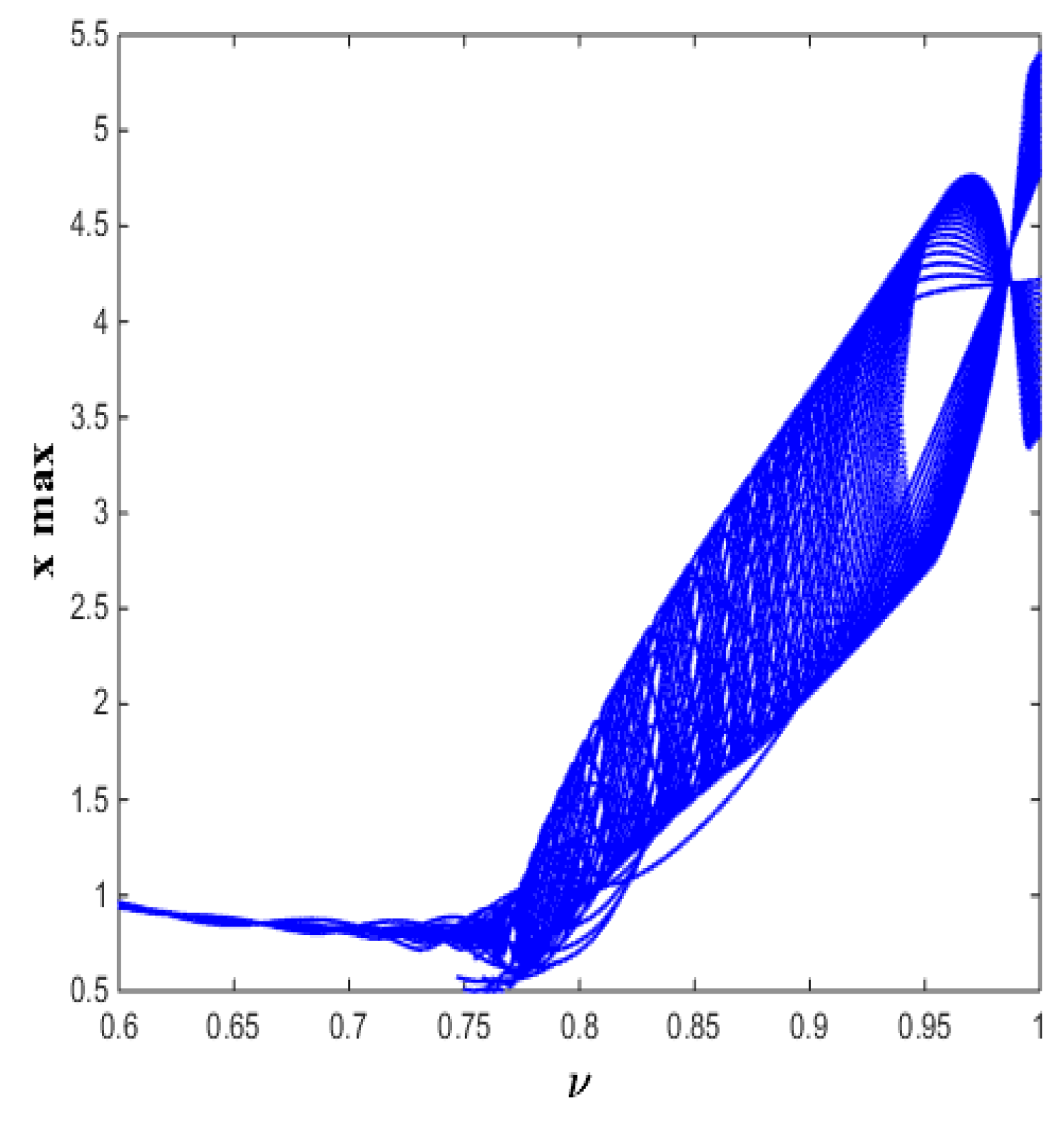when $\nu =0.8$ (see Figure 5). The corresponding bifurcation diagram is depicted in Figure 6, which shows that the fractional-order $\nu$ changes the dynamical behaviors of the model. In this case, it is observed that the system requires strong memory effects or more experienced species to adapt to such complex environmental conditions, necessitating reliance on past history. This can be explained by the complex dynamics involved in chaotic behavior, particularly in set C, which is characterized by strong climatic variations that affect prey species. Consequently, prey species need to modify their behavior, such as seeking new shelters to cope with harsh climatic conditions and avoiding predation by predators.

According to the algorithm [48], we calculate the Lyapunov exponents (LEs) for the system (7) using the parameter set $B_2$ and initial values ${(0.5,0.25)}^T$. The algorithm’s parameters are specified as follows: $tstart=0$, $tend=1000$, $hnorm=0.001$ and step size $h=0.01$. The calculated maximal Lyapunov exponents (MLEs) are given in

Table 2. The calculations of MLEs with different values of the fractional order.

Fractional Order $\mathit{\nu }$	MLE
$0.9$	$-0.00191187$
$0.92$	$-0.000338117$
$0.93$	$-0.000577398$
$0.94$	$0.00162203$
$0.95$	$0.00126432$
$0.96$	$0.000864443$
$0.97$	$0.00102383$
$0.98$	$0.00120976$

for different values of the memory parameter $\nu$ to demonstrate the transition between stable, quasi-periodic and chaotic dynamics in the considered system.

5.2. Simulation Results Using the CFO

To explain the numerical scheme, we consider the following general system governed by the CFO:

$${}^{CF}O_0^{\nu }\chi \left(t\right)=\mathsf{\Psi }(t,\chi \left(t\right)),\chi \left(0\right)={\chi }_0,$$

(13)

where $\mathsf{\Psi }$ denotes a non-linear vector function and $\chi$ represents the vector of the system’s state variables. Then, we obtain

$$\chi \left(t\right)={\chi }_0+(1-\nu )\mathsf{\Psi }(t,\chi \left(t\right))+\nu \underset{0}{\overset{t}{\int }}\mathsf{\Psi }(z,\chi \left(z\right))dz.$$

(14)

The discretization of Equation (14) is given by

$$\chi \left(t_{k+1}\right)={\chi }_0+(1-\nu )\mathsf{\Psi }(t_k,\chi \left(t_k\right))+\nu \underset{0}{\overset{t_{k+1}}{\int }}\mathsf{\Psi }(t,\chi \left(t\right))dt,$$

(15)

where k represents a non-negative integer. Equation (15) can be reformulated as

$$\chi \left(t_k\right)={\chi }_0+(1-\nu )\mathsf{\Psi }(t_{k-1},\chi \left(t_{k-1}\right))+\nu \underset{0}{\overset{t_k}{\int }}\mathsf{\Psi }(t,\chi \left(t\right))dt.$$

(16)

Based on Equations (15) and (16),

$$\chi \left(t_{k+1}\right)=\chi \left(t_k\right)+(1-\nu )\left(\begin{array}{c}\mathsf{\Psi }(t_k,\chi \left(t_k\right))-\mathsf{\Psi }(t_{k-1},\chi \left(t_{k-1}\right))\end{array}\right)+\nu \underset{t_k}{\overset{t_{k+1}}{\int }}\mathsf{\Psi }(t,\chi \left(t\right))dt,$$

(17)

given that

$$\underset{t_k}{\overset{t_{k+1}}{\int }}\mathsf{\Psi }(t,\chi \left(t\right))dt=\left(\begin{array}{c}{\displaystyle \frac{3}{2}}\mathsf{\Psi }(t_k,{\chi }_k)-{\displaystyle \frac{\mathsf{\Psi }(t_{k-1},{\chi }_{k-1})}{2}}\end{array}\right)h,$$

(18)

where h represents the step size. Finally, we obtain

$$\chi \left(t_{k+1}\right)=\chi \left(t_k\right)+({\displaystyle \frac{3\nu h}{2}}+1-\nu )\mathsf{\Psi }(t_k,{\chi }_k)-({\displaystyle \frac{\nu h}{2}}+1-\nu )\mathsf{\Psi }(t_{k-1},{\chi }_{k-1}).$$

(19)

According to Ref. [49], the error estimate of this numerical scheme is given by

$$\left|E\left(\mathsf{\Psi }\right)\right|\le \nu k{h}^3,$$

(20)

where $k=-{\displaystyle \frac{7}{12}}{\mathsf{\Psi }}^{\left(2\right)}(t,\chi ).$ Moreover, this numerical scheme has been proven to be conditionally stable and conditionally convergent in Theorems 2 and 3 of Ref. [49], respectively.

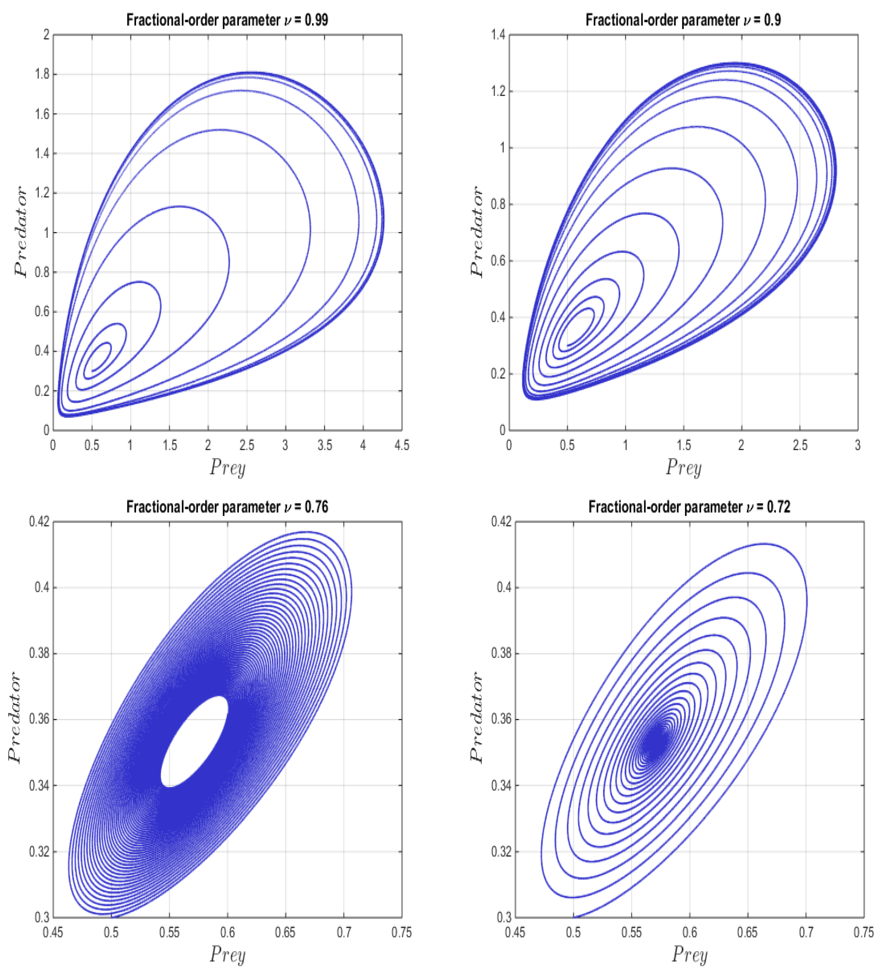
Here, the considered systems are integrated using the above-mentioned numerical scheme with $h=0.01$ and $N=\mathrm{100,000}$. The ICs ${(0.1,0.0001)}^T$ and the parameter set A are used to simulate System (6) with different values of $\nu$, as shown in Figure 7, which reveals that the populations do not spiral in an uncontrollable manner because all the system’s trajectories converge to the stable interior equilibrium. So, the prey and predator populations can sustain themselves over a long time course and long-term memory, thereby enhancing the system’s stability. A route to periodic dynamics is obtained in System (6) using the ICs ${(0.5,0.3)}^T$ and the parameter set $B_1$, as shown in Figure 8. Here, limit cycles, which occur through Hopf bifurcations, are obtained for a wider range of parameters, and the memory parameter $\nu \in [0.8,0.99]$ is compared against the system’s counterpart governed by the CO. This periodic solution is created near $\nu =0.75$, indicating that both the predator and prey species will repeatedly rise and fall in a regular, predictable pattern of dynamical behaviors. When $\nu$ further drops to $0.72$, the system starts to lose its periodicity, and asymptotically stable attractors are observed. Memory effects and hereditary properties play significant roles in stabilizing the system dynamics, enabling the system to evolve from instability toward a stable equilibrium, as demonstrated in Figure 8.

Subsequently, when the parameter set $B_2$ is selected with the ICs ${(0.5,0.3)}^T$ in System (7), the chaotic attractors appear on a wider scale of the memory parameter $\nu \in [0.75,0.93]$ compared to the system’s counterpart governed by the CO. Unlike the CO version, chaos disappears when $\nu$ approaches one. Moreover, when $\nu$ further drops to $0.75$, the chaotic dynamics diminish and are replaced with quasi-periodic and periodic attractors. 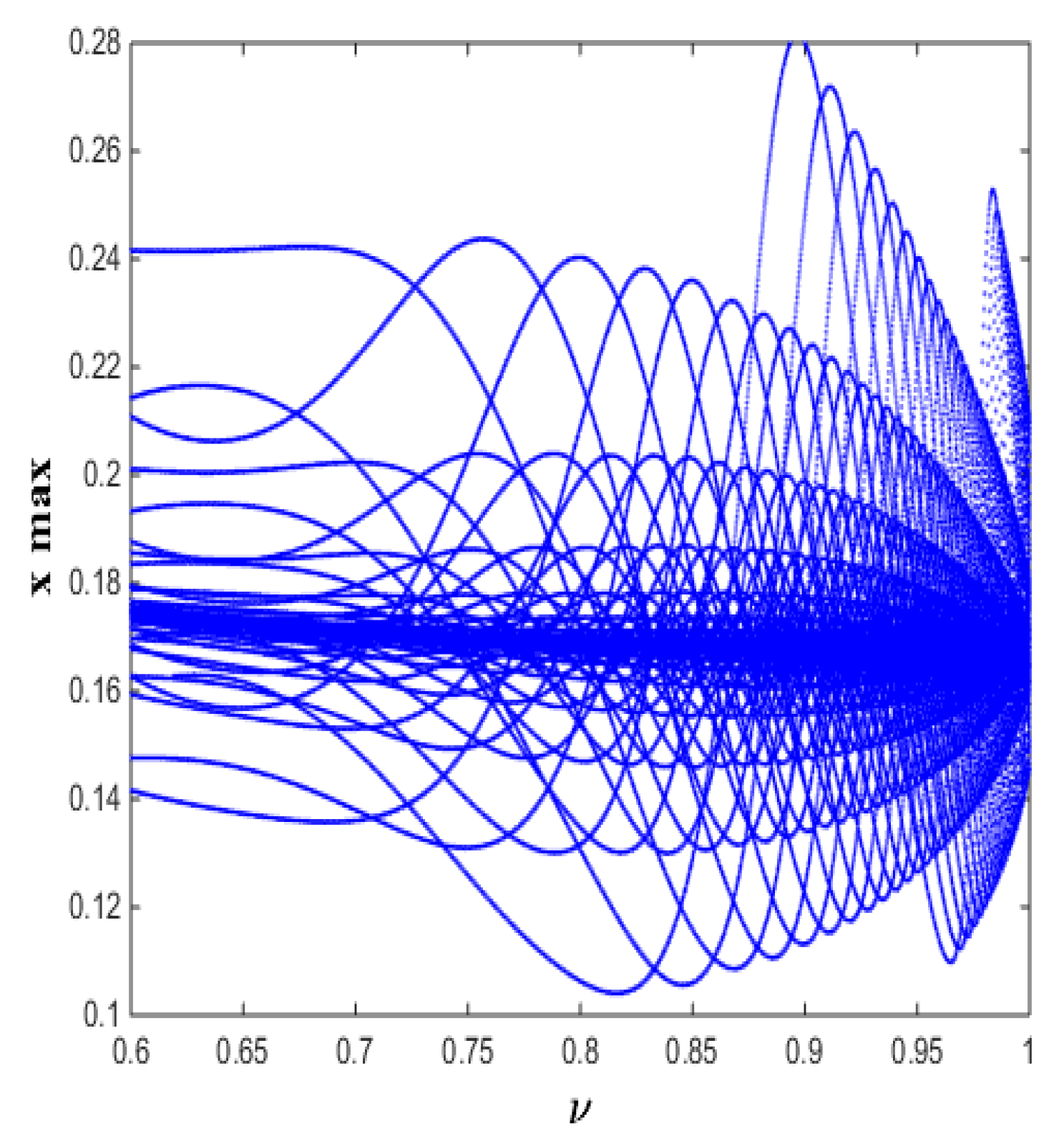This scenario is illustrated in Figure 9 and summarized in the bifurcation diagram in Figure 10. In Figure 10, the chaotic states are observed when the memory parameter $\nu$ exceeds 0.75 and transitions from chaotic states to quasi-periodic states, and they are also observed when $\nu$ exceeds 0.95. When comparing the previous bifurcation diagram with the bifurcation diagram in Figure 4, we find that the chaos scenario starts later in the CO case, approximately after the memory parameter crosses 0.93, and ends at approximately one. Therefore, it is a relatively shorter scenario than the CFO case, as shown in Figure 10.

On the other hand, when the parameter set C is selected with the ICs ${(0.1,0.0001)}^T$, System (7) exhibits different patterns of chaotic dynamics, as shown in Figure 11. Thus, the chaotic attractors in this case appear on a wider scale of the fractional-order $\nu$ compared to the system’s counterpart governed by the CO. A bifurcation diagram is drawn in Figure 12 to illustrate this interesting scenario of chaotic dynamics.

It is observed that the Caputo–Fabrizio operator exhibits slower transitions between different dynamical states compared to the Caputo operator, resulting in more gradual and less abrupt changes. This explains the richer presence of complex dynamics, and this behavior is attributed to the operator itself, which possesses short-term or fading memory due to the exponential kernel involved in its formulation [50].

In the following remark, we introduce some ecological interpretations:

Remark 6.

The shift from chaotic dynamics and periodic fluctuations to more stable dynamics can be ecologically attributed to the existence of prey refuge and greater prey abundance for predators, and these strategies can contribute to species survival and conservation. The presence of memory can influence prey behaviors and the development of shelter strategies to avoid being caught by predators, and it can also affect the effectiveness of predator hunting by relying on the historical presence of prey [42].

6. Biological Significance and Limitations of the Proposed Fractional Models

The considered Holling type II PP models under climate change effects provide distinguishable insights into the intricate relationship between the predator and the prey populations. In addition, they show the impact of memory and hereditary properties on the species by providing them with more experience based on past history, making the model more stable when static climate changes are considered. According to Theorem 1, both the prey and predator species become extinct over time, as they start from zero, when the memory parameter $\nu$ satisfies the condition ${\displaystyle \frac{1}{1-\nu }}<\gamma -e_1$. However, the prey and predator species do not go extinct when the prey’s inherent growth rate lies in $(e_1,e_1+{\displaystyle \frac{1}{1-v}})$. Based on Condition (iv) of Lemma 3, it is found that the predator species is biologically doomed to extinction, while the prey species stabilizes at its own carrying capacity when the memory parameter $\nu <$${\displaystyle \frac{2\left|{tan}^{-1}\left(\sqrt{4{\rho }_2-{\rho }_1^2}\right)/{\rho }_1\right|}{\pi }}$, ${\rho }_1<0,$ and $4{\rho }_2>{\rho }_1^2$.

Condition (iv) of Lemma 4 implies that when the memory parameter $\nu <1-{\displaystyle \frac{1}{-\xi -e_2+\frac{E\sigma C(\gamma -e_1)}{\gamma +\gamma H\sigma C(\gamma -e_1)}}}$, the predator is biologically doomed to extinction, while the prey stabilizes at its own carrying capacity if the system’s carrying capacity is less than half and the inherent growth rate of the prey is less than the climate change effect on prey species, and vice versa. However, the predator can successfully invade the environment when $\nu >1-{\displaystyle \frac{1}{-\xi -e_2+\frac{E\sigma C(\gamma -e_1)}{\gamma +\gamma H\sigma C(\gamma -e_1)}}}$ if the system’s carrying capacity is less than half and the inherent growth rate of the prey is less than the climate change effect on prey species, and vice versa.

When the memory parameter $\nu$ satisfies Conditions (4) and (5) of Lemma 6, the ecosystem achieves stable coexistence or long-term balance. However, the system’s balance is precarious when it pushes the predator and prey species away from that balance and the memory parameter $\nu$ satisfies Condition (6) of Lemma 6.

On the other hand, it is found that the species require strong memory effects or more experience to adapt to the complex environmental conditions when seasonal variations over relatively short periods of time occur, resulting in seasonal environmental changes in the natural ecosystems. In addition, various complex dynamics such as chaotic states are observed under certain circumstances and as the memory parameter gradually approaches one, meaning that strong climate variations affect the prey populations. Therefore, the prey population needs to modify its behaviors, for example, by seeking new shelters to cope with harsh climatic conditions and avoiding predation. This scenario of complex dynamics appears more broadly in the CFO case.

One of the major limitations of such studies is the relation of the resulting dynamics to biological interpretations. This arises from the complexity of predator–prey interactions in the environment and the presence of numerous influencing factors, which make these dynamics difficult to formulate and follow mathematically. In addition, numerical simulations of fractional predator–prey systems require relatively high computational effort. In future work, this model can be extended using the Beddington–DeAngelis and Crowley–Martin functional responses, and it can also be generalized by incorporating additional environmental factors such as prey shelters, immigration, and other ecological effects. Furthermore, periodic or oscillatory solutions can be studied and analyzed in more detail.

7. Conclusions

This study examined the impact of memory effects on complex dynamics in predator–prey models under static and periodic climate change, and Holling type II functional responses and the Caputo and Caputo–Fabrizio fractional operators are used to formulate fractional predator–prey models. The stability analysis of all equilibrium states is conducted in the framework of each fractional-order operator employed.

The obtained results conclude that climate change effects and memory and hereditary properties play a significant role in determining the long-term dynamics of the predator–prey system. The analytical results show that, under both singular and nonsingular kernels, the relationship between the prey’s intrinsic growth rate and the climate change effect determines whether the populations move toward extinction or coexistence; when the prey growth rate is insufficient to overcome environmental stress, both prey and predator populations eventually vanish. In contrast, increasing the prey growth rate beyond the critical thresholds allows the system to avoid extinction and promotes the possibility of population recovery and coexistence.

Furthermore, the stability analysis demonstrates that the carrying capacity, climate change, and strength memory effects strongly influence the stability state, as well as extinction and coexistence dynamics. The results indicate that predators may become biologically extinct, while preys stabilize at their carrying capacity under certain parameter conditions. However, increasing the carrying capacity and adjusting the growth conditions can enable predator invasion and lead to stable coexistence between the two species. Also, prey growth is subject to climatic changes and memory strength, which remain stable within a certain period; otherwise, the dynamic behavior is unstable.

Numerical simulations demonstrate a variety of complex dynamics with both operators. Comparative numerical results reveal that for the second model, the Caputo–Fabrizio operator yields chaotic regimes over wider parameter ranges than those obtained using the Caputo operator, indicating a richer representation of complex dynamics. On the other hand, it is found that the species require strong memory effects or more experience to adapt to the complex environmental conditions when seasonal variations over relatively short periods of time occur, resulting in seasonal environmental changes in the natural ecosystems. In addition, several complex dynamics, such as chaotic states, are observed under certain circumstances and as the memory parameter gradually approaches one, indicating that strong climate variations affect the prey populations. The numerical results also show an improvement in species stability and thus an increased probability of survival under adverse climatic conditions through the presence of memory effects.

One of the major limitations of such studies is linking the obtained dynamical behaviors to realistic biological interpretations. This difficulty arises from the complexity of predator–prey interactions in natural environments and the presence of numerous ecological factors that influence the system, making the dynamics mathematically challenging to formulate and analyze. Moreover, numerical simulations of fractional predator–prey models generally require considerable computational effort.

As a direction for future research, the present model can be extended by incorporating other functional responses, such as the Beddington–DeAngelis and Crowley–Martin types. The model may also be generalized by including additional ecological and environmental factors, such as prey shelters, immigration, and other biological effects. Furthermore, periodic and oscillatory solutions of the system can be investigated and analyzed in more detail.