Topological Machine Learning Framework for Phase Portrait Classification of Nonlinear Dynamical Systems

Abstract

Nonlinear dynamical systems exhibit complex behaviors such as periodicity and chaos, which are traditionally analyzed using time-series data. However, these approaches often fail to capture the intrinsic geometric structure of the system dynamics represented in the phase space. In this study, we address this limitation by proposing a topological machine learning framework that leverages phase portrait images to classify dynamical regimes. The primary objective of this study is to investigate whether the topological features extracted from phase portraits can effectively distinguish between periodic and chaotic behaviors across different nonlinear systems. To achieve this, we employed the Topological Data Analysis (TDA) technique of cubical homology, which enables the extraction of topological descriptors, such as persistence diagrams and Betti curves. We used these features to train multiple machine learning (ML) classifiers, including XGBoost, Support Vector Machine (SVM), K-Nearest Neighbors (KNN), Gaussian Naïve Bayes (GNB), and Random Forest (RF). The experimental results across benchmark systems, including the Chua, Lorenz, Mathieu–Duffing, and erbium-doped fiber laser models, demonstrate that the proposed approach achieves high classification accuracy, with performance improving from approximately 93% under $H_0$ features to 99–100% under $H_1$ and combined feature representations. These findings highlight that topological features, particularly $H_1$, effectively capture the underlying geometric structure of dynamical systems. Overall, the proposed framework provides a robust, interpretable, and generalizable approach for phase portrait classification, with potential applications in nonlinear system analysis, pattern recognition, and early detection of chaotic transitions.

1. Introduction

Nonlinear dynamical systems are widely used to describe complex phenomena observed in physics, engineering, biology, and many other scientific fields. One of the most intriguing characteristics of nonlinear systems is their ability to exhibit chaotic behavior, characterized by sensitivity to initial conditions, irregular temporal evolution, and unpredictability. Chaotic dynamics appear in many natural and engineering systems, such as lasers [1], electrical circuits [2], and chemical reactions [3]. Chaotic systems are used in data security applications [4] and encryption [5,6] owing to their inherent randomness.

Time-series analysis has long been the primary approach for studying dynamical systems, providing valuable insights into their temporal evolution and enabling the investigation of behaviors such as periodicity, bifurcations, and transitions to chaos [7]. Classical nonlinear tools, including Lyapunov exponents, bifurcation diagrams, Poincaré maps, and Fourier spectral analysis, are widely used to characterize these dynamics [8]. However, these methods primarily focus on the evolution of individual state variables and may not fully capture the intrinsic geometric relationships among multiple variables. Therefore, phase portraits (PPs) have gained increasing attention, as they offer a geometric representation of the system in its phase space [9]. A phase portrait reveals the qualitative structure of the dynamics by illustrating features such as fixed points, periodic orbits, quasi-periodic motion, and chaotic attractors, the latter often forming intricate patterns known as strange attractors. Moreover, PPs can be interpreted as images containing rich visual patterns, which has led to their growing use in modern computational approaches, including machine learning and neural networks [10]. In chaotic systems, a small change in the control parameter can produce subtle yet significant variations in the attractor geometry, making phase portrait-based analysis both challenging and highly informative.

The limited exploration of PPs in dynamical system analysis motivated this study to examine them based on their pixel-based structures. To address these challenges, this study employs Topological Data Analysis (TDA) to extract geometric and topological features from PPs. In particular, persistent homology (PH) captures features such as connected components and loops across multiple scales [11,12]. For image-based data, cubical homology (CH) provides a computationally efficient framework by directly modeling images as pixel-based cubical complexes [13]. Unlike simplicial-complex-based approaches, which generally require triangulation or point cloud construction, CH naturally preserves the grid structure of two-dimensional images and enables efficient filtration for topological feature extraction. The resulting persistence diagrams (PDs) [14] are transformed into descriptors, such as Betti curves, enabling effective integration with machine learning (ML) models.

Many ML methods, such as support vector machines, k-nearest neighbors, and neural networks, have been widely applied to time-series data [15,16], but they often overlook the intrinsic geometry of attractors. Recent studies have explored deep learning-based classification of chaotic systems using phase portrait and attractor images, achieving high classification accuracy across different nonlinear systems [17,18]. Deep learning approaches applied to PPs [19] show promise but typically require large datasets and do not explicitly capture structural properties. However, these approaches primarily rely on pixel-level feature learning and generally require large datasets while providing limited interpretability regarding the intrinsic geometric structure of the attractors. In contrast, the proposed TDA-based framework directly captures the topological shape characteristics of phase portraits, such as connected components and loop structures, enabling a more interpretable and geometry-driven analysis of nonlinear dynamical behaviors.

Although TDA has been successfully applied to dynamical systems, to detect P-type bifurcations in stochastic dynamical systems using superlevel persistence [20]. Another study by [21] mainly focused on PH to detect bifurcations and the onset of chaos by extracting topological features from nonlinear time-series data. CH has also been successfully applied to several image-based applications, including hurricane pattern analysis [22], MRI image classification [23], and to estimate bone strength from micro-CT [24], due to its natural suitability for pixel-based image structures rather than direct time-series representations. However, the application of TDA to phase portrait images, particularly in combination with CH and ML, remains relatively underexplored. This study presents the application of CH to phase portrait images for the topological classification of nonlinear dynamical behaviors. This study highlights the potential to bridge the gap between geometric analysis and data-driven methods in chaos research.

Existing approaches for phase portrait analysis primarily utilize conventional machine learning or deep learning frameworks to extract pixel-level or learned feature representations. While these methods often demonstrate strong classification performance, they typically require large datasets and offer limited interpretability concerning the geometric organization of nonlinear attractors. In contrast, the proposed framework utilizes cubical homology-based topological descriptors to directly characterize the structural properties of phase portraits through connectivity and loop evolution. This approach yields a geometry-driven and interpretable representation for nonlinear dynamical classification.

Motivated by these observations, this study investigates the use of TDA to extract structural features from phase portrait images of dynamical systems. This approach bridges the gap between the geometric features of PPs and ML techniques by extracting topological shape descriptors for classification. Accordingly, the key contributions and overall significance of this study are summarized as follows:

• Topological machine learning framework: A novel framework is developed that bridges the gap between phase portrait geometric structures and machine learning by incorporating topological data analysis (TDA).
• Topological feature extraction from phase portraits: We extract topological signatures from phase portraits, such as persistence diagrams and ML features including Betti curves, by applying cubical homology.
• Beyond time-series based classification: This study shifts the focus from traditional single-variable time-series analysis to multi-variable relationships in phase space, enabling a more comprehensive understanding of dynamic system behavior.
• Efficient classification of dynamical regimes: The extracted topological descriptors serve as informative features for ML models to effectively classify the system’s dynamic behaviors, including periodic and chaotic regimes.

The proposed topological ML pipeline first converts phase portrait images into cubical complexes, from which the PH is computed to extract the multi-scale topological features. In particular, the homological dimensions $H_0$ and $H_1$ correspond to connected components and loop structures, respectively, and are further characterized by Betti curves. Multiple ML classifiers, including XGBoost, SVM, KNN, Gaussian Naïve Bayes, and Random Forest, are employed to distinguish between periodic and chaotic regimes. To evaluate the discriminative capability of the extracted features, t-SNE visualization and confusion matrix analysis are performed. Experimental results obtained from nonlinear systems, including the Chua, Lorenz, Mathieu–Duffing, and erbium-doped fiber laser models, demonstrate that the proposed framework achieves high classification accuracy, particularly when using $H_1$ and combined feature representations. These findings indicate that topological descriptors effectively capture the intrinsic geometric structure of PPs and provide an interpretable framework for classifying dynamical behavior.

The remainder of this paper is organized as follows. Section 2 introduces the nonlinear dynamical systems considered in this study, including a detailed description of their governing equations and the procedure used to generate phase portrait representations. Section 3 provides the theoretical foundation of the CH and highlights its role in extracting topological features from image-based data. Section 4 presents the complete topological ML pipeline, including feature extraction, preprocessing, and classification methodologies. Section 5 reports the experimental results, including quantitative evaluation, visualization through t-SNE, and confusion matrix analysis, along with a comprehensive discussion of the findings. Finally, Section 6 summarizes the main contributions of this study and outlines the potential directions for future research.

2. Dynamical Systems and Phase Portraits Datasets

In nonlinear dynamical systems, phase portraits (PPs) play a fundamental role by providing a geometric representation of the system’s behavior in the state space. Rather than analyzing only numerical time series, PPs allow us to visualize the evolution of a system over time and the trajectories’ movement within the state space. A nonlinear dynamical system is commonly described by a system of differential equations

$$\dot{\overrightarrow{x}}=\overrightarrow{f}(\overrightarrow{x},t)$$

(1)

where $x\in {\mathbb{R}}^n$ denotes the state vector of the system and $f\left(x\right)$ represents a nonlinear function governing the system dynamics. A phase portrait is a graphical representation of the system’s trajectories in phase space.

2.1. Lorenz System

The Lorenz system is a nonlinear dynamical system consisting of three coupled equations, well known for exhibiting chaotic behavior. Edward Lorenz proposed this model in 1963, which is famous for the butterfly effect [25]. The Lorenz system is described by the following three ordinary differential equations:

$$\begin{array}{cc}\hfill \dot{x}& =\sigma (y-x),\hfill \\ \hfill \dot{y}& =x(\rho -z)-y,\hfill \\ \hfill \dot{z}& =xy-\beta z.\hfill \end{array}$$

(2)

In this case, the parameters $\sigma =10$ and $\rho =28$ were kept fixed, while $\beta$ was varied as the control parameter within the interval $0.2\le \beta \le 1.2$. The initial conditions (ICs) were chosen as $[x,y,z]=[-0.0249,0.1563,0.9441]$. After solving the system, we stored the PPs in the given control parameter interval. The PPs of the Lorenz system are displayed in Figure 1, where the periodic and chaotic images are shown in Figure 1a and Figure 1b, respectively.

2.2. Chua System

The Chua system is another classical nonlinear dynamical system known for its rich chaotic dynamics, which was proposed in 1983 [26]. The Chua system is well known for its extensive use in electronic circuits. The following equations describe the mathematical model of the Chua system:

$$\begin{array}{cc}\hfill \dot{x}& =\alpha \left(y-x-h\left(x\right)\right),\hfill \\ \hfill \dot{y}& =x-y+z,\hfill \\ \hfill \dot{z}& =-\beta y,\hfill \end{array}$$

(3)

where x, y, and z denote the state variables of the system, and $\alpha$ and $\beta$ are the control parameters governing the system dynamics. The nonlinear function $h\left(x\right)$ represents the piecewise-linear characteristic of Chua’s diode and is given by

$$h\left(x\right)=m_{1}x+{\displaystyle \frac{1}{2}}(m_0-m_1)\left(|x+1|-|x-1|\right),$$

(4)

where $m_0$ and $m_1$ correspond to the slopes of the inner and outer regions of the nonlinear element, respectively. In our simulations, the parameters were chosen as $\beta =14.286$, $m_1={\displaystyle \frac{1}{16}}$, and $m_0=-{\displaystyle \frac{1}{6}}$. The parameter ‘$\alpha$’ was treated as the control parameter and varied within the interval $6\le \alpha \le 11$ to analyze the system dynamics. ICs were selected as $[x,y,z]=[0.1,-0.2,0.1]$. After numerically solving the system, we recorded the PPs. The PPs of the Chua model are shown in Figure 1, with the periodic and chaotic images shown in Figure 1c and Figure 1d, respectively.

2.3. Mathieu–Duffing-Driven Oscillator

The same procedure was performed for the Mathieu–Duffing-driven oscillator. The model of transverse oscillation of a current-carrying string under the influence of an alternating electric current and non-uniform magnetic field was derived in [27]. Using Fourier series expansion in normal modes, the governing equation (see [27], Equation (10.31)) can be reduced to

$${\displaystyle \frac{d^2{T}_n}{d{t}^2}}+2\beta {\displaystyle \frac{d{T}_n}{dt}}+\left[{\check{C}}_T^2-{\displaystyle \frac{\lambda \alpha \delta }{\rho }}{\displaystyle \frac{1+cos(2\mathsf{\Omega }t-2\varphi )}{2}}\right]k_n^2{T}_n+\left({\displaystyle \frac{C_l^2}{4}}\sum _m{T}_m^2{k}_m^2\right)k_n^2{T}_n=f_{n}I\left(t\right)$$

(5)

where

$$k_n={\displaystyle \frac{n\pi }{L}},{\check{C}}_T^2={\displaystyle \frac{F_0}{\rho }}-{\displaystyle \frac{\lambda \alpha \mathrm{\Delta }{T}_0}{\rho }}=C_t^2-{\displaystyle \frac{\lambda \alpha \mathrm{\Delta }{T}_0}{\rho }},$$

and $C_l^2={\displaystyle \frac{\lambda }{\rho }},\lambda =E\tilde{A}$.

Here, ‘E’ represents the Young modulus of the string material, and ‘$\tilde{A}$’ denotes the cross-sectional area of the string. The quantities $C_l^2$ and $C_t^2$ correspond to the squares of the longitudinal and transverse wave velocities in the linear string, respectively. Assuming a single-mode approximation and considering a harmonic electric current

$$I\left(t\right)=Acos\left(\mathsf{\Omega }t\right),$$

where A is the current amplitude, Equation (5) reduces to

$${\displaystyle \frac{d^2{T}_n}{d{t}^2}}+2\beta {\displaystyle \frac{d{T}_n}{dt}}+k_n^2\left[{\check{C}}_T^2-{\displaystyle \frac{\lambda \alpha \delta }{2\rho }}-{\displaystyle \frac{\lambda \alpha \delta }{2\rho }}cos(2\mathsf{\Omega }t-2\varphi )\right]T_n+{\displaystyle \frac{C_l^2}{4}}{k}_n^4{T}_n^3=f_{n}Acos\left(\mathsf{\Omega }t\right)$$

(6)

Equation (6) represents the MD-driven oscillator. A detailed description of the model and its global dynamical analysis can be found in [27,28]. In this study, the parameters of the MD-driven equation were fixed, as listed in

Table 1. Parameters used in the numerical simulations of the MD-driven oscillator.

Parameter	Value	Unit
$\beta$	$0.1$	kg/s
$k_1$	$\pi$	–
$F_0$	$0.98$	N
$\rho$	$2\times {10}^{-4}$	kg/m
$\lambda$	$2.5434\times {10}^3$	N
$\alpha$	$17\times {10}^{-6}$	$1/°\mathrm{C}$
$\mathsf{\Omega }$	$222.1106$	rad/s
$c_l$	3566	m/s
$\varphi$	$\pi /48$	rad
$f_1$	$0.1$	–

. For the numerical investigation, we selected 51 random ICs within the range $[-0.03,0.03]$ for each value of the control parameter $\mathrm{\Delta }{T}_0$. We generated the PPs by numerically solving the system. The portraits of the MD-driven oscillator are presented in Figure 1, with the periodic image shown in e and the chaotic image shown in f. In addition to that, an MD-driven oscillator exhibits a wide range of nonlinear dynamical behavior, including periodic motion, multistability, and chaotic responses as the control parameter $\mathrm{\Delta }{T}_0$ varies. These distinct dynamical regimes produce different geometric structures in the reconstructed time-series data and in the PPs trajectories. Therefore, the MD-driven system in this study is not only relevant as a nonlinear oscillator but also capable of generating diverse dynamical patterns suitable for topological classification and characterization.

2.4. Erbium-Doped Fiber Laser (EDFL)

Erbium-doped fiber lasers (EDFLs) have been widely studied for their rich nonlinear dynamical behavior, which exhibits both periodic and chaotic regimes in the phase space. Their dynamics are influenced by physical mechanisms such as excited-state absorption and pump propagation, which introduce strong nonlinearities and give rise to complex attractor structures. These properties make EDFLs an appropriate system for evaluating the effectiveness of topological features in capturing the geometric structures of PPs and distinguishing different dynamical regimes.

The dynamical behavior of EDFLs is described by power balance and population-inversion mechanisms [29]. To simplify the analysis and reduce the number of parameters, the system was transformed into a normalized, dimensionless form. This formulation allows for a more efficient numerical investigation while preserving the essential nonlinear characteristics of the system [30].

The following system of equations provides the resulting normalized model:

$${\displaystyle \frac{dI}{d\theta }}=aIN-bI+c(N+r_w),$$

(7)

$${\displaystyle \frac{dN}{d\theta }}=-dIN-(N+r_w)+e\left[1-exp\left(-\beta {\alpha }_{0}L\left(1-{\displaystyle \frac{N+r_w}{{\xi }_2{r}_w}}\right)\right)\right],$$

(8)

where ‘I’ represents the normalized intensity, and ‘N’ denotes the rescaled population inversion. These equations capture the essential nonlinear interactions governing laser dynamics and provide a suitable framework for analyzing periodic and chaotic behaviors. The system parameters are listed in

Table 2. Parameter values used in the numerical simulations of the laser system.

Parameter	Value
a	$6.6207\times {10}^7$
b	$7.4151\times {10}^6$
c	$0.0163$
d	$4.0763\times {10}^3$
e	506
$r_w$	$0.3075$
$\beta {\alpha }_{0}L$	18
${\xi }_2{r}_w$	$0.6150$

.

These parameters depend on the system’s physical properties, such as fiber length, absorption coefficient, and pumping conditions. The system exhibits a wide variety of dynamical behaviors, characterized by transitions between different states that depend on the modulation parameters. After the numerical simulation, we recorded all portraits within the range of the control parameters. The PPs of the EDFL are presented in Figure 1, with the periodic image shown in Figure 1g and the chaotic image shown in Figure 1h.

3. Overview of Topological Data Analysis

Topological Data Analysis (TDA) [31] provides a rigorous mathematical framework for extracting structural and geometric information from complex data by employing tools from algebraic topology. Instead of focusing solely on metric properties, TDA emphasizes the qualitative features of data, such as connectivity, holes, and higher-dimensional voids, which remain invariant to continuous deformations. These topological descriptors are robust to noise and deformation, making TDA particularly well-suited for analyzing high-dimensional nonlinear datasets.

A central idea in TDA is to study how the topology of the data evolves across multiple scales. The shape of the data is typically achieved by constructing a family of spaces indexed by a scale parameter and tracking the emergence and disappearance of topological features. Among the available techniques, PH [32] has become one of the most widely used tools because it encodes multiscale topological information using birth–death pairs of features [33]. The primary motivation for using cubical homology rather than simplicial-complex-based approaches is that the proposed framework directly analyzes two-dimensional phase portrait images represented on a pixel grid. In addition to simplicial-based constructions, grid-structured data, such as images, can be analyzed more naturally using cubical frameworks. In this study, we adopted CH as the underlying tool because of its computational efficiency and suitability for image-based datasets.

In the context of phase portrait analysis, these topological features provide meaningful information about the geometric structure of dynamical attractors. In particular, connected components ($H_0$) describe the global connectivity of trajectories in phase space, whereas loop structures ($H_1$) characterize cyclic behaviors associated with periodic and chaotic dynamics. Previous studies have also explored the application of TDA to dynamical systems and phase-space representations. In particular, cubical homology has been employed to analyze phase-space images and extract topological machine learning descriptors, such as persistence landscapes, persistence images, and Betti curves, for nonlinear dynamical analysis [34]. These studies demonstrate the potential of TDA to capture the intrinsic shape characteristics of attractors and provide interpretable representations of nonlinear system behavior.

Cubical Homology

Cubical homology (CH) is a variant of homology theory designed for data defined on regular grids. Unlike simplicial homology [35], which is based on simplices, CH is constructed using elementary cubes of different dimensions. Specifically, in an d-dimensional Euclidean space, an elementary cube is defined as the Cartesian product of elementary intervals of the form $[l,l+1]$ or $[l,l]$, where $l\in \mathbb{Z}$. These building blocks naturally generate a cubical complex $𝒳\subset {\mathbb{R}}^d$, which is a finite union of such cubes closed under the inclusion of their faces.

Although both simplicial and cubical homology characterize topological structures across multiple scales, their construction methods differ based on the underlying data representation. Simplicial homology constructs filtrations using simplices, including vertices, edges, triangles, and tetrahedra, and is commonly applied to point-cloud data. In contrast, CH constructs filtrations using grid-based structures composed of points, edges, squares, and cubes. Because the phase portrait representations in this study are two-dimensional images, cubical complexes preserve the pixel organization and enable the extraction of topological information without requiring additional triangulation or conversion to point- cloud data.

The proposed framework is designed to extract discriminative topological descriptors from phase portrait images for classification purposes rather than to establish a mathematically one-to-one correspondence between nonlinear dynamical systems and their image representations. The transformation from image-based representations to PDs constitutes a summarization process that captures essential topological characteristics while not necessarily preserving all information from the original dynamical system. Consequently, exact reconstruction of the original image representation from the extracted topological descriptors is not the objective of the proposed framework. Instead, sufficient geometric and topological characteristics relevant for classification are retained. In particular, structural properties such as connectivity and loop-related patterns are quantified through cubical homology-based descriptors, and the effectiveness of the framework is evaluated empirically through feature separability and classification performance across multiple nonlinear systems.

Within this framework, the k-dimensional cubes of $𝒳$ form the basis for constructing algebraic objects, known as k-chains. A k-chain is defined as a finite linear combination of k-dimensional cubes with coefficients in a chosen field, and the collection of all such chains forms a vector space denoted by $C_k\left(𝒳\right)$. The interaction between cubes of different dimensions is captured by a boundary operator that encodes how a higher-dimensional cube is composed of lower-dimensional faces. Formally, the boundary operator is defined as in Equation (9), which is a linear map.

$${\partial }_k:C_k\left(𝒳\right)\to C_{k-1}\left(𝒳\right),$$

(9)

satisfying the fundamental property ${\partial }_k\circ {\partial }_{k+1}=0$.

This operator allows for the identification of special classes of chains. In particular, k-cycles are chains with zero boundaries, whereas k-boundaries are obtained as the boundary of $(k+1)$-chains. The distinction between these two classes leads to the definition of a homology group that characterizes the intrinsic topological features of a complex. The k-th homology group of $𝒳$ is defined as in Equation (10).

$$H_k\left(𝒳\right)={\displaystyle \frac{ker\left({\partial }_k\right)}{\mathrm{im}\left({\partial }_{k+1}\right)}}.$$

(10)

The dimension of this group, known as the k-th Betti number ${\beta }_k$, provides a quantitative measure of the number of independent k-dimensional features, such as connected components (${\beta }_0$), loops (${\beta }_1$), and higher-dimensional cavities [36].

In the context of digital images, CH offers a natural and efficient representation. A grayscale image can be interpreted as a two-dimensional cubical complex in which pixels correspond to 2-dimensional cubes, their edges to 1-dimensional cubes, and their corners to 0-dimensional cubes. By assigning intensity values to the pixels and constructing an appropriate filtration, a nested sequence of cubical complexes was obtained. Computing homology across this sequence enables the extraction of multiscale topological features from images. In this study, we employed this cubical framework to analyze the image data and derive topological descriptors for classification. All phase portrait images were generated using a fixed resolution of $512\times 512$ pixels to ensure consistency in the extracted topological descriptors across all datasets.

4. Topological Machine Learning Workflow

This section describes the proposed framework for classifying dynamic regimes using topological features extracted from the portraits. The overall pipeline consists of five main stages: dynamical system simulation and dataset generation, phase portrait preprocessing, topological feature extraction, feature representation and vectorization, and ML- based classification.

4.1. Phase Portrait Dataset Generation

In nonlinear dynamics research, most studies primarily analyze time-series data to extract useful information, such as local maxima and minima, frequency domain characteristics, and Poincaré maps. However, many real-world systems do not always provide accessible time-series data and are often represented only by images, such as PPs. Ignoring these visual representations may result in the loss of important dynamic information about the data. Therefore, the main objective of this study is to address this gap by developing an approach that allows a meaningful analysis of the dynamical behavior directly from phase portrait images.

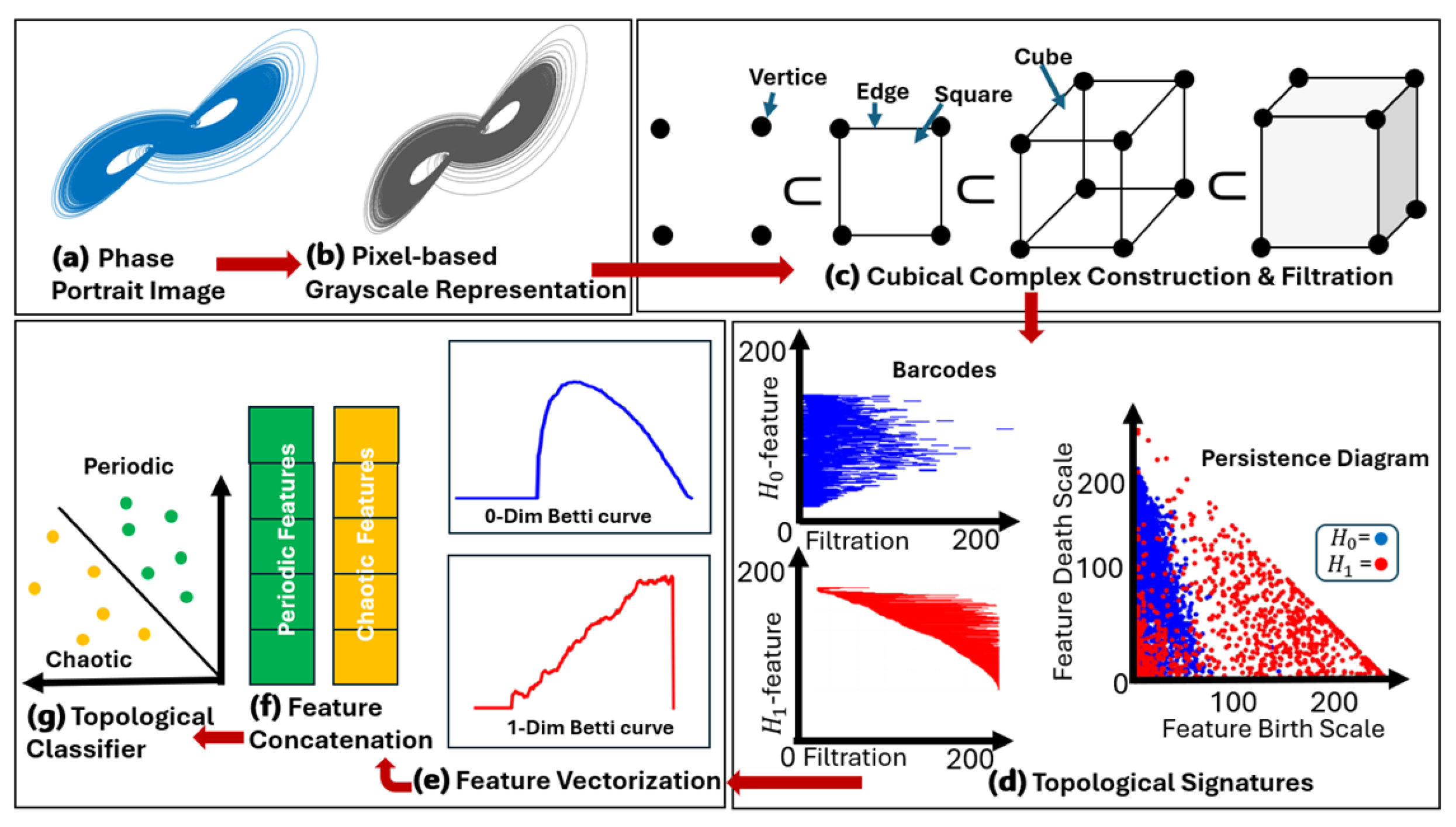
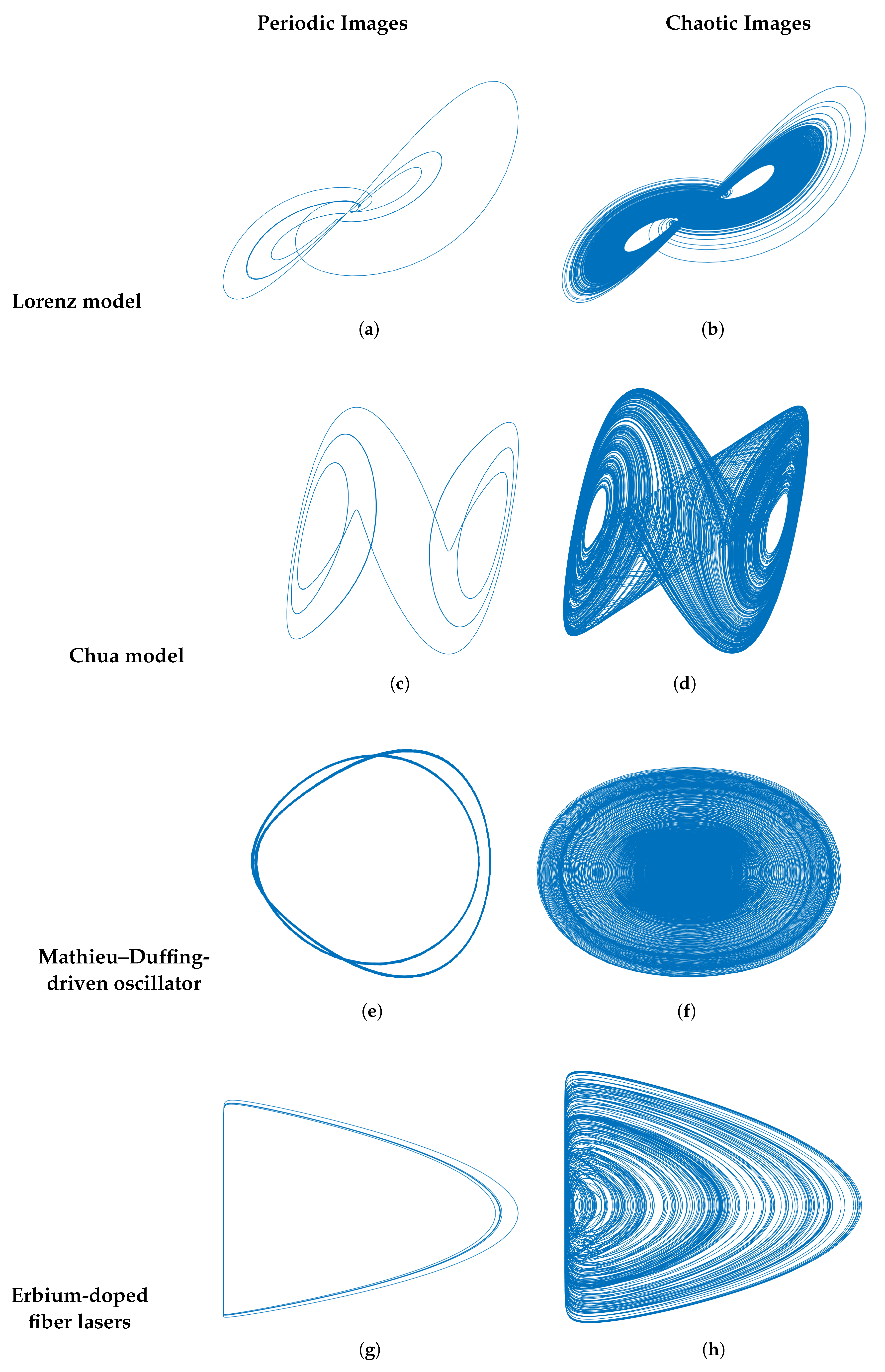
In the first stage, portrait datasets are generated from several nonlinear dynamical systems described in Section 2, including the Lorenz system, Chua’s circuit, MD-driven oscillator, and EDFL model. The original dataset image of the Lorenz model is shown in Figure 2a. For each system, the governing differential equations were numerically integrated over a range of parameter values to obtain PPs spanning both the periodic and chaotic regimes. The periodic and chaotic regimes considered in this study were selected via control-parameter analysis, based on the geometric bifurcation behavior and PP structures of each nonlinear dynamical system. These PPs served as the primary input data for subsequent analysis. The sample PPs corresponding to all the considered models are illustrated in Figure 1.

4.2. Preprocessing of Phase Portrait

The generated PPs data were passed through several preprocessing steps to standardize the dataset and prepare the images for topological analysis. First, each image was resized and cropped to remove unnecessary margins and ensure consistent spatial representation across the dataset. Next, we convert the image from $\left(RGB\right)$ color channels to grayscale and resize it to a fixed resolution of $512\times 512$ pixels. In this representation, the grayscale intensity values range from 0 to 255, where 0 corresponds to black and 255 corresponds to white. Figure 2b shows a grayscale image used for cubical filtration.

This preprocessing stage is essential for automated analysis because it provides uniformity in the dataset and enhances the reliability of subsequent topological computations. The resulting preprocessed images were then used as the input for the topological feature extraction stage.

4.3. Topological Feature Extraction

To analyze the structural properties of the PPs, we employed TDA techniques. In particular, topological features are extracted using CH, which is well-suited for grid-based data such as digital images. PPs are represented as grayscale images; each image naturally forms a cubical complex based on its underlying pixel grid. In the proposed framework, PPs images generated from the nonlinear trajectories are represented on a pixel grid, where each pixel corresponds to an elementary two-dimensional cube (square). The grayscale intensity values assigned to the pixels define the filtration process, such that pixels progressively enter the cubical complex as the threshold value increases. Consequently, the topological analysis is performed on the pixel-based image representation of the attractor rather than directly on the phase-space trajectories, while preserving the geometrical shape of the phase portraits.

The maximum threshold value is set to $N=255$, which corresponds to the highest intensity in the grayscale images. To compute the topological information of the images, we applied a pixel-based filtration, the V-construction [37]. This filtration assigns an intensity value to each pixel and progressively generates a sequence of cubical complexes as the filtration parameter increases. As the filtration parameter value increases, it tracks the evolution of topological features in the image, including connected components and holes. As depicted in Figure 2c, the filtration sequence illustrates the process used to compute CH.

Using this filtration process, CH was computed to track the evolution of topological structures across different threshold levels. For each image, PDs are obtained that record the births and deaths of topological features. In this study, we focus on the first two homology dimensions, $H_0$ and $H_1$, since the considered phase portrait representations are two-dimensional image-based structures, while higher-dimensional homology groups are less informative for the present framework.

• $H_0$ represents the connected components in the image.
• $H_1$ captures loop or hole structures present in the phase portraits.

Due to the use of CH-based topological descriptors, which are known to capture global geometric structures that are stable under small perturbations, the proposed framework is expected to exhibit a degree of robustness to moderate noise in phase portrait representations. As illustrated in Figure 2d, two types of topological representations are presented: PDs and barcodes. Barcodes and PDs are equivalent representations of PH, preserving the same birth–death structure of topological features, thus providing invariant summaries of the data under continuous transformations.

4.4. Topological Feature Vectorization

PDs contain different numbers of points, making them unsuitable for direct use in ML algorithms. Therefore, a vectorization step is required to convert these diagrams into a fixed-length feature representation. Several techniques have been proposed for converting PDs into fixed-length feature vectors. These include persistence images [38], persistence landscapes [39], persistent entropy [40], persistence Silhouettes [41], Betti curves [42], and persistence curves [43]. Among these approaches, Betti curves were selected in this study because they provide a compact and computationally efficient vectorization of PDs while preserving the essential topological evolution across the filtration process.

We employed the Betti curve representation to obtain a feature vector of uniform length. A Betti curve counts the number of active topological features at each filtration level, providing a compact summary of a persistence diagram. Let ‘d’ denote the dimension of the PH group, and let $D={\left\{(b_i,d_i)\right\}}_{i=1}^n$ represent the corresponding persistence diagram, where ‘$b_i$’ and ‘$d_i$’ indicate the birth and death times of the ith topological feature.

The Betti curve summarizes the number of topological features that remain at a given filtration value. Formally, it is defined through the function $B_d:\mathbb{R}\to \mathbb{N}$, which counts the number of persistence intervals that contain a filtration parameter $ϵ$ as defined in Equation (11).

$$B_d\left(ϵ\right)=\left|\left\{(b_i,d_i):ϵ\in [b_i,d_i]\right\}\right|.$$

(11)

In other words, $B_d\left(ϵ\right)$ measures the number of topological features present at the filtration level ‘$ϵ$’. The function $B_d$ plotted over ‘$ϵ$’ produces a curve known as the Betti curve.

For each persistence diagram obtained from the dataset, the corresponding Betti curve was computed and discretized into a fixed-length feature vector. In this study, each Betti curve is discretized into a feature vector $\mathbf{x}\in {\mathbb{R}}^{200}$, ensuring that all images are represented in a common feature space with a fixed dimension. As illustrated in Figure 2e, the resulting topological feature vectors corresponding to both $H_0$ and $H_1$ dimensions are derived from the PD. This unified representation enables the effective utilization of the extracted topological features as inputs for ML models.

4.5. Machine Learning Classification

After obtaining the fixed-length feature vectors from the Betti curves, we used these features to train supervised ML models for classification. We further concatenate the features of the same dimension from ($H_0$ and $H_1$) for both the periodic and chaotic classes to construct a unified binary feature vector. As shown in Figure 2f, the resulting representation illustrates the concatenated features of the two classes. The dataset was manually divided into two categories based on the dynamic behavior of the systems: periodic and chaotic PPs for each model. The extracted topological features were provided as inputs to several classification algorithms, including Support Vector Machines (SVMs), random forests, and extreme gradient boosting (XGBoost). These models are trained to distinguish between periodic and chaotic dynamics by learning patterns in the topological feature space. The topological ML classifier distinguishes between periodic and chaotic portraits, as shown in the Figure 2g.

The proposed pipeline is computationally efficient because CH is computed directly from pixel-based phase portrait images, avoiding costly point-cloud construction. Moreover, Betti-curve representations provide compact feature vectors, reducing computational overhead during classification. All experiments were performed on a standard workstation equipped with an Intel Core i7 (11th generation) processor and 128 GB RAM, demonstrating the feasibility and scalability of the proposed method.

The performance of the classifiers was evaluated using standard metrics, allowing us to assess the effectiveness of the proposed topological framework for classifying dynamical regimes.

5. Results and Discussion

5.1. Topological Signatures: Portraits to Betti Curves

For all the considered dynamical systems, phase portrait images were first generated and manually categorized into two classes: periodic and chaotic regimes. For each system, we constructed a dataset of 500 phase portraits to ensure a balanced representation of both behaviors. The dataset was then split into training and test sets at 80–20% to enable reliable evaluation of the classification models.

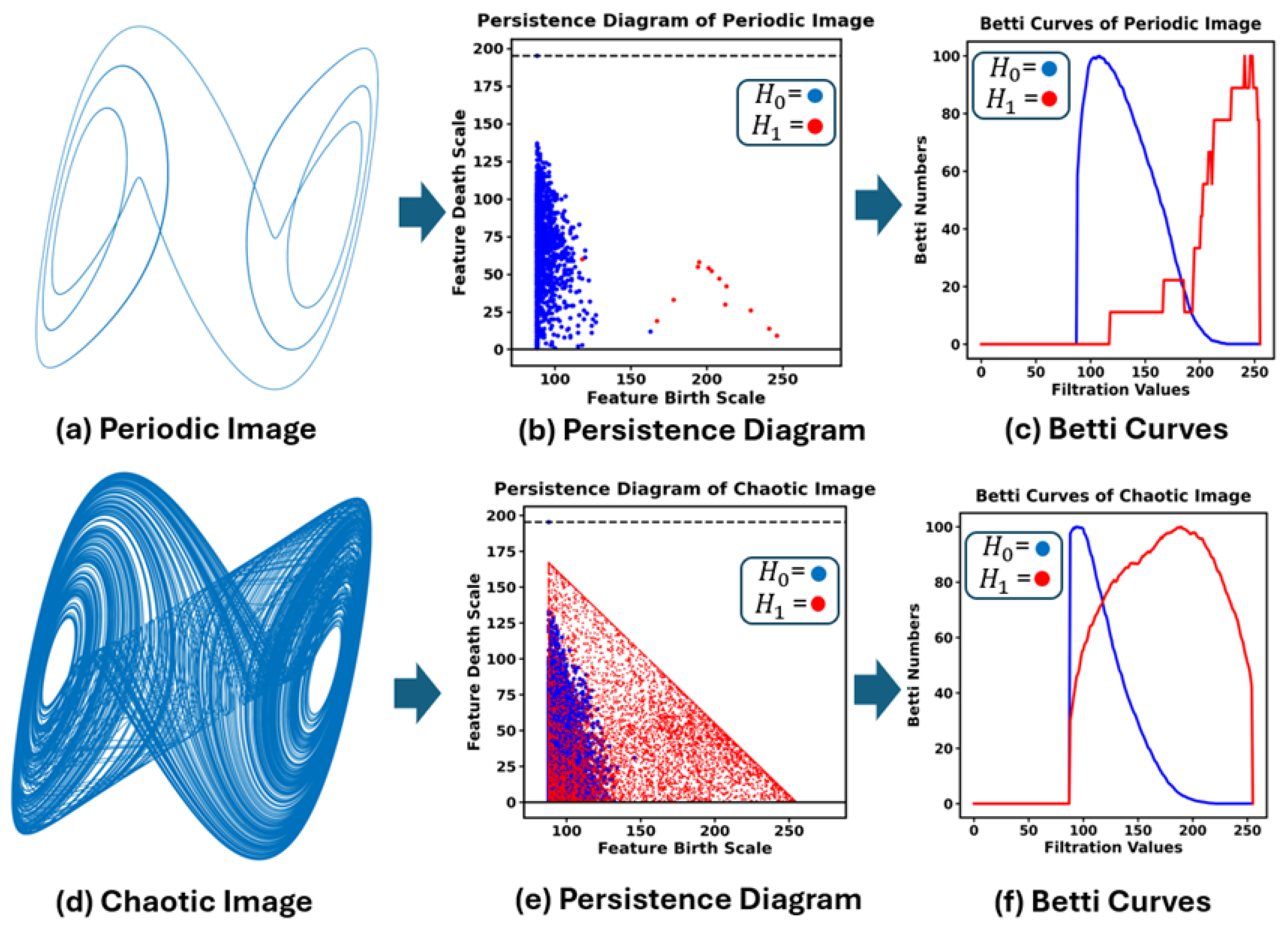
The first step in the proposed pipeline is the computation of PDs using CH applied to the PPs images. Figure 3 illustrates representative examples from the Lorenz system for both periodic (Figure 3a) and chaotic regimes (Figure 3d). As observed in the PDs, periodic attractors exhibit a relatively small number of topological features in both the $H_0$ and $H_1$ dimensions, reflecting their regular, structured geometry. In contrast, chaotic attractors exhibit a significantly larger number of persistent points, indicating a richer, more complex topological structure.

This observation was further supported by a quantitative analysis. For the periodic phase portrait of the Chua model, the total number of $H_0$ features was 1656, and the number of $H_1$ features was 13 (see Figure 3b). In contrast, for the chaotic regime, the number of $H_0$ features increases to 6931, whereas $H_1$ features rise significantly to 7221 in the corresponding PD in Figure 3e. This substantial increase in topological features clearly demonstrates the greater geometric complexity and richer loop structures in chaotic dynamics, underscoring the effectiveness of topological descriptors in distinguishing between dynamical regimes.

Furthermore, the Betti curves corresponding to $H_0$ and $H_1$ dimensions were computed from the PDs, as shown in Figure 3c,f. These curves provide a compact and informative representation of the evolution of topological features across the filtration scales. We systematically applied this pipeline to all PPs across all datasets, and the resulting Betti curves were used to construct the final feature vectors for ML classification.

5.2. Evaluation Metrics

In ML, the performance of the proposed metrics is used to set baselines for methods such as accuracy, precision, recall, and F1 scores. The confusion metrics for the classification have four outcomes. Using confusion metrics, we extracted additional metrics from the actual values. These metrics were used in the classification tasks to assess the model performance (

Table 3. Performance evaluation metrics based on confusion matrix.

Metric	Formula	Interpretation
Accuracy	${\displaystyle \frac{TP+TN}{TP+TN+FP+FN}}$	Overall performance of the model
Precision	${\displaystyle \frac{TP}{TP+FP}}$	How accurate the positive predictions are
Recall (Sensitivity)	${\displaystyle \frac{TP}{TP+FN}}$	Coverage of actual positive samples
Specificity	${\displaystyle \frac{TN}{TN+FP}}$	Coverage of actual negative samples
F1 Score	${\displaystyle \frac{2TP}{2TP+FP+FN}}$	Hybrid metric useful for unbalanced classes

).

Different supervised ML classifiers were applied to predict whether the data belong to the periodic or chaotic class. The possible outcomes were true positive (TP), false positive (FP), true negative (TN), and false negative (FN).

• TP (True Positive): When the prediction and the actual value are positive.
• TN (True Negative): When the prediction and the actual value are negative.
• FP (False Positive): When the prediction is positive but the actual value is negative.
• FN (False Negative): When the prediction is negative but the actual value is positive.

For benchmarking, we employed several classical ML algorithms, including Support Vector Machine (SVM), K-Nearest Neighbors (KNN), Random Forest (RF), Extreme Gradient Boosting (XGBoost), and Gaussian Naïve Bayes. The KNN algorithm is used for classification tasks by leveraging distance-based learning. In addition, Random Forest is an ensemble learning method that improves predictive performance by combining multiple decision trees. XGBoost was used for its efficiency and scalability in gradient boosting, whereas Gaussian Naïve Bayes was included as a probabilistic classifier under the assumption of feature independence.

5.3. Classification Results Under $H_0$ and $H_1$ for the Chua Model

We used the Chua system to present the experimental results and evaluate the performance of various ML techniques, including XGBoost, SVM, Gaussian Naïve Bayes, KNN, and RF. The performance of these models was assessed under two hypothesis, $H_0$ and $H_1$, using evaluation metrics such as accuracy, F1-score, precision, sensitivity, and specificity.

Under the hypothesis $H_0$ (0-dimensional feature representation), the results summarized in

Table 4. Performance under $H_0$ (0-dimensional feature representation) for Chua model.

Classifier	Accuracy (%)	F1-Score (%)	Precision (%)	Sensitivity (%)	Specificity (%)
XGBoost	98	98	100	97	100
SVM	97	97	97	97	98
Gaussian Naïve Bayes	91	89	83	97	87
KNN	97	97	97	97	98
Random Forest	98	98	100	97	100

show that XGBoost and RF exhibit strong performance, particularly in terms of precision and specificity, achieving perfect precision (100%) and high specificity. The SVM and KNN also demonstrated competitive, stable results across all metrics. In contrast, Gaussian Naïve Bayes shows comparatively lower performance, particularly in the F1-score and specificity, likely because its simplified probabilistic modeling is less effective in capturing the complex nonlinear patterns represented by the extracted topological features.

Under hypothesis $H_1$ (1-dimensional feature representation), the results presented in

Table 5. Performance under $H_1$ (1-dimensional feature representation) for Chua model.

Classifier	Accuracy $(\%)$	F1-Score (%)	Precision (%)	Sensitivity (%)	Specificity (%)
XGBoost	98	98	100	96	100
SVM	96	96	97	94	97
Gaussian Naïve Bayes	95	94	97	92	97
KNN	99	99	98	100	97
Random Forest	99	99	100	98	100

indicate an overall improvement in performance. In particular, KNN and RF achieved the highest accuracy and F1-score of 99%, whereas XGBoost maintained strong precision and specificity. Compared to $H_0$, the results under $H_1$ show a clear enhancement in the predictive capability. Specifically, the overall accuracy and F1-score improved to 99% indicating a better balance between precision and recall. This demonstrates the effectiveness of the proposed feature representation in improving the classification performance.

5.4. Classification Results Under $H_0$ and $H_1$ for the Lorenz Model

We used the Lorenz system to generate complex nonlinear patterns, which were then used for feature extraction and classification. The performance of different ML classifiers, as in the Chua model, is evaluated under two hypothesis, $H_0$ (0-dimensional features) and $H_1$ (1-dimensional features).

Under the hypothesis $H_0$, the overall performance of the classifiers was moderate, as summarized in

Table 6. Performance under $H_0$ (0-dimensional feature representation) for the Lorenz model.

Classifier	Accuracy (%)	F1-Score (%)	Precision (%)	Sensitivity (%)	Specificity (%)
XGBoost	93	93	95	90	95
SVM	80	81	78	84	75
Gaussian Naïve Bayes	86	86	89	82	89
KNN	93	93	92	94	91
Random Forest	93	93	92	94	91

. XGBoost, KNN, and RF achieved an accuracy of 93%. SVM shows a relatively lower accuracy of 80%. Gaussian Naïve Bayes demonstrated comparatively lower performance, with an accuracy of 86%, reflecting its limitations in capturing the data’s underlying nonlinear structure.

In contrast, under hypothesis $H_1$, the results presented in

Table 7. Performance under $H_1$ (1-dimensional feature representation) for the Lorenz model.

Classifier	Accuracy (%)	F1-Score (%)	Precision (%)	Sensitivity (%)	Specificity (%)
XGBoost	98	98	98	97	98
SVM	98	98	100	97	100
Gaussian Naïve Bayes	98	98	100	97	100
KNN	98	98	100	97	100
Random Forest	98	98	100	97	100

show a significant improvement across all classifiers. All models achieved accuracies and F1-Scores of 98%, demonstrating consistent, robust classification performance. Notably, the precision and specificity reached 100% for most classifiers, whereas the sensitivity improved to 97%, indicating a balanced and reliable prediction capability. In particular, Gaussian Naïve Bayes showed a remarkable improvement, with the accuracy increasing from 86% in $H_0$ to 98% in $H_1$. 1-dimensional feature representation highlights the effectiveness in capturing the intrinsic dynamics of the Lorenz system and in enhancing classification performance.

5.5. Classification Results Under $H_0$ and $H_1$ for the Erbium-Doped Fiber Laser Model

The Erbium-doped fiber laser model was analyzed using the same ML classifiers. The performance was evaluated under two hypothesis, $H_0$ and $H_1$, using standard metrics such as accuracy, F1-score, precision, sensitivity, and specificity.

Under the hypothesis $H_0$, the classifiers demonstrated stable and competitive performance, as summarized in

Table 8. Performance under $H_0$ (0-dimensional feature representation) for the laser model.

Classifier	Accuracy (%)	F1-Score (%)	Precision (%)	Sensitivity (%)	Specificity (%)
XGBoost	93	93	91	95	92
SVM	95	95	95	95	96
Gaussian Naïve Bayes	93	93	91	95	92
KNN	95	95	95	95	96
Random Forest	93	93	91	95	92

. SVM and KNN achieved the highest accuracy and F1-score (95%), along with balanced sensitivity and specificity. XGBoost, Gaussian Naïve Bayes, and RF showed slightly lower but consistent results, with an accuracy of approximately 93%. Overall, the models exhibited a well-balanced classification behavior under the 0-dimensional feature setting.

In contrast, under hypothesis $H_1$, the results presented in

Table 9. Performance under $H_1$ (1-dimensional feature representation) for the laser model.

Classifier	Accuracy (%)	F1-Score (%)	Precision (%)	Sensitivity (%)	Specificity (%)
XGBoost	93	94	96	93	95
SVM	95	96	96	95	95
Gaussian Naïve Bayes	81	81	100	68	100
KNN	93	94	93	96	90
Random Forest	91	93	93	93	90

indicate that the performance varies across classifiers. SVM maintained strong, consistent results, with an improved F1-score (96%) and high precision (96%). XGBoost also shows improved precision and specificity compared to $H_0$. However, Gaussian Naïve Bayes exhibited a significant drop in performance, with accuracy and F1-score decreasing to 81% and sensitivity reducing to 68%, despite achieving perfect precision and specificity. KNN maintained a balanced performance with improved sensitivity (96%), whereas RF showed a slight decrease in overall accuracy. These results indicate that, unlike previous systems, the 1-dimensional feature representation does not uniformly improve the performance of all classifiers in the laser model, highlighting the sensitivity of certain models to feature representation.

5.6. Classification Results Under $H_0$ and $H_1$ for the Mathieu–Duffing-Driven Oscillator

The MD-driven oscillator is a well-known nonlinear dynamical system used to describe complex oscillatory and chaotic behaviors. In this study, multiple ML classifiers, including XGBoost, SVM, Gaussian Naïve Bayes, KNN, and RF, were applied to evaluate classification performance under two hypothesis, $H_0$ and $H_1$, using dimensional features.

Under the hypothesis $H_0$, most classifiers already demonstrated strong performance, as summarized in

Table 10. Performance under $H_0$ (0-dimensional feature representation) for the Mathieu–Duffing-driven oscillator.

Classifier	Accuracy (%)	F1-Score (%)	Precision (%)	Sensitivity (%)	Specificity (%)
XGBoost	98	98	98	98	98
SVM	99	99	100	98	100
Gaussian Naïve Bayes	86	86	91	81	91
KNN	97	97	100	95	100
Random Forest	99	99	98	100	98

. SVM and RF achieved high accuracy (99%) with excellent precision and specificity. XGBoost and KNN also achieved competitive results, with accuracies above 97%. However, Gaussian Naïve Bayes performed comparatively worse, with an accuracy of 86%, indicating its limited ability to capture the underlying nonlinear dynamics in the 0-dimensional feature space.

In contrast, under hypothesis $H_1$, the results presented in

Table 11. Performance under $H_1$ (1-dimensional feature representation) for the Mathieu–Duffing-driven oscillator.

Classifier	Accuracy (%)	F1-Score (%)	Precision (%)	Sensitivity (%)	Specificity (%)
XGBoost	100	100	100	100	100
SVM	100	100	100	100	100
Gaussian Naïve Bayes	98	98	98	100	97
KNN	100	100	100	100	100
Random Forest	100	100	100	100	100

show a significant improvement across all classifiers. XGBoost, SVM, KNN, and RF achieved perfect classification performance, achieving 100% accuracy, F1-score, precision, sensitivity, and specificity. Gaussian Naïve Bayes also showed a substantial improvement, with accuracy increasing from 86% to 98% and sensitivity reaching 100%. Overall, the results clearly indicate that the 1-dimensional feature representation significantly enhances the classification performance. In particular, the accuracy improves from approximately 97% under $H_0$ to 100% under $H_1$, demonstrating the effectiveness of the proposed feature-extraction approach in capturing the complex dynamics of the MD-driven system. To further evaluate the robustness of the obtained results and reduce the possibility of overfitting, an additional 5-fold cross-validation experiment was conducted, demonstrating consistently stable classification performance across different data partitions.

5.7. Cross-Validation Analysis

To evaluate the reproducibility and statistical reliability of the proposed framework, additional stratified five-fold cross-validation experiments were conducted using the best-performing $H_1$ feature representation. Since the $H_1$ features consistently achieved superior classification performance across all nonlinear systems, the analysis was performed using the two best-performing classifiers, namely XGBoost and Random Forest. The mean and standard deviation of the evaluation metrics obtained across the five folds are summarized in

Table 12. Five-fold cross-validation performance using $H_1$ features for all systems.

Dataset	Classifier	Accuracy (%)	F1-Score (%)	Precision (%)	Recall (%)
Chua	XGBoost	$97.18\pm 1.35$	$97.63\pm 1.31$	$96.88\pm 1.98$	$96.79\pm 1.79$
Chua	Random Forest	$97.78\pm 1.51$	$97.12\pm 2.01$	$97.34\pm 1.35$	$98.27\pm 1.11$
Lorenz	XGBoost	$97.80\pm 0.75$	$98.01\pm 0.68$	$98.58\pm 1.32$	$97.49\pm 1.82$
Lorenz	Random Forest	$98.40\pm 0.49$	$98.64\pm 0.44$	$98.56\pm 1.32$	$98.77\pm 1.33$
Mathieu–Duffing	XGBoost	$99.76\pm 0.48$	$99.77\pm 0.46$	$99.55\pm 0.91$	$100.00\pm 0.00$
Mathieu–Duffing	Random Forest	$100.00\pm 0.00$	$100.00\pm 0.00$	$100.00\pm 0.00$	$100.00\pm 0.00$
Laser	XGBoost	$92.58\pm 1.17$	$92.56\pm 2.10$	$91.61\pm 1.85$	$93.66\pm 2.68$
Laser	Random Forest	$92.60\pm 2.29$	$92.52\pm 1.41$	$91.76\pm 1.44$	$94.49\pm 1.38$

.

The obtained results demonstrate low variability across folds for all considered systems, indicating the robustness and stability of the proposed framework under different data partitions. In particular, the Mathieu–Duffing system achieved near-perfect classification performance with extremely small standard deviations, whereas the Lorenz system also exhibited highly stable behavior. Although slightly larger variations were observed for the Chua and laser systems, the overall results confirm the reproducibility and strong generalization capability of the extracted topological features.

5.8. Classification Results Using Combined Features ($H_0+H_1$)

To further evaluate the effectiveness of the proposed topological machine learning pipeline, we combined 0- and 1-dimensional features ($H_0+H_1$) and analyzed their impact on classification performance across different dynamical systems. The results for each system are summarized in

Table 13. Performance using combined features ($H_0+H_1$) for the Chua model.

Classifier	Accuracy (%)	F1-Score (%)	Precision (%)	Sensitivity (%)	Specificity (%)
XGBoost	97	98	100	97	100
SVM	96	96	97	95	98
Gaussian Naïve Bayes	94	93	90	95	98
KNN	98	98	97	98	98
Random Forest	98	98	100	97	100

,

Table 14. Performance using combined features ($H_0+H_1$) for the Lorenz model.

Classifier	Accuracy (%)	F1-Score (%)	Precision (%)	Sensitivity (%)	Specificity (%)
XGBoost	95	95	96	93	97
SVM	90	89	95	84	96
Gaussian Naïve Bayes	60	63	57	70	50
KNN	94	94	97	90	98
Random Forest	96	95	97	93	98

,

Table 15. Performance using combined features ($H_0+H_1$) for the laser model.

Classifier	Accuracy (%)	F1-Score (%)	Precision (%)	Sensitivity (%)	Specificity (%)
XGBoost	96	96	97	95	98
SVM	95	95	97	93	98
Gaussian Naïve Bayes	82	77	90	68	94
KNN	96	96	97	95	98
Random Forest	96	96	95	97	96

and

Table 16. Performance using combined features ($H_0+H_1$) for the Mathieu–Duffing model.

Classifier	Accuracy (%)	F1-Score (%)	Precision (%)	Sensitivity (%)	Specificity (%)
XGBoost	97	97	97	97	97
SVM	98	98	97	100	97
Gaussian Naïve Bayes	92	92	94	91	93
KNN	98	98	97	100	97
Random Forest	98	98	97	95	97

.

For the Chua system, as reported in Table 13, the combined feature representation achieved a high classification performance across all models. In particular, KNN and RF achieved the highest accuracy of 98%, while XGBoost and SVM also demonstrated strong, stable results. Compared with individual feature representations, the combined features provide a balanced improvement while maintaining high precision and specificity.

For the Lorenz system, the results presented in Table 14 show that the combined features achieved an accuracy of 96% for most classifiers. Although this is slightly lower than the performance obtained using $H_1$ alone, it still outperforms the $H_0$ representation. This indicates that the 1-dimensional features already capture most of the discriminative information, whereas the combined representation offers a more robust alternative.

In the case of the EDFL model, as illustrated in Table 15, the combined features provided competitive performance. RF achieved the highest accuracy of 96%, whereas XGBoost and KNN maintained stable results. However, Gaussian Naïve Bayes exhibited a significant drop in performance, indicating that certain classifiers remained sensitive to feature fusion.

For the MD-driven oscillator, the results summarized in Table 16 indicate a strong performance across all classifiers, with SVM, KNN, and RF achieving up to 98% accuracy. Although the performance is slightly lower than the perfect results obtained using $H_1$, the combined representation still maintains a high accuracy and robustness.

Overall, the combined feature representation ($H_0+H_1$) demonstrated competitive, stable performance across all systems. While $H_1$ generally provides the highest accuracy, the combined features offer a balanced trade-off between robustness and predictive performance. These findings confirm that multidimensional topological features capture complementary information, enhancing the classification of PPs in nonlinear dynamical systems.

5.9. Confusion Matrix Analysis

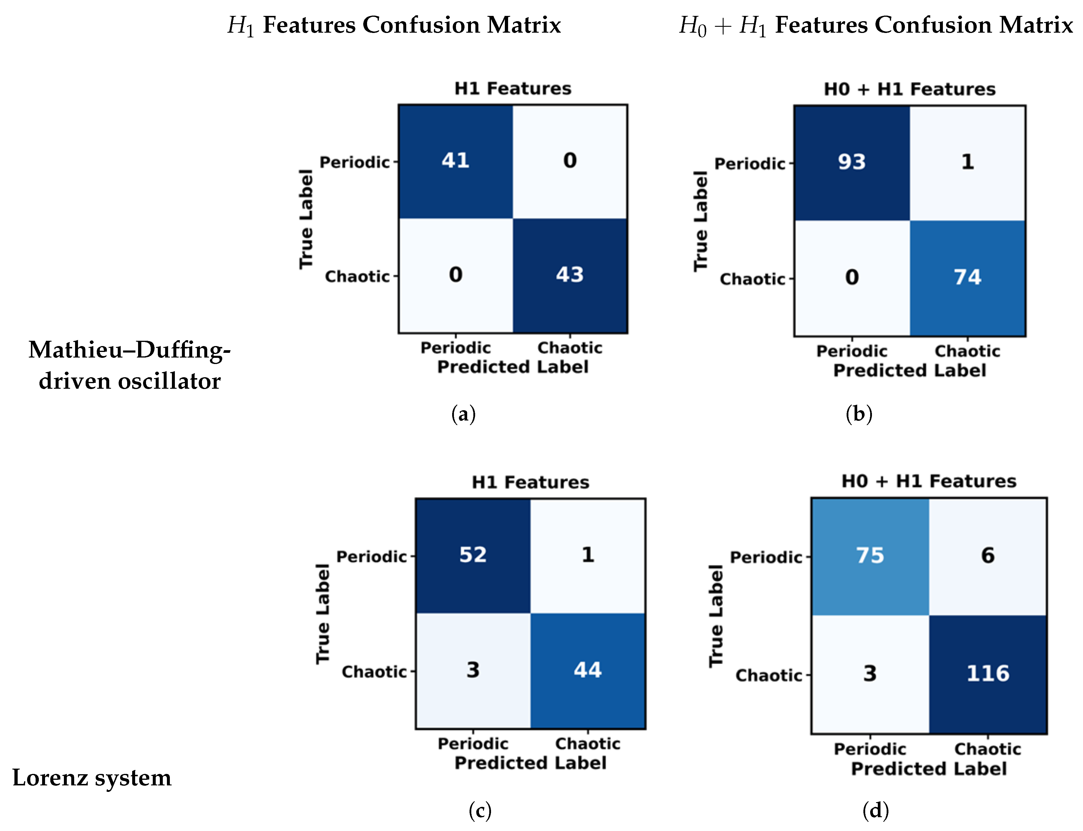
To further investigate the classification performance of the proposed topological ML pipeline, confusion matrix analysis was performed using the XGBoost classifier for both the Mathieu–Duffing and Lorenz systems. The confusion matrices provide a detailed evaluation of the classification outcomes by explicitly showing the number of correctly and incorrectly classified samples for the periodic and chaotic regimes. Figure 4 presents a combined visualization consisting of four panels corresponding to the different feature representations and dynamical systems.

In Figure 4, Panel (a) illustrates the confusion matrix for the MD-driven system using $H_1$ features. The model achieved perfect classification performance, correctly classifying all periodic and chaotic samples with no misclassifications. This indicates that the 1-dimensional topological features are highly effective in capturing the intrinsic structure of the MD-driven system.

Panel (b) shows the confusion matrix for the MD-driven system using the combined feature representation ($H_0+H_1$). In this case, the model maintained near-perfect performance, with only a single misclassification, a false positive. The high numbers of true positives and true negatives demonstrate that the combined features preserve the discriminative power of $H_1$ while introducing only slight redundancy, resulting in minimal classification error.

For the Lorenz system, Panel (c) presents a confusion matrix using $H_1$ features. The results indicate a strong classification performance, with the majority of the samples correctly classified. However, a small number of misclassifications, including both false positives and false negatives, were observed, suggesting that the Lorenz system exhibits more complex dynamics that are slightly more difficult to separate than those of the MD-driven system.

Panel (d) illustrates the confusion matrix for the Lorenz system using the combined feature representation ($H_0+H_1$). In this case, the number of correctly classified chaotic samples (true positives) increased significantly, indicating improved sensitivity toward chaotic behavior. However, this improvement was accompanied by a slight increase in false positives, reflecting a trade-off between sensitivity and specificity. This behavior suggests that the combined features enhance the detection of complex dynamical patterns while introducing a small degree of overclassification.

Overall, the confusion matrix analysis revealed that the $H_1$ feature representation provided highly accurate classification performance, particularly for the MD-driven system. The combined feature representation ($H_0+H_1$), on the other hand, offers more robust, balanced performance, especially for systems with more complex dynamics, such as the Lorenz model. These results confirm that multidimensional topological features effectively capture the underlying structure of nonlinear dynamical systems and significantly improve the classification of PPs.

5.10. t-SNE Visualization and Feature Space Analysis

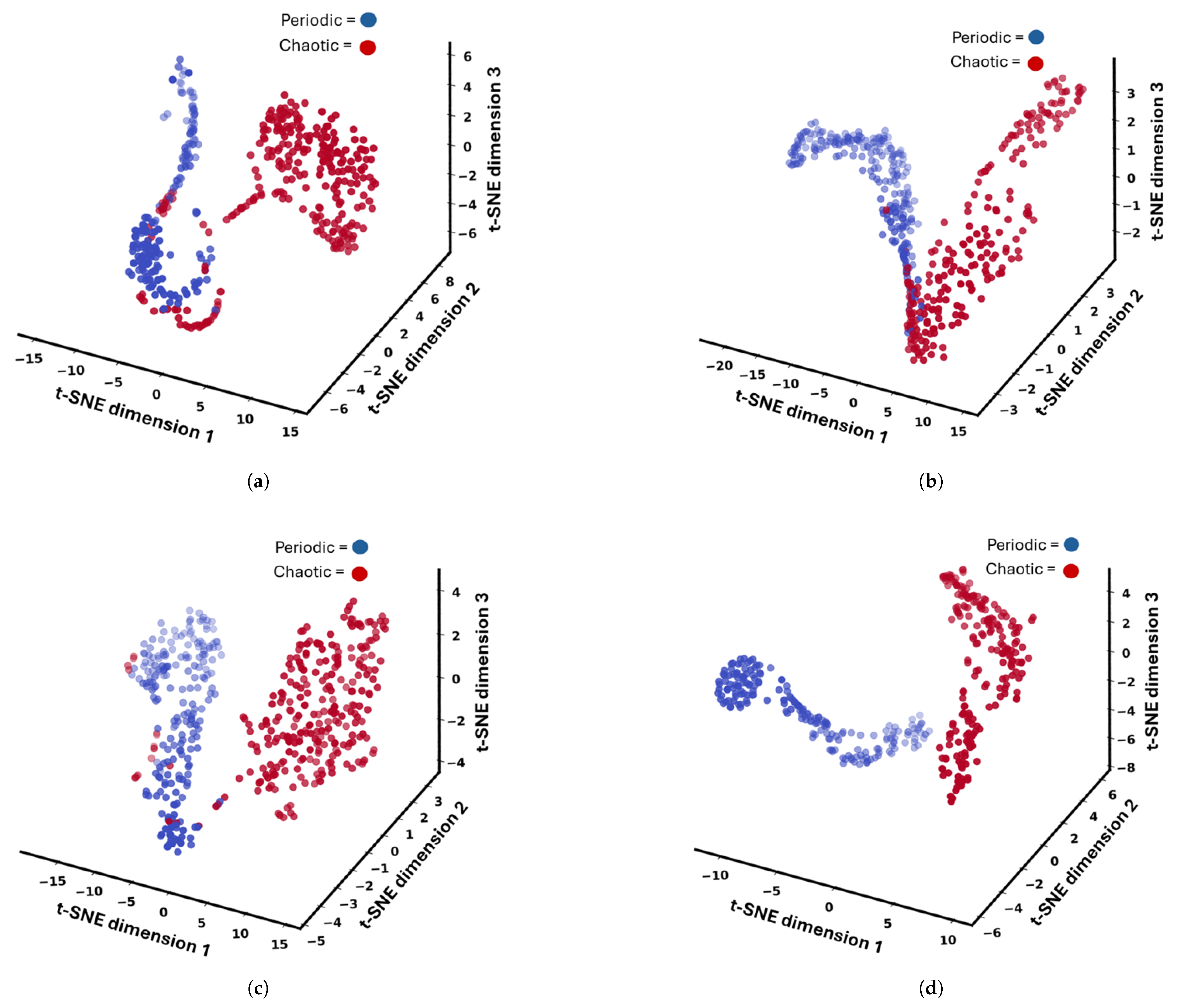
To further investigate the effectiveness of the extracted CH-based features, t-distributed Stochastic Neighbor Embedding (t-SNE) was employed to project the high-dimensional feature vectors into a three-dimensional space. This visualization enables an intuitive understanding of how well the proposed features discriminate between periodic and chaotic dynamics in different nonlinear systems.

Figure 5 presents the t-SNE embeddings of the four representative dynamical systems. In all the subfigures, the blue points correspond to periodic behavior, whereas the red points represent chaotic dynamics. A general observation across all cases is the formation of distinct clusters, indicating that the extracted topological features successfully encode the underlying dynamic differences.

For the Chua system, as shown in Figure 5a, a clear separation between the periodic and chaotic classes is observed. The periodic data form a relatively compact and structured cluster, whereas the chaotic data are more scattered and occupy a separate region of the embedding space. The cluster geometry was slightly curved, suggesting the presence of nonlinear relationships within the feature space. A few points near the boundary indicate possible transitional dynamics or bifurcation regions, which are typical of nonlinear circuit systems.

In the case of the EDFL, illustrated in Figure 5b, the separation between the two classes remains visible; however, a noticeable overlapping region is present. This overlap suggests that the transition from periodic to chaotic behavior in the laser system is gradual and complex. The t-SNE embedding also reveals a trajectory-like structure, indicating that the feature space preserves the system’s dynamics. This behavior highlights the sensitivity of the proposed features to subtle changes in the underlying system.

For the Lorenz system, as depicted in Figure 5c, the separation between periodic and chaotic dynamics is particularly distinct. The periodic cluster was compact and well-defined, whereas the chaotic cluster was more dispersed but clearly isolated. The minimal overlap between the two groups indicates high inter-class separability and low intra-class variance, demonstrating that the extracted features were highly effective for this system.

Similarly, the MD-driven oscillator shown in Figure 5d exhibits a well-defined and clean separation between the periodic and chaotic regimes. The periodic points formed a smooth and continuous structure, whereas the chaotic points were more elongated and scattered. The clear gap between the clusters further confirms the strong discriminative capability of feature representation for this system.

A consistent pattern was observed in the data distribution across all four systems. Periodic dynamics tend to form compact and smooth clusters, reflecting their regularity and stability. In contrast, chaotic dynamics are characterized by dispersed, irregular clusters that capture the inherent complexity and sensitivity of these systems.

Moreover, the presence of a small number of outliers or boundary points in each subfigure suggests regions of transitional behavior, bifurcations, or minor noise in the feature extraction process. These points pose challenging classification cases and provide additional insights into the robustness of the proposed approach.

Overall, the t-SNE visualizations in Figure 5a–d demonstrate that the CH-based features yield a well-structured and discriminative feature space. The clear separation between the periodic and chaotic regimes across different dynamical systems highlights the generality and effectiveness of the proposed topological framework.

6. Conclusions

In this study, a topological machine learning framework was developed for classifying dynamical regimes in nonlinear systems using phase portrait representations. The experimental results demonstrated highly accurate classification performance across multiple benchmark systems, with several models achieving near-perfect accuracy, particularly under the $H_1$ and combined-feature representations. In addition, the t-SNE visualizations revealed a well-structured feature space in which periodic and chaotic regimes were clearly separable, confirming the discriminative capability of the extracted topological features.

The results further revealed that the $H_1$ features play a crucial role in capturing loop structures and cyclic behavior, which are important signatures of chaotic dynamics. Moreover, combining $H_0$ and $H_1$ enhanced the robustness of the classification models, particularly for complex systems such as the Lorenz model, where feature fusion improved sensitivity to intricate dynamical patterns. The consistently strong performance across the Chua, Lorenz, MD-driven, and laser systems demonstrates the adaptability and effectiveness of the proposed pipeline for different classes of nonlinear dynamical systems, despite variations in system complexity and attractor structures.

Overall, the findings indicate that topological descriptors extracted from phase portraits provide an effective and interpretable representation of nonlinear dynamics. The ability of TDA to capture global geometric structures and preserve meaningful topological information makes it well-suited for analyzing complex dynamical behaviors. In addition to achieving strong classification performance, the proposed framework strengthens the connection between data-driven approaches and nonlinear dynamical system analysis. Future research will aim to extend this framework to higher-dimensional systems, integrate it with deep-learning architectures, assess its potential for detecting bifurcations and early transitions to chaos, examine its applicability to experimentally measured and real-world nonlinear systems using phase-space reconstruction and topological analysis of reconstructed attractor images, and evaluate its ability to distinguish between closely related and visually similar attractor structures.