Article

Research on Spatial Visual Servoing Control Algorithm Based on Orthogonal Visual System

1
AVIC Research Institute for Special Structures of Aeronautical Composites, Jinan 250023, China
2
AVIC Chengdu Aircraft Industrial (Group) Co., Ltd., Chengdu 610092, China
3
State Key Laboratory of Intelligent Manufacturing Equipment and Technology, Huazhong University of Science and Technology, Wuhan 430074, China
*
Author to whom correspondence should be addressed.
Mathematics 2026, 14(12), 2044; https://doi.org/10.3390/math14122044
Submission received: 26 April 2026 / Revised: 26 May 2026 / Accepted: 3 June 2026 / Published: 8 June 2026

Abstract

Robot control based on visual information perception has been a hot topic in the field of industrial robots, and the use of visual servoing technology to guide robots for high-precision spatial localization of machined workpieces has a wide range of application value. Aiming at the camera hand–eye calibration error and robot repositioning error, which have a large impact on the spatial localization and navigation accuracy, and when the binocular camera Z-direction accuracy is not high enough and the viewing angle is limited, etc., we propose a spatial visual servoing algorithm based on an orthogonal vision system that combines an eye-in-hand camera and an eye-to-hand camera in a hybrid configuration. By extracting sub-pixel image features in real time and deriving directionally decoupled interaction matrices, a linear controller is designed to guide the robot in the XY-plane and Z-direction separately. This decoupling strategy enlarges the convergence domain, avoids local minima caused by coupled degrees of freedom, and enhances system stability. To this end, the intrinsic calibration and hand–eye calibration of two cameras placed orthogonally are carried out firstly, and the accuracy of hand–eye calibration is not too demanding; then the sub-pixel level image position of the target is extracted in real time and the interaction matrix is derived and a linear controller is designed to control the robot’s motion; finally, the experiments of spatial localization accuracy are completed on the KUKA iiwa to validate the effectiveness of the method.

1. Introduction

With the continuous development of the manufacturing industry, the demand for high-precision robotic machining has been increasing. Not only has the quantity of machining tasks grown rapidly, but the quality requirements for these tasks have also become more stringent. In recent years, visual servoing systems have become a key solution for achieving high-precision spatial positioning and manipulation among various robotic control technologies, which have the advantages of more flexibility, high efficiency and robustness to operate in distinctive environments. However, there are various problems when applying visual servoing such as local minima, singularity, and visibility of feature points. These problems can be solved by using different features or using different camera placement schemes, which have drawn increasing attention and been a popular research field over the years.
It can be found that plenty of studies have been conducted on visual servoing to enable robots to perform various high-precision tasks. Visual servoing is a non-linear and strongly-coupled complex system, which involves the research fields of image processing, robot kinematics and dynamics, control theory, and so on [1]. In visual servoing, the control task involves manipulating a robot’s movements based on visual features extracted from real-time images of objects of interest [2,3]. The error function in visual servoing represents the difference between the current and desired positions of the robot or camera, with the goal of minimizing this error to zero. One or more cameras can be used to capture visual information for the robot’s control tasks [4,5,6].
There are two main control schemes commonly used in visual servoing: position-based visual servoing (PBVS) [7] and image-based visual servoing (IBVS) [8]. Their main difference lies in the computational space of the control inputs and the way visual information is processed. In the PBVS system, the control inputs are computed in 3D space, and the robot motion is controlled by estimating the position of image features in 3D space. Therefore, PBVS requires high calibration accuracy and is susceptible to calibration errors and environmental changes [9]. In the IBVS system, the control inputs are computed directly in the 2D image space, and the robot is controlled by adjusting the target position in the image. The main advantage of IBVS is the high robustness to camera and robot calibration errors, which makes it work well even when the calibration is not completely accurate, and it is particularly suitable for dynamic and complex environments. In addition, IBVS does not depend on the 3D target position, is computationally simplified, has high real-time performance, and is able to quickly adjust the robot’s movements through image feedback [10]. Therefore, we choose the IBVS method for localization.
IBVS operates by comparing real-time image data with a predefined reference signal, using the resulting image error as feedback to form a closed-loop control system. However, when designing the visual servoing controller, challenges arise, such as the singularity of the interaction matrix and the issue of local minima. When the initial and desired positions of the robot are significantly different, Y. Mezouar et al. [11] introduced a method that integrates path planning with image-based control. Youxin Li [12] proposed a planar visual servoing control approach that leverages direct image feedback combined with an artificial immune algorithm. This method is versatile, as it allows robot vision feedback control based on image features without the need for feature labeling or extraction. Vidyasager [13] proposed an image direct feedback method, where image pre-processing is followed by directly using the matching error between the target and the feedback image to guide the robot (camera) movement, eliminating the need for feature labeling and extraction. Lin Jia et al. [14] developed an image-based visual servoing method using a binocular camera for mobile robots, enabling autonomous navigation based on visual feedback. Huiguang Li et al. [15] proposed an adaptive visual servoing robot controller by constructing a Jacobian ratio matrix using image moments. Stability analysis demonstrated that this control system can effectively manage object motion in the image coordinate system, and experiments showed that the robot could achieve high-precision translation and rotation. For the SCMO-type soccer robot visual servoing system, Yiwei Feng et al. [16] applied image-based visual servoing and introduced a simple Kalman filter algorithm to improve robot positioning, tracking, and other tasks. Zhidan Dong et al. [17] presented a method that combines image invariant moments and the vector product approach to achieve six-DOF visual servoing control. Recent research has extended visual servoing into multi-camera calibration-less systems [18], diffusion-driven goal generation for wide-area tasks [19], uncalibrated adaptive control with dual-camera fusion [20,21], and robust adaptive learning strategies under uncertainties [22,23]. These works have improved adaptability and robustness, but they often rely on complex learning architectures or lack explicit spatial decoupling, which can limit precision in high-accuracy positioning tasks.
Visual servoing systems can be divided into two types based on the camera’s position: eye-in-hand and eye-to-hand. In the eye-in-hand system, the camera is mounted on the robot’s wrist. The camera directly observes the target object, and the field of view will be dynamically adjusted with the motion of the robot end, which helps to achieve higher spatial localization accuracy, but it is unable to directly observe the relative position between the robot end tool and the target, and it is more sensitive to the robot kinematics model and hand–eye calibration accuracy. In the eye-to-hand system, the camera is fixed in the robot’s workspace, observing both the target and the end-effector. The camera is able to cover a large workspace and is suitable for tasks such as multi-robot collaboration and machining of complex workpieces. Simultaneous observation of the target and the robot’s end contributes to better path planning and dynamic obstacle avoidance, and is not affected by the accuracy of hand–eye calibration, but the accuracy of the target is limited by the camera’s resolution and observation distance [24]. In our approach, we combine the advantages of both systems by using an orthogonal camera configuration. The XY-plane precision is ensured by the eye-in-hand system, where the camera is mounted on the robot’s wrist, while the Z-axis precision is controlled by a fixed camera located outside the robot, observing the target and the robot’s end-effector simultaneously. This setup allows for both high-precision control and a larger workspace, addressing the limitations of each individual system.
Motivated by the aforementioned studies, in this paper, we propose a spatial visual servoing system that integrates an eye-in-hand camera and an eye-to-hand camera in an approximately orthogonal arrangement. Unlike existing hybrid eye-in-hand/eye-to-hand visual servoing frameworks that often rely on heuristic switching between two camera views without explicit decoupling, our method derives directionally decoupled interaction matrices from the orthogonal configuration, which naturally separates XY-plane and Z-axis motions. This hybrid configuration naturally decouples the spatial control problem: the eye-in-hand camera governs the XY-plane motion, while the eye-to-hand camera independently regulates the Z-axis motion. Based on this setup, we derive simplified, direction-specific interaction matrices and design a staged control policy—first converging in XY, then moving in all three directions—which significantly enlarges the convergence domain, avoids local minima induced by fully coupled controllers, and guarantees stable convergence even from large initial offsets. The intrinsic and hand–eye calibrations are performed with only moderate accuracy requirements, and real-time sub-pixel corner features from chessboard targets drive the linear controller. Experiments on a KUKA iiwa robot (KUKA AG, Augsburg, Germany) confirm that the method achieves high-precision spatial localization while remaining robust to calibration errors. The following sections detail the calibration procedures, the derivation of the decoupled interaction matrices, and the experimental validation.

2. Preliminaries

2.1. Camera Image Processing

In the field of robotic vision, high-precision spatial positioning and manipulation require accurate camera calibration and image processing techniques. A critical step in achieving this is camera-intrinsic calibration, including the focal length, optical center, and lens distortion coefficients. These intrinsics are essential for transforming 2D image coordinates into 3D world coordinates, enabling the robot to accurately interpret visual information for tasks such as navigation and manipulation.
The intrinsics of a camera can be represented by the camera matrix K :
K = f x 0 c x 0 f y c y 0 0 1
where f x and f y are the focal lengths in terms of pixels (usually f x = f M x M , with f being the focal length in physical units, M x and M representing pixel size and resolution), and ( c x , c y ) is the optical center coordinate in the image plane. The camera calibration process involves capturing multiple images of a chessboard from various angles. The known geometry of the chessboard pattern allows us to establish correspondences between 3D world coordinates and 2D image coordinates. Using these correspondences, the camera intrinsics can be estimated.
Cameras suffer from lens distortion, which causes straight lines to appear curved in captured images. This distortion is typically modeled by the radial distortion parameters k 1 , k 2 , k 3 and tangential distortion parameters p 1 , p 2 . The distortion model is given by:
x d = x ( 1 + k 1 r 2 + k 2 r 4 + k 3 r 6 ) + 2 p 1 x y + p 2 ( r 2 + 2 x 2 ) y d = y ( 1 + k 1 r 2 + k 2 r 4 + k 3 r 6 ) + 2 p 1 ( r 2 + 2 y 2 ) + p 2 x y
where ( x d , y d ) are the distorted coordinates, ( x , y ) is the undistorted coordinate, and r = x 2 + y 2 is the radial distance from the center of the image.
To correct for this distortion, the inverse distortion function is applied to the image, resulting in an undistorted image where straight lines appear correctly. The camera matrix K and the distortion coefficients are computed during the calibration process using methods such as Zhang’s method [25], which minimizes the reprojection error between the projected and actual points.
In order to be able to accomplish accurate spatial localization, we choose a standard chessboard as the target. The image is corrected using the intrinsics obtained from the calibration, and by calculating the gradient information of each pixel in the image, the Harris corner detector is able to find the corner points in the image, which are then extracted at the sub-pixel level using Gaussian-weighted least squares.

2.2. Hand–Eye Calibration

To transform the camera coordinate system into the robot coordinate system, hand–eye calibration is required. Depending on the relative position of the camera and the robot, there are two modes: “eye-in-hand” and “eye-to-hand” (see Figure 1).
A. Eye-in-hand: The camera is mounted at the robot’s end, and the calibration chessboard is fixed on the experimental platform. When the robot moves, the relationship between the robot base frame and the chessboard frame remains constant. Using images of the chessboard taken by the camera, we compute the transformation from the camera frame to the chessboard frame. Simultaneously, we record the transformation from the robot end-effector frame to the base frame. From these, we solve the hand–eye transformation matrix from the camera frame to the end-effector frame.
T E n d   2 B a s e T C a m e r a   2 E n d   2 T C h e s s b o a r d C a m e r a   2 = T E n d   1 B a s e T C a m e r a   1 E n d   1 T C h e s s b o a r d C a m e r a   1
This yields AX = XB :
T 1 E n d   1 B a s e T E n d   2 B a s e T C a m e r a   2 E n d   2 = T C a m e r a   1 E n d   1 T C h e s s b o a r d C a m e r a   1 T 1 C h e s s b o a r d C a m e r a   2
The symbol T B A denotes the transformation relationship between the { B } coordinate system to the { A } coordinate system. The numerical subscripts represent the relative transition relations after the i-th movement.
B. Eye-to-hand: The camera is fixed on the experimental platform and the chessboard calibration plate is fixed on the end of the robot. With the movement of the end of the robot, the relationship between the base coordinate system of the robot and the chessboard coordinate system is always unchanged. Through the chessboard photographs taken by the camera to solve the transformation matrix of the camera coordinate system with respect to the chessboard coordinate system, and recording the transformation matrix of the coordinate system of the end of the robot with respect to the base coordinates, the transformation matrix of the camera coordinate system with respect to the base coordinate system of the robot can be solved. The transformation matrix of the camera coordinate system with respect to the base coordinate system of the robot is recorded.
T Base 2 End T Camera 2 Base 2 T Chessboard Camera 2 = T Base 1 End T Camera 1 Base 1 T C h e s s b o a r d Camera 1
This yields AX = XB :
T 1 Base 1 End T Base 2 End T C a m e r a   2 Base 2 = T C a m e r a   1 Base 1 T C h e s s b o a r d C a m e r a   1 T 1 C h e s s b o a r d C a m e r a   2
We solve the AX = XB hand–eye calibration equation by Tsai’s method [26], and in order to minimize the quantity of data collected and ensure the X iteration solution remains accurate, a data loop processing approach rather than a sequential one is implemented.

3. Spatial Visual Servoing Control Strategy

3.1. Establishment of the Orthogonal Visual System

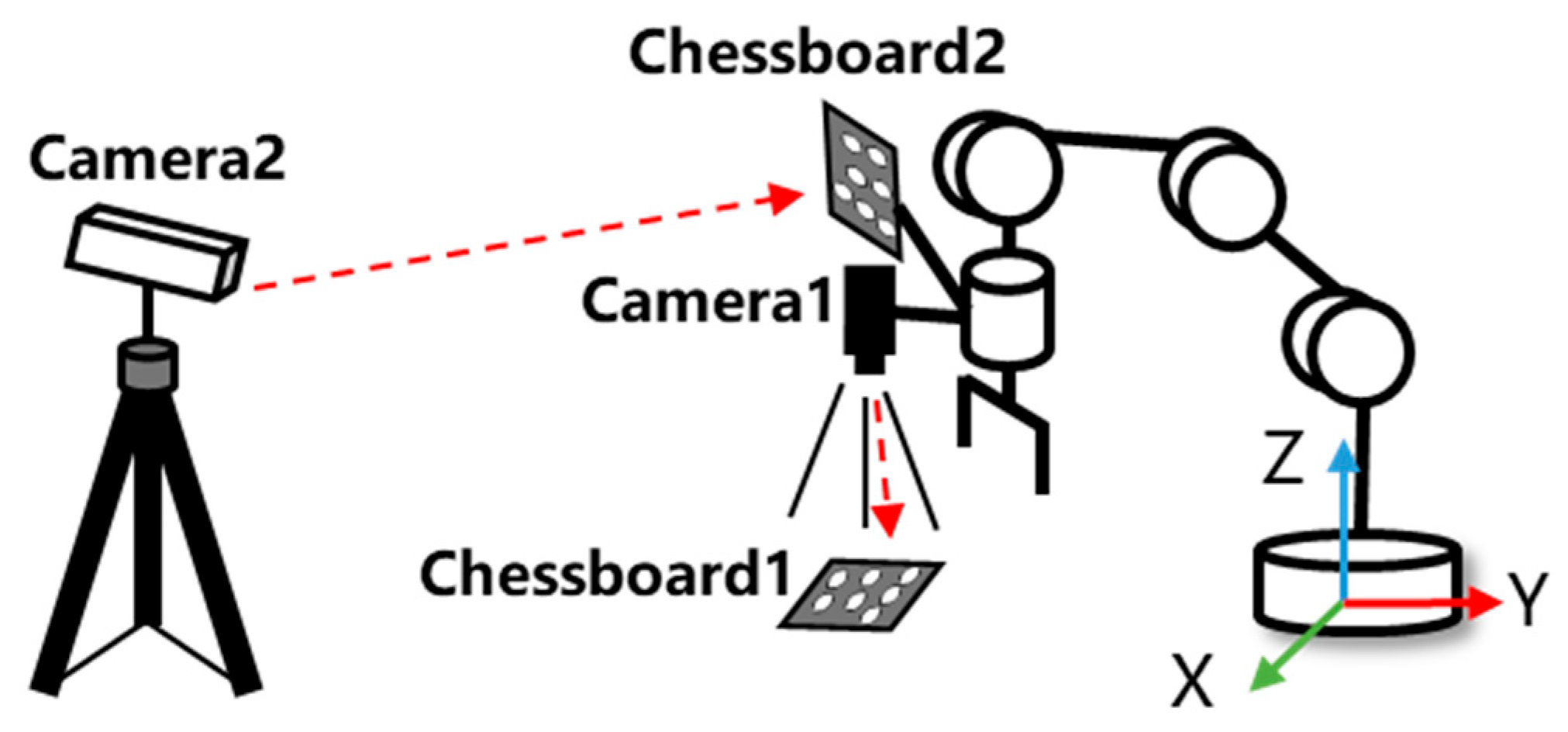
To illustrate our visual servoing strategy, a system consisting of two cameras and one seven-degree-of-freedom robot will be studied first. The entire system is shown in Figure 2. We define the camera fixed at the end of the robot moving with the robot as Camera 1, with a photocentric coordinate system of { C 1 } ; the camera fixed on the experimental platform and not moving is defined as Camera 2, with a photocentric coordinate system of { C 2 } . The coordinate system of the base of the robot is { B } , and the end of the robot is { E } . The red dashed arrows indicate the positions where the cameras observe the corresponding features.
In this paper, we focus solely on spatial motion; therefore, we assume that the orientation of the end-effector remains constant (i.e., no rotational motion), while translational motion is still permitted for spatial positioning. This assumption, together with the orthogonal placement, results in the relative positions of Camera 1 and Camera 2 being approximately orthogonal. Consequently, to decouple the three-dimensional spatial motion, we utilize the two cameras to control spatial motion in different directions. Based on the relative positional relationships between the various components of the system, we have positioned the fixed Camera 2 at a greater distance to guide the robotic arm’s movement in the Z-direction, whilst the end-effector camera, Camera 1, is aligned with the experimental platform to guide the robot’s movement in the X and Y directions.
The key insight behind this orthogonal configuration is that the spatial motion is naturally decoupled into planar and depth components. In conventional IBVS, a full-rank interaction matrix couples all velocity components, which often leads to singularities or local minima when the initial image error is large. By assigning Camera 1 to govern the XY motion and Camera 2 to govern the Z motion, we reduce the effective dimensionality of each sub-controller. This not only simplifies the interaction matrices (as will be shown in Section 3.2) but also expands the region of convergence, because the two lower-dimensional control problems are less likely to be trapped in local minima than a single high-dimensional one. Moreover, sequencing the motions—first converging in the XY-plane, then moving in all three directions—further improves stability by preventing simultaneous large errors in all axes from corrupting the velocity command.
To facilitate the extraction of feature information from the robot’s end-effector and the workpiece on the experimental platform, Chessboard 1 is mounted on the experimental platform, with a coordinate system of { M 1 } , and Chessboard 2 is mounted on the robotic arm’s end-effector, with a coordinate system of { M 2 } . In this configuration, Camera 1 observes Chessboard 1, whilst Camera 2 observes Chessboard 2. Compared with binocular stereo vision, which requires both cameras to simultaneously observe the same target and suffers from limited depth accuracy due to baseline constraints, our orthogonal hybrid configuration offers two distinct advantages:
First, the Z-axis is controlled directly by the independent eye-to-hand camera (Camera 2) using a high-resolution pattern, decoupled from the XY motion. This eliminates the triangulation error inherent in binocular systems and provides higher depth precision.
Second, since the two cameras track different targets (workpiece vs. end-effector) rather than the same target, there is no requirement for a common field-of-view. Consequently, the robot is free to move over a much larger workspace without losing visual feedback, whereas binocular vision would force the end-effector to stay within the limited overlapping field-of-view of both cameras.
These features make the proposed system more suitable for industrial tasks that require both high spatial accuracy and a large operational range.
Once the size of the chessboards has been specified, OpenCV can be used to directly extract corner features and calculate spatial positions, thereby enabling control in different directions.

3.2. Visual Servoing Method

Before deriving the interaction matrices, we define the coordinate frames used throughout this section. Let u , v denote the image pixel coordinates (dimensionless). The camera coordinate frame is denoted as { C } with axes X C , Y C , Z C , where Z C is the optical axis. The robot base coordinate frame is { B } , and the end-effector frame is { E } .
IBVS aims to minimize the error e :
e ( t ) = s s
where s is the visual feature vector in the image plane. s is the target value of the visual feature. We consider the case when the target s is stationary. For both eye-in-hand and eye-to-hand cameras, the change in s depends only on the movement of the end of the robot.
After the target s has been determined, the velocity controller is designed to establish the relationship matrix between the current value of the visual feature s and the camera velocity, defining the camera velocity vector as v c = [ ν c T , ω c T ] T :
s ˙ = L v c
where L is interaction matrix, the relationship between the error vector e and the camera velocity vector is expressed as:
e ˙ = L v c
The control law can be obtained by taking the velocity v c as an input to the robot control and making the error e decay exponentially ( e ˙ = λ e , λ > 0 ):
v c = λ L + e
where L + is the Moore–Penrose pseudoinverse of L , since L may not be full rank.
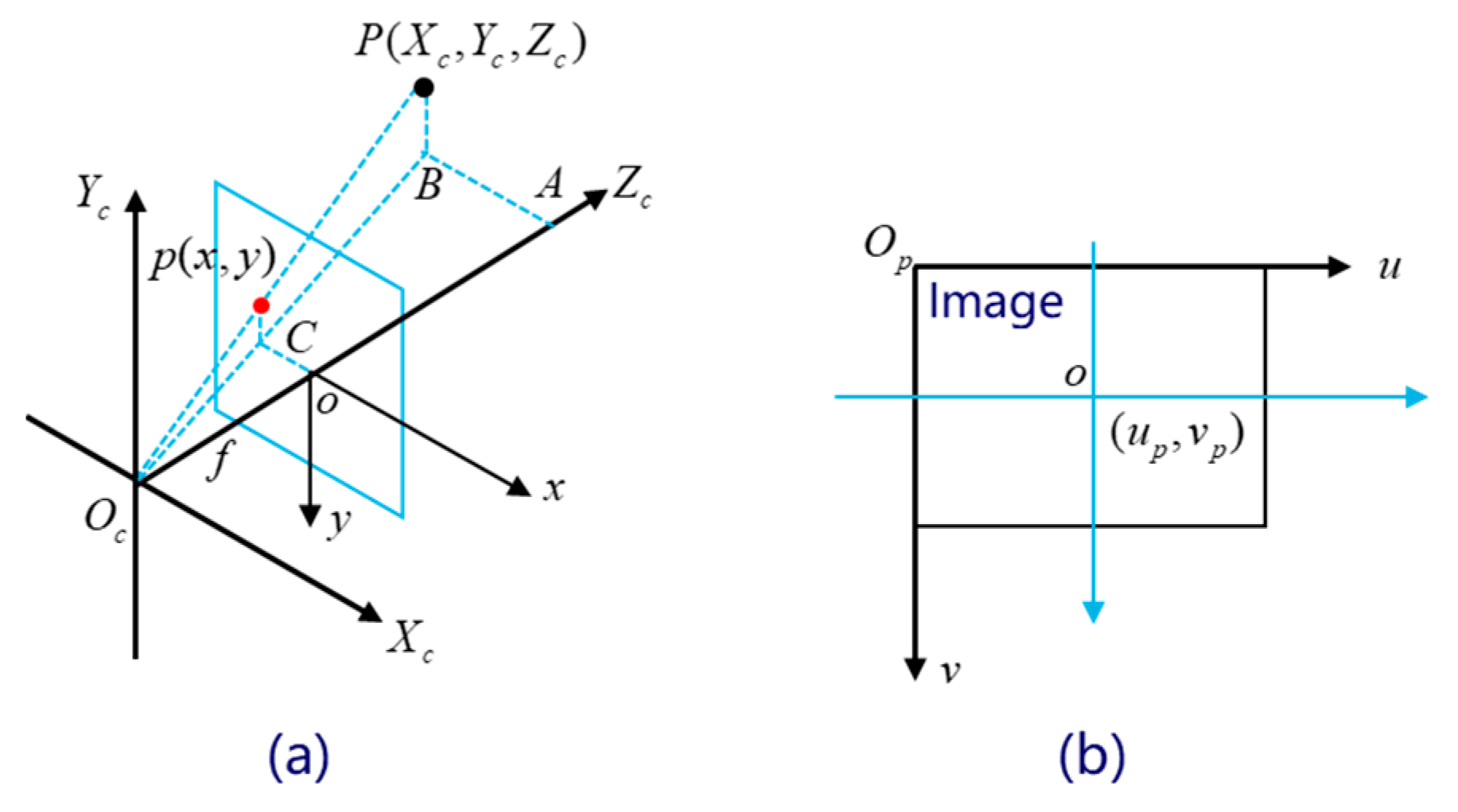
Therefore, to obtain the control command for the robot’s velocity, we need to derive the interaction matrix L (see Figure 3).
From the principle of small hole imaging, the transformation of a spatial point from the camera coordinate system to the image coordinate system is:
Z C x y 1 = f 0 0 0 f 0 0 0   1 X C Y C Z C
The transformation relationship between the image pixel coordinate system and the image physical coordinate system is:
u v 1 = 1 d x 0 u 0 0 1 d y ν 0 0 0 1 x y 1
where d x and d y denote the physical size of each pixel in the x and y directions, respectively. Based on the calibrated internal references, f x = f d x , f y = f d y . Additionally, ( u 0 , v 0 ) represents the coordinates of the pixel center. Substituting (12) into (11) yields:
Z C u v 1 = f x 0 u 0 0 f y ν 0 0 0 1 X C Y C Z C
When fixing the camera and moving the spatial point, the velocity relation is:
p ˙ c = v p + ω p × p c
When fixing the spatial point and moving the camera, the velocity relation is:
p ˙ c = v c ω c × p c
To illustrate the interaction matrix L , a camera with eye-in-hand can be derived via (15):
X ˙ C = v c , x ω c , y Z C + ω c , z Y C Y ˙ C = v c , y ω c , z X C + ω c , x Z C Z ˙ C = v c , z ω c , x Y C + ω c , y X C
The velocity relationship between pixel points and spatial points can be obtained by substituting (16) into (13):
u ˙ v ˙ = f x Z C 0 ( u u 0 ) Z C ( u u 0 ) ( v v 0 ) f y f x 2 + ( u u 0 ) 2 f x f x ( v v 0 ) f y 0 f y Z C ( v v 0 ) Z C f y 2 + ( v v 0 ) 2 f y ( u u 0 ) ( v v 0 ) f x f y ( u u 0 ) f x v c , x v c , y v c , z ω c , x ω c , y ω c , z
So for each pixel point, the interaction matrix L is:
L = f x Z C 0 ( u u 0 ) Z C ( u u 0 ) ( v v 0 ) f y f x 2 + ( u u 0 ) 2 f x f x ( v v 0 ) f y 0 f y Z C ( v v 0 ) Z C f y 2 + ( v v 0 ) 2 f y ( u u 0 ) ( v v 0 ) f x f y ( u u 0 ) f x
In this paper, the focus is primarily on the spatial positioning control of the robot; therefore, orientation control is not considered. In this case, the interaction matrix may omit the orientation component and be simplified as follows:
L = f x Z C 0 ( u u 0 ) Z C 0 f y Z C ( v v 0 ) Z C
Based on the design of the orthogonal visual system, Camera 1, which is mounted on the robot, primarily guides the robot within the XY plane of the experimental platform. Therefore, the corresponding interaction matrix and velocity for Camera 1 are:
L x y = f x 1 Z 1 0 0 f y 1 Z 1 v C 1 C 1 = λ L x y + e 1
Here, L x y 2 × 2 is the interaction matrix for Camera 1, derived from (18) by retaining only the translational velocity components in the XY-plane and assuming zero orientation and zero Z-axis motion. Because the target (Chessboard 1) is planar and placed parallel to the image plane, depth Z 1 is approximately constant, and L x y is full rank.
As for Camera 2, which is positioned outside the hand, it only moves in the Z-axis, so the control can be simplified as follows:
L z = f y 2 Z 2 v E C 2 = λ 2 L z + e 2
Here L z is a non-zero scalar because the feature displacement is monotonic with depth; its exact value depends on the camera intrinsics and the current depth Z 2 . As long as the target remains in view, L z 0 and the Z-axis control is well defined.
In particular, the depth features of the two cameras can be obtained by recognizing the chessboard pattern.
It is worth noting that by decoupling the motion directions, the interaction matrices in (20) and (21) contain only the components relevant to the respective cameras. This avoids the coupling terms that typically cause singularities and local minima when a full matrix is used with large initial feature errors. As a result, the controller remains well-conditioned even when the robot starts far from the target, thereby enlarging the practical convergence domain.
Furthermore, the velocities calculated above are all in the camera coordinate system; however, for robot control, these must be transformed into the robot’s base coordinate system so that they can be directly interpreted as commands by the robot. Therefore, the two velocities derived above are transformed into the robot’s base coordinate system:
v E ( x , y ) B = A d ( T E B ) A d ( T C 1 E ) v C 1 C 1 v E ( z ) B = R C 2 B 0 0 R C 2 B v E C 2
where A d ( T ) denotes the adjoint transformation of T ; T C 1 E denotes the transformation matrix from { C 1 } to { E } ; T E B denotes the transformation matrix from { E } to { B } ; R C 2 B denotes the rotation matrix from { C 2 } to { B } ; v E ( x , y ) B denotes the velocity influenced by the X and Y directions; and v E ( z ) B denotes the velocity influenced by the Z direction. In particular, to ensure dimensional alignment, v C 1 C 1 and v E C 2 are temporarily extended to six dimensions, denoted as v C 1 C 1 and v E C 2 :
v C 1 C 1 = v C 1 C 1 ( 1 ) v C 1 C 1 ( 2 ) 0 0 0 0 T v E C 2 = 0 0 v E C 2 0 0 0 T
where v ( i ) denotes the value at the i-th position of the vector v .
Combine the components in the corresponding directions, once the calculations are complete, to form the final robot velocity v E B :
v E B = v E ( x , y ) B + v E ( z ) B
Clearly, provided that the robot’s end-effector orientation remains constant and the two cameras remain roughly orthogonal to one another, the robot’s velocity can be approximated as:
v E B = v C 1 C 1 ( 1 ) v C 1 C 1 ( 2 ) v E C 2 T
To ensure the safety and stability of the operation, the speeds generated by the two cameras are controlled separately in this design. The robot will first move along the XY axes; once the pixel error in the XY direction falls below the set threshold, it will then move along the XYZ axes simultaneously.
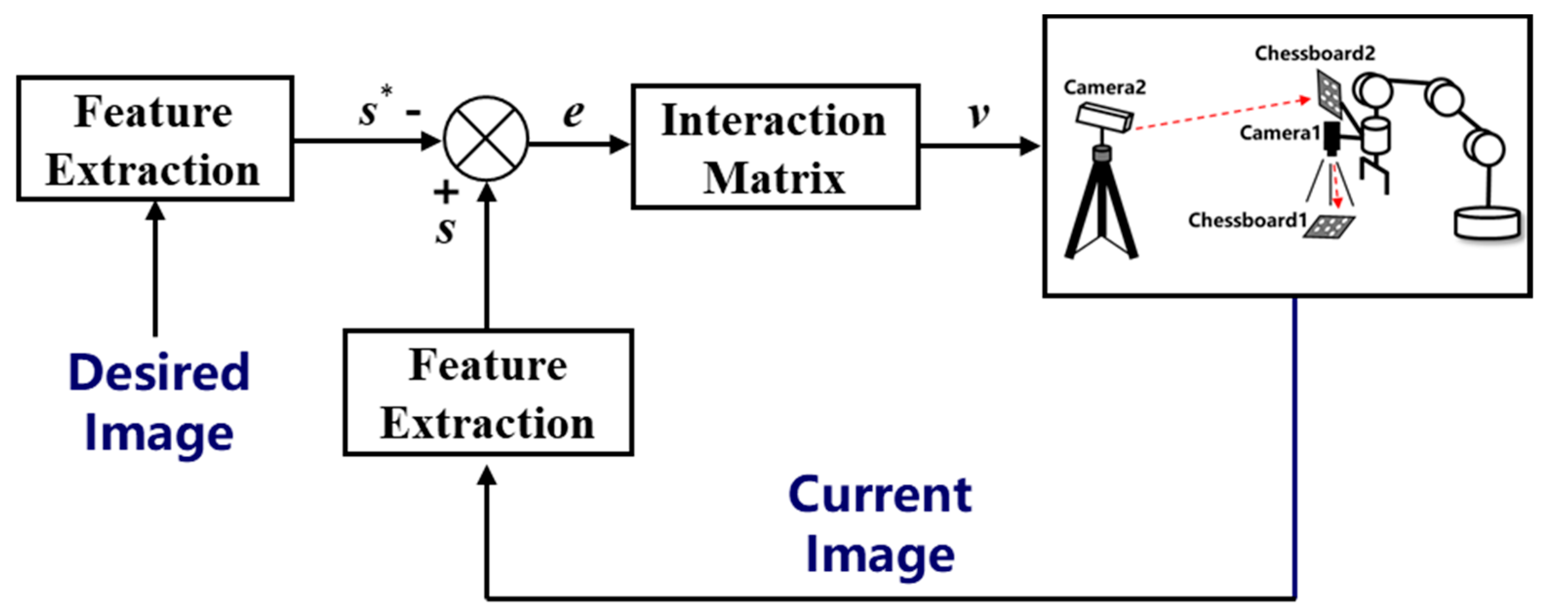
The control strategy of the visual servoing is shown in Figure 4. Within each iteration, the two cameras extract visual features from the chessboard; after calculating the visual deviation relative to their respective target images, the resulting velocities are added together to obtain the final velocity. This process is repeated until the visual deviation falls below a set threshold.

3.3. Stability Analysis of the Decoupled IBVS Controller

In this section, we provide a formal Lyapunov-based stability analysis for the proposed decoupled visual servoing controller. The analysis assumes that the two cameras are approximately orthogonal and that the end-effector orientation remains constant, as stated in Section 3.1. Under these assumptions, the overall spatial motion is decoupled into two independent subsystems: an XY-plane subsystem controlled by Camera 1 (eye-in-hand) and a Z-axis subsystem controlled by Camera 2 (eye-to-hand).
Consider the Lyapunov candidate function:
V = 1 2 e T e
Its time derivative along the closed-loop dynamics is:
V ˙ = e T e ˙
For a stationary target, the time derivative of the error is related to the camera velocity by e ˙ = L v c . Substituting the control law gives:
e ˙ = L v = λ L L + e
In the ideal case where the interaction matrix is exactly known (i.e., L ^ = L ), we have L L + = I when L is full rank. Hence
e ˙ = λ e , λ > 0
therefore:
V ˙ = e T ( λ e ) = λ e 2 0
This yields exponential convergence of the image error to zero:
e ( t ) = e ( 0 ) e λ t
In practice, small calibration errors or non-perfect orthogonality may cause a mismatch between L and its estimate. In that case, the closed-loop system becomes e ˙ = λ L L + e . Provided that the matrix L L + is positive definite (which holds for sufficiently small calibration errors), the equilibrium e = 0 remains asymptotically stable.
Because the two stages are executed sequentially, the overall system inherits the exponential convergence of each stage. The staged design offers two important theoretical advantages. First, it avoids the local minima and singularities that often plague fully coupled 3-DOF IBVS, since each stage operates in a low-dimensional subspace (2DOF then 1DOF). Second, the practical convergence domain is significantly enlarged: the XY stage can converge from arbitrarily large initial image errors (as long as the target remains visible), and the subsequent Z stage does not disturb the already-converged XY position due to the approximately orthogonal configuration (residual coupling is bounded, as analyzed in Section 3.4). In practice, small calibration errors or non-perfect orthogonality may introduce bounded perturbations, but the equilibrium remains asymptotically stable for sufficiently small deviations. This analysis together with the experiments in Section 4 confirms that the proposed method achieves stable and accurate spatial localization from distant initial poses.

3.4. Sensitivity to Orthogonality Deviation

In our control strategy, the robot first converges in the XY-plane using only Camera 1 (eye-in-hand), and then moves along the Z-axis using only Camera 2 (eye-to-hand). Therefore, the effect of a small deviation from perfect orthogonality between the two cameras is relevant only during the second stage (Z-axis motion).
Let the actual rotation between Camera 2 and Camera 1 frames deviate from the ideal orthogonal configuration by a small angle vector θ = θ x , θ y , θ z T . Because Camera 2 is fixed and its target (Chessboard 2) moves with the robot end-effector, the desired pure Z-axis motion (velocity v E ( z ) B in the robot base frame) will, due to the misalignment, appear as a small velocity in the XY-direction in the image plane of Camera 2. Specifically, the interaction matrix of Camera 2, which under ideal orthogonality would have only a Z-component, now obtains off-diagonal terms.
Consequently, when the controller commands a pure Z-axis velocity, the actual closed-loop system induces a small residual XY velocity proportional to θ . Using the same Lyapunov function V = 1 2 e T e for the XY errors during the second stage, one can show that the final XY positioning error remains bounded by a constant proportional to θ / k , where k is the controller gain.
For small deviations (e.g., θ < 5 ° ), the induced XY error is below the measurement noise level. For larger deviations (>10°), the residual error becomes non-negligible, and the ideal staged control strategy should be replaced by a fully coupled controller that compensates for the cross-coupling. This analysis justifies that the proposed method tolerates normal mounting inaccuracies without performance degradation, as verified by our experiments in Section 4, where the two cameras were aligned manually with an estimated error within ±5°.

4. Experimental Results and Discussion

To validate the effectiveness of the proposed method, we carried out high-precision spatial localization experiments on a robot guided by the orthogonal camera-based visual servoing system, following the procedures described in Section 2 and Section 3.
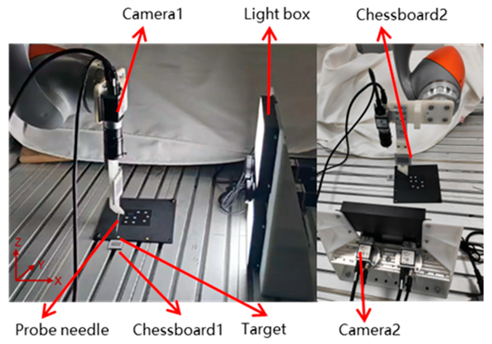
As shown in Figure 5 for our experimental scenario, along with the choice of the robot KUKA iiwa (KUKA AG, Augsburg, Germany), the two Basler industrial cameras (Basler AG, Ahrensburg, Germany; resolution 1920 × 1080) are placed orthogonally: Camera 1 is fixed at the end of the robot along with the movement of the robot, and Camera 2 is fixed to the experimental platform. The controller ran on a standard PC (Intel Core i7-8700, 16 GB RAM, RTX 4060). The control loop was set to a fixed frequency of 10 Hz. Timing measurements over 500 consecutive control cycles showed that image acquisition and sub-pixel corner extraction (including distortion correction) took 70–80 ms, while the velocity computation (interaction matrix pseudo-inverse and transformation to robot base coordinates) took less than 10 ms. The total cycle time was approximately 90 ms, well within the 100 ms period. Table 1 lists the key experimental parameters and implementation details.
A small hole on the experimental platform was filled with playdough to simulate a workpiece. A probe needle was fixed at the robot’s end-effector; the needle was then used to poke the playdough so that the spatial positioning accuracy could be evaluated by comparing the needle hole with the original hole. In order to verify the high accuracy of the method and ensure the simplicity of the experiment, we choose a standard chessboard as the target and extract its sub-pixel corners as the target points used by the visual servoing algorithm, in which Chessboard 1 is fixed next to the playdough hole, which can be regarded as the bias of the playdough hole, and Chessboard 2 is fixed next to the probe needle at the end of the robot, which can be regarded as the bias of the probe needle. Camera 1 in the experimental process needs to ensure that Chessboard 1 visible, and is used to locate the XY position of the playdough hole. Camera 2 in the experimental process needs to ensure that Chessboard 2 visible, and is used to locate the Z position of the playdough hole.
Before the start of the experiment, the two cameras are subjected to internal parametric calibration and hand–eye calibration, where hand–eye calibration only requires the acquisition of 5–10 pictures, because the image-based visual servoing is robust enough to hand–eye calibration errors. Then the robot is moved by the oscillator so that the probe needle leaves a small hole in the playdough and the position of the corner point of Chessboard 1 in Camera 1 is extracted as the target point in the XY direction at this time and the position of the corner point of Chessboard 2 in Camera 2 is extracted as the target point in the Z direction. After moving the robot away, the distortion coefficients obtained from the internal parameter calibration are used to undistort the image and extract the sub-pixel corner points of the current chessboard in real time, and the speed of the end of the robot is directly calculated by the pseudo-inverse of the interaction matrix derived in Section 3. For the sake of safety and stability, we first move along the XY direction, and then move along the XYZ simultaneously when the pixel point error in the XY direction is smaller than the threshold we set. When the distance between the pixel point extracted from the two cameras and the target point is less than a certain value, we end the positioning movement, and if the corner point is obscured during the process, we set the movement speed to 0 to avoid flying accidents.
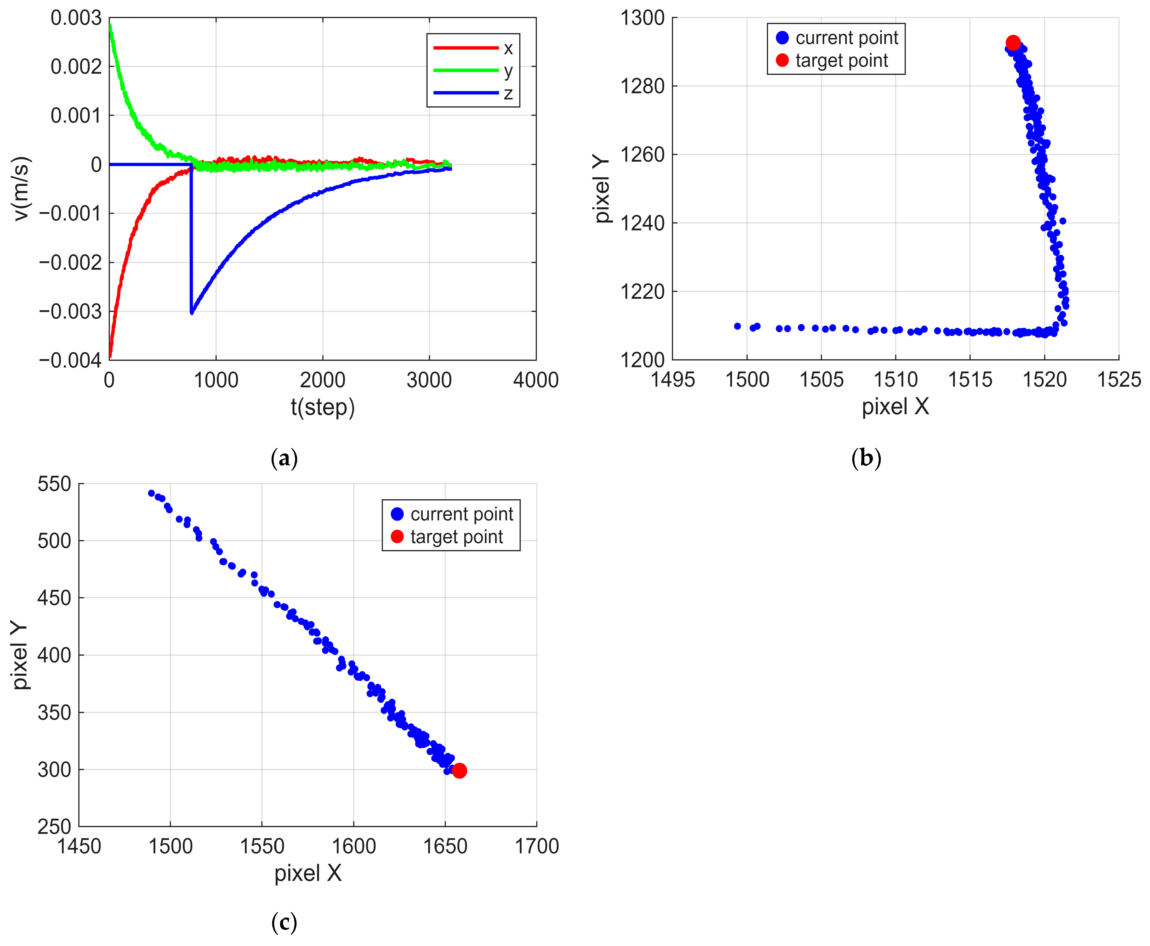
Figure 6 shows the output motion speed in the XYZ direction and the position of the target point extracted during the experiment. The computed velocity is proportional to the current pixel error, scaled by the gain λ (see Section 3.2) and the pseudo-inverse of the interaction matrix. The resulting linear velocity commands are expressed in m/s, and the robot controller executes them directly. Every time a corner point is extracted, the velocity output is calculated through the interaction matrix, and it can be found that the closer to the target pixel point, the smaller the velocity is, until it approaches 0.
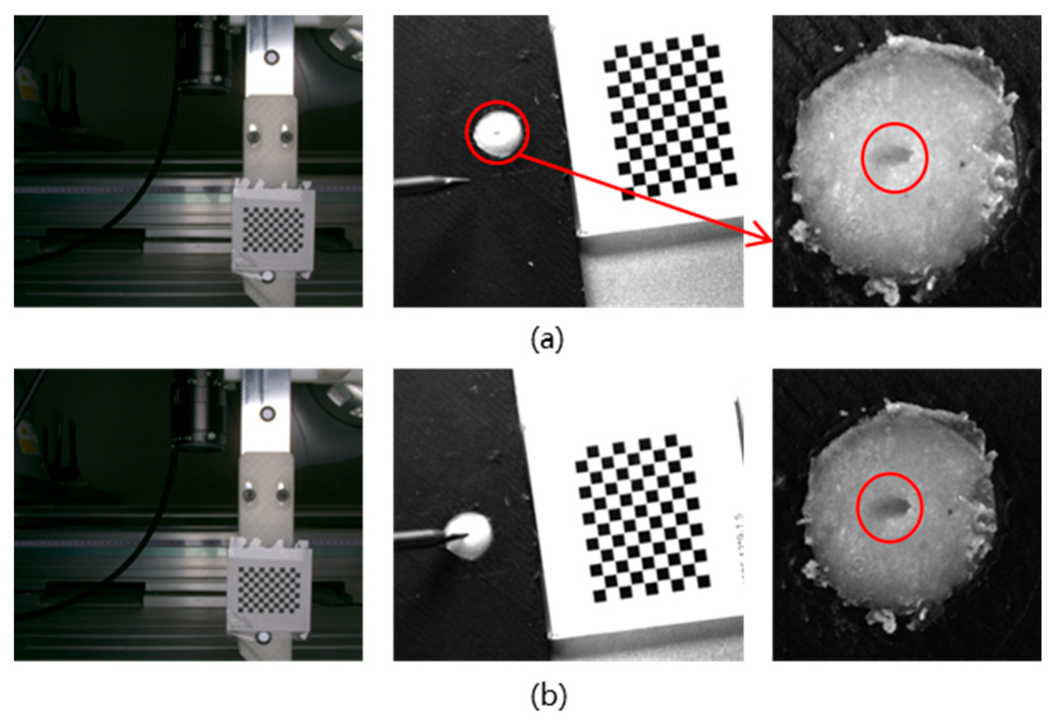
Figure 7a is the picture taken at the beginning of the experiment, in which the left one is the picture taken by Camera 2, and the middle one is the picture taken by Camera 1, both of which can observe the complete chessboard, and the right one is the enlarged picture of the playdough hole, and the red circle in this image indicates the initial indentation made by the probe needle at the beginning of the experiment. Figure 7b is the picture taken at the end of the positioning; it can be seen that the end of the robot is descending along the Z direction, and the probe needle is back to the position of the playdough hole poked before the beginning of the experiment, and the holes of the probe needle can be seen to be almost completely overlapped by the enlarged holes of the playdough hole at the two times, and the red circle in the right image of Figure 7b indicates the indentation after the experiment; compared with the initial indentation in Figure 7a, the post-experimental indentation shows deeper marks within the same red-circled small area, and the two indentations almost completely overlap. The alignment of the probe needle with the playdough hole was inspected visually using the camera images and under magnified observation. Based on the recorded images, the residual XY offset was estimated to be within approximately 0.02 mm (limited by the camera resolution of about 0.05 mm per pixel in the working area and manual judgement), and the Z-axis error was estimated to be within 0.04 mm. Therefore, the overall spatial localization error is conservatively reported as less than 0.05 mm. It should be noted that these error estimates are approximate; a calibrated external measurement system (e.g., a laser tracker) would be required to determine the absolute accuracy. Within the limitations of our experimental setup, the achieved repeatability of 0.05 mm validates the proposed visual servoing method.

5. Conclusions and Future Works

In this paper, a high-precision spatial visual servoing system based on a hybrid orthogonal camera configuration has been developed. By integrating an eye-in-hand camera and an eye-to-hand camera and employing directionally decoupled interaction matrices, the robot’s spatial motion is controlled separately in the XY-plane and along the Z-axis. This decoupling strategy effectively expands the convergence domain of image-based visual servoing and achieves stable convergence from a distant initial pose in our experiments, which can reduce the likelihood of local minima and singularities compared to conventional coupled IBVS, as suggested by the decoupled structure and observed in our experiments. Firstly, the intrinsic calibration and hand–eye calibration of the two orthogonally placed cameras are carried out, and the accuracy of hand–eye calibration is not too demanding; then the sub-pixel level image position of the target is extracted in real time, the interaction matrix is derived, and the linear controller is designed to control the robot’s motion; finally, an experiment of spatial localization with an accuracy of 0.05 mm is completed on the KUKA iiwa, which verifies the validity and robustness of the method under normal indoor lighting conditions. We acknowledge that the current experimental validation is limited to a single initial pose without repeated trials or statistical analysis; a more thorough evaluation with multiple initial positions and distances is needed to fully demonstrate robustness and generalizability.
In the future, although a chessboard pattern was used as the visual target in our experiments for its convenience and repeatability, the proposed method is not inherently limited to chessboard features. Any planar pattern with robustly detectable corner or keypoint features (e.g., customized fiducial markers, dot grids, or even natural textures) can serve as the feature target. Such markers can be attached to a real workpiece as long as they remain within the camera’s field of view. In future work, we plan to integrate deep learning-based object detection and keypoint extraction (e.g., YOLO, SuperPoint, or Siamese networks) to eliminate the need for explicit markers, further enhancing the method’s industrial transferability. We also acknowledge that occlusion remains a limitation; future research will investigate occlusion-robust strategies such as using multiple distributed markers or temporal prediction (e.g., Kalman filter) to maintain tracking during partial occlusion. Additionally, the image-based visual servoing algorithms will be improved and more advanced controllers will be introduced, and a high-precision laser tracker will be used to measure the accurate positioning error values.

Author Contributions

Conceptualization, S.C. and X.Z.; methodology, X.G. and S.C.; software, S.C.; validation, X.G. and S.C.; formal analysis, X.G.; investigation, Z.D.; resources, J.T.; data curation, S.N.; writing—original draft preparation, X.G.; writing—review and editing, S.C. and Z.D.; visualization, J.T.; supervision, S.C. and X.Z.; project administration, X.Z.; funding acquisition, X.Z. All authors have read and agreed to the published version of the manuscript.

Funding

This study was supported by the National Key Research and Development Program of China under Grant No. 2023YFB3408603, the National Natural Science Foundation of China Distinguished Young Scientist Fund (No. 52422501), the National Science Foundation for Young Scientists of China (No. 52505018) and the Interdiciplinary Research Program of Hust (No. 2024JCYJ035). It was also sponsored by the Fundamental and Interdisciplinary Disciplines Breakthrough Plan in Humanoid Robotics of the Ministry of Education of China (No. JYB2025XDXM208).

Data Availability Statement

The original contributions presented in the study are included in the article, further inquiries can be directed to the corresponding author.

Conflicts of Interest

Authors Zuoheng Duan, Jiahao Tan andShaodong Nie were employed by the company AVIC Chengdu Aircraft Industrial (Group) Co., Ltd. The remaining authors declare that the research was conducted in the absence of any commercial or financial relationships that could be construed as a potential conflict of interest.

References

  1. Sun, X.; Zhu, X.; Wang, P.; Yang, L.; Li, G.; Liu, B.; Hu, X. A Review of Robot Control with Visual Servoing. In Proceedings of the 2018 IEEE 8th Annual International Conference on CYBER Technology in Automation, Control, and Intelligent Systems (CYBER), Tianjin, China, 19–23 July 2018; pp. 116–121. [Google Scholar] [CrossRef]
  2. Li, S.; Ghasemi, A.; Xie, W.; Gao, Y. An Enhanced IBVS Controller of a 6DOF Manipulator Using Hybrid PD-SMC Method. Int. J. Control Autom. Syst. 2018, 16, 844–855. [Google Scholar] [CrossRef]
  3. Duy Cong, V.; Duc Hanh, L. Combination of Two Visual Servoing Techniques in Contour Following Task. In Proceedings of the 2021 International Conference on System Science and Engineering (ICSSE), Ho Chi Minh City, Vietnam, 26–28 August 2021; pp. 382–386. [Google Scholar] [CrossRef]
  4. Zhao, X.; Emami, M.R.; Zhang, S. Image-Based Control for Rendezvous and Synchronization with a Tumbling Space Debris. Acta Astronaut. 2021, 179, 56–68. [Google Scholar] [CrossRef]
  5. Hanh, L.D.; Cong, V.D. Implement Contour Following Task of Objects with Unknown Geometric Models by Using Combination of Two Visual Servoing Techniques. Int. J. Comput. Vis. Robot. 2022, 12, 464–486. [Google Scholar] [CrossRef]
  6. Wu, J.; Jin, Z.; Liu, A.; Yu, L.; Yang, F. A Survey of Learning-Based Control of Robotic Visual Servoing Systems. J. Frankl. Inst. 2022, 359, 556–577. [Google Scholar] [CrossRef]
  7. Shi, H.; Chen, J.; Pan, W.; Hwang, K.-S.; Cho, Y.-Y. Collision Avoidance for Redundant Robots in Position-Based Visual Servoing. IEEE Syst. J. 2019, 13, 3479–3489. [Google Scholar] [CrossRef]
  8. Sanderson, A.C.; Weiss, L.E. Image-Based Visual Servo Control Using Relational Graph Error Signals. In Proceedings of the IEEE International Conference on Cybernetics and Society, Cambridge, MA, USA, 8–10 October 1980; pp. 1074–1077. [Google Scholar]
  9. Dementhon, D.F.; Davis, L.S. Model-Based Object Pose in 25 Lines of Code. Int. J. Comput. Vis. 1995, 15, 123–141. [Google Scholar] [CrossRef]
  10. Ren, X.L.; Li, H.W. Uncalibrated Image-Based Visual Servoing Control with Maximum Correntropy Kalman Filter. IFAC PapersOnLine 2020, 53, 560–565. [Google Scholar] [CrossRef]
  11. Mezouar, Y.; Chaumette, F. Path Planning for Robust Image-Based Control. IEEE Trans. Robot. Autom. 2002, 18, 534–549. [Google Scholar] [CrossRef]
  12. Li, Y.X.; Mao, Z.Y.; Tian, L.F. Valve Servo Control Based on Artificial Immune and Image Direct Feedback. J. S. China Univ. Technol. 2009, 37, 54–58. [Google Scholar]
  13. Vidyasagar, M. System Theory and Robotics. IEEE Control Syst. Mag. 1987, 7, 16–17. [Google Scholar] [CrossRef]
  14. Lin, J.; Gu, S.; Chen, Q.J. Autonomous Navigation of Mobile Robots Based on Image Visual Servoing. In Proceedings of the Ninth China Intelligent Robot Symposium, Shenzhen, China, 11–13 November 2011; pp. 220–222+231. [Google Scholar]
  15. Li, H.G.; Zhu, X.D.; Li, G.Y. Image Moment Based Adaptive Visual Servoing Robot Control. In China Annual Conference of Control and Decision; Northeastern University Press: Shenyang, China, 2004; pp. 893–895. [Google Scholar]
  16. Feng, Y.W.; Li, J.G.; Guo, G. A Control Method of Soccer Robot Based on Visual Feedback. In Proceedings of the 21st Annual Conference of Young Scholars of Chinese Society of Automation, Yantai, China, 2006; pp. 195–199. [Google Scholar]
  17. Dong, Z.D.; Liu, S.R.; Jiang, H.C. Visual Servo Control of Six-Degree-of-Freedom Manipulator Based on Image Moment and Vector Product Method. J. Univ. Shanghai Sci. Technol. 2013, 221–226. [Google Scholar]
  18. Robinson, L.; Gadd, M.; Newman, P.; Martini, D.D. Robot-Relay: Building-Wide, Calibration-Less Visual Servoing with Learned Sensor Handover Networks. Auton. Robot. 2026, 50, 3. [Google Scholar] [CrossRef]
  19. Pathre, P.; Gupta, G.; Qureshi, M.N.; Brunda, M.; Brahmbhatt, S.; Krishna, K.M. Imagine2Servo: Intelligent Visual Servoing with Diffusion-Driven Goal Generation for Robotic Tasks. In Proceedings of the 2024 IEEE/RSJ International Conference on Intelligent Robots and Systems (IROS), Abu Dhabi, United Arab Emirates, 14–18 October 2024. [Google Scholar]
  20. Xu, F.; Chen, P. Research on Uncalibrated Adaptive Visual Servoing Control Based on Dual-Camera Fusion. Adv. Mech. Eng. 2025, 17, 16878132251374118. [Google Scholar] [CrossRef]
  21. Tian, J.; Zhong, X.; Peng, X.; Hu, H.; Liu, Q. Model-Free Visual Servoing Based on Active Disturbance Rejection Control and Adaptive Estimator for Robotic Manipulation without Calibration. Ind. Robot 2024, 51, 820–836. [Google Scholar] [CrossRef]
  22. Zhang, Y.; Manzoor, S.; Joo, K.J.; Kim, S.M.; Kuc, T.Y. Robust Adaptive Repetitive Learning Control for Manipulators with Visual Servoing. Mechatronics 2024, 96, 103121. [Google Scholar] [CrossRef]
  23. Chen, Z.; Wen, W.; Yang, W. Adaptive Visual Control for Robotic Manipulators with Consideration of Rigid-Body Dynamics and Joint-Motor Dynamics. Mathematics 2024, 12, 2413. [Google Scholar] [CrossRef]
  24. Zhou, Y. Based on Image Uncalibrated Mixing Binocular Visual Servo for Manipulator. Master’s Thesis, Chongqing University, Chongqing, China, 2016. [Google Scholar]
  25. Zhang, Z. A Flexible New Technique for Camera Calibration. IEEE Trans. Pattern Anal. Mach. Intell. 2000, 22, 1330–1334. [Google Scholar] [CrossRef]
  26. Tsai, R.Y.; Lenz, R.K. A New Technique for Fully Autonomous and Efficient 3D Robotics Hand/Eye Calibration. IEEE Trans. Robot. Autom. 1989, 5, 345–358. [Google Scholar] [CrossRef]
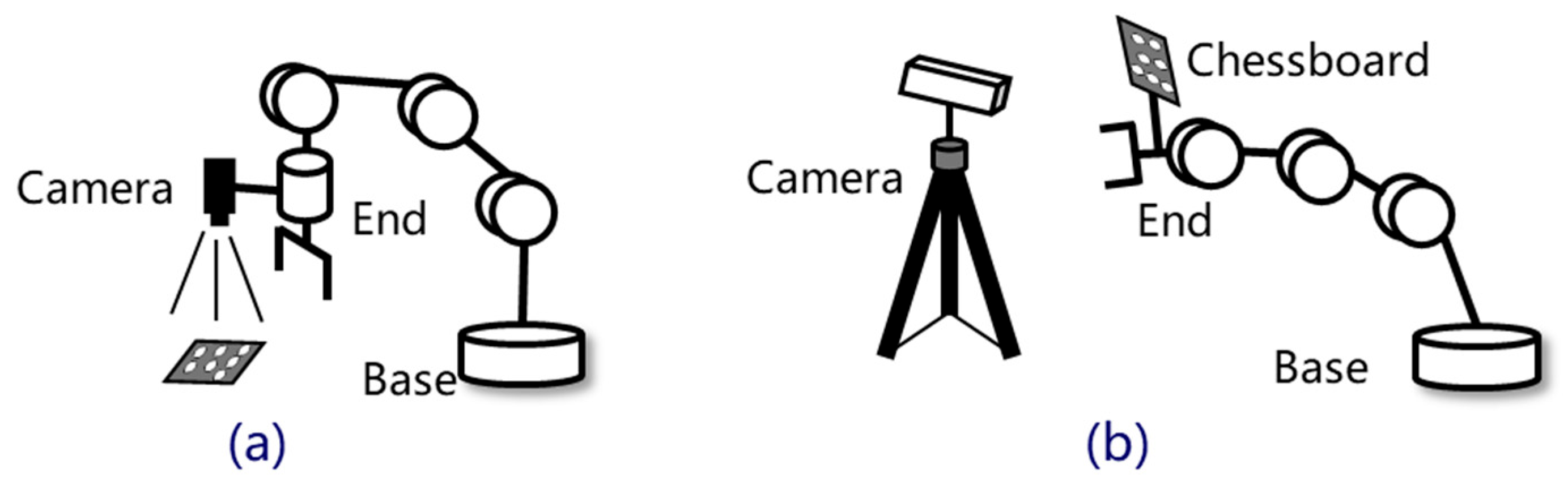
Figure 1. Two hand–eye calibration settings and coordinate system relationships: (a) eye-in-hand and (b) eye-to-hand.
Mathematics 14 02044 g001
Figure 2. Orthogonal visual system.
Mathematics 14 02044 g002
Figure 3. (a) Relationship between space point and camera coordinate system. (b) Relationship between the camera plane coordinate system and the image coordinate system.
Mathematics 14 02044 g003
Figure 4. Block diagram of the control system.
Mathematics 14 02044 g004
Figure 5. Experimental scenario.
Mathematics 14 02044 g005
Figure 6. Experimental process data. (a) XYZ direction velocity. (b) XY plane target pixel position. (c) Z plane target pixel position.
Mathematics 14 02044 g006
Figure 7. Experimental result. (a) Before the start of the experiment. (b) Spatial location results.
Mathematics 14 02044 g007
Table 1. Experimental parameters and implementation details.
Camera ResolutionLens TypeFrame RateChessboard Size
1920 × 1080focal length: 8 mm50 fps12 × 9, 3 mm
Controller GainsStopping CriteriaSampling TimeVelocity Limits
0.0011 pixel0.1 s0.01 m/s
Disclaimer/Publisher’s Note: The statements, opinions and data contained in all publications are solely those of the individual author(s) and contributor(s) and not of MDPI and/or the editor(s). MDPI and/or the editor(s) disclaim responsibility for any injury to people or property resulting from any ideas, methods, instructions or products referred to in the content.