Conformal Mapping and the Finite Element Method

Abstract

One of the interesting properties of the two-dimensional potential problem is that solutions of the Laplace equation remain solutions of the Laplace equation when subjected to a conformal transformation. While this result was established long ago, the consequences within computational mechanics have not been fully explored. Here, we demonstrate for the first time that in a finite element formulation of the potential problem, the stiffness matrix remains invariant under a conformal mapping. This holds even when the mapped domain extends to infinity. Furthermore, by introducing the local flux in a finite element method, we find that the fundamental boundary eigensolutions also are invariant under a conformal mapping transformation by using a special weight function related to the Jacobian of the transformation. A series of computational examples is presented to emphasize the most important characteristics of conformal mappings within the finite element method and to demonstrate convergence of the computational results. Included are two exterior problems, the latter of which permits determination of the tearing stress intensity factor for a crack in an infinite plate.

1. Introduction

Conformal mapping has been used to solve a wide range of two-dimensional boundary value problems, such as potential and elastostatic problems [1,2]. For simply connected regions, the domains are often transformed conformally to a circular domain, which is easier to solve analytically. Infinite domains with a single boundary can be handled similarly.

More recent computational studies connecting conformal mapping with finite element methods include the work by Sumant et al. [3] on electrostatic analysis of MEMS devices, by Costamagna and Di Barba [4] on inhomogeneous dielectrics, by Wu and Chen [5] on variational analysis of dielectric waveguides, by Yang and Lee [6] variational calculation of cutoff wavenumbers in circular eccentric guide, by Nakasumi and Harada [7] on modelling the singularity of the capacitor edge, by Louhghalam et al. [8] on analysis of stress concentrations, by Reck et al. [9] on solving the Helmholtz equation in complex domains, by Legatiuk and Weisz-Patrault [10] and Zhuang et al. [11] on crack propagation, by Xu et al. [12] on shape and topology optimization for thermal problems, and by Mirahki et al. [13] on magnet shape optimization. Some other interesting works are Tang et al. [14], Chakraborty et al. [15], Kropf et al. [16], and Hakul and Rasila [17].

This paper shows for the first time that the stiffness matrix, developed from a standard finite element method, is invariant in a conformal mapping transformation for the potential problem governed by the Laplace equation. It is perhaps surprising that this property has not been recognized previously, as the case of linear transformation (i.e., any combination of translation, rotation, and stretching) is easily verified by looking at the stiffness matrix (or conductance matrix in heat conduction) derived for a single element. More generally, the stiffness matrix for an internal unit circle can be used directly for other simply connected domains or infinite domains, when the analytical forms of the conformal transformations are provided. Alternatively, computational techniques for conformal mapping can be employed. Initially, Symm [18,19,20] developed numerical methods based on integral equations, while finite element approaches have been defined more recently by Nitsche [21] and Tsuchiya [22]. Consequently, the requirement for a closed-form conformal mapping has been alleviated through the introduction of numerical conformal mapping (NCM).

Furthermore, we connect these results to the theory of fundamental boundary eigensolutions [23,24], which shows that under a conformal transformation, we can have invariant eigensolutions provided we use a special weight function related to the Jacobian of the transformation. This requires that, in a finite element method, we use local fluxes as nodal values, contrary to traditional finite element approaches that employ local (lumped) sources as nodal values. By doing so, we generate a second finite element matrix, called the weighted boundary matrix. Invariance of the fundamental boundary eigensolutions under conformal mapping means that the stiffness and weighted boundary matrix are both invariant.

A brief overview of some classical results for conformal mapping in potential theory is provided in the following section. Then, in Section 3, we examine the interesting behavior of the two-dimensional stiffness matrix under a conformal transformation. The connection with the fundamental boundary eigenproblem and the flux-oriented finite element method is formulated afterwards in Section 4 and Section 5, respectively. Having completed the theoretical development, attention shifts in Section 6 to the presentation of computational results that illustrate these features of conformal mappings within the context of a finite element approach. In perhaps the most interesting of these applications, the stiffness matrix from the interior of a circular disc is used directly to solve the anti-plane fracture mechanics problem of a cracked infinite plate. Finally, a summary and some concluding remarks are given in Section 7. For completeness and clarity, Appendix A provides a list of symbols.

2. Conformal Mapping

If the point transformation between the corresponding regions in the $x_1{x}_2$- and $x_1^{\prime }{x}_2^{\prime }$-planes has the property that infinitesimal configurations in $x_1{x}_2$ and their image in $x_1^{\prime }{x}_2^{\prime }$ are arbitrarily close to being similar, the transformation is said to be conformal [2]. The present section summarizes some well-known properties of conformal transformations and provides nomenclature that will be used in the subsequent development.

Let $z^{\prime }=\Omega \left(z\right)$ define a conformal transformation from point $z=x_1+i{x}_2$ in domain $A$ with boundary $S$ to point $z^{\prime }=x_1^{\prime }+i{x}_2^{\prime }$ in domain $A^{\prime }$ with boundary $S^{\prime }$, where $\Omega \left(z\right)$ is a single-valued analytic function. The equations of the transformations can be solved (at least theoretically) for $x_1$ and $x_2$ as single-valued functions of $x_1^{\prime }$ and $x_2^{\prime }$ when the transformation has a single-valued inverse. This implies that the Jacobian determinant of the transformation $J$ is non-zero, where

$$J\left({\displaystyle \frac{x_1^{\prime },x_2^{\prime }}{x_1,x_2}}\right)=\left|\begin{array}{cc}{\displaystyle \frac{\partial x_1^{\prime }}{\partial x_1}}& {\displaystyle \frac{\partial x_1^{\prime }}{\partial x_2}}\\ {\displaystyle \frac{\partial x_2^{\prime }}{\partial x_1}}& {\displaystyle \frac{\partial x_2^{\prime }}{\partial x_2}}\end{array}\right|$$

(1)

Since $z^{\prime }=\Omega \left(z\right)$ is assumed to be analytic, the functions $x_1^{\prime }\left(x_1,x_2\right)$ and $x_2^{\prime }\left(x_1,x_2\right)$ must satisfy the Cauchy–Riemann equations

$${\displaystyle \frac{\partial x_1^{\prime }}{\partial x_1}}={\displaystyle \frac{\partial x_2^{\prime }}{\partial x_2}},\hspace{1em}{\displaystyle \frac{\partial x_1^{\prime }}{\partial x_2}}=-{\displaystyle \frac{\partial x_2^{\prime }}{\partial x_1}}$$

(2a,b)

After substituting Equation (2a,b) into Equation (1), we obtain

$$J\left({\displaystyle \frac{x_1^{\prime },x_2^{\prime }}{x_1,x_2}}\right)=\left|\begin{array}{cc}{\displaystyle \frac{\partial x_1^{\prime }}{\partial x_1}}& {\displaystyle \frac{\partial x_1^{\prime }}{\partial x_2}}\\ {\displaystyle \frac{\partial x_2^{\prime }}{\partial x_1}}& {\displaystyle \frac{\partial x_2^{\prime }}{\partial x_2}}\end{array}\right|={\left({\displaystyle \frac{\partial x_1^{\prime }}{\partial x_1}}\right)}^2+{\left({\displaystyle \frac{\partial x_2^{\prime }}{\partial x_1}}\right)}^2={\left|{\displaystyle \frac{\partial x_1^{\prime }}{\partial x_1}}+i{\displaystyle \frac{\partial x_2^{\prime }}{\partial x_1}}\right|}^2={\left|{\displaystyle \frac{d\Omega \left(z\right)}{dz}}\right|}^2$$

(3)

Consequently, if $\Omega \left(z\right)$ is analytic, the function $z^{\prime }=\Omega \left(z\right)$ will have a single-valued inverse in the neighborhood of any point where the derivative $\Omega \left(z\right)$ is non-zero.

If in the transformation $z^{\prime }=\Omega \left(z\right)$ the function $\Omega \left(z\right)$ has a singularity at some point in the bounded domain $A$ in $x_1{x}_2$, then the mapped domain $A^{\prime }$ in $x_1^{\prime }{x}_2^{\prime }$ is infinite. It is easily proved that $\Omega \left(z\right)$ must have a simple pole at that point. Assuming for simplicity that $z^{\prime }=\infty$ corresponds to $z=0$, then

$$z^{\prime }=\Omega \left(z\right)={\displaystyle \frac{c}{z}}+\widehat{\Omega }\left(z\right)$$

(4)

where $\widehat{\Omega }\left(z\right)$ is an analytic function, $c$ is a constant, and no other singularities can occur in $A$. Otherwise, the transformation would not be reversible and single-valued.

In the mapping defined by the analytic function $z^{\prime }=\Omega \left(z\right)$, the lengths of infinitesimal segments,$ds$ and $d{s}^{\prime }$, regardless of their direction, are altered by a factor $\left|{\displaystyle \frac{d{z}^{\prime }}{dz}}\right|=\left|{\displaystyle \frac{d\Omega }{dz}}\right|=\left|{\displaystyle \frac{d{s}^{\prime }}{ds}}\right|$, which depends only on the point from which they are drawn. The angles between these infinitesimal segments are also preserved in magnitude and in sense as long as ${\displaystyle \frac{d\Omega \left(z\right)}{dz}}\ne 0$. At any critical point, where ${\displaystyle \frac{d\Omega \left(z\right)}{dz}}=0$, $\mathrm{Arg}{\displaystyle \frac{d\Omega \left(z\right)}{dz}}$ is not defined, and we cannot assert that angles are generally preserved in the transformation. Despite this fact, we can have a finite number of critical points in our transformations to generate crack tips or notches in the mapped domain.

Around any point $z$, infinitesimal areas are altered by the factor ${\left|{\displaystyle \frac{d{z}^{\prime }}{dz}}\right|}^2=J\left({\displaystyle \frac{x_1^{\prime },x_2^{\prime }}{x_1,x_2}}\right)$ and

$$d{A}^{\prime }=JdA$$

(5)

while the relation between infinitesimal segments is

$$d{s}^{\prime }=\sqrt{J}ds=\left|{\displaystyle \frac{d\Omega \left(z\right)}{dz}}\right|ds$$

(6)

As we mentioned previously, solutions of the Laplace equation remain solutions to the Laplace equation when subjected to a conformal transformation. A function possessing continuous second partial derivatives and satisfying the Laplace equation is usually referred to as a harmonic function. We now present a brief derivation of this well-known result, formulated in a manner appropriate for the present investigation.

Assume the function $u\left(x_1,x_2\right)$ is harmonic in the domain $A$ defined in the $x_1{x}_2$ plane. Then

$${\nabla }^{2}u=u_{,\alpha \alpha }=0$$

(7)

Here, standard indicial notation that varies only over (1,2) is used. We consider the potential function in the mapped domain $A^{\prime }$ as $u^{\prime }\left(x_1^{\prime },x_2^{\prime }\right)$, where the point $z^{\prime }=x_1^{\prime }+i{x}_2^{\prime }$ is the map of the point $z=x_1+i{x}_2$ in domain $A$. It is obvious that

$$u^{\prime }\left(x_1^{\prime },x_2^{\prime }\right)=u\left(x_1,x_2\right)$$

(8)

Furthermore,

$${\displaystyle \frac{\partial u}{\partial x_{\alpha }}}={\displaystyle \frac{\partial u^{\prime }}{\partial x_a^{\prime }}}{\displaystyle \frac{\partial x_a^{\prime }}{\partial x_{\alpha }}}$$

(9)

$${\displaystyle \frac{{\partial }^{2}u}{\partial x_{\alpha }\partial x_{\beta }}}={\displaystyle \frac{{\partial }^2{u}^{\prime }}{\partial x_a^{\prime }\partial x_b^{\prime }}}{\displaystyle \frac{\partial x_a^{\prime }}{\partial x_{\alpha }}}{\displaystyle \frac{\partial x_b^{\prime }}{\partial x_{\beta }}}+{\displaystyle \frac{\partial u^{\prime }}{\partial {x^{\prime }}_a}}{\displaystyle \frac{{\partial }^2{x}_a^{\prime }}{\partial x_{\alpha }\partial x_{\beta }}}$$

(10)

By doing a contraction between indices $\alpha$ and $\beta$, we have

$$\begin{array}{ll}\hfill {\nabla }^{2}u& ={\displaystyle \frac{{\partial }^{2}u}{\partial x_{\alpha }\partial x_{\alpha }}}={\displaystyle \frac{{\partial }^2{u}^{\prime }}{\partial x_a^{\prime }\partial x_b^{\prime }}}{\displaystyle \frac{\partial x_a^{\prime }}{\partial x_{\alpha }}}{\displaystyle \frac{\partial x_b^{\prime }}{\partial x_{\alpha }}}+{\displaystyle \frac{\partial u^{\prime }}{\partial x_a^{\prime }}}{\displaystyle \frac{{\partial }^2{x}_a^{\prime }}{\partial x_{\alpha }\partial x_{\alpha }}}\hfill \\ & ={\displaystyle \frac{{\partial }^2{u}^{\prime }}{\partial x_a^{\prime }\partial x_b^{\prime }}}{\displaystyle \frac{\partial x_a^{\prime }}{\partial x_{\alpha }}}{\displaystyle \frac{\partial x_b^{\prime }}{\partial x_{\alpha }}}+{\displaystyle \frac{\partial u^{\prime }}{\partial x_a^{\prime }}}{\nabla }^2{x}_a^{\prime }\hfill \end{array}$$

(11)

Since $z^{\prime }=x_1^{\prime }+i{x}_2^{\prime }=\Omega \left(z\right)$ is analytic, $x_1^{\prime }\left(x_1,x_2\right)$ and $x_2^{\prime }\left(x_1,x_2\right)$ satisfy the Laplace equation,

$${\nabla }^2{x}_a^{\prime }={\displaystyle \frac{{\partial }^2{x}_a^{\prime }}{\partial x_{\alpha }\partial x_{\alpha }}}=0$$

(12)

Therefore, by substituting Equation (12) into Equation (11), we obtain

$${\nabla }^{2}u={\displaystyle \frac{{\partial }^{2}u}{\partial x_{\alpha }\partial x_{\alpha }}}={\displaystyle \frac{{\partial }^2{u}^{\prime }}{\partial x_a^{\prime }\partial x_b^{\prime }}}{\displaystyle \frac{\partial x_a^{\prime }}{\partial x_{\alpha }}}{\displaystyle \frac{\partial x_b^{\prime }}{\partial x_{\alpha }}}$$

(13)

or

$${\nabla }^{2}u={\displaystyle \frac{{\partial }^{2}u}{\partial x_{\alpha }\partial x_{\alpha }}}=T_{ab}{\displaystyle \frac{{\partial }^2{u}^{\prime }}{\partial x_a^{\prime }\partial x_b^{\prime }}}$$

(14)

where the metric transformation tensor $T_{ab}$ is defined as

$$T_{ab}={\displaystyle \frac{\partial x_a^{\prime }}{\partial x_{\alpha }}}{\displaystyle \frac{\partial x_b^{\prime }}{\partial x_{\alpha }}}$$

(15)

We can see from Equation (2)

$$T_{11}={\displaystyle \frac{\partial x_1^{\prime }}{\partial x_1}}{\displaystyle \frac{\partial x_1^{\prime }}{\partial x_1}}+{\displaystyle \frac{\partial x_1^{\prime }}{\partial x_2}}{\displaystyle \frac{\partial x_1^{\prime }}{\partial x_2}}={\left|{\displaystyle \frac{d{z}^{\prime }}{dz}}\right|}^2=J$$

(16a)

$$T_{22}={\displaystyle \frac{\partial x_2^{\prime }}{\partial x_1}}{\displaystyle \frac{\partial x_2^{\prime }}{\partial x_1}}+{\displaystyle \frac{\partial x_2^{\prime }}{\partial x_2}}{\displaystyle \frac{\partial x_2^{\prime }}{\partial x_2}}={\left|{\displaystyle \frac{d{z}^{\prime }}{dz}}\right|}^2=J$$

(16b)

$$T_{12}=T_{21}={\displaystyle \frac{\partial x_1^{\prime }}{\partial x_1}}{\displaystyle \frac{\partial x_2^{\prime }}{\partial x_1}}+{\displaystyle \frac{\partial x_1^{\prime }}{\partial x_2}}{\displaystyle \frac{\partial x_2^{\prime }}{\partial x_2}}=0$$

(16c)

and we can simply write

$$T_{ab}=J{\delta }_{ab}$$

(17)

Therefore, Equation (14) becomes

$${\displaystyle \frac{{\partial }^{2}u}{\partial x_{\alpha }\partial x_{\alpha }}}=J{\displaystyle \frac{{\partial }^2{u}^{\prime }}{\partial x_a^{\prime }\partial x_a^{\prime }}}$$

(18)

Thus, at any point where the transformation is conformal, that is, where ${\displaystyle \frac{d{z}^{\prime }}{dz}}={\displaystyle \frac{d\Omega \left(z\right)}{dz}}\ne 0$,

$${\nabla }^{2}u={\displaystyle \frac{{\partial }^{2}u}{\partial x_{\alpha }\partial x_{\alpha }}}=0\mathrm{implies} {\nabla }^2{u}^{\prime }={\displaystyle \frac{{\partial }^2{u}^{\prime }}{\partial x_a^{\prime }\partial x_a^{\prime }}}=0$$

This means that solutions of the Laplace equation remain solutions of the Laplace equation when subjected to a conformal transformation.

As we know, the harmonic function $u$ can be the real part of an analytic function

$$w=f\left(z\right)=u\left(x_1,x_2\right)+iv\left(x_1,x_2\right)$$

(19)

with $v$ also being a harmonic function. The Cauchy–Riemann equations then relate the real and imaginary parts of $f\left(z\right)$ as

$${\displaystyle \frac{\partial u}{\partial x_1}}={\displaystyle \frac{\partial v}{\partial x_2}},\hspace{1em}{\displaystyle \frac{\partial u}{\partial x_2}}=-{\displaystyle \frac{\partial v}{\partial x_1}}$$

(20a,b)

This is valid in any orthogonal coordinate system. If we consider the positive direction of $s$ along the boundary such that the domain is on the left as we advance in this direction, the outward normal $n$ at each point provides the other coordinate. Thus,

$${\displaystyle \frac{\partial u}{\partial n}}={\displaystyle \frac{\partial v}{\partial s}},\hspace{1em}{\displaystyle \frac{\partial u}{\partial s}}=-{\displaystyle \frac{\partial v}{\partial n}}$$

(21a,b)

In the mapped domain, these equations are

$${\displaystyle \frac{\partial u^{\prime }}{\partial n^{\prime }}}={\displaystyle \frac{\partial v^{\prime }}{\partial s^{\prime }}},\hspace{1em}{\displaystyle \frac{\partial u^{\prime }}{\partial s^{\prime }}}=-{\displaystyle \frac{\partial v^{\prime }}{\partial n^{\prime }}}$$

(22a,b)

where

$$w^{\prime }\left(z^{\prime }\right)=f\left[{\Omega }^{-1}\left(z^{\prime }\right)\right]=u^{\prime }\left(x_1^{\prime },x_1^{\prime }\right)+i{v}^{\prime }\left(x_1^{\prime },x_2^{\prime }\right)$$

(23)

It should be mentioned that the boundary conditions for the transformed domain are the transformed boundary conditions. Equation (8) applies to corresponding boundary points. Therefore, one can see that the Dirichlet boundary condition on $S$ remains the same Dirichlet boundary condition on $S^{\prime }$. This is not true for the boundary flux

$$q\left(x\right)={\displaystyle \frac{\partial u\left(x\right)}{\partial n\left(x\right)}}$$

(24)

Meanwhile, the flux of $u^{\prime }\left(x_1^{\prime },x_2^{\prime }\right)$ in the mapped domain is

$$q^{\prime }\left(x^{\prime }\right)={\displaystyle \frac{\partial u^{\prime }\left(x^{\prime }\right)}{\partial n^{\prime }\left(x^{\prime }\right)}}$$

(25)

and by using Equation (8), we have

$$q^{\prime }\left(x\right)={\displaystyle \frac{\partial u^{\prime }\left(x^{\prime }\right)}{\partial n^{\prime }\left(x^{\prime }\right)}}={\displaystyle \frac{\partial u\left(x\right)}{\partial n\left(x\right)}}{\displaystyle \frac{\partial n\left(x\right)}{\partial n^{\prime }\left(x^{\prime }\right)}}=q\left(x\right){\displaystyle \frac{dn\left(x\right)}{d{n}^{\prime }\left(x^{\prime }\right)}}$$

(26)

However, we notice that

$${\displaystyle \frac{dn\left(x\right)}{d{n}^{\prime }\left(x^{\prime }\right)}}={\displaystyle \frac{ds\left(x\right)}{d{s}^{\prime }\left(x^{\prime }\right)}}={\displaystyle \frac{1}{\sqrt{J\left(x\right)}}}$$

(27)

As a result, Equation (26) can be written as

$$q^{\prime }\left(x^{\prime }\right)={\displaystyle \frac{1}{\sqrt{J(x)}}}q\left(x\right)$$

(28)

This shows that the flux is not generally invariant in a conformal mapping transformation.

3. Invariance of Stiffness Matrix

The weak formulation or virtual variation in the potential problem can be written as

$${\displaystyle \underset{A}{\int }\frac{\partial u}{\partial x_{\alpha }}\delta \frac{\partial u}{\partial x_{\alpha }}}dA\left(x\right)={\displaystyle \underset{s}{\int }q\delta uds}$$

(29a)

and its transform in the $z^{\prime }$-plane is

$${\displaystyle \underset{A}{\int }\frac{\partial u^{\prime }}{\partial x_a^{\prime }}\delta \frac{\partial u^{\prime }}{\partial x_a^{\prime }}}dA\left(x^{\prime }\right)={\displaystyle \underset{s}{\int }{q}^{\prime }\delta u^{\prime }d{s}^{\prime }}$$

(29b)

After discretizing the domains and using shape functions $N=\left[\begin{array}{cccc}{N}_1& N_2& \cdots & N_n\end{array}\right]$ and $N^{\prime }=\left[\begin{array}{cccc}{N}_1^{\prime }& N_2^{\prime }& \cdots & N_n^{\prime }\end{array}\right]$ for approximating quantities $u$ and $u^{\prime }$, we have

$$u=NU$$

(30a)

$$u^{\prime }=N^{\prime }{U}^{\prime }$$

(30b)

where $U$ and $U^{\prime }$ represent the vectors of nodal values of $u$ and $u^{\prime }$, respectively. From the character of the shape functions, it is obvious that $N_i\left(x\right)=N_i^{\prime }\left(x^{\prime }\right)$ or

$$N\left(x\right)=N^{\prime }\left(x^{\prime }\right)$$

(31)

where $x^{\prime }$ is the image of $x$ under the conformal mapping transformation.

Then, by assuming the same shape functions apply for the virtual fields and substituting into Equation (29), we obtain for the left-hand sides

$${\displaystyle \underset{A}{\int }\frac{\partial u}{\partial x_{\alpha }}\delta \frac{\partial u}{\partial x_{\alpha }}}dA\left(x\right)=\delta U^{T}KU$$

(32a)

and its transform in the $z^{\prime }$-plane is

$${\displaystyle \underset{A}{\int }\frac{\partial u^{\prime }}{\partial x_a^{\prime }}\delta \frac{\partial u^{\prime }}{\partial x_a^{\prime }}}dA\left(x^{\prime }\right)=\delta {U^{\prime }}^T{K}^{\prime }{U}^{\prime }$$

(32b)

where $K$ and $K^{\prime }$ are the usual stiffness (or conductance) matrices (e.g., [25,26]):

$$K={\displaystyle \underset{A}{\int }\frac{\partial N^T}{\partial x_{\alpha }}\frac{\partial N}{\partial x_{\alpha }}}dA\left(x\right)$$

(33a)

$$K^{\prime }={\displaystyle \underset{A}{\int }\frac{\partial {N^{\prime }}^T}{\partial x_a^{\prime }}\frac{\partial N^{\prime }}{\partial x_a^{\prime }}}d{A}^{\prime }\left(x^{\prime }\right)$$

(33b)

The right-hand sides of Equation (32) constitute approximations to their corresponding left-hand sides. The accuracy in representing the Laplace boundary value problems is governed by the discretization and interpolation procedures, both of which introduce inherent errors. Accordingly, the stiffness matrices $K$ and $K^{\prime }$ in Equation (33) are approximate. The accuracy improves with mesh refinement, tending toward the exact solution in the limit of infinitely many nodes. Naturally, improving accuracy increases the size of the stiffness matrices.

For the individual components $K_{ij}$ and ${K^{\prime }}_{ij}$, we have

$$K_{ij}={\displaystyle \underset{A}{\int }\frac{\partial N_i}{\partial x_{\alpha }}\frac{\partial N_j}{\partial x_{\alpha }}}dA\left(x\right)$$

(34a)

$${K^{\prime }}_{ij}={\displaystyle \underset{A}{\int }\frac{\partial N_i^{\prime }}{\partial x_a^{\prime }}\frac{\partial N_j^{\prime }}{\partial x_a^{\prime }}}d{A}^{\prime }\left(x^{\prime }\right)$$

(34b)

Then, we see that

$$K_{ij}={\displaystyle \underset{A}{\int }\frac{\partial N_i}{\partial x_a^{\prime }}\frac{\partial N_j}{\partial x_b^{\prime }}}{\displaystyle \frac{\partial x_a^{\prime }}{\partial x_{\alpha }}}{\displaystyle \frac{\partial x_b^{\prime }}{\partial x_{\alpha }}}dA\left(x\right)$$

(35a)

or

$$K_{ij}={\displaystyle \underset{A}{\int }\frac{\partial N_i}{\partial x_a^{\prime }}\frac{\partial N_j}{\partial x_b^{\prime }}}{T}_{ab}dA\left(x\right)$$

(35b)

By using Equation (17), we obtain

$$K_{ij}={\displaystyle \underset{A}{\int }\frac{\partial N_i}{\partial x_a^{\prime }}\frac{\partial N_j}{\partial x_a^{\prime }}J}dA\left(x\right)$$

(36)

However, from Equation (5), we may write

$$K_{ij}={\displaystyle \underset{A}{\int }\frac{\partial N_i}{\partial x_a^{\prime }}\frac{\partial N_j}{\partial x_a^{\prime }}}d{A}^{\prime }\left(x^{\prime }\right)$$

(37)

By comparing Equation (37) with Equation (34b), we obtain

$$K_{ij}={K^{\prime }}_{ij}$$

(38)

As a result, the stiffness matrices are identical, that is

$$K=K^{\prime }$$

(39)

Therefore, in a finite element analysis for the potential problem, the traditional stiffness matrix is invariant under conformal transformations. This is despite the fact that $K$ and $K^{\prime }$ are approximate representations of the corresponding Laplace boundary value problems. Of course, we must realize that this identity is strictly maintained as long as the integrations are performed exactly in the domains $A$ and $A^{\prime }$. In practice, we only satisfy the conformal transformation of element nodes by using the shape functions to represent the geometries. Conformal transformations for the other points within the domain are not usually satisfied. Furthermore, approximations may be introduced in evaluating the Jacobian of the mapping to natural or intrinsic coordinates for isoparametric elements, where the stiffness matrices are calculated via

$$K={\displaystyle \sum {\displaystyle {\displaystyle \underset{-1}{\overset{1}{\int }}}{\displaystyle {\displaystyle \underset{-1}{\overset{1}{\int }}}\frac{\partial N^T}{\partial x_{\alpha }}\frac{\partial N}{\partial x_{\alpha }}}}}jd{\xi }_{1}d{\xi }_2$$

(40a)

$$K^{\prime }={\displaystyle \sum {\displaystyle {\displaystyle \underset{-1}{\overset{1}{\int }}}{\displaystyle {\displaystyle \underset{-1}{\overset{1}{\int }}}\frac{\partial N^T}{\partial {x^{\prime }}_{\alpha }}\frac{\partial N}{\partial {x^{\prime }}_{\alpha }}}}}{j}^{\prime }d{\xi }_{1}d{\xi }_2$$

(40b)

where $j$ and $j^{\prime }$ are the determinants of the Jacobian of transformations from $x_1{x}_2$- and $x_1^{\prime }{x}_2^{\prime }$-planes to the intrinsic plane ${\xi }_1{\xi }_2$. Since, for two-dimensional cases, the elements are mapped to square domains $-1\le {\xi }_1\le 1$ and $-1\le {\xi }_2\le 1$, the integrals are over this domain, and the summation produces the assembled stiffness matrix. The accuracy of integration can be improved by using higher-order Gaussian quadrature.

All of this, along with the reliance on lower-order Gaussian quadrature formulas, causes Equation (38) to hold only in an approximate sense for general cases. Several examples in Section 6 will illustrate this behavior.

The relation in Equation (39) is correct, either in a strict or approximate sense, for one element or an assembly of elements generating the mesh for the whole domain. We should keep in mind that for higher-order elements, the non-corner nodes may change position dramatically in the mapping. For example, in quadratic elements, the mid-nodes do not remain, in general, at the midpoint of element edges. The mapped position of these mid-nodes depends on the transformation $z^{\prime }=\Omega \left(z\right)$.

In the mapping to an exterior domain extending to infinity, in which $\Omega \left(z\right)$ has a simple pole in the domain $A$, the stiffness matrix $K$ also remains invariant as long as the nodes follow the conformal transformation. If a node in the $z$-plane is at the pole $z=0$, its image is at infinity in the $z^{\prime }$-plane. This generates mapped elements with infinite extent connecting to this node. It should be mentioned that we have to assume $u^{\prime }\left(x^{\prime }\right)$ is bounded at infinity to be able to use the stiffness matrix $K$ from the finite domain $A$, because the potential $u$ at the point $z=0$ has a bounded value.

Based on Riemann’s mapping theorem [1,2], it is possible mathematically to find a unique conformal transformation between every two arbitrary simply connected two-dimensional domains. Although this theory demonstrates the existence of a mapping function, it does not actually produce this function. However, our discussion reveals that, if the meshes for these domains follow a conformal mapping transformation, the stiffness matrices are the same.

Therefore, the stiffness matrix for the interior of the unit circle has great utility. We can use it directly for any other simply connected two-dimensional domain or for exterior domains with a single boundary, as long as the conformal transformations are provided.

These ideas can be generalized for two N-ply ($N>1$) connected two-dimensional domains that have a known mapping function. The condition of similar connectivity, however, is not sufficient for the existence of a mapping function in general. Two arbitrary N-ply connected two-dimensional domains are not usually conformal maps of each other, which means that the conformal mapping function $z^{\prime }=\Omega \left(z\right)$ does not exist.

Although we consider only the potential problem in our present discussion, the stiffness (or conductance) matrix also appears in many other cases, such as the Helmholtz problem in reduced transient acoustics, heat conduction, or chemical diffusion problems. In these cases, the stiffness matrix in a conformal mapping is again invariant, but the other matrices, such as the mass (or capacitance) matrix, change in the mapping. This can be explained by remembering that the Helmholtz problem is not the same Helmholtz problem under a conformal mapping transformation.

For consistency with the underlying boundary value problem, we should use local fluxes as nodal values, rather than local sources in the finite element method. This requires introduction of a new matrix, which we will discuss in the next section.

4. Boundary Eigensolutions and Conformal Mapping

4.1. Boundary Eigenproblem

The theory of boundary eigensolutions for the potential problem has been defined in References [23,24] as follows:

Find the non-zero harmonic function $u$ such that in the domain $A$

$${\nabla }^{2}u=0$$

(41a)

and on the boundary $S$

$$q={\displaystyle \frac{\partial u}{\partial n}}=\lambda \varphi u$$

(41b)

where the parameter $\lambda$ is an eigenvalue.

Furthermore, the weight function $\varphi$ is a positive piecewise continuous integrable function on $S$. Characteristics of the real orthogonal boundary eigensolutions have been discussed in the above references. This theory simply shows that the finite element method and the boundary element method can be viewed as indirect discretized generalized Fourier analyses [24]. The weight function $\varphi$ can be used in such a way to solve non-smooth problems. In this paper, we show an interesting choice for $\varphi$ related to conformal mapping transformations.

4.2. Boundary Eigensolutions for Circular Disc

The circular disc has a vital position in the conformal mapping method. It is straightforward to obtain its boundary eigensolutions for the potential problem.

Let us consider a circular disc with radius $a$ and $\varphi =1$ everywhere. As derived in [23], the normalized boundary eigenfunctions are

$$u_0={\displaystyle \frac{1}{\sqrt{2\pi a}}}$$

(42)

corresponding to ${\lambda }_0=0$, and

$$u_n^{\left(1\right)}={\displaystyle \frac{1}{\sqrt{\pi a}}}{\left({\displaystyle \frac{r}{a}}\right)}^n\cos n\theta ,u_n^{\left(2\right)}={\displaystyle \frac{1}{\sqrt{\pi a}}}{\left({\displaystyle \frac{r}{a}}\right)}^n\sin n\theta$$

(43a,b)

corresponding to

$${\lambda }_n={\displaystyle \frac{n}{a}}\hspace{1em}\mathrm{where} n=1,2,\dots$$

(44)

4.3. Invariant Boundary Eigenmodes Under a Conformal Mapping

The boundary eigensolutions in the mapped domain are the non-zero harmonic functions $u^{\prime }$ such that in the domain $A^{\prime }$,

$${\nabla }^2{u}^{\prime }=0$$

(45a)

and on the boundary $S^{\prime }$,

$$q^{\prime }={\displaystyle \frac{\partial u^{\prime }}{\partial n^{\prime }}}={\lambda }^{\prime }{\varphi }^{\prime }{u}^{\prime }$$

(45b)

Under a conformal transformation, Equations (8) and (28) hold. Therefore, the fundamental boundary condition Equation (45b) can be written in terms of flux in the original domain as

$$q\left(x\right)={\lambda }^{\prime }{\varphi }^{\prime }\left(x^{\prime }\right)\sqrt{J}u\left(x\right)$$

(46)

By comparing Equation (46) with Equation (41b), it is seen that by taking

$${\varphi }^{\prime }\left(x^{\prime }\right)=\varphi \left(x\right){\displaystyle \frac{1}{\sqrt{J}}}\hspace{0.33em}\hspace{0.33em}\hspace{0.33em}\hspace{0.33em}\mathrm{on} S^{\prime }$$

(47)

the eigensolutions are invariant.

5. Flux-Oriented Finite Element Method and Conformal Mapping

5.1. Flux-Oriented Finite Element Method

The finite element formulation that is consistent with the basic definition of natural boundary conditions and the theory of boundary eigensolutions can be derived from the virtual variation theorem, Equation (29), as follows

$${\displaystyle \underset{A}{\int }\frac{\partial u}{\partial x_{\alpha }}\delta \frac{\partial u}{\partial x_{\alpha }}}dA\left(x\right)={\displaystyle \underset{s}{\int }\varphi q^{\varphi }\delta uds}$$

(48)

in which we have defined the weighted flux $q^{\varphi }$ as

$$q=\varphi q^{\varphi }$$

(49)

After discretizing into volume and surface elements, we use domain shape functions $N$ and boundary shape functions $N_b$ for approximating quantities $u$ and $q^{\varphi }$ as

$$u=NU\hspace{1em}\mathrm{in} A$$

(50a)

$$q^{\varphi }=N_b{Q}^{\varphi }\hspace{1em}\mathrm{on} S$$

(50b)

Then, substituting Equation (50a,b) into Equation (48), we obtain

$${\displaystyle \underset{A}{\int }\delta U^T\frac{\partial N^T}{\partial x_a}\frac{\partial N}{\partial x_b}}UdA={\displaystyle \underset{S}{\int }\varphi \delta U^T{N}_b^T{N}_b}{Q}^{\varphi }ds$$

(51)

Introducing $K$ and $S^{\varphi }$, we can write

$$\delta U^{T}KU=\delta U^T{S}^{\varphi }{Q}^{\varphi }$$

(52)

where $S^{\varphi }$ is the weighted boundary matrix [23,24] defined by

$$S^{\varphi }={\displaystyle \underset{S}{\int }\varphi N_b^T{N}_b}ds$$

(53)

The weighting function $\varphi$ can be especially useful in solving a range of boundary value problems with flux singularities [23,24]. Finally, since $\delta U$ is arbitrary, we establish

$$KU=\left\{\begin{array}{c}{S}^{\varphi }{Q}^{\varphi }\\ 0\end{array}\right\}$$

(54)

Partitioning the left-hand side of Equation (54) to correspond with the right-hand side, we obtain

$$\left[\begin{array}{cc}{K}_{BB}& K_{BI}\\ K_{BI}^T& K_{II}\end{array}\right]\left\{\begin{array}{c}{U}_B\\ U_I\end{array}\right\}=\left\{\begin{array}{c}{S}^{\varphi }{Q}^{\varphi }\\ 0\end{array}\right\}$$

(55)

where $U_B$ and $U_I$ are the vectors of nodal potential for boundary and interior nodes, respectively. After condensation to boundary potentials, we have

$${\overline{K}}_{BB}{U}_B=S^{\varphi }{Q}^{\varphi }$$

(56)

where the condensed boundary stiffness matrix ${\overline{K}}_{BB}$ is defined by

$${\overline{K}}_{BB}=K_{BB}-K_{BI}{K}_{II}^{-1}{K}_{BI}^T$$

(57)

as the Schur complement of $K_{II}$ in $K$.

Notice that the finite element formulation expressed in Equation (56) is now the analog of the direct boundary element method. In a boundary element formulation (e.g., [27,28]), the volume integrals are transformed analytically to the boundary using the divergence theorem, whereas in this flux-oriented finite element method, the transformation is performed numerically via condensation. It should be mentioned that $S^{\varphi }$ can be a rectangular matrix to permit discontinuity in the weighted traction vector $Q^{\varphi }$.

5.2. Invariant Boundary Eigenmodes in Flux-Oriented Finite Element Method

In discrete form, by using Equation (49), the fundamental boundary condition Equation (41b) can be written as

$$Q^{\varphi }=\lambda U_B$$

(58)

Consequently, the discrete generalized fundamental eigenproblem can also be formulated strictly in terms of boundary nodes and written as

$${\overline{K}}_{BB}{U}_B=\lambda {\widehat{S}}^{\varphi }{U}_B$$

(59)

where ${\widehat{S}}^{\varphi }$ is formed from $S^{\varphi }$ via a straightforward assembly process that enforces continuity of flux across adjacent surface elements [23,24].

The matrix ${\overline{K}}_{BB}$ is symmetric positive semi-definite. Assuming that the shape functions for flux are identical to those for potential on the boundary, ${\widehat{S}}^{\varphi }$ is (square) symmetric positive definite. Consequently, the eigenproblem associated with this flux-oriented finite element method has real eigenvalues and eigenvectors, which are orthogonal with respect to ${\overline{K}}_{BB}$ and ${\widehat{S}}^{\varphi }$.

It is seen that this flux-oriented finite element method is consistent with the theory of boundary eigensolutions and is nothing but an indirect discretized generalized Fourier analysis. More discussion can be found in [24].

Since $K$ is invariant under conformal transformations, it is obvious that ${\overline{K}}_{BB}$ is also invariant. If only boundary nodes follow a conformal mapping but internal nodes do not, the resulting ${\overline{K}}_{BB}$ will approach the invariant form by increasing the number of internal nodes.

With an alternative approach, the boundary stiffness matrix can be derived directly from boundary integrals using only boundary nodes. This matrix, denoted by $K_{bb}$, is independent of internal nodes and is much more accurate than ${\overline{K}}_{BB}$. By increasing the number of internal nodes in a reasonable fashion, ${\overline{K}}_{BB}$ approaches $K_{bb}$. It is also possible to show that $K_{bb}$ is invariant under conformal transformations; however, this will be addressed elsewhere.

Turning attention to the weighted boundary matrix, we can see

$${\widehat{S}}^{\varphi }={\displaystyle \underset{S}{\int }{N}_b^T\varphi N_b}ds={\displaystyle \underset{S^{\prime }}{\int }{N^{\prime }}_b^T\varphi {N^{\prime }}_b}{\displaystyle \frac{1}{\sqrt{J}}}d{s}^{\prime }$$

(60)

By using Equation (47) for ${\varphi }^{\prime }\left(x^{\prime }\right)$, we have

$${\widehat{S}}^{\varphi }={\displaystyle \underset{S^{\prime }}{\int }{N^{\prime }}_b^T{\varphi }^{\prime }\left(x^{\prime }\right){N^{\prime }}_b}d{s}^{\prime }={{\widehat{S}}^{\prime }}^{{\varphi }^{\prime }}$$

(61)

This shows that the boundary eigenproblems

$${\overline{K}}_{BB}{U}_B=\lambda {\widehat{S}}^{\varphi }{U}_B$$

(62a)

$${{\overline{K}}^{\prime }}_{BB}{U^{\prime }}_B={\lambda }^{\prime }{{\widehat{S}}^{\prime }}^{{\varphi }^{\prime }}{U^{\prime }}_B$$

(62b)

are identical, because the matrices ${\overline{K}}_{BB}$ and ${\widehat{S}}^{\varphi }$ are invariant.

5.3. Application to Boundary Value Problems

The stiffness matrices $K$ and ${\overline{K}}_{BB}$ are invariant and also independent of our choice for $\varphi \left(x\right)$ and ${\varphi }^{\prime }\left(x^{\prime }\right)$. In order to solve a boundary value problem in the mapped domain, we choose ${\varphi }^{\prime }\left(x^{\prime }\right)$ to capture the behavior of the flux $q^{\prime }\left(x^{\prime }\right)$. For problems with bounded flux in the mapped domain, we might select, for example, ${\varphi }^{\prime }\left(x^{\prime }\right)=1$. Thus, in this case, using Equation (47),

$$\varphi \left(x\right)=\sqrt{J\left(x\right)}\hspace{1em}\hspace{1em}\mathrm{on} S$$

(63)

and as a result, the weighted boundary matrix $S^{\varphi }$ is invariant.

In practice, the behavior of ${\overline{K}}_{BB}$ is more interesting. For example, in infinite domains with a finite boundary, we can use ${\overline{K}}_{BB}$ from an interior conformally mapped problem, such as the unit circular disc. As we mentioned, we must have a bounded potential $u^{\prime }$ at infinity, because the mapped infinity corresponds to an internal point in the circular disc. Therefore, we can ignore the boundary at infinity in calculating ${S^{\prime }}^{{\varphi }^{\prime }}$, because the flux $q^{\prime }$ approaches to zero at infinity such that

$${\displaystyle \underset{S^{\prime }}{\int }{q}^{\prime }\left(x^{\prime }\right)d{S}^{\prime }}\left(x^{\prime }\right)=0$$

(64)

As a result, we only use boundary nodes to calculate ${S^{\prime }}^{{\varphi }^{\prime }}$ in the mapped domain.

6. Computational Examples

In this section, we consider several computational examples to study the performance of the conformal mapping approach. A research Matlab 2025b finite element code has been used to generate stiffness and boundary matrices for all these examples, with the stiffness matrices verified using ABAQUS 2025 [29]. The Schur complement of $K_{II}$ in $K$ is found from (57) as the condensed boundary stiffness matrix ${\overline{K}}_{BB}$ in the final three examples. For Examples 4 and 5, the finite element results are also compared with solutions obtained from a research boundary element code. In all the tables showing numerical values for the symmetric matrices $K$, ${\overline{K}}_{BB}$, and ${\widehat{S}}^{\varphi }$, only the lower triangular parts are displayed.

6.1. Example 1

Consider the linear transformation

$$z^{\prime }=\Omega \left(z\right)=Az+B$$

(65)

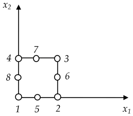
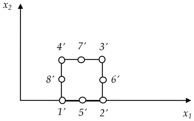
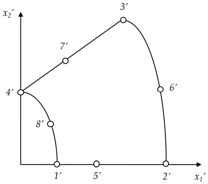
where $A$ and $B$ are complex numbers. This transformation is a combination of translation, rotation, and stretching. It is easy to verify by looking at the derived stiffness matrix for a single element that under this transformation, the stiffness matrix is invariant. We illustrate this computationally for the unit eight-node quadratic element in the plane $x_1{x}_2$ displayed in Figure 1. By taking $A=2e^{i{\displaystyle \frac{\pi }{4}}}$ and $B=1+2i$, the coordinates transform as

$${x^{\prime }}_1=\sqrt{2}{x}_1-\sqrt{2}{x}_2+1 \mathrm{and} {x^{\prime }}_2=\sqrt{2}{x}_1+\sqrt{2}{x}_2+2$$

(66a,b)

The stiffness matrix for both cases is identical.

Table 1. Stiffness matrix for the unit square and for mapped domains under linear and quadratic transformations.

1.15556
0.50000	1.15556
0.51111	0.50000	1.15556
0.50000	0.51111	0.50000	1.15556
−0.82222	−0.82222	−0.51111	−0.51111	2.31111
−0.51111	−0.82222	−0.82222	−0.51111	0.00000	2.31111
−0.51111	−0.51111	−0.82222	−0.82222	0.35556	0.00000	2.31111
−0.82222	−0.51111	−0.51111	−0.82222	0.00000	0.35556	0.00000	2.31111

provides the individual matrix entries, which are exactly the same to six digits from both the research Matlab FE code and ABAQUS 2025 [29].

6.2. Example 2

Now, let us consider the mapping defined by

$$z^{\prime }=\Omega \left(z\right)=z^2$$

(67)

In this case, for the mapped coordinates, we have

$$x_1^{\prime }=x_1^2-x_2^2 \mathrm{and} x_2^{\prime }=2x_1{x}_2$$

(68a,b)

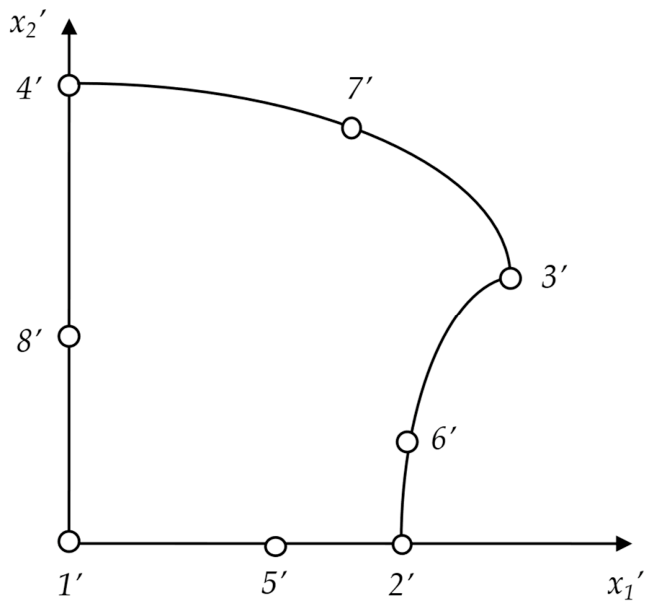
Consider the unit serendipity quadratic element in the plane $x_1{x}_2$ displayed in Figure 2. This element is exactly the element in Figure 1, which has been translated in the $x_1$-direction by a unit amount. The mapped element in the plane $x_1^{\prime }{x}_2^{\prime }$ is shown in Figure 3. It is seen that the side mid-nodes have shifted from the center of the edge in this transformation. The stiffness matrix for both cases is again identical, as indicated in Table 1. The quadratic transformation can be accommodated exactly with the quadratic shape functions used to describe the element geometry.

6.3. Example 3

Now, let us consider the mapping defined by

$$z^{\prime }=\Omega \left(z\right)=\sin \left(z\right)$$

(69)

In this case, the mapped coordinates are

$$x_1^{\prime }=\sin \left(x_1\right)\cosh \left(x_2\right) \mathrm{and} x_2^{\prime }=\cos \left(x_1\right)\sinh \left(x_2\right)$$

(70a,b)

We again focus on the unit quadratic element in the plane $x_1{x}_2$ displayed in Figure 1. For this example, the mapped element in the plane $x_1^{\prime }{x}_2^{\prime }$ is displayed in Figure 4. The stiffness matrix for the mapped element is given in

Table 2. Stiffness matrix for the mapped domain of the unit square under $z^{\prime }=\sin \left(z\right)$.

1.14332
0.48279	1.15172
0.50954	0.51169	1.1629
0.50637	0.50922	0.49043	1.15480
−0.78531	−0.79240	−0.51629	−0.51097	2.24611
−0.50435	−0.84911	−0.85800	−0.51002	−0.00089	2.38543
−0.49249	−0.49484	−0.77705	−0.77147	0.35303	−0.01505	2.20406
−0.85987	−0.51906	−0.52318	−0.86837	0.00672	0.35199	−0.00618	2.41795

, which differs slightly from the stiffness matrix of the unit square element provided in Table 1. The difference is the result of using quadratic shape functions for defining the geometry in the mapped domain. Numerical integration also plays a role.

Thus, in this case, a single element cannot precisely accommodate the mappings as required to preserve the invariant nature of the stiffness matrix. However, with mesh refinement, the stiffness matrix $K$ and therefore the condensed boundary stiffness matrix ${\overline{K}}_{BB}$ will tend toward invariance.

Table 3. Principal stiffnesses for the individual elements of the mapped domain within the unit square under $z^{\prime }=\sin \left(z\right)$.

Mode $\mathit{i}$	Principal Stiffnesses ${\mathit{\lambda }}_{{\mathit{K}}_{\mathit{i}}}$	Square $1\times 1$ Mesh	Mapped Domain $1\times 1$ Mesh	Error Mapped Domain $1\times 1$ Mesh	Error Mapped Domain $2\times 2$ Mesh	Error Mapped Domain $4\times 4$ Mesh	Error Mapped Domain $16\times 16$ Mesh
1	0.000000	0.000000	0.000000	-	-	-	-
2	0.510485	0.510485	0.508005	0.0049	0.0008	0.0002	1.3 × 10−5
3	0.510485	0.510485	0.511653	0.0023	0.0009	0.0002	1.5 × 10−5
4	0.666667	0.666667	0.666917	0.0004	4.7 × 10−5	1.3 × 10−6	<1.0 × 10−6
5	2.089515	2.089515	1.984975	0.0527	0.0133	0.0033	0.0002
6	2.089515	2.089515	2.204007	0.0519	0.0133	0.0033	0.0002
7	2.666667	2.666667	2.667933	0.0005	8.0 × 10−5	1.8 × 10−6	<1.0 × 10−6
8	5.333333	5.333333	5.322762	0.0020	0.0004	3.7 × 10−6	<1.0 × 10−6

presents the eight principal stiffnesses (or eigenvalues) of the stiffness matrix associated with an 8-noded element representing the unit square. The second column provides the exact values of these principal stiffnesses, while the third column shows those values for the element in the original $x_1{x}_2$ domain. Notice that there is one zero principal stiffness associated with the equipotential mode. The fourth column presents the computed principal stiffnesses in the $x_1^{\prime }{x}_2^{\prime }$ domain under the $z^{\prime }=\sin \left(z\right)$ mapping. The error in those values is shown in the fifth column. Modes five and six have more than $5\%$ error. Next, the mesh used for the unit square is refined to $2\times 2$, $4\times 4$ and $16\times 16$ elements. The errors associated with the lowest eight principal stiffnesses are provided in the last three columns. Clearly, the character of the stiffness matrices is converging toward invariance. In the finest mesh, the maximum error is only $0.02\%$.

6.4. Example 4

As we mentioned previously, the unit circular disc has great importance in conformal mapping methods for solving boundary value problems. Additionally, the normalized fundamental boundary eigensolutions for a circular disc with radius $a$ and $\varphi =1$ on the boundary are provided in closed form in Equations (42)–(44).

Consider the conformal mapping of the unit disc under the transformation

$$z^{\prime }=\Omega \left(z\right)=e^{\sin \left(z\right)}$$

(71)

The mapped coordinates are

$$x_1^{\prime }=e^{\sin \left(x_1\right)\cosh \left(x_2\right)}\cos \left[\cos \left(x_1\right)\sinh \left(x_2\right)\right]$$

(72a)

$$x_1^{\prime }=e^{\sin \left(x_1\right)\cosh \left(x_2\right)}\sin \left[\cos \left(x_1\right)\sinh \left(x_2\right)\right]$$

(72b)

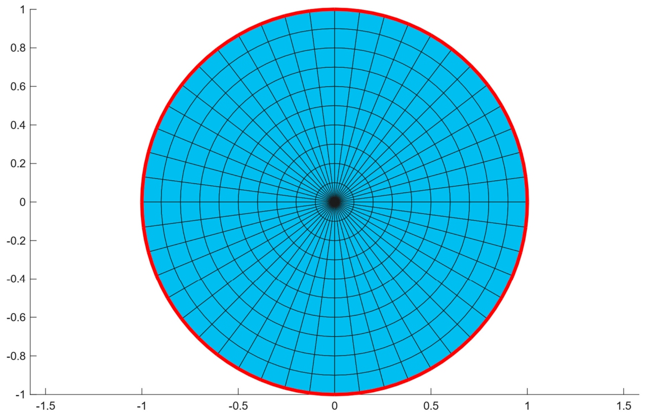
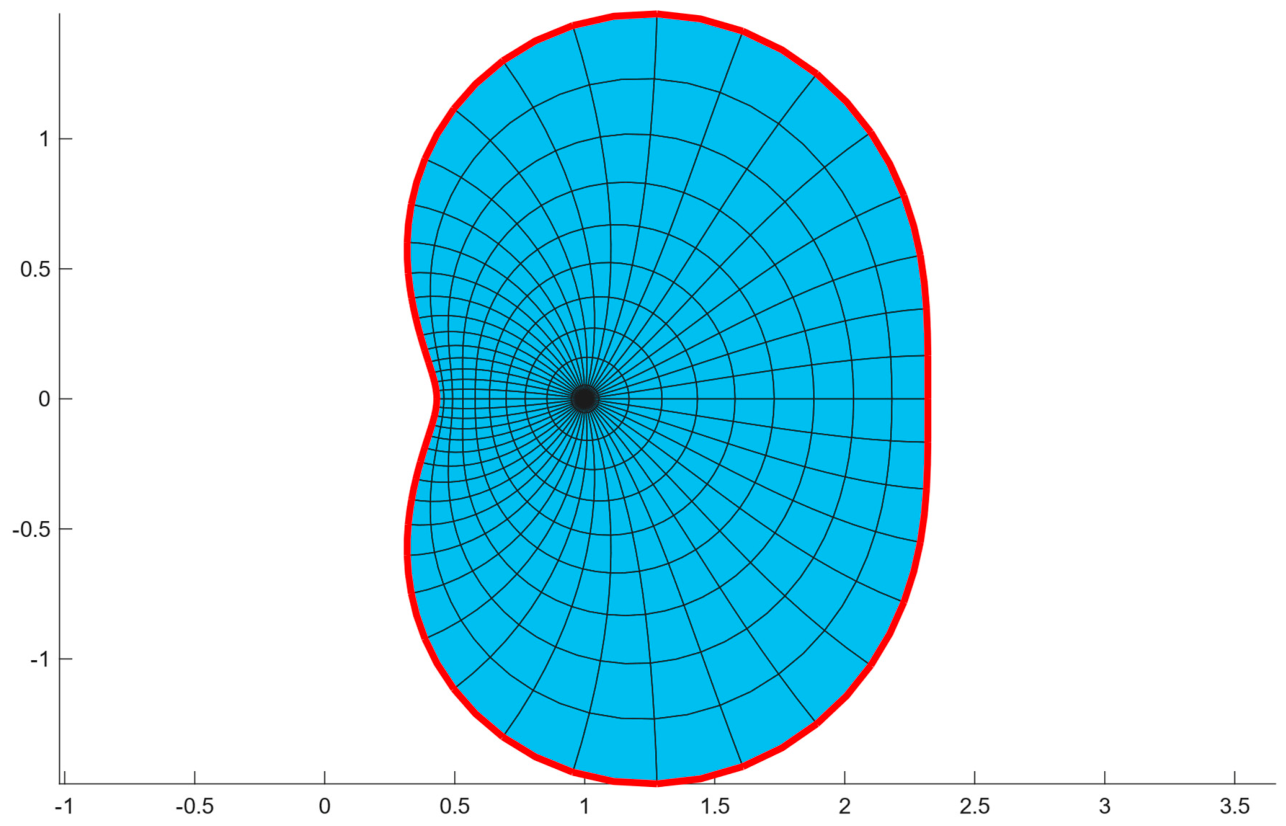
Figure 5 provides the finite element mesh used for discretizing the unit disc. The mesh involves a total of 480 serendipity quadratic elements and 1441 nodes. A total of 48 six-node triangular elements are employed for the innermost region connecting to the node at $z=0$. Meanwhile, the mapped FE discretization is shown in Figure 6. Interestingly, the mapped configuration of the unit disc resembles a Pascal’s limaçon-like shape. It is evident that the circular symmetry is not preserved in the mapped mesh.

The corresponding boundary mesh on the circle consists of 48 equal-length quadratic elements and 96 equispaced nodes for calculating the ${\widehat{S}}^{\varphi }$ matrix. We know the number of approximated boundary eigensolutions is equal to the number of boundary nodes (i.e., 96). By choosing

$${\varphi }^{\prime }=\left|{\displaystyle \frac{d{z}^{\prime }}{dz}}\right|=\left|\cos z\right|\left|e^{\sin \left(z\right)}\right|$$

(73)

we expect the eigensolutions for the mapped domain to be similar to those for the circular disc. This is shown in

Table 4. Eigenvalues for the circular disc and its mapped domain under $z^{\prime }=e^{\sin \left(z\right)}$.

Mode	Exact	FE (Original)	FE (Mapped)	BE (Original)	BE (Mapped)
2	1.0000	1.0000	1.0000	1.00000	0.99996
4	2.0000	2.0000	2.0000	2.0000	2.0000
8	4.0000	4.0002	4.0002	4.0003	4.0001
12	6.0000	6.0018	6.0017	6.0021	6.0013
18	9.0000	9.0149	9.0149	9.0145	9.0133
25	12.000	12.069	12.070	12.055	12.056
30	15.0000	15.240	15.240	15.150	15.147
40	20.0000	21.311	21.310	20.444	20.439
50	25.0000	30.684	30.668	28.495	28.471
60	30.0000	44.389	44.389	34.546	34.536
70	35.0000	64.433	64.433	42.270	42.266
80	40.0000	90.183	90.181	49.945	49.917
95	47.0000	118.38	118.50	56.175	56.182
96	48.0000	118.97	119.10	107.51	56.295

. As we can see, excellent results are obtained for lower modes in both the original and mapped FE analysis. The results deteriorate for higher modes; however, the eigenvalues are nearly identical from both FE analyses. Thus, the discrete version of the boundary eigenproblem remains nearly invariant under the transformation defined by Equation (71).

We also include the boundary element (BE) results with quadratic elements for the original and mapped meshes in Table 4. Although neither system matrix in BE remains invariant under the mapping, we find that the BE results for both domains are more accurate than the FE results. This is particularly true for higher modes due to the use of the exact fundamental solution to the potential problem in the interior of the domain in the BE formulation, whereas a finite discretization of the interior is employed in the FE analysis.

As we have proved, ${\overline{K}}_{BB}$ and ${\widehat{S}}^{\varphi }$ for both meshes should be the same, at least in the limit of mesh refinement. For the present models, these matrices are $96\times 96$.

Table 5. ${\overline{K}}_{BB}$ for the unit disc in example 4.

1.35200
−0.638755	1.83540
0.056279	−0.638755	1.35200
−0.0181344	−0.133685	−0.638754	1.835401
−0.0295271	−0.0181344	0.0562790	−0.638755	1.352002

and

Table 6. ${\widehat{S}}^{\varphi }$ for the unit disc in example 4.

0.034930
0.0087284	0.069785
−0.0043642	0.0087284	0.034930
0.00000	0.00000	0.0087284	0.069785
0.00000	0.00000	−0.0043642	0.0087285	0.034930

show the characteristic $5\times 5$ diagonal block of these matrices for the circular disc. Cyclic symmetry of the numbers is obviously maintained throughout the entire matrices because of the cyclic symmetry of the mesh.

Table 7. ${\overline{K}}_{BB}$ for the unit disc under $\Omega \left(z\right)=e^{\sin \left(z\right)}$ in example 4.

1.35410
−0.64176	1.84202
0.057767	−0.640680	1.35393
−0.017917	−0.134228	−0.64221	1.840717
−0.029503	−0.0181419	0.057444	−0.639348	1.35345

and

Table 8. ${\widehat{S}}^{\varphi }$ for the unit disc under $\Omega \left(z\right)=e^{\sin \left(z\right)}$ in example 4.

0.034787
0.0087180	0.069959
−0.0043589	0.0087178	0.034806
0.00000	0.00000	0.0087206	0.069914
0.00000	0.00000	−0.0043600	0.0087194	0.034854

represent the same parts for the mapped mesh. As anticipated, the values in the matrices are quite similar to the corresponding ones in Table 5 and Table 6. The differences are again due to the inability of the quadratic shape function to provide an exact map of the conformal transformation. In the limit of mesh refinement, we should expect the invariance of ${\overline{K}}_{BB}$ and ${\widehat{S}}^{\varphi }$ to be realized.

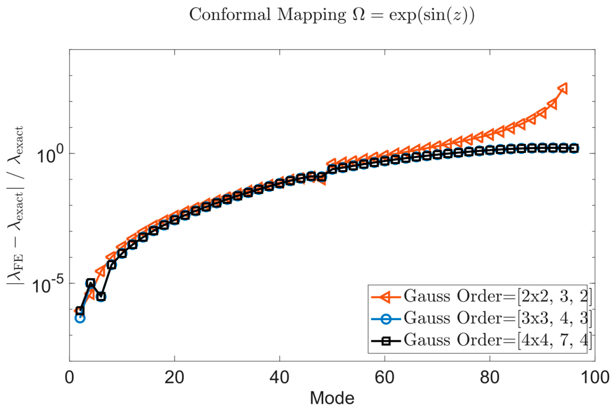
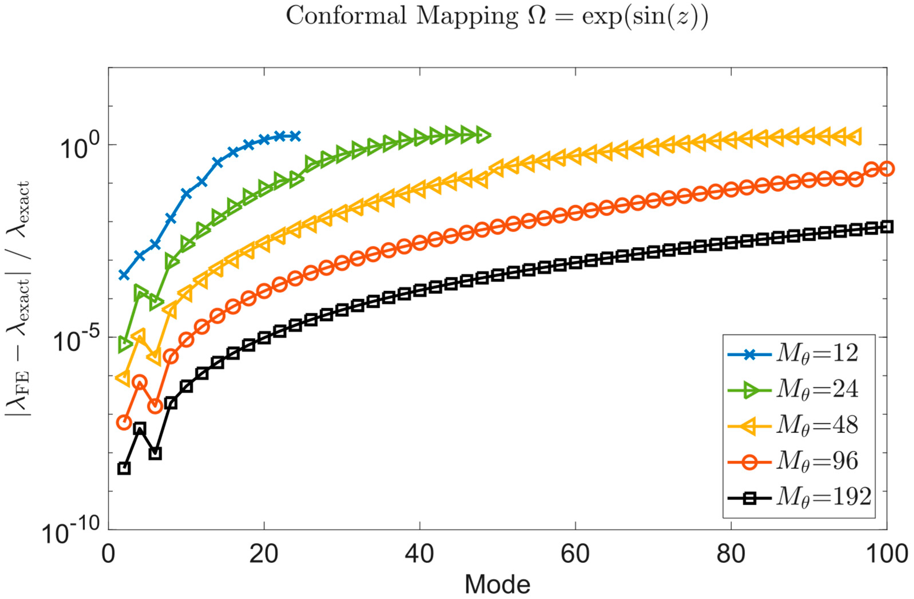
Figure 7 provides the convergence characteristics of the eigenvalues for various numbers of elements $M_{\theta }$ around the circumference of the circle (or perimeter of the mapped domain). Meanwhile, the number of elements in the radial direction $M_r$ is varied to maintain a nearly constant ratio $M_{\theta }/M_r\approx 4.8$. The semi-log plot in Figure 7 presents relative errors in the eigenvalues versus mode number. Clearly, accuracy improves with FE mesh refinement and deteriorates for higher modes. The oscillation at lower modes and the jump at the midrange mode are artefacts of the use of quadratic elements, which have different ${\overline{K}}_{BB}$ and ${\widehat{S}}^{\varphi }$ values associated with the corner and mid-nodes, as seen in Table 5, Table 6, Table 7 and Table 8. 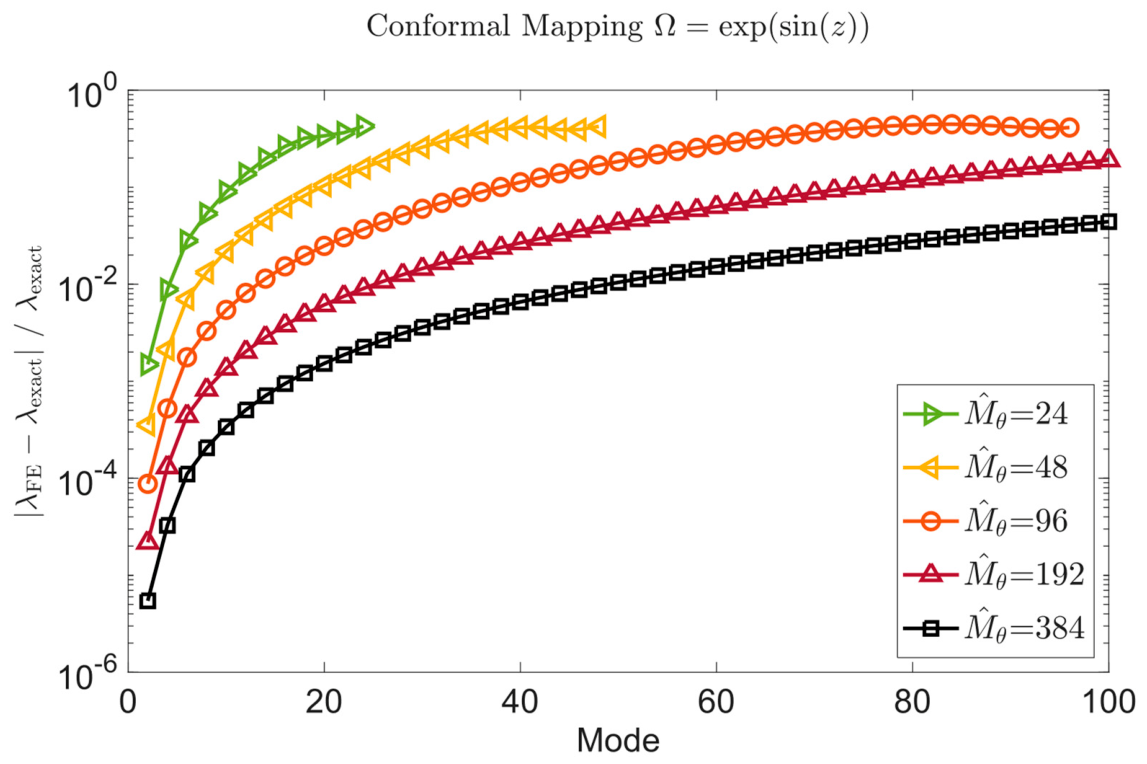Figure 8 provides the corresponding results using linear elements, where now ${\widehat{M}}_{\theta }$ represents the number of linear elements around the circumference of the circle. Notice that there are no oscillations or jumps of the errors in the eigenvalues with linear elements, although the levels of error are greater, as would be expected.

Integration order also plays a role, especially for lower and higher modes, as shown in Figure 9. The Gaussian quadrature order is defined by $[n_q\times n_q, n_t, n_s]$ with $n_q$, $n_t$ and $n_s$ representing the quadrilateral, triangular, and surface element integration orders, respectively. The oscillation in the lower mode accuracy disappears when using low-order integration, at the expense of loss of accuracy for higher modes. There is almost no difference between the intermediate and highest order integration solutions.

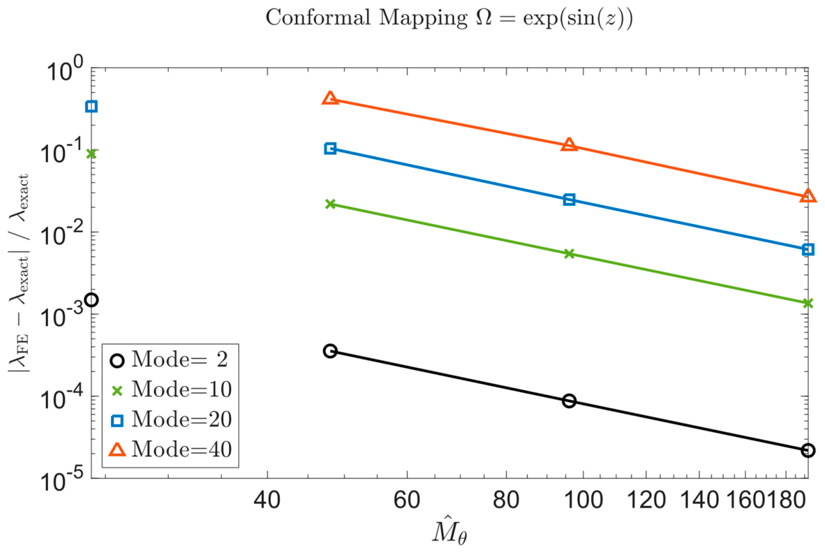
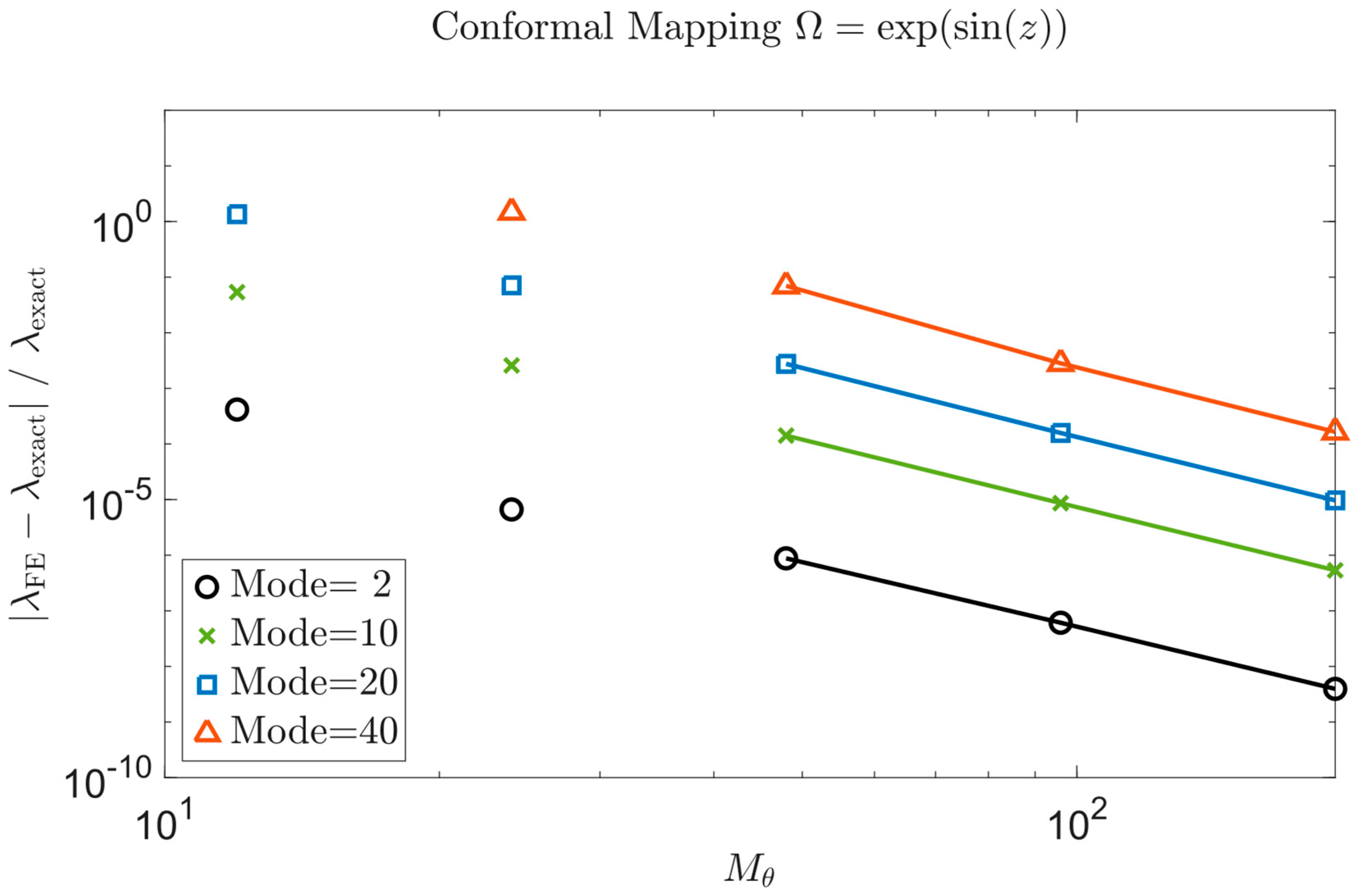
Lastly, for this problem, the rate of convergence of the second, tenth, twentieth, and fortieth modes is presented in Figure 10. Accuracy deteriorates with increasing mode number, as expected. However, the rate of convergence remains nearly the same, with slopes from the log-log plot of $-3.75$, $-4.02$, $-4.08$ and $-4.36$ for Modes $2$, $10$, $20$ and $40$, respectively. This corresponds to roughly quadratic convergence of the eigenvalues with respect to the total FE degrees of freedom in the domain. The corresponding results for linear elements are provided in Figure 11. The slopes of the log-log plot are now $-2.01$, $-2.01$, $-2.04$ and $-1.98$ for Modes $2$, $10$, $20$ and $40$, respectively. Thus, linear elements display a linear rate of convergence with total degrees of freedom, as would be anticipated.

6.5. Example 5

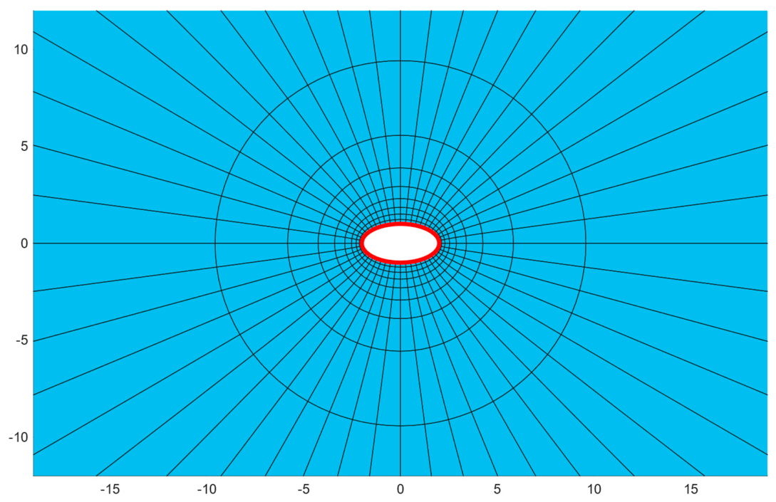
Now we use the stiffness matrix for the circular disc in Example 4 with quadratic elements to analyze an infinite domain with an elliptic hole. The transformation

$$z^{\prime }=\Omega \left(z\right)=\alpha z+{\displaystyle \frac{\beta }{z}}$$

(74)

with

$$\alpha ={\displaystyle \frac{a+b}{2}} \mathrm{and} \beta ={\displaystyle \frac{a-b}{2}}$$

(75a,b)

transforms the interior of the unit disc in the $x_1{x}_2$-plane to the exterior of the ellipse with semi-axes $a$ and $b$ on the plane $x_1^{\prime }{x}_2^{\prime }$. The mapped coordinates are

$$x_1^{\prime }=\left(\alpha r+{\displaystyle \frac{\beta }{r}}\right)\cos \theta$$

(76a)

$$x_2^{\prime }=\left(\alpha r-{\displaystyle \frac{\beta }{r}}\right)\sin \theta$$

(76b)

and for boundary points are

$$x_1^{\prime }=a{x}_1$$

(77a)

$$x_2^{\prime }=b{x}_2$$

(77b)

For this example, we assume $a=2$ and $b=1$. Therefore,

$$z^{\prime }={\displaystyle \frac{3}{2}}z+{\displaystyle \frac{1}{2z}}$$

(78)

We again consider the finite element mesh used for discretizing the unit disc in Figure 5. The mapped FE discretization for boundary nodes is shown in Figure 12. For the weight function in this example, we assume

$${\varphi }^{\prime }=\varphi =1$$

(79)

Therefore, ${\widehat{S}}^{\varphi }$ is not invariant, and neither are the boundary eigensolutions. In this example, we are simply trying to demonstrate that ${\overline{K}}_{BB}$ for an internal unit, a disc can be used directly for external problems.

Figure 12. Transformation of the unit disc under $\Omega \left(z\right)={\displaystyle \frac{3}{2}}z+{\displaystyle \frac{1}{2z}}$—boundary nodes of circle and ellipse.

Figure 12. Transformation of the unit disc under $\Omega \left(z\right)={\displaystyle \frac{3}{2}}z+{\displaystyle \frac{1}{2z}}$—boundary nodes of circle and ellipse.

Table 9. Eigenvalues for infinite domain with elliptical hole in example 5.

Mode	FE	BE
2	0.55503	0.55504
4	1.2515	1.2516
8	2.5793	2.5795
12	3.8880	3.8885
18	5.8514	5.8495
25	7.8563	7.8334
30	9.9837	9.8512
40	14.009	13.044
50	20.158	17.575
60	29.424	22.075
70	42.644	27.150
80	57.754	31.509
95	109.559	53.424
96	109.559	53.424

compares the boundary eigenvalues for the external ellipse eigenproblem from the conformally mapped FE analysis with the exterior ellipse boundary element (BE) results. Excellent agreement is obtained for the lower modes. In general, we can expect that the BE results are more accurate than the mapped FE results, particularly for higher modes. This is because, as mentioned, in a boundary element formulation, the volume integrals are transformed analytically to the boundary using the infinite space fundamental solution, along with the divergence theorem, whereas in this flux-oriented finite element method, the transformation is performed numerically via condensation. It should be mentioned that $S^{\varphi }$ can be a rectangular matrix to permit discontinuity in the weighted traction vector $Q^{\varphi }$. However, the important point is that these infinite domain FE results are determined by using the stiffness matrix for the interior of a unit circular disc. Consequently, we have demonstrated an elegantly simple way to use the finite element method for an infinite two-dimensional domain.

6.6. Example 6

Finally, we use the stiffness matrix for the circular disc in Examples 4 and 5 based on $M_{\theta }=48$ and $M_r=10$ quadratic elements to analyze an external boundary value problem. Our example is a cracked infinite plate under anti-plane deformation. This problem has an analytical solution that can be found in Benthem and Koiter [30]. In the following, we use a slightly different form.

The anti-plane problem is characterized by a single displacement component $u\left(x_1,x_2\right)$ normal to the plane $x_1{x}_2$. The non-vanishing stress components are the shear stresses ${\sigma }_{31}={\tau }_1$ and ${\sigma }_{32}={\tau }_2$ in the plane $x_1{x}_2$ given by

$${\tau }_1=\mu {\displaystyle \frac{\partial u}{\partial x_1}}$$

(80a)

$${\tau }_2=\mu {\displaystyle \frac{\partial u}{\partial x_2}}$$

(80b)

where $\mu$ is the shear modulus of elasticity. From equilibrium $u$ is a harmonic function, and the anti-plane state of stress is described by a single analytic function $w\left(z\right)$ as

$$u\left(x_1,x_2\right)=\Re \left[w\left(z\right)\right]$$

(81a)

where we have

$${\tau }_1-i{\tau }_2=\mu {\displaystyle \frac{dw}{dz}}$$

(81b)

If in the transformation Equation (74), we consider

$$\alpha =\beta ={\displaystyle \frac{a}{2}}$$

(82)

we obtain

$$z^{\prime }=\Omega \left(z\right)={\displaystyle \frac{a}{2}}\left(z+{\displaystyle \frac{1}{z}}\right)$$

(83)

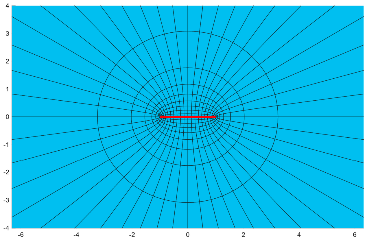
where $2a$ is the length of the central crack in the $x_1{x}_2$-plane. This transformation maps the interior of the unit circular disc in the $x_1{x}_2$-plane to the whole plane $x_1^{\prime }{x}_2^{\prime }$ with the crack that extends from $x_1^{\prime }=-a$ to $x_1^{\prime }=a$ on $x_2^{\prime }=0$. From

$${\displaystyle \frac{d{z}^{\prime }}{dz}}={\displaystyle \frac{d\Omega \left(z\right)}{dz}}={\displaystyle \frac{a}{2}}\left(1-{\displaystyle \frac{1}{z^2}}\right)$$

(84)

it is seen that the points $z=\pm 1$ are critical points of the transformation. This allows us to have crack tips at $z^{\prime }=\pm a$ in the mapped domain. The transformation relates the crack coordinates in terms of the unit circle boundary as

$$x_1^{\prime }=a{x}_1=a\cos \theta$$

(85a)

$$x_1^{\prime }=0$$

(85b)

The mapped FE discretization for boundary nodes is shown in Figure 13. To solve the problem of the crack loaded uniformly at infinity, we may consider the superposition of two cases. The first involves the infinite plane under uniform shear stress $-T_0$, while for the second case, we apply a uniform shear on the crack

$${\tau }_2^{\prime }=T_0\hspace{1em}\hspace{1em}\mathrm{on} -a\le x_1^{\prime }\le a,\hspace{1em}\hspace{1em}{x}_2^{\prime }=0$$

(86)

with zero shear at infinity. The solution to the first case is obvious. For the second case, we have

$$\mu w^{\prime }\left(z^{\prime }\right)=i{T}_0{z}^{\prime }-i{T}_0\sqrt{{z^{\prime }}^2-a^2}$$

(87a)

As a result,

$${\tau }_2^{\prime }+i{\tau }_1^{\prime }=i\mu {\displaystyle \frac{d{w}^{\prime }\left(z^{\prime }\right)}{d{z}^{\prime }}}=-T_0+T_0{\displaystyle \frac{z^{\prime }}{\sqrt{{z^{\prime }}^2-a^2}}}$$

(87b)

Therefore, on the line $x_2^{\prime }=0$,

$${\left.\mu w^{\prime }\right|}_{x_2^{\prime }=0}=i{T}_0{x}_1^{\prime }-i{T}_0\sqrt{{x_1^{\prime }}^2-a^2}$$

(88a)

$${\left.{\tau }_2^{\prime }+i{\tau }_1^{\prime }\right|}_{x_2^{\prime }=0}=-T_0+T_0{\displaystyle \frac{x_1^{\prime }}{\sqrt{{x_1^{\prime }}^2-a^2}}}$$

(88b)

Furthermore,

$$u^{\prime }\left(x_1^{\prime },0^{+}\right)=\left\{\begin{array}{c}{\displaystyle \frac{T_0}{\mu }}\sqrt{a^2-{x_1^{\prime }}^2}\hspace{1em}\hspace{1em}\left|x_1^{\prime }\right|\le a\\ 0\hspace{1em}\hspace{1em}\hspace{1em}\hspace{1em}\hspace{1em}\hspace{1em} \left|x_1^{\prime }\right|>a\end{array}\right.$$

(89)

and

$${\tau }_2^{\prime }\left(x_1^{\prime },0^{+}\right)=\mu {\displaystyle \frac{d{u}^{\prime }\left(x_1^{\prime },0^{+}\right)}{d{x}_2^{\prime }}}=\left\{\begin{array}{c}-T_0\hspace{1em}\hspace{1em}\hspace{1em}\hspace{1em}\hspace{1em}\hspace{1em}\hspace{1em}\hspace{1em}\hspace{1em} \left|x_1^{\prime }\right|\le a\\ -T_0+T_0{\displaystyle \frac{x_1^{\prime }}{\sqrt{{x_1^{\prime }}^2-a^2}}}\hspace{1em}\hspace{1em}\hspace{1em}\hspace{1em}\left|x_1^{\prime }\right|>a\end{array}\right.$$

(90)

In addition, we notice that

$$u^{\prime }\left(x_1^{\prime },0^{-}\right)=-u^{\prime }\left(x_1^{\prime },0^{+}\right),{\displaystyle \frac{d{u}^{\prime }\left(x_1^{\prime },0^{-}\right)}{d{x}_2^{\prime }}}=-{\displaystyle \frac{d{u}^{\prime }\left(x_1^{\prime },0^{+}\right)}{d{x}_2^{\prime }}}$$

(91a,b)

Consequently,

$$\tau ={\tau }_2^{\prime }\left(x_1^{\prime },0\right)=-T_0+T_0{\displaystyle \frac{x_1^{\prime }}{\sqrt{{x^{\prime }}_1^2-a^2}}}\hspace{1em}\hspace{1em}\hspace{1em}\left|x_1^{\prime }\right|>a$$

(92)

which shows, of course, that the stresses are infinite at the crack tips. By assuming $\xi =x_1^{\prime }-a$ where $x_1^{\prime }>a$, it is seen that

$${\tau }_2^{\prime }\left(\xi \right)=-T_0+T_0{\displaystyle \frac{a+\xi }{\sqrt{\xi \left(2a+\xi \right)}}}=T_0\sqrt{{\displaystyle \frac{a}{2\xi }}}\hspace{1em}\hspace{1em}\hspace{1em}\left|x_1^{\prime }\right|>a$$

(93)

By definition, the tearing stress intensity factor (Mode III) in fracture mechanics is

$$K_{III}=\underset{\xi \to 0}{\lim }\sqrt{2\pi \xi }{\tau }_2^{\prime }\left(\xi \right)$$

(94)

As a result, Equation (93) shows that

$$K_{III}=T_0\sqrt{\pi a}$$

(95)

Next, we solve this problem using the finite element method. We assume $\mu =1$, $a=1$ and $T_0=1$ for the computational test. We have a Neumann problem for the cracked infinite domain with a traction boundary condition

$$t_2^{\prime }=T_0\hspace{1em}\mathrm{on} -a\le x_1^{\prime }\le a, x_2^{\prime }=0^{+} \mathrm{upper} \mathrm{crack} \mathrm{surface}$$

(96a)

$$t_1^{\prime }=-T_0\hspace{1em}\mathrm{on} -a\le x_1^{\prime }\le a, x_2^{\prime }=0^{-} \mathrm{lower} \mathrm{crack} \mathrm{surface}$$

(96b)

It is seen that the equilibrium on the crack surfaces

$${\displaystyle {\displaystyle \underset{-a}{\overset{a}{\int }}}{t}_2^{\prime }\left(x_1^{\prime },0^{+}\right)d{x}_1}+{\displaystyle {\displaystyle \underset{-a}{\overset{a}{\int }}}{t}_2^{\prime }\left(x_1^{\prime },0^{-}\right)d{x}_1}=0$$

(97)

is satisfied. This guarantees that the stress is zero at infinity, and we can use

$$KU=\left\{\begin{array}{c}{S}^{\prime }{Q}^{\prime }\\ 0\end{array}\right\}$$

(98)

or

$${\overline{K}}_{BB}{U}_B=S^{\prime }{Q}^{\prime }$$

(99)

in which $K$ and ${\overline{K}}_{BB}$ are the global stiffness matrix and the condensed boundary stiffness matrix for the interior unit circular disc, respectively. Meanwhile, $S^{\prime }$ is the boundary matrix for the cracked boundary, in which we assume ${\mathbf{\varphi }}^{\prime }=1$. It should be mentioned that the mapped boundary elements are not of uniform length, and the mid-nodes are no longer at the element center. Alternatively, we could calculate $S^{\prime }$ from the original boundary nodes on the unit circle, as long as we choose

$$\varphi \left(x\right)=\sqrt{J\left(x\right)}=a{x}_2=a\left|\sin \theta \right|$$

(100)

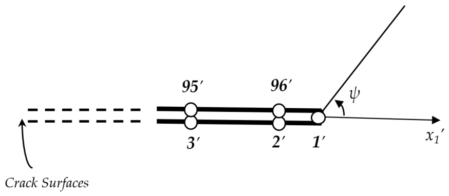
To suppress the rigid body motion for this Neumann problem, we have utilized a singular value decomposition [31]. As a result, the first node at the right crack tip has zero displacements. Then, the computational results for $u^{\prime }$ are very accurate on the crack. By using local analysis near the right crack tip, as shown in Figure 14, we obtain

$$u^{\prime }\left(\rho ,\psi \right)=-{\displaystyle \frac{T_0}{\mu }}\rho \sin \left(\psi \right)+C_1{\rho }^{{\displaystyle \frac{1}{2}}}\sin \left({\displaystyle \frac{\psi }{2}}\right)+C_3{\rho }^{{\displaystyle \frac{3}{2}}}\sin \left({\displaystyle \frac{3\psi }{2}}\right)+\cdots$$

(101)

It is seen that

$$C_1={\displaystyle \frac{1}{\mu }}\sqrt{{\displaystyle \frac{2}{\pi }}}{K}_{III}$$

(102)

Therefore, we have on the upper crack surface ($\psi =\pi$) near the crack tip

$$u^{\prime }\left(\rho ,\psi =\pi \right)={\displaystyle \frac{1}{\mu }}{K}_{III}\sqrt{{\displaystyle \frac{2\rho }{\pi }}}$$

(103)

From the finite element solution using the unit circular disc mesh in the $x_1{x}_2$-plane with $\varphi =a{x}_2$, we find for the node 2 adjacent to the crack tip at node 1

$$\rho =0.002141, u=0.065403$$

(104)

and the tearing stress intensity factor becomes

$$K_{III}=\mu \sqrt{{\displaystyle \frac{\pi }{2\rho }}}{u}^{\prime }\approx 1.7715$$

(105)

Meanwhile, the exact value for $K_{III}$ from Equation (94) is

$${\left.K_{III}\right|}_{\mathrm{exact}}=\sqrt{\pi }\approx 1.7724$$

(106)

Therefore, we see that a very precise evaluation of the stress intensity factor can be obtained by using the finite element stiffness matrix for the interior of a unit circular disc.

It should be mentioned that the positions of mapped nodes on the crack boundary are crucial in obtaining results with this level of accuracy. The crack nodes are positioned on the axis $x_1^{\prime }$ with the arrangement of

$$x_{1\left(m\right)}^{\prime }=a\cos \left[\left(m-1\right)\Delta \theta \right]$$

(107)

where the node number $m=1,2,\cdots ,N$, $\Delta \theta ={\displaystyle \frac{2\pi }{N}}$, and $N=96$ is the total number of nodes. Clearly, this arrangement of nodes is not uniform. For the nodes near the right crack tip in Figure 14, it is seen that $x_{1\left(1\right)}^{\prime }=a$, $x_{1\left(2\right)}^{\prime }=x_{1\left(96\right)}^{\prime }=a\left[1-{\displaystyle \frac{1}{2}}\Delta {\theta }^2\right]$ and $x_{1\left(3\right)}^{\prime }=x_{1\left(95\right)}^{\prime }=a\left[1-2\Delta {\theta }^2\right]$. This means for near crack tip elements, the middle node in quadratic elements moves to almost the quarter point. Of course, quarter-point elements are well-known in the analysis of cracked bodies [32,33]. With the present approach, all nodes on the unit circle change position on crack surfaces to provide an amazingly accurate result. Exactly the same behavior occurs near the left crack tip.

As noted above, singular value decomposition was used to eliminate rigid body motion. The other way to suppress rigid body motion is to modify the global stiffness matrix $K$ such that the node at the center of the circular disc is fixed. In the mapped domain, this corresponds to fixing the stiffness at infinity, because the point $z=0$ maps to $z^{\prime }=\infty$, which is assumed to be fixed. After condensing for boundary nodes, we obtain the modified condensed boundary stiffness matrix, which is non-singular. We can obtain exactly the same results as before without fixing any node on the crack using either of Equation (98) or (99).

Table 10. Tearing stress intensity factors for an infinite plate with a central crack.

${\mathit{M}}_{\mathit{\theta }}$	${\mathit{M}}_{\mathit{r}}$	Circle FE $\begin{array}{c}{\mathit{K}}_{\mathit{I}\mathit{I}\mathit{I}}\\ (\mathit{\varphi }=\mathit{a}{\mathit{x}}_2)\end{array}$	Circle FE Error $\begin{array}{c}{\mathit{K}}_{\mathit{I}\mathit{I}\mathit{I}}\\ (\mathit{\varphi }=\mathit{a}{\mathit{x}}_2)\end{array}$	Mapped FE $\begin{array}{c}{\mathit{K}}_{\mathit{I}\mathit{I}\mathit{I}}\\ ({\mathit{\varphi }}^{\prime }=1)\end{array}$	Mapped FE Error $\begin{array}{c}{\mathit{K}}_{\mathit{I}\mathit{I}\mathit{I}}\\ ({\mathit{\varphi }}^{\prime }=1)\end{array}$
12	3	1.7572	8.634 × 10−3	1.5744	2.433 × 10−1
24	5	1.7687	2.146 × 10−3	1.7788	4.513 × 10−2
48	10	1.7715	5.357 × 10−4	1.7787	2.585 × 10−3
96	20	1.7722	1.339 × 10−4	1.7749	1.272 × 10−3
192	40	1.7724	3.347 × 10−5	1.7734	8.770 × 10−5

displays the convergence characteristics for the tearing stress intensity factors with five levels of mesh refinement, using the two alternative approaches. The first approach employs the original mesh for the circle in the $x_1{x}_2$-plane with $\varphi =a{x}_2$, while the second approach conformally maps the circle to the cracked $x_1^{\prime }{x}_2^{\prime }$ domain with ${\varphi }^{\prime }=1$. Both approaches converge to the exact result $K_{III}=T_0\sqrt{\pi a}$. However, the first approach is slightly more accurate.

6.7. Discussion

We find that the finite element conformal mapping transformation approach employed in these examples demonstrates excellent convergence characteristics toward the exact solutions, confirming the invariance of the stiffness matrix under conformal transformations. In the last problem, the conformal mapping approach is shown to be compatible with two-dimensional anti-plane fracture mechanics analysis. The conformal mapping approach also could be used for other two-dimensional potential problems, such as heat conduction, involving singular fluxes associated with cracks and re-entrant corners. Other advantages of the proposed method include computational economy associated with the reuse of standard well-conditioned meshes, improved accuracy due to invariant internal angles in the transformed finite elements, and a straightforward means to address general non-smooth problems with flux singularities.

7. Conclusions

This paper has shown that the well-established stiffness matrix in potential problems is invariant under a conformal transformation. Consequently, we can calculate the stiffness matrix for a simply connected domain, such as the unit circular disc, and then use it for every simply connected domain (or an infinite domain with a single boundary). The difficulty is finding the corresponding nodes in the new domain, which requires knowledge of the conformal mapping transformation. Furthermore, we can imagine all N-ply connected domains have the same stiffness matrix as long as the conformal mapping functions exist among them.

The weighted boundary matrix ${\widehat{S}}^{\varphi }$ has a significant impact on this subject. It is seen that by choosing a suitable weight function ${\varphi }^{\prime }$, based on the conformal transformation, ${\widehat{S}}^{\varphi }$ also is invariant. This confirms that the fundamental boundary eigensolutions are invariant. As illustrated in the examples, alternative choices for ${\varphi }^{\prime }$ may be appropriate for the effective solution of boundary value problems. In the final example, the conformal mapping approach is applied to calculate the tearing stress intensity factor for a crack in an infinite plate, using the stiffness matrix from the unit circular disc. In all examples, the finite element results are shown to converge to the exact solutions with mesh refinement.

The concepts presented here are primarily of theoretical interest. The invariant character of the stiffness matrix pertains only to conformal transformations within two-dimensional potential problems. However, some of the ideas generated in this work may lead to the development of computational methods with practical utility. For example, one can envision effective finite element approaches for the determination of stress intensity factors (or their generalizations) for cracks, notches, and other non-smooth features that employ the weighted boundary matrix, along with a proper gradation of the mesh in the vicinity of the singularity. Extensions of the approach to permit effective solutions to Helmholtz and transient potential problems would be of great interest, especially those problems with singularities, and are planned for future research. Theoretical advances necessary to consider anisotropic media and three-dimensional models also will be explored.