Bayesian Analysis of Viscous FRW Cosmology with Inhomogeneous Equation of State

Abstract

In this presented work, we execute a statistical data analysis on the viscous models of non-perfect fluid with a viscosity profile $\xi ={\xi }_0+({\xi }_1-{\xi }_{2}q)H$ as well as by taking an equation of state (EOS) characterized by inhomogeneity $p=\omega \rho +\mathsf{\Lambda }\left(t\right)$ and $\omega =\alpha -1$, in the absence of any non-canonical dark energy term with different observational datasets. For the validation of the theoretical study, we carry out Monte Carlo Markov Chain (MCMC) analysis using recent Hubble $H\left(z\right)$, DESI BAO and the Pantheon Plus (PP) datasets to derive the values of constraints. The best-fit results exhibit robust cross-dataset agreement and remain in full agreement with the parameters inferred within the $\mathsf{\Lambda }CDM$ model.

1. Introduction

The accelerated expansion of the late-time universe is explained by introducing dark energy, an ideal cosmic fluid that coexists with ordinary matter and is characterized by a negative pressure and a non-standard EOS. Over the past decades, considerable research has been devoted to understanding the possible mechanisms behind cosmic acceleration, including models based on extended theories of gravity [1,2,3,4,5,6,7,8,9,10] modifications of the equation of state (MEoS). In this context, perfect-fluid models characterized by different equations of state have been widely investigated [11,12,13,14,15,16,17,18,19,20,21,22,23,24] including the Chaplygin gas, generalized Chaplygin gas, barotropic models, and scenarios with inhomogeneous equations of state. However, several of these approaches suffer from hydrodynamic instability. To overcome this drawback, Babichev et al. [25] introduced a more general linear equation of state of the form $p=\beta (\rho -{\rho }_0)$, which, when incorporated into cosmological models, leads to hydrodynamically stable dark energy behavior and provides a consistent description of cosmic acceleration.

Although the perfect-fluid assumption has played a crucial role in understanding the evolution of the universe, particularly during its early hot phases, a more realistic description requires the consideration of imperfect fluids. This is achieved by incorporating viscous effects into cosmological models. Astrophysical observations suggest that the cosmic medium cannot be accurately described as a perfect fluid [26] indicating that viscosity plays an important role in the dynamic evolution of the universe. In particular, bulk viscosity has been investigated from various perspectives [27,28,29] and has proven to be important in building more realistic cosmological models. Moreover, bulk viscosity associated with GUT phase transitions could potentially explain the accelerated expansion of the universe, suggesting that dissipative processes are a fundamental aspect of any realistic cosmological theory.

In recent years, viscous cosmology has gained considerable interest. Brevik et al. [30] showed that, at first order away from equilibrium, the cosmic fluid is characterized by two viscosity coefficients: (i) bulk viscosity $\xi$; and (ii) shear viscosity $\upsilon$. Spatial isotropy justifies neglecting shear viscosity, while fluid-mechanical considerations motivate a linear form for bulk viscosity through its dependence on and the scalar expansion $\theta$. Therefore, the linear combination of ${\xi }_0$ and ${\xi }_1$ has a clearer physical interpretation. This implies that one or more physical quantities diverge and become infinite at a finite future time. It is worth noting that a viscous fluid may also be regarded as a particular case of an inhomogeneous fluid, as originally proposed by Nojiri [17]. The role of bulk viscosity in modifying cosmic pressure and inducing late-time acceleration was investigated by Dou and Meng [31]. They proposed a redshift-dependent cosmological parameter of the form $9\mathsf{\Lambda }={\mathsf{\Lambda }}_0+{\mathsf{\Lambda }}_1{(1+z)}^n$ along with an effective viscous equation of state given by $\xi ={\xi }_0+{\xi }_1{\displaystyle \frac{\dot{a}}{a}}+{\xi }_1{\displaystyle \frac{\ddot{a}}{a}}$. More recently, Normann and Brevik [32] analyzed the key features of two distinct viscous cosmological models. In the first model, dark energy is treated as a single component, with bulk viscosity $\zeta$ arising from the total cosmic fluid and described through a parameterization as $\xi \left(\rho \right)={\xi }_0\left({\displaystyle \frac{\rho }{{\rho }_0}}\right)\mathsf{\Lambda },$ where $\rho$ denotes the dark energy density.

A variety of unified approaches have been proposed to test the plausibility of a single description of the dark sector. These include unified dark fluid (affine) models [33,34,35,36], which assume a single-fluid equation of state. Another class of unification is provided by the Chaplygin gas and generalized Chaplygin gas models [37,38,39] and scalar-field-based approaches [40]. Recent work has also highlighted the role of dark energy in the emergence of cosmic singularities [41]. Furthermore, an ideal fluid model with an inhomogeneous equation of state was proposed in [42].

In modern cosmology, the validity of any theoretical model is assessed through its consistency with observational data. High-precision measurements from cosmic chronometers $H\left(z\right)$, baryon acoustic oscillations (BAOs), and Pantheon Plus provide strong constraints on the expansion history of the universe and the nature of dark energy [43,44,45,46,47]. In this context, cosmological models based on a viscous cosmic fluid and an inhomogeneous equation of state offer a physically motivated framework to describe late-time cosmic acceleration and possible deviations from the standard $\mathsf{\Lambda }CDM$ scenario [48]. Bayesian Markov Chain Monte Carlo (MCMC) analysis is widely used to robustly constrain the free parameters of the given models $Y_1$ and $Y_2$ with present Hubble value $H_0$, which enables an efficient exploration of the parameter space and yields reliable posterior distributions, allowing a statistically consistent comparison between theoretical predictions and observational data [49].

We are motivated by the fact that incorporating an inhomogeneous equation of state enhances the flexibility of the model, allowing a unified description of multiple evolutionary phases of the universe without invoking additional unconventional components. The growing availability of high-precision observational data necessitates robust statistical frameworks such as Bayesian analysis for reliable parameter estimation and model selection, enabling systematic quantification of uncertainties and a consistent assessment of viscous cosmological scenarios. Ultimately, this approach provides a more accurate and physically consistent framework for interpreting observations, constraining dark energy, and guiding the development of extended gravity theories and refined cosmological models. Further, a detailed Bayesian investigation of viscous Friedmann–Robertson–Walker (FRW) cosmology with an inhomogeneous equation of state remains largely unexplored, especially in the context of simultaneously constraining parameters using multiple high-precision observational datasets. Although viscous cosmological frameworks and inhomogeneous equations of state have been examined separately, their unified analysis within a robust Bayesian framework for parameter estimation and model comparison constitutes a novel and significant advancement.

The manuscript is organized as follows. Section 2 discusses the Friedmann-Robertson-Walker (FRW) metric and the corresponding field equations, derives explicit model solutions, and obtains the expression for the Hubble parameter as a function of redshift. Section 3 is devoted to the statistical analysis used to constrain the model parameters with observational data, while Section 4 contains the conclusions and discussion of our findings.

2. Theoretical Framework and Field Equations

We assume a universe which is isotropic as well as homogeneous described by the (FRW) metric [50]

$$d{s}^2=-d{t}^2+{\displaystyle \frac{a^{2}d{r}^2}{1-k{r}^2}}+a^2{r}^2\left(d{\theta }^2+si{n}^2\theta d{\varphi }^2\right)$$

(1)

For a spatially flat universe ($\kappa =0$), the Friedmann equation can be written as [51]

$$3H^2=8\pi G\left(\rho \right),3\dot{H}+3H^2=-4\pi G(\rho +3\overline{p})$$

(2)

Since $\theta =3H$ and $H={\displaystyle \frac{\dot{a}}{a}}$, a is scale factor of the universe which is dependent upon cosmic time t.

The imperfect-fluid energy–momentum tensor introduced by Meng and Ma [52]

$$T_{ij}=\rho u_i+(p-\xi \theta )h_{ij}$$

(3)

where $\rho$ denotes the energy density, pressure is denoted as symbol p, $u_i$ represents the four-velocity component of the cosmic fluid in comoving coordinates, $h_{ij}$ is a tensor representing projection, and the expansion scalar is expressed as $\theta$, where $\xi$ denotes the coefficient of bulk viscosity.

Here we consider the effective pressure $\overline{p}=p-3\xi H$. Substituting in Equation (2) the second Friedmann equation we will get

$$3(\dot{H}+H^2)=-4\pi G(\rho +3p-9\xi H)$$

$$p=\mathsf{\Lambda }\left(t\right)+\omega \rho ,\rho ={\displaystyle \frac{3H^2}{8\pi }}$$

(4)

$$3(\dot{H}+H^2)=-4\pi G\left[{\displaystyle \frac{3H^2(1+3w)}{8\pi G}}+3\mathsf{\Lambda }-9\xi H\right]$$

(5)

For a constant $\omega =\alpha -1$, Equation (2) can be combined to yield

$$\dot{H}=-{\displaystyle \frac{3}{2}}\alpha H^2-4\pi G\mathsf{\Lambda }+12\pi G\xi H$$

(6)

To obtain the solutions of the above equation, we assume that the bulk viscosity depends on the rate of expansion of the universe, and is parameterized as [21]

$$\xi ={\xi }_0+\left({\xi }_1-{\xi }_{2}q\right)H$$

(7)

where ${\xi }_0$, ${\xi }_1$, and ${\xi }_2$ are viscosity constants

$$\dot{H}=-{\displaystyle \frac{3}{2}}\alpha H^2-4\pi G\mathsf{\Lambda }+12\pi G\left[{\xi }_0+\left({\xi }_1-{\xi }_{2}q\right)H\right]H$$

(8)

where the deceleration parameter is denoted and given by [18]

$$q=-{\displaystyle \frac{a\ddot{a}}{{\dot{a}}^2}}=-\left({\displaystyle \frac{\dot{H}+H^2}{H^2}}\right)$$

(9)

$$\dot{H}=-{\displaystyle \frac{3}{2}}\alpha H^2-4\pi G\mathsf{\Lambda }+12\pi G\left[H{\xi }_0+\left({\xi }_1+{\xi }_2\right)H^2+{\xi }_2\dot{H}\right]$$

(10)

$$\left(1-12{\xi }_2\pi G\right)\dot{H}=-{\displaystyle \frac{3}{2}}\alpha H^2-4\pi G\mathsf{\Lambda }+12\pi G\left[H{\xi }_0+\left({\xi }_1+{\xi }_2\right)H^2\right]$$

(11)

The Hubble parameter is expressed in dimensionless form as $h={\displaystyle \frac{H}{H_0}}$ to remove units and simplify the cosmological dynamics. For finding the solution we put cosmological constant $\mathsf{\Lambda }\left(t\right)=\beta h$. Such an assumption is motivated by the idea that the cosmological constant may evolve dynamically with the expansion rate, allowing it to effectively track the Hubble parameter and capture late-time cosmic acceleration within a minimal phenomenological framework. Moreover, such linear dependence ensures dimensional consistency, simplifies the governing equations, and facilitates analytical tractability while retaining the essential coupling between vacuum energy and cosmic expansion.

$$\dot{h}=\left({\displaystyle \frac{-\frac{3}{2}\alpha +12\pi G\left({\xi }_1+{\xi }_2\right)}{1-12{\xi }_2\pi G}}\right)h^2{H}_0+\left({\displaystyle \frac{12\pi G{\xi }_0-\frac{4\pi G\beta }{H_0}}{1-12{\xi }_2\pi G}}\right)h$$

(12)

Equivalently,

$$\dot{h}=P{h}^2{H}_0+Qh$$

(13)

where (P) and (Q) are constants determined by the model parameters. To express the above equation in a more convenient form, we rewrite it in terms of the derivative with respect to $\left(\ln a\right)$, using the relation

$${\displaystyle \frac{d}{dt}}=H{\displaystyle \frac{d}{dlna}}$$

(14)

This leads to

$$h^{\prime }-Ph={\displaystyle \frac{Q}{H_0}}$$

(15)

where the prime denotes differentiation with respect to (ln $a$). This is a first-order linear differential equation, which can be solved using the integrating factor method. The integrating factor is given by

$$\mu \left(a\right)=e^{\int -Pdlna}=a^{-P}$$

(16)

Multiplying the differential equation by the integrating factor, we obtain

$${\displaystyle \frac{d}{dlna}}\left(h{a}^{-P}\right)={\displaystyle \frac{Q}{H_0}}{a}^{-P}$$

(17)

Integrating both sides, we find

$$h,a^{-P}={\displaystyle \frac{Q}{H_0}}\int a^{-P}dlna+C$$

(18)

which gives

$$h\left(a\right)=-{\displaystyle \frac{Q}{P{H}_0}}+C{a}^P.$$

(19)

For convenience, we define the parameters

$$Y_1={\displaystyle \frac{Q}{P{H}_0}},Y_2=-P$$

(20)

so that the solution can be written as

$$h\left(a\right)=Y_1+C{a}^{-Y_2}$$

(21)

The integration constant (C) is determined using the present-time boundary condition $(h\left(a_0\right)=1)$, which yields

$$C=(1-Y_1)a_0^{Y_2}$$

(22)

Substituting this back, the final expression for the dimensionless Hubble parameter becomes

$$h\left(a\right)=(1-Y_1)+Y_1{\left({\displaystyle \frac{a}{a_0}}\right)}^{-Y_2}.$$

(23)

where $\mathcal{P}=\left({\displaystyle \frac{-\frac{3}{2}\alpha +12\pi G\left({\xi }_1+{\xi }_2\right)}{1-12{\xi }_2\pi G}}\right),\mathcal{Q}=\left({\displaystyle \frac{12\pi G{\xi }_0-\frac{4\pi G\beta }{H_0}}{1-12{\xi }_2\pi G}}\right)$

In contrast to $\mathsf{\Lambda }$CDM, the parameters $Y_1$ and $Y_2$ encode the effects of bulk viscosity and an inhomogeneous equation of state, producing a dynamically evolving dark energy component with time-dependent dissipative behavior that departs from equilibrium expansion. The viscous contribution modifies the effective pressure in the Friedmann equations and is carried into the solution through $Y_1$ and $Y_2$, shaping the evolution of $H\left(z\right)$ and introducing entropy production, non-adiabatic effects, and departures from ideal fluid cosmology that can be constrained via Bayesian analysis.

After integration we obtain the corresponding scale factor

$$a\left(t\right)=a_0{\left[{\displaystyle \frac{1}{1-Y_1}}{e}^{(1-Y_1)\left(Y_2\right)H_0(t-t_0)}-{\displaystyle \frac{1}{1-Y_1}}+1\right]}^{{\displaystyle \frac{1}{Y_2}}}$$

(24)

Under this assumption, the Hubble parameter can be determined as a variable of cosmic time t [53]

$$H\left(t\right)=H_0(1-Y_1)\left[{\displaystyle \frac{e^{H_0(Y_1-1)\left(Y_2\right)(t_0-t)}}{e^{H_0(Y_1-1)\left(Y_2\right)(t_0-t)}-Y_1}}\right]$$

(25)

In our model, the bulk viscosity is not introduced explicitly but is effectively encoded through the Hubble function. Since the viscosity depends on the expansion rate, it is indirectly determined by $Y_1$ and $Y_2$. The parameters $Y_1$ and $Y_2$ encode the effective impact of viscosity and the inhomogeneous equation of state on cosmic expansion. Specifically, $Y_1={\displaystyle \frac{Q}{P{H}_0}}$ represents a dimensionless measure of the relative strength of the viscous (or effective dark energy-like) contribution compared to the present Hubble scale, thereby controlling the late-time accelerated expansion and the strength (amplitude) of the viscous effects. The parameter $Y_2=-P$ governs their evolution with redshift and determines the scaling behavior of the dynamical term $a^{-Y_2}$. It is directly linked to the effective pressure term P, which includes bulk viscous effects and governs how viscosity modifies the evolution rate of the Hubble parameter with the scale factor.

Redshift-Dependent Solution for the Viscous Fluid

From Equation (25) we have the Hubble parameter in terms of cosmic time t which can be expressed as

$$w={\displaystyle \frac{Y_{1}H}{H-A}}$$

(26)

where $w=e^{k(t_0-t)},k=A{Y}_2,A=(1-Y_1)H_0$

By applying the logarithm to Equation (26) and differentiating w.r.t z, we obtain the differential equation shown below:

$${\displaystyle \frac{1}{w}}{\displaystyle \frac{dw}{dz}}=\left[{\displaystyle \frac{1}{H}}-{\displaystyle \frac{1}{H-A}}\right]{\displaystyle \frac{dH}{dz}}$$

$${\displaystyle \frac{1}{w}}{\displaystyle \frac{dw}{dt}}{\displaystyle \frac{dt}{dz}}={\displaystyle \frac{-A}{H(H-A)}}{\displaystyle \frac{dH}{dz}}$$

(27)

Since the quantity w depends explicitly on cosmic time t, for our convenience we rewrite time derivatives as the function z. This transformation is achieved using the standard relation between cosmic time and redshift [54]

$${\displaystyle \frac{dt}{dz}}=-{\displaystyle \frac{1}{(1+z)H\left(z\right)}}$$

(28)

We solve Equation (27) and, after algebraic rearrangement, obtain the following expression:

$${\displaystyle \frac{dH}{dz}}={\displaystyle \frac{Y_2(H-A)}{(1+z)}}$$

(29)

By separating the variables into functions of H and z, and integrating each side independently

$${\int }_{H_0}^H{\displaystyle \frac{dH}{(H-A)}}=Y_2{\int }_0^z{\displaystyle \frac{dz}{(1+z)}}$$

(30)

Solving Equation (30) and rewriting it in a simplified form yields the Hubble parameter to be the function of parameter z

$$H\left(z\right)=H_0\left[(1-Y_1)+Y_1{(1+z)}^{Y_2}\right]$$

(31)

Also, we have the relation between the deceleration q parameter and the Hubble parameter.

$$q\left(z\right)=-1+{\displaystyle \frac{(1+z)}{H\left(z\right)}}{\displaystyle \frac{dH}{dz}}$$

(32)

Using the expression from Equation (31) in Equation (32) leads to

$$q\left(z\right)=-1+{\displaystyle \frac{Y_1{Y}_2{(1+z)}^{Y_2}}{(1-Y_1)+Y_1{(1+z)}^{Y_2}}}$$

(33)

The above parametrization in Equation (33) effectively captures the late-time transition from deceleration to acceleration through a smooth redshift-dependent behavior governed by $Y_1$ and $Y_2$. However, at high redshift $(z\gg 1)$, the model asymptotically reduces to a single power-law form, which is useful as a phenomenological late-time description, accurately modeling the recent acceleration phase without invoking detailed early-universe physics.

Substituting the value of Hubble $H\left(z\right)$ in Equation (7) we get the viscosity as the function of redshift function

$$\xi \left(z\right)={\xi }_0+({\xi }_1+{\xi }_2)H_0[(1-Y_1)+Y_1{(1+z)}^{Y_2}]-{\xi }_2{H}_0{Y}_1{Y}_2{(1+z)}^{Y_2}$$

Bulk viscosity acts as an effective dissipative pressure resulting from deviations from local thermodynamic equilibrium. The positive bulk viscosity coefficient leads to entropy production in the accelerated universe, so that the model obeys the law of thermodynamics.

3. Statistical Analysis Using Observational Data

We employ three independent observational datasets to constrain our model, namely 34 $H\left(z\right)$ measurements [55,56,57], the Pantheon Plus sample consisting of 1701 supernovae [58] and 12 DESI BAO measurements [59]. In order to determine the most probable value, we use Bayesian analysis to constrain the model parameters.

3.1. Bayesian Statistic with MCMC Technique

MCMC operates by constructing a sequence of random samples, called a Markov chain, whose probability distribution gradually converges to the desired posterior distribution [60]. Starting from an initial guess known as the prior for the parameters, the algorithm proposes new parameter values based on a stochastic rule. For each proposed set, the likelihood $\mathcal{L}\propto exp\left(-{\displaystyle \frac{{\chi }^2}{2}}\right)$ [61] is computed from the observational datasets. The proposed parameter vector ${\mathrm{\Theta }}^{\prime }$ is accepted if the posterior probability satisfies $P({\mathrm{\Theta }}^{\prime }\mid D)\ge P(\mathrm{\Theta }\mid D)$. If $P({\mathrm{\Theta }}^{\prime }\mid D)<P(\mathrm{\Theta }\mid D)$ [62]; it is accepted with probability

$$A=min\left(1,{\displaystyle \frac{P({\mathrm{\Theta }}^{\prime }\mid D)}{P(\mathrm{\Theta }\mid D)}}\right)$$

which is governed by the Bayesian likelihood ratio. This acceptance criterion facilitates efficient exploration of the parameter space by favoring moves toward regions of higher posterior density, while still allowing occasional transitions to lower-probability regions, thereby preventing the Markov chain from becoming trapped in local maxima. The resulting constraints are represented by the $1\sigma$ (68%) and $2\sigma$ (95%) posterior credible regions, which enclose 68% [63] and 95% [64] of the MCMC samples, respectively.

3.2. Prior Selection for Model Parameter and Convergence Rate

We choose uniform prior $H_0$ in between 60 and 80; also, for thermodynamic consistency we imposed the restriction on $Y_1$ and $Y_2$ and thus we select $Y_1\in (0,1)$ and $Y_2\in (0,2.5)$. In case of DESI BAO dataset we consider the sound horizon scale $r_d$ as a free parameter and use the prior range $120<r_d<150$. This allows the observational data itself to determine the preferred value of $r_d$, rather than imposing a fixed value from a particular cosmological model, thereby reducing possible model-dependent bias in the parameter estimation. The chains are generated with 60,000 samples using the Metropolis–Hastings sampler, with a burn-in phase of $0.4$; i.e., $40\%$ of the samples are discarded. The convergence of the generated chains is analyzed using the Gelman–Rubin criterion, i.e., $R-1<0.01$ for all model parameters. Further, the marginalized posterior distribution is used to evaluate best-fit values and the credible interval in which the sample lies, which are shown through contour plots.

3.3. Information Criteria and Model Selection Analysis

AIC evaluates the goodness of fit while penalizing model complexity, helping you choose the model that loses the least information. The modified form of AIC for large dataset reduced to [65]

$$AIC=-2{\mathcal{L}}_{max}+2k$$

The $BIC$ acts as a Bayesian measure of model support, balancing goodness of fit with a strong penalty for model complexity [66]

$$BIC=-2{\mathcal{L}}_{max}+klog\left(N_{tot}\right)$$

In this expression, k represents the dimensionality of the model parameter space, and ${\mathcal{L}}_{max}$ is the maximum likelihood value derived from the dataset considered in this analysis.

To compare different models, we rank them based on how well they fit the observational data. We evaluate [67]

$$\mathsf{\Delta }I{C}_{model}=I{C}_{model}-I{C}_{\mathrm{ref}}$$

• $\mathsf{\Delta }IC\le 2$ = the models are statistically consistent;
• 2–6 = mild tension;
• $\mathsf{\Delta }IC\ge 10$ = strong disagreement.

Model comparison is further carried out by analyzing the variation in their respective chi-square values:

$$\mathsf{\Delta }{\chi }^2=\mathsf{\Delta }{\chi }_{model}^2-\mathsf{\Delta }{\chi }_{\mathrm{ref}}^2$$

A reduced chi-square near unity reflects an acceptable fit, while higher values indicate a progressively poorer agreement with the data.

In general cases, we take the reference model as the $\mathsf{\Lambda }$-CDM model defined as [48]

$$H^2\left(z\right)=H_0^2\left[{\mathrm{\Omega }}_m{(1+z)}^3+(1-{\mathrm{\Omega }}_m)\right]$$

3.4. H(z) Dataset

The relation between Hubble function H(z) and redshift function is defined in Equation (28). The quantity $dz/dt$ is computed using the proportional motion of two receding galaxies, and it applies for $0.01\le z\le 1.965$. Recently, Borghi et al. (2022) [57] and Jiao et al. (2023) [56] reported new cosmic chronometer measurements at $z=0.75$ and $z=0.80$, respectively. We note that these two measurements are not fully independent and their covariance is currently unclear, as discussed by Li et al. [68]. In the absence of a publicly available covariance matrix, both data points are treated as statistically independent in the present analysis. Our analysis determines the parameters by minimizing the chi-square statistic between theory and observations [69,70]

$${\chi }_H^2={\Sigma }_{i=1}^{30}{\displaystyle \frac{[{\eta }_{th}{\left(z_i\right)}^2-{\eta }_{obs}\left(z_i\right)]}{{\sigma }_{\left(z_i\right)}^2}}$$

where ${\eta }_{\mathrm{th}}$, ${\eta }_{\mathrm{obs}}$, and $\sigma \left(z_i\right)$ represent the theoretical value, observational value, and the associated uncertainty of $H\left(z\right)$ respectively.

3.5. DESI BAO Dataset

We utilize the recent DESI BAO observational dataset consisting of 12 measurements that probe a wide redshift range. The dataset includes the BGS sample at low redshift ($0.1<z<0.4$) [71], LRG samples at intermediate redshifts ($0.4<z<0.6$ and $0.6<z<0.8$) [72], a combined LRG + ELG sample ($0.8<z<1.1$) [73], ELG observations ($1.1<z<1.6$) [74], quasar data extending up to $z\sim 2.1$ [75], and high-redshift constraints from the Lyman-$\alpha$ forest ($1.77<z<4.16$) [76]. The dataset contains three different terms, $D_H\left(z\right)$, $D_M\left(z\right)$, and $D_V\left(z\right)$,

$${\displaystyle \frac{D_H\left(z\right)}{r_d}}={\displaystyle \frac{c}{H\left(z\right)r_d}}.$$

The transverse comoving distance, denoted by $D_M\left(z\right)$, is expressed as

$$D_M\left(z\right)={\displaystyle \frac{c}{H_0}}{\int }_0^z{\displaystyle \frac{d{z}^{\prime }}{H\left(z^{\prime }\right)}}.$$

The volume-averaged BAO distance, $D_V\left(z\right)$, characterizes the BAO scale by combining the transverse and radial distance measures through the cubic mean of the comoving distance $D_M\left(z\right)$ and the Hubble distance $D_H\left(z\right)$, scaled by the redshift [77]

$$D_V\left(z\right)={\left[z{D}_M^2\left(z\right)D_H\left(z\right)\right]}^{{\displaystyle \frac{1}{3}}}.$$

included in the present analysis.

Given the heterogeneous nature of the compiled DESI BAO dataset, adopting a diagonal covariance matrix serves as a reasonable first-order approximation when full covariance information is not consistently available across all data points. Since many DESI BAO measurements already marginalize over nuisance parameters, the resulting uncertainties effectively reduce residual correlations between $D_M$ and $D_H$, allowing a consistent and tractable likelihood that still retains the dominant statistical information. The total likelihood is constructed as the product of individual likelihoods, or equivalently as the sum of their corresponding $\left({\chi }^2\right)$ contributions.

3.6. Pantheon Plus Dataset

In the Pantheon Plus analysis, the chi-square function is written as

$${\chi }_{SN}^2=\mathsf{\Delta }{\mu }^T{C}_{\mathrm{Pantheon} \mathrm{Plus}}^{-1}\mathsf{\Delta }\mu ,$$

where

$$\mathsf{\Delta }\mu ={\mu }_{\mathrm{obs}}-{\mu }_{\mathrm{th}}$$

is the difference between the observed and theoretical distance moduli. The distance modulus is defined as

$$\mu =m-M,$$

where m and M denote the apparent and absolute magnitudes of Type Ia supernovae, respectively. The theoretical distance modulus is given by

$${\mu }_{\mathrm{th}}\left(z\right)=5{log}_{10}\left({\displaystyle \frac{D_L\left(z\right)}{\mathrm{Mpc}}}\right)+25.$$

In this work, the supernova absolute magnitude parameter $M_B\approx -19.4$ is treated as a nuisance parameter and analytically marginalized over during the fitting analysis. Since the Pantheon Plus dataset already provides calibrated distance modulus measurements, our main goal is to constrain the cosmological model parameters rather than the intrinsic supernova absolute magnitude itself. Therefore, analytic marginalization is used to reduce the effect of calibration uncertainty and obtain more reliable cosmological constraints, following the standard procedure discussed in Ref. [78].

4. Results and Discussion

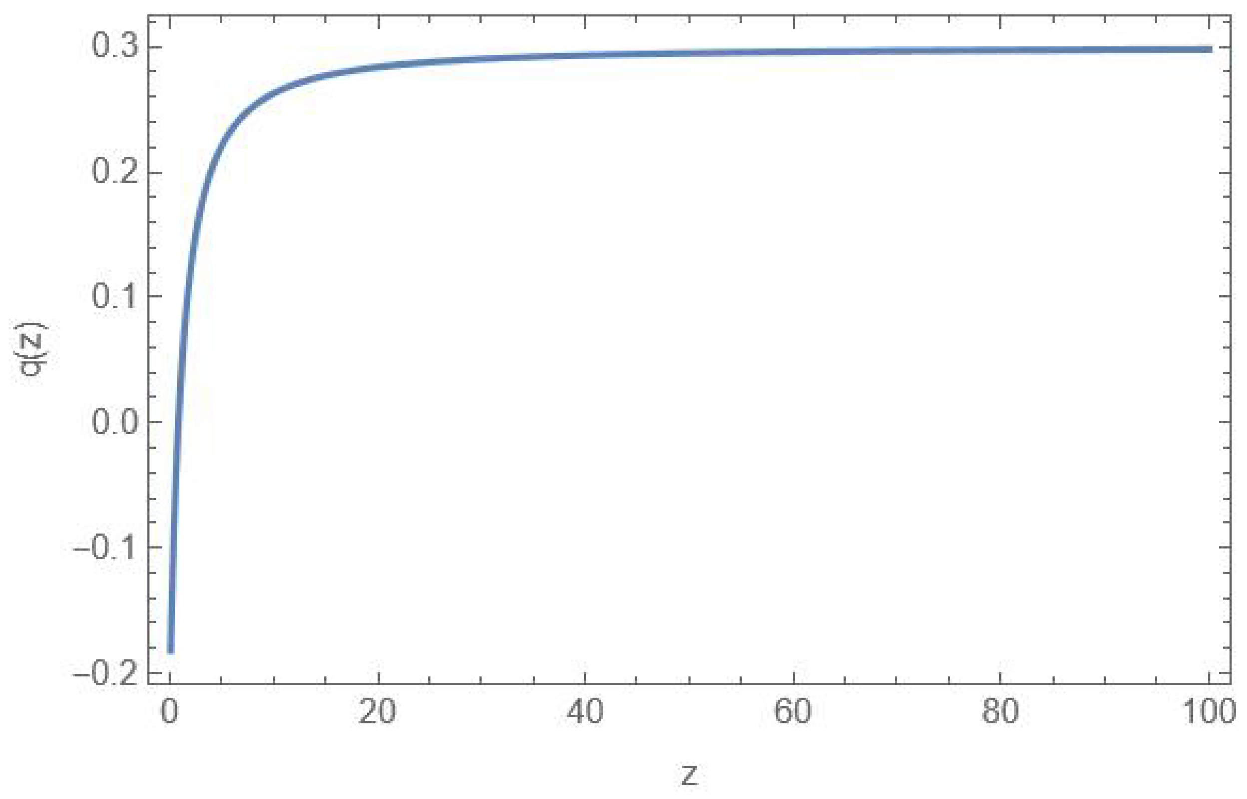
From Figure 1, the plot of the deceleration parameter $q\left(z\right)$ shows that the universe is currently expanding at an accelerating rate, since $q\left(z\right)$ is negative at low redshift. As we move to higher redshift, $q\left(z\right)$ increases and crosses zero around $z\sim$ 0.5–0.7, indicating a transition from acceleration to deceleration. At earlier times, $q\left(z\right)$ becomes positive and approaches a nearly constant value around $0.3$, corresponding to a matter-dominated phase. The curve does not approach $q\approx 1$, suggesting that the radiation-dominated era is not explicitly captured. Overall, this behavior reflects a smooth transition from the present accelerated expansion to a decelerated phase in the past.

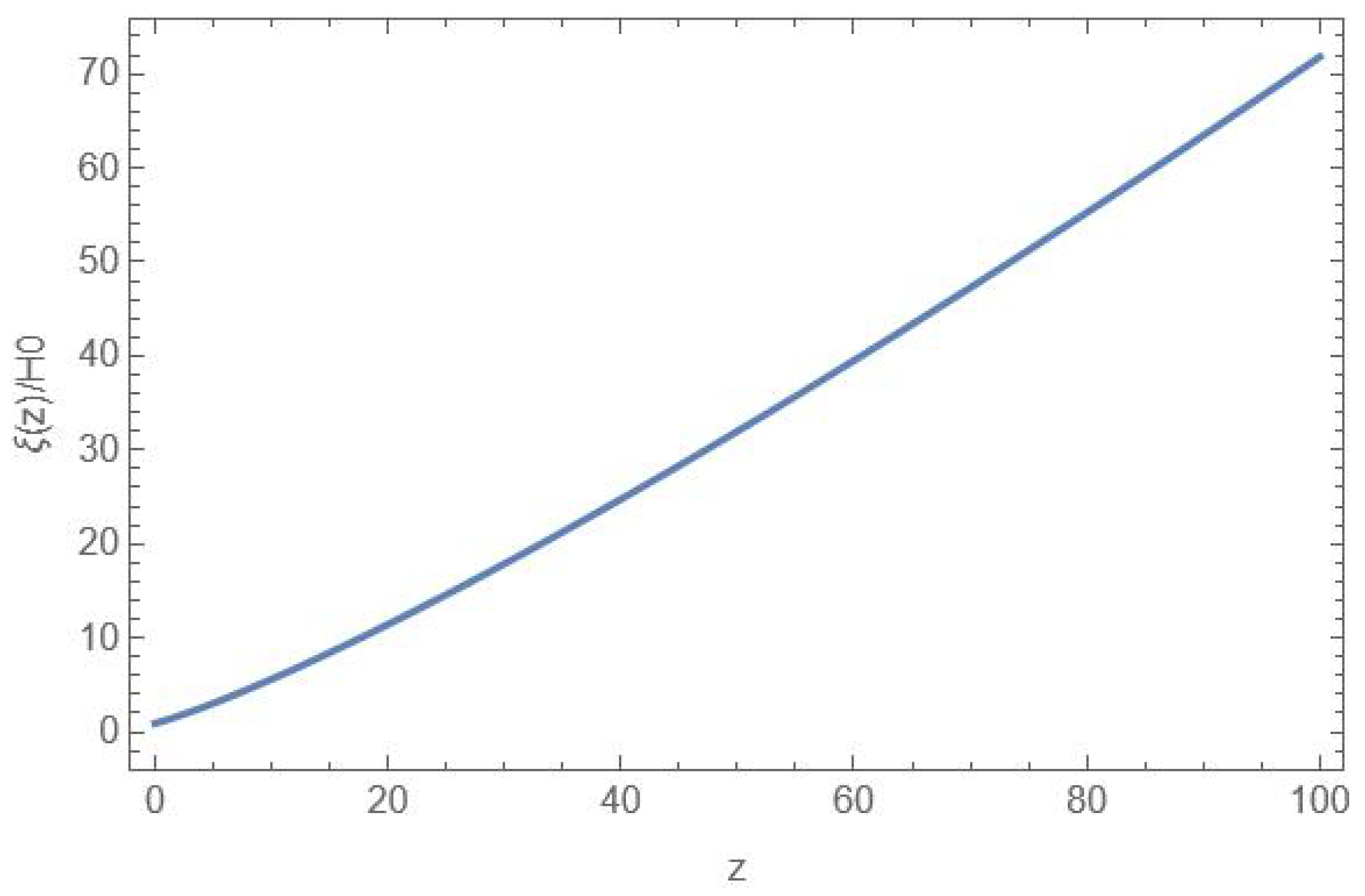
From Figure 2 it is clear that $\xi \ge 0$ over the full redshift range is constrained by observational data. Since entropy is proportional to $\xi H^2$, a positive $\xi$ ensures that the model is consistent with the thermodynamics. From the given parametrized form of $H\left(z\right)$, this validity tends to the constraints on $Y_2\le {\displaystyle \frac{3}{2}}$ and we impose $0\le Y_1\le 1$ to confirm the positivity of the Hubble parameter and $Y_1{Y}_2<1$ ensure about present-time acceleration. Furthermore, these conditions were incorporated as a prior in the analysis.

The above given observational

Table 1. Model constraints with statistical comparison table.

Data	Parameter	Best-Fit Value	${\mathit{\chi }}_{\mathbf{red}}^2$	AIC	BIC	$\mathsf{\Delta }$AIC	$\mathsf{\Delta }$BIC
H(z)	$H_0$	$64.471$	0.506	21.71	26.28	4.92	7.96
	$Y_1$	0.61
	$Y_2$	1.33
H(z) + DBAO	$H_0$	68.01	0.67	35.96	43.28	1.08	2.91
	$Y_1$	0.295
	$Y_2$	1.87
	$r_d$	146.72
H(z) + DBAO + PP	$H_0$	67.58	0.45	781.054	802.917	2.7	2.6
	$Y_1$	0.32
	$Y_2$	1.8309
	$r_d$	146.75

summarizes the best-fit values of the model parameters obtained from different combinations of observational datasets, namely the Hubble $H\left(z\right)$, DBAO, and Pantheon Plus datasets. The results show that the inclusion of additional datasets significantly improves the constraints on the model parameters and reduces the uncertainties associated with them.

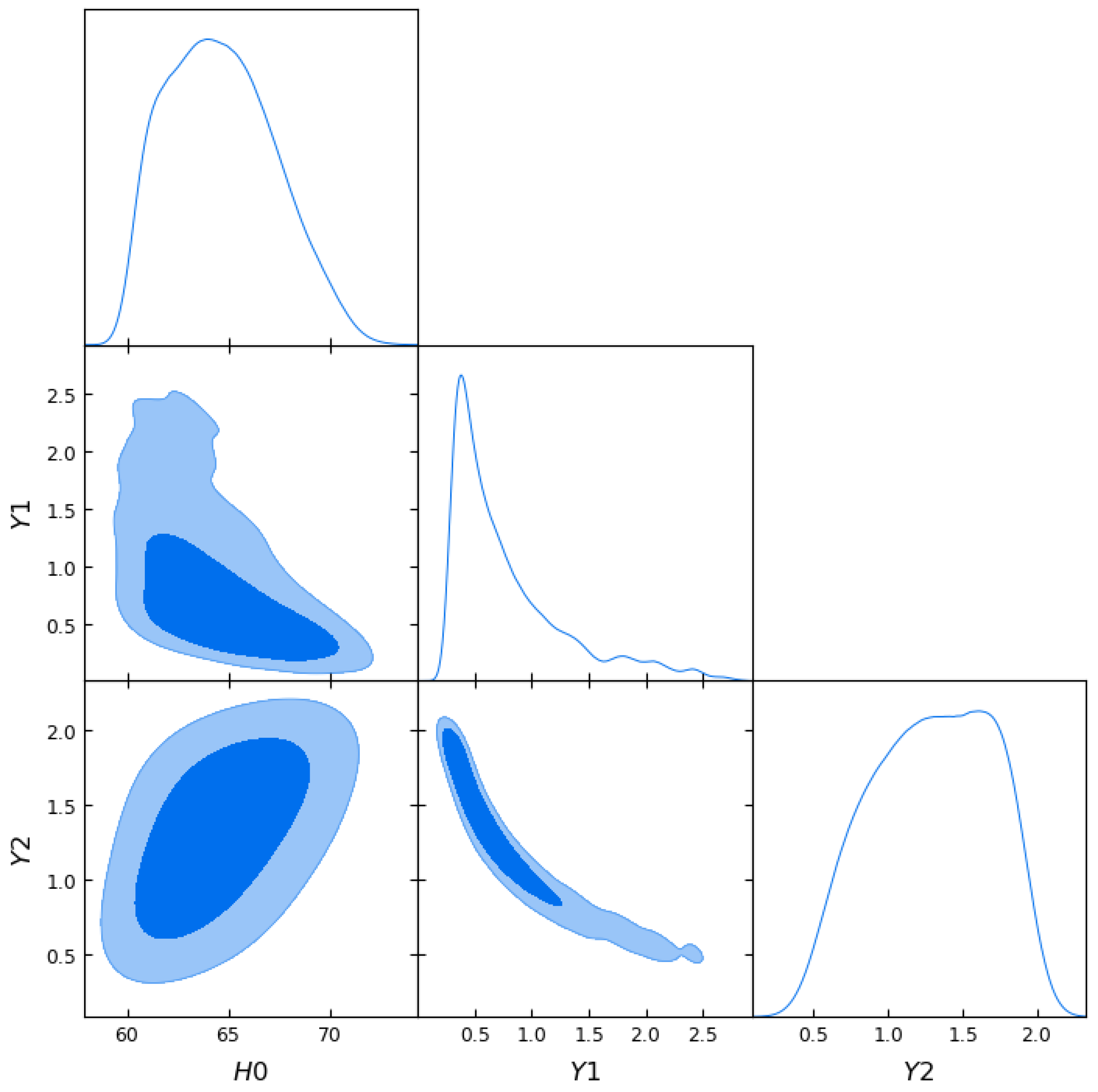
Using only the $H\left(z\right)$ dataset, corresponding to Figure 3, the model yields the best-fit values $H_0=64.47\mathrm{km}{\mathrm{s}}^{-1}{\mathrm{Mpc}}^{-1}$, $Y_1=0.61$, and $Y_2=1.33$. The reduced chi-square value ${\chi }_{\mathrm{red}}^2=0.506$ indicates that the model provides a good fit to the observational Hubble data. However, the comparatively larger values of $\mathsf{\Delta }$AIC and $\mathsf{\Delta }$BIC suggest that the statistical preference of the model is weaker when only the Hubble dataset is considered.

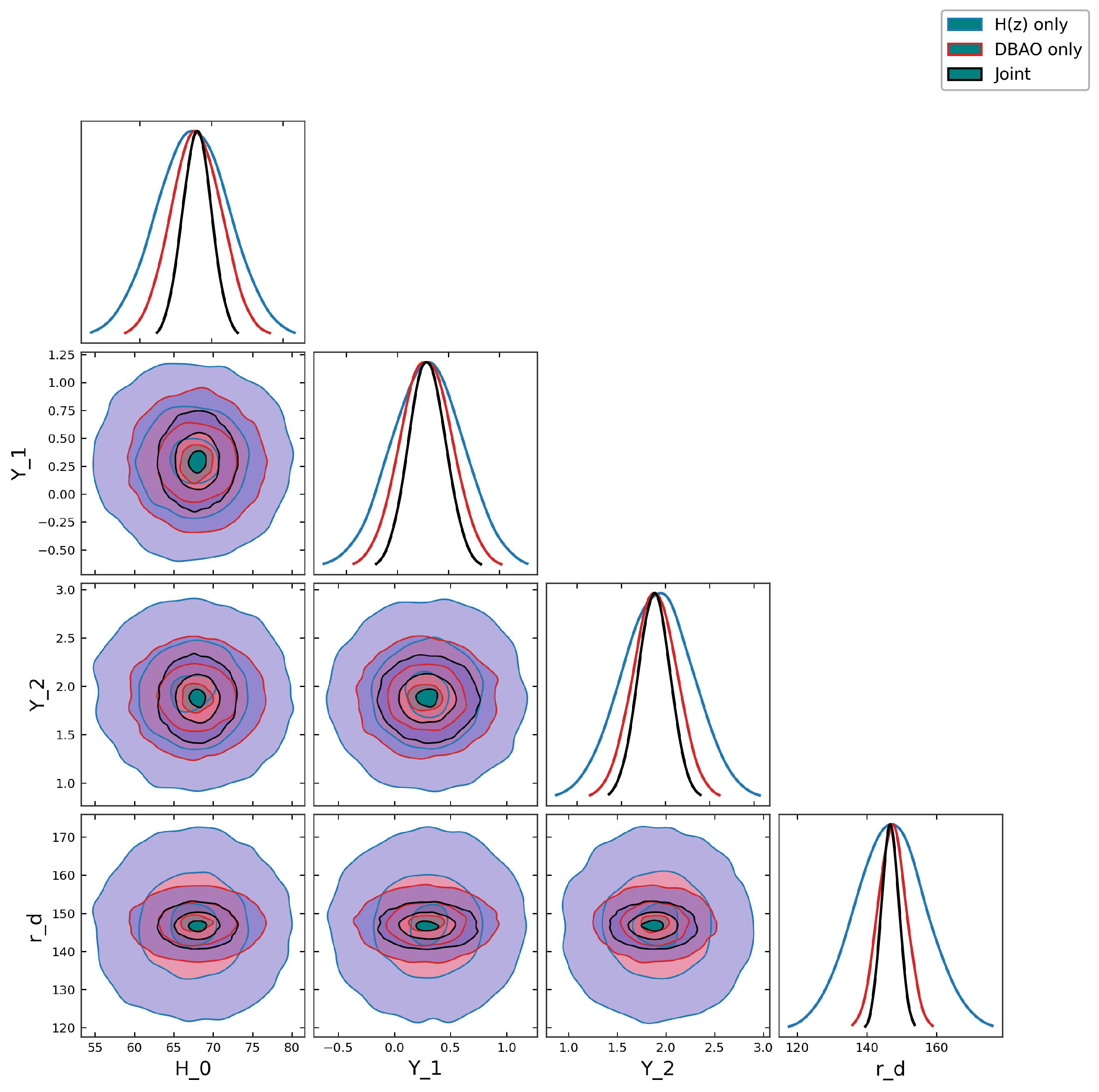
For the combined $H\left(z\right)+$ DBAO analysis shown in Figure 4, the parameter constraints become tighter, and the best-fit values shift to $H_0=68.01\mathrm{km}{\mathrm{s}}^{-1}{\mathrm{Mpc}}^{-1}$, $Y_1=0.295$, $Y_2=1.87$ and $r_d=146.75$ Mpc. The reduced chi-square value remains below unity, confirming the consistency of the model with the combined observational datasets. In addition, the smaller values of $\mathsf{\Delta }$AIC and $\mathsf{\Delta }$BIC indicate an improved statistical performance compared to the analysis using only $H\left(z\right)$ data.

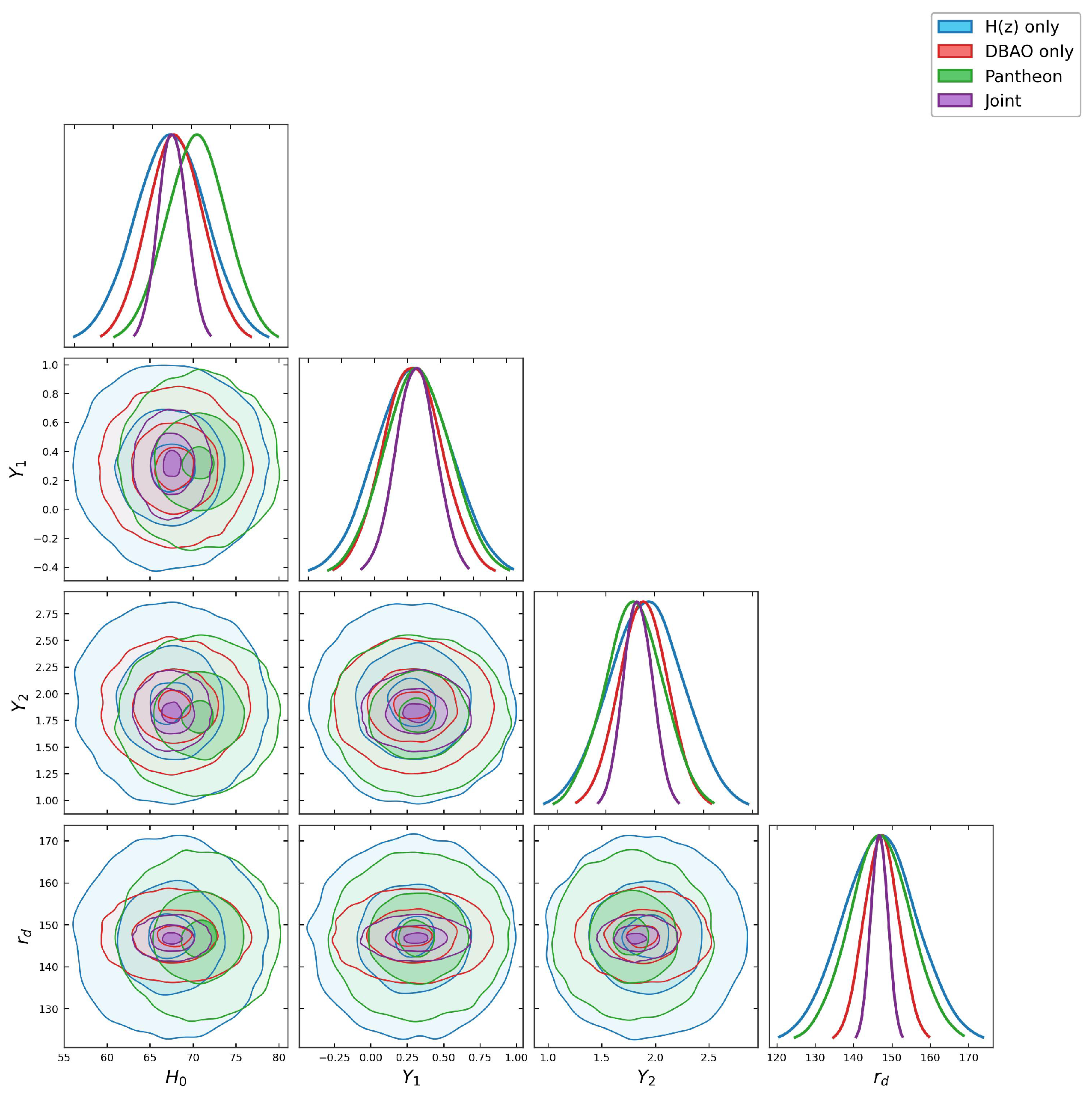
The joint analysis involving $H\left(z\right)$, DBAO, and Pantheon Plus datasets, illustrated in Figure 5, provides the strongest observational constraints on the model parameters. In this case, the best-fit values are obtained as $H_0=67.58\mathrm{km}{\mathrm{s}}^{-1}{\mathrm{Mpc}}^{-1}$, $Y_1=0.32$, $Y_2=1.8309$, and $r_d=146.75$ Mpc. The reduced chi-square value ${\chi }_{\mathrm{red}}^2=0.45$ demonstrates an excellent agreement between the theoretical model and the observational data. Furthermore, the relatively small values of $\mathsf{\Delta }$AIC and $\mathsf{\Delta }$BIC suggest that the model remains observationally viable and statistically competitive when all datasets are considered together.

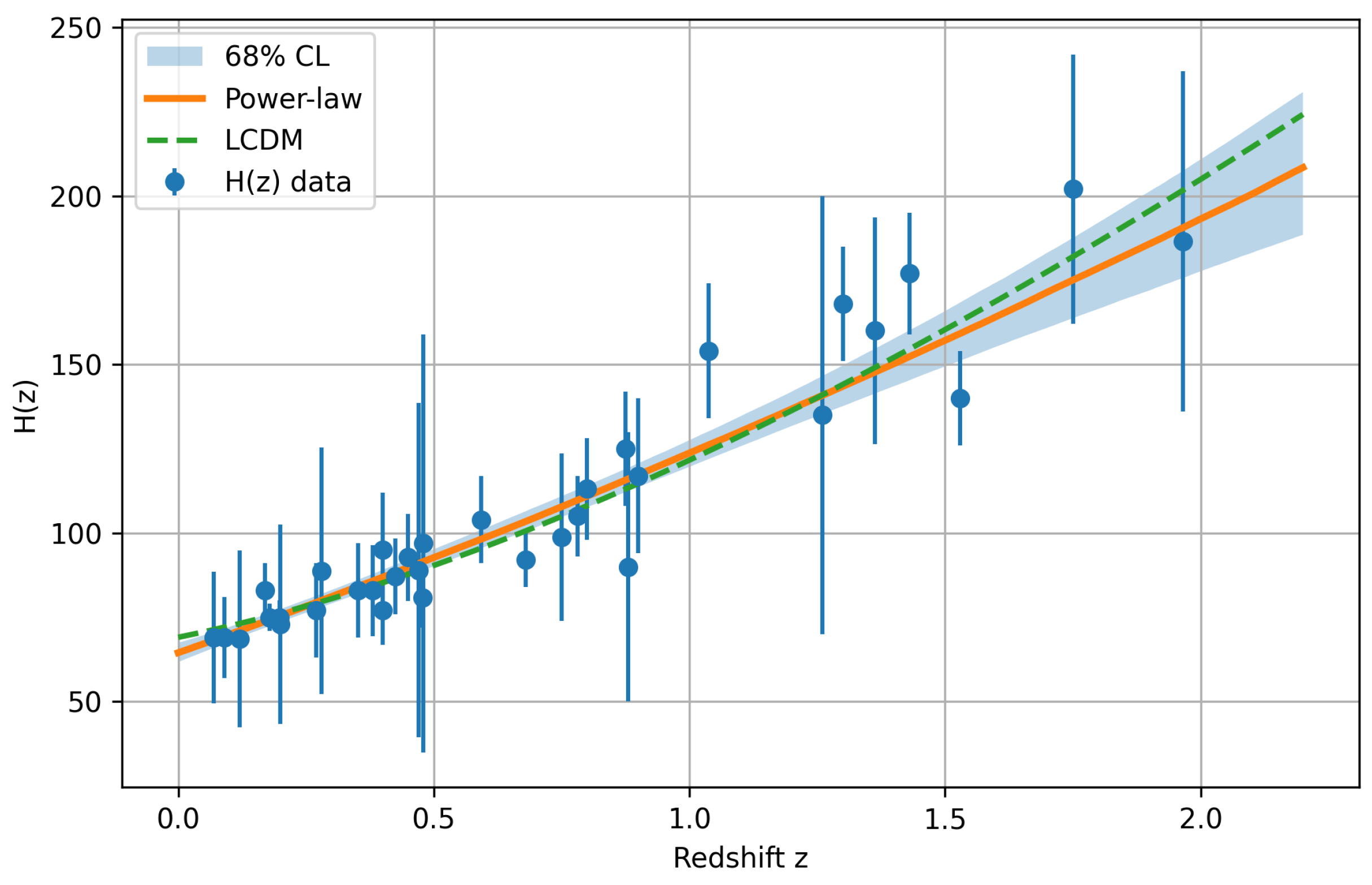
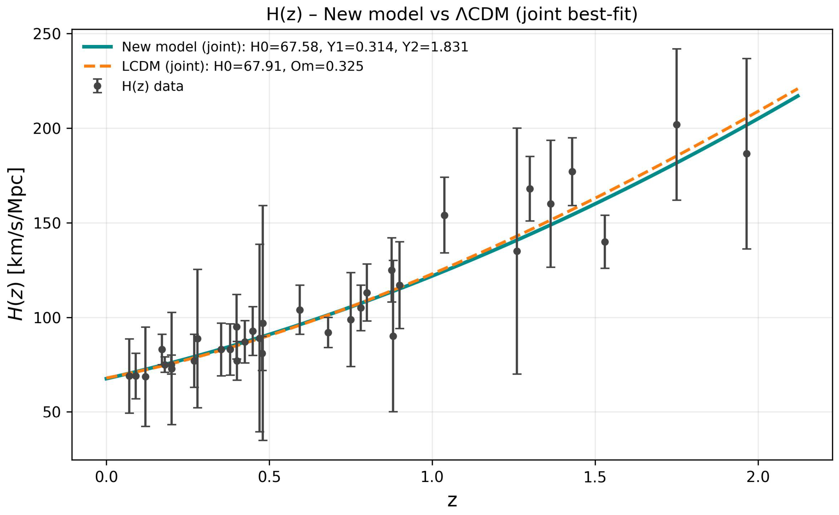
Figure 6 shows the evolution of $H\left(z\right)$ using only the Hubble dataset, where the model provides a reasonable fit but with relatively larger uncertainties. In contrast, Figure 7, based on the joint dataset, exhibits significantly tighter constraints and a more precise reconstruction of the expansion history. At low redshift, both the proposed model and $\mathsf{\Lambda }$CDM follow nearly identical trends, indicating similar expansion behavior, while at higher redshift, small deviations appear but remain within observational uncertainties [79,80].

The $\mathsf{\Lambda }$CDM model is consistent with both background expansion and structure formation, as it correctly describes the growth of density perturbations that lead to the observed large-scale distribution of galaxies and clusters. It is tightly constrained by the CMB anisotropy spectrum, where the acoustic peak structure determines key cosmological parameters, including ${\mathrm{\Omega }}_m$ and the baryon content. The value ${\mathrm{\Omega }}_m\approx 0.3$ is robustly supported through combined analyses of CMB, BAO, and large-scale structure observations, ensuring consistency across multiple independent probes. This agreement indicates that the model is consistent with the observed Hubble data within the statistical limits of the measurements. The close alignment between theory and observation supports the reliability of the underlying cosmological assumptions and shows that the parametrization effectively captures the dynamical behavior governing the expansion of the universe.

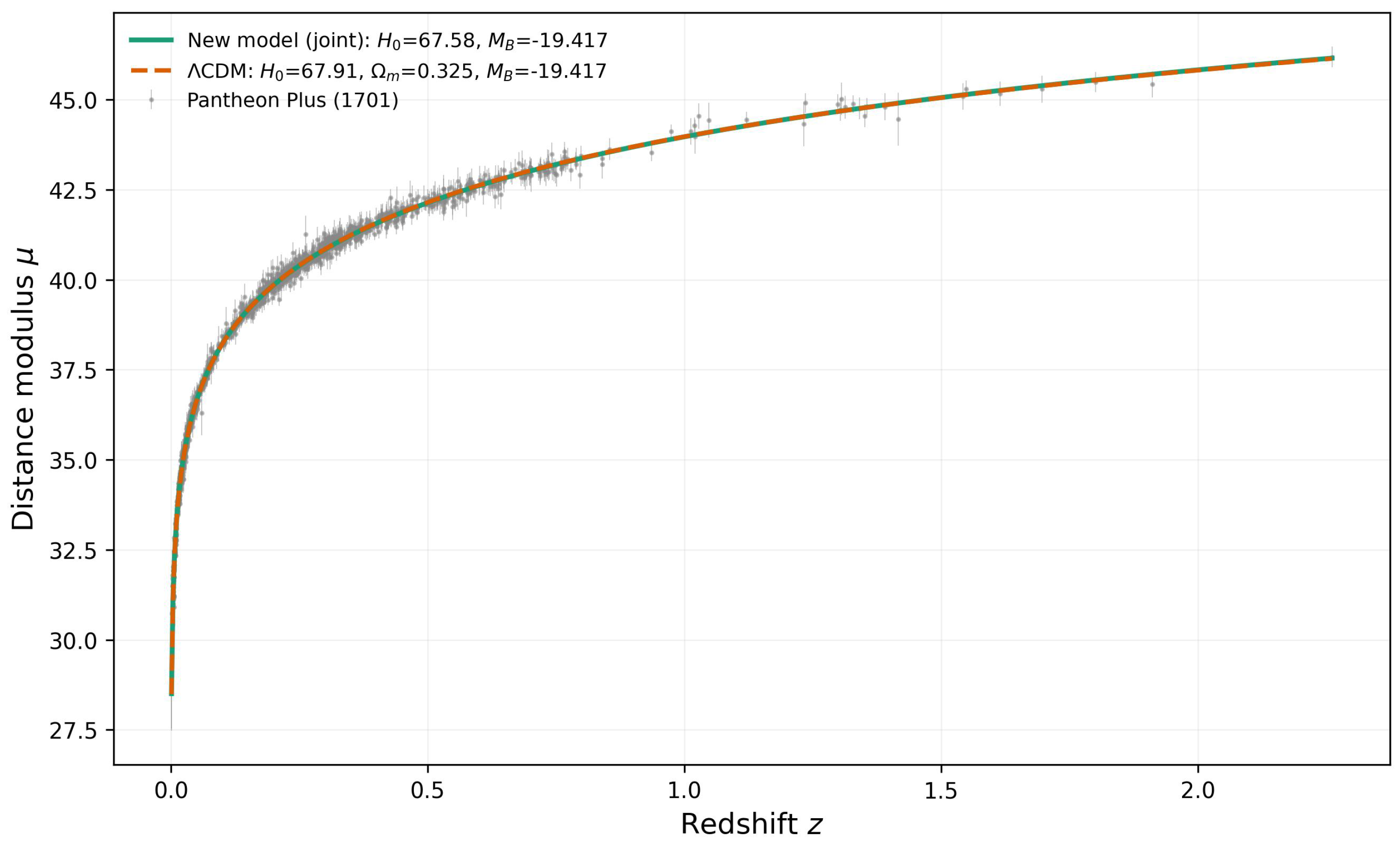
In Figure 8, the best-fit curve for the Pantheon Plus dataset at $H_0=67.59\mathrm{km}{\mathrm{s}}^{-1}{\mathrm{Mpc}}^{-1}$, illustrated by the teal solid curve, expresses the optimized luminosity–distance relation that most accurately reproduces the observed Type Ia supernova magnitudes. In contrast, the dashed violet curve corresponds to the prediction from the standard $\mathsf{\Lambda }CDM$ cosmological model. A comparison between the two reveals that both curves follow the Pantheon Plus observations closely over the full redshift range, with only minor deviations within statistical uncertainties. This high degree of overlap indicates that the best-fit parametrization captures the expansion history with effectiveness comparable to $\mathsf{\Lambda }CDM$, thereby providing a robust and consistent description of the underlying cosmological dynamics.

5. Conclusions

In this work, we conducted an extensive MCMC analysis to restrain an inhomogeneous equation of state for a viscous cosmic fluid. Using three dataset H(z) data, DESI BAO measurements and the Pantheon Plus sample, we were able to tightly constrain the model parameters and evaluate the consistency of the viscous fluid framework with current cosmological observations.

Bayesian inference and MCMC sampling together form a rigorous and highly effective statistical framework for cosmological parameter estimation. Through the careful construction of likelihoods, selection of priors, execution of MCMCs, and implementation of convergence diagnostics, we obtain robust observational constraints $H_0\in (64,70)\mathrm{km}{\mathrm{s}}^{-1}{\mathrm{Mpc}}^{-1}$ and $r_d=146\pm 0.75$ Mpc, with the value of constant $Y_1$ as well as $Y_2$. Those values shown in the observation table demonstrate that the viscous inhomogeneous model exhibits compatibility with the behavior of late-time cosmological expansion. The observational constraints best fit the value as $Y_1<1$ and $Y_2\le 2$. At high redshift, as $z\to \infty$, the deceleration parameter q tends to $Y_2-1$, which is only dependent on the fitted value of $Y_2$. For the best-fit parameter, the model exhibits effective matter-like behavior over intermediate redshift values, while at very high redshift it approaches a fixed limit due to its single power-law form and does not simultaneously reproduce both matter- and radiation-dominated epochs. The thermodynamic consistency of the model, by verifying that the bulk viscosity coefficient $\xi \left(z\right)$ remains non-negative over the entire redshift range constrained by the observational data, ensures positive entropy production which ensures the accelerated expansion of the universe thermodynamically.

To further test the viability of the proposed viscous inhomogeneous model, we plan to extend this analysis by incorporating additional observational datasets, including redshift space distortion (RSD) measurements, and the Union3 supernova compilation. We further aim to explore the perturbative regime of the proposed model to investigate the growth of large-scale structures using RSD data. Additionally, we will examine the implications of the viscous inhomogeneous model for current cosmological tensions, such as the $H_0$ and $S_8$ discrepancies, by incorporating Cosmic Microwave Background (CMB) observations. These aspects will be addressed in future work.

References

1. Nojiri, S.; Odintsov, S.D. Unified cosmic history in modified gravity: From F(R) theory to Lorentz non-invariant models. Phys. Rep. 2011, 505, 59–144. [Google Scholar] [CrossRef]
2. Meng, X.H.; Wang, P. Modified Friedmann equations in R−1-modified gravity. Class. Quantum Gravity 2003, 20, 4949. [Google Scholar] [CrossRef]
3. Meng, X.H.; Wang, P. Cosmological evolution in 1/R-gravity theory. Class. Quantum Gravity 2004, 21, 951. [Google Scholar] [CrossRef]
4. Meng, X.H.; Wang, P. R2 corrections to the cosmological dynamics of inflation in the Palatini formulation. Class. Quantum Gravity 2004, 21, 2029. [Google Scholar] [CrossRef]
5. Meng, X.H.; Wang, P. Gravitational potential in the Palatini formulation of modified gravity. Gen. Relativ. Gravit. 2004, 36, 1947–1954. [Google Scholar] [CrossRef]
6. Meng, X.H.; Hu, M.G.; Ren, J. Cosmology with extended Chaplygin gas and ω = −1 crossing. arXiv 2005, arXiv:astro-ph/0510357. [Google Scholar] [CrossRef]
7. Flanagan, E.E. Higher-order gravity theories and scalar–tensor theories. Class. Quantum Gravity 2003, 21, 417. [Google Scholar] [CrossRef]
8. Nojiri, S.; Odintsov, S.D. Where new gravitational physics comes from: M-theory? Phys. Lett. B 2003, 576, 5–11. [Google Scholar] [CrossRef]
9. Nojiri, S.; Odintsov, S.D. Modified gravity with negative and positive powers of curvature. Phys. Rev. D 2003, 68, 123512. [Google Scholar] [CrossRef]
10. Nojiri, S.I.; Odintsov, S.D. Quantum de Sitter cosmology and phantom matter. Phys. Lett. B 2003, 562, 147–152. [Google Scholar] [CrossRef]
11. Weinberg, S. Entropy generation and the survival of protogalaxies. Astrophys. J. 1971, 168, 175. [Google Scholar] [CrossRef]
12. Padmanabhan, T.; Chitre, S.M. Viscous universes. Phys. Lett. A 1987, 120, 433–436. [Google Scholar] [CrossRef]
13. Grøn, Ø. Viscous inflationary universe models. Astrophys. Space Sci. 1990, 173, 191–225. [Google Scholar] [CrossRef]
14. Brevik, I.; Hallanger, A. Randall—Sundrum model with bulk viscosity. Phys. Rev. D 2004, 69, 24009. [Google Scholar] [CrossRef]
15. Cataldo, M.; Cruz, N.; Lepe, S. Viscous dark energy and phantom evolution. Phys. Lett. B 2005, 619, 5–10. [Google Scholar] [CrossRef]
16. Brevik, I.; Heen, L.T. Remarks on the viscosity concept in the early universe. Astrophys. Space Sci. 1994, 219, 99–115. [Google Scholar] [CrossRef][Green Version]
17. Nojiri, S.I.; Odintsov, S.D. Inhomogeneous equation of state of the universe: Phantom era, future singularity, and crossing the phantom barrier. Phys. Rev. D 2005, 72, 23003. [Google Scholar] [CrossRef]
18. Nojiri, S.I.; Odintsov, S.D.; Tsujikawa, S. Properties of singularities in the (phantom) dark energy universe. Phys. Rev. D 2005, 71, 63004. [Google Scholar] [CrossRef]
19. Capozziello, S.; Cardone, V.F.; Elizalde, E.; Nojiri, S.I.; Odintsov, S.D. Observational constraints on dark energy with generalized equations of state. Phys. Rev. D 2006, 73, 43512. [Google Scholar] [CrossRef]
20. Brevik, I.; Gorbunova, O.; Shaido, Y.A. Viscous FRW cosmology in modified gravity. Int. J. Mod. Phys. D 2005, 14, 1899–1906. [Google Scholar] [CrossRef]
21. Brevik, I.; Gorbunova, O. Dark energy and viscous cosmology. Gen. Relativ. Gravit. 2005, 37, 2039–2045. [Google Scholar] [CrossRef]
22. Brevik, I.; Børven, J.M.; Ng, S. Viscous brane cosmology with a brane-bulk energy interchange term. Gen. Relativ. Gravit. 2006, 38, 907–915. [Google Scholar] [CrossRef]
23. Li, B.; Barrow, J.D. Does bulk viscosity create a viable unified dark matter model? Phys. Rev. D 2009, 79, 103521. [Google Scholar] [CrossRef]
24. Feng, C.J.; Li, X.Z. Viscous Ricci dark energy. Phys. Lett. B 2009, 680, 355–358. [Google Scholar] [CrossRef]
25. Babichev, E.; Dokuchaev, V.; Eroshenko, Y. Dark energy cosmology with generalized linear equation of state. Class. Quantum Gravity 2004, 22, 143. [Google Scholar] [CrossRef]
26. Jaffe, T.R.; Banday, A.J.; Eriksen, H.K.; Górski, K.M.; Hansen, F.K. Evidence of vorticity and shear at large angular scales in the WMAP data: A violation of cosmological isotropy? Astrophys. J. 2005, 629, L1. [Google Scholar] [CrossRef]
27. Zimdahl, W. Bulk viscous cosmology. Phys. Rev. D 1996, 53, 5483. [Google Scholar] [CrossRef]
28. Coley, A.A.; Van den Hoogen, R.J.; Maartens, R. Qualitative viscous cosmology. Phys. Rev. D 1996, 54, 1393. [Google Scholar] [CrossRef]
29. Chimento, L.P.; Jakubi, A.S.; Méndez, V.; Maartens, R. Cosmological solutions with nonlinear bulk viscosity. Class. Quantum Gravity 1997, 14, 3363. [Google Scholar] [CrossRef]
30. Brevik, I.; Grøn, Ø.; de Haro, J.; Odintsov, S.D.; Saridakis, E.N. Viscous cosmology for early- and late-time universe. Int. J. Mod. Phys. D 2017, 26, 1730024. [Google Scholar] [CrossRef]
31. Dou, X.; Meng, X.H. Bulk viscous cosmology: Unified dark matter. Adv. Astron. 2011, 2011, 829340. [Google Scholar] [CrossRef]
32. Normann, B.D.; Brevik, I. Characteristic properties of two different viscous cosmology models for the future universe. Mod. Phys. Lett. A 2017, 32, 1750026. [Google Scholar] [CrossRef]
33. Quercellini, C.; Bruni, M.; Balbi, A. Affine equation of state from quintessence and k-essence fields. Class. Quantum Gravity 2007, 24, 5413. [Google Scholar] [CrossRef]
34. Pietrobon, D.; Balbi, A.; Bruni, M.; Quercellini, C. Affine parametrization of the dark sector: Constraints from WMAP5 and SDSS. Phys. Rev. D 2008, 78, 83510. [Google Scholar] [CrossRef]
35. Arbey, A. Is it possible to consider dark energy and dark matter as a unique dark fluid? arXiv 2005, arXiv:astro-ph/0506732. [Google Scholar] [CrossRef]
36. Barrow, J.D. Graduated inflationary universes. Phys. Lett. B 1990, 235, 40–43. [Google Scholar] [CrossRef]
37. Bento, M.C.; Bertolami, O.; Sen, A.A. Generalized Chaplygin gas and dark-energy-matter unification. Phys. Rev. D 2002, 66, 43507. [Google Scholar] [CrossRef]
38. Zhu, Z.H. Generalized Chaplygin gas constraints. Astron. Astrophys. 2004, 423, 421–426. [Google Scholar] [CrossRef]
39. Amendola, L.; Finelli, F.; Burigana, C.; Carturan, D. WMAP and the generalized Chaplygin gas. J. Cosmol. Astropart. Phys. 2003, 2003, 5. [Google Scholar] [CrossRef]
40. Capozziello, S.; Nojiri, S.; Odintsov, S.D. Unified phantom cosmology: Inflation, dark energy and dark matter. Phys. Lett. B 2006, 632, 597–604. [Google Scholar] [CrossRef]
41. Brevik, I. Crossing of the ω = −1 barrier in viscous modified gravity. Int. J. Mod. Phys. D 2006, 15, 767–775. [Google Scholar] [CrossRef]
42. Nojiri, S.; Odintsov, S.D. Unifying phantom inflation with late-time acceleration. Gen. Relativ. Gravit. 2006, 38, 1285–1304. [Google Scholar] [CrossRef]
43. Thakran, B.; Dhankar, P.K.; Raut, S.; Ray, S.; Maurya, S.K.; Sanyal, A. Cosmological constraints on interacting holographic dark energy and extended Chaplygin gas in using MCMC analysis. Int. J. Geom. Methods Mod. Phys. 2025, 23, 2550254. [Google Scholar] [CrossRef]
44. Shukla, B.K.; Beesham, A.; Sofuoğlu, D.; Mishra, P.; Dubey, R.K. Cosmological model with parametrized Hubble parameter in f(R,T) gravity. Int. J. Mod. Phys. A 2025, 40, 2550048. [Google Scholar] [CrossRef]
45. Shukla, B.K.; Tiwari, R.K.; Sofuoğlu, D. Observational constraints in f(R,G) gravity. Int. J. Geom. Methods Mod. Phys. 2023, 20, 2350210. [Google Scholar] [CrossRef]
46. Bhardwaj, V.K.; Yadav, A.K.; Gupta, L.K.; Prasad, R.; Srivastava, S.K. Constraining scalar field cosmological model in Lyra geometry. Int. J. Geom. Methods Mod. Phys. 2025, 22, 2450283. [Google Scholar] [CrossRef]
47. Bhardwaj, V.K.; Yadav, A.K. Scalar field cosmology in anisotropic universe. Int. J. Geom. Methods Mod. Phys. 2024, 21, 2450144. [Google Scholar] [CrossRef]
48. Singh, G.P.; Garg, R.; Singh, A. Generalized ΛCDM model with viscous effects. Int. J. Geom. Methods Mod. Phys. 2025, 22, 2550111. [Google Scholar] [CrossRef]
49. Mazumdar, R.; Gohain, M.M.; Bhuyan, K. Cosmological bounce with bulk viscosity. Int. J. Geom. Methods Mod. Phys. 2025, 22, 2450292. [Google Scholar] [CrossRef]
50. Melia, F. Physical basis for the symmetries in the FRW metric. Front. Phys. 2016, 11, 119801. [Google Scholar] [CrossRef]
51. Khadekar, G.S.; Raut, D.; Miskin, V.G. FRW viscous cosmology with inhomogeneous equation of state. Mod. Phys. Lett. A 2015, 30, 1550144. [Google Scholar] [CrossRef]
52. Meng, X.H.; Ma, Z.Y. Rip/singularity free cosmology models with bulk viscosity. Eur. Phys. J. C 2012, 72, 2053. [Google Scholar] [CrossRef]
53. Khadekar, G.S.; Raut, D. FRW viscous fluid cosmology with time-dependent equation of state. Int. J. Geom. Methods Mod. Phys. 2018, 15, 1830001. [Google Scholar] [CrossRef]
54. Dhankar, P.K.; Sanyal, A.; Munyeshyaka, A.; Ray, S.; Pourhassan, B. Observational analysis of bulk viscous modified Chaplygin gas. arXiv 2025, arXiv:2504.18612. [Google Scholar] [CrossRef]
55. Tomasetti, E.; Moresco, M.; Borghi, N.; Jiao, K.; Cimatti, A.; Pozzetti, L.; Carnall, A.; McLure, R.; Pentericci, L. A new measurement of the expansion history of the Universe at z = 1.26 with cosmic chronometers in VANDELS. Astron. Astrophys. 2023, 679, A96. [Google Scholar] [CrossRef]
56. Jiao, K.; Borghi, N.; Moresco, M.; Zhang, T.J. New observational H (z) data from full-spectrum fitting of cosmic chronometers in the LEGA-C survey. Astrophys. J. Suppl. Ser. 2023, 265, 48. [Google Scholar] [CrossRef]
57. Borghi, N.; Moresco, M.; Cimatti, A. Toward a better understanding of cosmic chronometers: A new measurement of H(z) at z 0.7. Astrophys. J. Lett. 2022, 928, L4. [Google Scholar] [CrossRef]
58. Pantheon + SH0ES Collaboration. Pantheon + SH0ES Data Release. 2022. Available online: https://github.com/PantheonPlusSH0ES/DataRelease (accessed on 12 May 2026).
59. Patel, R.; Dhankar, P.K.; Islam, S.; Aamir, M. Data analysis in (2+1)-D Λ(z) gravity with BAO, Pantheon and Hubble dataset using MCMC method. Indian J. Phys. 2026, 1–11. [Google Scholar] [CrossRef]
60. Speagle, J.S. A conceptual introduction to Markov Chain Monte Carlo methods. arXiv 2019, arXiv:1909.12313. [Google Scholar] [CrossRef]
61. Trotta, R. Bayes in the sky: Bayesian inference in cosmology. Contemp. Phys. 2008, 49, 71–104. [Google Scholar] [CrossRef]
62. Noh, Y.; Choi, K.K.; Lee, I. Comparison of MCMC-based Bayesian methods. Struct. Multidiscip. Optim. 2010, 42, 823–833. [Google Scholar] [CrossRef]
63. Lougheed, B.C.; Obrochta, S.P. MatCal: Bayesian 14C age calibration. J. Open Res. Softw. 2016, 4, e42. [Google Scholar] [CrossRef]
64. Bernardo, J.M. Bayesian statistics. In International Encyclopedia of Statistical Science; Springer: Berlin/Heidelberg, Germany, 2011; pp. 107–133. [Google Scholar]
65. Akaike, H. A new look at the statistical model identification. IEEE Trans. Autom. Control 2003, 19, 716–723. [Google Scholar] [CrossRef]
66. Schwarz, G. Estimating the dimension of a model. Ann. Stat. 1978, 6, 461–464. [Google Scholar] [CrossRef]
67. Mandal, S.; Pradhan, S.; Sahoo, P.K.; Harko, T. Cosmological constraints on power-law f(Q) gravity. Eur. Phys. J. C 2023, 83, 1141. [Google Scholar] [CrossRef]
68. Li, Z.; Zhang, B.; Liang, N. Testing dark energy models with gamma-ray bursts calibrated from the observational H(z) data through a Gaussian process. Mon. Not. R. Astron. Soc. 2023, 521, 4406–4413. [Google Scholar] [CrossRef]
69. Dhankar, P.K.; Sanyal, A.; Islam, S.; Rahaman, F.; Pourhassan, B. Testing the generalized second law in (2+1)-D cosmology. arXiv 2025, arXiv:2508.13227. [Google Scholar] [CrossRef]
70. Koussour, M.; Myrzakulov, N.; Ali, M.K.M. Exploring universe acceleration via observational constraints. J. High Energy Astrophys. 2024, 42, 96–103. [Google Scholar] [CrossRef]
71. Adame, A.G.; Aguilar, J.; Ahlen, S.; Alam, S.; Alexander, D.M.; Alvarez, M.; Alves, O.; Anand, A.; Andrade, U.; Armengaud, E. DESI 2024 II: Sample definitions, characteristics, and two-point clustering statistics. J. Cosmol. Astropart. Phys. 2025, 7, 17. [Google Scholar] [CrossRef]
72. Zhou, R. Target selection and validation of DESI luminous red galaxies. Astron. J. 2023, 165, 58. [Google Scholar] [CrossRef]
73. Adame, A.G. DESI 2024 III: Baryon acoustic oscillations from galaxies and quasars. J. Cosmol. Astropart. Phys. 2025, 4, 12. [Google Scholar] [CrossRef]
74. Raichoor, A. Target selection and validation of DESI emission line galaxies. Astron. J. 2023, 165, 126. [Google Scholar] [CrossRef]
75. Chaussidon, E. Target selection and validation of DESI quasars. Astrophys. J. 2023, 944, 107. [Google Scholar] [CrossRef]
76. Adame, A.G. DESI 2024 IV: Baryon acoustic oscillations from the Lyman-alpha forest. J. Cosmol. Astropart. Phys. 2025, 1, 124. [Google Scholar] [CrossRef]
77. Bouali, A. Data analysis of three-parameter models of the deceleration parameter in FLRW universe. Eur. Phys. J. Plus 2023, 138, 844. [Google Scholar] [CrossRef]
78. Conley, A.; Guy, J.; Sullivan, M.; Regnault, N.; Astier, P.; Balland, C.; Basa, S.; Carlberg, R.G.; Fouchez, D.; Hardin, D. Supernova Constraints and Systematic Uncertainties from the First 3 Years of the Supernova Legacy Survey. Astrophys. J. Suppl. 2011, 192, 1. [Google Scholar] [CrossRef]
79. Sahni, V.; Starobinsky, A. Reconstructing Dark Energy. Int. J. Mod. Phys. D 2006, 15, 2105–2132. [Google Scholar] [CrossRef]
80. Basilakos, S.; Plionis, M.; Solà, J. Hubble expansion and structure formation in time varying vacuum models. Phys. Rev. D 2009, 80, 83511. [Google Scholar] [CrossRef]
Figure 1. 2D variation of the deceleration parameter q ( z ) versus z. The diagram depicts the evolution of the deceleration parameter q ( z ) over the range 0 z 100 for Y 1 = 0.7 and Y 2 = 1.3 . The behavior reveals important features of the cosmic expansion history.
Mathematics 14 01888 g001
Figure 2. Viscosity coefficient as a function of redshift parameter. The variation is shown for constant values ξ 0 = 0.5 , ξ 1 = 0.3 , ξ 2 = 0.1 , Y 1 = 0.7 , and Y 2 = 1.2 .
Mathematics 14 01888 g002
Figure 3. Corner plots for the Hubble dataset are obtained using Equation (31) for the viscous fluid model. The contours represent the constraints on model parameters and their mutual correlations, demonstrating the model’s consistency with observational expansion data.
Mathematics 14 01888 g003
Figure 4. Joint corner plots for the H ( z ) and DESI BAO datasets obtained using Equation (31) for the viscous fluid model. The contours show the combined constraints on model parameters and their correlations, demonstrating consistency with both expansion and clustering observations.
Mathematics 14 01888 g004
Figure 5. Joint triangle plots for the Hubble, DESI BAO, and Pantheon Plus datasets using Equation (31) for the viscous fluid model. The combined analysis helps in better constraining the model parameters and understanding their correlations.
Mathematics 14 01888 g005
Figure 6. Error plot for the Hubble dataset with the Λ CDM model. The plot shows the difference between observational data and model predictions.
Mathematics 14 01888 g006
Figure 7. Joint best-fit curve for the Hubble, DESI BAO, and Pantheon Plus datasets using Equation (31) for the viscous fluid model, compared with the Λ CDM model. The plot shows how both models fit the combined observational data.
Mathematics 14 01888 g007
Figure 8. Best-fit curve of the distance modulus μ ( z ) compared with the Λ CDM prediction for the given viscous model defined in Equation (31), along with the observational data.
Mathematics 14 01888 g008