Sequential Estimation for Monitoring One-Shot Device Stockpiles

Abstract

One-shot devices yield binary current-status observations because each unit can be tested only once. In stockpile settings, where testing is destructive and failures are rare, fixed-sample plans may consume more units than necessary. This paper proposes a sequential estimation procedure for monitoring one-shot device stockpiles at a fixed inspection time. The method is formulated in terms the inspection-time failure probability and its reciprocal, and is therefore applicable to general one-parameter lifetime models. A squared-error-plus-sampling-cost risk function is used to derive a stopping rule that adaptively determines the required number of observed failures. We establish first-order efficiency relative to an optimal fixed-sample benchmark and illustrate the framework through a stockpile case study motivated by stored N95 respirators. The proposed procedure provides a practical and theoretically justified tool for stockpile monitoring when destructive testing is costly and unnecessary sampling should be minimized.

1. Introduction

Research on survival analysis plays a central role in reliability analysis and life testing, where experiments are often expensive or time-consuming to conduct. To improve efficiency, sequential estimation of the exponential mean has been widely explored since the 1980s. Early work by Sen et al. [1] introduced time-sequential estimation incorporating both recruitment and monitoring costs. Stadje et al. [2] proposed a Bayesian sequential estimator, while Mukhopadhyay and co-authors developed a broad collection of sequential methodologies for comparing exponential means, constructing accelerated procedures, and studying bounded-risk estimation [3,4,5]. More recently, estimation of minimum-risk points under powered error loss has been studied in Mukhopadhyay and Khariton [6], and Mukhopadhyay and Li [7] extended purely sequential MRPE procedures to the estimation of survival probability.

In reliability applications, right-censoring naturally arises when items survive beyond the duration of the test, reducing testing cost; see Zhu et al. [8]. Sequential inference has also been examined for right-censored data. Gardiner and Susarla et al. [9] considered estimation of mean survival time under unspecified distributions, while Gardiner et al. [10] studied exponential mean estimation with random withdrawals. Aras et al. [11,12] further analyzed sequential properties under random censoring. Broader discussions of sequential analysis and MRPE appear in [13,14,15,16].

Despite this extensive literature, sequential estimation has received comparatively limited attention in reliability engineering. Some recent studies, such as Zhang et al. [17] on sequential degradation modeling and Houlding and Coolen [18] on sequential decision-making, address reliability problems but do not develop sequential parameter estimation methods tailored to reliability settings. This gap motivates the development of sequential procedures adapted to censoring structures commonly encountered in practice.

One-shot devices are systems that can function only once and are typically destroyed or rendered unusable after testing or activation. Examples include automotive pyrotechnic inflators, emergency medical auto-injectors, defibrillator shock cartridges, and aerospace ignition or separation actuators. In many reliability applications, such devices are tested destructively at a fixed inspection time, yielding only binary current-status data indicating whether failure has occurred by that time. A broad review of one-shot device data collection, modeling, and inference can be found in Balakrishnan, Ling, and So [19]. Because such devices cannot undergo repeated testing, manufacturers and regulatory agencies rely on statistically efficient inspection plans to ensure reliability at predetermined inspection times. The consequences of even rare failures can be severe. For instance, in 2021–2022, the U.S. Air Force temporarily grounded several aircraft fleets due to potential defects in ejection-seat components essential for aircrew survival [20].

Stockpile life assessment (SLA) concerns the reliability evaluation of systems that are stored for extended periods and are rarely used until activation. These systems are typically highly reliable and may undergo latent degradation during storage, with failure occurring only after degradation exceeds a critical threshold. Vander Wiel [21] proposed a random onset degradation model to describe this phenomenon, where degradation begins at an unknown time and leads to a sudden decline in system reliability. This framework aligns directly with the one-shot device setting considered in this paper, where each unit is tested only once at a specified inspection time. Consequently, SLA can be viewed as a direct application of the proposed sequential one-shot testing methodology.

Degradation-based reliability modeling plays a central role in SLA. In many applications, failure is defined through a threshold-crossing mechanism of an underlying degradation process. Si et al. [22] provide a comprehensive review of statistical degradation models for remaining useful life estimation, emphasizing stochastic process models and threshold-based failure definitions. The degradation model used in our numerical example, based on a gamma process with a failure threshold, is directly consistent with this framework and provides a realistic representation of aging mechanisms in stored systems.

Stockpile systems are often safety-critical and involve high-consequence applications such as missile components, defense systems, and personal protective equipment (PPE). These systems are typically one-shot in nature, meaning they are used only once and cannot be repeatedly tested. As noted in the reliability engineering literature of Elsayed [23] and stockpile studies by the National Research Council [24], failures in such systems can lead to severe consequences, including loss of life or mission failure. Recent work of Chen et al. [25] on storage reliability of missile systems further emphasizes the role of multi-component competitive failure mechanisms in modeling degradation and failure during long-term storage. Similarly, studies on stored PPE by Bergman et al. [26] and N95 respirators by Lin et al. [27] highlight the importance of assessing degradation over time to ensure safety in emergency use.

In this context, the proposed sequential testing framework provides a practical and efficient solution for SLA problems. By optimizing a risk function that balances estimation error and testing cost, the method reduces uncertainty in reliability assessment while limiting destructive testing. This is particularly important in stockpile settings where testing is destructive and resources are limited. The ability to obtain accurate reliability estimates with fewer tests enables safer utilization of stored one-shot systems and supports informed decision-making in high-stakes applications.

While sequential methodologies for exponential lifetimes are well developed, their use in one-shot device testing has received little attention. In this work, we extend the sequential estimation framework of Hu et al. [28] to the one-shot setting, where only current-status data are observed, and demonstrate that such procedures provide an efficient and principled approach to designing reliability experiments for single-use devices.

In this paper, we study one-shot devices inspected once at a fixed time $t_I$. Let T denote the lifetime of a device. The observable outcome is the current-status indicator

$$\delta =\mathbf{1}\{T\le t_I\},$$

so only whether failure has occurred by time $t_I$ is recorded. Accordingly, the failure probability at inspection is

$$p_f=\mathrm{Pr}(T\le t_I)=F(t_I\mid \theta ).$$

Following the sequential framework of Hu et al. [28], we repeatedly test devices at the same fixed inspection time $t_I$ and terminate the experiment once exactly r failures have been observed. In this setting, the total number of tested units N is random and follows a negative binomial distribution $N\sim \mathrm{NBin}(r,p_f)$. This sequential one-shot testing scheme naturally arises in reliability applications where testing each device is destructive and only a single inspection outcome can be recorded.

Our goal is to estimate reliability characteristics efficiently while consuming as few tested units as possible under a squared-error loss plus sampling cost. To this end, we develop a sequential estimation procedure adapted to the one-shot data structure, derive its large-sample properties, and investigate its practical performance through simulations.

Our main contributions are as follows. First, we adapt the sequential estimation framework of Hu et al. [28] to destructive one-shot device testing under binary current-status observations. Second, we establish first-order efficiency of the resulting stopping rule relative to the optimal fixed-sample benchmark. Third, we demonstrate through simulation that the proposed procedure attains near-optimal risk while reducing unnecessary testing. Finally, we illustrate how the sequential framework can be embedded in a stockpile–reliability assessment calibrated to published respirator degradation results.

The remainder of the paper is organized as follows. Section 2 presents the sequential estimation procedure for one-shot devices. Section 3 establishes its key asymptotic properties. Section 4 reports Monte Carlo results and an illustrative stockpile–reliability case study calibrated to published N95 respirator data. Lastly, we conclude with final remarks in Section 5.

2. Sequential Estimation Procedure

2.1. Observation Model and Likelihood

Under the one-shot testing framework described in Section 1, each device is evaluated only once at a predetermined inspection time $t_I$. The outcome of such a test is binary: if the device fails before $t_I$, we observe a failure, whereas if it survives until $t_I$, we only know that its lifetime exceeds $t_I$. Thus, one-shot testing naturally produces binary current-status observations.

Let T denote the lifetime of a one-shot device with probability density function $f(t\mid \theta )$. At the inspection time $t_I$, the observable random variable is $\delta$. The failure probability at inspection is

$$P(\delta =1)=p_f=F\left(t_I\right|\theta ).$$

(1)

If N units are tested at $t_I$, the data consist of N indicators ${\delta }_i,i=1,\dots ,N$ with the number of failures, $r={\sum }_{i=1}^N{\delta }_i$.

Since only binary current-status information is observed, the likelihood is factored into the probabilities of failure and survival at the inspection time:

$$L\left(\theta \right)={\displaystyle \prod _{i=1}^N}{\left(F\left(t_I\right|\theta )\right)}^{{\delta }_i}{\left(1-F\left(t_I\right|\theta )\right)}^{1-{\delta }_i}.$$

(2)

The log-likelihood becomes

$$\begin{array}{cc}\hfill \ell \left(\theta \right)& ={\displaystyle \sum _{i=1}^N}\left\{{\delta }_i\log F(t_I\mid \theta )+(1-{\delta }_i)\log (1-F(t_I\mid \theta )\right\}\hfill \\ \hfill & =r\log F(t_I\mid \theta )+(N-r)\log (1-F(t_I\mid \theta )).\hfill \end{array}$$

Then, solving the score equation yields the maximum likelihood estimator,

$$\widehat{F}(t_I\mid \theta )={\widehat{p}}_f={\displaystyle \frac{r}{N}}.$$

2.2. Fixed-Failure Sampling and Estimation of the Reciprocal Failure Probability

Assume that the lifetime distribution is exponential with density,

$$f(t;\theta )={\displaystyle \frac{1}{\theta }}\exp \left(-{\displaystyle \frac{t}{\theta }}\right),t>0,$$

which leads to the estimation of the parameter,

$$1-\exp \left(-{\displaystyle \frac{t}{\widehat{\theta }}}\right)={\displaystyle \frac{r}{N}}\Rightarrow \widehat{\theta }=-{\displaystyle \frac{t_I}{\ln \left(1-\frac{r}{N}\right)}}.$$

Thus, the estimator depends only on the number of tested units and the number of observed failures. Now suppose sampling continues until exactly r failures are observed. Then, the total number of tested units N follows a negative binomial distribution with parameters $(r,p_f)$, where $\mathrm{NBin}(r,p_f)$ denotes the number of trials required to observe r failures. Its mean and variance are

$$\mathbb{E}\left[N\right]=r/p_f,\mathrm{and}\mathrm{Var}\left(N\right)={\displaystyle \frac{r(1-p_f)}{p_f^2}},$$

respectively.

Since one-shot devices in stockpile settings are typically highly reliable, the failure probability $p_f$ is often very small. It is therefore convenient to work with the reciprocal failure probability

$$\eta ={\displaystyle \frac{1}{p_f}},$$

and it is worth noting that $\eta$ is large since $p_f$ is very small.

Furthermore, the corresponding failure odds are

$$\omega ={\displaystyle \frac{1-p_f}{p_f}}={\displaystyle \frac{1}{p_f}}-1=\eta -1.$$

Thus, $\eta$ is not the odds itself, but it is numerically close to the odds when $p_f$ is small and leads to simpler expressions in the sequential analysis. The corresponding estimator is

$$\widehat{\eta }={\displaystyle \frac{N}{r}},$$

(3)

which is unbiased for $\eta$, since $\mathbb{E}\left[\widehat{\eta }\right]=\mathbb{E}\left[N\right]/r=1/p_f=\eta$ and its variance is

$$\mathrm{Var}\left(\widehat{\eta }\right)={\displaystyle \frac{1-p_f}{r{p}_f^2}}={\displaystyle \frac{\eta (\eta -1)}{r}}.$$

In practice, we can obtain the conventional parameters, failure probability and mean lifetime to be

$$\widehat{p}={\displaystyle \frac{1}{\widehat{\eta }}}\mathrm{and}\widehat{\theta }={\displaystyle \frac{t_I}{\ln \left(\frac{\widehat{\eta }}{\widehat{\eta }-1}\right)}},$$

respectively.

2.3. Risk Function and Sequential Stopping Rule

To balance the accuracy of the parameter and the cost of the experiment, a natural loss function for estimating $\eta$ is

$$L_r\left(c\right)={(\widehat{\eta }-\eta )}^2+cN,$$

(4)

where c represents the cost per tested unit, measured on the same scale as squared error, and controls the trade-off between the precision of the estimate and the number of items tested. A small value of c corresponds to inexpensive testing, so the procedure continues longer and collects more failures before stopping. A larger value of c penalizes additional tests more heavily, causing the procedure to stop earlier. Thus, c directly determines how aggressively or conservatively the sequential rule gathers information before terminating.

The expected loss or the associated risk is

$$R_r\left(c\right)={\displaystyle \frac{\eta (\eta -1)}{r}}+cr\eta .$$

(5)

Minimizing this expression yields the benchmark sample size

$$r^{*}=\sqrt{{\displaystyle \frac{\eta -1}{c}}}.$$

(6)

The quantity $r^{*}$ denotes the optimal number of failures under an ideal fixed-sample design when the true failure probability is known. Since $\eta$, and hence $r^{*}$, are unknown in practice, this benchmark cannot be implemented directly. When we observe m failures out of $N_m$ samples, we denote the current estimator of $\eta$ as ${\widehat{\eta }}_m=N_m/m$. We then use the sequential stopping rule

$$M=\inf \left\{m\ge r_0:m\ge c^{-1/2}\left(\sqrt{{\widehat{\eta }}_m-1}+m^{-1}\right)\right\}.$$

(7)

Here, $r_0$ denotes the initial number of failures required to start the sequential procedure. The additional term $m^{-1}$ stabilizes the stopping boundary, prevents premature termination, and facilitates the asymptotic analysis.

Testing proceeds unit-by-unit until the criterion is met. The corresponding risk at the stopping time is

$$R_M\left(c\right)=\mathbb{E}\left[{({\widehat{\eta }}_M-\eta )}^2\right]+c\mathbb{E}\left[N_M\right].$$

(8)

Using the optimal fixed-sample-size risk,

$$R_{r^{*}}\left(c\right)=2\eta (\eta -1)/r^{*}=2\eta \sqrt{c(\eta -1)}.$$

(9)

To investigate the performance of sequential estimation, Starr [16] proposed risk efficiency $\xi \left(c\right)$ to measure the closeness between the achieved risk $R_M\left(c\right)$ and the minimum risk $R_{r^{*}}\left(c\right)$, defined by the ratio, $\xi \left(c\right)=R_M\left(c\right)/R_{r^{*}}\left(c\right).$ The next section investigates the theoretical properties of the sequential estimator, including the behavior of M and $\xi \left(c\right)$.

2.4. Reliability Estimation

Besides the parameter $\eta$, it is often of practical interest to estimate the survival probability at a mission time $t_m\ge t_I$ for the remaining stockpile. If the lifetime follows a one-parameter distribution, say, the exponential distribution, $Exp\left(\theta \right)$, we have

$$S(t_m;\theta )=\exp \left(-{\displaystyle \frac{t_m}{\theta }}\right)={\left(\exp \left(-{\displaystyle \frac{t_I}{\theta }}\right)\right)}^{t_m/t_I}={(1-p_f)}^{t_m/t_I}.$$

(10)

Accordingly, the plug-in estimator is

$$\widehat{S}\left(t_m\right)={\left(1-{\widehat{p}}_f\right)}^{t_m/t_I}={\left(1-{\displaystyle \frac{1}{\widehat{\eta }}}\right)}^{t_m/t_I}.$$

Since the exact distribution of $\widehat{S}\left(t_m\right)$ under the sequential testing procedure is analytically intractable, we use a first-order delta-method approximation:

$$\mathrm{Var}\left(\widehat{S}\left(t_m\right)\right)\approx g(t_I,t_m,\eta )\mathrm{Var}\left(\widehat{\eta }\right),$$

(11)

where

$$g(t_I,t_m,\eta )={\left({\displaystyle \frac{t_m}{t_I}}\right)}^2{\left(1-{\displaystyle \frac{1}{\eta }}\right)}^{2t_m/t_I-2}{\displaystyle \frac{1}{{\eta }^4}}.$$

The corresponding approximate risk for reliability estimation is therefore

$$R_s\left(c\right)=\mathrm{Var}\left(\widehat{S}\left(t_m\right)\right)+c\mathbb{E}\left[N_m\right]\approx g(t_I,t_m,\eta )\mathrm{Var}\left(\widehat{\eta }\right)+c\mathbb{E}\left[N_m\right].$$

(12)

Since $g(t_I,t_m,\eta )>0$, minimizing $R_s\left(c\right)$ is equivalent to minimizing

$$R_s^{*}\left(c^{*}\right)=\mathrm{Var}\left(\widehat{\eta }\right)+c^{*}\mathbb{E}\left[N_m\right],c^{*}={\displaystyle \frac{c}{g(t_I,t_m,\eta )}}.$$

(13)

Thus, the reliability-estimation problem has the same structure as the basic sequential risk problem in (4), but with a rescaled cost parameter.

3. Asymptotic Properties

Denote $b_0=0$, $b_1$ to be the number of life tests needed to observe the first failure, and $b_{i+1}$ to be the additional number of life tests needed to observe the $(i+1)$th failure after the ith failure, for $i=1,2,\dots$.

Then, after observing m failures:

$$N_m={\displaystyle \sum _{j=1}^m}{b}_j=m{\overline{b}}_m,{\overline{p}}_m={\displaystyle \frac{m}{N_m}},{\overline{\eta }}_m={\displaystyle \frac{1}{{\overline{p}}_m}}={\displaystyle \frac{N_m}{m}}.$$

Define the function

$$h\left(x\right)=\sqrt{x-1}.$$

Thus, for the estimator ${\overline{\eta }}_m$, we have

$$h\left({\overline{\eta }}_m\right)=\sqrt{{\displaystyle \frac{N_m}{m}}-1}=\sqrt{{\overline{\eta }}_m-1}.$$

Using this notation, the stopping rule in (7) can be equivalently written as

$$M=\inf \left\{m\ge r_0:m\ge c^{-{\displaystyle \frac{1}{2}}}\left(h\left({\overline{\eta }}_m\right)+m^{-1}\right)\right\}.$$

(14)

Theorem 1.

For the sequential estimation procedure (14), we have that

$$\underset{c\to 0}{\lim }E\left[{\left({\displaystyle \frac{M}{r^{*}}}\right)}^k\right]=1,foranyintegerk\ge 1,$$

(15)

where $r^{*}=\sqrt{{\displaystyle \frac{\eta -1}{c}}}$.

Proof of Theorem 1.

By construction of the stopping rule (14), the following inequality holds:

$$\begin{array}{cc}\hfill c^{-{\displaystyle \frac{1}{2}}}\left[h\left({\overline{\eta }}_M\right)+M^{-1}\right]& \le M\le c^{-{\displaystyle \frac{1}{2}}}\left[h\left({\overline{\eta }}_{M-1}\right)+{(M-1)}^{-1}\right]+r_0\hfill \\ \hfill {\displaystyle \frac{h\left({\overline{\eta }}_M\right)+M^{-1}}{\sqrt{c}{r}^{*}}}& \le {\displaystyle \frac{M}{r^{*}}}\le {\displaystyle \frac{h\left({\overline{\eta }}_{M-1}\right)+{(M-1)}^{-1}}{\sqrt{c}{r}^{*}}}+{\displaystyle \frac{r_0}{r^{*}}}\hfill \\ \hfill {\displaystyle \frac{h\left({\overline{\eta }}_M\right)+M^{-1}}{h\left(\eta \right)}}& \le {\displaystyle \frac{M}{r^{*}}}\le {\displaystyle \frac{h\left({\overline{\eta }}_{M-1}\right)+{(M-1)}^{-1}}{h\left(\eta \right)}}+{\displaystyle \frac{r_0}{r^{*}}}.\hfill \end{array}$$

(16)

As $c\to 0$, we have $M\to \infty$, $r^{*}\to \infty$. Moreover, from (14), by the Strong Law of Large Number, ${\overline{\eta }}_M\to \eta$, and ${\overline{\eta }}_{M-1}\to \eta$ with probability 1. Hence, by the Sandwich Theorem, the middle term, ${\displaystyle \frac{M}{r^{*}}}$, converges to 1 almost surely.

$${\displaystyle \frac{M}{r^{*}}}{\displaystyle \underset{c\to 0}{\overset{\mathrm{a}.\mathrm{s}.}{\to }}}1.$$

(17)

The inter-failure spacings $b_1,b_2,\dots$ are independently and identically distributed (i.i.d.) geometric random variables, on $\{1,2,\dots \}$ with finite mean $\eta$, and finite variance $({\eta }^2-\eta )$, with mean $\eta$. So, the estimator ${\overline{\eta }}_m$ is the sample mean of i.i.d. geometric random variables.

$${\overline{\eta }}_m={\displaystyle \frac{N_m}{m}}={\displaystyle \frac{1}{m}}{\displaystyle \sum _{j=1}^m}{b}_j={\overline{b}}_m.$$

Now, since, geometric random variables have finite moments of all orders, it follows that for each $q>0$ there exists a constant $C_q<\infty$ such that

$$\underset{m\ge 1}{\sup }\mathbb{E}\left[{\left({\overline{\eta }}_m\right)}^q\right]\le C_q.$$

Since $h\left(x\right)=\sqrt{x-1}$ grows at most like $x^{1/2}$, there exists $K_q<\infty$ with

$$\underset{m\ge 1}{\sup }\mathbb{E}\left[{\left({\displaystyle \frac{h\left({\overline{\eta }}_m\right)}{h\left(\eta \right)}}\right)}^q\right]\le K_q.$$

From the upper bound in (16),

$${\displaystyle \frac{M}{r^{*}}}\le {\displaystyle \frac{h\left({\overline{\eta }}_{M-1}\right)}{h\left(\eta \right)}}+{\displaystyle \frac{{(M-1)}^{-1}}{h\left(\eta \right)}}+{\displaystyle \frac{r_0}{r^{*}}}\le {\displaystyle \frac{h\left({\overline{\eta }}_{M-1}\right)}{h\left(\eta \right)}}+1,$$

for sufficiently small c. Thus, for any fixed $q\ge 1$,

$${\left({\displaystyle \frac{M}{r^{*}}}\right)}^k\le C\left[1+{\left({\displaystyle \frac{h\left({\overline{\eta }}_{M-1}\right)}{h\left(\eta \right)}}\right)}^q\right],$$

(18)

for some deterministic $C<\infty$. Taking expectations and using the moment bound above with $q=k$ shows that the family $\{{(M/r^{*})}^k:c\in (0,c_0]\}$ is uniformly integrable. By (18) and uniform integrability, the dominated convergence theorem with (17) gives

$$\underset{c\to 0}{\lim }\mathbb{E}\left[{\left({\displaystyle \frac{M}{r^{*}}}\right)}^k\right]=\mathbb{E}\left[1\right]=1,$$

(19)

which completes the proof of Theorem 1. □

Lemma 1.

$$\underset{c\to 0}{\lim }E\left[{\displaystyle \frac{r^{*}}{M}}\right]=1.$$

(20)

Proof. 

From the stopping rule (7) and $r^{*}=h\left(\eta \right)/\sqrt{c}$, we have

$${\displaystyle \frac{h\left(\eta \right)}{h\left({\overline{\eta }}_{M-1}\right)+{(M-1)}^{-1}+r_0\sqrt{c}}}\le {\displaystyle \frac{r^{*}}{M}}\le {\displaystyle \frac{h\left(\eta \right)}{h\left({\overline{\eta }}_M\right)+M^{-1}}}.$$

(21)

Since $h\left(x\right)=\sqrt{x-1}$ is continuous and increasing for $x>1$, and ${\overline{\eta }}_M\to \eta$, ${\overline{\eta }}_{M-1}\to \eta$ a.s. by the Strong Law of Large Numbers, both bounds converge to 1 almost surely. Hence,

$${\displaystyle \frac{r^{*}}{M}}{\displaystyle \underset{c\to 0}{\overset{\mathrm{a}.\mathrm{s}.}{\to }}}1,$$

As $c\to 0$

$${\displaystyle \frac{r^{*}}{M}}\le {\displaystyle \frac{h\left(\eta \right)}{h\left({\overline{\eta }}_M\right)}}=1+{\displaystyle \frac{h\left(\eta \right)-h\left({\overline{\eta }}_M\right)}{h\left({\overline{\eta }}_M\right)}}.$$

We assume that $p_f=1-\delta <1$, and hence $\eta ={\displaystyle \frac{1}{p_f}}=1+ϵ>1$ for some $\delta ,ϵ>0$. Therefore, $h^{\prime }\left(x\right)={\displaystyle \frac{1}{2\sqrt{x-1}}}$ is bounded in the neighborhood of $x=\eta$.

By the mean-value theorem and the boundedness of $h^{\prime }\left(x\right)$ near $\eta >1$, there exists $C<\infty$ such that

$${\displaystyle \frac{r^{*}}{M}}\le C\left(1+|{\overline{\eta }}_M-\eta |\right).$$

(22)

Since the $b_i$’s (inter-failure spacings) are i.i.d. geometric random variables with finite mean $\eta$ and finite variance $({\eta }^2-\eta )$, the sample mean ${\overline{\eta }}_M={\displaystyle \frac{1}{M}}{\sum }_{i=1}^M{b}_i$ satisfies the following condition:

$$\mathbb{E}\left[|{\overline{\eta }}_M-\eta |\right]\le K/\sqrt{\mathbb{E}\left[M\right]}⟶0\mathrm{for}\mathrm{some}K<\infty .$$

Hence, $\mathbb{E}\left[|{\overline{\eta }}_M-\eta |\right]$ is bounded uniformly in $c\in (0,c_o]$ for some small $c_0$. So, the family $\{r^{*}/M\}$ is uniformly integrable.

Applying dominated convergence theorem to the a.s. limit then yields

$$\begin{array}{c}\hfill \underset{c\to 0}{\lim }E\left[{\displaystyle \frac{r^{*}}{M}}\right]=E\left[\underset{c\to 0}{\lim }{\displaystyle \frac{r^{*}}{M}}\right]=E\left[1\right]=1.\end{array}$$

(23)

□

Theorem 2.

For the sequential estimation procedure (7), the risk efficiency satisfies

$$\underset{c\to 0}{\lim }\xi \left(c\right)=1.$$

(24)

Proof of Theorem 2.

In Section 2, the risk efficiency is defined by

$$\xi \left(c\right)={\displaystyle \frac{R_M\left(c\right)}{R_{r^{*}}\left(c\right)}},$$

(25)

where values close to 1 indicate near-optimal performance relative to the fixed-sample benchmark.

Note that in the condition on $M=m$, the total number of tested units $N_M$ follows a negative binomial distribution with a fixed number of failures m.

Therefore, the achieved risk at the stopping time by (8):

$$\begin{array}{cc}\hfill R_M\left(c\right)& =\mathbb{E}\left[{({\widehat{\eta }}_M-\eta )}^2\right]+c\mathbb{E}\left[N_M\right]\hfill \\ \hfill & =\mathbb{E}\left[E\left[{({\widehat{\eta }}_M-\eta )}^2\right]|M\right]+c\mathbb{E}\left[N_M\right]\hfill \\ \hfill & =\mathbb{E}\left[\mathrm{Var}\left({\widehat{\eta }}_M\right)\right]+c{\displaystyle \frac{\mathbb{E}\left[M\right]}{p_f}}\hfill \\ \hfill & =\mathbb{E}\left[{\displaystyle \frac{1-p_f}{M{p}_f^2}}\right]+c{\displaystyle \frac{\mathbb{E}\left[M\right]}{p_f}}\hfill \\ \hfill & =\mathbb{E}\left[{\displaystyle \frac{\eta (\eta -1)}{M}}\right]+c\eta \mathbb{E}\left[M\right],\hfill \end{array}$$

(26)

and the minimum risk is

$$R_{r^{*}}\left(c\right)=2{\displaystyle \frac{\eta (\eta -1)}{r^{*}}}=2c{r}^{*}\eta .$$

(27)

Therefore we have,

$$\begin{array}{cc}\hfill \xi \left(c\right)& ={\displaystyle \frac{R_M\left(c\right)}{R_{r^{*}}\left(c\right)}}\hfill \\ \hfill & ={\displaystyle \frac{\mathbb{E}\left[\frac{\eta (\eta -1)}{M}\right]}{2\frac{\eta (\eta -1)}{r^{*}}}}+{\displaystyle \frac{c\eta \mathbb{E}\left[M\right]}{2c{r}^{*}\eta }}\hfill \\ \hfill & ={\displaystyle \frac{1}{2}}\mathbb{E}\left[{\displaystyle \frac{r^{*}}{M}}\right]+{\displaystyle \frac{1}{2}}\mathbb{E}\left[{\displaystyle \frac{M}{r^{*}}}\right].\hfill \end{array}$$

(28)

By Theorem 1, $\mathbb{E}[M/r^{*}]\to 1$ as $c\to 0$, and by Lemma 1, $\mathbb{E}[r^{*}/M]\to 1$. Hence,

$$\underset{c\to 0}{\lim }\xi \left(c\right)=1.$$

□

4. Numerical Results and Stockpile Application

4.1. Numerical Studies

To evaluate the performance of the proposed sequential procedure, we conducted a Monte Carlo study with $R=\mathrm{1,000,000}$ replications. We set $\eta =3$, corresponding to a moderate failure probability $p_f=0.33$ at the inspection time $t_I=1$, and chose the initial failure count $r_0=5$ to avoid premature stopping caused by early-sample instability. The cost parameter c was varied from $0.01$ to $0.00005$ to examine the asymptotic behavior of the stopping rule as the per-test cost decreases.

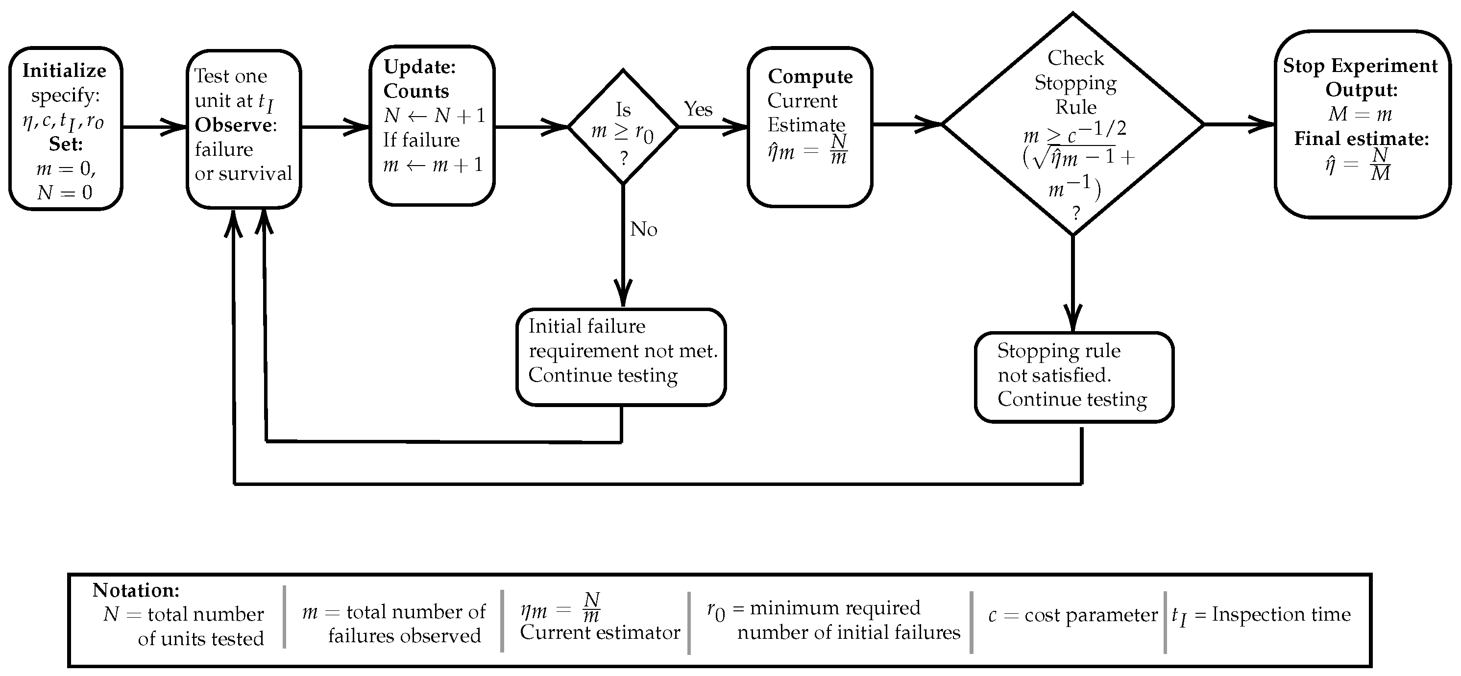
Figure 1 provides a schematic illustration of the proposed sequential one-shot testing procedure used in the simulation study. The flowchart visually summarizes the adaptive testing mechanism and stopping rule implementation, thereby clarifying the sequential decision process underlying the Monte Carlo experiments.

We summarize the results in

Table 1. Simulation results for the sequential estimation procedure with $\eta =3$, $t_I=1$, $r_0=5$, and R = 1,000,000 replications.

c	${\overline{\widehat{\mathit{\eta }}}}_{\mathit{N}}$	s.e.(${\widehat{\mathit{\eta }}}_{\mathit{N}}$)	$\overline{\mathit{M}}$	${\mathit{r}}^{*}$	$\overline{\mathit{M}}/{\mathit{r}}^{*}$	${\mathit{R}}_{\mathit{M}}\left(\mathit{c}\right)$	${\mathit{R}}_{{\mathit{r}}^{*}}\left(\mathit{c}\right)$	${\mathit{R}}_{\mathit{M}}\left(\mathit{c}\right)/{\mathit{R}}_{{\mathit{r}}^{*}}\left(\mathit{c}\right)$
0.01	2.9760	0.0006	15.22	14.14	1.0759	0.8563	0.8485	1.0091
0.005	2.9803	0.0005	21.01	20.00	1.0505	0.6041	0.6000	1.0068
0.001	2.9897	0.0004	45.75	44.72	1.0231	0.2691	0.2683	1.0030
0.0005	2.9921	0.0003	64.24	63.25	1.0157	0.1901	0.1897	1.0018
0.0001	2.9970	0.0002	142.46	141.42	1.0073	0.0850	0.0849	1.0016
0.00005	2.9976	0.0002	201.01	200.00	1.0051	0.0601	0.0600	1.0015

. Across all cost settings, the ratio $\overline{M}/r^{*}$ remains close to one, indicating that the sequential rule stops near the theoretical optimum. Likewise, the risk ratio $R_M\left(c\right)/R_{r^{*}}\left(c\right)$ remains close to one, showing that the achieved risk is nearly identical to the ideal fixed-sample benchmark. As the relative sampling cost c approaches 0, the average stopping time increases while the estimation error decreases, consistent with the first-order efficiency established in Section 3.

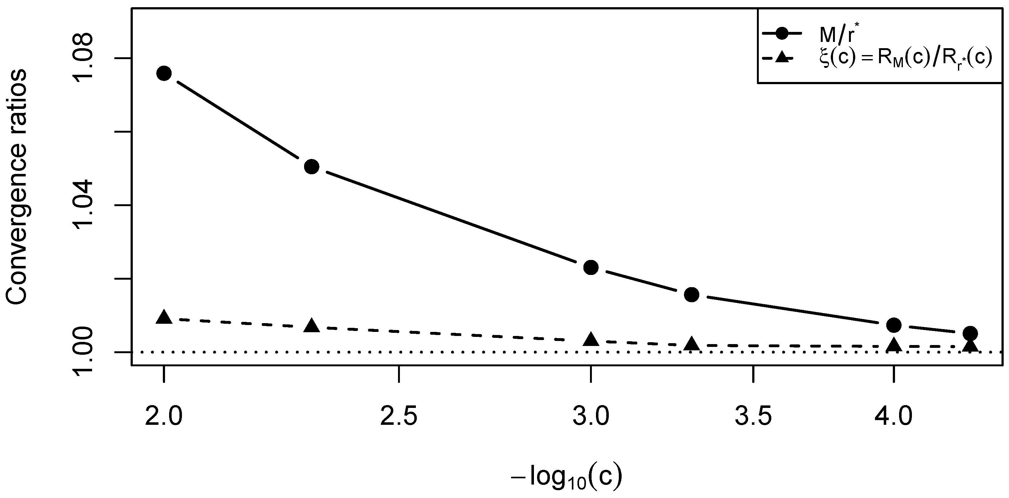
In addition, we present Figure 2, which displays the convergence of the normalized number of failures, $M/r^{*}$, and the normalized risk ratio, $\xi \left(c\right)=R\left(c\right)/R_{r^{*}}\left(c\right)$, as functions of c on a logarithmic scale. As c decreases, both quantities approach one, providing a visual confirmation of Theorems 1 and 2.

4.2. Application: Aerosol Filtration of Stored Respirators

To illustrate the practical utility of the proposed sequential framework, we construct a stockpile–reliability case study calibrated to summary results reported by Lin et al. [27]. The setting is naturally interpreted as a stockpile problem, where a large number of respirators are stored for extended periods and may degrade before use. Because only published summary statistics are available, the analysis below should be understood as an illustrative degradation-calibrated simulation study rather than a reanalysis of raw stockpile data.

The study involved five NIOSH-certified [29] N95 filtering facepiece respirator (N95FFR) models that were stockpiled for various durations in Taiwan following the SARS outbreak impact reported in Lin et al. [27]. Aerosol particles were passed through six samples from each of the five mask models under controlled laboratory conditions. The percentage of aerosol penetration was measured and compared against standardized testing criteria to evaluate the filtration performance of the masks.

From a reliability perspective, each respirator can be viewed as a one-shot device whose performance degrades over time, with failure defined as exceeding a specified penetration threshold. Since testing is destructive, only a limited number of units can be sampled from the stockpile. This naturally motivates the use of sequential estimation procedures that balance testing cost against the risk of inaccurate reliability assessment. In this context, our framework provides an efficient strategy to estimate the failure probability and certify the reliability of the stockpiled respirators under degradation.

In reliability applications for highly reliable one-shot devices, like respirators, it is common to parameterize reliability through the survival (or success) odds,

$$\omega ={\displaystyle \frac{1-p_f}{p_f}}={\displaystyle \frac{1}{p_f}}-1=\eta -1,$$

where $\eta ={\displaystyle \frac{1}{p_f}}$ is the parameter we used in the sequential estimation. Therefore, estimating the survival odds is equivalent to estimating $\eta$, the two quantities differing only by a constant shift. Hence, we develop the sequential procedure in terms of $\eta$, and the corresponding survival odds can be recovered immediately as $\eta -1$.

4.2.1. Degradation-Model Calibration

We used plot digitization to extract the approximate mean and standard deviation of the penetration levels from a clustered bar chart with error bars, as in Lin et al. [27]. The mean penetration level (%) of the 3M-8210 model and its standard error are approximately 0.212 and 0.087 at Year 3, and 0.399 and 0.218 at Year 7, respectively.

The ideal aerosol filtration loss should be 0, but to make it realistic, we assume that the initial filtration loss is $\kappa$ and the further aerosol penetration percentage $D_l\left(\tau \right)$ follows a gamma degradation model $(\alpha \tau ,\beta )$. Using the approximated data, we obtain the parameters of the gamma degradation model as: $\alpha =0.078,\beta =1.673,$ and $\kappa =0.072$. Because failure is defined by threshold exceedance, the implied failure probability at inspection time $t_I$ is

$$p_f\left(t_I\right)=\mathrm{Pr}\{D_l\left(t_I\right)+\kappa \ge D_{th}\}=1-F_{\mathrm{\Gamma }}(D_{th}-\kappa ;\alpha t_I,\beta ),$$

where $F_{\mathrm{\Gamma }}(D_{th};\alpha t_I,\beta )={\int }_0^{D_{th}}{\displaystyle \frac{{\beta }^{\alpha t_I}}{\mathrm{\Gamma }\left(\alpha t_I\right)}}{x}^{\alpha t_I-1}\exp (-\beta x)dx$ denotes the gamma cumulative distribution function. The sequential procedure is then applied with

$${\eta }_{t_I}={\displaystyle \frac{1}{p_f\left(t_I\right)}}.$$

The primary objective here is to certify whether a specific stockpile complies with an internal safety threshold $D_{th}=2\%$. This choice is intentionally more conservative than the 5% NIOSH particulate-penetration criterion for N95 respirators and is used here to illustrate how the sequential procedure can accommodate stricter decision thresholds. At the inspection time $t_I=5$ years, we therefore set

$$p_f\left(5\right)=P(D_l\left(5\right)+\kappa \ge 2\%)=0.0074283\Rightarrow {\eta }_{t_I=5}={\displaystyle \frac{1}{p_f\left(5\right)}}=134.62,$$

where ${\eta }_{t_I=5}={\displaystyle \frac{1}{p_f\left(5\right)}}$ is the reciprocal of true failure probability at Year 5.

Now, we optimize the loss function to balance the physical testing cost against the financial liability of estimation error. For modeling the monetary loss function, there are two parts: one for the cost of destroying a mask for testing, and one for the cost of incorrect estimation. The monetary liability cost incurred for inaccurately estimating $\eta$ is very high for the hospital administration since it directly affects the reliability assessment of the stockpile, leading to health hazards. So, the monetary loss function for our proposed sequential test can be modeled as

$$L_{\$}=C_l{(\widehat{\eta }-{\eta }_{t_I=5})}^2+C_{\mathrm{test}}N,$$

(29)

$C_{\mathrm{test}}$ represents the direct cost to destructively test one N95 mask, say $10.00 encompassing the unit price and laboratory labor, and $C_l$ is the monetary liability of inaccurate estimation of ${\eta }_{t_I=5}$ say a penalty of $10,000 per squared error.

To provide the utility of our proposed sequential testing, we use the standard estimation method to compute the odds estimate. Then compare the number of items destroyed to certify the stockpile for safe use, and the loss (29).

4.2.2. Sequential Design

We use our sequential testing method to obtain the optimal number of masks needed to test to certify that the batch is compliant with the safety threshold. The loss function can be simplified to

$$L_N={\displaystyle \frac{L_{\$}}{C_l}}={(\widehat{\eta }-{\eta }_{t_I=5})}^2+cN,\mathrm{where}c={\displaystyle \frac{C_{\mathrm{test}}}{C_l}}=0.001.$$

This small cost parameter ($c=0.001$) mathematically forces the sequential stopping rule to heavily prioritize statistical precision. The stopping boundary continuously updates based on the empirical estimate rather than static assumptions.

Since the loss function $L_N$ matches the theoretical loss function in Section 2, we apply the sequential stopping rule to each simulated batch and record the resulting stopping sample size, estimator, and loss. Repeating this procedure over 10,000 Monte Carlo runs yields the summary results reported in

Table 2. Sequential-design results for the stockpile case study. Entries are Monte Carlo means, with Monte Carlo standard errors after the ± sign based on 10,000 replications.

Estimated $\mathit{\eta }$ ($\widehat{\mathit{\eta }}$)	Average Stopping Sample Size ($\overline{\mathit{N}}$)	Average Estimated Loss ($ Thousands)
$134.38\pm 0.0060$	49,216 ± 0.1728	$979\pm 0.2186$

. Additional results for other N95 respirator models in Lin et al. [27] are provided in the Appendix A.

4.2.3. Fixed-Sample Benchmark

For the testing procedure with a fixed-sample size, the true failure probability is unknown at the design stage. Consequently, the conventional approach must rely on an assumed operational baseline for the failure probability, denoted by $p_{f_a}$, or equivalently, the assumed ${\eta }_a={\displaystyle \frac{1}{p_{f_a}}}$. Researchers can obtain the assumed values from pilot studies or expert experience, and use them for determining the sample size, which may differ from the true failure probability $p_{f,\mathrm{true}}$.

The loss function (29) is minimized when the squared errors of the estimator, ${(\widehat{\eta }-{\eta }_{\mathrm{true}})}^2$, are small. Assuming $\widehat{\eta }$ is approximately unbiased, the optimal sample size $N^{*}$ is obtained by minimizing the trade-off between estimation uncertainty ($\mathrm{Var}\left(\widehat{\eta }\right)$) and testing cost. If the number of tested units, N, is fixed, the number of failed units follows $R\sim \mathrm{Bin}(N,p_{f_a})$. Then,

$$\mathrm{Var}\left({\widehat{p}}_f\right)=\mathrm{Var}\left({\displaystyle \frac{R}{N}}\right)={\displaystyle \frac{p_{f_a}(1-p_{f_a})}{N}}.$$

Since $\widehat{\eta }={\displaystyle \frac{1}{{\widehat{p}}_f}}$ using the Delta method, we obtain

$$\mathrm{Var}\left(\widehat{\eta }\right)={\left({\displaystyle \frac{\partial \widehat{\eta }}{\partial {\widehat{p}}_f}}\right)}^2\times \mathrm{Var}\left(\widehat{p_f}\right)={\displaystyle \frac{1-p_{f_a}}{N{p}_{f_a}^3}}={\displaystyle \frac{{\eta }_a^2({\eta }_a-1)}{N}}.$$

Thus, the risk function based on the fixed-sample size, N is

$$R_N={\displaystyle \frac{C_l{\eta }_a^2({\eta }_a-1)}{N}}+C_{\mathrm{test}}N.$$

To find $N=N_{\mathrm{conv}}^{*}$ that minimize $R_N$, we solve

$${\displaystyle \frac{\partial R_N}{\partial N}}{|}_{N=N_{\mathrm{conv}}^{*}}=0,$$

which gives

$$N_{\mathrm{conv}}^{*}=\sqrt{{\displaystyle \frac{C_l{\eta }_a^2({\eta }_a-1)}{C_{\mathrm{test}}}}}.$$

Finally, the risk function of this design is evaluated with respect to the true ${\eta }_{t_I=5}$:

$$R_{N_{\mathrm{conv}}^{*}}=C_l{(\widehat{\eta }-{\eta }_{t_I=5})}^2+C_{\mathrm{test}}{N}_{\mathrm{conv}}^{*}.$$

Since the assumed estimates are different from the true value, ${\eta }_a\ne {\eta }_{t_I=5}$, the conventional design may yield suboptimal performance relative to the true system behavior.

4.2.4. Simulation Comparison

For the conventional fixed-sample design, the true failure probability at the inspection time is typically unknown at the planning stage. Therefore, the sample size is determined using a planning value $p_{f_a}$, or equivalently ${\eta }_a=1/p_{f_a}$, obtained from pilot data, prior degradation studies, or engineering judgment. If this planning value differs from the true value, that is, ${\eta }_a\ne {\eta }_{t_I=5}$, the resulting fixed-sample design may no longer minimize the risk under the actual system behavior.

In our study, we consider two baseline values for the fixed-sample design, namely ${\eta }_a=100$ and ${\eta }_a=200$, corresponding to failure probabilities of $1\%$ and $0.5\%$, respectively, while the true reciprocal failure probability is $\eta =134.62$. We acknowledge that the sequential procedure benefits from adaptively incorporating observed data, whereas the conventional design relies on a prespecified baseline value. This reflects a practical distinction between the two approaches: fixed-sample procedures are inherently sensitive to misspecification of the assumed failure probability, while sequential methods update the sampling process through continued observation.

We conduct 10,000 simulation runs for both the sequential and conventional approaches. The resulting estimates, optimal sample sizes, and associated losses are summarized in Table 2 and

Table 3. Conventional fixed-sample design results for the stockpile case study under two assumed baseline values ${\eta }_a$. Entries are Monte Carlo means, with Monte Carlo standard errors after the ± sign, based on 10,000 replications.

Assumed $\mathit{\eta }$ (${\mathit{\eta }}_{\mathit{a}}$)	Estimated $\mathit{\eta }$ ($\widehat{\mathit{\eta }}$)	Optimum Fixed Sample Size (N)	Average Estimated Loss ($ Thousands)
200	$134.80\pm 0.0046$	89,219	$1178\pm 0.1240$
100	$135.26\pm 0.0077$	31,464	$1122\pm 0.3800$

.

The comparison results indicate that the proposed sequential estimation procedure achieves competitive and, in many cases, lower overall monetary loss than the conventional fixed-sample approach under the considered settings. The conventional method determines the sample size using pre-specified baseline failure odds, whereas the sequential procedure adaptively updates the required number of tested units using the observed data. In practice, the true failure odds are typically unknown in advance, so fixed-sample designs may be sensitive to misspecification of the assumed baseline values. The sequential framework partially mitigates this issue through adaptive sampling, leading to an improved balance between testing cost and estimation accuracy in many scenarios. Although the magnitude of improvement varies across settings, the results suggest that the proposed sequential procedure provides an effective and practically attractive alternative for stockpile reliability applications, where destructive testing costs and conservation of testing resources are critically important considerations.

5. Discussion and Concluding Remarks

We developed a sequential estimation framework for one-shot devices observed through binary current-status data at a fixed inspection time. Building on the sequential censoring ideas of Hu et al. [28], we adapted the methodology to destructive one-shot testing, where each tested unit is consumed, and efficient use of stockpiled items is therefore essential. The proposed procedure balances estimation error against testing cost through a risk-based stopping rule and leads to a random sample size with a negative-binomial structure. This formulation is particularly appealing in stockpile reliability monitoring, where failures are rare, testing is destructive, and unnecessary sampling directly reduces the remaining usable inventory.

The theoretical results show that the proposed procedure is first-order efficient relative to the optimal fixed-sample benchmark. In particular, the stopping rule asymptotically attains the same risk level as the ideal design that would be chosen if the true failure probability were known in advance. The simulation study further confirms that both the achieved stopping time and the resulting risk remain close to their theoretical targets over a wide range of cost settings. These findings support the practical use of the procedure as a resource-efficient alternative to conventional fixed-sample designs.

The proposed framework is formulated in terms of the inspection-time failure probability

$$p_f=F(t_I;\theta ),\eta ={\displaystyle \frac{1}{p_f}},$$

and is therefore not restricted to the exponential model alone. In principle, it can be used with any one-parameter lifetime distribution for which the inspection-time failure probability is well defined. The exponential model is adopted in this paper because it yields explicit expressions for the mean lifetime, survival function, and mission-time reliability, thereby allowing the sequential procedure to be developed in a transparent form. The stockpile case study further illustrates how the procedure can be combined with a degradation-based calibration when only limited destructive testing is feasible.

At the same time, several limitations should be acknowledged. First, although the sequential stopping logic is distributionally broader, the explicit reliability and mean-lifetime calculations in this paper rely on the exponential model. Second, the respirator example is an illustrative degradation-calibrated simulation based on published summary statistics rather than a direct reanalysis of raw stockpile data. Third, the current formulation assumes a homogeneous stockpile and a fixed inspection time, whereas real stockpiles may exhibit batch effects, age heterogeneity, or operationally constrained inspection schedules.

These limitations suggest several concrete directions for future research. One important extension is to develop analogous sequential procedures for multi-parameter lifetime models, such as the Weibull and lognormal distributions, where the inspection-time failure probability depends on more than one unknown parameter. A second direction is to incorporate finite-stockpile constraints directly into the stopping rule, so that the procedure explicitly accounts for the remaining inventory and not only the per-test sampling cost. A third direction is to integrate degradation information and binary current-status outcomes in a unified sequential framework, so that indirect health indicators and destructive pass/fail tests can be used jointly. It would also be valuable to study robustness under model misspecification, especially when the assumed lifetime model is only an approximation to the actual storage-failure mechanism. Additional extensions include allowing multiple inspection times, accounting for imperfect classification in pass/fail testing, and developing Bayesian or empirical-Bayes versions of the procedure for situations in which prior engineering information is available. Another practically relevant extension is to allow multiple inspection times or imperfect pass/fail classification, both of which arise naturally in stockpile surveillance programs and would require modification of the current stopping rule and risk analysis.

Overall, the proposed sequential framework provides a practically useful and theoretically justified tool for reliability monitoring in stockpile environments where failures are rare and destructive testing is costly. It offers a principled way to reduce unnecessary testing while preserving statistical precision, and it opens a path toward more realistic sequential monitoring procedures for complex one-shot systems in future work.

References

1. Sen, P.K. On time-sequential point estimation of the mean of an exponential distribution. Commun. Stat.-Theory Methods 1980, 9, 27–38. [Google Scholar] [CrossRef]
2. Stadje, W. A sequential estimation procedure for the parameter of an exponential distribution. Statistics 1990, 21, 239–250. [Google Scholar] [CrossRef]
3. Mukhopadhyay, N. Second-order approximations in the time-sequential point estimation methodologies for the mean of an exponential distribution. Seq. Anal. 1995, 14, 133–142. [Google Scholar] [CrossRef]
4. Mukhopadhyay, N.; Chattopadhyay, S. Sequential methodologies for comparing exponential mean survival times. Seq. Anal. 1991, 10, 139–148. [Google Scholar] [CrossRef]
5. Mukhopadhyay, N.; Pepe, W. Exact bounded risk estimation when the terminal sample size and estimator are dependent: The exponential case. Seq. Anal. 2006, 25, 85–101. [Google Scholar] [CrossRef]
6. Mukhopadhyay, N.; Khariton, Y. Minimum risk point estimation (MRPE) of the mean in an exponential distribution under powered absolute error loss. Seq. Anal. 2020, 39, 241–268. [Google Scholar] [CrossRef]
7. Mukhopadhyay, N.; Li, J. Purely sequential minimum risk point estimation (MRPE) for a survival function in an exponential distribution. J. Stat. Theory Pract. 2022, 16, 50. [Google Scholar] [CrossRef]
8. Zhu, T. Reliability estimation for two-parameter Weibull distribution under block censoring. Reliab. Eng. Syst. Saf. 2020, 203, 107071. [Google Scholar] [CrossRef]
9. Gardiner, J.C.; Susarla, V. Sequential estimation of the mean survival time under random censorship. Commun. Stat. Seq. Anal. 1983, 2, 201–223. [Google Scholar] [CrossRef]
10. Gardiner, J.C.; Susarla, V.; Ryzin, J.V. Time sequential estimation of the exponential mean under random withdraws. Ann. Stat. 1986, 14, 607–618. [Google Scholar] [CrossRef]
11. Aras, G. Sequential estimation of the mean exponential survival time under random censoring. J. Stat. Plan. Inference 1987, 16, 147–158. [Google Scholar] [CrossRef]
12. Aras, G. Second order sequential estimation of the mean exponential survival time under random censoring. J. Stat. Plan. Inference 1989, 21, 3–17. [Google Scholar] [CrossRef]
13. Anscombe, F.J. Large-sample theory of sequential estimation. Math. Proc. Camb. Philos. Soc. 1952, 48, 600–607. [Google Scholar] [CrossRef]
14. Chow, Y.S.; Robbins, H. On the asymptotic theory of fixed-width sequential confidence intervals for the mean. Ann. Math. Stat. 1965, 36, 457–462. [Google Scholar] [CrossRef]
15. Ghosh, M.; Mukhopadhyay, N. On two fundamental problems of sequential estimation. Sankhya Ser. B 1976, 38, 203–218. [Google Scholar]
16. Starr, N. On the asymptotic efficiency of a sequential procedure for estimating the mean. Ann. Math. Stat. 1966, 37, 1173–1185. [Google Scholar] [CrossRef]
17. Zhang, Z.; Si, X.; Hu, C.; Kong, X. Degradation modeling–based remaining useful life estimation: A review. Proc. Inst. Mech. Eng. Part O J. Risk Reliab. 2015, 229, 343–355. [Google Scholar] [CrossRef]
18. Houlding, B.; Coolen, F.P.A. Sequential adaptive utility decision making for system failure correction. Proc. Inst. Mech. Eng. Part O J. Risk Reliab. 2007, 221, 285–295. [Google Scholar] [CrossRef]
19. Balakrishnan, N.; Ling, M.H.; So, H.Y. Accelerated Life Testing of One-shot Devices: Data Collection and Analysis; Wiley: Hoboken, NJ, USA, 2021. [Google Scholar]
20. U.S. Navy. Production Issue with Ejection Seat Cartridge Actuated Devices (CAD) Necessitates Aircraft Inspections Across Fleet. 2022. Available online: https://www.navy.mil/Press-Office/Press-Releases/display-pressreleases/Article/3105635/production-issue-with-ejection-seat-cartridge-actuated-devices-cad-necessitates/ (accessed on 1 January 2025).
21. Vander Wiel, S.A.; Wilson, A.G.; Graves, T.L.; Reese, C.S. A Random Onset Model for Degradation of High-Reliability Systems. Technometrics 2011, 53, 163–172. [Google Scholar] [CrossRef]
22. Si, X.S.; Wang, W.; Hu, C.H.; Zhou, D.H. Remaining Useful Life Estimation—A Review on the Statistical Data Driven Approaches. Eur. J. Oper. Res. 2011, 213, 1–14. [Google Scholar] [CrossRef]
23. Elsayed, E.A. Reliability Engineering, 2nd ed.; John Wiley & Sons: Hoboken, NJ, USA, 2012. [Google Scholar]
24. National Research Council. Evaluation of Quantification of Margins and Uncertainties Methodology for Assessing and Certifying the Reliability of the Nuclear Stockpile; The National Academies Press: Washington, DC, USA, 2009. [CrossRef]
25. Chen, Y.; Zhang, Q.; Cai, Z.; Wang, L. Storage Reliability Assessment Model Based on Competition Failure of Multi-Components in Missile. J. Syst. Eng. Electron. 2017, 28, 606–616. [Google Scholar] [CrossRef]
26. Bergman, M.S.; Viscusi, D.J.; Zhuang, Z.; Palmiero, A.J.; Powell, J.B.; Shaffer, R.E. Impact of Multiple Consecutive Donnings on Filtering Facepiece Respirator Fit. Am. J. Infect. Control 2012, 40, 375–380. [Google Scholar] [CrossRef]
27. Lin, T.H.; Tseng, C.C.; Huang, Y.L.; Lin, H.C.; Lai, C.Y.; Lee, S.A. Effectiveness of N95 facepiece respirators in filtering aerosol following storage and sterilization. Aerosol Air Qual. Res. 2020, 20, 833–843. [Google Scholar] [CrossRef]
28. Hu, J.; So, H.Y.; Zhuang, Y. Estimation of the mean exponential survival time under a sequential censoring scheme. J. Appl. Stat. 2025, 52, 669–686. [Google Scholar] [CrossRef] [PubMed]
29. NIOSH. Approval of Respiratory Protective Devices; National Institute for Occupational Safety and Health: Washington, DC, USA, 1995; Volume 42, pp. 505–569.
Figure 1. A flowchart illustrating the proposed sequential one-shot testing procedure for stockpile monitoring and the adaptive stopping mechanism used in the simulation study.
Mathematics 14 01858 g001
Figure 2. Convergence of the normalized stopping and risk quantities as the relative cost parameter c 0 . The ratio M / r * approaches one, supporting Theorem 1, while the risk efficiency ratio ξ ( c ) = R M ( c ) / R r * ( c ) approaches one, supporting Theorem 2.
Mathematics 14 01858 g002