Frequency–Severity Asymmetry and Regime-Based Forecasting of Operational Downtime in Continuous Material-Handling Systems

Abstract

Operational failures in continuous material-handling systems are usually evaluated through failure counts; however, failure frequency alone may underestimate the true operational burden when downtime severity is unevenly distributed across devices and fault mechanisms. This study develops an integrated statistical framework for analysing operational failures and downtime in a continuous material-handling and technological transport process. The empirical dataset consists of 6605 anonymised failure events recorded between 2017 and 2025, covering 108 monthly observations, three technological device categories, and 42 classified fault types. The methodology combines frequency–severity analysis, inferential testing, time-series forecasting, and cluster-based identification of monthly operating regimes. The results show a strong disproportionality between failure frequency and downtime burden. Conveyor belts accounted for 51.40% of all failures but generated 83.22% of total downtime, confirming their dominant role in system-level operational losses. Several fault types, including Belt Slip, Off-Track Belt, Tear, Motor Failure, and Transfer Chute, also exhibited high downtime severity despite lower occurrence frequency. Inferential testing confirmed statistically significant and operationally meaningful differences in downtime severity across machine categories, whereas the calendar month was not a significant determinant of monthly failure counts or total downtime. Among the candidate forecasting models, Seasonal and Trend decomposition using Loess combined with exponential smoothing (STL-ETS) achieved the best holdout performance for both failure counts and total downtime. Cluster analysis further identified six interpretable monthly operating regimes differing in failure intensity, downtime burden, equipment involvement, fault-type composition, and temporal growth dynamics. The study contributes to downtime-oriented maintenance analytics by demonstrating that operational risk should be assessed through combined frequency–severity and regime-based perspectives rather than through aggregate failure counts alone.

1. Introduction

Continuous material-handling and technological transport systems are critical for production continuity, system availability, maintenance planning, and operational efficiency. Failures in such systems are not only isolated technical interruptions; they cause downtime, increase maintenance demand, reduce process stability, and may affect the performance of downstream operations. Therefore, a reliability assessment should not be based solely on the number of recorded failures but also on the consequences of the downtime they cause.

Although predictive maintenance and industrial analytics have advanced significantly, an important research problem remains unresolved: failure frequency and downtime severity are not necessarily proportional. Some faults may occur frequently but cause limited downtime, whereas less frequent failures may generate disproportionately high operational losses. In addition, failure behaviour may vary over time, giving rise to different operating regimes rather than following a stable or homogeneous process.

This study analyses anonymised operational failure records from a continuous material-handling and technological transport process covering the period 2017–2025. The dataset includes 6605 failure events, three technological device categories, 42 classified fault types, and 108 monthly observations. The aim is to develop an integrated analytical framework that combines frequency–severity assessment, inferential testing, time-series forecasting, and cluster-based identification of monthly operating regimes.

The study is guided by the following research questions:

RQ1. 

How is downtime burden distributed across technological devices and fault types, and is it proportional to failure frequency?

RQ2. 

Do machine categories differ significantly in downtime severity?

RQ3. 

What temporal patterns characterise annual and monthly failure occurrence and downtime, and can they be forecasted using time-series models?

RQ4. 

Can monthly operating states be grouped into interpretable regimes that differ in failure intensity, downtime burden, equipment structure, fault composition, and temporal dynamics?

The contribution of the study lies in moving beyond descriptive failure counts toward a multidimensional assessment of operational risk. By integrating downtime severity, statistical testing, forecasting, and clustering, the study provides a framework for identifying high-risk devices, critical fault mechanisms, and operating regimes relevant for maintenance prioritisation and decision support.

2. Literature Review

2.1. Predictive Maintenance and Data-Driven Failure Modelling

Predictive maintenance research has shifted from reactive failure correction to data-driven anticipation of operational disruptions, with failures increasingly interpreted as time-dependent, technically embedded processes. IoT-, cloud-, and machine learning-based conveyor monitoring can detect failure indicators before they lead to critical downtime [1], while intelligent machine learning approaches support Total Productive Maintenance and reduce unplanned stoppages [2]. Reviews of industrial time-series forecasting emphasise the need to capture trend, seasonality, irregular fluctuations, and production-specific temporal structures [3]. Risk-based inspection, ARIMA models, and neural-network forecasting further show that reliability analysis should consider both failure probability and operational consequence [4,5]. Recent applications of random forests, digital twins, real-time maintenance management, multiclass anomaly detection, and Weibull degradation modelling extend this logic toward integrated predictive-maintenance systems [6,7,8,9,10]. However, the question of whether frequent failures are also the dominant source of downtime burden remains only partly addressed.

2.2. Conveyor Systems, Equipment Criticality, and Damage Mechanisms

Conveyor systems represent a specific reliability domain because their failures can interrupt entire material-flow chains and generate secondary operational losses. Empirical studies on rubber conveyor-belt reliability confirm their importance for production continuity [11], while reviews of industrial condition monitoring emphasise sensor-based diagnostics, automated data processing, and model interpretability [12]. Digital transformation research identifies IoT, cloud architectures, edge computing, and machine learning as key pillars of conveyor-belt predictive maintenance [13]. Conveyor-motor fault prediction, roller-condition monitoring, time-series analytics, event-sequence modelling, machine learning adoption, integrated decision-making, and uncertainty assessment collectively indicate that conveyor failures exhibit dynamic, multi-component characteristics [14,15,16,17,18,19,20]. This supports the need to examine failure occurrence alongside downtime consequences and the technical context.

2.3. Failure Forecasting, Downtime Prediction, and Operational Losses

Failure and downtime prediction are closely linked to time-series modelling because industrial failures often occur in episodes, local peaks, and temporally uneven clusters rather than uniformly. Hybrid XGB-metaheuristic models improved time-to-failure prediction in mining machinery [21], while conveyor-belt wear models showed that historical condition data can be transformed into degradation indicators [22]. Machine learning and deep learning models have been used to minimise manufacturing downtime [23], and ARMA-based approaches remain relevant for fault-event prediction [24]. AI-based conveyor deterioration models further connect degradation forecasting with maintenance planning [25]. Similar predictive logic has been confirmed through IoT sensor data, rubber-textile belt failure classification, hybrid CNN-LSTM architectures, expert systems, Taguchi-based diagnostics, and scalable BigDL forecasting models [26,27,28,29,30]. These studies provide a strong predictive basis, but they rarely combine forecasting with device-level inference and multivariate operating-regime identification.

2.4. Frequency–Severity Asymmetry and Fault-Type Structure

A central issue in maintenance analytics is that the number of failures is not necessarily a reliable measure of operational burden. Reviews of conveyor-belt damage show that failures arise from the interaction of mechanical, operational, and environmental factors [31], while idler-monitoring research confirms that local component degradation may generate system-level constraints [32]. Studies of rolling-stock systems, IT infrastructure, and predictive scheduling similarly show that failures must be prioritised by consequence, not merely detected [33,34,35]. Downtime-oriented research strengthens this argument by treating outage duration as an analytical variable in its own right rather than as a simple derivative of failure frequency [36]. Time-based failure prediction in multi-machine systems, production-line downtime analytics, throughput bottleneck modelling, and belt-conveyor failure-pattern analysis all indicate that frequency, duration, and system-level consequence may diverge substantially [37,38,39,40]. This literature therefore provides a clear basis for examining the mismatch between failure share and downtime burden.

2.5. Energy Sustainability, Operational Research, and Maintenance Decision-Making

Operational reliability is also relevant to energy efficiency and sustainability, as unplanned downtime, repeated start-ups, and unstable operating states can increase resource consumption and reduce process continuity. In this context, maintenance analytics can support not only technical reliability but also broader operational decision-making. Previous studies on energy-system indicators, equipment life-cycle models, prescriptive maintenance, and Industry 4.0-based maintenance management show that mathematically grounded reliability assessment can contribute to more efficient equipment use, better planning, and risk-informed maintenance prioritisation [41,42,43,44,45,46,47]. In the present study, this perspective is used only as a supporting context; the core analytical focus remains on failure frequency, downtime severity, forecasting, and operating-regime identification.

2.6. Multivariate Operating Regimes and the Research Gap

Recent literature suggests that failure behaviour should be treated as a multivariate process encompassing frequency, severity, equipment type, fault type, and temporal dynamics. Time-series models for construction equipment, multivariate industrial time series, Cox models based on recurring failure signatures, log- and ticket-based outage prediction, and reliability assessment of bulk-solid carriers indicate that operational failures may manifest as structured regimes rather than isolated events [48,49,50,51,52]. Further studies highlight technical interventions, interpretable models, digital twins, data fusion, conveyor-core damage trajectories, logistics automation, pipe-conveyor failures, and early idler-fault detection [53,54,55,56,57,58,59,60,61]. Evidence from related systems, including automotive maintenance, long-sequence prediction, photovoltaic degradation forecasting, downtime-duration modelling, FMEA-based reliability assessment, optimised conveyor-maintenance strategies, and statistical decision thresholds, confirms the need for an integrated analytical framework [62,63,64,65,66,67,68,69,70,71].

Overall, the literature has advanced failure prediction, conveyor diagnostics, time-series modelling, and damage classification, but it still insufficiently connects failure frequency, downtime severity, and the structure of monthly operating states. The present study addresses this gap by analysing operational failures as a multidimensional, temporally structured, and downtime-differentiated process. Conceptually, the proposed framework links five analytical dimensions of operational reliability: failure frequency, downtime severity, equipment category, fault-type structure, and temporal dynamics. These dimensions are operationalised through device- and fault-level burden indicators, inferential tests of downtime differences, time-series forecasts of monthly failure counts and downtime, and cluster-based identification of monthly operating regimes. This structure allows the study to examine not only how often failures occur, but also where downtime burden is concentrated and how monthly operating states vary over time.

3. Materials and Methods

3.1. Methodological Framework, Data Origin, and Research Hypotheses

The empirical basis of the study consists of anonymised secondary operational records obtained from long-term monitoring of a continuous material-handling and technological transport process. The records correspond to real downtime events registered during routine operation and include the event timestamp, downtime duration, affected equipment category, and standardised technical fault type. The dataset was not generated through simulation or laboratory experimentation; it reflects operational data collected as part of regular maintenance, dispatching, and production-continuity monitoring. To preserve confidentiality, the analysis treats the records as an anonymised operational failure dataset and focuses on failure occurrence, downtime burden, forecasting performance, and monthly operating regimes.

Data provenance and downtime definition. The analysed records were obtained from an internal operational information system used for registering technological-unit activities, failures, stoppages, and production-related events. Each registered activity contains the affected device, start time, end time, duration, activity code, activity description, and operational notes when available. The source system distinguishes primary activities, which represent the immediate reason for interrupting or limiting normal operation, from secondary activities, which document other relevant operational actions during the shift. The operational day follows the continuous-shift regime and is recorded from 06:00 to 06:00 of the following day. In this study, downtime was defined as the registered duration between the start and end of a failure-related or stoppage-related event. Very short interruptions were included only when formally registered with a corresponding activity code; unregistered micro-stoppages were not included in the analysis. Before statistical processing, site-specific identifiers, personnel information, detailed equipment labels, and company-specific operational references were removed or aggregated.

All preprocessing, variable harmonisation, statistical computations, model estimation, validation procedures, and graphical outputs were performed in RStudio using R version 4.5.2. The analytical workflow consisted of data standardisation, temporal aggregation, device- and fault-level burden assessment, inferential testing, time-series forecasting, and multivariate cluster-based regime identification.

Let the event-level failure dataset be denoted as:

$$\mathcal{D}=\left\{\right(t_i,m_i,f_i,d_i){\}}_{i = 1}^N,$$

(1)

where $t_i$ is the timestamp of the $i$-th failure event, $m_i\in \mathcal{M}$ denotes the technological device category, $f_i\in \mathcal{F}$ represents the standardised fault type, and $d_i > 0$ is the downtime duration measured in minutes. The methodological design distinguishes two complementary dimensions of operational disruption: the occurrence frequency of failures and their time-related severity.

Based on this framework, two analytical research hypotheses were formulated:

H1. 

The operational downtime burden is not proportional to failure frequency across technological device and fault-type categories; instead, it is expected to be concentrated in a limited set of high-severity components and fault mechanisms.

H2. 

Monthly failure behaviour can be represented by distinct operating regimes that differ not only in failure intensity and downtime burden, but also in the joint structure of equipment involvement, fault-type composition, and temporal growth dynamics.

3.2. Data Source and Analytical Sample

Before conducting the statistical modelling procedures, the analytical dataset was systematically examined for temporal coverage, the number of recorded failure events, the structure of technological device categories, and data completeness. This step is methodologically important because the quality of the input dataset directly affects the reliability of subsequent frequency-based, temporal, inferential, and predictive analyses. As shown in

Table 1. Overview of the analytical dataset and basic descriptive indicators. Source: own processing in RStudio, R version 4.5.2.

Indicator	Value
Start of the analytical period	1 January 2017
End of the analytical period	31 December 2025
Number of calendar years	9
Number of monthly observations	108
Number of failure events	6605
Number of device categories	3
Number of classified fault types	42
Total downtime (min)	977,890
Total downtime (hours)	16,298.17
Mean downtime per failure event (min)	148.0530
Median downtime per failure event (min)	201.0000

, the final analytical dataset covers the nine-year period from 2017 to 2025 and comprises 6605 recorded failure events after the exclusion of incomplete observations with missing indicator values. Total downtime reached 977,890 min, corresponding to 16,298.17 h of technological unavailability. This magnitude confirms the operational relevance of the analysed problem and justifies the application of more advanced analytical procedures focused not only on failure frequency but also on downtime severity.

For each monthly period, $\tau$, two primary response variables were constructed: monthly failure count and monthly total downtime. These variables were defined as:

$$Y_{\tau } = {\displaystyle \sum _{i = 1}^N}\mathbf{1}(t_i\in \tau ),D_{\tau } = \sum _{i:t_i\in \tau }{d}_i,$$

(2)

where $\mathbf{1}(·)$is the indicator function. The variable $Y_{\tau }$ captures the frequency dimension of operational disruptions, whereas $D_{\tau }$ expresses the cumulative downtime burden within a given month.

3.3. Device Categories and Operational Burden Structure

The distribution of operational burden across technological devices reveals a substantial imbalance between device categories. As reported in

Table 2. Frequency–severity burden of technological devices. Source: own processing in RStudio, R version 4.5.2.

Indicator	P―Conveyor Belt	R―Excavator	Z―Stacker
Number of failure events	3395	2710	500
Share of failure events (%)	51.4005	41.0295	7.570
Total downtime (min)	813,830.0000	133,142.0000	30,918.00
Share of total downtime (%)	83.2231	13.6152	3.1617
Mean downtime (min)	239.7143	49.1299	61.8360
Median downtime (min)	253.0000	55.0000	78.5000
90th percentile of downtime (min)	268.0000	77.0000	101.0000
Severity–frequency index	123.2142	20.1578	4.6810

, conveyor belts are the dominant source of operational burden, accounting for 51.40% of all failure events and up to 83.22% of total downtime. This divergence between the frequency share and the downtime share indicates that conveyor belts are not only the most frequent source of failures but also the most severe contributor to time-related operational losses. Excavators account for 41.03% of all failures but only 13.62% of total downtime, suggesting a different failure profile characterised by relatively high occurrence frequency but lower average downtime intensity. Stackers show the lowest overall burden and therefore represent a less dominant segment in terms of system-level operational risk.

Due to confidentiality restrictions, the analysis was conducted at the level of functional equipment categories rather than at the level of identifiable machine models, exact capacities, service age, or site-specific deployment roles. The categories, therefore, represent aggregated technological functions within the material-handling process. This level of aggregation is suitable for identifying broad differences in failure frequency and downtime burden, but it does not allow conclusions about the reliability of individual equipment models or specific units.

For each device category, m, the relative share of failure events, the relative share of total downtime, and the severity–frequency index (SFI) were calculated as:

$$p_m^{\left(Y\right)} = {\displaystyle \frac{N_m}{N}}, { p}_m^{\left(D\right)} = {\displaystyle \frac{\sum _{i:m_i = m}{d}_i}{{\displaystyle {\sum }_{i = 1}^N}{d}_i}}, {SFI}_m = p_m^{\left(Y\right)}·{\bar{d}}_m, {\bar{d}}_m = {\displaystyle \frac{1}{N_m}}\sum _{i:m_i = m}{d}_i.$$

(3)

Here, $N_m$ denotes the number of failures associated with device category $m$, $p_m^{\left(Y\right)}$ is the failure share, $p_m^{\left(D\right)}$ is the downtime share, and ${\bar{d}}_m$ is the mean downtime per failure event. The severity–frequency index was used to identify equipment categories that combine high failure occurrence with substantial downtime severity. The severity–frequency index (SFI) was used solely as a descriptive prioritisation indicator, not as a standalone measure of equipment criticality. Because the index combines failure share with mean downtime, it may be sensitive to high average downtime values in categories with few observations. Therefore, SFI values were interpreted together with the number of failures, downtime share, median downtime, and the 90th percentile of downtime. This combined interpretation reduces the risk of overemphasising categories with high severity but limited empirical support.

3.4. Data Completeness and Preprocessing

Data completeness was assessed to verify whether missing values could substantially affect subsequent statistical and predictive procedures. As shown in

Table 3. Variables with the highest proportion of missing values. Source: own processing in RStudio, R version 4.5.2.

Variable	Missing Count	Missing Share (%)
Interarrival time between failures by fault type	44	0.6618
Interarrival time between failures by device category	5	0.0752
Overall interarrival time between failures	3	0.0451
Original time record	2	0.0300

, the proportion of missing values was very low across all observed variables. The highest level of incompleteness was observed for the variable representing the interarrival time between failures by fault type, with 44 missing values (0.6618%).

From a methodological perspective, this degree of missingness is acceptable and does not represent a major limitation for further modelling. Nevertheless, explicitly reporting missing values increases analytical transparency and supports the reproducibility of the research procedure.

During preprocessing, original technical fault descriptions were harmonised into standardised fault-type categories. This step was necessary because operational records may contain heterogeneous labels referring to similar fault mechanisms. The harmonised structure was subsequently used to analyse dominant fault types, device-level burden, forecasting, and cluster feature construction.

3.5. Temporal Dynamics, Inferential Testing, Forecasting, and Clustering

Temporal dynamics were analysed using annual and monthly aggregations. Annual summaries were used to evaluate long-term changes in failure occurrence and downtime burden, while monthly series provided a higher-resolution view of short-term operational instability. Percentage changes between consecutive periods were calculated as:

$$\mathrm{\Delta }{X}_t = {\displaystyle \frac{X_t - X_{t - 1}}{X_{t - 1}}} \times 100,$$

(4)

where $X_t$ represents either the number of failures or total downtime in period $t$. In the annual analysis, this formulation was applied to failure counts and total downtime. In the monthly visualisation, it was applied to failure counts to highlight short-term fluctuations.

For inferential testing of device-level downtime differences, downtime values were transformed using:

$$d_i^{*} =\log \left(1 + d_i\right),{ d}_i^{*} = \mu + {\alpha }_{m_i} + {\epsilon }_i$$

(5)

In this formulation, $d_i^{*}$ is the transformed downtime, $\mu$ is the overall mean component, ${\alpha }_{m_i}$ is the effect associated with device category $m_i$, and ${\epsilon }_i$ is the residual term. A one-way ANOVA was applied to the transformed downtime variable to test global machine-level differences. Welch’s ANOVA was used as a robustness procedure under potential variance heterogeneity, and the Kruskal–Wallis test was applied as a non-parametric alternative. Variance heterogeneity was evaluated using the Brown–Forsythe/Levene test. Where global differences were statistically significant, Tukey’s HSD and Dunn’s post hoc tests with Holm adjustment were used to identify pairwise differences among device categories. Calendar-month effects were tested separately for monthly failure counts and monthly total downtime using ANOVA and Kruskal–Wallis procedures.

Forecasting analysis was performed separately for monthly failure counts and monthly total downtime. Candidate models included Autoregressive Integrated Moving Average (ARIMA), dynamic harmonic regression with Autoregressive Integrated Moving Average errors (DHR-ARIMA), Error, Trend, and Seasonal exponential smoothing (ETS), Seasonal and Trend decomposition using Loess combined with exponential smoothing (STL-ETS), Trigonometric seasonality, Box–Cox transformation, ARMA errors, Trend, and Seasonal components (TBATS), and a seasonal naive benchmark. The models were compared using a holdout validation strategy. Forecast accuracy was assessed using mean error (ME), root mean squared error (RMSE), mean absolute error (MAE), mean absolute percentage error (MAPE), and symmetric mean absolute percentage error (sMAPE):

$$MAPE = {\displaystyle \frac{100}{h}}{\displaystyle \sum _{j = 1}^h}\left|{\displaystyle \frac{y_j - {\widehat{y}}_j}{y_j}}\right|, sMAPE = {\displaystyle \frac{100}{h}}{\displaystyle \sum _{j = 1}^h}{\displaystyle \frac{2\left|y_j - {\widehat{y}}_j\right|}{\left|y_j\right| + \left|{\widehat{y}}_j\right|}}.$$

(6)

Here, $y_j$ denotes the observed value, ${\widehat{y}}_j$ the forecasted value, and $h$ the length of the holdout horizon. The final forecasting model was selected based on consistent out-of-sample performance across these complementary accuracy measures. Residual diagnostics were supported by the Ljung–Box test and lag-12 autocorrelation.

The holdout validation was implemented as a time-ordered out-of-sample evaluation rather than as a random split. The most recent twelve monthly observations were reserved as the validation period, while the preceding observations were used for model estimation. This design preserves the chronological structure of the time series and avoids information leakage from future observations into the training period. Forecasts were generated for the holdout horizon and then compared with the observed validation values using ME, RMSE, MAE, MAPE, and sMAPE. The final model was selected on the basis of consistently lower out-of-sample errors across these complementary measures, rather than on in-sample fit alone.

Cluster analysis was applied to the monthly aggregated dataset to identify typical operating regimes. Each month was represented by a vector of operational features capturing failure frequency, downtime burden, event severity, active fault-type diversity, equipment structure, fault-type composition, and temporal dynamics. Prior to clustering, all features were standardised, and candidate cluster solutions were evaluated using the total within-cluster sum of squares and the silhouette criterion:

$$z_{\tau j} = {\displaystyle \frac{x_{\tau j}-{\bar{x}}_j}{s_j}},{ W}_k={\displaystyle \sum _{r = 1}^k}\sum _{{\mathbf{z}}_{\tau }\in C_r}{\parallel {\mathbf{z}}_{\tau } - {\mathit{\mu }}_r\parallel }^2, s\left(i\right)= {\displaystyle \frac{b\left(i\right) - a\left(i\right)}{\mathrm{m}\mathrm{a}\mathrm{x}\left\{a\right(i),b(i\left)\right\}}}.$$

(7)

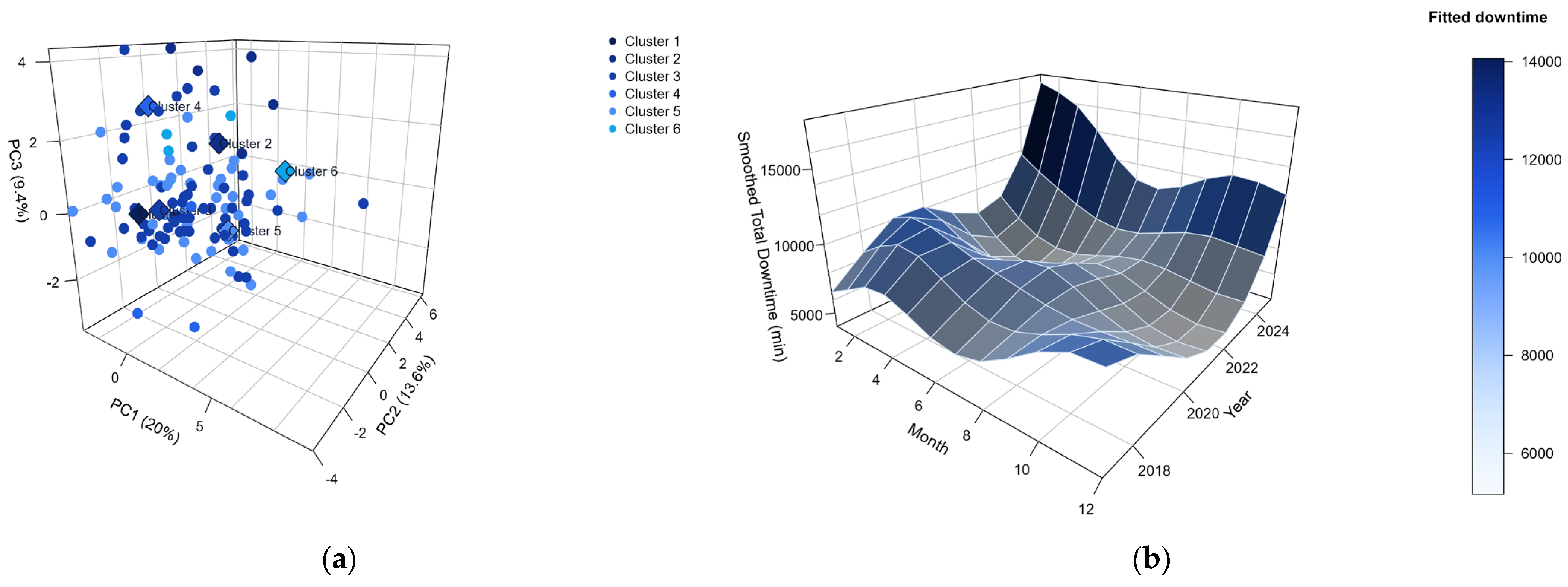
In this equation, $x_{\tau j}$ is the original value of feature $j$ in month $\tau$, ${\bar{x}}_j$ and $s_j$ are its mean and standard deviation, $W_{k }$ is the total within-cluster sum of squares, $C_r$ is cluster $r$, and ${\mu }_{r }$ is the corresponding centroid. The silhouette value $s\left(i\right)$ combines within-cluster cohesion $a\left(i\right)$ and nearest-cluster separation $b\left(i\right)$. Principal component projection, heatmaps of standardised cluster centres, and smoothed three-dimensional surfaces estimated using a Generalised Additive Model (GAM) framework were used to support the interpretation of cluster separation, discriminative feature structure, and non-linear temporal patterns.

A limitation of this study is that the analysis is based on secondary operational records that were not generated as an experimental research dataset. Therefore, the results identify statistical associations, frequency–severity disproportions, forecasting patterns, and exploratory monthly operating regimes, but they should not be interpreted as causal evidence. Monthly aggregation improves modelling stability but may obscure short-term episodes at daily or shift level. The retained clustering solution should also be understood as an interpretable typology rather than as a deterministic classification. In addition, consistent monthly covariates such as production output, operating load, weather conditions, maintenance-shift structure, spare-part availability, equipment age, detailed equipment capacity, and complete intervention history were not available. These missing covariates may represent confounding factors. Despite these limitations, the framework provides a reproducible basis for assessing recorded operational burden, forecasting downtime, and supporting maintenance-oriented decision-making.

4. Results

4.1. Dominant Fault Types by Frequency and Downtime Burden

The analysis of dominant fault types shows a pronounced concentration of operational risk within a small number of fault categories. As shown in

Table 4. Dominant fault types by frequency and downtime burden. Source: own processing in RStudio, R version 4.5.2.

Fault Type	Number of Failures	Share of Failures (%)	Total Downtime (min)	Share of Downtime (%)	Mean Downtime (min)	Median Downtime (min)	90th Percentile Downtime (min)
Collapse	2485	37.6230	378,298	38.6851	152.2326	201.0000	262.0000
Misalignment	1143	17.3051	105,834	10.8227	92.5932	20.0000	258.8000
Belt Slip	826	12.5057	167,063	17.0840	202.2554	254.0000	267.0000
Off-Track Belt	305	4.6177	65,553	6.7035	214.9279	218.0000	265.0000
Tear	260	3.9364	56,540	5.7818	217.4615	218.0000	260.0000
Travel Mechanism	240	3.6336	13,917	1.4232	57.9875	55.0000	55.5000
Motor Failure	122	1.8471	27,618	2.8242	226.3770	217.0000	260.0000
Transfer Chute	122	1.8471	31,026	3.1727	254.3115	258.0000	266.0000
Run-Up	119	1.8017	7569	0.7740	63.6050	55.0000	109.0000
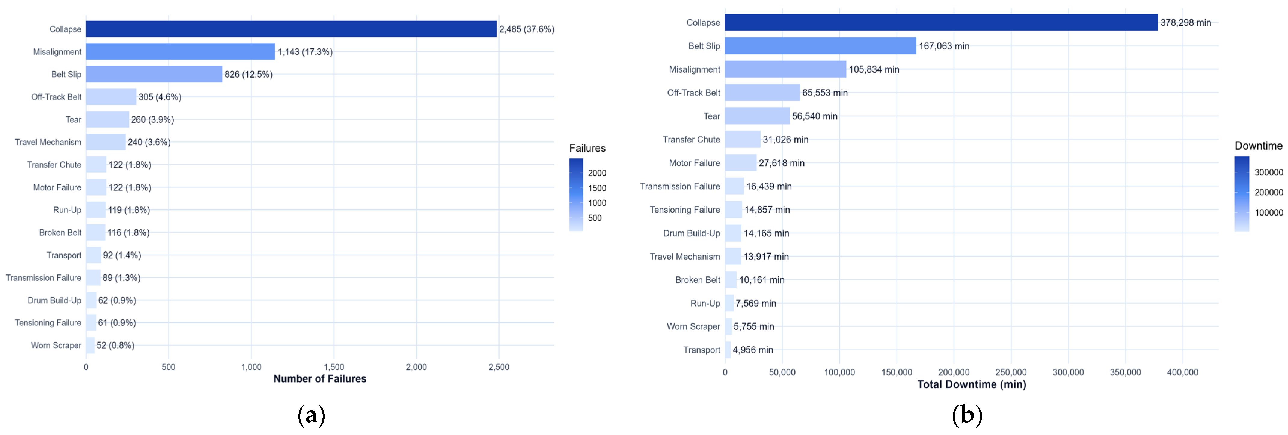
Broken Belt	116	1.7562	10,161	1.0391	87.5948	77.0000	253.0000

, Collapse is the most significant category, accounting for 37.62% of all recorded failures and 38.69% of total downtime. This fault type is therefore the main source of system instability, combining high occurrence with a substantial downtime burden. A particularly important finding is the divergence between frequency-based and downtime-based rankings for Misalignment and Belt Slip. Although Misalignment is the second most frequent fault type, accounting for 17.31% of all failures, it contributes only 10.82% of total downtime. Conversely, Belt Slip occurs less frequently but generates 17.08% of total downtime, indicating higher severity per event.

From a maintenance-management perspective, these results demonstrate the need to distinguish between high-frequency faults and high-severity faults. Categories such as Off-Track Belt, Tear, Motor Failure, and Transfer Chute do not dominate in terms of occurrence frequency, but their mean and median downtime values indicate considerable operational severity. The results therefore support a prioritisation strategy based not only on the number of failures but also on downtime contribution and tail-risk behaviour captured by the 90th percentile of downtime.

The graphical representation of the dominant fault types confirms that the analysed system exhibits a strong concentration of both failure occurrence and downtime burden within a limited number of categories. As shown in Figure 1, the ranking of fault types by occurrence frequency does not fully align with the ranking by total downtime. This discrepancy indicates that failure frequency alone is insufficient to identify the most operationally critical fault categories, and that downtime severity must also be considered. While panel (a) presents the most frequent fault types by number of occurrences, panel (b) illustrates their downtime impact expressed as total downtime.

4.2. Annual and Monthly Dynamics of Failures and Downtime

The annual dynamics of failures and downtime indicate an uneven development of operational reliability over the analysed period. As reported in

Table 5. Annual dynamics of failure occurrence and downtime over 2017–2025. Source: own processing in RStudio, R version 4.5.2.

Year	Number of Failures	Total Downtime (min)	Mean Downtime (min)	Median Downtime (min)	Failure YoY Change (%)	Downtime YoY Change (%)
2017	634	94,943	149.7524	201.0000	–	–
2018	783	130,002	166.0307	211.0000	23.5016	36.9264
2019	720	100,275	139.2708	80.0000	−8.0460	−22.8666
2020	810	126,475	156.1420	207.0000	12.5000	26.1281
2021	673	83,316	123.7979	55.0000	−16.9136	−34.1245
2022	538	76,073	141.3996	203.0000	−20.0594	−8.6934
2023	544	73,160	134.4853	101.0000	1.1152	−3.8292
2024	723	120,758	167.0235	214.0000	32.9044	65.0601
2025	1180	172,888	146.5153	109.0000	63.2089	43.1690

, neither the number of failures nor total downtime follows a simple linear trend. Instead, the pattern is characterised by alternating periods of increased operational burden and partial stabilisation. Higher values were observed in 2018 and 2020, followed by a decline between 2021 and 2023, when total downtime decreased from 83,316 min in 2021 to 73,160 min in 2023. This interval may be interpreted as a phase with a lower aggregated failure burden, although the available results do not allow this decline to be attributed unambiguously to technical, organisational, operational, or external factors.

The most pronounced shift occurred in 2024 and 2025. In 2024, the number of failures increased by 32.90% year-on-year, while total downtime rose by 65.06%. In 2025, the number of failures increased by a further 63.21%, and total downtime increased by 43.17%. Thus, 2025 represents the maximum for the entire observation period in both failure frequency and total downtime. Importantly, however, the mean downtime per failure in 2025 was not the highest value observed across the period. This suggests that the deterioration in 2025 was driven mainly by an increase in failure frequency rather than exclusively by longer individual downtime events.

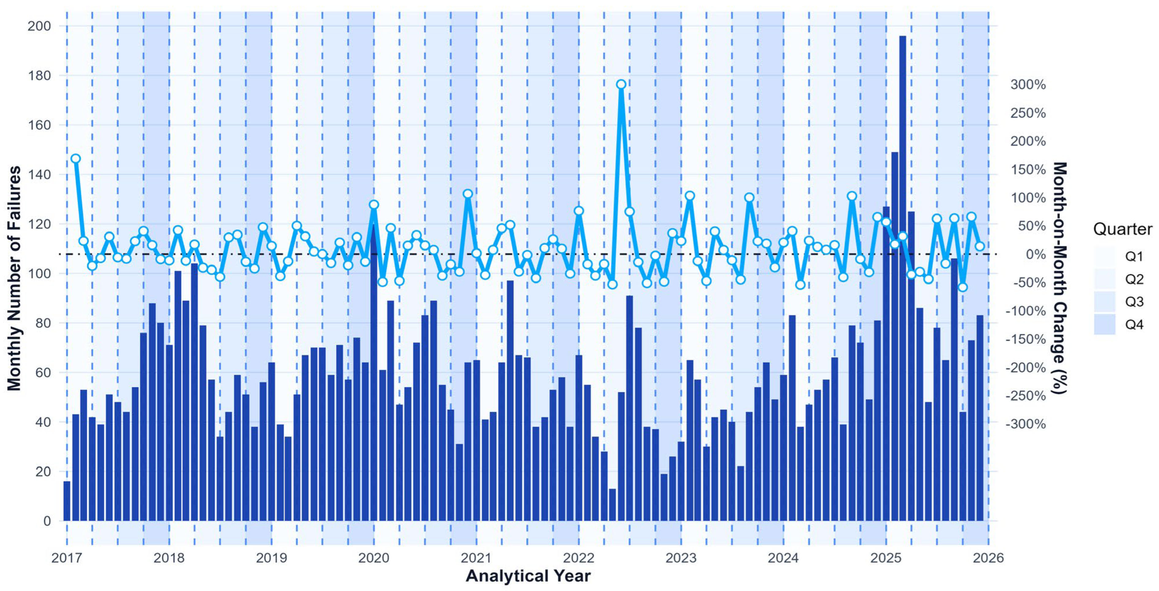
The monthly visualisation in Figure 2 complements the annual aggregates by providing a higher-resolution temporal view of failure dynamics. The bars represent monthly failure counts, whereas the line represents the month-on-month percentage change. The figure shows that failure occurrences were not evenly distributed over time but were characterised by repeated short-term fluctuations. These fluctuations are analytically important because annual aggregation may conceal intra-annual volatility and short periods of accumulated failure events.

Figure 2 also confirms that the final part of the observation period, particularly 2025, was characterised by a higher concentration of monthly failure events. This supports the interpretation in Table 5, which indicates that the increase in the overall operational burden in 2025 was primarily driven by frequency. Nevertheless, pronounced month-on-month percentage changes should be interpreted with caution, as relative indicators may be sensitive to a low base in the preceding month. Therefore, the figure should be understood mainly as evidence of temporal instability and as a basis for subsequent modelling of trends, seasonality, or forecasting, rather than as standalone evidence of statistically confirmed seasonality.

4.3. Forecast Modelling of Failure Counts and Total Downtime

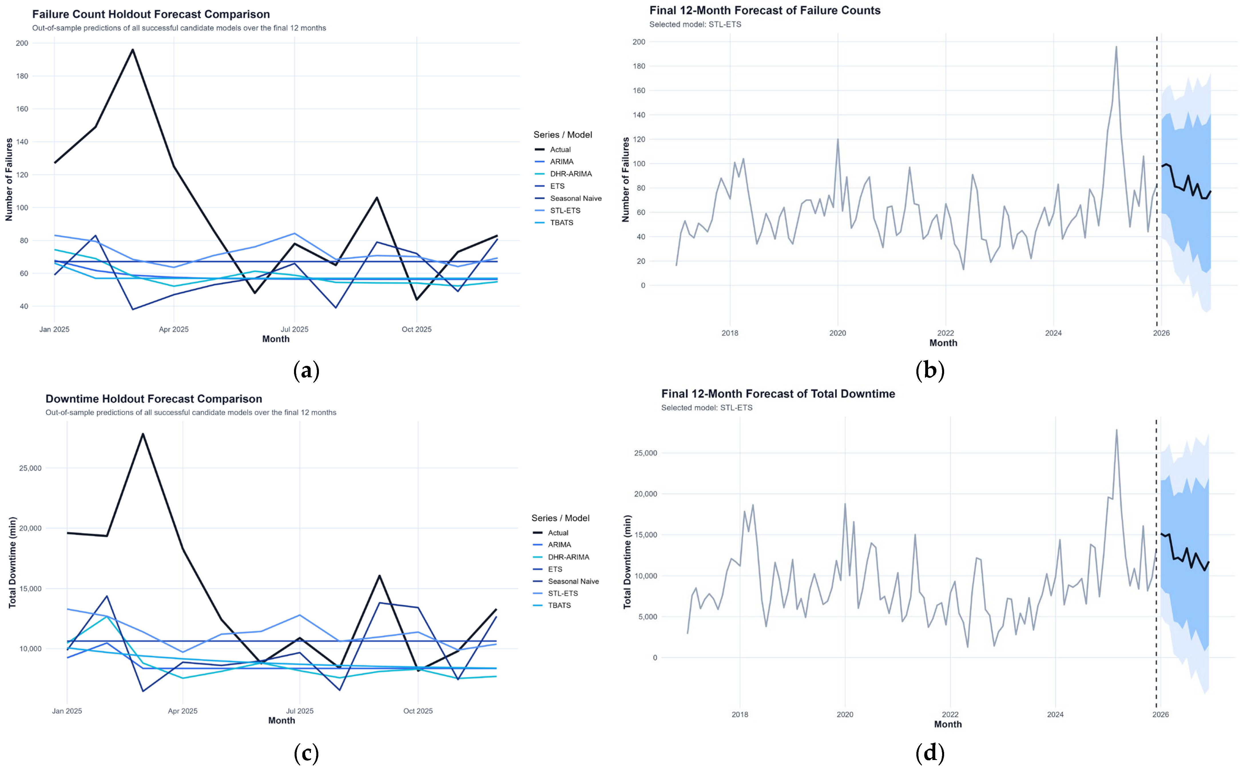
To identify the most appropriate forecasting approach for monthly failure counts and total downtime, the candidate time-series models were compared using the time-ordered holdout validation described in the methodology. As shown in

Table 6. Holdout accuracy of candidate models for failure count. Source: own processing in RStudio, R version 4.5.2.

Metric	STL-ETS	ETS	DHR-ARIMA	ARIMA	TBATS	Seasonal Naive
ME	−25.9439	−31.2087	−39.9939	−40.1797	−40.6101	−38.0833
RMSE	50.0509	52.7766	57.0049	57.4040	58.5058	60.6293
MAE	36.6174	38.6043	43.8807	43.6790	44.2611	44.2500
MAPE (%)	33.8692	34.1298	38.3807	37.6250	37.9915	39.8127
sMAPE (%)	38.2076	40.6505	48.9118	48.1816	48.9111	50.5246

and

Table 7. Holdout accuracy of candidate models for total downtime. Source: own processing in RStudio, R version 4.5.2.

Metric	STL-ETS	ETS	TBATS	Seasonal Naive	DHR-ARIMA	ARIMA
ME	−3091.3723	−3771.2388	−5471.6155	−4344.1667	−5755.3398	−5795.8634
RMSE	6386.9282	6865.9176	7675.8330	7761.4209	7808.7159	8023.7224
MAE	4774.0359	5005.9685	5566.1473	5253.5000	5783.5325	5827.9456
MAPE (%)	29.2105	29.3056	30.6148	31.3982	32.8567	32.1693
sMAPE (%)	33.0935	34.8111	39.9532	38.3664	43.1181	42.5652

, Seasonal and Trend decomposition using Loess combined with exponential smoothing (STL-ETS) achieved the best holdout performance for both analysed series across the main error measures. All models yielded negative mean errors (ME), indicating systematic underprediction of the validation observations; however, this bias was smallest for STL-ETS. This underprediction is likely related to the abrupt increase in operational burden observed toward the end of the analytical period, which was difficult for models calibrated on earlier, lower-intensity observations to fully reproduce. The results, therefore, indicate not only forecast bias but also a limitation of purely univariate forecasting when sudden regime shifts or operational intensification occur. For this reason, the forecasts should be interpreted as probabilistic decision-support estimates rather than deterministic predictions of future failures or downtime.

The diagnostic characteristics of the selected models, reported in

Table 8. Diagnostics of selected models and aggregate 12-month forecast summary. Source: own processing in RStudio, R version 4.5.2.

Indicator	Failure Count	Total Downtime
Selected model	STL-ETS	STL-ETS
Seasonal strength	0.0622	0.1074
Trend strength	0.3411	0.4356
Peak month	2	3
Trough month	8	8
Lag-12 ACF	−0.0678	−0.0177
Ljung–Box p-value	0.00555	0.06808
RMSE	50.0509	6386.9282
MAE	36.6174	4774.0359
sMAPE (%)	38.2076	33.0935
Forecast start	2026-01	2026-01
Forecast end	2026-12	2026-12
Forecast horizon (months)	12	12
Mean monthly forecast	83.5151	12,686.2446
Total 12-month forecast	1002.1816	152,234.9352
Minimum monthly forecast	71.4815	10,670.1325
Maximum monthly forecast	99.4966	15,139.0160
Average 95% interval width	157.4969	25,808.4834

, indicate relatively weak seasonality but a mild to moderate trend component in both series. For failure count, seasonal strength was 0.0622 and trend strength 0.3411, whereas for total downtime, the respective values were 0.1074 and 0.4356. Peak months were identified as February for failure count and March for total downtime, while the lowest values were concentrated in August for both series. From the perspective of residual diagnostics, the Ljung–Box p-value for the total downtime model was 0.06808, which does not indicate a serious violation of residual independence at the conventional significance level. By contrast, the model for failure count yielded p = 0.00555, indicating that some residual autocorrelation remained in the count series. This result suggests that the selected STL-ETS model did not fully capture all temporal dependence in monthly failure counts. The forecast for failure occurrence should therefore be interpreted with caution, and future model extensions should consider exogenous operational covariates, such as production intensity, operating load, maintenance interventions, or environmental conditions, where such data are available. ARCH-type or other volatility-sensitive specifications may also be considered if future data show time-varying residual variance.

The aggregate 12-month forecast in Table 8 indicates a mean monthly forecast of 83.5151 failure events and 12,686.2446 min of total downtime, corresponding to annual totals of 1002.1816 failures and 152,234.9352 min of downtime. The month-by-month projections in

Table 9. Month-by-month final forecasts with 95% prediction intervals for 2026. Source: own processing in RStudio, R version 4.5.2.

Month	Failure Count Mean	Failure Count Lower 95%	Failure Count Upper 95%	Total Downtime Mean	Total Downtime Lower 95%	Total Downtime Upper 95%
2026-01	97.5040	38.8575	156.1505	15,139.0160	5197.6335	25,080.3986
2026-02	99.4966	36.7340	162.2591	14,811.3813	4275.7145	25,347.0481
2026-03	97.7826	31.0959	164.4693	15,047.8357	3940.3708	26,155.3006
2026-04	81.1766	10.7247	151.6284	12,051.7217	391.4862	23,711.9573
2026-05	80.1691	6.0858	154.2524	12,214.8509	18.1392	24,411.5626
2026-06	77.9820	0.3813	155.5828	11,789.7060	0.0000	24,508.8038
2026-07	90.1066	9.0868	171.1264	13,345.2129	116.0108	26,574.4150
2026-08	73.8944	0.0000	158.2477	11,002.2766	0.0000	24,730.8066
2026-09	83.2593	0.0000	170.8712	12,747.7367	0.0000	26,966.0872
2026-10	71.6364	0.0000	162.4410	11,651.1536	0.0000	26,350.8995
2026-11	71.4815	0.0000	165.4204	10,670.1325	0.0000	25,843.7802
2026-12	77.6925	0.0000	174.7135	11,763.9112	0.0000	27,404.7761

Note: Negative lower bounds generated by the parametric prediction interval procedure were truncated to zero because failure counts and downtime cannot take negative values in operational interpretation. The truncation affects only the practical presentation of the lower interval bounds and not the point forecasts or upper prediction limits. This issue is acknowledged as a limitation of the current univariate forecasting approach.

indicate higher expected values mainly at the beginning of 2026, followed by a moderate decline in later months. However, the relatively wide 95% prediction intervals, especially for downtime, indicate substantial forecast uncertainty. Because failure counts and downtime are non-negative operational quantities, negative lower prediction bounds produced by the parametric interval procedure were truncated to zero in Table 9. This improves practical interpretability but also highlights a limitation of the current univariate forecasting approach; future work should consider transformed-scale forecasting, bootstrap-based prediction intervals, quantile regression, or count-specific non-negative forecasting models.

Figure 3 summarises the holdout comparison of candidate models and the final 12-month forecasts of the selected STL-ETS model. The validation panels confirm that STL-ETS provided the closest agreement with the observed values for both failure counts and total downtime, while the forecast panels indicate partial stabilisation in 2026 at a still elevated level. The prediction intervals also show that uncertainty remains more pronounced for total downtime than for failure counts.

4.4. Machine-Level Differences in Downtime Severity and Testing of Calendar-Month Effects

The inferential analysis confirmed that downtime severity differs significantly across machine categories, whereas calendar month did not emerge as a systematic determinant of either failure occurrence or total downtime. As shown in

Table 10. Downtime severity across machine categories. Source: own processing in RStudio, R version 4.5.2.

Machine Category	n	Mean Downtime (min)	Median Downtime (min)	SD Downtime (min)	IQR Downtime (min)
P―Conveyor Belt	3395	239.7143	253.0000	27.1539	46.0000
R―Excavator	2710	49.1299	55.0000	27.5610	35.0000
Z―Stacker	500	61.8360	78.5000	39.3566	82.0000

, conveyor belts exhibit by far the highest downtime burden, with both the mean downtime per event (239.7143 min) and the median downtime (253.0000 min) highest. This indicates that this equipment class makes the dominant contribution to overall operational inefficiency. Excavators, by contrast, show the lowest downtime severity (mean 49.1299 min; median 55.0000 min), while stackers occupy an intermediate position in terms of central tendency but display the highest within-group variability (SD = 39.3566; IQR = 82.0000). This pattern suggests that downtime events associated with stackers are more heterogeneous and may encompass a broader range of operational failure scenarios.

The robustness of these differences is further confirmed by the formal inferential tests reported in

Table 11. Inferential tests of machine-level differences and calendar-month effects. Source: own processing in RStudio, R version 4.5.2.

Testing Domain	Method	df1	df2	Test Statistic	p-Value	Effect Size
Machine-level differences in downtime	One-way ANOVA on log1p (downtime_min)	2	6602	F = 6795.1	<0.00001	Eta squared = 0.67304
Machine-level differences in downtime	Welch ANOVA on log1p (downtime_min)	2	1144	F = 10313.7	<0.00001	–
Machine-level differences in downtime	Kruskal–Wallis test on downtime_min	2	–	Chi-square = 4985.0	<0.00001	Epsilon squared = 0.75477
Machine-level differences in downtime	Brown-Forsythe/Levene (median-centred)	2	6602	F = 925.04	<0.00001	–
Calendar-month effect on failure count	ANOVA	11	96	F = 0.434	0.93723	Eta squared = 0.04735
Calendar-month effect on failure count	Kruskal–Wallis test	11	–	Chi-square = 3.674	0.97849	Epsilon squared = 0.00000
Calendar-month effect on total downtime	ANOVA	11	96	F = 0.437	0.93543	Eta squared = 0.04772
Calendar-month effect on total downtime	Kruskal–Wallis test	11	–	Chi-square = 5.374	0.91172	Epsilon squared = 0.00000

. A one-way ANOVA performed on the log-transformed variable log1p(downtime_min) identified highly significant differences across machine categories $\left(F = 6795.05496; p < 0.00001\right)$, with a very large effect size $({\eta }^2 = 0.67304)$, indicating that machine category explains a substantial proportion of the variability in downtime severity. The same conclusion is supported by Welch’s ANOVA, which accounts for unequal variances, as well as by the non-parametric Kruskal–Wallis test $\left({\chi }^2 = 4984.99264; p < 0.00001; {\epsilon }^2 = 0.75477\right)$. In addition, the Brown–Forsythe/Levene test confirmed variance heterogeneity across groups $\left(F = 925.03924; p < 0.00001\right)$, thereby supporting the decision to rely on both parametric and non-parametric validation strategies.

Subsequent post hoc analyses showed that all pairwise comparisons between machine categories were statistically significant. Tukey’s HSD test on the log-transformed values confirmed significant contrasts for all three category pairs $(p_{\mathrm{adj}} < 0.00001)$, and the Dunn–Holm post hoc procedure on the original scale reached the same conclusion $(p_{\mathrm{adj}} < 0.00001)$. In substantive terms, this means that the differences among conveyor belts, excavators, and stackers are not only statistically detectable but also operationally meaningful and consistent across alternative analytical frameworks.

By contrast, calendar month did not prove to be a significant factor for either failure count or total downtime. For failure count, both ANOVA $\left(F = 0.43374; p = 0.93723\right)$ and the Kruskal–Wallis test $\left({\chi }^2 = 3.67435; p = 0.97849\right)$ were clearly non-significant. The same pattern held for total downtime, where both ANOVA $\left(F = 0.43730; p = 0.93543\right)$ and the Kruskal–Wallis test $\left({\chi }^2 = 5.37385; p = 0.91172\right)$ failed to identify significant month-of-year differences. Effect sizes were negligible in all cases. These findings indicate that the monthly fluctuations observed in the time-series analysis should not be interpreted as stable calendar-based seasonality, but rather as irregular operational variability, episodic failure clustering, or the influence of external operational conditions.

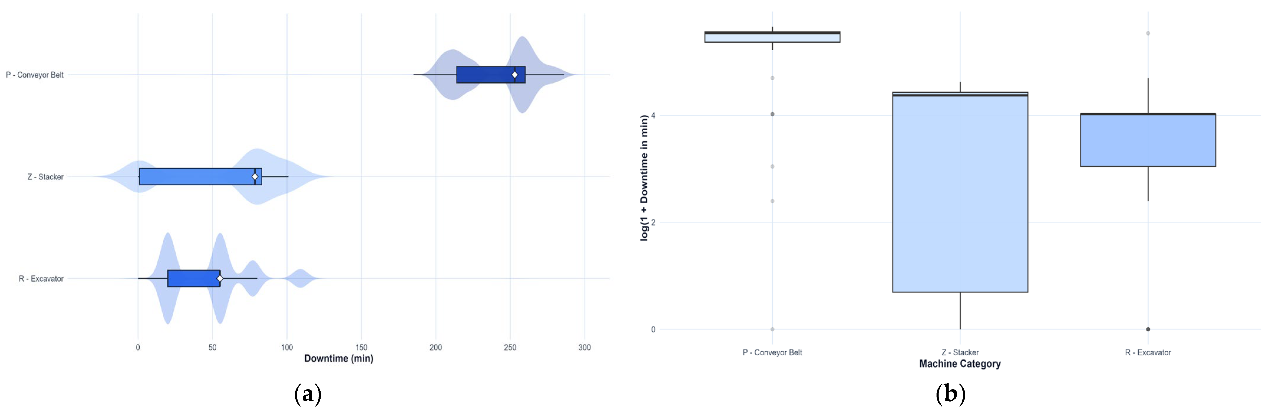
The graphical evidence in Figure 4 visually reinforces the conclusion that downtime severity differs markedly across machine categories. Figure 4a presents the downtime distributions on the original scale and shows a clear shift in conveyor belts toward substantially higher values than in the other equipment classes. Figure 4b then displays the dispersion of the log-transformed values used in the inferential analysis. Even after transformation, clear between-group separation remains evident, supporting both the robustness of the observed differences and the suitability of the chosen analytical procedure.

4.5. Cluster Structure of Monthly Operating States and Profiling of the Retained Solution

To identify typical monthly operating regimes, cluster analysis was applied to the monthly aggregated dataset, and candidate solutions with k = 4 to k = 8 clusters were evaluated using the average silhouette width, total within-cluster sum of squares, between-cluster sum of squares, and substantive interpretability. The retained six-cluster solution was selected because it provided practically interpretable operating-regime profiles that were consistent with the subsequent visualisations and a maintenance-oriented interpretation. However, the relatively low silhouette value indicates that the monthly observations do not form sharply separated natural classes. Therefore, the cluster solution is interpreted as an exploratory typology of monthly operating regimes rather than as a deterministic classification model.

The comparison of alternative cluster solutions indicated that increasing the number of clusters did not produce a clearly more maintenance-relevant segmentation. Additional clusters are mainly subdivided into already interpretable regimes without generating a substantially distinct operational profile. For this reason, the six-cluster solution was retained as a parsimonious and practically interpretable representation of the main monthly operating regimes.

As shown in

Table 12. Profile of the retained six-cluster solution of monthly operating states. Source: own processing in RStudio, R version 4.5.2.

Indicator	Cluster 1	Cluster 2	Cluster 3	Cluster 4	Cluster 5	Cluster 6
Number of months	2	16	45	8	30	7
Mean failures	47.5000	82.6250	65.9333	40.1250	56.9333	27.4286
Median failures	47.5000	69.5000	64.0000	40.5000	57.0000	30.0000
Mean total downtime (min)	7844.5000	12,116.813	10,879.200	6352.2500	6932.1000	2855.2857
Median total downtime (min)	7844.5000	9738.5000	10,255.000	6615.5000	6975.0000	3136.0000
Mean downtime per event (min)	166.0966	149.7355	165.6011	161.4784	121.5172	102.3425
Median event downtime (min)	204.7500	149.3750	213.9778	206.5625	69.0500	64.8571
90th percentile downtime (min)	270.5000	269.9750	263.3133	235.6750	253.5400	199.6429
Mean active fault types	10.5000	14.0625	12.0000	8.1250	11.6333	8.4286
Mean active devices	2.5000	2.9375	2.9333	2.8750	2.9333	2.8571

, the retained solution reveals heterogeneous monthly operating states. Cluster 3 was the most frequent regime and represents a baseline state with intermediate failure occurrence and downtime burden. Cluster 5 describes recurrent but less severe operating conditions, while Cluster 2 represents a high-burden regime with elevated failure counts and total downtime. Cluster 4 captures more favourable months with lower failure counts and downtime, whereas Cluster 6 represents the mildest regime. Cluster 1, although represented by only two months, reflects an atypical episodic deterioration state with a marked increase in failures and downtime.

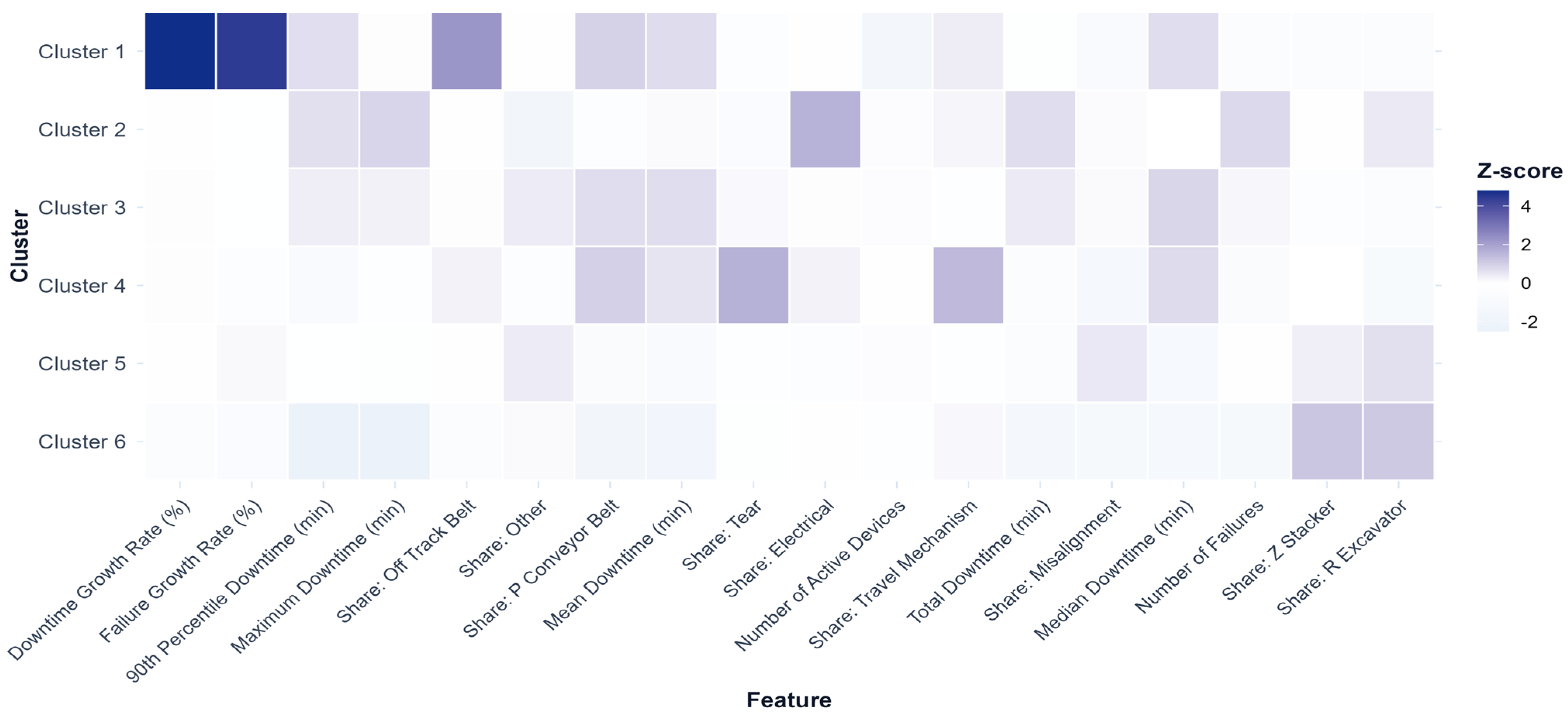
The discriminative feature analysis further indicates that the clusters differ not only in intensity but also in equipment and fault-type composition. Cluster 1 is associated with strong growth dynamics and Off-Track Belt events; Cluster 2 with electrical and planned events and higher maximum downtime; Cluster 3 with conveyor-belt-related downtime severity; Cluster 4 with Tear, Travel Mechanism, and Collapse failures; Cluster 5 with excavator-related and Misalignment events; and Cluster 6 with comparatively low upper-tail downtime risk. Overall, the retained solution should be interpreted as an exploratory regime typology that helps distinguish baseline months, elevated-burden states, mechanically specific profiles, and atypical deterioration episodes.

The graphical interpretation in Figure 5 complements the tabular cluster profiles by simultaneously showing the separation of operating regimes in a reduced multivariate feature space and the smooth month-by-year structure of downtime burden. Figure 5a shows the spatial arrangement of monthly observations in the space of the first three principal components under the retained k = 6 solution. Although the clusters are not completely disjoint, the visualisation reveals recognisable local groupings, supporting the substantive plausibility of the selected segmentation structure. Figure 5b then presents the smoothed three-dimensional surface of total monthly downtime estimated using a GAM framework. The surface indicates that downtime burden follows a non-linear temporal pattern, with higher levels concentrated in selected periods rather than forming a stable, uniform trend. Taken together, the two panels support the conclusion that monthly operating states are structurally differentiated and jointly associated with changes in operational burden over time.

Figure 6 further supports the interpretation of the retained six-cluster solution by showing the standardised cluster-centre heatmap. The heatmap indicates that the clusters are differentiated not only by failure intensity and downtime burden, but also by equipment involvement, fault-type composition, and temporal growth dynamics. Cluster 1 is the most distinctive profile, with high positive z-scores for downtime growth, failure growth, and Off-Track Belt share, supporting its interpretation as an episodic deterioration regime. The remaining clusters show more specific operational profiles: Cluster 2 is associated with electrical and planned events; Cluster 3 with conveyor-belt-related downtime severity; Cluster 4 with Tear, Travel Mechanism, and Collapse failures; Cluster 5 with excavator-related and Misalignment events; and Cluster 6 with comparatively low upper-tail downtime risk. Overall, Figure 6 confirms that the retained clusters represent an exploratory typology of operating regimes rather than arbitrary partitions of monthly observations.

Heatmap of standardised cluster centres for the retained k = 6 solution, showing the relative prominence of the most discriminative variables across monthly operating regimes. The figure highlights differences among clusters in growth dynamics, downtime severity, equipment structure, and fault-type composition, thereby complementing the spatial and temporal interpretation presented in Figure 5.

It should also be noted that some clustering variables are not fully independent from a mathematical perspective. In particular, total monthly downtime depends on both the number of failures and the average downtime per event. These variables were retained because they represent different operational interpretations: frequency intensity, cumulative downtime burden, and event-level severity. However, their partial dependence may increase the weight of the downtime-intensity dimension during clustering. For this reason, the cluster solution should be interpreted as an exploratory regime typology rather than as a fully independent latent structure. Future work may test alternative feature sets, dimensionality-reduction-based clustering, or model-based clustering to assess the robustness of the identified regimes.

5. Discussion

The results of this study broadly align with the current literature on predictive maintenance and reliability modelling, while also extending it in an important direction. Previous studies have shown that industrial failure processes should not be understood solely as isolated technical events, but as temporally structured operational phenomena that require data-driven monitoring, time-series modelling, and maintenance-oriented interpretation [1,2,3,4,5,6,7,8,9,10]. This was confirmed in the present analysis, in which both failure counts and downtime varied unevenly over time and were characterised by episodic increases rather than a simple linear trajectory. The sharp rise in failure frequency and total downtime in 2024–2025 supports the view that operational reliability in material-handling systems is dynamic and may deteriorate rapidly over relatively short periods. This finding aligns with studies emphasising the importance of real-time monitoring, predictive modelling, and early-warning diagnostics in industrial systems [6,7,8,9,10].

A particularly strong confirmation of the literature concerns the critical role of conveyor systems. Prior research has repeatedly identified conveyor systems as technologically important elements whose failures can interrupt material flow and generate secondary operational losses [11,12,13,14,15]. The present results strongly support this argument. Conveyor belts accounted for 51.40% of all failure events but as much as 83.22% of total downtime, indicating that their operational impact was substantially higher than their share of failures alone would suggest. This finding confirms that conveyor systems should be treated not only as frequently failing components but also as dominant contributors to system-level downtime severity. In this respect, the study strengthens the conclusions of the conveyor-focused predictive maintenance literature by providing empirical evidence of a clear frequency–severity imbalance.

The results also support the argument that failure frequency alone is insufficient for maintenance prioritisation. Previous studies have shown that failure type, component degradation, and operational context can substantially influence downtime duration and system consequences [31,32,33,34,35,36,37,38,39,40,65]. This was clearly observed in the comparison of dominant fault types. For example, Misalignment was the second most frequent fault type, but its share of total downtime was lower than its share of failures. Conversely, Belt Slip occurred less frequently than Misalignment but caused greater downtime. Similarly, Transfer Chute, Motor Failure, Tear, and Off-Track Belt did not dominate by frequency, but their mean and median downtime values indicated substantial severity. These findings confirm the need to combine frequency-based and severity-based indicators when identifying maintenance priorities. From a practical perspective, the results show that maintenance decisions based only on the number of failures may systematically underestimate less frequent but more time-critical fault mechanisms.

The inferential results further support earlier studies showing that equipment categories differ in reliability behaviour and operational consequences [19,27,31,32]. The highly significant machine-level differences in downtime severity, confirmed by ANOVA, Welch ANOVA, Kruskal–Wallis tests, and post hoc comparisons, demonstrate that equipment category is a major determinant of downtime burden. The very large effect sizes indicate that these differences are not only statistically significant but also operationally meaningful. This finding aligns with the literature emphasising component-specific diagnostics and differentiated maintenance strategies [15,19,20]. At the same time, the results go beyond many previous studies by showing that device-level differences remain robust across both parametric and non-parametric testing frameworks.

In contrast, the analysis did not confirm a stable calendar-month effect on either failure counts or total downtime. This is an important finding because time-series visualisations showed visible monthly fluctuations, but formal tests indicated that these fluctuations were not systematically tied to calendar months. This result suggests that the observed temporal variability should be interpreted as irregular operational instability, episodic clustering, or process-specific variation rather than as regular seasonality. It also complements the forecasting diagnostics, where seasonal strength was low for both failure counts and downtime. Therefore, unlike studies that emphasise recurring temporal patterns or seasonal forecasting structures [3,16,24], the present results indicate that, in this dataset, operational variability is more irregular than calendar-driven variability.

The forecasting analysis partially confirmed the relevance of time-series models highlighted in the literature [3,16,21,22,23,24,25]. Among the candidate models, STL-ETS achieved the best holdout performance for both failure counts and total downtime, indicating that decomposition-based exponential smoothing is suitable for capturing the dominant temporal structure of the analysed data. However, the results also show limitations. All models tended to underpredict actual values, and the failure-count model exhibited some residual dependence, as indicated by the Ljung–Box test. This means that although forecasting models provide useful operational expectations, they should not be interpreted as fully capturing all failure-generating mechanisms. This finding is consistent with the literature highlighting the complexity of industrial failure processes and the limits of purely statistical forecasting when contextual operational variables are incomplete [18,20,45].

The cluster analysis provides an exploratory extension of the literature by suggesting that monthly operating states can be interpreted as several recurring regimes rather than as a fully homogeneous continuous process. Previous studies have argued that failure behaviour is multivariate and shaped by the joint interaction of frequency, severity, equipment structure, fault type, and temporal dynamics [48,49,50,51,52,53,54,55,56,57,58,59,60,61]. The retained six-cluster solution provides exploratory support for this view. Although the silhouette values were relatively low, indicating overlapping rather than sharply separated groups, the clusters were substantively interpretable. They distinguished baseline months, high-burden regimes, mild regimes, mechanically specific regimes, and episodic deterioration states. This confirms that clustering is useful not as a rigid classification tool, but as an exploratory framework for translating complex maintenance data into interpretable operating regimes.

Overall, the study confirms several key directions in the literature: the importance of predictive maintenance, the critical role of conveyor systems, the insufficiency of failure frequency alone, the relevance of downtime-oriented metrics, and the value of multivariate regime identification. At the same time, it provides a more integrated contribution by combining frequency–severity analysis, inferential testing, forecasting validation, and cluster-based interpretation within one analytical framework. The main added value lies in showing that operational risk is not evenly distributed across devices, fault types, or months. Instead, it is concentrated in specific equipment categories, selected fault mechanisms, and identifiable operating regimes. The main added value lies in showing that recorded operational burden is not evenly distributed across devices, fault types, or monthly operating states. Instead, it is concentrated in specific equipment categories, selected fault mechanisms, and identifiable exploratory regimes. These findings may support maintenance prioritisation and decision-making by highlighting where downtime burden is most pronounced. However, because the study is based on observational secondary records, the results should be interpreted as evidence of statistical and operational associations rather than as proof of causal mechanisms.

6. Conclusions

This study developed an integrated analytical framework for examining operational failures and downtime in a continuous material-handling and technological transport process. Regarding RQ1, the results showed that downtime burden was not proportional to failure frequency. Conveyor belts accounted for a substantially higher share of total downtime than would be expected from their share of failure events, and several less frequent fault mechanisms, including Belt Slip, Off-Track Belt, Tear, Motor Failure, and Transfer Chute, resulted in considerable downtime severity. This confirms that maintenance prioritisation based solely on failure counts may underestimate the operational criticality of fault mechanisms.

Regarding RQ2, the inferential results confirmed statistically significant and operationally meaningful differences in downtime severity across machine categories. The robustness of these differences was supported by ANOVA, Welch ANOVA, Kruskal–Wallis tests, and post hoc procedures. In contrast, calendar month was not identified as a significant determinant of monthly failure counts or total downtime, suggesting that the observed temporal fluctuations reflect irregular operational variability rather than stable calendar-based seasonality.

In response to RQ3, the forecasting analysis showed that STL-ETS provided the best holdout performance for both monthly failure counts and total downtime. The 2026 projections indicate partial stabilisation relative to the extreme values observed at the end of the analysed period, although the relatively wide prediction intervals, especially for downtime, reflect substantial uncertainty. Forecasting should therefore be interpreted as a probabilistic decision-support tool for maintenance planning rather than as a deterministic prediction of future failures.

Finally, with respect to RQ4, the cluster analysis suggested that monthly operating states can be grouped into interpretable exploratory regimes. The retained six-cluster solution provided an exploratory differentiation of baseline months, elevated-burden regimes, mild operating periods, mechanically specific profiles, and episodic deterioration states. The standardised feature heatmap further confirmed that these regimes differ not only in failure intensity and downtime burden, but also in equipment involvement, fault-type composition, and temporal growth dynamics.

The main contribution of the study lies in integrating frequency–severity analysis, inferential validation, forecasting, and clustering into one reproducible exploratory framework. This approach provides a broader understanding of how recorded operational failures are associated with downtime burden and may support maintenance-oriented prioritisation based on differentiated risk profiles rather than aggregate failure counts alone.

Several limitations should be acknowledged. The analysis is based on anonymised secondary operational records that were not originally generated for experimental research; therefore, the results identify statistical associations and operational patterns rather than causal mechanisms. Monthly aggregation improves modelling stability but may obscure short-term events at daily, shift, or operational-cycle resolution. The cluster solution is exploratory and should be understood as an interpretable typology rather than a deterministic classification. In addition, contextual variables such as production volume, operating load, weather conditions, maintenance interventions, maintenance-shift structure, spare-part availability, equipment age, and detailed equipment capacity were not consistently available. These missing covariates may act as confounding factors and should be considered in future extensions of the framework.

Future research should extend this framework using higher-frequency data, additional operational covariates, and methods capable of modelling transitions between operating regimes. Machine learning, survival analysis, and early-warning models could help identify precursors of high-burden states. Validation across other material-handling systems, energy-intensive operations, and continuous-process industries would further strengthen the generalisability of the proposed frequency–severity and regime-based approach. Transferability to sectors such as automotive assembly or pharmaceutical continuous manufacturing would require comparable event-level downtime records, consistent equipment and fault-type coding, and sufficient temporal coverage to support forecasting and regime identification.

References

- Anusha, P.V.S.; Swapna, P.; Reddy, D.V.R.K. Revolutionizing Conveyor Belt Systems: Empowering Predictive Maintenance with IoT, Cloud, and Machine Learning. Int. J. Electr. Electron. Eng. 2024, 11, 224–233. [Google Scholar] [CrossRef]
- Mohan, T.; Roselyn, J.P.; Uthra, R.; Devaraj, D.; Umachandran, K. Intelligent machine learning based total productive maintenance approach for achieving zero downtime in industrial machinery. Comput. Ind. Eng. 2021, 157, 107267. [Google Scholar] [CrossRef]
- Fatima, S.S.W.; Rahimi, A. A Review of Time-Series Forecasting Algorithms for Industrial Manufacturing Systems. Machines 2024, 12, 380. [Google Scholar] [CrossRef]
- Čabaníková, L.; Ambriško, Ľ. Failure analysis of conveyors using the RBI method. Transp. Logist. Int. J. 2025, 25, 10–18. [Google Scholar] [CrossRef]
- Dindarloo, S.R. Reliability Forecasting of a Load-Haul-Dump Machine: A Comparative Study of ARIMA and Neural Networks. Qual. Reliab. Eng. Int. 2016, 32, 1545–1552. [Google Scholar] [CrossRef]
- Wu, M.; Goh, K.W.; Chaw, K.H.; Koh, Y.S.; Dares, M.; Yeong, C.F.; Su, E.L.M.; Holderbaum, W.; Zhang, Y. An intelligent predictive maintenance system based on random forest for addressing industrial conveyor belt challenges. Front. Mech. Eng. 2024, 10, 1383202. [Google Scholar] [CrossRef]
- Mendes, D.; Gaspar, P.D.; Charrua-Santos, F.; Navas, H. Enhanced Real-Time Maintenance Management Model—A Step toward Industry 4.0 through Lean: Conveyor Belt Operation Case Study. Electronics 2023, 12, 3872. [Google Scholar] [CrossRef]
- Pulcini, V.; Modoni, G.E. Machine learning-based digital twin of a conveyor belt for predictive maintenance. Int. J. Adv. Manuf. Technol. 2024, 133, 6095–6110. [Google Scholar] [CrossRef]
- Matos, S.N.; Coletti, O.F.; Zimmer, R.; Filho, F.U.; de Carvalho, R.C.L.; da Silva, V.R.; Franco, J.L.; Pinto, T.V.B.; de Barros, L.G.D.; Ranieri, C.M.; et al. Machine Learning Techniques for Improving Multiclass Anomaly Detection on Conveyor Belts. In Proceedings of the IEEE International Instrumentation and Measurement Technology Conference (I2MTC), Glasgow, UK, 20–23 May 2024; pp. 1–6. [Google Scholar] [CrossRef]
- Ogunmilua, O.O. Failure Rate Prediction of Belt Conveyor Systems using 2-parameter Weibull distribution. Int. J. Res. Appl. Sci. Eng. Technol. 2021, 9, 1035–1039. [Google Scholar] [CrossRef]
- Ahmadi, S.; Moosazadeh, S.; Hajihassani, M.; Moomivand, H.; Rajaei, M. Reliability, availability and maintainability analysis of the conveyor system in mechanized tunneling. Measurement 2019, 145, 756–764. [Google Scholar] [CrossRef]
- García, J.; Rios-Colque, L.; Peña, Á.; Rojas, L. Condition Monitoring and Predictive Maintenance in Industrial Equipment: An NLP-Assisted Review of Signal Processing, Hybrid Models, and Implementation Challenges. Appl. Sci. 2025, 15, 5465. [Google Scholar] [CrossRef]
- Anusha, P.V.S.; Swapna, P.; Reddy, D.V.R.K. Digital transformation technologies for conveyor belts predictive maintenance: A review. Indones. J. Electr. Eng. Comput. Sci. 2024, 36, 639–646. [Google Scholar] [CrossRef]
- Kiangala, K.S.; Wang, Z. An Effective Predictive Maintenance Framework for Conveyor Motors Using Dual Time-Series Imaging and Convolutional Neural Network in an Industry 4.0 Environment. IEEE Access 2020, 8, 121033–121049. [Google Scholar] [CrossRef]
- Al-Kahwati, K.; Saari, E.; Birk, W.; Atta, K. Condition Monitoring of Rollers in Belt Conveyor Systems. In Proceedings of the 5th International Conference on Control and Fault-Tolerant Systems (SysTol), Saint-Raphael, France, 29 September–1 October 2021; pp. 341–347. [Google Scholar] [CrossRef]
- Syed, M.A.B.; Hasan, M.R.; Chowdhury, N.I.; Rahman, M.H.; Ahmed, I. A systematic review of time series algorithms and analytics in predictive maintenance. Decis. Anal. J. 2025, 15, 100573. [Google Scholar] [CrossRef]
- Pal, S.; Koley, A.; Ranjan, P.; Kundu, D. Modeling time to failure using a temporal sequence of events. Qual. Eng. 2025, 37, 493–512. [Google Scholar] [CrossRef]
- Leukel, J.; González, J.; Riekert, M. Adoption of machine learning technology for failure prediction in industrial maintenance: A systematic review. J. Manuf. Syst. 2021, 61, 87–96. [Google Scholar] [CrossRef]
- Liu, X.; He, D.; Lodewijks, G.; Pang, Y.; Mei, J. Integrated decision making for predictive maintenance of belt conveyor systems. Reliab. Eng. Syst. Saf. 2019, 188, 347–351. [Google Scholar] [CrossRef]
- Rzeszowska, A.; Jurdziak, L.; Błażej, R.; Lewandowicz, P. Analysis of Uncertainty in Conveyor Belt Condition Assessment Using Time-Based Indicators. Appl. Sci. 2025, 15, 7939. [Google Scholar] [CrossRef]
- Kazemi, M.M.K.; Nabavi, Z.; Rezakhah, M.; Masoudi, A. Application of XGB-based metaheuristic techniques for prediction time-to-failure of mining machinery. Syst. Soft Comput. 2023, 5, 200061. [Google Scholar] [CrossRef]
- Webb, C.; Sikorska, J.; Khan, R.N.; Hodkiewicz, M. Developing and evaluating predictive conveyor belt wear models. Data-Centric Eng. 2020, 1, e3. [Google Scholar] [CrossRef]
- Shahin, M.; Chen, F.F.; Hosseinzadeh, A.; Zand, N. Using machine learning and deep learning algorithms for downtime minimization in manufacturing systems: An early failure detection diagnostic service. Int. J. Adv. Manuf. Technol. 2023, 128, 3857–3888. [Google Scholar] [CrossRef]
- Baptista, M.; Sankararaman, S.; Medeiros, I.; Nascimento, C.; Prendinger, H.; Henriques, E. Forecasting fault events for predictive maintenance using data-driven techniques and ARMA modeling. Comput. Ind. Eng. 2018, 115, 41–53. [Google Scholar] [CrossRef]
- Parmar, P.N.; Jurdziak, L.; Rzeszowska, A.; Burduk, A. Predictive Modeling of Conveyor Belt Deterioration in Coal Mines Using AI Techniques. Energies 2024, 17, 3497. [Google Scholar] [CrossRef]
- Kanawaday, A.; Sane, A. Machine learning for predictive maintenance of industrial machines using IoT sensor data. In Proceedings of the 8th IEEE International Conference on Software Engineering and Service Science (ICSESS), Beijing, China, 24–26 November 2017; pp. 87–90. [Google Scholar] [CrossRef]
- Andrejiová, M.; Grinčová, A.; Marasová, D., Jr.; Kimakova, Z. Experimental study of the correlation between the conveyor belt structure and the belt puncture resistance. Acta Montan. Slovaca 2024, 29, 535–547. [Google Scholar] [CrossRef]
- Wahid, A.; Breslin, J.G.; Intizar, M.A. Prediction of Machine Failure in Industry 4.0: A Hybrid CNN-LSTM Framework. Appl. Sci. 2022, 12, 4221. [Google Scholar] [CrossRef]
- Shandookh, A.; Ogaili, A.A.F.; Al-Haddad, L. Failure analysis in predictive maintenance: Belt drive diagnostics with expert systems and Taguchi method for unconventional vibration features. Heliyon 2024, 10, e34202. [Google Scholar] [CrossRef]
- Rajagopal, M.; Jayaraman, A.K. An Analysis of the Elevator Failure Prediction System with BigDL Time Series Forecasting Models. In Proceedings of the International Conference on Computing Communication and Networking Technologies (ICCCNT), Kamand, India, 24–28 June 2024; pp. 1–6. [Google Scholar] [CrossRef]
- Bortnowski, P.; Kawalec, W.; Król, R.; Ozdoba, M. Types and causes of damage to the conveyor belt—Review, classification and mutual relations. Eng. Fail. Anal. 2022, 140, 106520. [Google Scholar] [CrossRef]
- Morales, A.; Aqueveque, P.; Henriquez, J.A.; Saavedra, F.; Wiechmann, E. A technology review of idler condition based monitoring systems for critical overland conveyors in open-pit mining applications. In Proceedings of the IEEE Industry Applications Society Annual Meeting, Cincinnati, OH, USA, 1–5 October 2017; pp. 1–8. [Google Scholar] [CrossRef]
- Rahman, M.M.; Alkali, B.; Jain, A.K.; Parrilla-Gutierrez, J.; McNeil, C.; Nelson, J. The application of time series predictive maintenance model on rolling stock critical systems. Adv. Mech. Eng. 2025, 17, 16878132251384345. [Google Scholar] [CrossRef]
- Bhanage, D.; Pawar, A.; Kotecha, K. IT Infrastructure Anomaly Detection and Failure Handling: A Systematic Literature Review Focusing on Datasets, Log Preprocessing, Machine & Deep Learning Approaches and Automated Tool. IEEE Access 2021, 9, 156392–156421. [Google Scholar] [CrossRef]
- Sobaszek, Ł.; Gola, A.; Kozłowski, E. Predictive Scheduling with Markov Chains and ARIMA Models. Appl. Sci. 2020, 10, 6121. [Google Scholar] [CrossRef]
- Kim, K.H.; Sohn, M.J.; Lee, S.; Koo, H.W.; Yoon, S.W.; Madadi, A. Descriptive Time Series Analysis for Downtime Prediction Using the Maintenance Data of a Medical Linear Accelerator. Appl. Sci. 2022, 12, 5431. [Google Scholar] [CrossRef]
- Sobaszek, Ł.; Gola, A.; Świć, A. Time-based machine failure prediction in multi-machine manufacturing systems. Eksploat. Niezawodn. Maint. Reliab. 2020, 22, 52–62. [Google Scholar] [CrossRef]
- Saylam, A.; Atlı, H. Predictive Analytics for Production Line Downtime: A Comprehensive Study Using Advanced Machine Learning Models. Eur. J. Res. Dev. 2023, 3, 88–94. [Google Scholar] [CrossRef]
- Li, L.; Chang, Q.; Xiao, G.; Ambani, S. Throughput Bottleneck Prediction of Manufacturing Systems Using Time Series Analysis. J. Manuf. Sci. Eng. 2011, 133, 021015. [Google Scholar] [CrossRef]
- Ogunmilua, O.O.; Guimaraes, I.M.; Iyomi, E.P. Establishing failure patterns of a Belt Conveyor System configuration. Int. J. Res. Appl. Sci. Eng. Technol. 2021, 9, 1030–1034. [Google Scholar] [CrossRef]
- Mykhei, M.; Domaracká, L.; Taušová, M.; Šaffová, D.; Tauš, P.; Kowal, B.; Alkhalaf, I. The Evolution of Renewable Energy Sources in the Visegrad Four Countries: A Comparative Study of Trends and Policies. Energies 2025, 18, 5907. [Google Scholar] [CrossRef]
- Šaffová, D.; Petráš, D.; Mykhei, M. Implementation of the Models of Operational Research for the Solution of the CNC Machines Life Cycle. Manag. Syst. Prod. Eng. 2025, 33, 289–297. [Google Scholar] [CrossRef]
- De Simone, L.; Caputo, E.; Cinque, M.; Galli, A.; Moscato, V.; Russo, S.; Cesaro, G.; Criscuolo, V.; Giannini, G. LSTM-based failure prediction for railway rolling stock equipment. Expert Syst. Appl. 2023, 222, 119767. [Google Scholar] [CrossRef]
- Costa, J.; Farinha, J.; Mendes, M.; Estima, J. AI-Driven Belt Failure Prediction and Prescriptive Maintenance with Motor Current Signature Analysis. Appl. Sci. 2025, 15, 6947. [Google Scholar] [CrossRef]
- Belim, M.; Meireles, T.; Gonçalves, G.; Pinto, R. Forecasting models analysis for predictive maintenance. Front. Manuf. Technol. 2024, 4, 1475078. [Google Scholar] [CrossRef]
- Alviari, L.P.; Anggamawarti, M.F.; Sanjiwani, Y.; Risonarta, V. Classification of Impact Damage on A Rubber-Textile Conveyor Belt: A Review. Mech. Technol. Appl. 2020, 1, 21–27. [Google Scholar] [CrossRef]
- Parmar, N.; James, A.; Asjad, M. Analysis of maintenance outsourcing challenges for belt conveyors in the Industry 4.0 era. J. Glob. Oper. Strateg. Sourc. 2023, 16, 718–744. [Google Scholar] [CrossRef]
- Fan, Q.; Fan, H. Reliability Analysis and Failure Prediction of Construction Equipment with Time Series Models. J. Adv. Manag. Sci. 2015, 3, 203–210. [Google Scholar] [CrossRef]
- Pinciroli Vago, N.O.; Forbicini, F.; Fraternali, P. Predicting Machine Failures from Multivariate Time Series: An Industrial Case Study. Machines 2024, 12, 357. [Google Scholar] [CrossRef]
- Li, Z.; Zhou, S.; Choubey, S.K.; Sievenpiper, C. Failure event prediction using the Cox proportional hazard model driven by frequent failure signatures. IIE Trans. 2007, 39, 303–315. [Google Scholar] [CrossRef]
- Yadwad, S.A.; Valli, V.; Venkata, S. Service Outages Prediction through Logs and Tickets Analysis. Int. J. Adv. Comput. Sci. Appl. 2021, 12, 0120424. [Google Scholar] [CrossRef]
- Sousa, S.R.; Silva, W.V.D.; Veiga, C.; Zanini, R.R. Survival time and reliability assessment of bulk solids carriers in the mining and logistics industry. J. King Saud Univ. Eng. Sci. 2020, 33, 547–556. [Google Scholar] [CrossRef]
- Homišin, J.; Grega, R.; Kaššay, P.; Fedorko, G.; Molnár, V. Removal of systematic failure of belt conveyor drive by reducing vibrations. Eng. Fail. Anal. 2019, 99, 192–202. [Google Scholar] [CrossRef]
- Majid, H.; Anuar, S. A Systematic Literature Review of Failure Prediction in Production Environment Using Machine Learning Technique. Int. J. Innov. Comput. 2022, 12, 81–90. [Google Scholar] [CrossRef]
- Madhavi, C.H.R.; Krishnappa, V.D.; Padmaja, K.V.; Joshi, D.; Tarun, H.S. Digital Twin Driven Predictive Maintenance for Belt Driven Conveyor Systems in Smart Factories. In Proceedings of the 9th International Conference on Computational System and Information Technology for Sustainable Solutions (CSITSS), Bangalore, India, 20–22 November 2025; pp. 1–5. [Google Scholar] [CrossRef]
- Stefaniak, P.; Wodecki, J.; Zimroz, R. Maintenance Management of Mining Belt Conveyor System Based on Data Fusion and Advanced Analytics. In Applied Condition Monitoring; Springer: Cham, Switzerland, 2016; Volume 10, pp. 465–476. [Google Scholar] [CrossRef]
- Jurdziak, L.; Błażej, R.; Kirjanów-Błażej, A.; Rzeszowska, A. Trends in the Growth of Damage Extents in a Steel Conveyor Belt’s Core. Minerals 2024, 14, 174. [Google Scholar] [CrossRef]
- Shamout, M.; Chaubey, P.K.; Agarwal, P.; Adwan, I.; Sharma, A.; Yadav, A.S. Role of industrial automation in terms of providing predictive maintenance in the transportation and logistics sector. In Proceedings of the International Interdisciplinary Humanitarian Conference for Sustainability (IIHC), Bengaluru, India, 18–19 November 2022; pp. 1012–1016. [Google Scholar] [CrossRef]
- Santos, L.S.; Macêdo, E.; Ribeiro Filho, P.R.C.F.; Cunha, A.P.A.; Cheung, N. Belt Rotation in Pipe Conveyors: Failure Mode Analysis and Overlap Stability Assessment. Sustainability 2023, 15, 11312. [Google Scholar] [CrossRef]
- Ericeira, D.R.; Rocha, F.A.S.; Bianchi, A.G.; Pessin, G. Early Failure Detection of Belt Conveyor Idlers by Means of Ultrasonic Sensing. In Proceedings of the International Joint Conference on Neural Networks (IJCNN), Glasgow, UK, 19–24 July 2020; pp. 1–8. [Google Scholar] [CrossRef]
- Semrád, K.; Draganová, K.; Koščák, P.; Čerňan, J. Statistical prediction models of impact damage of airport conveyor belts. Transp. Res. Procedia 2020, 51, 11–19. [Google Scholar] [CrossRef]
- Bucay-Valdiviezo, J.; Escudero-Villa, P.; Paredes-Fierro, J.; Ayala-Chauvin, M. Leveraging Classical Statistical Methods for Sustainable Maintenance in Automotive Assembly Equipment. Sustainability 2023, 15, 15604. [Google Scholar] [CrossRef]
- Ayodeji, A.; Wang, Z.; Wang, W.; Qin, W.; Yang, C.; Xu, S.; Liu, X. Causal augmented ConvNet: A temporal memory dilated convolution model for long-sequence time series prediction. ISA Trans. 2021, 123, 200–217. [Google Scholar] [CrossRef]
- Pieri, E.; Kyprianou, A.; Phinikarides, A.; Makrides, G.; Georghiou, G.E. Forecasting degradation rates of different photovoltaic systems using robust principal component analysis and ARIMA. IET Renew. Power Gener. 2017, 11, 1245–1252. [Google Scholar] [CrossRef]
- Moohialdin, A.; Hadidi, L.A. Effect of Failure Type on Downtime Duration for a Manufacturing Facility. J. Perform. Constr. Facil. 2017, 31, 04016114. [Google Scholar] [CrossRef]
- Jama, H.; Spasojević-Brkić, V.; Petrović, N.; Bugarić, U.; Perišić, M. A hybrid reliability: FMEA methodology in risk assessment of a belt conveyor system. Zb. Rad. 2024, 20, 111–121. [Google Scholar] [CrossRef]
- Naidoo, L.; Jones, J.; Sharma, V. The identification and selection of an optimised maintenance strategy for conveyor systems used in the transportation of bulk materials: A case study. S. Afr. J. Ind. Eng. 2022, 33, 177–189. [Google Scholar] [CrossRef]
- Blokus-Roszkowska, A.; Kołowrocki, K. Failure dependency analysis of series system with example of conveyor belt. In Proceedings of the 10th International Conference on Digital Technologies, Zilina, Slovakia, 9–11 July 2014; pp. 290–297. [Google Scholar] [CrossRef]
- Pollak, A.; Temich, S.; Ptasiński, W.; Kucharczyk, J.; Gąsiorek, D. Prediction of Belt Drive Faults in Case of Predictive Maintenance in Industry 4.0 Platform. Appl. Sci. 2021, 11, 10307. [Google Scholar] [CrossRef]
- Rumin, P.; Kotowicz, J.; Zastawna-Rumin, A. Predictive maintenance of belt conveyor idlers based on measurements, analytical calculations and decision-making algorithms. Eksploat. Niezawodn. Maint. Reliab. 2025, 27, 6. [Google Scholar] [CrossRef]
- Stefaniak, P.; Wyłomańska, A.; Obuchowski, J.; Zimroz, R. Procedures for Decision Thresholds Finding in Maintenance Management of Belt Conveyor System—Statistical Modeling of Diagnostic Data. In Lecture Notes in Production Engineering; Springer: Cham, Switzerland, 2015; pp. 391–402. [Google Scholar] [CrossRef]
Figure 1.
Dominant fault types by occurrence frequency and downtime burden. (a) Most frequent classified fault types by number of occurrences; (b) Pareto structure of downtime by fault type. Source: Own processing in RStudio, R version 4.5.2.
Figure 2.
Monthly failure dynamics and month-on-month change over 2017–2025. Source: Own processing in RStudio, R version 4.5.2. Bars represent monthly failure counts, the line represents month-on-month percentage change, and dashed vertical lines indicate quarter boundaries.
Figure 3.
Validation of candidate models and final 12-month forecasts for failure counts and total downtime. (a) Holdout forecast comparison of candidate models for failure count. (b) Final 12-month forecast of failure count with 95% prediction intervals based on the selected STL-ETS model. (c) Holdout forecast comparison of candidate models for total downtime. (d) Final 12-month forecast of total downtime with 95% prediction intervals based on the selected STL-ETS model. Source: Own processing in RStudio, R version 4.5.2.
Figure 4.
Distribution and dispersion of downtime severity across machine categories. (a) Downtime distribution across device categories on the original scale. (b) Dispersion of log-transformed downtime severity across machine categories. Source: Own processing in RStudio, R version 4.5.2.