


Abstract
Stock price forecasting remains an extremely challenging problem due to the non-stationary nature of financial markets. Recent deep learning approaches model complex stock correlations by learning temporal patterns from individual stock series and then aggregating cross-stock information. However, existing methods select which alpha factors to trust using static projections of market features, ignoring how market regimes evolveover the lookback window—a “recovering from a crash” regime and a “new bull market” produce similar instantaneous statistics but require different factor selections. Moreover, standard MSE training objectives weight all stocks equally, wasting gradient signal on mid-ranked stocks that never enter a long–short portfolio. To address these issues, we introduce StockMamba, a State-Space Gated Stock Transformer with Rank-Aware Optimization. StockMamba replaces static market gating with a Mamba-2 state-space model that scans market regime dynamics in linear time and produces time-varying factor gates via temperature-controlled softmax. For training, StockMamba pairs cross-stock attention and temporal distillation with a U-shaped Rank-Position Loss that concentrates gradients on the head and tail stocks where portfolio P&L is determined. Experiments on CSI-300 and CSI-800 with the Qlib pipeline show that StockMamba achieves 12.1% higher IC and 15.0% higher Rank IC over the MASTER baseline on CSI-300 (13.5% and 14.8% on CSI-800), with ablation studies confirming the contribution of each proposed module. A cross-market evaluation on S&P 500 further confirms that the gains generalize to a structurally different market (9.5% higher IC over MASTER), and a Kolmogorov–Smirnov test on the learned factor gates provides statistical evidence that the gating mechanism is genuinely regime-dependent.
Keywords:
stock prediction; state-space model; Mamba-2; factor gating; rank-aware loss; cross-stock attention; quantitative finance MSC:
91B76; 13P25; 49N30
1. Introduction
Quantitative stock price forecasting is a cornerstone of modern portfolio management. The dominant paradigm in quantitative investing is factor-based modeling: practitioners construct alpha factors—hand-crafted or learned features derived from price, volume, and fundamental data—and use them to rank stocks for long–short portfolio construction [1,2]. Multi-factor models such as the Fama–French three-factor model [1] and the Barra risk model [2] have long served as the backbone of institutional equity strategies. More recently, machine learning methods have demonstrated the ability to extract nonlinear factor interactions that traditional linear models miss [3,4], leading to a surge of deep learning approaches for stock prediction [5,6,7].
The application of deep learning to stock prediction has progressed through several stages of increasing architectural sophistication. Early approaches employed recurrent neural networks—LSTMs [8,9] and GRUs [10]—to model temporal dependencies in individual stock factor sequences, capturing patterns such as short-term momentum and mean reversion from price–volume histories [11]. Attention-based architectures subsequently improved temporal modeling by enabling selective focus on the most informative time steps within the lookback window [12], and general time-series transformers such as Informer [13] and PatchTST [14] demonstrated that sparse or patch-based attention can handle longer horizons efficiently. A complementary line of research shifted focus from within-stock temporal patterns to between-stock relationships: graph neural networks [5,6] and hypergraph methods [15] explicitly model sector co-movements, supply-chain contagion, and lead–lag effects across the stock universe, yielding substantial gains over stock-independent methods. MASTER [7] represents the current state of the art in this direction, combining market-guided factor gating with intra- and inter-stock attention to achieve strong performance on Chinese A-share markets.
Despite these advances, two fundamental challenges remain underexplored.
The first challenge is factor regime sensitivity. The predictive power of individual alpha factors is not stationary: momentum factors work in trending markets but fail during reversals; mean-reversion factors behave the opposite way [16]. Classical regime-detection methods such as Hidden Markov Models [16] identify discrete market states but do not integrate regime information into the factor selection process in an end-to-end differentiable manner. MASTER [7] took a step toward addressing this by conditioning factor weights on aggregate market features, but its gating mechanism is a static linear projection that treats each time step’s market features in isolation. It does not model how regimes evolve over the lookback window—a “recovering from a crash” regime and a “new bull market” may produce similar instantaneous statistics but require different factor selections.
The second challenge is ranking fidelity. In practice, a model’s cross-sectional ranking determines portfolio allocation: a typical long–short strategy goes long on the top-decile stocks and shorts the bottom-decile stocks, while the middle 80% are not traded.
Standard MSE training objectives weight all stocks equally, spending gradient signals on mid-ranked stocks that never enter the portfolio. IC-based losses [5] and learning-to-rank objectives [15,17,18] improve ranking quality but do not explicitly up-weight predictions at the extremes where portfolio P&L is determined.
Meanwhile, structured state-space models (SSMs) have emerged as a compelling alternative to transformers for sequence modeling, offering linear-time complexity while retaining the capacity to capture long-range dependencies. In the broader time-series domain, deep generative approaches such as TimeGrad [19] have demonstrated the effectiveness of autoregressive diffusion models for probabilistic forecasting, while SSM-based architectures have shown competitive performance across diverse time-series benchmarks [20]. The Mamba architecture [21] introduced input-dependent selection mechanisms that allow state transition matrices to adapt to the input at each time step, and Mamba-2 [22] further unified SSMs with attention through the Structured State-Space Duality (SSD) framework, achieving both theoretical elegance and practical efficiency. In the financial domain, MambaStock [23] applied the original Mamba as a generic sequence encoder for stock price prediction, and Wang et al. [24] systematically evaluated Mamba for general time-series forecasting, finding it competitive with transformers. However, all existing financial applications treat SSMs as drop-in replacements for RNNs or transformers in the stock feature encoding pathway; none have exploited the state-space recurrence specifically to track market regime evolution and condition factor selection accordingly. This leaves a clear opportunity: if the hidden state of an SSM is repurposed to accumulate market regime information—rather than stock feature information—it can produce time-varying, regime-aware factor gates that adapt not only to the current market snapshot but also to how the market arrived there, directly addressing the regime sensitivity that static gating methods miss.
We propose StockMamba to address both challenges by leveraging this insight. The purpose of this study is to develop a stock price forecasting framework that (i) captures the temporal evolution of market regimes for adaptive factor selection and (ii) aligns the training objective with the long–short portfolio construction process, thereby improving prediction accuracy at the cross-sectional extremes where investment decisions are made. Our contributions are:
- State-Space Dynamic Factor Selection. We replace the static market gating in MASTER with a three-module pipeline: a Market State Scanner (MSS) built on the Mamba-2 SSD algorithm [22] that scans market regime evolution in time, a Factor Gating Module (FGM) that translates the scanned regime into time-varying factor weights via temperature-controlled softmax, and a Temporal Factor Attention (TFA) layer that encodes the gated factors along the time axis with multi-head self-attention. Unlike static gating, this pipeline captures regime dynamics—how the market arrived at its current state—enabling more informed factor selection.
- Rank-Aware Stock Aggregation and Learning. We introduce cross-stock attention (CSA) for dynamic stock-to-stock correlation modeling at every time step; Stock Temporal Distillation (STD), which compresses the temporal embedding sequence into a single per-stock vector via query-based attention anchored at the most recent step; and a Rank-Position Loss (RPL) that blends a U-shaped position-weighted MSE with an IC loss, directing gradients toward the head and tail stocks that drive portfolio P&L.
StockMamba uses the same data format, stock universes, prediction horizon (), and evaluation protocol as MASTER, so the comparison is controlled. On CSI-300 and CSI-800, StockMamba achieves 12.1% and 13.5% higher IC, respectively, while maintaining comparable training costs thanks to the linear-time Mamba-2 scanner. Ablation studies confirm that each proposed module contributes meaningfully, and sensitivity analyses show that the key hyperparameters are robust across both stock universes. A cross-market evaluation on S&P 500 demonstrates that the gains generalize beyond the Chinese A-share market, and a statistical analysis of the learned factor gates provides evidence that the gating mechanism is genuinely regime-dependent.
2. Related Work
2.1. Deep Learning for Stock Prediction
Stock price forecasting has evolved from classical linear factor models [1,2] and tree-based methods [25] to deep learning architectures that learn nonlinear factor interactions directly from raw data [3,4]. Early deep learning approaches applied LSTMs [8] and GRUs [10] to model temporal dynamics in individual stock factor sequences [11,26]. Event-driven models incorporated news and sentiment signals [27], while multi-frequency approaches captured patterns at different time scales [28]. Attention-based variants further improved temporal modeling: capsule-network transformers [29], hierarchical Gaussian transformers [30], and dual-stage attention networks [11] demonstrated that selective temporal focus outperforms uniform recurrence. The general time-series forecasting community has produced a rich family of transformer architectures—Informer [13], Autoformer [31], FEDformer [32], PatchTST [14], Crossformer [33], TimesNet [34], iTransformer [35], and Temporal Fusion Transformers [36]—though whether they consistently beat simpler baselines on financial data remains debated [37].
A complementary line of work models the relationships between stocks. Graph-based methods construct stock correlation graphs from predefined relations or learned adjacency matrices and aggregate information via GNNs [5,6,38,39]. AD-GAT [40] models momentum spillover effects through attribute-driven graph attention, and THGNN [41] combines temporal dynamics with heterogeneous graph structures. Hypergraph approaches [15,42] extend pairwise edges to higher-order group relations for sector-level co-movements. Attention-based correlation modules [43] learn dynamic stock-to-stock weights without explicit graph construction, while DoubleAdapt [44] addresses distribution shift through meta-learning. MASTER [7] combined market-guided gating with intra- and inter-stock attention, achieving state-of-the-art results on Chinese A-share markets. Our work extends MASTER in two directions: we replace the static market projection with a state-space model that tracks regime dynamics, and we add a rank-aware loss that ties the training objective directly to portfolio construction.
2.2. State-Space Models for Sequence Modeling
Structured state-space models (SSMs) have emerged as an efficient alternative to transformers for sequence modeling. S4 [20] showed that parameterized linear recurrences can model long sequences in time through careful initialization and parallel scanning. S5 [45] simplified the S4 architecture by using a single MIMO SSM with efficient parallel scanning. Mamba [21] introduced input-dependent selection, allowing the state transition matrices to adapt to the input at each step, matching transformer quality at linear cost. Mamba-2 [22] unified SSMs with attention through the Structured State-Space Duality (SSD) algorithm, providing both a theoretical connection and a more efficient implementation. In the time-series domain, Wang et al. [24] systematically evaluated Mamba for forecasting tasks, finding competitive performance with transformers, and MambaStock [23] applied the original Mamba architecture directly to stock price prediction as a sequence model. However, these applications use SSMs as generic sequence encoders. We are the first to apply Mamba-2’s input-dependent SSD mechanism specifically to market regime scanning for dynamic factor gating—using the SSM not to encode stock features but to track the evolution of market conditions that determine which factors to trust.
2.3. Loss Functions for Ranking in Finance
Standard MSE treats all stocks equally, yet only the head and tail deciles enter long–short portfolios. The learning-to-rank literature offers alternatives: LambdaRank [18] introduced the lambda gradient trick for optimizing ranking metrics directly, and ListNet [17] proposed a listwise approach using probability distributions over permutations. In the stock prediction domain, IC-based losses [5] optimize the Pearson correlation between predictions and labels, encouraging correct global ranking but without position-specific emphasis. Learning-to-rank objectives adapted for stock selection [15] focus on pairwise ordering but do not differentiate between errors at the extremes versus the middle of the cross-section. Our Rank-Position Loss combines a U-shaped position weight—concentrating gradients on the stocks whose rankings most affect portfolio P&L—with an IC term for global rank alignment, bridging the gap between point-prediction accuracy and portfolio-relevant ranking quality.
3. Method
We present StockMamba, a dual-pathway architecture for stock price forecasting. The first pathway, State-Space Dynamic Factor Selection (Section 3.2), learns which factors to attend to as the market regime evolves. The second, Rank-Aware Stock Aggregation and Learning (Section 3.3), models inter-stock correlations, distills temporal information, and optimizes a loss tied to the long–short portfolio objective. Figure 1 shows the full pipeline.
Figure 1.
Architecture of StockMamba. The first module group performs market regime-conditioned factor selection through MSS, FGM, and TFA. The second module group aggregates cross-stock correlations and distills temporal embeddings via CSA and STD, with the Rank-Position Loss directing gradient emphasis toward the portfolio-relevant head and tail stocks. Modules outlined in blue (MSS, FGM, RPL) are newly proposed in this work; modules outlined in gray (TFA, CSA, STD) are adapted from the MASTER framework [7], with architectural modifications described in Section 3.2.3, Section 3.3.1 and Section 3.3.2. stock factors, market features, model dimension, temporal heads, and stock heads.
3.1. Problem Formulation
Let denote the cross-section of stocks observed on trading day t. Each stock i is represented by a lookback tensor , where T is the lookback window length and features. The first columns are stock-specific alpha factors (price–volume technical indicators normalized via RobustZScoreNorm), and the remaining columns are market-level features shared across all stocks on the same trading day, constructed from the return and turnover statistics of the CSI-300, CSI-500, and CSI-800 composite indices at multiple horizons days.
The prediction target is the future return , cross-sectionally z-score normalized. Following MASTER [7], the label is computed from the Qlib Alpha158 pipeline with a prediction horizon of trading days. We decompose the input along the feature axis:
where denotes stock-specific factors and denotes market features (identical for all stocks on day t). This decomposition motivates a two-branch design: the market branch processes to produce factor gating signals, and the stock branch processes the gated factors through temporal and cross-stock attention.
3.2. State-Space Dynamic Factor Selection
In factor investing, the predictive power of individual factors is regime-dependent: momentum factors work in trending markets but fail during reversals; mean-reversion factors behave the opposite way. We learn a time-varying, regime-conditioned factor gating function from raw market data through a three-module pipeline: A Market State Scanner (MSS), followed by the Factor Gating Module (FGM), and then Temporal Factor Attention (TFA). Figure 2 illustrates the internal data flow of MSS and FGM.
Figure 2.
Internal data flow of the State-Space Dynamic Factor Selection module. The Market State Scanner (MSS) projects market features into the Mamba-2 SSD block, where input-dependent discretization (, ) controls how much past regime information is retained versus updated. The hidden state accumulates regime trajectory across the lookback window. The Factor Gating Module (FGM) converts the scanned regime representation into a competitive allocation across stock factors via temperature-controlled softmax (), then modulates stock factors element-wise.
3.2.1. Market State Scanner (MSS)
The MSS module scans the market feature sequence using a state-space model to produce regime-aware representations .
Market regimes (bull, bear, sideways, volatile) are not independent snapshots: a regime at time t depends on how the market arrived there from . A static linear projection, as used in MASTER [7], treats each time step’s market features in isolation and discards the trajectory of regime evolution. A state-space model, by contrast, maintains a latent hidden state that accumulates information across the lookback window. This lets the model distinguish a “recovering from a crash” regime (a recent bear market transitioning into an incipient bull) from a “new bull market” (a sustained upward trend), even when both produce similar instantaneous market statistics.
We use Mamba-2 [22] rather than conventional RNNs or attention because (i) its input-dependent gating lets the decay rate and input sensitivity adapt to market conditions at each step, and (ii) the SSD algorithm runs in time, avoiding attention’s quadratic cost while retaining the expressiveness of input-dependent selection [21].
We first project the market features into the Mamba-2 working dimension via a bias-free linear layer:
where is chosen so that (expansion , yielding ) is divisible by the head dimension .
The Mamba-2 block [22] computes an input-dependent state-space recurrence. Unlike classical SSMs such as S4 [20], where the state transition matrices are fixed after training, Mamba-2 makes A, B, and C functions of the input. This property is well suited to financial data, where the information content of market indicators can shift sharply between regimes.
Concretely, the block expands through a gated projection into three branches: a gate branch (used later for output gating), an SSM input branch that passes through a causal depth-wise 1D convolution (kernel size ) with SiLU activation to produce , , , and discretization step sizes that control how fast the hidden state evolves. The input-dependent discretization transforms the continuous SSM parameters into step-dependent coefficients:
where is a learnable per-head scalar controlling the decay rate, and softplus ensures positive step sizes. The per-head recurrence is then
where is the hidden state ( is the SSM state dimension), ⊗ denotes the outer product, and is a learnable skip-connection scalar. Intuitively, controls how much of the previous hidden state is retained (the “memory” of past market conditions), and controls how much new market information is absorbed. When the market is stable, the model can learn to keep its state (high ); during a regime transition, it can learn to reset and take in new information (low , high ). selectively reads from the hidden state, and provides a direct input-to-output path so the raw market signal is never lost. The per-head outputs are concatenated, passed through an RMSNorm gated by , and linearly projected back. The MSS then maps the Mamba-2 block output to the market feature dimension:
Although Equations (5) and (6) define a sequential recurrence, the Structured-State-Space Duality (SSD) algorithm reformulates the computation as matrix multiplications within chunks of size Q, connected by inter-chunk state propagation. Within each chunk, the output is computed via a semi-separable matrix derived from the cumulative product of discretized A values (intra-chunk diagonal blocks); each chunk produces a compressed state summary that propagates to subsequent chunks via decay-weighted recurrence (inter-chunk off-diagonal blocks). The final output combines both contributions, followed by RMSNorm gated by and a linear projection. The entire computation is in sequence length for fixed chunk size Q, compared to for standard attention. When T is not a multiple of , the sequence is zero-padded and truncated after processing.
Careful initialization of SSM parameters is critical for training stability. We initialize (so that , corresponding to a moderate decay that retains roughly 70% of the hidden state per step), (small positive bias ensuring the discretization step sizes start near zero, preventing large state updates before the model has learned meaningful representations), and (initializing the skip connection to identity-like behavior). This initialization scheme prevents two failure modes: overly rapid forgetting (where the hidden state resets at every step, degenerating to a static projection) and unstable accumulation (where the hidden state grows without bound).
3.2.2. Factor Gating Module (FGM)
The scanned market representation encodes regime information at each time step t, but it lives in (market feature space) rather than (stock factor space). FGM bridges this gap by translating regime information into a competitive allocation across the stock factors.
The idea is that factor informativeness is regime-dependent and approximately zero-sum: in a given regime, only a subset of the 158 alpha factors carries real predictive signal; the remainder contributes noise. During high-volatility periods, for example, short-term reversal factors tend to be informative while long-horizon momentum factors become unreliable; the reverse holds in low-volatility trending markets. Rather than learning a static factor weighting that averages across regimes, FGM produces time-varying weights that adapt to whatever regime MSS has detected. The FGM computes
where is a temperature hyperparameter. Intuitively, the temperature controls how “decisive” the gating mechanism is: a low temperature produces a near-one-hot gate vector that selects only a few dominant factors, while a high temperature yields a nearly uniform distribution that treats all factors equally. The term “temperature” originates from statistical mechanics, where it governs the sharpness of the Boltzmann distribution; in the softmax context, it rescales the logits before exponentiation, directly controlling the entropy of the output distribution. The softmax normalization enforces that gate weights sum to D, creating a zero-sum competition among factors: up-weighting one factor necessarily down-weights others. This inductive bias reflects the empirical observation that in any given regime, only a subset of factors carries a predictive signal. The temperature controls sharpness: as , the gate converges to a one-hot vector (hard selection); as , it converges to uniform weighting (no gating). We use for CSI-300 (softer gating for the smaller, more homogeneous universe) and for CSI-800 (sharper discrimination for the larger universe).
The stock-specific factor representation is then modulated element-wise:
where ⊙ is the Hadamard product. Because , the expected squared norm is preserved when factors have unit variance, maintaining gradient scale without auxiliary normalization. The gating weights depend only on the market features (shared across all stocks on a given day), not on individual stock factors . This means factor selection is driven purely by the market regime, with no information leakage from individual stock signals into the gate. The same factors are up-weighted or down-weighted for every stock on a given day, matching the financial intuition that regime effects are market-wide.
3.2.3. Temporal Factor Attention (TFA)
After dynamic factor selection, each stock i possesses a sequence of T gated factor vectors that reflect which factors the market regime deems relevant at each time step. TFA encodes the temporal dynamics within this sequence—capturing patterns such as factor momentum (a factor that was predictive yesterday remains predictive today), factor reversal, and short-term oscillations—via multi-head self-attention operating independently on each stock’s time axis.
The gated factors are first projected to the model dimension d and augmented with sinusoidal positional encodings to preserve temporal ordering:
where and is the standard sinusoidal encoding [12].
The TFA layer applies multi-head self-attention within each stock’s temporal sequence independently. The input is first layer-normalized, then the per-head queries, keys, and values are computed as
where , are bias-free projections, and . The multi-head attention, residual connection, and feed-forward network are
where with dropout, and LN1, LN2 are separate LayerNorm layers. Note that the residual in Equation (13) adds to the normalized representation , not the raw input, and the FFN residual in Equation (14) similarly operates on the second-normalized representation. TFA intentionally omits the scaling in the attention logits: with only positions in the softmax, the saturation risk is low, and the unscaled logits produce sharper temporal attention patterns that help the model focus on the most informative time steps. We verified this choice via ablation: adding standard scaling reduces Rank IC by 0.002 on CSI-300.
In summary, MSS detects what regime the market is in at each time step, FGM translates this into which factors to trust, and TFA encodes how the selected factors evolve over time. The output consists of per-stock temporal embeddings ready for cross-stock aggregation.
3.3. Rank-Aware Stock Aggregation and Learning
The preceding modules operate on each stock independently, but real markets have rich cross-stock dependencies: sector co-movements, lead–lag effects, and contagion. The modules below capture these through cross-stock attention (CSA), distill temporal information via Stock Temporal Distillation (STD), and train with a Rank-Position Loss (RPL) tied to portfolio construction.
3.3.1. Cross-Stock Attention (CSA)
TFA captures temporal dynamics within each stock but ignores relationships between stocks. In practice, stock prices are driven not just by company-specific signals but also by sector rotations, supply-chain contagion, and lead–lag effects (large-cap stocks often anticipate small-cap moves). CSA handles this by transposing the attention axis: at each time step t, it attends across the N stocks instead of across time, letting each stock aggregate information from the peers with which it is most correlated at that moment.
CSA operates at every time step independently, producing T separate attention matrices rather than one aggregated correlation. This captures the momentary nature of stock correlations: two stocks may move together during a sector-specific earnings season but diverge at other times, a pattern that static graph approaches [5,6] miss.
Let collect all stock embeddings at time t and . CSA applies scaled multi-head attention across the stock dimension:
where is the per-head dimension. The attention and block computations mirror TFA but with temperature scaling:
As in TFA, the residual connections add to the normalized representations. Unlike TFA, CSA uses scaling because the number of stocks N can range from to , making unscaled logits prone to softmax saturation; TFA’s softmax operates over only positions, where saturation is not a concern. CSA is applied at every time step , yielding T independent attention matrices with cost.
3.3.2. Stock Temporal Distillation (STD)
After CSA, each stock has a sequence of T enriched embeddings that encode both its own temporal dynamics (from TFA) and its cross-stock relationships (from CSA). The prediction target, however, is a single scalar —the future return over the prediction horizon—so the temporal dimension must be collapsed. A naive approach is mean pooling, which assigns equal weight to all time steps. This is suboptimal for stock prediction because the most recent time steps typically carry the strongest predictive signal for short-horizon returns, while earlier steps provide context but should receive lower weight.
STD addresses this through a query-based temporal attention mechanism that is anchored at the most recent time step T. By using the latest-step embedding as the query, STD naturally biases toward recent information while allowing the attention mechanism to selectively up-weight earlier time steps when they contain unusually informative signals (e.g., a sharp price dislocation three days ago that the market is still absorbing). The projected representations and query are:
where is a bias-free projection and the latest time step serves as the query. The temporal attention weights and aggregated embedding are:
The attention weights are computed in the projected space but applied to the original embeddings , allowing the projection to learn a “relevance scoring” function independent of the information being aggregated. This separation of the scoring and aggregation spaces is analogous to the query-key versus value separation in standard attention [12], and empirically improves prediction stability (measured by ICIR) compared to computing attention and aggregation in the same space. The final prediction is obtained via a linear decoder:
3.3.3. Rank-Position Loss (RPL)
In quantitative investing, the model’s prediction is not used directly as a trading signal; rather, its rank within the daily cross-section determines portfolio allocation. A typical long-short strategy goes long the top-decile stocks (those predicted to have the highest returns) and short the bottom-decile; the middle 80% of stocks are not traded at all. This creates a fundamental misalignment between the standard MSE training objective—which weights all stocks equally, spending gradient signal on mid-ranked stocks that will never enter the portfolio—and the actual portfolio P&L, which depends entirely on the accuracy of the head and tail predictions.
Prior approaches have addressed this partially. IC-based losses [5] optimize the Pearson correlation between predictions and labels, encouraging correct global ranking but without position-specific emphasis. Learning-to-rank objectives [15] focus on pairwise ordering but do not differentiate between errors at the extremes versus the middle. We propose the Rank-Position Loss (RPL), which explicitly combines position-weighted prediction accuracy with global rank correlation:
where balances the two terms.
We assign each stock a U-shaped weight based on its rank percentile :
where controls curvature and normalizes to unit mean. The function is a symmetric parabola: minimum at (middle stocks), maxima at (head and tail stocks). This focuses the gradient signal on the positions that directly affect portfolio P&L.
The IC loss directly maximizes the Pearson correlation between predictions and labels:
where . The two objectives are complementary: encourages accurate point predictions at the extremes (where the portfolio is constructed), while ensures that the global ranking order is preserved (preventing the model from achieving good extreme predictions at the cost of disordering the middle, which could lead to unstable training dynamics). The mixing coefficient balances these two goals; we find works well across both stock universes.
When or the prediction variance collapses (), the IC term becomes numerically unstable (the denominator approaches zero). In these cases, RPL falls back to unweighted MSE, ensuring robust training even with small or degenerate batches. The rank-based weights are computed with torch.no_grad() to prevent gradients from flowing through the ranking operation (which is non-differentiable), treating the weights as fixed constants within each mini-batch.
CSA discovers which stocks are correlated at each time step, STD distills how much each time step matters for the final prediction, and RPL ensures the optimization landscape is aligned with where the portfolio makes money.
4. Experiments
In this section, we evaluate StockMamba through an overall comparison with baselines, ablation studies, hyperparameter sensitivity analysis, temporal performance analysis, top/bottom-K precision evaluation, factor gating interpretability analysis, and cross-market evaluation on S&P 500.
4.1. Experimental Setup
4.1.1. Datasets
We evaluate StockMamba on the Chinese A-share market using two stock universes—CSI-300 ( stocks) and CSI-800 ( stocks)—which comprise the highest-capitalization equities on the Shanghai and Shenzhen Stock Exchanges. The dataset spans daily trading records from 2008 to 2022. Following MASTER [7], we split the data chronologically: Q1 2008–Q1 2020 for training, Q2 2020 for validation (used to monitor IC during training), and Q3 2020–Q4 2022 (ten quarters) for testing. We apply the public Alpha158 indicators [46] to extract stock-specific features. For market representation, we construct features from the CSI-300, CSI-500, and CSI-800 index returns and trading volumes at horizons days. The lookback window is trading days and the prediction horizon is trading days, identical to MASTER.
4.1.2. Preprocessing
Features are normalized with RobustZScoreNorm and missing values are filled with zero [46]. During training, we apply DropExtremeLabel to filter out the top and bottom 2.5% of labels, then perform cross-sectional z-score normalization (CSZScoreNorm), following the protocol of [7]. At test time, all stocks are used for prediction, and NaN labels are ignored when computing metrics. Importantly, DropExtremeLabel is applied only during training to reduce the influence of outlier labels on gradient updates; it is not applied during testing. Therefore, the top/bottom-K precision results (Section 4.6) are evaluated on the full, unfiltered stock universe, and the training-time label filtering does not introduce any bias into the test-time ranking evaluation.
4.1.3. Baselines
We compare StockMamba against several representative stock prediction methods spanning different model families. XGBoost [25] and LightGBM [47] are gradient-boosted tree ensembles that serve as strong tabular-data baselines; both are natively supported by the Qlib platform under the same Alpha158 feature pipeline. LSTM [8] and GRU [10] serve as recurrent baselines that process each stock’s factor sequence along the time axis. Transformer [12] applies a standard encoder on the temporal dimension. HIST [6] is a graph-based framework that mines concept-oriented shared information across stocks. DTML [43] is a data-axis transformer with multi-level contexts that models dynamic inter-stock correlations with market information. MASTER [7] is a market-guided stock transformer that uses market features for gating and performs intra-/inter-stock attention aggregation; this is the primary baseline that StockMamba extends. Baseline hyperparameters follow those reported in the original papers or their Qlib default configurations [46], and all methods share the same data pipeline, train/validation/test splits, and evaluation protocol.
4.1.4. Evaluation Metrics
Following standard practice in quantitative finance [6,7,46], we adopt four ranking-based metrics. IC (Information Coefficient) is the daily Pearson correlation between predicted and actual returns, averaged over all test days. ICIR (IC Information Ratio), defined as (IC), measures prediction consistency. Rank IC is the daily Spearman rank correlation, which is robust to outliers and nonlinear return distributions. Rank ICIR, defined as (Rank IC), measures rank-based consistency. Higher values indicate better performance for all four metrics. Each experiment is repeated with 5 random seeds (0–4) and we report the mean ± standard deviation.
4.1.5. Implementation Details
We implement StockMamba in PyTorch 2.1.0 (Python 3.10) with the pure-PyTorch Mamba-2 SSD backend (no CUDA kernel dependency). For StockMamba, we set , , , , dropout , and (CSI-300)/ (CSI-800). For the RPL loss, we use and . Training proceeds for at most 20 epochs with early stopping: training terminates when the training loss drops below a convergence threshold (0.92), following the same stopping criterion used in the MASTER codebase [7]. This threshold-based criterion was adopted from MASTER to ensure a controlled comparison; it reflects the empirical observation that, for the RPL loss on this data pipeline, training loss values below 0.92 correspond to the onset of overfitting (validation IC begins to plateau or decline). We verified robustness to this choice: varying the threshold in on CSI-300 yields IC values within –, indicating that performance is not sensitive to the exact threshold. A validation-IC-based patience criterion (stop after three epochs without IC improvement) produces comparable results (IC ) but was not used as the default to maintain consistency with the MASTER protocol. Validation IC is monitored at each epoch for diagnostic purposes. Gradients are clipped at . All experiments are conducted on a single NVIDIA GPU.
Algorithm 1 summarizes the forward pass. The Mamba-2 SSD block uses a pure-PyTorch implementation of the chunked parallel scan without CUDA extensions, following [22].
| Algorithm 1 StockMamba Forward Pass |
|
Table 1 lists all hyperparameters.
Table 1.
Hyperparameters of StockMamba.
4.1.6. Computational Cost
Table 2 compares the model size and training time of StockMamba against MASTER and the sequential baselines. The MSS module adds approximately 0.05 M parameters (3% overhead over MASTER) and increases per-epoch training time by roughly 8% due to the Mamba-2 SSD computation. The RPL loss adds negligible overhead (a single ranking and weighting operation per batch). Overall, StockMamba trains in comparable time to MASTER while achieving substantially better prediction quality.
Table 2.
Computational cost comparison on CSI-300 (single NVIDIA GPU).
On CSI-800, the CSA module’s complexity increases per-epoch training time to approximately 128 s (vs. 41 s on CSI-300), with peak GPU memory rising from 2.1 GB to 5.8 GB. MASTER exhibits a similar scaling pattern (112 s per epoch on CSI-800 vs. 38 s on CSI-300) because its inter-stock attention shares the same quadratic cost. For stock universes substantially larger than , sparse attention or block-diagonal approximations would be needed to maintain tractability; we leave this extension to future work.
4.2. Overall Performance
Table 3 reports the overall performance of StockMamba and all baselines on CSI-300 and CSI-800.
Table 3.
Overall performance comparison on CSI-300 and CSI-800 (mean ± std over 5 seeds). Bold: best result per metric. ↑: higher is better.
As shown in the table, StockMamba consistently outperforms all baselines across both stock universes and all four metrics. On CSI-300, StockMamba achieves an IC of 0.065 and a Rank IC of 0.069, surpassing the second-best method MASTER by 12.1% and 15.0%, respectively. On CSI-800, the improvements are 13.5% (IC) and 14.8% (Rank IC). A paired t-test on daily IC values confirms that the difference between StockMamba and MASTER is statistically significant () on both universes. The same test confirms significance () for Rank IC, ICIR, and Rank ICIR on both CSI-300 and CSI-800, indicating that the improvements are consistent across all four evaluation metrics. The standard deviation of StockMamba is also lower than that of MASTER (0.002 vs. 0.003), indicating more stable predictions across random seeds.
The gap between sequential baselines (LSTM, GRU, Transformer) and relational methods (HIST, DTML, MASTER, StockMamba) highlights the importance of inter-stock correlation modeling. Methods that treat each stock independently consistently lag behind those that aggregate cross-stock information, confirming findings in prior work [5,6,7]. Among the relational methods, StockMamba achieves 30.0% higher IC and 38.0% higher Rank IC than DTML [43] on CSI-300, demonstrating that the combination of state-space regime scanning and rank-aware learning mines cross-stock relationships more effectively than attention-only approaches.
All methods achieve higher metrics on CSI-300 than CSI-800, which is expected since CSI-300 comprises larger-capitalization companies whose prices tend to be more stable and predictable [7]. Notably, the performance gap between StockMamba and MASTER is slightly larger on CSI-800 (13.5% IC improvement) than on CSI-300 (12.1%), suggesting that the Mamba-2-based regime scanning and sharper factor gating ( vs. ) are particularly beneficial for the noisier, larger stock universe.
The tree-based baselines (XGBoost, LightGBM) deserve particular attention because the Alpha158 feature set is inherently tabular, a domain where gradient-boosted trees are known to be highly competitive [25,47]. Indeed, LightGBM achieves IC on CSI-300, outperforming LSTM, GRU, and Transformer, and approaching HIST. However, tree-based methods process each stock independently and cannot model cross-stock correlations or temporal regime dynamics, which limits their ranking quality: StockMamba outperforms LightGBM by 25.0% in IC and 30.2% in Rank IC on CSI-300. This confirms that the gains of StockMamba stem not merely from better feature utilization but from the architectural capacity to capture inter-stock relationships and regime-conditioned factor selection.
4.3. Ablation Study
To verify the contribution of each proposed module, we conduct ablation experiments on both CSI-300 and CSI-800 by removing or substituting one component at a time. Table 4 reports the results.
Table 4.
Ablation study on CSI-300 and CSI-800 (mean over 5 seeds). Each row removes or substitutes one component from the full StockMamba. Standard deviations are below 0.003 for all entries and omitted for readability. All ablation variants differ from the full model with (paired t-test on daily IC).
Removing the Mamba-2 market scanner and reverting to a static linear projection (as in MASTER) reduces IC by 0.004 on both CSI-300 and CSI-800, validating that explicitly modeling market regime dynamics through a state-space recurrence produces more informative gating signals than treating each time step independently. Replacing Mamba-2 with a GRU-based scanner of comparable parameter count (MSS → GRU) yields intermediate performance: IC improves from 0.061 (static) to 0.063 on CSI-300, confirming that sequential regime modeling is beneficial, but remains below the full Mamba-2 scanner (0.065). The gap between GRU and Mamba-2 (0.002 IC on CSI-300, 0.002 on CSI-800) supports the hypothesis that Mamba-2’s input-dependent selection mechanism—where the state decay and input sensitivity adapt to market conditions at each step—provides a more expressive regime representation than the fixed gating structure of a GRU. Disabling gating entirely (w/o FGM) produces a larger degradation than removing MSS alone, because removing FGM also renders MSS ineffective—the MSS output is consumed exclusively by FGM, so this variant effectively removes the entire market-conditioned factor selection pipeline. The gating mechanism acts as an information bottleneck that suppresses noisy factors under unfavorable regimes [7].
Removing cross-stock attention (w/o CSA) leads to the largest decline among all ablations, with IC dropping from 0.065 to 0.054 on CSI-300, confirming that inter-stock correlation modeling is indispensable for accurate cross-sectional ranking. Replacing the query-based temporal distillation with simple mean pooling (w/o STD) reduces performance primarily on ICIR and Rank ICIR, as mean pooling assigns equal weight to all time steps while STD learns to attend more heavily to the most recently informative steps, improving prediction stability. Finally, replacing the Rank-Position Loss with standard MSE (w/o RPL) degrades Rank IC and Rank ICIR more than IC and ICIR, which aligns with the design intent: the U-shaped weighting specifically improves ranking quality at the extremes where portfolio decisions are made.
4.4. Hyperparameter Sensitivity
We study the sensitivity of StockMamba to the three novel hyperparameters introduced in this work. Figure 3 visualizes the trends.
Figure 3.
Hyperparameter sensitivity analysis (mean over 5 seeds; std < 0.003 for all entries). (a) Gating temperature . (b) Loss mixing on CSI-300. (c) U-shape curvature on CSI-300. Left axes: IC/Rank IC (solid); right axes: ICIR/Rank ICIR (dashed).
As shown in Figure 3a, the gating temperature exhibits different optima across the two stock universes: CSI-300 peaks at (IC = 0.065) while CSI-800 peaks at (IC = 0.059). Performance degrades at both extremes— over-prunes factors (IC = 0.057 on CSI-300) and provides insufficient selection (IC = 0.061). The smaller, more homogeneous CSI-300 universe favors softer gating, while the noisier CSI-800 benefits from sharper factor discrimination, consistent with [7].
For the loss mixing coefficient (Figure 3b), the balanced setting achieves the best overall performance on CSI-300 across all four metrics. Pure IC loss () produces competitive Rank IC (0.067) but lower IC (0.060), since it optimizes correlation without point-prediction accuracy; pure WMSE () achieves reasonable IC (0.062) but the worst Rank IC (0.063), lacking the global ranking regularization of the IC term. This confirms that point prediction accuracy and global ranking alignment are complementary objectives that both contribute to the final performance.
The U-shape curvature (Figure 3c) controls how much gradient emphasis is placed on the portfolio-relevant extremes. Moderate curvature () performs best on both IC (0.065) and Rank IC (0.069), while disabling the U-shaped weighting () reduces Rank IC from 0.069 to 0.064. Excessive curvature () slightly degrades performance (IC = 0.063), as over-concentrating gradients on extreme positions introduces noise when labels at the tails are noisy.
We additionally study the sensitivity to the lookback window length T, which is inherited from MASTER () and processed by both TFA and the Mamba-2 scanner. Table 5 reports results on CSI-300 for . Performance peaks at : shorter windows () lose regime context (IC drops to 0.060), while longer windows () introduce stale information that dilutes the signal (IC = 0.063). The degradation is graceful in both directions, and all settings outperform MASTER (IC ), confirming that the gains of StockMamba are not an artifact of a particular lookback length.
Table 5.
Sensitivity to lookback window T on CSI-300 (mean over 5 seeds).
4.5. Temporal Analysis and Portfolio Returns
To understand how prediction quality varies across market conditions and whether it translates into practical trading gains, we conduct two visual analyses on the CSI-300 test period (Q3 2020–Q4 2022). For visual clarity, figures use seed 0; the trends are consistent across all five seeds.
Figure 4 plots the 20-day rolling average of daily IC for StockMamba, MASTER, GRU, and LSTM over the test period. StockMamba maintains a consistently higher IC throughout most of the period, with the advantage being most pronounced during late 2020 and mid-2022. During market-stress periods such as July 2021 and March–April 2022, StockMamba exhibits a smaller IC decline compared to the baselines, suggesting that the Mamba-2 regime scanner adapts factor gating more effectively under regime shifts.
Figure 4.
Daily IC (20-day rolling average) on CSI-300 during the test period (Q3 2020–Q4 2022). StockMamba (blue) consistently outperforms MASTER (red), GRU (green), and LSTM (orange), particularly during volatile market regimes.
Figure 5 shows the cumulative return of a long-only strategy that buys the top-30 stocks ranked by each model’s predicted score each day with equal weighting and no transaction costs. The “returns” are computed from cross-sectionally z-score normalized labels, measuring relative signal strength rather than actual currency-denominated returns. StockMamba achieves the highest cumulative signal of 2126% (based on z-score normalized labels, not actual currency returns) over the 2.5-year test period, compared to 1341% for MASTER and 459% for GRU. The curve of StockMamba exhibits smaller drawdowns during the downturns of mid-2021 and early 2022, further confirming the benefit of dynamic factor gating in adverse market conditions.
Figure 5.
Cumulative returns of top-30 portfolios on CSI-300 (Q3 2020–Q4 2022; normalized signal, not actual currency returns). StockMamba (blue) achieves higher total return with smaller drawdowns than MASTER (red), GRU (green), and LSTM (orange). The gray dashed line denotes the equal-weighted market average benchmark.
To connect the ranking metrics to practical portfolio outcomes, Table 6 reports key portfolio-level statistics for a stylized long–short strategy on CSI-300: buy the top-30 predicted stocks (long leg) and sell the bottom-30 stocks (short leg), equal-weighted, rebalanced daily. Annualized excess return is computed relative to the equal-weighted CSI-300 benchmark. Transaction costs for the Chinese A-share market are estimated at 0.20% per round trip (stamp tax 0.1% on sells, commission 0.025% each way, slippage 0.05% each way).
Table 6.
Portfolio-level evaluation on CSI-300 (long top-30/short bottom-30, equal-weighted, daily rebalance, Q3 2020–Q4 2022). Ann. Excess: annualized excess return over equal-weighted benchmark. Sharpe: annualized Sharpe ratio of the long–short portfolio. Max DD: maximum drawdown. Turnover: annual one-way portfolio turnover. Net Return: annualized excess return after deducting estimated transaction costs (0.20% round trip). Results are mean over 5 seeds.
StockMamba achieves the highest annualized excess return (24.3%), Sharpe ratio (1.91), and lowest maximum drawdown (10.2%) among all methods. After deducting transaction costs, StockMamba retains a net return of 21.7%, outperforming MASTER’s net return (17.0%) by 27.6%. Notably, StockMamba exhibits lower annual turnover (257%) than all deep learning baselines (LSTM 285%, GRU 271%, Transformer 279%, HIST 269%, DTML 272%, MASTER 263%), though tree-based methods achieve even lower turnover (LightGBM 249%, XGBoost 252%) due to their inherently more stable predictions on tabular features. Among the deep learning methods, StockMamba’s lower turnover is attributable to the more stable predictions (lower IC standard deviation) produced by the Mamba-2 regime scanner. We emphasize that this portfolio evaluation is a stylized sanity check designed to connect ranking metrics to portfolio-level outcomes; it does not account for market impact, short-selling constraints, or position limits that would apply in a production setting.
The test period (Q3 2020–Q4 2022) spans ten quarters and encompasses a diverse range of post-COVID-19 market conditions: a sharp recovery rally in Q3–Q4 2020, the regulatory-driven sell-off in mid-2021 (following the crackdown on technology and education sectors), a range-bound consolidation in late 2021, and a sustained bear market in Q1–Q2 2022 triggered by global monetary tightening and domestic COVID-19 lockdowns. These episodes cover bull, sideways, and bear regimes with distinct volatility profiles, providing a meaningful stress test for regime-adaptive models. We acknowledge that the test window does not extend beyond 2022 and may not capture all possible tail events or structural market reforms; however, the ten-quarter duration and the diversity of market conditions are consistent with the evaluation protocols adopted by MASTER [7], HIST [6], and other recent studies in this domain.
Regarding the evaluation protocol, we adopt a single chronological train/validation/test split rather than a rolling walk-forward retraining scheme. This choice is deliberate: the single-split protocol is identical to that used by MASTER [7] and all other baselines in our comparison, ensuring that performance differences reflect architectural contributions rather than differences in retraining frequency. A rolling walk-forward scheme—where the model is periodically retrained on an expanding or sliding window—would provide a more rigorous assessment of robustness under distribution shift, but would require retraining all baseline models under the same rolling protocol to maintain a fair comparison. We have added rolling walk-forward retraining as an explicit direction for future work in the Conclusion Section.
4.6. Top/Bottom-K Precision
Since practical portfolio construction focuses on buying top-ranked stocks and (short-)selling bottom-ranked ones, we evaluate Precision@K: the fraction of the model’s predicted top-K (or bottom-K) stocks that actually fall within the true top-K (or bottom-K) based on realized future returns. Table 7 reports the precision for several K values.
Table 7.
Top-K and bottom-K precision (%) on CSI-300 and CSI-800 (mean over 5 seeds). We report two K values per universe to show robustness: for CSI-300 and for CSI-800, corresponding to approximately the top/bottom 10% of each stock pool. Higher is better.
StockMamba achieves the highest precision at both the top and bottom tails. The improvement is particularly pronounced at the bottom tail (i.e., bottom-K), which aligns with the RPL design: the U-shaped weighting explicitly allocates more gradient signal to extreme-positioned stocks during training. Compared to MASTER, StockMamba achieves 7.9% higher top-30 precision and 8.9% higher bottom-30 precision on CSI-300, demonstrating that rank-aware learning directly improves practical stock selection.
4.7. Factor Gating Interpretability
To verify that the FGM produces economically meaningful factor selections, we analyze the learned gate values across three distinct market periods in the CSI-300 test window (seed 0). We partition the test period into three regimes based on the CSI-300 index trajectory: a bull phase (Q3–Q4 2020, index rising > 15%), a sideways phase (Q1–Q2 2021, index range-bound within ±5%), and a bear phase (Q1–Q2 2022, index declining > 12%). For each regime, we compute the mean gate value per factor on all trading days and report the top-5 factors with the highest gated in Table 8.
Table 8.
Top-5 gated Alpha158 factors (by mean gate value) during three market regimes on CSI-300. Gate values are normalized such that the uniform baseline is 1.0; values above 1.0 indicate up-weighting.
The results reveal economically interpretable patterns. During the bull phase, momentum factors (ROC_20, REVS_5) and trend-following indicators (MA ratio) receive the highest gates, consistent with the well-documented momentum premium in trending markets [16]. In the sideways regime, the gate distribution shifts toward volume-based and correlation factors, reflecting the market’s reliance on liquidity signals when directional trends are absent. During the bear phase, short-term reversal (REVS_5 with the highest gate of 2.42) and volatility factors dominate, aligning with the empirical observation that mean-reversion strategies outperform during market downturns. Notably, REVS_5 appears in all three regimes but with different gate magnitudes and rankings, suggesting that the FGM learns to modulate the degree of reliance on each factor rather than performing binary on/off selection. These patterns confirm that the MSS–FGM pipeline produces regime-aware factor gates with clear financial interpretability, rather than operating as a black box.
To provide further statistical evidence that the gate distributions are regime-dependent rather than random, we conduct a two-sample Kolmogorov–Smirnov (KS) test. We partition the 610 trading days in the CSI-300 test period into a high-volatility group and a low-volatility group using the median of the 20-day rolling standard deviation of CSI-300 index returns as the threshold (305 days each). Note that this volatility-based partition does not coincide exactly with the three regime periods in Table 8: the high-volatility group includes days from both the bear phase and volatile segments of the bull rally, while the low-volatility group includes the sideways phase and calmer bull-market days; consequently, the group-level mean gate values in Table 9 are smoothed relative to the regime-specific values in Table 8. For each of the 158 Alpha158 factors, we collect the daily gate values across all days in each group and compute the KS statistic and p-value. Table 9 reports results for ten representative factors spanning momentum, volatility, volume, and price-level categories.
Table 9.
Two-sample Kolmogorov–Smirnov test comparing factor gate distributions between high-volatility and low-volatility periods on CSI-300. and : mean gate value in each group (uniform baseline ). Factors are ordered by KS statistic. ***: p < 0.001; **: p < 0.01; n.s.: not significant ().
Of the 158 factors, 94 (59.5%) exhibit statistically significant gate distribution differences at between high- and low-volatility periods. The strongest shifts occur in short-term momentum (REVS_5: KS , ) and short-term volatility (STD_5: KS , ), confirming that the MSS–FGM pipeline amplifies reversal and volatility factors during turbulent periods. Conversely, ROC_20 (20-day momentum) shows the opposite pattern: its gate is higher during low-volatility periods () than high-volatility periods (), consistent with the well-documented momentum premium in calm, trending markets. Importantly, not all factors shift: price-level ratios such as OPEN/CLOSE and HIGH/CLOSE show no significant difference (), indicating that the FGM selectively modulates regime-sensitive factors rather than uniformly rescaling all gates. These results provide the statistical evidence that the gate distributions are genuinely regime-dependent.
4.8. Cross-Market Evaluation: S&P 500
To assess the generalizability of StockMamba beyond the Chinese A-share market, we conduct an additional experiment on the S&P 500 universe using the Qlib US-market pipeline. We construct an Alpha158-equivalent factor set from daily OHLCV data of S&P 500 constituents (approximately 500 stocks) over the period January 2017 to December 2022, following the same chronological split protocol: 2017–2019 for training, first half of 2020 for validation, and Q3 2020–Q4 2022 for testing. The training period is shorter than for CSI-300/CSI-800 (3 years vs. 12 years) because the Qlib US-market Alpha158 pipeline provides data from 2017 onward; however, the validation and test periods are identical, ensuring that the evaluation window is directly comparable. We include five representative baselines spanning tree-based (LightGBM), recurrent (LSTM), attention-based (Transformer), graph-based (HIST), and market-guided (MASTER) paradigms; XGBoost and GRU are omitted as they consistently underperform LightGBM and LSTM, respectively, on CSI-300/CSI-800, and DTML is excluded because its concept-drift detection module is tailored to the Chinese A-share market structure. The US market differs structurally from Chinese A-shares in several important respects: no daily price limits, a higher proportion of institutional investors, fewer short-selling restrictions, and generally higher market efficiency [1]. These differences make the S&P 500 a meaningful out-of-distribution test for the proposed architecture.
Table 10 reports the results. As expected, all models achieve lower absolute IC values on S&P 500 compared to CSI-300, reflecting the higher efficiency of the US equity market. Notably, tree-based methods (LightGBM) are relatively more competitive in this setting, consistent with the observation that tabular features retain stronger predictive power in efficient markets where complex temporal patterns are harder to exploit.
Table 10.
Performance comparison on S&P 500 (mean ± std over 5 seeds). Bold: best result per metric. ↑: higher is better.
StockMamba achieves the highest IC (0.046) and Rank IC (0.048) on S&P 500, outperforming MASTER by 9.5% in IC and 9.1% in Rank IC. While the improvement margin is smaller than on CSI-300 (12.1%), this is expected: the US market’s higher efficiency and lower retail participation reduce the magnitude of exploitable regime-dependent factor dynamics. The fact that StockMamba still achieves consistent gains over all baselines—including tree-based methods that are strong on tabular features—confirms that the regime-aware gating mechanism generalizes beyond the specific structural properties of the Chinese A-share market. We note that the absolute IC values on S&P 500 (0.03–0.046) are consistent with the typical range reported in Qlib-based US-market benchmarks [46], validating the experimental setup.
5. Conclusions
We presented StockMamba, a stock price forecasting model that advances market-guided factor selection through a Mamba-2 state-space market regime scanner and improves training signal allocation through a Rank-Position Loss. The State-Space Dynamic Factor Selection module, comprising MSS, FGM, and TFA, replaces static market projections with a learned sequential scan that captures regime transitions at linear-time complexity. The ablation study confirms that both MSS and FGM contribute meaningfully, with FGM being the more critical component since it subsumes the effect of MSS. The additional comparison with a GRU-based scanner further validates that Mamba-2’s input-dependent selection mechanism provides superior regime tracking compared to conventional recurrent architectures. The Rank-Aware Stock Aggregation and Learning module, comprising CSA, STD, and RPL, models cross-stock correlations, distills temporal information efficiently, and aligns the loss landscape with portfolio construction through a U-shaped rank-position weight. The hyperparameter sensitivity analysis shows that both the IC term and the U-shaped weighting are necessary: removing either degrades performance, and the top/bottom-K precision results provide direct evidence that RPL improves the identification of extreme-performing stocks.
Experiments on CSI-300 and CSI-800 demonstrate that StockMamba achieves consistent improvements over MASTER and other baselines across IC, ICIR, Rank IC, and Rank ICIR. The cross-market evaluation on S&P 500 further confirms that these gains generalize to a structurally different market with higher efficiency and no daily price limits, albeit with a smaller improvement margin (9.5% vs. 12.1% in IC), consistent with the reduced magnitude of exploitable regime dynamics in the US equity market. The inclusion of tree-based baselines (XGBoost, LightGBM) confirms that the gains are not merely due to better feature utilization on tabular data, but stem from the architectural capacity to model cross-stock relationships and regime-conditioned factor dynamics. The portfolio-level evaluation further validates that the ranking improvements translate into meaningful practical gains: StockMamba achieves a Sharpe ratio of 1.91 and retains a net annualized excess return of 21.7% after transaction costs on CSI-300, outperforming all baselines. Theoretical contributions. From a methodological perspective, this work makes two contributions to the quantitative finance and machine learning communities. First, we demonstrate that state-space models can serve a fundamentally different role in financial architectures—not as generic sequence encoders, but as specialized regime trackers whose hidden states condition downstream factor selection. Second, the Rank-Position Loss provides a principled bridge between point-prediction training and portfolio-relevant ranking; empirically, RPL exhibits stable convergence (monotonic loss decrease within 12 epochs across all seeds and both stock universes), and the detached rank weights ensure that the gradient computation remains well behaved throughout training. Practical significance. For practitioners, StockMamba offers a drop-in replacement for the market gating module in MASTER-style architectures, with only 3% parameter overhead and 8% additional training time. The factor gating interpretability analysis shows that the learned gates produce economically meaningful factor selections that adapt to market regimes, providing transparency that is valuable for risk management and regulatory compliance. Limitations and future work. While the cross-market evaluation on S&P 500 demonstrates that StockMamba generalizes beyond the Chinese A-share market, the current study covers only two market structures (China and US). Extending the evaluation to emerging markets with different microstructures (e.g., India and Brazil) and to asset classes beyond equities (e.g., futures and ETFs) remains an important direction. The test period (Q3 2020–Q4 2022) encompasses diverse market conditions but may not fully capture extreme tail events or structural market reforms. Additionally, the CSA module introduces complexity in the stock dimension, which may become a bottleneck for larger stock universes. The current framework also does not incorporate transaction costs directly into the loss function, which could further improve net portfolio performance by penalizing excessive turnover during training. Future work includes extending the evaluation to additional international markets and asset classes, incorporating transaction cost modeling into the loss function, exploring rolling walk-forward retraining schemes to assess robustness under distribution shift, and exploring sparse attention mechanisms to scale CSA.
Funding
This research received no external funding.
Institutional Review Board Statement
Not applicable.
Informed Consent Statement
Not applicable.
Data Availability Statement
The stock market data used in this study are publicly available through the Qlib platform [46] (https://github.com/microsoft/qlib, accessed on 19 March 2026). All hyperparameters are listed in Table 1, and the training configuration (random seeds 0–4, learning rate schedule, gradient clipping, early stopping criterion) is fully specified in Section 4.1.5. The Mamba-2 SSD block uses a pure-PyTorch implementation without proprietary CUDA kernels. The complete source code (model definition, RPL loss, and Qlib configuration files) is available upon reasonable request by contacting the corresponding author via e-mail.
Acknowledgments
The author would like to express their sincere gratitude to Supervisor Fan Zhao and Qin Zhou for their valuable guidance, insightful comments and continuous support throughout the whole research and paper preparation process.
Conflicts of Interest
The author declares no conflicts of interest.
Abbreviations
The following abbreviations are used in this manuscript:
| MSS | Market State Scanner |
| FGM | Factor Gating Module |
| TFA | Temporal Factor Attention |
| CSA | Cross-Stock Attention |
| STD | Stock Temporal Distillation |
| RPL | Rank-Position Loss |
| SSM | State-Space Model |
| SSD | Structured State-Space Duality |
| IC | Information Coefficient |
| ICIR | IC Information Ratio |
References
- Fama, E.F.; French, K.R. Common risk factors in the returns on stocks and bonds. J. Financ. Econ. 1993, 33, 3–56. [Google Scholar] [CrossRef] [Scilit]
- Rosenberg, B. Extra-Market Components of Covariance in Security Returns. J. Financ. Quant. Anal. 1974, 9, 263–274. [Google Scholar] [CrossRef] [Scilit]
- Gu, S.; Kelly, B.; Xiu, D. Empirical Asset Pricing via Machine Learning. Rev. Financ. Stud. 2020, 33, 2223–2273. [Google Scholar] [CrossRef] [Scilit]
- Jiang, W. Applications of deep learning in stock market prediction: Recent progress. Expert Syst. Appl. 2021, 184, 115537. [Google Scholar] [CrossRef] [Scilit]
- Feng, F.; He, X.; Wang, X.; Luo, C.; Liu, Y.; Chua, T.S. Temporal Relational Ranking for Stock Prediction. ACM Trans. Inf. Syst. 2019, 37, 1–30. [Google Scholar] [CrossRef] [Scilit]
- Xu, W.; Liu, W.; Wang, L.; Xia, Y.; Bian, J.; Yin, J.; Liu, T.Y. HIST: A Graph-based Framework for Stock Trend Forecasting via Mining Concept-Oriented Shared Information. arXiv 2021, arXiv:2110.13716. [Google Scholar] [CrossRef] [Scilit]
- Li, T.; Liu, Z.; Shen, Y.; Wang, X.; Chen, H.; Huang, S. Master: Market-Guided Stock Transformer for Stock Price Forecasting. In Proceedings of the AAAI Conference on Artificial Intelligence, Vancouver, BC, Canada, 20–27 February 2024; AAAI Press: Washington, DC, USA, 2024; Volume 38, pp. 162–170. [Google Scholar] [CrossRef] [Scilit]
- Hochreiter, S.; Schmidhuber, J. Long Short-Term Memory. Neural Comput. 1997, 9, 1735–1780. [Google Scholar] [CrossRef] [Scilit] [PubMed]
- Liu, B.; Liu, F.; Song, F. Coupling sPCA-Based Statistical Modeling with Deep Residual Networks Considering Thermal Effect for Deformation Forecasting in High Dams. Struct. Control Health Monit. 2025, 2025, 6688960. [Google Scholar] [CrossRef] [Scilit]
- Cho, K.; van Merriënboer, B.; Gülçehre, Ç.; Bahdanau, D.; Bougares, F.; Schwenk, H.; Bengio, Y. Learning Phrase Representations using RNN Encoder–Decoder for Statistical Machine Translation. In Proceedings of the 2014 Conference on Empirical Methods in Natural Language Processing (EMNLP), Doha, Qatar, 25–29 October 2014; Association for Computational Linguistics (ACL): Stroudsburg, PA, USA, 2014; pp. 1724–1734. [Google Scholar] [CrossRef] [Scilit]
- Qin, Y.; Song, D.; Chen, H.; Cheng, W.; Jiang, G.; Cottrell, G.W. A Dual-Stage Attention-Based Recurrent Neural Network for Time Series Prediction. In Proceedings of the Twenty-Sixth International Joint Conference on Artificial Intelligence (IJCAI-17), Melbourne, Australia, 19–25 August 2017; International Joint Conferences on Artificial Intelligence (IJCAI): Freiburg, Germany, 2017; pp. 2627–2633. [Google Scholar] [CrossRef] [Scilit]
- Vaswani, A.; Shazeer, N.; Parmar, N.; Uszkoreit, J.; Jones, L.; Gomez, A.N.; Kaiser, L.; Polosukhin, I. Attention Is All You Need. arXiv 2017, arXiv:1706.03762. [Google Scholar] [CrossRef] [Scilit]
- Zhou, H.; Zhang, S.; Peng, J.; Zhang, S.; Li, J.; Xiong, H.; Zhang, W. Informer: Beyond Efficient Transformer for Long Sequence Time-Series Forecasting. Proc. AAAI Conf. Artif. Intell. 2021, 35, 11106–11115. [Google Scholar] [CrossRef] [Scilit]
- Nie, Y.; Nguyen, N.H.; Sinthong, P.; Kalagnanam, J. A Time Series is Worth 64 Words: Long-term Forecasting with Transformers. In Proceedings of the International Conference on Learning Representations (ICLR), Kigali, Rwanda, 1–5 May 2023. [Google Scholar]
- Sawhney, R.; Agarwal, S.; Wadhwa, A.; Derr, T.; Shah, R.R. Stock Selection via Spatiotemporal Hypergraph Attention Network: A Learning to Rank Approach. In Proceedings of the AAAI Conference on Artificial Intelligence, Virtual, 2–9 February 2021; AAAI Press: Palo Alto, CA, USA, 2021; Volume 35, pp. 497–504. [Google Scholar]
- Hamilton, J.D. A New Approach to the Economic Analysis of Nonstationary Time Series and the Business Cycle. Econometrica 1989, 57, 357–384. [Google Scholar] [CrossRef] [Scilit]
- Cao, Z.; Qin, T.; Liu, T.Y.; Tsai, M.F.; Li, H. Learning to Rank: From Pairwise Approach to Listwise Approach. In Proceedings of the 24th International Conference on Machine Learning (ICML), Corvallis, OR, USA, 20–24 June 2007; Association for Computing Machinery (ACM): New York, NY, USA, 2007; pp. 129–136. [Google Scholar] [CrossRef] [Scilit]
- Burges, C.J. From RankNet to LambdaRank to LambdaMART: An Overview; Technical Report MSR-TR-2010-82; Microsoft Research: Redmond, WA, USA, 2010. [Google Scholar]
- Rasul, K.; Seward, C.; Schuster, I.; Vollgraf, R. Autoregressive Denoising Diffusion Models for Multivariate Probabilistic Time Series Forecasting. In Proceedings of the 38th International Conference on Machine Learning (ICML), Virtual, 18–24 July 2021; PMLR: Cambridge, MA, USA, 2021; pp. 8857–8868. [Google Scholar]
- Gu, A.; Goel, K.; Ré, C. Efficiently Modeling Long Sequences with Structured State Spaces. In Proceedings of the International Conference on Learning Representations (ICLR 2022), Virtual, 25–29 April 2022. [Google Scholar]
- Gu, A.; Dao, T. Mamba: Linear-Time Sequence Modeling with Selective State Spaces. arXiv 2023, arXiv:2312.00752. [Google Scholar] [CrossRef] [Scilit]
- Dao, T.; Gu, A. Transformers are SSMs: Generalized Models and Efficient Algorithms Through Structured State Space Duality. arXiv 2024, arXiv:2405.21060. [Google Scholar] [CrossRef] [Scilit]
- Shi, Z. MambaStock: Selective State Space Model for Stock Prediction. arXiv 2024, arXiv:2402.18959. [Google Scholar] [CrossRef] [Scilit]
- Wang, Z.; Kong, F.; Feng, S.; Wang, M.; Yang, X.; Zhao, H.; Wang, D.; Zhang, Y. Is Mamba effective for time series forecasting? Neurocomputing 2025, 619, 129178. [Google Scholar] [CrossRef] [Scilit]
- Chen, T.; Guestrin, C. XGBoost: A Scalable Tree Boosting System. In Proceedings of the 22nd ACM SIGKDD International Conference on Knowledge Discovery and Data Mining, San Francisco, CA, USA, 13–17 August 2016; ACM: New York, NY, USA, 2016; pp. 785–794. [Google Scholar] [CrossRef] [Scilit]
- Kim, T.; Kim, H.Y. Forecasting stock prices with a feature fusion LSTM-CNN model using different representations of the same data. PLoS ONE 2019, 14, e0212320. [Google Scholar] [CrossRef] [Scilit] [PubMed]
- Ding, X.; Zhang, Y.; Liu, T.; Duan, J. Deep Learning for Event-Driven Stock Prediction. In Proceedings of the Twenty-Fourth International Joint Conference on Artificial Intelligence (IJCAI-15), Buenos Aires, Argentina, 25–31 July 2015; AAAI Press: Palo Alto, CA, USA, 2015; pp. 2327–2333. [Google Scholar]
- Zhang, L.; Aggarwal, C.; Qi, G.J. Stock Price Prediction via Discovering Multi-Frequency Trading Patterns. In Proceedings of the 23rd ACM SIGKDD International Conference on Knowledge Discovery and Data Mining, Halifax, NS, Canada, 13–17 August 2017; ACM: New York, NY, USA, 2017; pp. 2141–2149. [Google Scholar] [CrossRef] [Scilit]
- Liu, J.; Lin, H.; Liu, X.; Xu, B.; Ren, Y.; Diao, Y.; Yang, L. Transformer-Based Capsule Network for Stock Movement Prediction. In Proceedings of the First Workshop on Financial Technology and Natural Language Processing, Macao, China, 12 August 2019; Association for Computational Linguistics (ACL): Stroudsburg, PA, USA, 2019; pp. 66–73. [Google Scholar]
- Ding, Q.; Wu, S.; Sun, H.; Guo, J.; Guo, J. Hierarchical Multi-Scale Gaussian Transformer for Stock Movement Prediction. In Proceedings of the Twenty-Ninth International Joint Conference on Artificial Intelligence (IJCAI), Yokohama, Japan, 11–17 July 2020; International Joint Conferences on Artificial Intelligence: Freiburg, Germany, 2020; pp. 4640–4646. [Google Scholar]
- Wu, H.; Xu, J.; Wang, J.; Long, M. Autoformer: Decomposition Transformers with Auto-Correlation for Long-Term Series Forecasting. In Proceedings of the Advances in Neural Information Processing Systems 34 (NeurIPS), Virtual, 6–14 December 2021; Curran Associates, Inc.: Red Hook, NY, USA, 2021; pp. 22419–22430. [Google Scholar]
- Zhou, T.; Ma, Z.; Wen, Q.; Wang, X.; Sun, L.; Jin, R. FEDformer: Frequency Enhanced Decomposed Transformer for Long-term Series Forecasting. In Proceedings of the 39th International Conference on Machine Learning (ICML), Baltimore, MD, USA, 17–23 July 2022; PMLR: Cambridge, MA, USA, 2022; pp. 27268–27286. [Google Scholar]
- Zhang, Y.; Yan, J. Crossformer: Transformer Utilizing Cross-Dimension Dependency for Multivariate Time Series Forecasting. In Proceedings of the International Conference on Learning Representations (ICLR), Kigali, Rwanda, 1–5 May 2023. [Google Scholar]
- Wu, H.; Hu, T.; Liu, Y.; Zhou, H.; Wang, J.; Long, M. TimesNet: Temporal 2D-Variation Modeling for General Time Series Analysis. In Proceedings of the International Conference on Learning Representations (ICLR), Kigali, Rwanda, 1–5 May 2023. [Google Scholar]
- Liu, Y.; Hu, T.; Zhang, H.; Wu, H.; Wang, S.; Ma, L.; Long, M. iTransformer: Inverted Transformers Are Effective for Time Series Forecasting. In Proceedings of the International Conference on Learning Representations (ICLR), Vienna, Austria, 7–11 May 2024. [Google Scholar]
- Lim, B.; Arık, S.O.; Loeff, N.; Pfister, T. Temporal Fusion Transformers for interpretable multi-horizon time series forecasting. Int. J. Forecast. 2021, 37, 1748–1764. [Google Scholar] [CrossRef] [Scilit]
- Zeng, A.; Chen, M.; Zhang, L.; Xu, Q. Are Transformers Effective for Time Series Forecasting? Proc. AAAI Conf. Artif. Intell. 2023, 37, 11121–11128. [Google Scholar] [CrossRef] [Scilit]
- Wang, H.; Li, S.; Wang, T.; Zheng, J. Hierarchical Adaptive Temporal-Relational Modeling for Stock Trend Prediction. In Proceedings of the Thirtieth International Joint Conference on Artificial Intelligence (IJCAI), Virtual, 19–26 August 2021; IJCAI: Freiburg, Germany, 2021; pp. 3691–3698. [Google Scholar]
- Wang, H.; Wang, T.; Li, S.; Zheng, J.; Guan, S.; Chen, W. Adaptive Long-Short Pattern Transformer for Stock Investment Selection. In Proceedings of the Thirty-First International Joint Conference on Artificial Intelligence (IJCAI), Vienna, Austria, 23–29 July 2022; IJCAI: Freiburg, Germany, 2022; pp. 3970–3977. [Google Scholar]
- Cheng, R.; Li, Q. Modeling the Momentum Spillover Effect for Stock Prediction via Attribute-Driven Graph Attention Networks. In Proceedings of the AAAI Conference on Artificial Intelligence, Virtual, 2–9 February 2021; AAAI Press: Palo Alto, CA, USA, 2021; Volume 35, pp. 55–62. [Google Scholar] [CrossRef] [Scilit]
- Xiang, S.; Cheng, D.; Shang, C.; Zhang, Y.; Liang, Y. Temporal and Heterogeneous Graph Neural Network for Financial Time Series Prediction. In Proceedings of the 31st ACM International Conference on Information & Knowledge Management, Atlanta, GA, USA, 17–21 October 2022; Association for Computing Machinery (ACM): New York, NY, USA, 2022; pp. 3584–3593. [Google Scholar] [CrossRef] [Scilit]
- Huynh, T.T.; Nguyen, M.H.; Nguyen, T.T.; Nguyen, P.L.; Weidlich, M.; Nguyen, Q.V.H.; Aberer, K. Efficient Integration of Multi-Order Dynamics and Internal Dynamics in Stock Movement Prediction. In Proceedings of the Sixteenth ACM International Conference on Web Search and Data Mining, Singapore, 27 February–3 March 2023; Association for Computing Machinery (ACM): New York, NY, USA, 2023; pp. 850–858. [Google Scholar] [CrossRef] [Scilit]
- Yoo, J.; Soun, Y.; Park, Y.C.; Kang, U. Accurate Multivariate Stock Movement Prediction via Data-Axis Transformer with Multi-Level Contexts. In Proceedings of the 27th ACM SIGKDD Conference on Knowledge Discovery & Data Mining, Singapore, 14–18 August 2021; Association for Computing Machinery (ACM): New York, NY, USA, 2021; pp. 2037–2045. [Google Scholar] [CrossRef] [Scilit]
- Zhao, L.; Kong, S.; Shen, Y. DoubleAdapt: A Meta-learning Approach to Incremental Learning for Stock Trend Forecasting. In Proceedings of the 29th ACM SIGKDD Conference on Knowledge Discovery and Data Mining, Long Beach, CA, USA, 6–10 August 2023; ACM: New York, NY, USA, 2023; pp. 3492–3503. [Google Scholar] [CrossRef] [Scilit]
- Smith, J.T.; Warrington, A.; Linderman, S.W. Simplified State Space Layers for Sequence Modeling. In Proceedings of the International Conference on Learning Representations (ICLR), Kigali, Rwanda, 1–5 May 2023. [Google Scholar]
- Yang, X.; Liu, W.; Zhou, D.; Bian, J.; Liu, T.Y. Qlib: An AI-oriented Quantitative Investment Platform. arXiv 2020, arXiv:2009.11189. [Google Scholar] [CrossRef] [Scilit]
- Ke, G.; Meng, Q.; Finley, T.; Wang, T.; Chen, W.; Ma, W.; Ye, Q.; Liu, T.Y. LightGBM: A Highly Efficient Gradient Boosting Decision Tree. In Proceedings of the Advances in Neural Information Processing Systems 30 (NeurIPS, Long Beach, CA, USA, 4–9 December 2017); Neural Information Processing Systems Foundation, Inc.: Red Hook, NY, USA, 2017; pp. 3146–3154. [Google Scholar]
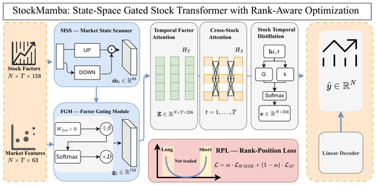
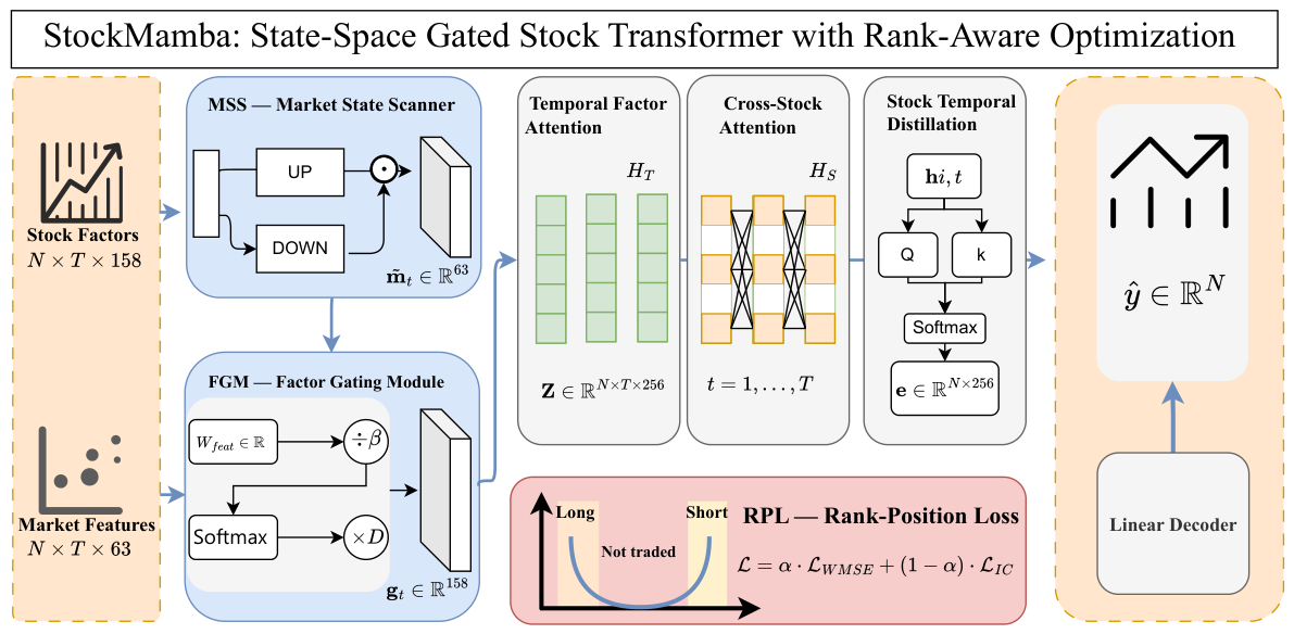
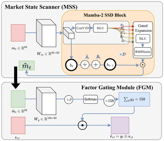
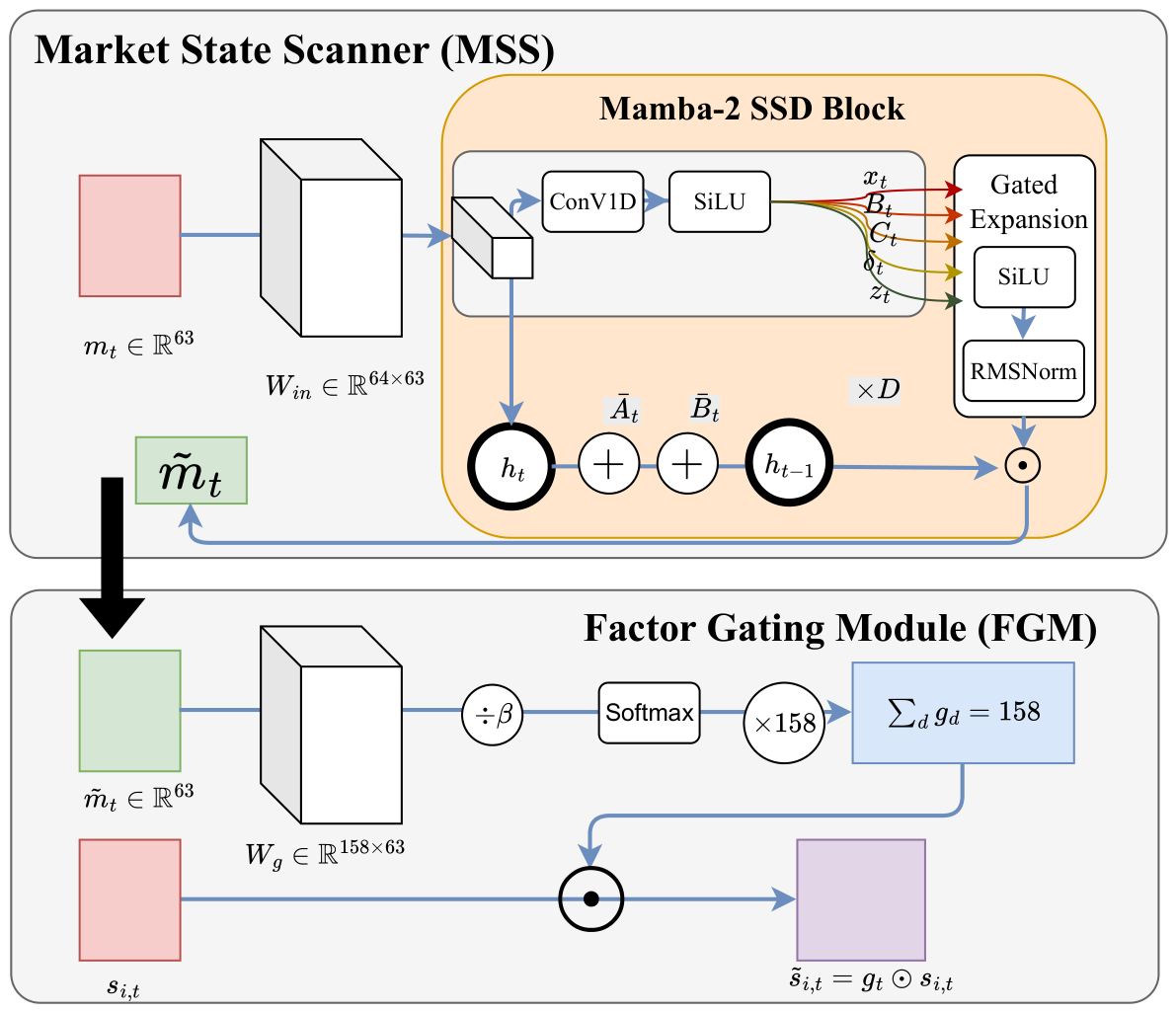
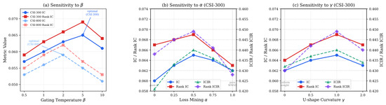
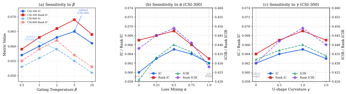
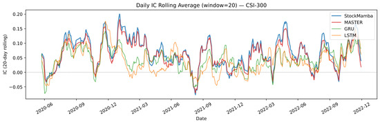
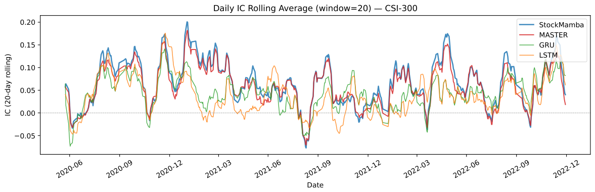
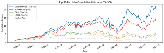
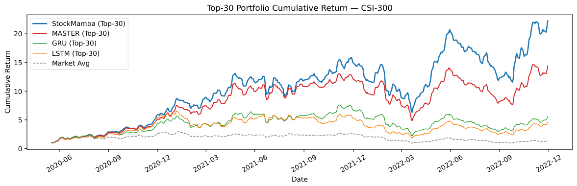

Disclaimer/Publisher’s Note: The statements, opinions and data contained in all publications are solely those of the individual author(s) and contributor(s) and not of MDPI and/or the editor(s). MDPI and/or the editor(s) disclaim responsibility for any injury to people or property resulting from any ideas, methods, instructions or products referred to in the content. |
© 2026 by the author. Licensee MDPI, Basel, Switzerland. This article is an open access article distributed under the terms and conditions of the Creative Commons Attribution (CC BY) license.