Article

Compact Orbits and Topological Sensitivity on Locally Compact Spaces


1
Rajagiri School of Engineering and Technology, Kakkanad 682039, Kerala, India
2
Sacred Heart College, Thevara, Kochi 682013, Kerala, India
3
APJ Abdul Kalam Technological University (KTU), Thiruvananthapuram 695016, Kerala, India
4
Muthoot Institute of Technology and Science, Kochi 682308, Kerala, India
*
Author to whom correspondence should be addressed.
Mathematics 2026, 14(10), 1752; https://doi.org/10.3390/math14101752
Submission received: 10 March 2026 / Revised: 8 May 2026 / Accepted: 14 May 2026 / Published: 19 May 2026

Abstract

We introduce a cover-based formulation of topological sensitivity and sensitivity at a point for continuous self-maps on locally compact spaces, extending the classical metric framework. Using the one-point compactification, we analyze the basin of attraction of infinity and relate it to escaping dynamics. We study the set K ( f ) consisting of points whose forward orbits are contained in a compact subset of the phase space, establishing its fundamental topological properties under suitable assumptions on the map f. In particular, we show that for proper maps, K ( f ) coincides with the complement of the escaping set. Under additional hypotheses on f, we prove that the boundary of the set of points with compact orbits, the boundary of the basin of attraction of infinity, and the set of sensitive points coincide. This provides a topological generalization of the classical dichotomy between Fatou and Julia sets in complex dynamics.

1. Introduction

The study of dynamical systems on non-compact spaces presents significant challenges that are absent in compact settings. In particular, distinguishing between bounded and unbounded orbit behavior requires tools that go beyond classical techniques in topological dynamics. While much of the existing theory has been developed for compact phase spaces, many naturally occurring systems [1,2], such as polynomial iterations [3,4,5], translation maps [6], and systems exhibiting escape to infinity, are inherently defined on locally compact but non-compact spaces.
A standard method to analyze such systems is to embed the space X into its one-point compactification X ^ = X { } . This allows escaping orbits to be interpreted as convergent sequences tending to the point at infinity, thereby enabling the use of compactness arguments [7]. Within this framework, two dynamically significant sets arise naturally:
1.
The set K ( f ) , consisting of points whose forward orbits are contained in a compact subset of X;
2.
The basin of attraction A ( ) , consisting of points whose orbits escape to infinity.
These sets are aanalogous to the filled Julia set and the basin of attraction of infinity in complex dynamics [8]. However, unlike the classical theory of rational maps on the Riemann sphere [9], our setting is purely topological and does not rely on any analytic or metric structure.
Recent developments in topological dynamics have emphasized the extension of chaotic concepts—such as sensitivity [10,11]—to non-metric and non-compact spaces. In particular, the notion of sensitivity has been generalized using open covers and purely topological formulations [12,13,14,15]. This motivates the introduction of a cover-based notion of topological sensitivity suitable for locally compact spaces.
The main contributions of this work are summarized as follows.
1.
We systematically study the set K ( f ) , establishing its invariance properties, structural characterizations, and topological nature under various assumptions on the map f.
2.
Using the one-point compactification, we show that for proper maps, K ( f ) = X A ( ) , thereby providing a precise topological dichotomy between bounded and escaping behavior.
3.
We introduce a cover-based notion of topological sensitivity and establish its relationships with global dynamical sets. Under suitable conditions, we prove that K ( f ) , A ( ) , and the set of sensitive points coincide, extending the classical Julia–Fatou dichotomy.
4.
Our results hold in general locally compact Hausdorff spaces, including non-metrizable spaces, thereby significantly broadening the scope of existing theories.
Section 2 reviews background material on Julia sets and sensitivity. Section 3 presents motivating examples. Section 4 develops the theory of compact orbits. Section 5 studies the basin of attraction of infinity. Section 6 introduces topological sensitivity and establishes its connection with the previously defined invariant sets.

2. Preliminaries

In this section, we collect the necessary material and establish the conceptual foundations for the subsequent development. We begin with a brief overview of Julia sets from complex dynamics, emphasizing their role as invariant sets exhibiting chaotic behavior. These classical results motivate the study of aanalogous structures from complex dynamics in a more general topological setting. The purpose of this section is to provide a brief history of complex dynamics, to describe some properties of Julia sets and to give some examples of Julia sets.

2.1. Historical Development of Julia Sets

The study of Julia sets originated in the early investigations of iteration theory in complex analysis during the first decades of the twentieth century. The subject was developed independently by Gaston Julia and Pierre Fatou, whose pioneering work between 1917 and 1920 initiated the systematic study of the dynamics of rational functions on the Riemann sphere C ^ [16,17].
Given a rational map f : C ^ C ^ of a degree of at least two, Julia and Fatou observed that the qualitative behavior of the iterates { f n } n 1 naturally divides the phase space into two invariant regions. The first region, later known as the Fatou set F ( f ) , consists of points where the iterates behave in a stable and regular manner. Its complement, the Julia set J ( f ) , consists of points where arbitrarily small perturbations lead to significantly different dynamical behavior. This dichotomy marked one of the earliest rigorous distinctions between regular and chaotic behavior in deterministic systems.
Gaston Julia focused on the geometric and topological complexity of the unstable set J ( f ) , establishing its complete invariance under f and demonstrating that it often forms highly irregular, infinitely detailed structures [16]. In parallel, Pierre Fatou developed powerful analytical tools based on normal family theory, proving fundamental results concerning the structure and classification of components of F ( f ) and their boundaries [17]. Their combined contributions showed that the Julia set is either the entire Riemann sphere or a perfect, nowhere dense subset of it.
Following this early period, research activity in complex dynamics slowed considerably for several decades. A renewed interest arose in the late twentieth century, largely motivated by computational experiments and visualizations. In particular, the work of Benoît Mandelbrot revealed the striking self-similar geometry of Julia sets associated with quadratic polynomials and uncovered their intimate relationship with the Mandelbrot set [18]. These discoveries played a crucial role in popularizing the subject and highlighting its relevance to fractal geometry and nonlinear science.
The modern mathematical framework of Julia sets was further strengthened by the seminal work of Douady and Hubbard, who introduced polynomial-like mappings and developed renormalization techniques to analyze local and global properties of complex dynamical systems [3]. Their results clarified the topological organization of Julia sets and established deep connections between local dynamics and global parameter spaces.
Today, Julia sets are regarded as fundamental examples of chaotic invariant sets in holomorphic dynamics. They exhibit characteristic features of chaos, including topological transitivity, dense periodic points, and sensitivity to initial conditions. As such, they continue to play a central role in contemporary research, linking complex analysis with ergodic theory, fractal geometry, and the general theory of dynamical systems.

2.2. Basic Properties of Julia Sets

Let f : C ^ C ^ be a rational map of degree d 2 . The Julia set J ( f 1 ) plays a central role in the qualitative description of the dynamics generated by the iterates of f. We summarize below some of its fundamental properties that are well established in the literature [3,4,5,8,9,16,17].
1.
The Julia set J ( f ) is completely invariant under the action of f, that is, f ( J ( f ) ) = J ( f ) = f 1 ( J ( f ) ) [4,5].
2.
J ( f ) is a closed subset of C ^ and hence compact [4,5].
3.
J ( f ) is a perfect set; i.e., it is closed and has no isolated points [4,5].
4.
The map f exhibits sensitive dependence on initial conditions; i.e., there exists δ > 0 such that for any open set U and for any point x U , there exists a point y U and an integer k 1 such that d ( f k ( x ) , f k ( y ) ) > δ . The positive number δ is called a sensitivity constant.
The dynamics restricted to the Julia set exhibit sensitive dependence on initial conditions. More precisely, for any z J ( f ) and any neighborhood U of z, there exists w U and an integer n 1 such that the spherical distance between f n ( z ) and f n ( w ) exceeds a fixed positive constant. Sensitivity is a hallmark of chaotic dynamics [2,8].
5.
The map f is topologically transitive on its Julia set; i.e., for any pair of non-empty open subsets U , V J ( f ) , there exists an integer n 1 such that f n ( U ) V . Transitivity ensures that the orbit of a typical point in the Julia set is distributed throughout the entire set [19].
6.
The Julia set coincides with the boundary of every Fatou component. In particular, if U is a connected component of the Fatou set, then U = J ( f ) .
This boundary characterization emphasizes the role of the Julia set as the interface between stable and unstable dynamics and underscores its significance as the locus of chaotic behavior [4].
7.
J ( f ) is the boundary of the basin of attraction of ∞; i.e., J ( f ) = A ( ) [8,19].
8.
J ( f ) = { z C ^ O f ( z ) } is bounded , where O f ( z ) is the orbit of z = { z , f ( z ) , f 2 ( z ) , } [8].

3. Examples of Julia Sets

We present several classic examples of Julia sets arising from polynomial and rational maps. These examples illustrate the wide variety of geometric and dynamical behaviors exhibited by Julia sets.

3.1. Quadratic Polynomial f ( z ) = z 2

Consider the map f ( z ) = z 2 . In this case, the Fatou set consists of two invariant components: the basin of attraction of 0 and the basin of attraction of ∞. The Julia set is given explicitly by J ( f ) = { z C | z | = 1 } , the unit circle. On J ( f ) , the dynamics are conjugated to the angle-doubling map on the circle, which is expanding and chaotic. This example demonstrates that Julia sets can be smooth manifolds, although this is exceptional among polynomial maps [4,8].

3.2. Quadratic Polynomial f ( z ) = z 2 2

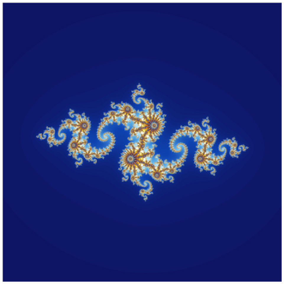
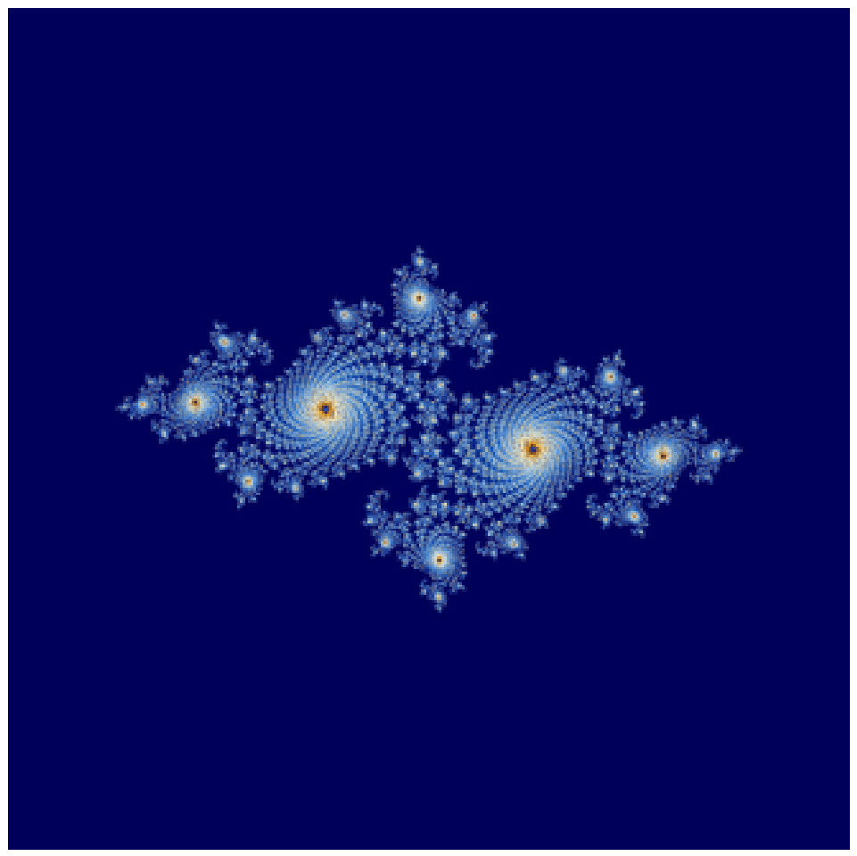
For the polynomial f ( z ) = z 2 2 , the Julia set is the real interval J ( f ) = [ 2 , 2 ] . Despite its simple geometric appearance; the dynamics on this set are highly chaotic. The restriction of f to [ 2 , 2 ] is topologically conjugate to the tent map and hence exhibits sensitive dependence on initial conditions and dense periodic points [2,8] (see Figure 1, Figure 2 and Figure 3).

3.3. Quadratic Polynomial f ( z ) = z 2 + i

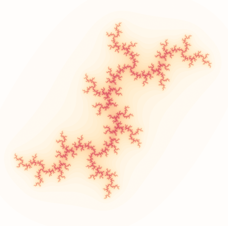
For f ( z ) = z 2 + i , the Julia set is connected but has a highly intricate fractal structure. It is neither smooth nor locally connected at many points. This example highlights how small changes in the parameter c can dramatically alter the topology and geometry of the Julia set [3,8].

3.4. Rational Map f ( z ) = z + 1 z

Consider the rational function f ( z ) = z + 1 z . The Julia set of this map is the real line together with the point at infinity. The dynamics exhibit strong expansion away from critical points, and the Julia set forms the boundary between regions of regular and chaotic behavior [4].

3.5. Lattès Maps

Lattès maps arise from affine transformations on complex tori projected onto the Riemann sphere. The Julia set of a Lattès map is the entire Riemann sphere C ^ . These examples are distinguished by the fact that chaotic behavior occurs everywhere, with no nontrivial Fatou components [6,8].
One example is the map f ( z ) = ( z 2 + 1 ) 2 4 z ( z 2 1 ) .
Remark 1.
An interesting and nontrivial connection between discrete dynamical systems and complex dynamics arises in the context of the Collatz conjecture, an unsolved problem in number theory. The classical formulation and dynamical aspects of the Collatz problem are well documented in [20,21].
Recent developments suggest that the behavior of the Collatz iteration can be interpreted through a topological and dynamical framework exhibiting structural similarities with Julia sets.
Consider the classical Collatz map f : N N defined by
f ( n ) = n 2 if n is even , 3 n + 1 2 if n is odd .
The Collatz conjecture asserts that for every N N , the forward orbit under f eventually enters the cycle { 1 , 2 , 4 } [20,21].
A topological interpretation of this problem has been proposed via the construction of a topological space ( N , τ f ) , where the topology τ f is generated by the Collatz map [22]. In this setting, the validity of the Collatz conjecture can be related to the connectivity of this space, which in turn is associated with properties such as upper τ f -boundedness and the failure of the weak- R 0 separation property [21].
This discrete dynamical structure admits a natural extension to the complex plane through holomorphic functions that interpolate the Collatz map. Such extensions have been studied in [22,23]. In particular, consider the function f 1 ( z ) = 1 4 2 z + 1 ( 2 z + 1 ) cos ( π z ) , which satisfies f ( n ) = f 1 ( n ) for all integers n N .
From the perspective of complex dynamics, the associated Julia set J ( f 1 ) plays a crucial role in separating stable and unstable dynamical behaviors. In aanalogy with the classical theory of rational maps (see [4,8]), the Fatou set corresponds to regions where the dynamics is regular, while the Julia set forms the boundary of chaotic behavior.
The connection with the Collatz conjecture can be interpreted heuristically as follows:
  • If the Collatz conjecture holds, all integer orbits are eventually attracted to the cycle { 1 , 2 , 4 } , suggesting that the integers lie within a global basin of attraction contained in the Fatou set.
  • The Julia set J ( f 1 ) then acts as a boundary separating this basin from escaping or chaotic dynamics in the complex plane.
  • The absence of the weak- R 0 property in the discrete topological model may be viewed as reflecting the non-existence of additional attractors or wandering domains that would allow integer orbits to diverge from the main cycle.
Thus, the connectivity of the discrete space ( N , τ f ) admits a natural analog in the topological structure of the Julia set, reinforcing the idea that the Collatz conjecture can be interpreted as a statement about the global organization of dynamical behavior.
This correspondence provides a conceptual bridge between number theory and complex dynamics and supports the broader interpretation of Julia sets as boundaries governing stability and chaos in dynamical systems.

4. Orbits with Compact Support

In this section, motivated by Property 8 of the Julia set given in the previous section, we introduce and systematically study the set K ( f ) of points whose orbits are contained in a compact subset of the phase space, which is equivalent to boundedness in C ^ . We begin by defining this set precisely and establishing its fundamental invariance property. We then define several equivalent characterizations of K ( f ) , including representation in terms of inverse images of compact sets. Under additional assumptions such as properness of the map, we investigate topological properties of K ( f ) , including closedness and local compactness. We also examine how the structure of K ( f ) depends on the underlying topology and metric, supported by illustrative examples, including non-metrizable spaces. This section lays the groundwork for understanding the interplay between bounded dynamics and escape phenomena.
Definition 1.
Let X be a non-compact locally compact Hausdorff space, and let f : X X be continuous. Define K ( f ) = { x X O f ( x ) C for some compact subset C X } , where O f ( x ) = { x , f ( x ) , f 2 ( x ) , f 3 ( x ) , } .
Definition 2.
Let X be a topological space and let f : X X be continuous. A subset A X is said to be forward invariant under f if f ( A ) A and is backward invariant if f 1 ( A ) A .
Definition 3 (Completely Invariant Set).
Let X be a topological space and let f : X X be a map. A subset A X is said to be completely invariant under f if f ( A ) = A = f 1 ( A ) .
Remark 2.
A set is completely invariant if and only if it is both forward and backward invariant.
Proposition 1.
Let X be a topological space and let f : X X be continuous. Then K ( f ) is forward invariant; i.e., f ( K ( f ) ) K ( f ) .
Proof. 
Let x K ( f ) . Then, O f ( x ) K for some compact subset K. Therefore { x , f ( x ) , f 2 ( x ) , f 3 ( x ) , } K . Hence { f ( x ) , f 2 ( x ) , f 3 ( x ) , } K . So O f ( f ( x ) ) K .
Hence K ( f ) is forward invariant. □
The following result shows that the boundary of the compact-orbit set exhibits strong dynamical invariance properties.
Proposition 2.
Let X be a locally compact Hausdorff space and let f : X X be a homeomorphism. Then the boundary of K ( f ) , denoted by K ( f ) , is completely invariant under f; that is, f K ( f ) = K ( f ) = f 1 K ( f ) .
Proof. 
Step 1: K ( f ) is completely invariant.
Forward invariance. Let x K ( f ) . Then there exists a compact set C X such that f n ( x ) C for all n 0 . For f ( x ) we have f n ( f ( x ) ) = f n + 1 ( x ) C , so the forward orbit of f ( x ) is also contained in C. Hence f ( x ) K ( f ) , and therefore f ( K ( f ) ) K ( f ) .
Backward invariance. Let x K ( f ) and let C be a compact set containing the forward orbit of X. Since f is a homeomorphism, f 1 is continuous and f 1 ( C ) is compact. For n 1 , f n ( f 1 ( x ) ) = f n 1 ( x ) C , and for n = 0 , f 0 ( f 1 ( x ) ) = f 1 ( x ) f 1 ( C ) . Hence O f ( f 1 ( x ) ) C f 1 ( C ) , which is compact. Thus f 1 ( x ) K ( f ) , so f 1 ( K ( f ) ) K ( f ) .
Combining both inclusions, f ( K ( f ) ) = K ( f ) = f 1 ( K ( f ) ) .
Step 2: Closure and interior are invariant.
Since f is a homeomorphism, for any subset A X , f ( A ¯ ) = f ( A ) ¯ , f ( A ) = ( f ( A ) ) . Applying this to A = K ( f ) and using the invariance of K ( f ) , f ( K ( f ) ¯ ) = K ( f ) ¯ , f ( K ( f ) ) = K ( f ) .
Step 3: Invariance of the boundary.
Recall that K ( f ) = K ( f ) ¯ K ( f ) . Since f is bijective, f ( A B ) = f ( A ) f ( B ) for all subsets A , B X . Therefore, f ( K ( f ) ) = f ( K ( f ) ¯ K ( f ) ) = f ( K ( f ) ¯ ) f ( K ( f ) ) . Using Step 2, f ( K ( f ) ) = K ( f ) ¯ K ( f ) = K ( f ) .
Step 4: Backward invariance of the boundary.
Since f is bijective and f ( K ( f ) ) = K ( f ) , applying f 1 gives f 1 ( K ( f ) ) = K ( f ) .
Hence, f ( K ( f ) ) = K ( f ) = f 1 ( K ( f ) ) . □
Proposition 3.
Let X be a topological space and let f : X X be continuous. Then
K ( f ) = C K ( X ) n 0 f n ( C ) ,
where K ( X ) denotes the family of compact subsets of X.
Proof. 
Let x K ( f ) . Then there exists a compact set C X such that f n ( x ) C for all n 0 . This implies that x f n ( C ) for all n 0 , and hence
x n 0 f n ( C ) .
Therefore,
x C K ( X ) n 0 f n ( C ) .
Next, let x C K ( X ) n 0 f n ( C ) . Then there exists a compact set C X such that
x n 0 f n ( C ) .
Hence f n ( x ) C for all n 0 , which implies that the forward orbit of x is contained in the compact set C. Therefore, x K ( f ) .
This completes the proof. □
Next, we prove some topological properties of K ( f ) .
Definition 4.
A topological space is said to be σ-compact if it can be written as a countable union of compact subsets.
Definition 5.
A subset of a topological space is called an F σ set if it is a countable union of closed sets.
Definition 6.
A subset of a topological space is called a G δ set if it is a countable intersection of open sets.
Proposition 4.
If X is locally compact Hausdorff and σ-compact and f : X X is continuous, then K ( f ) is an F σ subset of X.
Proof. 
Let ( C m ) m 1 be a compact exhaustion of X; that is, each C m is compact, C m C m + 1 , and
X = m 1 C m .
We show that
K ( f ) = m 1 n 0 f n ( C m ) .
First, let x K ( f ) . Then there exists a compact set C X such that O f ( x ) C . Since C m 1 C m and C is compact, there exists m 1 such that C C m . Hence f n ( x ) C m for all n 0 , and therefore
x n 0 f n ( C m ) .
Secondly, let x n 0 f n ( C m ) for some m. Then f n ( x ) C m for all n 0 , so the forward orbit of x is contained in the compact set C m . Hence x K ( f ) .
Thus,
K ( f ) = m 1 n 0 f n ( C m ) .
Finally, since each C m is compact and f is continuous, each set f n ( C m ) is closed. Therefore, n 0 f n ( C m ) is closed, and hence K ( f ) is a countable union of closed sets. Consequently, K ( f ) is an F σ subset of X. □
Definition 7.
Let X and Y be topological spaces and let f : X Y be a continuous map. The map f is said to be proper if for every compact set K Y , the preimage f 1 ( K ) is compact in X.
Proposition 5.
Let X be a non-compact locally compact Hausdorff space, and let f : X X be a continuous proper map. Then K ( f ) is closed in X.
Proof. 
To analyze compactness properties, we use the one-point compactification, which allows escaping behavior to be interpreted as convergence to infinity.
Let X ^ = X { } be the one-point compactification. Since f is proper, it extends to a continuous map f ^ : X ^ X ^ with f ^ ( ) = .
Define the escaping set I ( f ) = { x X f ^ n ( x ) in X ^ } . Claim 1: I ( f ) is open in X. Let x I ( f ) . Choose a neighborhood U of ∞ such that f ^ ( U ) U (which exists by continuity of f ^ at ∞ and f ^ ( ) = ). Since f ^ n ( x ) , there exists N such that f ^ n ( x ) U . By continuity of f ^ N , there is a neighborhood W of X with f ^ N ( W ) U . Then for every y W and every k 0 , f ^ N + k ( y ) f ^ k ( U ) U , so f ^ n ( y ) ; i.e., W I ( f ) .
Claim 2: K ( f ) = X I ( f ) . If x I ( f ) , then the orbit eventually leaves every compact subset of X, so O f ( x ) cannot be contained in any compact subset; hence x K ( f ) .
Conversely, if x I ( f ) , then ∞ is not a limit point of { f ^ n ( x ) } in the compact space X ^ . Therefore the orbit O f ( x ) in X ^ is contained in a compact subset of X ^ , so the orbit in X is compact and x K ( f ) .
Thus K ( f ) = X I ( f ) , and since I ( f ) is open, K ( f ) is closed. □

4.1. Note: Closedness of K ( f ) May Fail Without Local Compactness

Let X = R and Q R with the subspace topology, which is not locally compact, and define f ( x ) = x , the identity map. Then for any x Q , O f ( x ) = { x } , which is compact. Hence K ( f ) = Q , but Q is not closed in R .
Proposition 6.
Let X be a locally compact Hausdorff space and f : X X continuous. If K ( f ) X is closed, then K ( f ) is locally compact (and Hausdorff). In particular, if X is non-compact and f is proper, then K ( f ) is locally compact.
Proof. 
Since K ( f ) is closed in the Hausdorff space X, it is Hausdorff. Let x K ( f ) . Choose an open neighborhood U X of X with U ¯ compact (local compactness of X). Then U K ( f ) is an open neighborhood of X in K ( f ) and U K ( f ) ¯ U ¯ K ( f ) , which is compact as a closed subset of the compact set U ¯ . Hence K ( f ) is locally compact.
If f is proper and X is non-compact, locally compact Hausdorff, then K ( f ) is closed by Proposition 5 and hence locally compact. □
Proposition 7.
K ( f ) is the largest forward invariant subset of X on which f acts as a proper map.
Proof. 
First, K ( f ) is forward invariant. Moreover, f | K ( f ) is proper: if C K ( f ) is compact, then C is compact in X, and ( f | K ( f ) ) 1 ( C ) = K ( f ) f 1 ( C ) is compact as a closed subset of the compact set f 1 ( C ) .
Now let Y X be forward invariant and assume f | Y is proper. Fix y Y . Choose a compact neighborhood C of Y in Y. Then each ( f | Y ) n ( C ) is compact, and hence their intersection is compact and contains Y. Thus f n ( y ) C for all N 0 , so O f ( y ) C and y K ( f ) . Hence Y K ( f ) . □
Proposition 8.
Let X be a topological space and let f : X X be a homeomorphism. Then K ( f ) is completely invariant under f.
Proof. 
The forward invariance follows from Proposition 1.
Let x K ( f ) . Then there exists a compact set C X such that f n ( x ) C for all n 0 . Since f is a homeomorphism, f 1 is continuous and hence f 1 ( C ) is compact.
For n 1 , f n ( f 1 ( x ) ) = f n 1 ( x ) C , and for n = 0 , f 0 ( f 1 ( x ) ) = f 1 ( x ) f 1 ( C ) . Hence O f + ( f 1 ( x ) ) C f 1 ( C ) , which is compact. Therefore f 1 ( x ) K ( f ) , and so f 1 ( K ( f ) ) K ( f ) .
Combining both inclusions, we obtain f ( K ( f ) ) = K ( f ) = f 1 ( K ( f ) ) . Hence K ( f ) is completely invariant under f. □
Proposition 9.
Let h : X Y be a homeomorphism, and let f : X X and g : Y Y be continuous maps such that h f = g h ; then, h ( K ( f ) ) = K ( g ) .
Proof. 
Let x K ( f ) . Then there exists a compact subset C X such that f n ( x ) C , n 0 . Since h f = g h , we have g n ( h ( x ) ) = h ( f n ( x ) ) , n 0 . Hence, g n ( h ( x ) ) h ( C ) , n 0 . Because h is a homeomorphism and C is compact, the set h ( C ) is compact in Y. Hence, O g ( h ( x ) ) h ( C ) , which implies that h ( x ) K ( g ) . Consequently, h ( K ( f ) ) K ( g ) . Applying the same argument to the homeomorphism h 1 : Y X , we obtain K ( g ) h ( K ( f ) ) . Therefore, h ( K ( f ) ) = K ( g ) .
Proposition 10.
The boundary of K ( f ) has an empty interior; i.e., ( K ( f ) ) = .
Proof. 
Recall that for any subset A X , A = A ¯ A . Since K ( f ) K ( f ) ¯ , we obtain K ( f ) X K ( f ) . Assume, for contradiction, that ( K ( f ) ) . Then there exists a nonempty open set U K ( f ) . Because U K ( f ) K ( f ) , every point of U belongs to K ( f ) . Since U is open, this implies U K ( f ) . On the other hand, from K ( f ) X K ( f ) , we obtain U K ( f ) = . This contradicts the fact that U K ( f ) . Therefore, ( K ( f ) ) = . Hence the boundary K ( f ) has an empty interior. □

4.2. Some Examples

We will have some examples for a two-variable function for which K ( f ) is a single point, i.e., 0-dimensional, and R , i.e., 1-dimensional.
For x = ( x 1 , x 2 ) and y = ( y 1 , y 2 ) , let f : R 2 R 2 be defined by f ( x , y ) = ( 2 x , 2 y ) .
1.
Let d 1 ( x , y ) = ( x 1 y 1 ) 2 + ( x 2 y 2 ) 2 ; then clearly K ( f ) = { ( 0 , 0 ) } .
2.
Let d 2 ( x , y ) = | x 1 y 1 | + | x 2 y 2 | ; then K ( f ) = { ( 0 , 0 ) } .
3.
Let d 3 ( x , y ) = max { | x 1 y 1 | ; | x 2 y 2 | } , then K ( f ) = { ( 0 , 0 ) } .
4.
Let φ : R 2 R × ( 1 , 1 ) by φ ( x , y ) = ( x , tanh ( y ) ) ; then φ is a homeomorphism. Let d 4 ( p , q ) = | | φ ( p ) φ ( q ) | | 2 , f n ( x , y ) = ( 2 n x , 2 n y ) ; then φ ( f n ( x , y ) ) = ( 2 n x , tanh ( 2 n y ) . Then K ( f ) = { ( 0 , y ) y R } , which is the y -axis.
5.
Define d 5 ( x , y ) = | arctan ( x ) arctan ( y ) | .
Since arctan : R ( π 2 , π 2 ) is a homeomorphism onto a bounded interval, the metric space ( R , d 5 ) is bounded.
Moreover, every closed and bounded subset of ( π 2 , π 2 ) is compact, and compactness in ( R , d 5 ) corresponds to compactness in that interval.
Now observe that arctan ( 2 n x ) π 2 , π 2 for all n .
Hence the set { arctan ( 2 n x ) : n 0 } is bounded in a compact interval and therefore relatively compact in ( R , d 5 ) .
Thus every orbit is relatively compact in d 5 , and so K d 5 ( f ) = R .
The set K ( f ) depends crucially on the choice of metric and therefore on the induced topology.
Proposition 11.
Let d 1 and d 2 be two equivalent metrics on a set X; that is, they induce the same topology on X. Then a subset C X is compact with respect to d 1 if and only if it is compact with respect to d 2 . Consequently, for any continuous map f : X X , K d 1 ( f ) = K d 2 ( f ) , where K d i ( f ) denotes the set of points whose forward orbits are relatively compact with respect to the metric d i .
Proof. 
Since d 1 and d 2 induce the same topology on X, the identity map id : ( X , d 1 ) ( X , d 2 ) is a homeomorphism, and its inverse is again the identity map. It is a standard topological fact that homeomorphisms preserve compactness [24].
Let C X be compact in ( X , d 1 ) . Because id : ( X , d 1 ) ( X , d 2 ) is continuous, the image id ( C ) = C is compact in ( X , d 2 ) . Applying the same argument to the inverse identity map shows that compactness in ( X , d 2 ) implies compactness in ( X , d 1 ) . Hence the two metrics determine exactly the same compact subsets of X.
By definition, K d i ( f ) = x X { f n ( x ) } n 0 C for some compact set C X . Since the families of compact sets induced by d 1 and d 2 coincide, a forward orbit is relatively compact with respect to d 1 if and only if it is relatively compact with respect to d 2 . This proves that K d 1 ( f ) = K d 2 ( f ) .

4.3. Examples of K ( f ) on a Non-Metrizable Locally Compact Space

1.
Let X = I × R where I is a discrete index space and R is the usual metric.
Then X is locally compact, not compact, and non-metrizable.
(a)
We define f 1 : X X as f 1 ( i , t ) = ( i , t + 1 ) and f 1 n ( i , t ) = ( i , t + n ) ,
Then K ( f 1 ) = .
(b)
We set f 2 : X X by f 2 ( i , t ) = ( i , t / 2 )
Then f 2 n ( i , t ) = ( i , t / 2 n ) and K ( f 2 ) = X .
(c)
We define f 3 : X X by f 3 ( i , t ) = ( i , t / 2 ) if i J and f 3 ( i , t ) = ( i , t + 1 ) if i J , where J I . Then K ( f 3 ) = J × R .

4.4. Example to Show That K ( f ) Can Be Disconnected

1.
Let X = C [ 0 , 1 ] . We define d ( f , g ) = sup x X | | f ( x ) g ( x ) | | .
Let ψ : X X be defined as ψ ( f ) = f 2 , f X .
If | | f | | < 1 , then | | ψ n ( f ) | | 0 . If | | f | | = 1 then | | ψ n ( f ) | | = 1 and if | | f | | > 1 , then | | ψ n ( f ) | | .
Hence K ( ψ ) = { f | | f | | < 1 } { 1 , 1 } , therefore K ( ψ ) is disconnected.
2.
Let X = C ( S 1 ) , the space of smooth 2 π - periodic functions. Define d ( f , g ) = sup x [ 0 , 2 π ] | f ( x ) g ( x ) | .
Let ψ : X X be defined as ψ ( f ) = f , the derivative of f. Using Fourier Series, f ( x ) = k Z a k e i k x .
Hence ψ n ( f ) = k Z ( i k ) n a k e i k x . Therefore, the orbit of f lies in a finite dimensional space and hence is relatively compact. Therefore, K ( ψ ) = C ( S 1 ) .
3.
Let ω 1 be the first uncountable ordinal. Let ω < ω 1 . Let X = [ 0 , ω 1 ] × [ 0 , ω ] { ( ω 1 , ω 1 ) } , with the product order topology.
f : X X is defined as f ( α , n ) = ( α , n 1 ) , n > 0 ( α , 0 ) , n = 0 . Then K ( f ) = X .
Let g : X X be defined as g ( α , n ) = ( α , n ) n = 0 ( α + 1 , n ) n > 0 . .
Then K ( g ) = [ 0 , ω 1 ] × { 0 } .
These examples show that even in a non-metrizable locally compact space, the non-escaping set K ( f ) can range from empty to the entire space and can realize arbitrary subsets like vertical slices of the form J × R . The structure of K ( f ) is therefore highly sensitive to the dynamics along different components of the space.

5. Basin of Attraction of Infinity

In this section, we study the set of points whose orbits escape to infinity within the one-point compactification of the phase space. We define the escape set A ( ) and analyze its fundamental properties, topological structure, and its characterization as a G δ -set under suitable conditions. A central result of this section is the precise relationship between K ( f ) and A ( ) , showing that for proper maps these sets are complementary. We also provide examples demonstrating that certain properties, such as openness of A ( ) , depend critically on the properness of the map. This section establishes a clear dichotomy between compact orbit behavior and escape to infinity.
Definition 8.
Let X ^ = X { } be the one-point compactification of X. So we can extend the continuous function f : X X to X ^ by f ^ : X ^ X ^ as f ^ ( x ) = f ( x ) , x X and f ^ ( ) = . We define the basin of attraction of ∞ as A ( ) = { x X ^ f ^ n ( x ) } .
Such escaping behavior is closely related to the classical theory of Julia sets and has been extensively studied in recent literature [25,26,27].
In this section, unless otherwise specified, X is a locally compact Hausdorff space, and X ^ is the one-point compactification of X; i.e., X ^ = X { } , f : X X is continuous and f ^ is the extension of f to X ^ with f ^ ( ) = .
Proposition 12.
The basin of attraction of infinity A ( ) is non-empty; i.e., A ( ) .
Proof. 
Since f ^ ( ) = , we have f ^ n ( ) = for all n 0 . Hence, A ( ) . □
Proposition 13.
For every neighborhood U of ∞ in X ^ ,
A ( ) = N 0 n N f ^ n ( U ) .
In particular, A ( ) is a G δ subset of X ^ , and A ( ) X is a G δ subset of X.
Proof. 
Fix a neighborhood U of ∞. A point x X ^ satisfies f ^ n ( x ) if and only if there exists N such that f ^ n ( x ) U for all n N . Equivalently, x n N f ^ n ( U ) for some N. Taking the union over all N 0 yields the stated formula.
Since each f ^ n ( U ) is open (as U is open and f ^ is continuous), n N f ^ n ( U ) is a G δ , and the union over N is again a G δ . □
Proposition 14.
The set K ( f ) is contained in the complement of A ( ) ; i.e., K ( f ) X A ( ) .
Proof. 
Let x K ( f ) . By definition, O f ( x ) C for some compact subset C X .
Hence there exists a compact set C X such that f n ( x ) C for all n 0 . Suppose, on the contrary, that x A ( ) . Then, by the definition of the basin of attraction of ∞, for every compact set K X , there exists N N such that f n ( x ) K for all n N . Taking K = C , this contradicts the fact that f n ( x ) C for all n 0 .
Therefore x A ( ) , and hence x X A ( ) . Since X was arbitrary, we conclude that K ( f ) X A ( ) .
Proposition 15.
If f is proper, then K ( f ) = X A ( ) .
Proof. 
A point x X belongs to A ( ) if and only if its orbit eventually leaves every compact subset of X. This is equivalent to saying that x K ( f ) . Hence, K ( f ) = X A ( ) . □

5.1. An Example to Show That K ( f ) = X ^ A ( )

Let
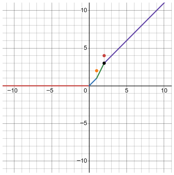
f ( x ) = 0 , x 0 x , 0 x 1 2 x 1 , 1 x 2 x + 1 , x 2 .
Clearly K ( f ) = ( , 2 ] , for x 2 , f n ( x ) , and hence A ( ) = ( 2 , ) .
Hence in this case K ( f ) = X A ( ) .
Proposition 16.
A ( ) is forward invariant subset of X ^ .
Proof. 
We have to prove that f ( A ( ) ) A ( ) .
Let x f ( A ( ) ) ,
x = f ( y ) for some y A ( ) .
f n ( y ) as n .
f n 1 ( f ( y ) ) as n . ⇒ f ( y ) A ( ) . That is, x A ( ) .
Hence f ( A ( ) ) A ( ) (see Figure 4) □
Proposition 17.
If f is proper, then A ( ) is open in X.
Proof. 
Let x A ( ) ; then f n ( x ) in X ^ = X { } .
Since the neighborhoods of ∞ in X ^ are of the form X ^ C , for some compact set C X , n N , f n ( x ) X ^ C , n N .
Hence f n ( x ) C , n N .
Let x A ( ) and let C X be compact. By the characterization of escape, there exists n 0 such that f n ( x ) C . Since f n is proper, the preimage f n ( C ) is compact. Thus X f n ( C ) is an open neighborhood of X consisting entirely of points whose N-th iterate lies outside C. Hence this neighborhood is contained in A ( ) . □

5.2. Example (Failure of Openness Without Properness)

If f is not proper, the preimage of a compact set may be non-compact. In this case, sequences of points arbitrarily close to an escaping point may have iterates that return to compact regions. Consequently, the set A ( ) need not be open.
Let X = R . Define the function f : X X by
f ( x ) = x + sin ( x 2 ) x + 1 .
The function f is continuous but not proper. Indeed, there exists a sequence ( x n ) with x n such that f ( x n ) remains bounded. Therefore, the preimage of a compact set under f need not be compact.
We show that the basin of attraction A ( ) is not open. Observe that
sin ( x 2 ) x + 1 0 as x .
Thus, f ( x ) behaves asymptotically like x, and for sufficiently large values of x, the iterates f n ( x ) tend to + . Such points therefore belong to A ( ) .
However, the oscillatory behavior of sin ( x 2 ) implies that there exist arbitrarily large values of x for which sin ( x 2 ) is close to 1 . In such cases, f ( x ) is less than x , and the forward iterates may return to bounded subsets.
Hence, there exist points in A ( ) that are arbitrarily close to points not belonging to A ( ) . It follows that A ( ) is not open.
This example shows that the properness assumption is essential for the openness of A ( ) .
Proposition 18.
The boundary K ( f ) is a closed, nowhere dense subset of X ^ .
Proof. 
Since K ( f ) is the boundary of a subset of X, it is closed.
Suppose that ( K ( f ) ) . Then there exists a nonempty open set U K ( f ) . Since K ( f ) = K ( f ) ¯ ( K ( f ) ) , it follows that U ( K ( f ) ) = . However, U K ( f ) ¯ , contradicting the definition of interior. Hence, ( K ( f ) ) = . So, K ( f ) is nowhere dense. □

5.3. Examples

For A ( ) on R . The following examples show that A ( ) can be the full space or empty.
1.
Let f : R R be defined by f ( x ) = x + 1 ; then A ( ) = R .
2.
Let f : R R be defined by f ( x ) = x / 2 ; then A ( ) = .
Proposition 19.
A point x A ( ) if and only if for every compact set C X , n 0 such that f n ( x ) C .
Proof. 
Suppose that x A ( ) . By definition, f ^ n ( x ) in the one-point compactification X ^ = X { } . Let C X be an arbitrary compact set. Then X ^ C is an open neighborhood of ∞ in X ^ . Since f ^ n ( x ) , there exists N 0 such that f n ( x ) X ^ C , n N . In particular, f N ( x ) C . Therefore, for every compact set C X , there exists n 0 such that f n ( x ) C .
Conversely, suppose that for every compact set C X , there exists n 0 such that f n ( x ) C . Let U be an arbitrary neighborhood of ∞ in X ^ . By the definition of the one-point compactification, there exists a compact set C X such that U = X ^ C . By assumption, there exists n 0 such that f n ( x ) C . Equivalently, f n ( x ) U . Hence, for every neighborhood U of ∞, there exists n 0 such that f n ( x ) U . Therefore, f ^ n ( x ) , which implies that x A ( ) . □

6. Sensitivity

This section is devoted to the study of sensitivity, a fundamental concept in the theory of chaotic dynamical systems. We begin by recalling the classical notion of metric sensitivity, which we mentioned in Section 2.2. We then introduce a cover-based formulation of topological sensitivity that is applicable in general to topological spaces, including non-metrizable settings. We analyze the structure of the set of sensitive points and establish several of its properties. The result of this section connects local instability with global dynamical behavior and prepares the ground for relating sensitivity to compact and escaping orbits in the overall framework of the paper.

6.1. Metric Sensitivity

Definition 9.
Let ( X , d ) be a metric space and let f : X X be continuous. We say that f is sensitive at x X if there exists δ > 0 such that for every neighborhood U of x, there exist y U and n N satisfying d ( f n ( x ) , f n ( y ) ) δ .
The number δ is called a sensitivity constant of f at x.
We define S ( f ) = { x X f is sensitive at x } . f is sensitive on X if S ( f ) = X .

6.1.1. Remark: Sensitivity Depends on the Chosen Metric (Not on the Orbit)

Let X = R , and let f ( x ) = x + 1 .
Let d 1 ( x , y ) = | x y | , ρ ( x , y ) = | e x e y | .
Then f is sensitive on ( R , ρ ) but not on ( R , d 1 ) .
If ( X , d ) is a compact metric space, the sensitivity is preserved within the class of equivalent metrics.

6.1.2. Examples

1.
It is well known that the tent map f : [ 0 , 1 ] [ 0 , 1 ] defined as
f ( x ) = 2 x 0 x 1 / 2 2 ( 1 x ) 1 / 2 x 1 is sensitive on [ 0 , 1 ] ; i.e., S ( f ) = [ 0 , 1 ] . [2].
2.
Let X = [ 1 , 1 ] and f : X X be f ( 1 / n ) = 1 n + 1 , f ( 0 ) = 0 , f ( 1 / n ) = 1 ( n 1 ) ; n 2 , f ( 1 ) = 1 . f is continuous on X.
If x X { 0 } , then f is not sensitive at x, since x is an isolated point. But for x = 0 , given ϵ > 0 , there exists y = 1 / n ( x ϵ , x + ϵ ) such that d ( f n ( x ) , f n ( y ) ) = d ( 0 , 1 ) = 1 .
Hence S ( f ) = { 0 } .
3.
Let f : C C be defined as f ( z ) = z 2 .
For z C with | z | < 1 , | f n ( z ) | 0 as n . For z C with | z | > 1 , | f n ( z ) | . If z , w C , with | z | < 1 and | w | < 1 , then | f n ( z ) f n ( w ) | | f ( z ) | + | f n ( w ) | 0 as n . So z S ( f ) .
If z , w C with | z | > 1 and | w | > 1 , then
| f n ( z ) f n ( w ) | = | z 2 n w 2 n | = | z | 2 n | 1 ( w z ) 2 n | . So z S ( f ) .
If | z | = 1 , then | f n ( z ) | = 1 , so z S ( f ) .
Hence, S ( f ) = S 1 , which is the Julia set of f.
Proposition 20.
Let ( X , d ) be a metric space and let f : X X be continuous. Then the set of sensitive points S ( f ) is forward invariant; that is, f S ( f ) S ( f ) [2,10].
Proposition 21.
Let ( X , d ) be a metric space and f : X X be continuous. Assume that the sensitive set S ( f ) is closed. If x S ( f ) , then O f ( x ) ¯ S ( f ) .
Proof. 
By Proposition 20, S ( f ) is forward invariant. Hence O f ( x ) S ( f ) and S ( f ) is closed, and we obtain
O f ( x ) ¯ S ( f ) .
Hence every point in the orbit closure of X is sensitive. □
Proposition 22.
The set of sensitive points S ( f ) is an F σ -set.
Proof. 
For a fixed δ > 0 , let S δ = { x X f is sensitive at x with sensitivity constant δ } .
We prove that S ( f ) = n Z + S 1 / n ( f ) ¯ .
We have S δ ( f ) ¯ S δ / 2 ( f ) S ( f ) .
n Z + S 1 / n ( f ) ¯ S ( f ) .
Let x S ( f ) . Then there exists n Z + such that x S δ ( f ) where δ > 1 / n (if δ < 1 / n , n Z + then i n f { δ | x S δ ( f ) } = 0 , contradicts x S ( f ) ).
So x S 1 / n ( f ) S 1 / n ( f ) ¯ .
Hence S ( f ) n Z + S 1 / n ( f ) ¯ . □
Generalizations of sensitivity in topological spaces were studied in [28] and more recently in the context of semiflows on general topological spaces in [29]. We define topological sensitivity at a point in non-metrizable topological spaces.
Definition 10.
Let X be a topological space and f : X X be continuous. f is topologically sensitive at a point x X with respect to an open cover U if for every neighborhood G of x, ∃ y G and 1 n Z + such that ( f n ( x ) , f n ( y ) ) U × U , U U .
In this case U is called a sensitivity cover of f at x.
If f is sensitive at every point of X with respect to U , we say that f is topologically sensitive on X, with respect to U .
Let S U ( f ) = { x X f is topologically sensitive at x with respect to open cover U } .
f is topologically sensitive on X with respect to open cover U S U ( f ) = X . Topological sensitivity continues to be an active area of research, with recent developments linking it to structural properties of dynamical systems [30,31].
Proposition 23.
The following statements are equivalent.
1. 
S U ( f ) = X .
2. 
For every non-empty open set G of X, there exist x , y G and n Z + such that ( f n ( x ) , f n ( y ) ) U × U , U U .
Proof. 
(1) ⇒ (2).
Assume S U ( f ) = X . Let G X be a non-empty open set. Choose x G . Since x S U ( f ) , by definition, for every neighborhood H of X, th/re exist y H and n N such that ( f n ( x ) , f n ( y ) ) U U U × U . Taking H = G , we obtain y G and n N with the required property. Thus (2) holds.
(2) ⇒ (1).
Assume (2). Let x X and let G be any open neighborhood of X. Since G is non-empty and open, by (2) there exist x 1 , y 1 G and n N such that ( f n ( x 1 ) , f n ( y 1 ) ) U U U × U .
We claim that X is sensitive. Since U U U × U is open in X × X , its complement is closed. Let φ n : X × X X × X , φ n ( a , b ) = ( f n ( a ) , f n ( b ) ) . Then φ n is continuous. Hence φ n 1 ( X × X ) U U U × U is closed in X × X .
Since ( x 1 , y 1 ) belongs to this closed set, there exists an open neighborhood W X × X of ( x 1 , y 1 ) such that φ n ( W ) ( X × X ) U U U × U . Because W is open in X × X , there exist open sets U 0 , V 0 X such that ( x 1 , y 1 ) U 0 × V 0 W . Since x G and x 1 , y 1 G , we may choose an open neighborhood G G with x G and G U 0 V 0 . Then for every y G , ( f n ( x ) , f n ( y ) ) U U U × U .
Thus X is topologically sensitive. Since X is arbitrary, S U ( f ) = X . □
Proposition 24.
Let X , d be a metric space and f : X X be continuous. Let T d denote the topology on X generated by metric d. Then if f is metrically sensitive on X, then f is topologically sensitive.
Proof. 
Let δ be a sensitive constant for f.
Let ϵ = δ 2 , then U = { B ϵ ( p ) p X } is a sensitivity cover for f. So if G is an open set in X and x G , then there exists y G , n Z + such that d ( f n ( x ) , f n ( y ) ) δ .
( f n ( x ) , f n ( y ) B ϵ ( p ) × B ϵ ( p ) , for every p X .
U is a sensitivity cover for f. Hence f is topologically sensitive. □
Proposition 25.
If ( X , d ) is compact then f is topologically sensitive 1071 f is metrically sensitive.
Proof. 
Let U be a sensitive cover for f and let ϵ be a Lebesgue number of U (since X is compact, every open cover has a Lebesgue number).
There exists ϵ > 0 such that if d ( a , b ) < ϵ , then a , b lie in some common U U .
Let G be any non- empty subset of X, By assumption, x , y G , n Z + such that ( f n ( x ) , f n ( y ) ) U U U × U . Hence, d ( f n ( x ) , f n ( y ) ) ϵ .
f is metrically sensitive. □

6.2. Example: Compactness in the Above Theorem Is Necessary

Example 1.
Let X = R equipped with the metric d ( x , y ) = tan 1 ( x ) tan 1 ( y ) . Note that d ( x , y ) π for all x , y R .
Define f : R R by f ( x ) = 2 x . Consider the open cover U = { ( , 1 ) , ( 2 , 2 ) , ( 1 , ) } of R . Let G R be a nonempty open interval. For any distinct points x , y G , f n ( x ) = 2 n x and f n ( y ) = 2 n y . As n , the points f n ( x ) and f n ( y ) eventually belong to different elements of the cover U . Hence, U is a sensitivity cover for f. Therefore, f is topologically sensitive.
Now suppose that f is metrically sensitive. Then there exists δ > 0 such that for every nonempty open set U R , there exist x , y U and n 0 satisfying d ( f n ( x ) , f n ( y ) ) > δ . However, d ( f n ( x ) , f n ( y ) ) = tan 1 ( 2 n x ) tan 1 ( 2 n y ) . Since tan 1 ( t ) π 2 as t , it follows that for sufficiently large n, tan 1 ( 2 n x ) and tan 1 ( 2 n y ) are both arbitrarily close to π 2 . Consequently, d ( f n ( x ) , f n ( y ) ) 0 as n . This contradicts metric sensitivity. Therefore, f is not metrically sensitive.
Proposition 26.
f is topologically sensitive iff f n is topologically sensitive.
Proof. 
If U is a sensitive cover for f n , then U is a sensitive cover for f.
Assume that U is a sensitivity cover for f. For every k { 0 , 1 , , n 1 } let U k = { f k ( U ) | U U } .
Let V be the joint of U 0 , U 1 , U k .
i.e., V = { U 0 f 1 ( U 1 ) f ( n 1 ) ( U n 1 ) | U k U } .
We now prove that V is a sensitivity cover for f n .
Let G be a non-empty open subset of X. Then there exist x , y G and Z + such that ( f ( x ) , f ( y ) ) U U U × U .
Let q Z + and 0 p < n be such that m = q n + p .
( ( f n ) q ( x ) , ( f n ) q ( y ) ) = ( f m p ( x ) , f m p ( y ) ) v V V × V .
Because if ( f m p ( x ) , f m p ( y ) ) V × V for some V = U 0 f 1 ( U 1 ) f ( n 1 ) ( U n 1 V , then ( f m ( x ) , f m ( y ) ) U p × U p , U p U , which is a contradiction.
So V is a sensitivity cover for f n .
Hence f n is topologically sensitive. □
Proposition 27.
Let f : X X be a continuous map. Then the set S U ( f ) is forward invariant under f; that is, f ( S U ( f ) ) S U ( f ) . Equivalently, if x S U ( f ) , then f ( x ) S U ( f ) .
Proof. 
Let x S U ( f ) .
Let f ( x ) G be open.
Then f 1 ( G ) is a neighborhood of x.
y f 1 ( G ) , n 1 with ( f n ( x ) , f n ( y ) ) u U U × U .
( f n ( f ( x ) , f n ( f ( y ) ) = ( f n + 1 ( x ) , f n + 1 ( y ) U U U × U .
Since f ( y ) G , f ( x ) is sensitive. □
Proposition 28.
Let f : X X be continuous. Then the set S U ( f ) is a forward invariant subset of X with respect to the sensitive cover U . Equivalently, if x S U ( f ) then f ( x ) S U ( f ) .
Proof. 
It follows from the above proposition. □
Proposition 29.
Let X be metrizable. Let V ϵ ( x 0 ) = { x X | d ( x , x 0 ) < ϵ } , U = { V ϵ ( x 0 ) | ϵ > 0 } . Then sensitivity with respect to U is equivalent to metric sensitivity at x.
Proof. 
Suppose first that f is metrically sensitive at x 0 . Then there exists δ > 0 such that for every neighborhood U of x 0 , there exist points x , y U and n 0 satisfying d ( f n ( x ) , f n ( y ) ) > δ . Let V = { V ϵ ( x 0 ) 0 < ϵ < δ / 2 } . If A X is any subset with diameter less than δ , then A cannot intersect two distinct elements of V . Indeed, if a , b A belong to distinct members of V , then d ( a , b ) δ , which contradicts the assumption that diam ( A ) < δ . Now let U be any neighborhood of x 0 . By metric sensitivity, there exist x , y U and n 0 such that d ( f n ( x ) , f n ( y ) ) > δ . Hence, the set { f n ( x ) , f n ( y ) } cannot be contained in a single element of V . Therefore, f is sensitive with respect to the family U at x 0 .
Conversely, suppose that f is sensitive with respect to U at x 0 . Then there exists ϵ > 0 such that for every neighborhood U of x 0 , there exist x , y U and n 0 for which the set { f n ( x ) , f n ( y ) } is not contained in any element of U . In particular, f n ( x ) V ϵ ( f n ( y ) ) , and therefore d ( f n ( x ) , f n ( y ) ) ϵ . Thus, f is metrically sensitive at x 0 . □
Proposition 30.
For every open cover U , the sensitive set S U ( f ) is forward invariant; that is,
f ( S u ( f ) ) S u ( f ) .
Proof. 
Let x S ( f ) and let U be an open neighborhood of f ( x ) . By continuity of f, there exists an open neighborhood W of X such that f ( W ) U . Since X is sensitive, there exist y W , N N , and an open cover V x of X such that
( f n ( x ) , f n ( y ) ) V × V for all V V x .
It follows that
( f n + 1 ( x ) , f n + 1 ( y ) ) V × V ,
showing that f ( x ) is topologically sensitive. Hence f ( S U ( f ) ) S U ( f ) . □

6.3. Examples Illustrating Topological Sensitivity

In this section we present explicit examples that clarify the definition of topological sensitivity introduced in the definition. These examples demonstrate both the presence and absence of sensitivity in purely topological terms.
1.
Let X = { 0 , 1 } N endowed with the product topology, and let f = σ : X X be the left shift defined by
σ ( ( x 0 , x 1 , x 2 , ) ) = ( x 1 , x 2 , x 3 , ) .
The space X is compact, totally disconnected, and metrizable, but the argument below is purely topological.
Result 1.
The shift map σ is topologically sensitive at every point of X. Hence
S ( σ ) = X .
Proof. 
Let x X and let U be any open neighborhood of X. Then U contains a basic cylinder set determined by a finite initial block of coordinates. Choose y U such that Y differs from X at some coordinate k outside this finite block.
Let V be the open cover of X consisting of cylinder sets determined by the first coordinate. Then σ k ( x ) and σ k ( y ) differ in the first coordinate and hence cannot lie in the same element of V . Thus
( σ k ( x ) , σ k ( y ) ) V × V for all V V .
Therefore σ is topologically sensitive at X. Since X was arbitrary, S ( σ ) = X . □
2.
Let X = S 1 and define f : X X by f ( z ) = z 2 .
Result 2.
The map f ( z ) = z 2 is topologically sensitive at every point of S 1 [19].
Proof. 
Let x S 1 and let U be any open arc containing X. Since f is expanding, there exists N N such that f n ( U ) covers the entire circle.
Let V be any finite open cover of S 1 by proper arcs. Then there exist y U such that f n ( x ) and f n ( y ) lie in distinct elements of V . Hence the sensitivity condition is satisfied at X. □
3.
Let X = R with the usual topology and define f ( x ) = x + 1 . then S ( f ) = .
Proof. 
Fix x R . Let V be the open cover of R consisting of unit intervals { ( k 1 , k + 1 ) : k Z } . For any neighborhood U of X and any y U , we have
f n ( y ) f n ( x ) = y x for all n N .
Hence f n ( x ) and f n ( y ) always remain in the same element of V . Therefore the sensitivity condition fails at X. □
4.
Let X be any topological space and define f : X X by f ( x ) = p for a fixed point p X , then f is not topologically sensitive.
Proof. 
For every x X and every N N , f n ( x ) = p . Hence for any open cover V of X, there exists V V such that p V , and therefore
( f n ( x ) , f n ( y ) ) V × V for all y X and all n .
Thus the sensitivity condition cannot be satisfied at any point. So S u ( f ) = . □
Remark 3.
The above examples show that topological sensitivity captures genuine chaotic behavior. Expanding and shift-type systems exhibit sensitivity at every point, while equicontinuous or rigid systems fail to exhibit sensitivity anywhere.
Topological sensitivity continues to be an active area of research, with recent developments linking it to structural properties of dynamical systems [32].

7. Relation Between K ( f ) and A (∞)

In this section, we prove that under some assumptions on f, the complement of K ( f ) , A ( ) and S u ( f ) are equal.
Throughout this section, X is a locally compact, Hausdorff space, X ^ = X { } , f : X X is continuous and f ^ : X ^ X ^ is an extension of f with f ( ) = .
Proposition 31.
If f is a proper map, then A ( ) = K ( f ) .
Proof. 
Since A ( ) = X K ( f ) , A ( ) = A ( ) ¯ K ( f ) ¯ = K ( f ) .
Suppose x K ( f ) . Then there are two possibilities: x ( K ( f ) ) 0 or x ( X K ( f ) ) 0 .
Case 1
Let x ( K ( f ) ) 0 open neighborhood G of x , such that G K ( f )
a compact set C X such that O f ( y ) C , y G .
Fix any V U . Since f n is continuous and C is compact, { f n / C n 0 } is equicontinuous on C.
Hence, ∃ a neighborhood G 0 G of x such that ( f n ( x ) , f n ( y ) ) V × V , y G 0 , n 0 .
Hence f is not sensitive at x.
Case 2
Let x ( X K ( f ) ) 0 open neighborhood G of x such that G ( X K ( f ) ) .
Thus for every y G , f n ( y ) in X ^ .
Since convergence to infinity is uniform on compact sets, N such that f n ( G ) ( X C ) , n N where C X is compact.
Let V U be any open neighborhood of ∞ in X ^ .
Then f n ( x ) , f n ( y ) V , y G , n N .
Hence ( f n ( x ) , f n ( y ) ) V × V , for large n. Therefore, f is not sensitive at x.
That is, x K ( f ) x S U ( f ) ; i.e., x S U ( f ) x K ( f ) . □

Example to Show That K ( f ) S U ( f )

Let X = R , f : R R defined as
f ( x ) = x if x 0 x + 1 if x > 0 .
K ( f ) = ( , 0 ] , A ( ) = ( 0 , ) , K ( f ) = { 0 } .
Let G be a neighborhood of 0, let G = ( ϵ , ϵ ) , and choose y G K ( f ) = ( ϵ , 0 ) ,
Then f n ( 0 ) = 0 and f n ( y ) = y 0 for all n 0 . Hence, all iterates remain in the compact interval [ ϵ , 0 ] .
Consequently, for every n 0 , f n ( 0 ) , f n ( y ) V × V for some V U . Therefore, the pair of orbits cannot be separated by the cover U . Hence f is not sensitive at 0.□
Proposition 32.
Let U be a collection of open sets in X. x K ( f ) x S U ( f ) if and only if the following condition ( P 1 ) holds for x.
P 1 : x satisfies ( P 1 ) if for every neighborhood G of x, there exists y G K ( f ) , z G A ( ) and an integer n 1 such that V U , { f n ( y ) , f n ( z ) } V .
Proof. 
Let f be sensitive at x K ( f ) . Let G be any neighborhood of x. Since x K ( f ) , G K ( f ) and G A ( ) . By sensitivity, y G ,
n 1 such that V U , ( f n ( x ) , f n ( y ) ) V × V .
If y K ( f ) , choose z G A ( ) .
If y A ( ) choose z G K ( f ) .
Since f n ( z ) eventually leaves every compact set, f n ( y ) remains in a compact set, n N , such that V U , { f n ( y ) , f n ( z ) } V . Hence ( P 1 ) is proved.
Conversely, assume ( P 1 ) , and let G be an open neighborhood of x. Then, by ( P 1 ) , y G K ( f ) , z G A ( ) and an integer n 1 such that V U ,
( U τ ) , { f n ( y ) , f n ( z ) } V ) . Since f n is continuous, ( f n ( x ) , f n ( y ) ) V × V or ( f n ( x ) , f n ( z ) ) V × V , V U . Hence x S ( f ) . □
Proposition 33.
Let { K m } m 1 be an ascending sequence of compact sets with X = m 1 K m . We say that property ( P 2 ) holds for K m if for every m 1 , there exists N ( m ) 0 such that x X , there exists r 0 with f r ( x ) X K m , and then n r + N ( m ) , f n ( x ) K m .
If ( P 2 ) holds for all K m , m 1 , then K ( f ) = X A ( ) .
Proof. 
We have K ( f ) X A ( ) . Hence, we have to prove that X A ( ) K ( f ) . We will prove that if x K ( f ) then x A ( ) .
So let x K ( f ) . Since ( K m ) covers X, for each m 1 , O f ( x ) K m .
(1) That is, m 1 , t m 0 such that f t m ( x ) X K m .
Fix an arbitrary m 1 , by property (p), N ( m ) 0 such that whenever an orbit leaves K m at some time t, it never returns after t + N ( m ) .
That is, if f t ( y ) K m for some y and t, then n t + N ( m ) , f n ( y ) K m .
(2) Apply this to x, from ( 1 ) pick t m with f t m ( x ) X K m . Then by property ( p ) , n t m + N ( m ) , f n ( x ) X K m ; i.e., T m = t m + N ( m ) such that
n T m , f n ( x ) K m
But K m is arbitrary. For any neighborhood U of ∞ in X ^ , we can choose m so large that ( X K m ) U .
From ( 2 ) , we have T m such that n T m , f n ( x ) ( X K m ) U .
That is, the tail of the orbit eventually lies in U. Since this holds for every neighborhood U of , f n ( x ) , when n .
i.e., x A ( ) . □
Proposition 34.
We say that f satisfies property ( P 3 ) if there exists a continuous proper function g : X [ 0 , ) , constants k 0 , δ > 0 such that g ( f ( x ) ) g ( x ) + δ , whenever g ( x ) R .
If f satisfies ( P 3 ) then K ( f ) = X A ( ) .
Proof. 
We have K ( f ) ( X A ( ) ) . We will prove ( X A ( ) ) K ( f ) .
Let x K ( f ) . Then the orbit O f ( x ) is not contained in any compact subset of X. Since g is proper (inverse images of compact subsets are compact), M 0 , g 1 ( [ 0 , M ] ) = { y X g ( Y ) M } is compact. Since x K ( f ) , M 0 , n 0 , such that g ( f n ( x ) ) > M (because, if there were M with g ( f n ( x ) ) M , n then O f ( x ) would lie in the compact set g 1 ( [ 0 , M ] ) , which contradicts the fact that x K ( f ) . Hence g ( f n ( x ) ) ).
Since the sequence g ( f n ( x ) ) is unbounded above, there exists N 0 such that g ( f N 0 ( x ) ) R (if not, i.e., if g ( f n ( x ) ) < R , n , hence bounded a contradiction). By hypothesis ( P 3 ) , k 0 g ( f N 0 + 1 ( x ) ) g ( f N 0 ( x ) ) + δ , we inductively get g ( f N 0 + k ( x ) ) g ( f N 0 ( x ) ) + k δ for g ( f N 0 ( x ) ) R .
That is, g ( f n ( x ) ) linearly (at least) as n . Since g is proper and g ( f n ( x ) ) , f n ( x ) .
That is, f n ( x ) eventually leaves every compact set. Hence, for every compact set K X , N ( k ) with f n ( x ) K , n N ( k ) .
So f n ( x ) in X ^ and hence x A ( ) . □
Remark 4.
Every complex polynomial P ( z ) of degree 2 satisfies ( P 3 ) with g ( z ) = l o g ( 1 + | z | ) . So for P ( z ) , K ( P ) = X A ( ) , which is a standard result in complex analysis and is a special case of Proposition 34.
Proposition 35.
Let X be a locally compact, non-compact, Hausdorff space and let f : X X be a proper continuous map. Extend f to the one-point compactification X ^ = X { } by setting f ^ ( ) = . Assume that there exists a continuous, proper function g : X [ 0 , ) and constants R > 0 and δ > 0 such that g ( f ( x ) ) g ( x ) + δ whenever g ( x ) R and there exists a finite open cover U of X, such that for every x with g ( x ) R and every neighborhood x V there exists y V and n 1 such that f n ( x ) , f n ( y ) ) U × U , U U . Then S U ( f ) = A ( ) X = X K ( f ) .
Proof. 
By the previous proposition, is as g satisfies ( P 2 ) , we have A ( ) X = X K ( f ) .
Next we will show that A ( ) X S U ( f ) .
Let x A ( ) . Then for so-e N 0 , g ( f N 0 ( x ) > R .
Let V be any neighborhood of x.
Since f N 0 is continuous, f N 0 ( V ) is a neighborhood of f N 0 ( x ) .
By ( ( P 3 ) ) applied to f N 0 ( x ) , there exists z f N 0 ( V ) , k 1 such that
( f k ( f N 0 ( x ) ) , f k ( z ) ) U × U .
Hence x S U ( f ) .
Let x A ( ) X . Then the orbit of x lies in a compact set C X . Since f is continuous and C compact, all iterates remain in C.
Fix n 0 . Since each f n is continuous at x, for each open set U containing f n ( x ) , there exists a neighborhood V n of x such that f n ( V n ) U .
For each n, choose U i ( n ) such that f n ( x ) U i ( n ) .
Then by continuity, there exists a neighborhood V n of x, such that f n ( V n ) U i ( n ) . Thus for every y V n , ( f n ( x ) , f n ( y ) ) U i ( n ) × U i ( n ) .
Since C is compact define V = n = 0 N V n for sufficiently large N.
We can choose a neighborhood V of x, such that f n ( V ) U i ( n ) , n 0 .
Thus for all y V and all n, ( f n ( x ) , f n ( y ) ) U × U , for all U U .
Hence x S U ( f ) . Hence the result. □

8. Conclusions and Future Directions

In this paper, we developed a topological framework for analyzing dynamical systems on locally compact, non-compact spaces. The central object of study was the set K ( f ) , consisting of points whose forward orbits remain in a compact subset of the phase space.
The principal results obtained in this work are a detailed characterization of K ( f ) , including its invariance properties and topological structure; a precise relationship between compact orbits; and escaping dynamics via the identity K ( f ) = X A ( ) for proper maps. A unification result showing that, under suitable conditions, the sets of compact orbit points, escaping points, and sensitive points coincide is also proved. These results extend classical ideas from complex dynamics, particularly the Julia–Fatou dichotomy, to a general topological setting. Several directions for further investigation arise naturally from this work:
(a)
Extending the theory to non-Hausdorff spaces or more general topological structures.
(b)
Studying dynamics under topological preorders and primary topologies, as suggested by recent literature.
(c)
Investigating measure-theoretic aanalogs of compact orbits and escaping sets.
(d)
Exploring quantitative versions of sensitivity in non-metric settings.
(e)
Developing applications to data-driven dynamical systems and topological data analysis.
Additionally, connections with modern developments in escaping set theory and topological sensitivity remain an interesting direction for future research [27].

Author Contributions

Formal analysis, S.J. and P.B.V.K.; Writing—original draft, S.J.; Writing—review & editing, P.B.V.K.; Supervision, P.B.V.K. All authors have read and agreed to the published version of the manuscript.

Funding

This research received no external funding.

Data Availability Statement

No new data were created or analyzed in this study. Data sharing is not applicable to this article.

Acknowledgments

The authors sincerely acknowledge APJ Abdul Kalam Technological University, Thiruvananthapuram, India; Rajagiri School of Engineering and Technology (Autonomous), Kochi, India; Sacred Heart College (Autonomous), Thevara, Kochi, India; and Muthoot Institute of Technology and Science (Autonomous), Ernakulam, India, for providing the necessary facilities to carry out this research. The authors also gratefully acknowledge the anonymous reviewers for their insightful comments and valuable suggestions, which have significantly improved the quality and presentation of the paper.

Conflicts of Interest

The authors declare no conflicts of interest.

References

  1. Auslander, J. Minimal Flows and Their Extensions; Elsevier: Amsterdam, The Netherlands, 1988. [Google Scholar]
  2. Devaney, R.L. An Introduction to Chaotic Dynamical Systems, 2nd ed.; Addison–Wesley: Boston, MA, USA, 1989. [Google Scholar]
  3. Douady, A.; Hubbard, J.H. On the dynamics of polynomial-like mappings. Ann. Sci. École Norm. Supérieure 1985, 18, 287–343. [Google Scholar] [CrossRef]
  4. Beardon, A.F. Iteration of Rational Functions; Springer: Berlin/Heidelberg, Germany, 1991. [Google Scholar]
  5. Carleson, L.; Gamelin, T.W. Complex Dynamics; Springer: Berlin/Heidelberg, Germany, 1993. [Google Scholar]
  6. Przytycki, F.; Urbański, M. Conformal Fractals; Cambridge University Press: Cambridge, UK, 2010. [Google Scholar]
  7. Willard, S. General Topology; Addison–Wesley: Boston, MA, USA, 1970. [Google Scholar]
  8. Milnor, J. Dynamics in One Complex Variable, 3rd ed.; Princeton University Press: Princeton, NJ, USA, 2006. [Google Scholar]
  9. Blanchard, F. Fully positive topological entropy and topological mixing. Symb. Dyn. Its Appl. 1992, 135, 95–105. [Google Scholar]
  10. Auslander, J.; Yorke, J.A. Interval maps, factors of maps, and chaos. Tohoku Math. J. 1980, 32, 177–188. [Google Scholar] [CrossRef]
  11. Li, T.Y.; Yorke, J.A. Period three implies chaos. Am. Math. Mon. 1975, 82, 985–992. [Google Scholar] [CrossRef]
  12. Wang, H.; Zhong, Y. A Note on Sensitivity in Uniform Spaces. J. Dyn. Control Syst. 2018, 24, 625–633. [Google Scholar] [CrossRef]
  13. Dhyanchand, N.; Singh, A. Topological transitivity and chaos on uniform spaces. Topol. Its Appl. 2026, 384, 109801. [Google Scholar] [CrossRef]
  14. Yang, X.; Yang, Q. On the (r, s)-sensitivity of Dynamical Systems. J. Dyn. Control Syst. 2026, 32, 6. [Google Scholar] [CrossRef]
  15. Fedeli, A. Topologically sensitive dynamical systems. Topol. Its Appl. 2018, 248, 192–203. [Google Scholar] [CrossRef]
  16. Julia, G. Mémoire sur l’itération des fonctions rationnelles. J. Math. Pures Appl. 1918, 8, 47–245. [Google Scholar]
  17. Fatou, P. Sur les équations fonctionnelles. Bull. Soc. Math. Fr. 1919, 47, 161–271. [Google Scholar] [CrossRef]
  18. Mandelbrot, B.B. The Fractal Geometry of Nature; W. H. Freeman: New York, NY, USA, 1982. [Google Scholar]
  19. Blanchard, P. Complex analytic dynamics on the Riemann sphere. Bull. (New Ser.) Am. Math. Soc. 1984, 11, 85–141. [Google Scholar] [CrossRef]
  20. Lagarias, J.C. The 3x + 1 Problem and Its Generalizations. Am. Math. Mon. 1985, 92, 3–23. [Google Scholar] [CrossRef]
  21. Lagarias, J.C. The 3x + 1 Problem: An Overview. arXiv 2010, arXiv:1001.4702. [Google Scholar]
  22. José, J.; Vielma, J.; Sanabria, J.; Rosas, E. On a convex topological order and neutrosophic continuous sets. Int. J. Neutrosophic Sci. 2025, 25, 425–432. [Google Scholar] [CrossRef]
  23. Letherman, S.; Schleicher, D.; Wood, R. The 3n + 1 Problem and Holomorphic Dynamics. Exp. Math. 1999, 8, 241–251. [Google Scholar] [CrossRef]
  24. Munkres, J.R. Topology, 2nd ed.; Prentice Hall: Hoboken, NJ, USA, 2000. [Google Scholar]
  25. Pardo-Simón, L.; Sixsmith, D.J. Wandering domains with nearly bounded orbits. Proc. Am. Math. Soc. 2023, 152, 4311–4323. [Google Scholar] [CrossRef]
  26. Barański, K.; Karpińska, B.; Martí-Pete, D.; Pardo-Simón, L.; Zdunik, A. On the dimension of the boundaries of attracting basins of entire maps. J. Lond. Math. Soc. 2025, 112, e70349. [Google Scholar] [CrossRef]
  27. Bergweiler, W. The Escaping Set in Transcendental Dynamics. In Jahresbericht der Deutschen Mathematiker-Vereinigung; Springer: Berlin/Heidelberg, Germany, 2025; pp. 1–141. [Google Scholar] [CrossRef]
  28. Glasner, E.; Weiss, B. Sensitive dependence on initial conditions. Nonlinearity 1993, 6, 1067–1075. [Google Scholar] [CrossRef]
  29. Mahajan, A. Sensitivity and unpredictability in semiflows on topological spaces. Commun. Nonlinear Sci. Numer. Simul. 2024. [Google Scholar] [CrossRef]
  30. Li, J.; Ye, X. Recent development of chaos theory in topological dynamics. Acta Math. Sin. Engl. Ser. 2016, 32, 83–114. [Google Scholar] [CrossRef]
  31. Huang, W.; Khilko, D.; Kolyada, S.; Zhang, G. Dynamical compactness and sensitivity. J. Differ. Equ. 2016, 260, 6800–6827. [Google Scholar] [CrossRef]
  32. Mai, J.H.; Yan, K.S.; Zeng, F.P. Asymptotically almost periodic points and sensitivity of continuous maps. J. Math. Anal. Appl. 2024, 534, 128057. [Google Scholar] [CrossRef]
Figure 1. Julia set corresponding to f ( z ) = z 2 + i .
Mathematics 14 01752 g001
Figure 2. Julia set corresponding to f ( z ) = z 2 0.8 + 0.156 i .
Mathematics 14 01752 g002
Figure 3. Julia set corresponding to f ( z ) = z 2 + 0.7269 + 0.1889 i .
Mathematics 14 01752 g003
Figure 4. Graph of f ( x ) .
Mathematics 14 01752 g004
Disclaimer/Publisher’s Note: The statements, opinions and data contained in all publications are solely those of the individual author(s) and contributor(s) and not of MDPI and/or the editor(s). MDPI and/or the editor(s) disclaim responsibility for any injury to people or property resulting from any ideas, methods, instructions or products referred to in the content.