SetConv++: Point Cloud Scene Flow Estimation Constrained by Feature Self-Supervision

Abstract

Point cloud scene flow estimation aims to capture the three-dimensional motion of each point in a sequence of point clouds. Although progress has occurred in this field, existing methods often face significant challenges. In particular, two key issues persist: the absence of corresponding local information from the source point cloud to the target, preventing correct feature matching, and the presence of highly similar adjacent structures in target regions, which leads to ambiguous correspondences due to indistinguishable point features. To address these problems, this paper introduces a novel self-supervised method for point cloud scene flow estimation. Theoretically, we establish a new framework that integrates discriminative feature learning with probabilistic flow refinement. A new network architecture, SetConv++, is designed to learn more discriminative point feature representations, enhancing differentiation in similar structures. Additionally, a refinement module uses the random walk algorithm to adjust initial flow estimates. This approach reconstructs low-confidence flows with high-confidence surrounding ones, reducing missing correspondence issues. Crucially, a new flow smoothing loss term ensures local consistency while suppressing error propagation—a fundamental limitation in existing methods. Through comprehensive experiments on the KITTI Scene Flow dataset, our method demonstrates superior performance. It significantly outperforms existing self-supervised approaches across multiple standard evaluation metrics. Specifically, on the KITTI Scene Flow dataset, our method reduces the Endpoint Error (EPE) by 13.6% (from 0.0411 to 0.0355) and improves Accuracy Strict (AS) by 2.43 percentage points (from 92.68% to 95.11%) compared to baseline self-supervised approaches, while also reducing the outlier rate (Out) by 1.5 percentage points. This advancement not only provides a robust theoretical framework for handling ambiguous correspondences but also enables more reliable and efficient downstream applications—such as autonomous driving perception systems requiring real-time motion accuracy in complex scenes.

1. Introduction

FIScene flow extends optical flow into 3D space, representing motion patterns of scene points between consecutive moments. This capability is essential for accurate perception of dynamic 3D environments in applications like robotics [1], autonomous driving [2], and human–computer interaction [3]. Deep learning-based methods [4,5] have further advanced scene flow estimation precision, establishing themselves as the mainstream paradigm. Significant progress has been made in self-supervised point cloud scene flow estimation. One dominant approach employs regression methods [6] to directly compute 3D flow. However, due to the irregular structure of point clouds, network convergence in this paradigm still demands large-scale datasets. Another strategy jointly learns point feature representation and flow refinement [4,7]. While this establishes correspondences for initial estimation and refines results, joint training introduces limitations: increased convergence difficulty and constrained model generalizability. A recent solution [5] addresses these by optimizing residual flow refinement vectors directly, shifting the primary task to learning point embeddings [8,9]. Nevertheless, empirical observations reveal two persistent issues in [5]: First, when source structures map to uncaptured regions in the target cloud, erroneous soft correspondences emerge from unrelated target points. Second, areas with adjacent similar structures in the target cloud frequently induce incorrect correspondences. As visualized in Section 4.1, these flaws in the SCOOP (Self-supervised Correspondence and Optimization-based scene flow Pipeline) generate inaccurate flows, with errors propagating through smoothing loss terms.

To resolve these challenges, this paper introduces a feature self-supervised method for point cloud scene flow estimation. We first enhance the point feature extraction network from [5] to derive more discriminative representations. This reduces misselection of points from adjacent similar structures during soft correspondence construction, thereby mitigating correspondence ambiguity. Subsequently, a novel loss portfolio—including a key flow smoothing term—enables self-supervised model training. The proposed flow smoothing loss incorporates variable influence weights for neighborhood points, effectively preventing accurate flows from being assimilated by erroneous estimations. During prediction, a random walk refinement discards low-confidence flows and regenerates them via weighted fusion of high-confidence neighbors. This ensures robust scene flow estimation even when target regions lack source correspondences. A residual flow refinement step further enhances smoothness.

The core contributions are:

• A SetConv++ layer structure for hierarchical point feature extraction, which enhances feature distinctiveness in adjacent similar structures. This reduces matching errors in such regions and improves local scene flow accuracy.
• A random walk-based refinement module that reconstructs low-confidence flows using high-confidence neighbors. This addresses errors arising from missing source regions in target point clouds.
• A differentiable flow smoothing loss assigning adaptive weights to neighborhood points, curtailing error propagation during flow optimization.

2. Related Work

Scene flow, initially conceptualized by Sundar et al. [10], extends optical flow to 3D space to describe point motion patterns. Early research focused on continuous Red, Green and Blue (RGB) image pairs and Red, Green, Blue and Depth (RGBD) data [11,12,13,14,15]. With advancements in Light Detection and Ranging (LiDAR sensors), point cloud density and accuracy have significantly improved, shifting attention toward direct scene flow estimation from point clouds [16,17]. While traditional methods progressed, their performance remains inferior to deep learning approaches, which now dominate this field. Early deep learning methods [18,19] drew inspiration from end-to-end optical flow techniques [20], evolving through subsequent works [4,21,22,23]. He et al. proposed the Local and Global Structure (LGS) [24], which extracts geometric and color features through a multi-scale strategy and dynamically reallocates the weights of feature channels to enhance local representation, ultimately improving the quality of point clouds. Meanwhile, Wu et al. proposed the LGS-Net method in [25], which is a point cloud quality assessment method based on two-stage sampling of graph structure. It can also improve the quality of point clouds well. However, these rely fully on supervised paradigms requiring extensive ground truth data, motivating exploration of self-supervised alternatives.

Mittal et al. and Wu et al. pioneered self-supervised point cloud scene flow estimation by extracting supervisory signals from temporal point cloud pairs: Just Go With the Flow (JGF) [6] replaced the ground-truth loss with nearest-neighbor and cycle consistency losses, while Point Pyramid, Warping, and Cost Volume (PWC) [26] adopted coarse-to-fine refinement using chamfer distance, flow smoothness, and Laplacian regularization losses for self-supervision [27]. To resolve one-to-many correspondence issues in [6,26], Self-Point-Flow (SPF) [28] employed optimal transport [29] for unique point matching, leveraging random-walk refined flows as pseudo-labels. Self-Supervised LiDAR Scene Flow and Motion Segmentation (SLIM) [30] further enhanced accuracy by jointly learning scene flow and motion segmentation. Cao et al. constructed a multi-scale feature interaction paradigm in Multi-Scale Feature Interaction Network (MFINet) [31] to solve the problem that traditional methods overly rely on global features, resulting in the loss of local structural information.

Based on [4,32], SCOOP [5] proposed a correspondence-focused model. Furthermore, this model derives soft correspondences to initialize flows and refines these through a dedicated module; it also introduces a confidence-weighted chamfer loss for self-supervision, achieving state-of-the-art performance with minimal data. However, empirical analysis reveals unresolved flaws in SCOOP: uncaptured source structures force incorrect point matching, which generates erroneous correspondences. Additionally, adjacent similar structures in the target cloud induce biased correspondences; consequently, these errors propagate during flow smoothing and distort surrounding estimations. To overcome these specific limitations in SCOOP while retaining its efficient self-supervised framework, our approach incorporates key innovations: (1) We enhance the model’s perception of local 3D structures to reliably distinguish between geometrically similar neighbors, reducing incorrect matches; (2) We introduce an intelligent refinement mechanism that isolates and corrects flow estimates in areas where expected target points are missing, preventing error generation at the source; and (3) We employ a targeted smoothing strategy that confines potential errors to their local region, stopping them from spreading and corrupting good estimates. This results in significantly more robust scene flow predictions, especially in challenging cases with occlusions, repetitive structures, or partial observations. Although Semi-supervised Scene Flow Estimation (SSFlowNet) [33] later proposed flow consistency loss and spatial memory modules, it failed to address these issues, motivating this work’s novel approach to extend SCOOP’s framework.

3. Method Description

We propose a novel method that comprises four key components: a point feature extraction network, a soft point correspondence construction module, self-supervised loss terms, and a refinement module, as illustrated in Figure 1.

3.1. Point Feature Extraction Network

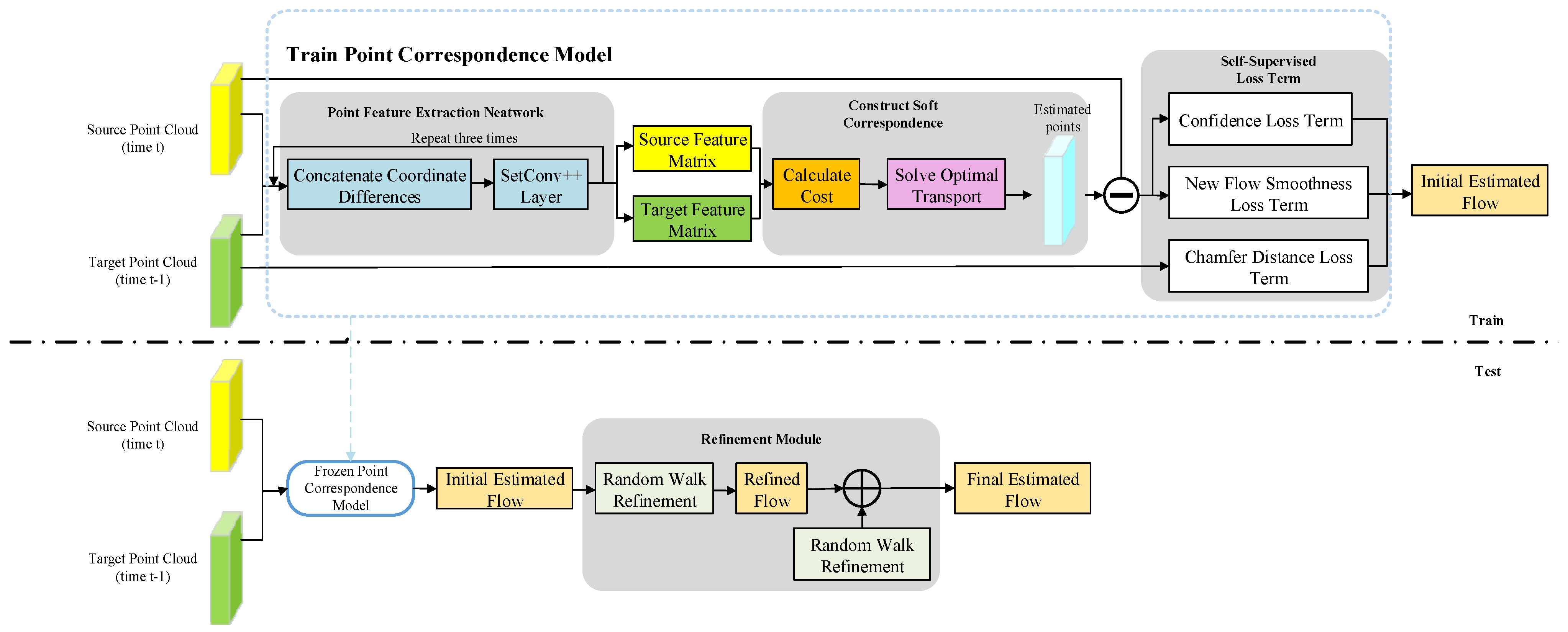
The initial step in the point correspondence model requires obtaining feature representations for every point within the source point cloud $P{C}_t$ and target point cloud $P{C}_{t+1}$. This foundational step enables the construction of soft correspondence points and the calculation of initial estimated flows. A deep network transforms the original 3D coordinates of each point into high-dimensional feature vectors. These vectors consequently capture the geometric information of the point clouds more effectively. The feature extraction network therefore processes $P{C}_t$ and $P{C}_{t+1}$ as input, outputting corresponding feature matrices $F_t\in R^{m\times d}$ and $F_{t+1}\in R^{m\times d}$, where $d$ denotes the dimensionality of the point features.

However, experiments using SCOOP [9] indicate that incorrect soft correspondences frequently occur when local regions contain similar structures. The root cause lies in the inaccurate feature representations of the points within these structures. This inaccuracy leads to insufficient differentiation between points residing in similar local areas. Consequently, during soft correspondence construction, points from nearby similar structures are often erroneously selected. To address this limitation, this paper proposes an improved point feature extraction network. This enhanced network specifically strengthens the model’s ability to learn local structural information within point clouds [34,35]. It mitigates the problem of ambiguous feature representation in geometrically similar regions.

The point feature extraction network in SCOOP [5] builds upon the PointNet++ [8] architecture. This network incorporates three SetConv layers. Each layer performs feature extraction while progressively expanding the dimensionality of the feature vectors. Specifically, the SetConv layer operates through three sequential stages: 2D convolution, instance normalization, and Leaky ReLU activation. Subsequently, it applies max pooling to aggregate information within local neighborhoods. This process ensures the final point features capture local geometric structure information effectively. However, this paper observes that the current network design underutilizes the feature information extracted during each processing stage. It relies solely on the highest-level features from the final stage for neighborhood feature aggregation. Consequently, the lower-level features generated in the first two stages remain insufficiently leveraged, despite their inherent utility for capturing nuanced local structural information within the point cloud.

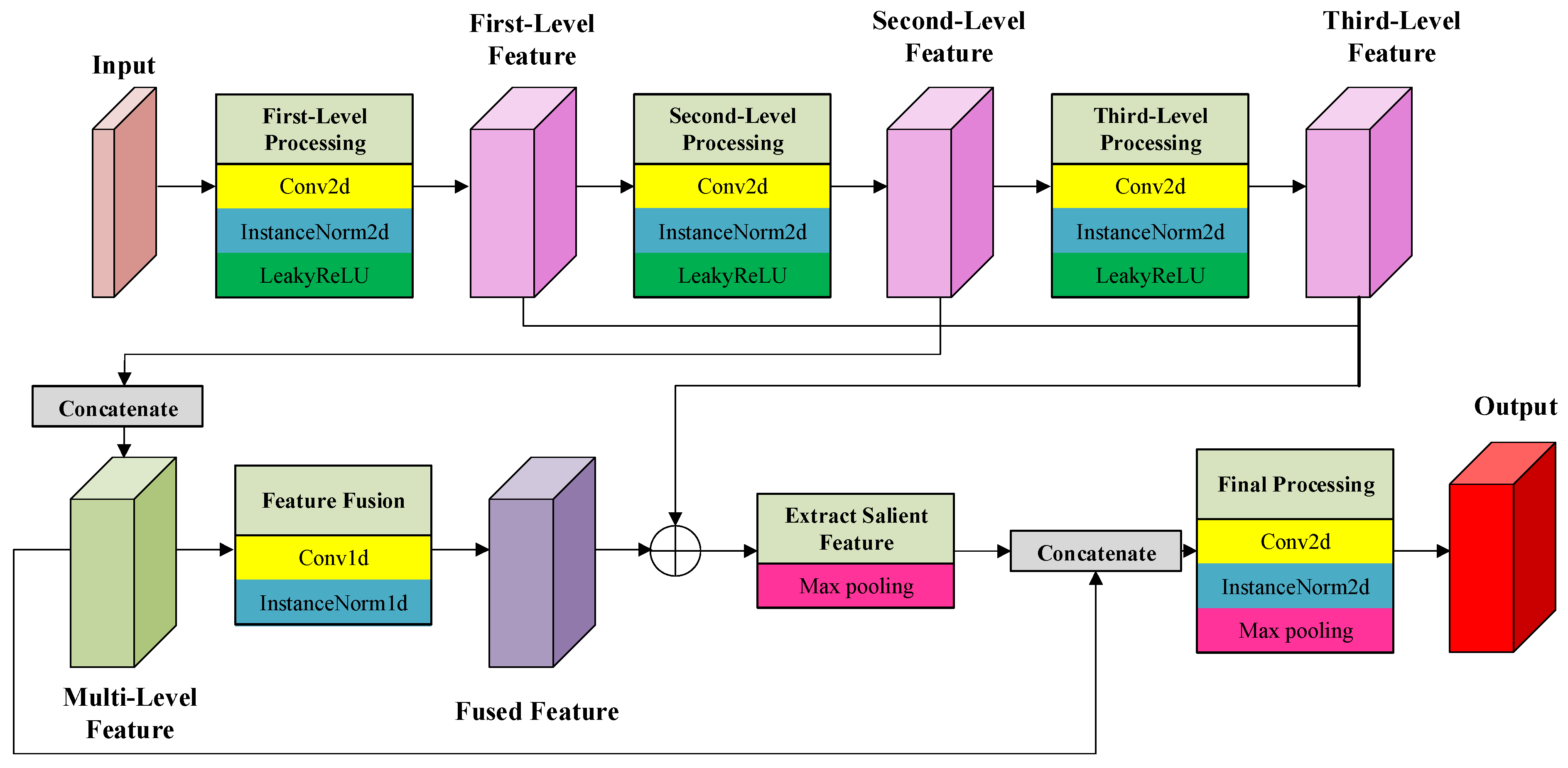
To address this limitation, the paper introduces enhancements to the SetConv layers. By more comprehensively leveraging features extracted at every stage, the network improves its capacity to represent local structures in unstructured, unordered point clouds. This improved variant is termed the SetConv++ layer. Figure 2 illustrates its structure.

Unlike the SetConv layer, the SetConv++ layer concatenates the three levels of features obtained after each processing stage along the feature dimension. This combined output is termed the concatenated multi-level feature. Subsequently, this concatenated feature undergoes convolution and instance normalization to reduce dimensionality, resulting in the fused multi-level feature. The fused multi-level feature then combines with the third-level feature through element-wise addition.

Following this operation, max pooling is applied within each local neighborhood to extract the most significant feature. This significant feature is then concatenated with the original concatenated multi-level feature along the feature dimension. The combined result is again reduced in dimensionality via convolution and instance normalization. Finally, max pooling is performed once more within the local neighborhood.

This improvement aims to better leverage local contextual information while emphasizing the most salient neighborhood features. Consequently, the network learns local point cloud structures more effectively. Consistent with SCOOP [5], the current feature vector concatenates with coordinate difference vectors between neighboring points and the center point. This concatenated output serves as input for the next SetConv++ layer. The purpose of this design is to integrate local spatial relationships, thereby enhancing local structure capture. The overall feature extraction network proposed in this paper comprises three SetConv++ layers, with k_n denoting the number of neighborhood points.

3.2. Construct Soft Correspondence

In this paper, we construct soft correspondences for each point in the source point cloud using the feature matrices $F_t$ and $F_{t+1}$. This process follows the method described in [5], which involves solving the optimal transport problem through Sinkhorn iterations with entropy regularization. This method solves the optimal transport problem through the Sinkhorn iteration controlled by the entropy regularization parameter $ϵ=0.03+{ϵ}^{learned}$ (where $ϵ$ learned is a learnable parameter). The setting of the final convergence value $ϵ$ ≈ 0.15 keeps the entropy of the corresponding matrix in a moderately softened state, balancing the matching accuracy and computational stability. Since the transport cost depends on inter-point similarity, we compute the cosine similarity matrix $S$ between features to represent the similarity between points in $P{C}_t$ and $P{C}_{t+1}$, as shown in Equation (1):

$$S_{ij}={\displaystyle \frac{F_t^i{F}_{t+1}^j}{{‖F_t^i‖}_2{‖F_{t+1}^i‖}_2}}$$

(1)

where $F_{\mathrm{t}}^{\mathrm{i}}$ represents the feature vector of the i-th point in $P{C}_t$, and $F_{t+1}^j$ represents the feature vector of the j-th point in $P{C}_{t+1}$.

By constructing and solving this optimal transport problem [36], we obtain the optimal transport matrix $T^{*}$. We then select the top $k_t$ points from $P{C}_t$ with the highest mass transferred to $P{C}_{t+1}$ based on $T^{*}$. The weights for these k_t points are calculated as shown in Equation (2):

$$w_{ij}={\displaystyle \frac{e^{T^{*}\left[i\right]\left[j\right]}}{{\sum }_{n\in inde{x}_t}{e}^{T^{*}\left[i\right]\left[n\right]}}}$$

(2)

where i, j, and n are the set of indices corresponding to these selected $k_t$ points in $P{C}_{t+1}$.

Using the calculated weights, the soft correspondence point of the i-th point in $P{C}_t$ at time $t+1$, denoted as ${\widetilde{ pc}}_{\mathrm{t}+1}^{\mathrm{i}}$, is obtained, as shown in Equation (3). The coordinate difference between the soft correspondence point ${\widetilde{pc}}_{\mathrm{t}+1}^{\mathrm{i}}$ and point $p{c}_t^i$ is used as the initial estimation of the scene flow at $p{c}_t^i$, denoted as $flo{w}_i\in R^3$.

Using these calculated weights, the soft correspondence point of the i-th point in $P{C}_t$ at time $t+1$, denoted as ${\widetilde{ pc}}_{t+1}^{\mathrm{i}}$, is determined. Its coordinate difference from point ${\widetilde{pc}}_{\mathrm{t}+1}^{\mathrm{i}}$ serves as the initial estimation of the scene flow at $p{c}_t^i$, denoted as $flo{w}_i\in R^3$:

$${\widetilde{pc}}_{\mathrm{t}+1}^{\mathrm{i}}={\sum }_{j\in inde{x}_t}{w}_{ij}p{c}_{t+1}^j$$

(3)

where $w_{ij}$ is the weight for point kt.

3.3. Self-Supervised Loss Term Design

Since ground truth data for point cloud scene flow is unavailable, effective training of the point model requires the introduction of self-supervised loss terms. SCOOP [5] proposes three such terms: a chamfer distance loss ($L_{dist}$), a confidence loss ($L_{conf}$), and a flow smoothness loss ($L_{smooth}$). This paper acknowledges that $L_{smooth}$ from [5] helps maintain local consistency of the estimated flow. However, it also propagates incorrect estimations. Therefore, building on $L_{smooth}$, this paper proposes a novel flow smoothness loss, $L_{smooth\_new}$. While preserving $L_{smooth\_new}$’s role in promoting local consistency, $L_{smooth\_new}$ also suppresses the spread of incorrect estimations. Consequently, this paper selects three self-supervised loss terms for training the point correspondence model: the chamfer distance loss and confidence loss from SCOOP [5], combined with the newly proposed flow smoothness loss term.

In this paper, the set of soft correspondences for the source point cloud $P{C}_t$ at time $t+1$ is denoted as ${\widetilde{PC}}_{t+1}$. The purpose of the chamfer distance loss term is to maximize the overlap between ${\widetilde{PC}}_{t+1}$ and the actual target point cloud $P{C}_{t+1}$. Compared to similar chamfer losses in prior works [6,37], SCOOP [5] introduces the concept of matching confidence, which indicates the reliability of the generated soft correspondences. This approach provides valuable insight for the subsequent improvement of the flow smoothness loss proposed in this work. The chamfer distance loss used here follows the same construction as described in SCOOP [5]. Specifically, the confidence $u_i$ for an estimated point ${\widetilde{pc}}_{\mathrm{t}+1}^{\mathrm{i}}$ is calculated using the cosine similarity matrix, as shown in Equation (4). Introducing this confidence into the chamfer distance loss term increases the supervision weight on high-confidence estimations, as shown in Equation (5).

$$u_i=max\left({\sum }_{j\in index}{w}_{ij}{S}_{ij},0\right)$$

(4)

$$L_{dist}={\displaystyle \frac{1}{m}}{\sum }_{x\in {\stackrel{△}{PC}}_{t+1}}{u}_x\underset{y\in P{C}_{t+1}}{min}||x-y{||}_2^2$$

(5)

where m is the number of three-dimensional points contained in the source point cloud PC_t and the target point cloud PC_t+1.

Additionally, building on [5], this paper constructs a confidence loss term to penalize low-confidence flow estimations, as shown in Equation (6).

$$L_{conf}={\displaystyle \frac{1}{m}}{\displaystyle \sum _{i=1}^m}1-u_i$$

(6)

The purpose of the flow smoothness loss term is to enhance the local consistency of the estimated point cloud scene flow. This ensures that neighboring points within $P{C}_t$ exhibit similar motion patterns. Consequently, the final surface of ${\widetilde{PC}}_{t+1}$ becomes as smooth as possible. In SCOOP [5], the flow smoothness loss term is constructed following this principle, as shown in Equation (7).

$$L_{\mathrm{smooth}}={\displaystyle \frac{1}{m}}{\displaystyle \frac{1}{k_s}}{\displaystyle \sum _{i=1}^m}\sum _{j\in inde{x}_s}\left|\left|flo{w}_i-flo{w}_j\right|\right|$$

(7)

where $k_s$ is the number of points taken from the neighborhood, and $inde{x}_s$ is the set of indices for these $k_s$ nearest neighbors.

While constructing the flow smoothness loss term as defined in Equation (7) enhances the local consistency of point cloud scene flow, this paper contends that it fails to account for the influence of erroneous estimations. Consequently, incorrect estimations propagate. In particular, the existing method assigns equal influence to every neighboring point on the center point’s flow estimate. This results in excessive negative impact from erroneous neighborhood estimations, further propagating errors. To address this limitation, this paper improves the original flow smoothness loss term $L_{smooth}$ from [5]. Inspired by SCOOP [5]’s integration of confidence into the chamfer distance loss, this work introduces confidence-aware weights for neighborhood influences. Specifically, high-confidence flow estimates exert greater influence on the center point, whereas low-confidence estimates have reduced impact. Similarly, the center point’s own confidence level determines its contribution to the total loss: higher confidence increases the contribution, and conversely, lower confidence decreases it. Therefore, consistency with reliable high-confidence flows is enhanced, while the detrimental influence of potentially erroneous low-confidence flows is mitigated. Consequently, the proposed loss term, denoted as $L_{smooth\_new}$, better maintains flow consistency and effectively prevents error propagation.

$$L_{\mathrm{smooth}\_\mathrm{new}}={\displaystyle \sum _{i=1}^m}{x}_i{\displaystyle \sum _{j=0}^{k_s-1}}{\widehat{x}}_j\left|\left|flo{w}_i-flo{w}_{inde{x}_s\left[j\right]}\right|\right|$$

(8)

where $x\in R^m$ is obtained by applying softmax to the global confidence vector $u\in R^m$ (associated with all elements). In contrast, $\widehat{x}\in k^s$ is obtained by applying softmax to $\widehat{u}\in k^s$, which is the local neighborhood confidence vector formed by selecting entries from $u$ corresponding to the indices in $inde{x}_s$.

In summary, the overall training loss consists of $L_{dist}$, $L_{conf}$, and $L_{smooth\_new}$, as shown in Equation (9).

$$L_{total}=\lambda L_{dist}+\mu L_{conf}+\nu L_{smooth\_new}$$

(9)

where$\lambda$, $\mu$, and $\nu$ are hyperparameters.

3.4. Design of the Refinement Module

Instead of directly refining the initial flow estimate with residual flow refinement as in SCOOP [5], this paper first employs a confidence-based random walk algorithm. While SCOOP’s refinement module aims to improve flow accuracy, experiments in [5] reveal that errors persist when target point clouds lack corresponding local regions from the source. These errors occur because selected soft correspondence points have no true counterparts, leading to fundamentally incorrect initial flow estimates in affected regions. Crucially, SCOOP’s residual refinement cannot correct such errors.

To address this limitation, the proposed random walk refinement adjusts high-confidence flow estimates further and reconstructs low-confidence estimates using neighboring high-confidence flows. This process enhances local flow consistency while specifically improving scenarios where missing corresponding regions in$P{C}_t$ (relative to $P{C}_{t+1}$) cause incorrect soft correspondences and erroneous flow estimations.

The random walk refinement module first constructs a graph on $P{C}_t$, denoted as $G(V,E)$, where the node set $V$ consists of all points in $P{C}_t$, and $E$ represents the edge set. Divide $V$ into two parts, with one part including all points where the confidence of the estimated flow is greater than or equal to threshold $\alpha$, denoted as $V_c$; the other part contains the remaining points where the confidence of the estimated flow is below threshold $\alpha$, denoted as $V_w$. The estimated flow at each point in $V_c$ is considered influential and only requires fine-tuning. In contrast, the estimated flow at each point in $V_w$ is deemed non-influential and needs to be reconstructed.

The points within set $V_c$ exhibit measurable influence. Consequently, adjusting their estimated flows necessitates only fine-tuning procedures. In contrast, points belonging to set $V_w$ lack significant influence. This characteristic necessitates the complete reconstruction of their flow estimates.

The distance influence matrix for the points within the graph $G(V,E)$ is defined as $W$. Specifically, all elements on the main diagonal of matrix $W$ are explicitly set to zero. Element $W_{ij}$ is calculated by Equation (10):

$$W_{ij}=e^{-{\displaystyle \frac{\left|\right|v^{\mathrm{i}}-v^{\mathrm{j}}|{|}_2}{\omega }}}$$

(10)

where $v^{\mathrm{i}}$ and $v^{\mathrm{j}}$ denote the spatial coordinates of the i-th and j-th nodes in $G(V,E)$, respectively. The hyperparameter ω controls the rate at which influence diminishes over distance. Consequently, higher values of $\omega$ generally result in weaker distance-based attenuation, while lower values yield a stronger decrease in influence as the distance between nodes increases. It should be noted that $\omega$ controls the decay rate of the neighborhood influence. When it approaches 0, the random walk degenerates into isolated point reconstruction, and low-confidence points only rely on themselves. When it approaches positive infinity, weights the of all points are equal, resulting in global over-smoothing and destroying the motion boundary.

The subsequent step involves computing the transition probability matrix. Within this framework, the estimated flow confidence at each point contributes to the calculation. Specifically, points exhibiting confidence values exceeding a predefined threshold $\omega$ are retained. Conversely, points with confidence values below $\omega$ are set to zero. Points retained under this criterion are designated as $valid$. Finally, normalization is applied to the valid points. This normalized result defines the transition probability matrix, denoted as $M$, as shown in Equation (11).

$$M_{ij}={\displaystyle \frac{vali{d}_j{W}_{ij}}{{\sum }_{j=i}^m{W}_{ij}}}$$

(11)

The fine-tuning and reconstruction parts are performed in the same manner as in [32]. The estimated flow at each point in $V_c$ after $i$ iterations of fine-tuning is denoted as $Flo{w}^{\left(i\right)}$, as shown in Equation (12).

$$Flo{w}^{\left(i\right)}=\tau M\times Flo{w}^{i-1}+(1-\tau )Flo{w}^{\left(0\right)}$$

(12)

where $Flo{w}^{\left(0\right)}$ is the initial estimated flow, and $\tau \in \left[\mathrm{0,1}\right]$ is the parameter used to adjust the strength of the random walk adjustment.

$Flo{w}^{\left(i\right)}$ gradually converges as the number of iterations increases. When $i=\infty$, the estimated flow after infinite iterations can be computed, denoted as, as shown in Equation (13).

$$Flo{w}^{\left(\infty \right)}=(1-\tau ){\left(I−\tau M^{-1}\right)}^{-1}Flo{w}^{\left(0\right)}$$

(13)

Reconstruct the estimated flow at each point in $V$ based on $Flo{w}^{\left(\infty \right)}$, denoted as $Flo{w}_{alter}$. The reconstruction process is shown in Equation (14).

$$Flo{w}_{alter}=M\times Flo{w}^{\left(\infty \right)}$$

(14)

By using the fine-tuned estimated flow $Flo{w}^{\left(\infty \right)}$ and the reconstructed estimated flow $Flo{w}_{alter}$, the complete estimated flow after random walk refinement can be obtained. Unlike in [32], where all flows are directly replaced based on reliability, this paper introduces two confidence thresholds (α and β), with β > α. Points are divided into three parts based on their flow estimation confidence.

Points with confidence in the estimated flow within the interval $\left[0,\alpha \right]$ are categorized as the first part, and their corresponding indices are denoted as$P_1$. For points in this part, the estimated flow is directly replaced with the corresponding part from $Flo{w}_{alter}$. Points with confidence in the estimated flow within the interval $\left[\alpha ,\beta \right]$ are categorized as the second part, and their corresponding indices are denoted as$P_2$. For points in the second part, the estimated flow is replaced by a mixture of the corresponding parts from $Flo{w}^{\left(\infty \right)}$ and $Flo{w}_{alter}$, according to a certain ratio. The mixing ratio should be such that the lower the original estimated flow’s confidence, the higher the proportion of $Flo{w}_{alter}$; conversely, the higher the confidence, the lower the proportion of $Flo{w}_{alter}$. Points with confidence in the flow estimate within the interval $\left[\beta ,1\right]$ are categorized as the third part, and their corresponding indices are denoted as $P_3$. For points in the third part, the estimated flow is directly replaced with the corresponding part from $Flo{w}^{\left(\infty \right)}$.

The final result is denoted as $Flo{w}_{r\mathrm{w}}$, as shown in Equation (15).

$$\begin{array}{c}Flo{w}_{rw}=P_3·Flo{w}^{\left(\infty \right)}+P_1·Flo{w}_{alter}\\ +P_2·valid·Flo{w}^{\left(\infty \right)}\\ +P_2·(1-valid)Flo{w}_{alter}\end{array}$$

(15)

The selection of confidence thresholds α and β (where β > α) is critical for balancing the contributions of $Flo{w}^{\left(\infty \right)}$ and reconstructed $Flo{w}_{alter}$ flows in the final output $Flo{w}_{r\mathrm{w}}$. To address potential concerns regarding their sensitivity to different data distributions and environmental conditions, we conducted extensive ablation studies across diverse datasets. As comprehensively demonstrated in Section 4.3 (Ablation Study), the optimal values of α and β identified on our primary validation split exhibit remarkable robustness. These optimal thresholds consistently delivered high performance not only across different splits of the same dataset but also when applied to datasets featuring significantly different environmental characteristics and point densities. While the optimal values are derived empirically, their robustness across varying conditions suggests they capture a fundamental balance between flow confidence and the need for neighbor-based reconstruction applicable to general dynamic point cloud scenes. After processing through the random walk refinement, the residual flow refinement used in SCOOP [5] is then applied. Residual flow refinement allows the estimated target point cloud ${\widetilde{PC}}_{t+1}$, formed by the estimated scene flow, to better preserve the geometric structure of the source point cloud $P{C}_t$. It also brings ${\widetilde{PC}}_{t+1}$ closer to the surface of the target point cloud $P{C}_{t+1}$. The implementation involves adding a residual flow refinement component, denoted as $Flo{w}_r\in R^{m\times 3}$, on top of $Flo{w}_{r\mathrm{w}}$ for fine-tuning. Optimization of $Flo{w}_r$ is performed by supervising it with Equations (7) and (9), which serve as the chamfer distance loss term and flow smoothness loss term, respectively. This ensures the estimated result aligns more closely with the target point cloud. The final estimated point cloud scene flow is denoted as $Flo{w}_{final}\in R^{m\times 3}$, as shown in Equation (16).

$$Flo{w}_{final}=Flo{w}_{rw}+Flo{w}_r$$

(16)

4. Experimental Results and Analysis

The experiments in this paper were conducted on the Kaggle platform using a P100 GPU. Training and testing were performed in an environment with Ubuntu 22.04, Python 3.10.12, CUDA 11.8, cuDNN 8.9, and PyTorch 3.10.12.

4.1. Selection of Datasets

This paper conducts experiments using the KITTI dataset [18], a real-world autonomous driving dataset with ground-truth scene flow annotations. Raw data from KITTI Scene Flow does not provide point clouds in the required format; point clouds are extracted from the training set’s 150 samples as in [18]. We removed ground points to reduce computational cost and retained occluded points to enhance prediction robustness. As the largest-scale rigid region, ground points are prone to being over-emphasized by the model in terms of point correspondence. In the optimal transport problem, the similarity matrix of ground points will dominate the transport solution, resulting in a large amount of computing resources being used for the correspondence of ground points with high confidence but low information content, while the matching of dynamic objects is diluted. Although retaining ground points can improve theoretical robustness, the graph construction of random walk relies on neighborhood search. The addition of ground points increases the graph scale and slows down the convergence. Therefore, the removal of ground points in this paper is a targeted design based on efficiency and dynamic target estimation. Following the partitioning method established by Mittal et al. [6], KITTI is divided into two subsets for the experiments: KITTIv, which contains 100 point cloud samples, and KITTIt, which contains 50 point cloud samples. KITTIv serves as the training set, while KITTIt serves as the test set. To enable comparison with fully supervised point cloud scene flow estimation methods, which typically require large volumes of ground truth data for training, we additionally utilize the FT3D dataset [18]. This dataset provides 18,000 training samples, where each sample includes a pair of adjacent point clouds along with their corresponding ground truth scene flow.

4.2. Evaluation Metrics

This paper adopts the standard evaluation metrics commonly used in previous work on point cloud scene flow estimation. These include end-to-end error EPE (m), strict accuracy AS (%), relaxed accuracy AR (%), and outlier probability Out (%). In addition, this paper introduces the newly proposed angular error AE to more effectively evaluate the directional accuracy of the estimated point cloud scene flow. The construction of AE is shown in Equation (17).

$$AE=1-{\displaystyle \frac{1}{m}}{\sum }_{i=1}^m{\displaystyle \frac{flo{w}_{final}^i·flo{w}_t^i}{‖flo{w}_{final}^i‖·‖flo{w}_t^i‖·}}$$

(17)

4.3. Ablation Study

First, to demonstrate the effectiveness of the proposed SetConv++ layer, the new flow smoothness loss term, and the random walk refinement module, this section conducts a series of ablation experiments. Ablation studies decompose intelligent systems to quantify component-level contributions, aligning with modularity (isolating functional units), interpretability (linking design to metrics), and efficiency-accuracy trade-off. To validate our proposed SetConv++, novel loss, and random walk refinement, we design eight scenarios (

Table 1. Ablation Experiment Results.

Set	EPE (m)	AS (%)	AR (%)	Out (%)	AE
(a)	0.0411	92.68	96.10	15.78	0.0777
(b)	0.0395	92.99	96.70	15.07	0.0772
(c)	0.0391	93.99	96.42	15.26	0.0783
(d)	0.0381	94.24	97.10	14.61	0.0776
(e)	0.0381	93.71	96.60	14.87	0.0785
(f)	0.0375	93.80	96.79	14.88	0.0779
(g)	0.0357	95.03	97.20	14.23	0.0768
(h)	0.0355	95.11	97.37	14.28	0.0762

) by incrementally modifying components against a baseline.

The experimental setup includes the following eight different scenarios: (a) Use the original network structure called SetConv layer, the original flow smoothness loss term, and the original refinement module; (b) Use the original network structure called SetConv layer, the original flow smoothness loss term, and the random walk-based refinement module; (c) Use the original network structure called SetConv layer, the new flow smoothness loss term, and the original refinement module; (d) Use the original network structure called SetConv layer, the new flow smoothness loss term, and the random walk-based refinement module; (e) Use the proposed network structure called SetConv++ layer, the original flow smoothness loss term, and the original refinement module; (f) Use the proposed network structure called SetConv++ layer, the original flow smoothness loss term, and the random walk-based refinement module; (g) Use the proposed network structure called SetConv++ layer, the new flow smoothness loss term, and the original refinement module; (h) Use the proposed network structure called SetConv++ layer, the new flow smoothness loss term, and the random walk-based refinement module.

The results of the ablation experiment are shown in Table 1. The experimental results demonstrate that the proposed SetConv++ layer, the novel flow smoothness loss term, and the random walk refinement module effectively enhance the performance of point cloud scene flow estimation. The notable performance gain from scenario (f) to scenario (g) shows a significant EPE reduction of 0.0018, from 0.0375 to 0.0357. This improvement primarily stems from the synergistic interaction between the SetConv++ layer and the new flow smoothing loss term. SetConv++ enhances initial feature extraction, leading to more accurate base flow estimation. Simultaneously, the new loss term explicitly enforces spatial coherence. Together, they jointly optimize the core estimation process to reduce global errors. In contrast, the refinement module, as used in scenario (f), operates afterwards to adjust local details. This yields smaller incremental gains. The synergy demonstrates that architectural innovations like SetConv++ and novel loss formulations provide more fundamental improvements than post-processing modules alone.

Second, a series of experiments were conducted to validate the setting of the number of nearest neighbors. In these experiments, different values were set for the nearest neighbor parameters $k_n$, $k_t$ and $k_s$. $k_n$ represents the number of nearest neighbors within the local neighborhood during feature extraction, $k_t$ represents the number of candidate points selected when constructing soft correspondences, and $k_s$ represents the number of neighboring points that support the estimated flow of the center point in the flow smoothness loss term. The results are shown in

Table 2. Neighbor Number Parameter Setting Experiment Results.

Set		EPE (m)	AS (%)	AR (%)	Out (%)	AE
(a.1)	kn = 8	0.0424	92.56	95.17	16.31	0.0794
(a.2)	kn = 16	0.0388	93.28	96.25	15.23	0.0782
(a.3)	kn = 32	0.0355	95.11	97.37	14.28	0.0762
(b.1)	kt = 16	0.0362	94.99	97.26	14.24	0.0763
(b.2)	kt = 32	0.0361	94.74	97.33	14.23	0.0763
(b.3)	kt = 64	0.0355	95.11	97.37	14.28	0.0762
(c.1)	ks = 16	0.0434	91.03	95.28	17.37	0.0786
(c.2)	ks = 32	0.0355	95.11	97.37	14.28	0.0762
(c.3)	ks = 64	0.0372	94.44	97.10	14.54	0.0777

. The experimental results show that setting the nearest neighbor parameters $k_n$, $k_t$ and $k_s$ to 32, 64 and 32, respectively, achieves the best prediction performance.

Third, a series of experiments were conducted to determine the specific values of the two thresholds used in the random walk-based refinement module. By observing the impact of different threshold settings on the final prediction results, the most suitable values are selected. The experimental results are shown in

Table 3. Threshold Parameter Setting Experiment Results.

	Set	EPE (m)	AS (%)	AR (%)	Out (%)	AE
(a.1)	α = 0.0, β = 1.0	0.0356	95.09	97.32	14.29	0.0761
(a.2)	α = 0.1, β = 1.0	0.0356	95.09	97.32	14.29	0.0761
(a.3)	α = 0.2, β = 1.0	0.0356	95.09	97.32	14.29	0.0762
(a.4)	α = 0.3, β = 1.0	0.0357	95.09	97.32	14.29	0.0761
(b.1)	α = 0.0, β = 0.9	0.0356	95.11	97.32	14.31	0.0761
(b.2)	α = 0.1, β = 0.9	0.0356	95.11	97.32	14.31	0.0761
(b.3)	α = 0.2, β = 0.9	0.0356	95.11	97.32	14.30	0.0761
(b.4)	α = 0.3, β = 0.9	0.0357	95.11	97.18	14.30	0.0761
(c.1)	α = 0.0, β = 0.8	0.0355	95.11	97.37	14.28	0.0762
(c.2)	α = 0.1, β = 0.8	0.0355	95.11	97.37	14.28	0.0762
(c.3)	α = 0.2, β = 0.8	0.0355	95.11	97.37	14.28	0.0762
(c.4)	α = 0.3, β = 0.8	0.0356	95.11	97.37	14.28	0.0762
(d.1)	α = 0.0, β = 0.7	0.0356	95.09	97.32	14.30	0.0762
(d.2)	α = 0.1, β = 0.7	0.0356	95.09	97.32	14.30	0.0762
(d.3)	α = 0.2, β = 0.7	0.0356	95.09	97.32	14.30	0.0762
(d.4)	α = 0.3, β = 0.7	0.0357	95.09	97.32	14.30	0.0762

. The result shows that setting the value of $\beta$ to 0.8 achieves the best overall prediction performance. However, the value of $\alpha$ does not significantly impact overall prediction performance. The reason is that there are very few estimated flows with confidence in the low range $\left[0,\alpha \right]$. Therefore, reconstructing these low-confidence estimates has a minimal impact on overall performance. It was also found that setting the value of $\alpha$ to 0.3 slightly decreases prediction performance. This reason might be that the accuracy of adjusted estimates in the confidence range [0.2, 0.3] is higher than that of reconstructed estimations. Therefore, the value of $\alpha$ is set to 0.2 in this paper.

The physical meanings of $\alpha$ = 0.2 and $\beta$ = 0.8 not only stem from the geometric reliability of point classification but are also reflected in how they model the dynamic behavior of point clouds through the scene flow confidence under physical constraints. In the ablation study in Table 3, $\alpha$ = 0.2 corresponds to the upper tolerance limit for environmental noise. In dynamic scenes, sensor noise, partial occlusion, or motion blur usually create uncertain regions in the point cloud. Setting $\alpha$ too low will miss key error points, leading to the divergence of flow estimation; while setting it too high will over-label error points, increasing the reconstruction burden. $\beta$ = 0.8 reflects the probability threshold of geometric stability. In rigid body motion or static regions, the consistency of point displacement and the degree of feature matching are usually too high. A $\beta$ value lower than 0.7 will include too many medium-confidence points, diluting the reliability of anchor points; a value higher than 0.9 will result in too few anchor points, failing to effectively cover the scene. Therefore, this threshold selection physically optimizes the efficiency of the random walk refinement module. Moreover, $\alpha$ and $\beta$ divide the point cloud into low-confidence areas, verification areas, and reference sources through hierarchical confidence management. This adapts to common physical interferences under real-world conditions and improves robustness.

Fourth, experiments were conducted to show that the proposed method can be trained effectively with a small number of samples, without relying on a large amount of point cloud data. Training was conducted using the KITTI_r dataset with 6068 sample pairs and the KITTI_v dataset with 100 sample pairs. Performance was then evaluated on the KITTI_t dataset. The result of the experiment is shown in

Table 4. Training Sample Quantity Comparison Experiment Results.

Train Data	EPE (m)	AS (%)	AR (%)	Out (%)	AE
KITTIv (100)	0.0355	95.11	97.37	14.28	0.0762
KITTIr (6068)	0.0426	92.51	95.90	15.60	0.0784

. The result proves that only 100 sample pairs are sufficient to support the training of the proposed model.

Fifth, to evaluate the robustness of the proposed method, corresponding experiments are conducted. Gaussian noise with standard deviations $\sigma$ of 0.01 and 0.02 is added separately to each target point cloud. Based on this, experiments are carried out to compare the scene flow estimation performance of the proposed method and the baseline method SCOOP under noisy conditions. As shown in

Table 5. Noise Experiment Results.

Intensity	Method	EPE (m)	AS (%)	AR (%)	Out (%)	AE
σ = 0.01	SCOOP [5]	0.0419	92.33	96.03	16.25	0.0777
	Ours	0.0365	94.75	97.24	14.72	0.0763
σ = 0.02	SCOOP [5]	0.0432	91.63	95.74	16.90	0.0779
	Ours	0.0380	93.44	97.06	15.35	0.0765

, the results demonstrate that the proposed method outperforms the baseline under different levels of noise.

Meanwhile, we can directly observe that the method proposed in this paper maintains higher accuracy than SCOOP under Gaussian noise. The theoretical reason lies in that our method is specifically designed at key steps, effectively suppressing noise interference. Specifically: First, in the point-to-point correspondence model, we extract richer and more robust contextual information by fusing multi-layer features, making the point feature representation less sensitive to noise perturbations. Thus, when constructing the transport cost and solving the optimal transport problem, we can more accurately establish the correspondence between point clouds and obtain a more noise-robust initial flow estimate. Second, the random walk algorithm introduced in the flow refinement module can effectively identify and reconstruct the low-confidence initial flow regions caused by noise and improve local consistency through fine-tuning, which significantly enhances the model’s adaptability to noisy points or local distortions. In addition, the flow smoothing loss term based on confidence weighting proposed by us avoids the problem of error estimation diffusion caused by uniform smoothing and suppresses the propagation of noise errors, especially in high-noise regions (usually corresponding to low confidence). These improvements in design work together, enabling our method to estimate the scene flow more accurately in a noisy environment, thus outperforming SCOOP in terms of accuracy metrics.

4.4. Comparison and Analysis of Experiments

The model trained on the KITTIv dataset is used to test and evaluate the proposed method on the KITTIt dataset. Following [5], the hyperparameters in the self-supervised loss functions are set as $\lambda =1$, $\mu =0.1$, and $\nu =10$.

The comparison of experimental results between the proposed method and the original method [5] on the KITTIt dataset are shown in Figure 3 and Figure 4. In the figures, the dark blue points represent the source point cloud, the light blue points represent the target point cloud, the green points represent the point cloud obtained by processing the source point cloud with the ground truth point cloud scene flow, and the red points represent the point cloud obtained by processing the source point cloud with the estimated point cloud scene flow.

Figure 3 compares the results across three scenes where the corresponding regions in the source point cloud are not captured by the target point cloud. Figure 3 shows the comparative experimental results across six scenes where the method in [5] produced significant errors in local regions with similar adjacent structures. In contrast, the method proposed in this paper achieves superior performance in both the scenarios illustrated in Figure 3 and Figure 4.

In this section, the method proposed in this paper is compared with several recent self-supervised methods on the KITTI_t dataset. These methods are evaluated on the KITTI_t dataset, and the comparative result is shown in

Table 6. Comparison Results of Self-Supervised Methods.

Method	Train Data	EPE (m)	AS (%)	AR (%)	Out (%)	AE
SPF [32]	KITTIt (6068)	0.1008	37.46	71.54	49.28	0.3991
RigidFlow [38]	KITTIt (6068)	0.1026	44.77		44.63	0.3704
SPFlowNet [37]	KITTIt (6068)	0.0794	68.73		31.68	0.3400
SSFlowNet [33]	KITTIv (100)	0.0390	88.30	72.43	22.60	-
SCOOP [5]	KITTIv (100)	0.0411	92.68	84.42	15.78	0.0777
Ours	KITTIv (100)	0.0355	95.11	97.37	14.28	0.0762

. The numbers in brackets in the table indicate the number of samples included in the training data. The results show that our method achieves the best performance, even when trained on the smallest amount of point cloud data.

In addition to comparing the proposed point cloud scene flow estimation method with other self-supervised methods, we also conducted comparison experiments with recent fully supervised methods. Each method is trained on the FT3Do dataset and evaluated on the KITTI_o dataset. The results of the comparison experiments are shown in

Table 7. Comparison Results with Supervised Methods.

Method	Train Data	EPE (m)	AS (%)	AR (%)	Out (%)	AE
FlowNet3D [18]	FT3Do	0.1748	9.97	42.09	77.07	0.5790
FLOT [21]	FT3Do	0.1127	40.23	70.70	49.67	0.0817
OGSFNet [39]	FT3Do	0.0781	70.07	86.55	33.79	0.0782
3DFlow [40]	FT3Do	0.0736	81.30	88.85	26.43	0.1270
DBINR [41]	FT3Do	0.0463	84.44	94.60	11.43	-
NRP [23]	FT3Do	0.0262	92.05	97.25	13.93	-
Ours	FT3Do	0.0399	92.45	96.75	15.10	0.0763

. The results of the comparison experiments show that the self-supervised method proposed in this paper performs slightly worse overall than the newly proposed fully supervised method NRP [23] in 2025. This demonstrates that the method in this paper can achieve excellent point cloud scene flow estimation performance without requiring ground truth data for supervision.

However, it should be noted that the performance improvement of supervised models such as NRP in processing extremely sparse point clouds largely depends on a large amount of prior knowledge from dense annotations. This poses significant challenges in real-world scenarios: the annotation cost is extremely high, and the problem of annotation noise is particularly prominent in sparse point clouds (such as long-distance target perception in autonomous driving). In contrast, our self-supervised method enhances the feature discrimination of sparse points by designing a feature extraction network and introduces an asymmetric receptive field mechanism to assign higher weights to isolated points, effectively improving the robustness in sparse environments. Similarly, in complex occlusion scenarios caused by multi-target interactions on urban roads, occlusion can disrupt motion consistency, and the NRP model that relies on complete annotations is prone to failure at occlusion boundaries. Our method, on the other hand, utilizes the dynamic weight adjustment mechanism of the flow smoothness loss term to effectively predict occlusion areas and reduce the errors they bring. Therefore, in the face of annotation scarcity and extreme conditions (such as high sparsity and strong occlusion) encountered commonly in real-world scenarios, our method demonstrates its unique advantages.

5. Conclusions

We propose a new self-supervised method for point cloud scene flow estimation. Our approach incorporates a SetConv++ layer that learns point feature representations more effectively, enabling the construction of more accurate soft correspondences. Furthermore, the flow smoothness loss term is employed during training for self-supervision, keeping the initial estimated flow smooth while mitigating erroneous expansions. Additionally, a refinement module based on the random walk algorithm adjusts the initial flow, effectively correcting errors from previous methods. The practical significance of this work is underscored by its ability to address real-world challenges: By significantly reducing dependence on expensive, manually labeled point cloud data, our method substantially improves its feasibility in scenarios like industrial inspection and warehouse robotics, where large-scale labeling is impractical and costly. Moreover, the effective suppression of error propagation within the estimated flow directly contributes to enhanced accuracy in path-planning systems for autonomous driving, a domain where precision is critical for safety and efficiency. The experimental results on the challenging KITTI Scene Flow dataset demonstrate that our method yields excellent performance. It requires only unlabeled point cloud data for training and outperforms existing self-supervised and supervised methods across various metrics, achieving state-of-the-art results. Crucially, ablation studies reveal marked improvements in key metrics: EPE decreases by 13.6% to 0.0355 m, AS increases to 95.11%, AR to 97.37%, and AE reduces to 0.0762 compared to the baseline. Although the SetConv++ layer in this paper increases the channel dimension by concatenating multi-level features, its main structure remains a cascaded lightweight SetConv layer, maintaining computational isomorphism with the original SetConv of SCOOP. The theoretical computational complexity increases due to feature concatenation and hierarchical expansion, but this overhead is greatly compressed through sparse voxelization technology. Additionally, the complexity of the neighborhood search iterative weighted average process in the random walk refinement module is accounted for in the design. Consequently, the total latency is estimated to meet real-time requirements for autonomous driving. However, these optimizations do not eliminate all challenges: despite these strengths, our approach has certain limitations. Performance may degrade in extremely sparse scenes due to reduced local context, and the random-walk refinement introduces extra inference time overhead compared to regression baselines. Looking ahead, future work will explore optimizing the inference efficiency of our framework for real-time deployment in autonomous driving systems, addressing potential constraints posed by platforms like GPUs.