A Network-Cascade Framework for Short-Run Production Failure Under Maritime-Energy Chokepoint Disruption

Abstract

Abrupt maritime-energy disruption can generate system-wide production losses before firms and policymakers can adjust. Existing assessments usually emphasize direct exposure or long-run equilibrium responses, which makes them less suitable for short-run risk assessment in energy-dependent production systems. We develop a threshold-cascade framework that combines dual-track dependence topology, edge-level inventories, smooth operability bands, and a separate price-validation step to identify the blockade intensity at which a localized chokepoint shock becomes systemic production loss. The framework is evaluated against the March 2021 Suez blockage and the 2022 Russia–Ukraine producer-price episode, and then applied to a 2026 Strait of Hormuz stress scenario using the Organisation for Economic Co-operation and Development (OECD) Inter-Country Input-Output (ICIO) tables, 2025 edition, with the 2022 benchmark year. Under the baseline 150-day horizon, terminal loss first reaches 50% at about 32% blockade intensity, with a broader calibrated threshold band of 32–46%. Losses spread beyond the point of origin and become concentrated in East and Southeast Asian manufacturing supply chains and in downstream consumer markets after inventories at connected hubs are depleted. Policy experiments show that single-channel interventions shift the threshold only modestly, whereas an integrated package that relaxes logistics, inventories, and upstream scarcity moves the threshold to about 46% in this calibration. The analysis targets the weeks-to-months interval before substitution, contract renegotiation, and broader market adjustments dominate. Within that interval, the model identifies when buffers fail, how production losses spread, and which intervention packages delay systemic disruption.

1. Introduction

Modern cross-border production systems depend heavily on a small number of maritime energy chokepoints, and the Strait of Hormuz is one of the most important [1,2,3,4,5]. Intermediate and specialized inputs often cross borders several times before final assembly. In such a tightly connected system, a local interruption at a chokepoint can quickly spread beyond the disrupted route. Shipping disruptions and energy shortages move along established input links, often faster than markets can reallocate them. During the first weeks of a crisis, the key issue is often the point at which inventories at key nodes are exhausted. Related evidence also comes from oil and gas studies: geopolitical risk, inventory compression, and transport friction often rise together, increasing both shortage risk and price volatility [6,7,8,9,10]. Once the buffer at a critical node is breached and no short-run physical substitute is available, the production network can move from stress to forced curtailment. The central task is therefore to identify when a local shock exhausts system buffers and becomes a network-wide production disruption.

Most standard tools for quantifying shocks of this kind still rely on static input-output accounting or computable general equilibrium models [11,12,13,14]. They are useful when the task is to measure steady-state loss or longer-run structural adjustment. They are less suitable for abrupt, short-run interruption. CGE models absorb shocks through smooth price adjustment and substitution. Static proportional-loss models also presuppose frictionless transmission. These approaches often omit the physical rigidity of actual supply chains. Firms cannot replace a missing critical input immediately. Even when prices move, cross-border producer-price and inflation pass-through still travel through existing input linkages and do not remove material scarcity by themselves [15,16,17]. The relevant time scale is important because firms first draw down inventories before production is curtailed [18,19,20,21]. During that interval, aggregate losses can remain limited even when upstream scarcity is building. Once inventories are exhausted and no short-run substitute is feasible, production can be interrupted in a distinctly nonlinear way [22,23,24,25,26,27,28]. Those forced stoppages then move downstream through a tightly coupled input-output topology and can convert a local shortage into a sharp aggregate loss. When the policy question shifts from long-run average damage to the short-run threshold of system breakage, models built around smooth adjustment become less suitable.

Capturing the cascade from buffer depletion to system breakage requires one framework that keeps network topology, transmission delay, and logistics boundaries in the same analytical space. At present, those elements still sit in three adjacent but only partially connected literatures. Production-network studies establish the topological basis of shock amplification. They show that output disturbances at individual nodes can be magnified through asymmetric input dependence [23,29,30,31,32,33,34] and transmitted across regions through supplier-customer linkages [24,25,26,35,36,37]. More general work on complex networks and cascade failure provides the language of threshold breakage [38,39,40,41,42]. Recent studies in complex-network dynamics have further examined collapse transitions under constrained detection, higher-order interaction effects, and data-driven prediction of information cascades [43,44,45]. Yet much of that literature works with steady networks or annual data and strips out inventory drawdown and physical delay. Dynamic disaster and inoperability models move directly to the time dimension and identify the role of stock buffers in absorbing early shock [12,18,19,20,21,46,47,48,49,50]. Their applications, however, are usually confined to national infrastructure disruption or regional natural hazards rather than a global maritime-energy network. Maritime and logistics studies recover the physical boundaries with much greater precision. They quantify rerouting costs, throughput loss, and time penalties after chokepoint disruption [1,2,4,5,51,52,53]. What remains much less explicit there is how those frictions cross industrial boundaries and become forced production cuts far from the port or sea lane itself. Each piece of the literature contributes something essential. They do not yet converge into one operational short-run threshold framework.

Recent work has brought these strands closer, especially in settings where inventories, transport delay, price pass-through, and global bottlenecks coexist. Studies on post-pandemic supply-chain adjustment have begun to estimate the combined effects of shutdowns, shortages, shipping delay, and inventory behavior [27,28,49,54]. Work on prices shows that international input linkages, shipping costs, and global supply pressure pass systematically into producer prices and inflation [15,16,17]. Research on maritime chokepoints and energy security has also progressed from port criticality to systemic chokepoint exposure, Suez-disruption loss, and geopolitical oil-price risk [1,2,4,5,6,9,53]. Even so, most studies still choose one main layer of analysis. Some emphasize network amplification, others inventory buffering, transport disruption, or price variation. Related epidemic-network studies also show that heterogeneous control, adaptive behavior, and multilayer information-epidemic coupling can materially shift thresholds and control outcomes [55,56,57]. Much less common is a tractable framework that makes these mechanisms work together to identify a short-run failure threshold.

Against that background, this study develops a threshold-cascade framework for diagnosing near-term production failure under abrupt maritime-energy disruption. Using the Organisation for Economic Co-operation and Development (OECD) Inter-Country Input-Output (ICIO) tables, 2025 edition, and extracting the 2022 benchmark year [58,59], the model preserves the observed scale of country-sector output while simulating shortage propagation in discrete time across an interconnected production system. A local disruption is not transmitted to the whole network at once. It moves only after logistics delay is traversed and node-level inventories are exhausted. The quantity side is carried by three linked components: dual-track dependence topology, edge-level inventories, and smooth operability bands. Together they support short-run risk assessment and resilience planning. In parallel, the framework includes a separate price-validation layer. Because the setting is explicitly nonequilibrium in the short run, that price path is one-directional. It records the implied price pulse but does not feed back to reallocate quantities. Its role is limited to external validation. It provides an observed benchmark for checking whether the timing and broad scale of price escalation are consistent with historical data.

To keep the observed event background separate from scenario construction, the 2026 Strait of Hormuz episode is used as an empirical scenario constraint, not an ex post reconstruction. Under the dated U.S. Energy Information Administration (EIA) and PortWatch snapshots used here [60,61], the military escalation after 28 February 2026 corresponds to a near-closure shock. PortWatch daily tanker data imply that average tanker deadweight tonnage passing through the strait fell by about 80.2% between 28 February and 5 March relative to the week before [61]. Over the same quarter, the EIA reported Brent rising from about $61 per barrel at the start of 2026 to about $118 per barrel by the end of the first quarter [60]. That dated evidence serves two purposes. It bounds the shock scale with observational data, and it clarifies the policy question: under what conditions do buffering mechanisms fail, where are losses concentrated, and which intervention packages delay systemic disruption most effectively? The framework does not model contract-level shipments or long-run feedback during that episode. It is built instead to measure the short-run output floor of the global network under explicit physical constraints. Before turning to the Hormuz simulations, the paper therefore uses the March 2021 Suez blockage and the 2022 Russia–Ukraine shock as empirical checks on the logistics-delay channel and the price-validation layer.

2. Materials and Methods

This study treats maritime-energy disruption as a dynamic cascade process on a country-sector production network. Over a horizon of weeks to months, firms usually cannot reorganize sourcing fast enough to keep pace with the spread of shortage. During that interval, physical constraints dominate price clearing. The framework is designed to recover the quantity-side output floor of the system under explicit assumptions about inventory depletion, technical rigidity, and sectoral tolerance.

The framework relies on four components. Dual-track dependence topology isolates hard bottlenecks inside a dense trade matrix. Smooth operability bands describe the gradual decay that firms experience before full stoppage. Edge-level inventories determine the time lag between measured dependence and physical interruption. The separate price-validation layer keeps price pass-through analytically distinct from quantity-side output loss while still allowing external benchmarking. Omitting any of these components would make the model closer to a static proportional-loss calculation or an immediate-transmission model.

2.1. Module 1: Dual-Track Dependence Topology: From Accounting Links to Physical Constraints

We represent the global production system as a directed weighted graph $G=(\mathcal{V},\mathcal{E})$, where each node $j\in \mathcal{V}$ is a country-sector pair in the OECD ICIO system for the 2022 benchmark year from the 2025 edition [58,59] and each edge $i\to j$ measures the dependence of downstream node j on upstream node i. Let $Z_{ij}$ denote intermediate deliveries from i to j, and let $X_j$ denote the gross output of node j. The direct input coefficient is defined as follows:

$$A_{ij}=Z_{ij}/X_j$$

(1)

The matrix A is the starting point for the propagation logic. A large $A_{ij}$ means that node j depends materially on input i in normal times, so the loss of i cannot be treated as a small accounting friction.

Not every link plays the same role in short-run failure propagation. We therefore split incoming edges into a hard-bottleneck set and a diffuse-friction set. For each node j, the two sets are defined as follows:

$${\mathsf{\Omega }}_{artery}\left(j\right)=\{i:A_{ij}>{\theta }_c\}{\mathsf{\Omega }}_{capillary}\left(j\right)=\{i:w_{min}<A_{ij}\le {\theta }_c\}$$

(2)

Here $w_{min}$ is a sparsification threshold used to drop economically negligible edges, and ${\theta }_c$ is the critical-edge threshold used to distinguish hard dependencies from ordinary procurement links. Links in ${\mathsf{\Omega }}_{artery}\left(j\right)$ behave like technical bottlenecks. Links in ${\mathsf{\Omega }}_{capillary}\left(j\right)$ do not shut production on their own, but they erode efficiency when many of them deteriorate at the same time.

Given the effective upstream supply rate $x_{eff,i\to j}^{\left(t\right)}\in [0,1]$ received on edge $i\to j$, node j faces two short-run constraints.

$$C_{bottle,j}^{\left(t\right)}=\underset{i\in {\mathsf{\Omega }}_{artery}\left(j\right)}{min}{x}_{eff,i\to j}^{\left(t\right)}$$

(3)

$$C_{linear,j}^{\left(t\right)}=1-{\displaystyle \frac{{\sum }_{i\in {\mathsf{\Omega }}_{capillary}\left(j\right)}[1-x_{eff,i\to j}^{\left(t\right)}]A_{ij}}{{\sum }_{i:A_{ij}>w_{min}}{A}_{ij}}}$$

(4)

$$x_{theo,j}^{\left(t\right)}=min\{C_{bottle,j}^{\left(t\right)},C_{linear,j}^{\left(t\right)}\}$$

(5)

The first term is a Leontief-style bottleneck bound. If a critical input collapses, the node cannot operate above that constraint. The second term captures the cumulative drag from noncritical but still relevant links. The theoretical operating ceiling $x_{theo,j}^{\left(t\right)}$ takes the tighter of the two.

2.2. Module 2: Smooth Operability Bands: Passive Retrenchment and Nonlinear Decay

Actual firms do not move from full production to zero output in a single step. They cut shifts, ration customers, postpone maintenance, and operate below efficient scale before they shut lines entirely. To capture that interval, each node is assigned a lower tolerance bound ${\gamma }_{min,j}$ and an upper tolerance bound ${\gamma }_{max,j}$, with $0\le {\gamma }_{min,j}<{\gamma }_{max,j}\le 1$. Gas-intensive utilities and heavy industry receive tighter bands than ordinary manufacturing.

$${\psi }_j^{\left(t\right)}=max\left\{0,min\left[1,{\displaystyle \frac{x_{theo,j}^{\left(t\right)}-{\gamma }_{min,j}}{{\gamma }_{max,j}-{\gamma }_{min,j}}}\right]\right\}$$

(6)

The operability factor ${\psi }_j^{\left(t\right)}$ is equal to 1 when the node remains above its upper tolerance bound, declines inside the stress band, and reaches 0 when the node crosses its lower failure bound. We use a simple functional form here. It does not imply that real firms adjust linearly. It provides a transparent approximation for the short interval between routine strain and technical shutdown.

$$x_j^{\left(t\right)}=min\{C_{exo,j},x_{theo,j}^{\left(t\right)}{\psi }_j^{\left(t\right)}\}$$

(7)

Here $C_{exo,j}$ is the node-specific exogenous shock cap. When the conditioning regime matters explicitly, we write $C_{exo,j}^{\left(k\right)}\left(S_0\right)$ to expose its dependence on policy configuration k and blockade intensity $S_0$; Equation (12) gives the baseline Hormuz cap used in the benchmark run. The realized operability $x_j^{\left(t\right)}$ is therefore the lower of the direct external shock ceiling and the internally generated system constraint.

2.3. Module 3: Edge-Level Inventories: The Time Buffer That Separates Shock from Stoppage

Propagation is delayed by inventories. This delay is central, because the threshold is not visible in the first rounds when stocks are still positive. Two edge-level state variables are needed from this point onward: the initial stock buffer ${\mathcal{I}}_{ij}^{\left(0\right)}$ on edge $i\to j$, and the effective supply rate $x_{eff,i\to j}^{\left(t\right)}$ actually seen by the downstream node once inventory is taken into account.

Each directed edge $i\to j$ is initialized with a stock buffer measured in days of normal use.

$${\mathcal{I}}_{ij}^{\left(0\right)}\sim \mathcal{N}({\tau }_s,{\sigma }_{\tau ,s}^2)$$

(8)

Here ${\tau }_s$ is the mean inventory depth for sector class s, and ${\sigma }_{\tau ,s}$ is the corresponding dispersion term. The baseline calibration uses $\tau =15$ days for the general module, ${\tau }_{gas}=20$ days for the gas module, and ${\sigma }_{\tau }=0.3\tau$.

The effective supply rule is then

$$x_{eff,i\to j}^{\left(t\right)}=\left\{\begin{array}{cc}1,\hfill & {\mathcal{I}}_{ij}^{\left(t\right)}>0\hfill \\ x_i^{(t-\Delta t)},\hfill & {\mathcal{I}}_{ij}^{\left(t\right)}\le 0\hfill \end{array}\right.$$

(9)

When inventory on a link remains positive, node j can still draw on that stock and is not yet exposed to the upstream shortfall. Once the buffer reaches zero, the downstream node is exposed to actual upstream operability with a one-step lag.

The stock update follows

$${\mathcal{I}}_{ij}^{(t+\Delta t)}=max\{0,{\mathcal{I}}_{ij}^{\left(t\right)}-max[0,x_j^{\left(t\right)}-x_i^{\left(t\right)}]\Delta t\}$$

(10)

Here $\Delta t$ is the simulation step length, set to 1 day in the baseline scans used here. Inventories fall only when desired downstream activity exceeds contemporaneous upstream supply. This rule is deliberately simple, but it captures the mechanism that matters most for the short-run threshold: aggregate output can remain stable for a time and then fail quickly once several buffers are exhausted in close succession.

2.4. Module 4: Separate Price-Validation Layer and Outcome Metrics

We treat the observed 2026 Hormuz event as a benchmark for short-run stress testing, not as an attempt to reconstruct every daily cargo movement [60,61]. The targeted set combines Gulf energy nodes and the maritime transport node in the ICIO system.

$$\begin{array}{cc}\hfill {\mathcal{T}}_{Hormuz}=& \{j:countr{y}_j\in \mathcal{G}\sqcap \updownarrow \{,secto{r}_j\in \{B05,B06,C19,D\}\}\hfill \\ \hfill & \cup \{j:secto{r}_j=H50\}\hfill \end{array}$$

(11)

Here $\mathcal{G}\sqcap \updownarrow \{$ denotes the Gulf producer set represented in the ICIO application. In the current coding it includes Saudi Arabia, Iraq, the United Arab Emirates, Iran, Kuwait, Qatar, Oman, and the residual regional aggregate used for the same energy corridor. In the ICIO sector coding, $B05$ and $B06$ denote extractive energy sectors, $C19$ denotes coke and refined petroleum products, D denotes electricity and gas utilities, and $H50$ denotes water transport.

The direct exogenous cap is

$$C_{exo,j}=\left\{\begin{array}{cc}1-S_0,\hfill & j\in {\mathcal{T}}_{Hormuz}\hfill \\ 1,\hfill & j\notin {\mathcal{T}}_{Hormuz}\hfill \end{array}\right.$$

(12)

Here $S_0$ is the initial blockade intensity. The mapping uses ICIO country-sector codes rather than ad hoc sector labels, so the shock is applied on the same classification system that is used for propagation.

To keep the outcome accounting clear, we separate quantity-side output loss from price pass-through. The global output-loss index at time t is

$$L_{out}\left(t\right)={\displaystyle \frac{{\sum }_{i=1}^N{X}_i[1-x_i^{\left(t\right)}]}{{\sum }_{i=1}^N{X}_i}}$$

(13)

$L_{out}\left(t\right)$ is a quantity measure. It describes lost operability weighted by baseline output. It is not an inflation measure.

When the simulation reaches its terminal horizon T, node-level output losses are mapped to final demand. Let $Y_{jc}$ denote final-demand exposure from node j to consuming economy c. The terminal burden absorbed by country c is

$$B_c={\displaystyle \sum _{j=1}^N}[1-x_j^{\left(T\right)}]Y_{jc}$$

(14)

For the sectoral summaries in Section 3, the same terminal losses are also aggregated by sector code,

$$B_s=\sum _{j:secto{r}_j=s}{X}_j[1-x_j^{\left(T\right)}]$$

(15)

so the country maps, sector plots, and terminal threshold curves all come from the same simulated state trajectory. Price transmission is benchmarked separately against observed producer-price and energy-price series, because a direct identity between output loss and inflation would not be defensible for short-run system diagnosis here. The price layer is therefore one-directional. It records the implied price pulse but does not feed back into the quantity recursion. That design choice keeps the quantity-side threshold interpretable, while leaving demand destruction and endogenous substitution to future work.

Notation 1. 

For fixed blockade intensity $S_0$, policy configuration k, horizon T, and parameter vector Θ, let $N=\left|\mathcal{V}\right|$ and

$${\mathbf{z}}^{\left(t\right)}=\left({\left\{x_j^{\left(t\right)}\right\}}_{j=1}^N,{\left\{{\mathcal{I}}_{ij}^{\left(t\right)}\right\}}_{(i,j)\in \mathcal{E}}\right)$$

denote the discrete simulation state at day t. Once the initial operability bands and inventory buffers are drawn, Modules 1–4 define a deterministic one-step update map

$${\mathbf{z}}^{(t+\Delta t)}={\mathsf{\Phi }}_{k,\mathsf{\Theta },S_0}\left({\mathbf{z}}^{\left(t\right)}\right).$$

The short-run cascade is therefore the orbit of ${\mathbf{z}}^{\left(0\right)}$ under ${\mathsf{\Phi }}_{k,\mathsf{\Theta },S_0}$ up to the terminal horizon T.

Definition 1. 

For fixed $(k,\mathsf{\Theta },T)$, define the terminal response function

$$R_k(S_0;\mathsf{\Theta },T)=L_{out}^{\left(k\right)}(T;S_0,\mathsf{\Theta }),$$

where $L_{out}^{\left(k\right)}(t;S_0,\mathsf{\Theta })$ denotes the output-loss path generated by the recursive system above. For a stated loss convention $\lambda \in (0,1)$, define the associated failure threshold by

$$S_k^{*}(\lambda ;\mathsf{\Theta },T)=inf\{S_0\in [0,1]:R_k(S_0;\mathsf{\Theta },T)\ge \lambda \}.$$

The baseline threshold figures use $\lambda =0.5$. The country burdens $B_c$ and sector burdens $B_s$ are terminal aggregations of that same trajectory and therefore inherit the same dependence on $(k,\mathsf{\Theta },S_0,T)$.

Remark 1. 

Equation (13) writes $L_{out}\left(t\right)$ for brevity. When the conditioning variables matter, we expose them explicitly as $L_{out}^{\left(k\right)}(t;S_0,\mathsf{\Theta })$. The same convention is used below when threshold and policy comparisons are read from the terminal map $S_0\mapsto R_k(S_0;\mathsf{\Theta },T)$.

2.5. Simulation Protocol and Mapping from Equations to Reported Figures

This subsection makes the link from the recursive system in Section 2 to the reported figures explicit. For a given blockade intensity $S_0$, policy configuration k, and parameter vector $\mathsf{\Theta }$, one simulation run iterates the state vector ${\mathbf{z}}^{\left(t\right)}$ from $t=0$ to $t=T$ in daily steps. Once the initial inventories and operability bands are drawn, the resulting path is deterministic. The baseline figures use the fixed baseline seed, and the seed-sensitivity exercise later perturbs only that initial draw.

Each daily update follows the same order. First, the exogenous cap $C_{exo,j}^{\left(k\right)}\left(S_0\right)$ is applied to the targeted nodes. Second, edge-level effective supplies $x_{eff,i\to j}^{\left(t\right)}$ are determined from the current inventory state. Third, Equations (3)–(5) compute the theoretical operating ceiling $x_{theo,j}^{\left(t\right)}$ from the bottleneck and diffuse-friction channels. Fourth, Equations (6) and (7) map that ceiling into realized operability $x_j^{\left(t\right)}$. Fifth, Equation (10) updates inventories. Sixth, Equation (13) records the resulting global output-loss path. Algorithm 1 states the same recursion in procedural form and makes clear how the terminal response curves are constructed from repeated runs on a blockade grid.

Algorithm 1: Daily recursion and blockade-grid scan used to construct the reported threshold and consequence statistics

Input: blockade intensity $S_0$, policy configuration k, parameter vector $\mathsf{\Theta }$, terminal horizon T, initial state ${\mathbf{z}}^{\left(0\right)}$. Output: output-loss path $L_{out}^{\left(k\right)}(t;S_0,\mathsf{\Theta })$, terminal burdens $\left\{B_c\right\}$ and $\left\{B_s\right\}$, and threshold statistic $S_k^{*}(\lambda ;\mathsf{\Theta },T)$ after scanning over $S_0$.  Initialize the country-sector network $G=(\mathcal{V},\mathcal{E})$, the exogenous cap $C_{exo,j}^{\left(k\right)}\left(S_0\right)$, operability bands $({\gamma }_{min,j},{\gamma }_{max,j})$, and inventories ${\mathcal{I}}_{ij}^{\left(0\right)}$.  For each day $t=0,\Delta t,2\Delta t,\dots ,T-\Delta t$: 2.1. Compute edge-level effective supply $x_{eff,i\to j}^{\left(t\right)}$ from the current inventory state. 2.2. Compute the bottleneck and diffuse-friction ceilings $C_{bottle,j}^{\left(t\right)}$ and $C_{linear,j}^{\left(t\right)}$, then set $x_{theo,j}^{\left(t\right)}=min\{C_{bottle,j}^{\left(t\right)},C_{linear,j}^{\left(t\right)}\}$. 2.3. Map $x_{theo,j}^{\left(t\right)}$ into realized operability $x_j^{\left(t\right)}$ through the smooth operability band and the exogenous cap. 2.4. Update inventories ${\mathcal{I}}_{ij}^{(t+\Delta t)}$. 2.5. Record the resulting global output-loss index $L_{out}^{\left(k\right)}(t+\Delta t;S_0,\mathsf{\Theta })$.  At $t=T$, aggregate node-level losses into country burdens $B_c$ and sector burdens $B_s$.  Repeat Steps 1–3 over the blockade grid $S_0\in \mathcal{S}$ to obtain the sampled response map $S_0\mapsto R_k(S_0;\mathsf{\Theta },T)$.  Read the threshold statistic as the first sampled crossing of the chosen loss convention $\lambda$; in the main text, $\lambda =0.5$.

The figures in Section 3 are different projections of that same recursive object. The temporal paths plot the function $t\mapsto L_{out}^{\left(k\right)}(t;S_0,\mathsf{\Theta })$ for selected shock magnitudes. The response-curve panels plot the sampled terminal map $S_0\mapsto R_k(S_0;\mathsf{\Theta },T)$ over a discrete blockade scan. The threshold-summary panels report the induced crossing statistic $S_k^{*}(0.5;\mathsf{\Theta },T)$ across policies, horizons, or calibration families. The spatial map uses $B_c$ to show where terminal losses settle in final demand. The sectoral figure uses $B_s$ to show which relay sectors carry the terminal burden. Section 3 therefore reports different observables of one recursive state system rather than figures constructed from a separate empirical layer.

2.6. Baseline Calibration, Scenario Anchors, and Decision Thresholds

To avoid treating calibration as one undifferentiated block, the framework organizes parameters into three layers with distinct physical roles: topology thresholds that define the retained network skeleton ($w_{min}$, ${\theta }_c$), short-run buffering parameters that determine the stress boundary ($\tau$, ${\gamma }_{min}$, ${\gamma }_{max}$), and scenario-background quantities that bound the empirical scale of the Hormuz stress scenario, such as chokepoint throughput, spare bypass capacity, and the mapping from disruption to shipping penalties. Those scenario-background quantities are tied to dated EIA and PortWatch evidence rather than estimated from the model itself [60,61,62]. The baseline settings and the empirical logic behind each major parameter are summarized in

Table 1. Main-text parameter summary under the baseline setup. The table keeps only the information needed for reading the core results: the model-side parameters that determine threshold position and delay structure, and the observed background constraints that bound the scale of the Hormuz stress scenario. Item-by-item provenance, local robustness envelopes, and claim boundaries are reported in Supplementary Table S1.

Parameter	Setting	Layer/Scope	Calibration Logic and Empirical Anchor
Model-assumption parameters
Network retention threshold	Symbol: $w_{min}$ Baseline: 0.005	quantity-side cascade	Retains economically material edges and preserves the main ICIO value-flow backbone; baseline setting.
Critical-bottleneck threshold	Symbol: ${\theta }_c$ Baseline: 0.012	quantity-side cascade	Identifies key single-input links as hard bottlenecks rather than diffuse friction; this is the critical-edge setting used in the main results.
Baseline inventory days	Symbol: $\tau$/${\tau }_{gas}$ Baseline: 15 days/ 20 days	oil/gas cascade	The oil module uses a 15-day strategic buffer; the gas module uses a deeper but still finite 20-day buffer.
Inventory dispersion	Symbol:  ${\sigma }_{\tau }$ Baseline:  $0.3\tau$	all quantity-side runs	Replaces a single uniform stock depth with heterogeneous edge-level inventories to reflect buffering differences across links.
Operability bands	Symbol: ${\gamma }_{min},{\gamma }_{max}$ Baseline: 0.40–0.50/ 0.60–0.70	quantity-side cascade	Uses a low-margin viability range to describe the transition from smooth curtailment to shutdown.
Gas operability bands	Symbol: ${\gamma }_{min}^{gas},{\gamma }_{max}^{gas}$ Baseline: 0.60–0.70/ 0.85–0.95	gas cascade	Assumes weaker short-run substitutability under gas interruption, so related sectors enter the failure region earlier.
Scenario-background constraints
Hormuz throughput	Symbol: $Ca{p}_{Hormuz}$ Baseline: 20.9 million bpd	scenario background	Bounds the real-world scale of the event using the EIA-based throughput estimate and the parameter extraction record.
Spare bypass capacity	Symbol: $Ca{p}_{pipe}^{spare}$ Baseline: 4.5 million bpd	scenario background	Limits how much crude Saudi Arabia and the UAE can reroute around the strait under emergency conditions.
Shipping penalty bundle	Symbol: ${\theta }_t,\Delta \tau ,m_c$ Baseline: 0.7/10 days/ 2.2×	scenario background	Maps severe disruption into lower corridor throughput, longer rerouting time, and higher freight and insurance pressure.

.

This layered calibration separates topology thresholds, buffering parameters, and scenario-background quantities because they shift threshold placement through different mechanisms. Let $L_{out}^{\left(k\right)}(T;S_0)$ denote terminal global output loss at horizon T under policy configuration k and initial blockade intensity $S_0$. For each policy scenario k, the main threshold is defined as the infimum blockade intensity that pushes terminal global output loss to the 50% warning line:

$$S_k^{*}=inf\{S_0:L_{out}^{\left(k\right)}(T;S_0)\ge 0.50\}$$

(16)

To keep the diagnosis interpretable under alternative loss conventions, we also track this threshold for a family of terminal-loss cutoffs $\lambda$:

$$S_k^{*}\left(\lambda \right)=inf\{S_0:L_{out}^{\left(k\right)}(T;S_0)\ge \lambda \}\lambda \in \{0.20,0.30,0.40,0.50\}$$

(17)

This definition locates the blockade intensity at which the system crosses from buffered stress into large-scale failure under a stated horizon and outcome convention. Because the scan is discrete and the underlying assumptions carry their own tolerance range, thresholds are reported here as bounded estimates rather than as horizon-free structural constants.

2.7. Historical Benchmarks and Validation Targets

The full framework is not asked to reproduce any historical episode end to end. Validation is layered instead. Each benchmark is matched to the model component that carries the corresponding transmission logic.

Table 2. Validation design used in the main text. Each benchmark tests one part of the framework rather than the entire model end-to-end.

Historical Episode	Component Tested	Comparison Target	Role in the Paper
March 2021 Suez blockage	logistics-delay channel	observed tanker-capacity interruption versus simulated seven-day transport shock	checks whether the delay-and-recovery profile is of the right order
2022 Russia– Ukraine shock	reduced-form price-validation layer	observed monthly manufacturing PPI benchmark versus fitted price path	checks the timing and broad scale of the producer-price build-up
First quarter of 2026 Hormuz episode	scenario magnitude and event scale	observed throughput loss and Brent-price escalation versus the modeled threshold family	places the application scenario relative to the modeled failure range

summarizes that design so the main text remains readable without continuous reference to the Supplementary Materials.

For the short-duration transport-disruption channel, the March 2021 Suez blockage provides a direct benchmark. PortWatch records tanker capacity at zero on March 25 and recovery by March 30. When the model is hit with that seven-day transport shock, the temporary output-loss peak reaches 3.36% and returns close to zero by about day 14. The benchmark therefore supports the delay structure of the logistics module rather than the full production-network cascade.

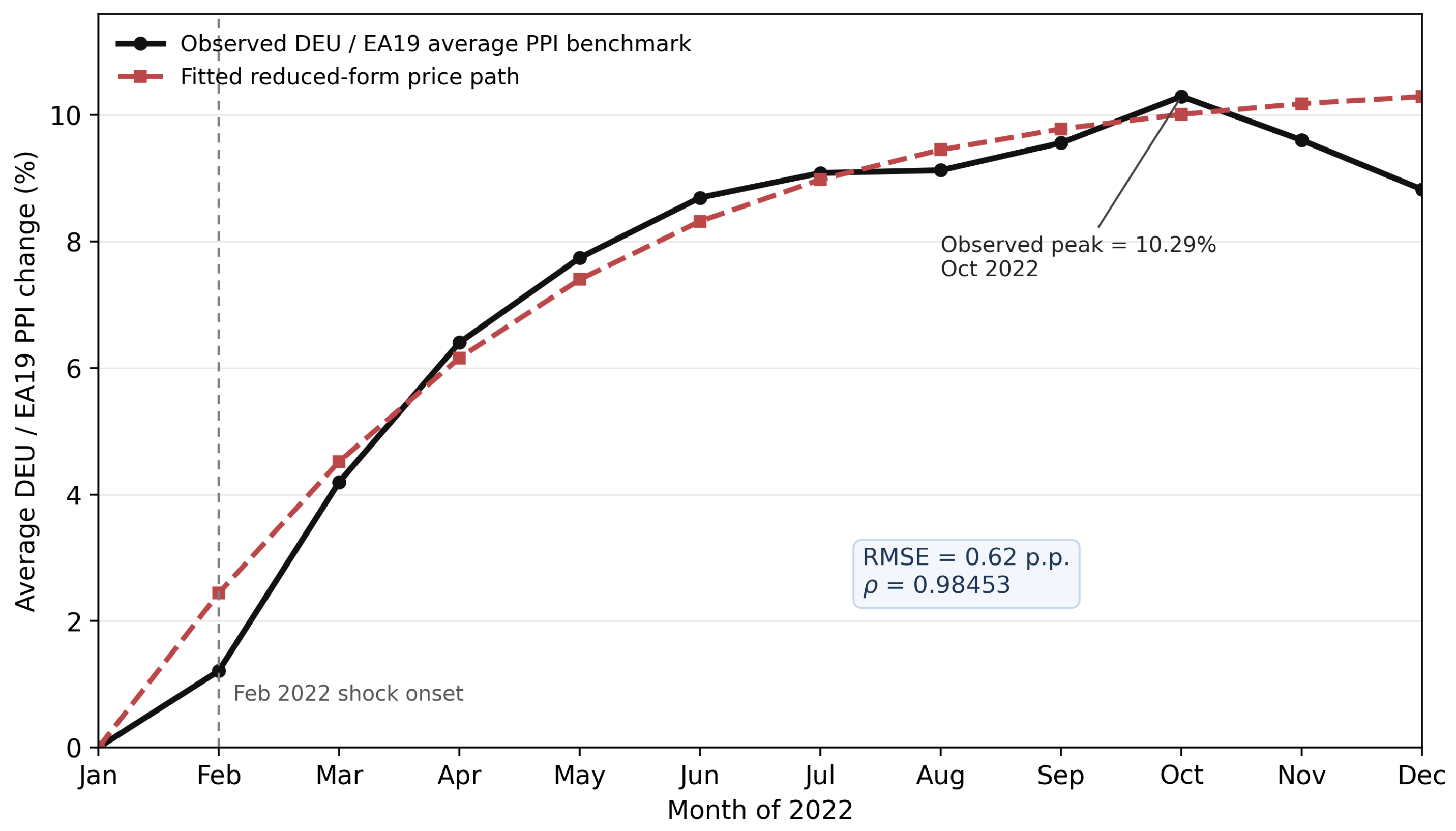
The separate price-validation layer is benchmarked against the 2022 Russia–Ukraine shock (Figure 1). Figure 1 plots a monthly OECD/FRED manufacturing PPI benchmark against the fitted reduced-form price path. The observed benchmark is constructed as the simple average of series PIEAMP01DEM661N for Germany and PIEAMP01EZM661N for EA19, normalized to January 2022, so the observed path peaks at 10.29% in October 2022. On the model side, the fitted reduced-form price path tracks that monthly benchmark with $RMSE=0.00623$ and $\rho =0.98453$. A simple holdout check based on fitting January–June 2022 and evaluating July–December yields a holdout error of about 1.92 percentage points.

For the Hormuz application itself, the event scale is bounded directly with first-quarter 2026 data [60,61]. Under that severe scenario, the model matches the quarter-end scale of the Brent price surge by month 2, though it front-loads the first-month pass-through to about 31.1%. The observed 2026 disruption lies above both the baseline and intervention thresholds reported below, which is why the policy comparison is framed as a resilience margin rather than as a claim that the event stayed inside the safe region.

3. Results

Unless otherwise stated, this section reports quantity-side output loss. Price pass-through is discussed separately. The results move from model comparison to the Hormuz stress test itself, then to the spatial and sectoral settlement of losses, the gas contrast case, the threshold geometry under alternative inventories, and the policy experiments.

3.1. Comparison with Reduced Baselines

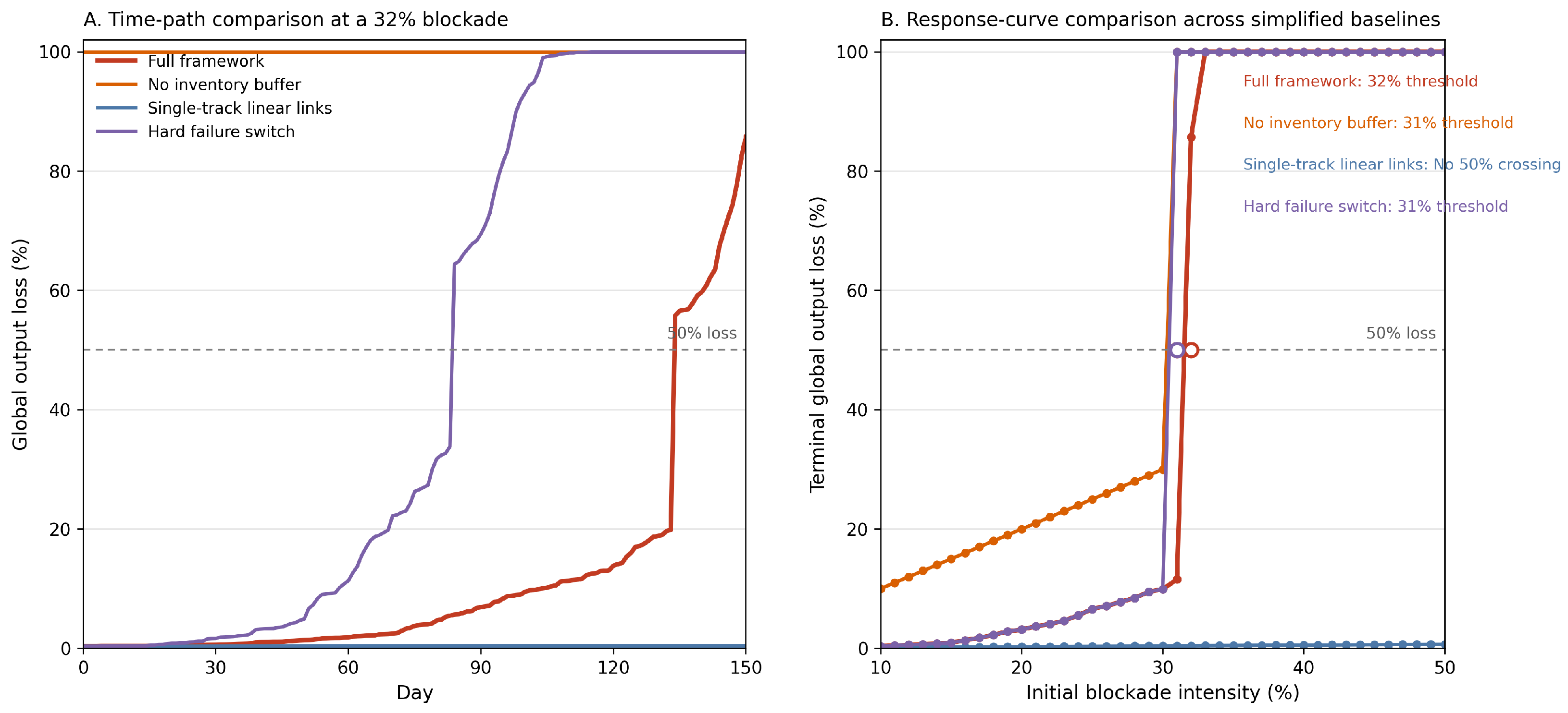
The role of each module becomes clear in a reduced-baseline comparison across the full specification and three reduced baselines, as shown in Figure 2: one without Edge-Level Inventories, one that collapses Dual-Track Dependence Topology into a single linear layer, and one that replaces Smooth Operability Bands with a hard-failure switch. The separate price-validation layer is kept outside this comparison because the object here is quantity-side cascade dynamics.

At a common 32% blockade, the full framework still exhibits a long accumulation window, as shown in Panel A of Figure 2. It does not cross 10% global output loss until day 104 and does not cross 50% until day 134. Removing edge-level inventories eliminates that window altogether. The no-inventory variant reaches both levels immediately because the targeted shortfall is transmitted without any stock buffer. Replacing smooth operability bands with a hard switch preserves some delay but sharpens the transition excessively, reaching 10% loss on day 58 and 50% on day 84. Collapsing the dual-track dependence topology into a single linear layer fails in a distinct way: the same 32% blockade produces only 0.43% terminal loss and never becomes a systemwide cascade inside the 150-day window.

The response-curve comparison leads to the same conclusion, as shown in Panel B of Figure 2. The full framework reaches the 50% terminal-loss threshold at 32% on the scan used here. The no-inventory and hard-failure baselines cross earlier, at 31%, but for different reasons: the former removes buffering, whereas the latter compresses the stress band into an on/off transition. The single-track linear variant never reaches 50% loss anywhere in the 10–50% blockade scan. The simplified models therefore fail in different ways. Only the full framework combines delayed transmission with a finite failure threshold that can be used for short-run resilience diagnosis.

3.2. Threshold Dynamics Under the Hormuz Stress Test

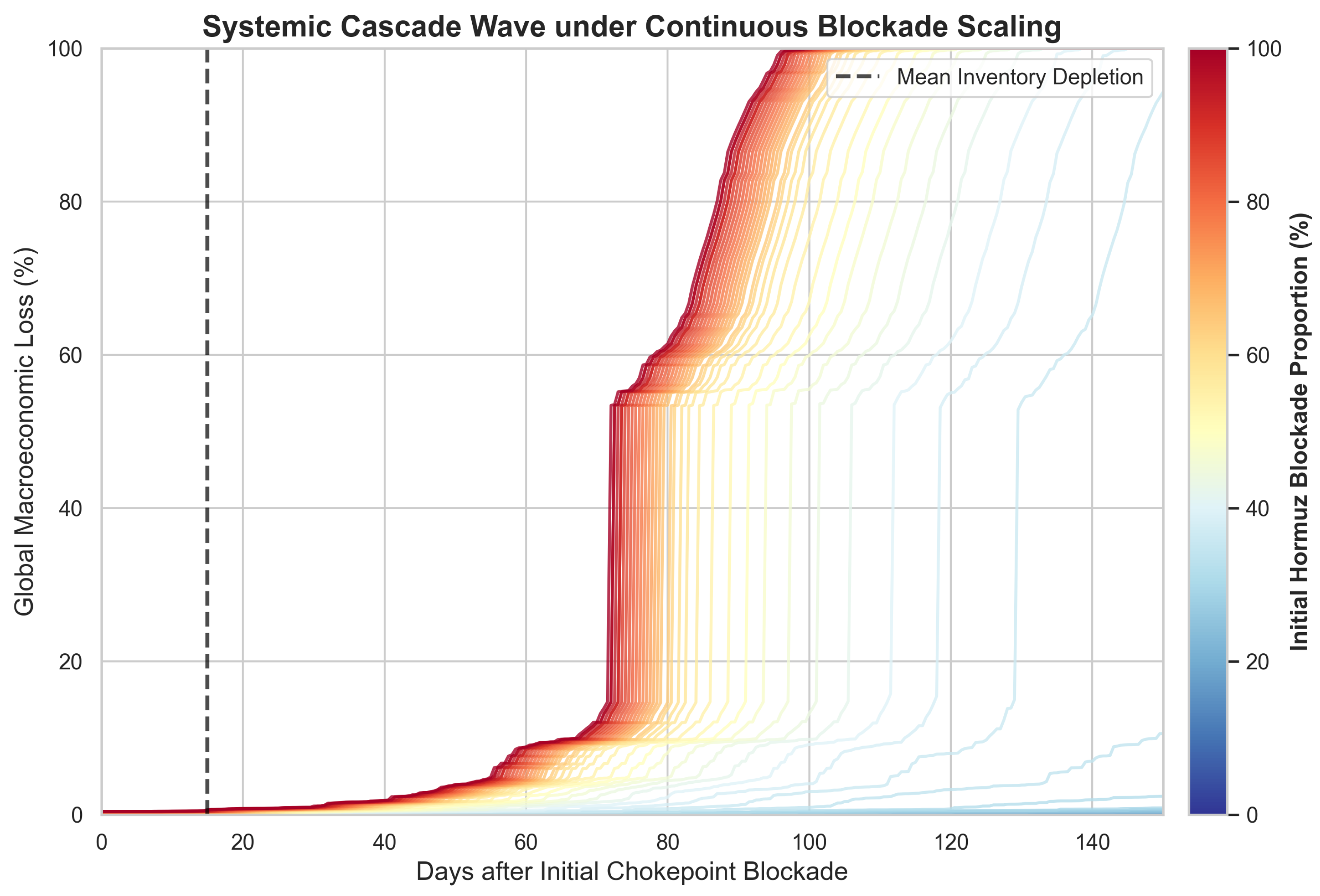
Under the Hormuz stress scenario, the system response takes the form of a long period of strain followed by a relatively narrow transition into collapse, as shown in Figure 3. A 20% blockade never reaches even 1% global output loss over the 150-day window and peaks at only 0.22%. The 32% case, which sits at the baseline threshold used later in the policy scan, still ends at only 2.39% by day 150. The 34% case remains in a stressed but not yet collapsed regime for most of the window and ends at 10.57%. At 40%, the trajectory changes qualitatively, and the system reaches 50% loss by day 112.

What matters here is not simply that larger shocks lead to larger losses. The response curve changes shape. At low intensities, the system stays in a low-loss regime for most of the horizon. Just beyond the transition, inventories across connected hubs are depleted in close succession, and local scarcity turns into faster cascade growth. The temporal evidence therefore matches the reduced-model comparison above: The system exhibits a delayed but finite transition band rather than a smooth proportional worsening.

The implication for interpretation is direct. Early stability is real, but it reflects temporary shielding rather than durable resilience. The system appears manageable until the same inventories that absorb the first wave are depleted. Once that happens, the accumulated stress is transmitted quickly through the rest of the network.

3.3. Cross-Economy and Cross-Sector Loss Concentration

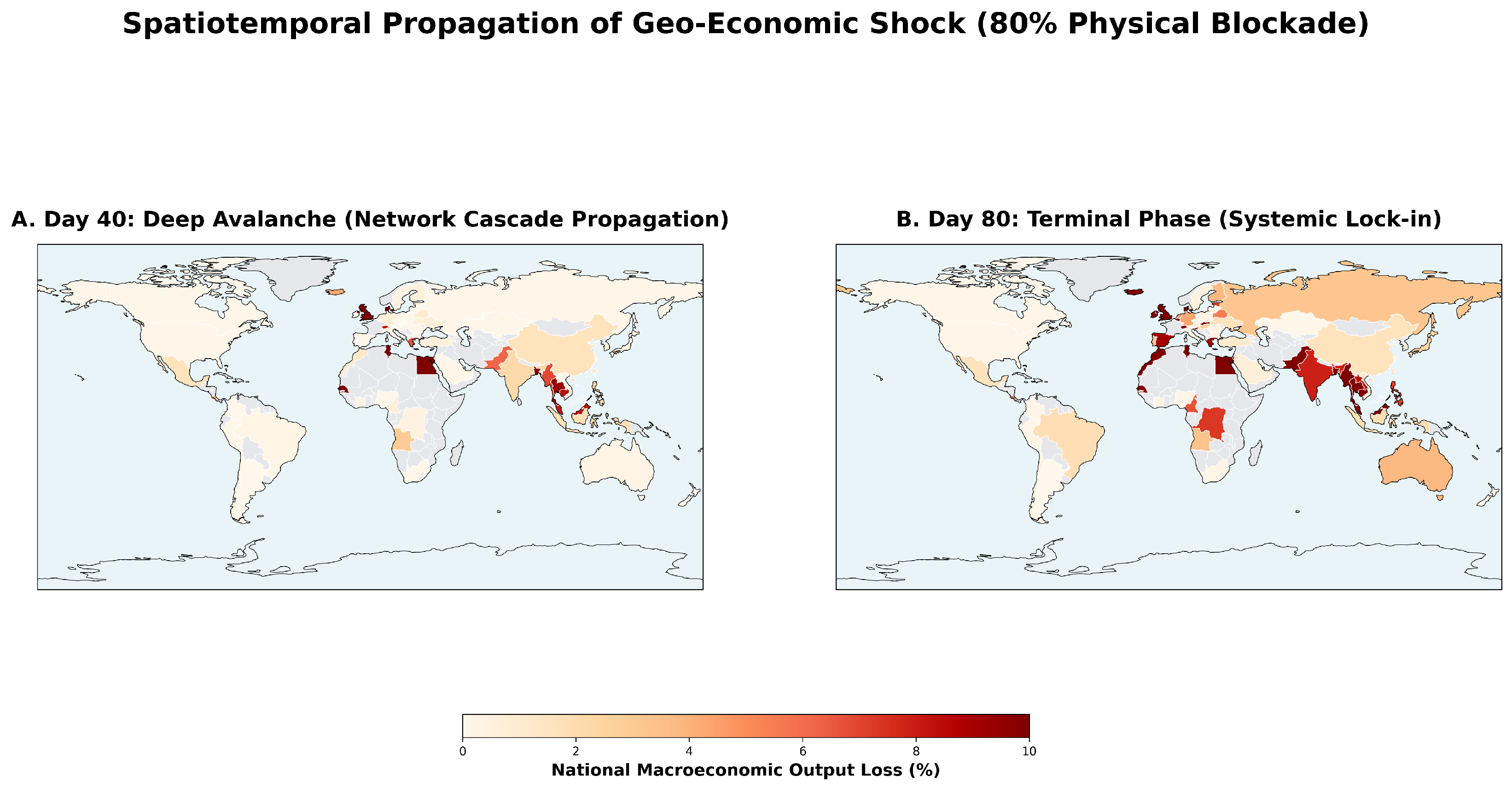
With the time structure identified, attention turns to where losses are concentrated. Which economies absorb the burden, and through which sectors is it transmitted? Figure 4 and Figure 5 jointly address these questions. The first operates at the geographic level. The second traces the sectoral transmission channels.

The key spatial pattern is a separation between origin and settlement. The disruption begins in Gulf energy and maritime nodes, yet the largest output losses do not remain there. They propagate into East and Southeast Asian manufacturing supply chains and, at the terminal stage, are absorbed disproportionately by major downstream consumer markets. Economies such as China, Vietnam, and South Korea sit inside dense manufacturing chains that require repeated border crossings of intermediates before final assembly, so stress arrives from several upstream directions at once. Large final-demand markets, especially China and the United States, then absorb a substantial share of the output loss because they lie below the most stressed midstream sectors in the final-demand matrix.

The map is therefore not a simple picture of direct import dependence. It is a map of network settlement. Countries that appear distant from the chokepoint can still bear substantial losses if they lie below overloaded industrial relays. Direct exposure alone does not account for the final burden pattern reported here.

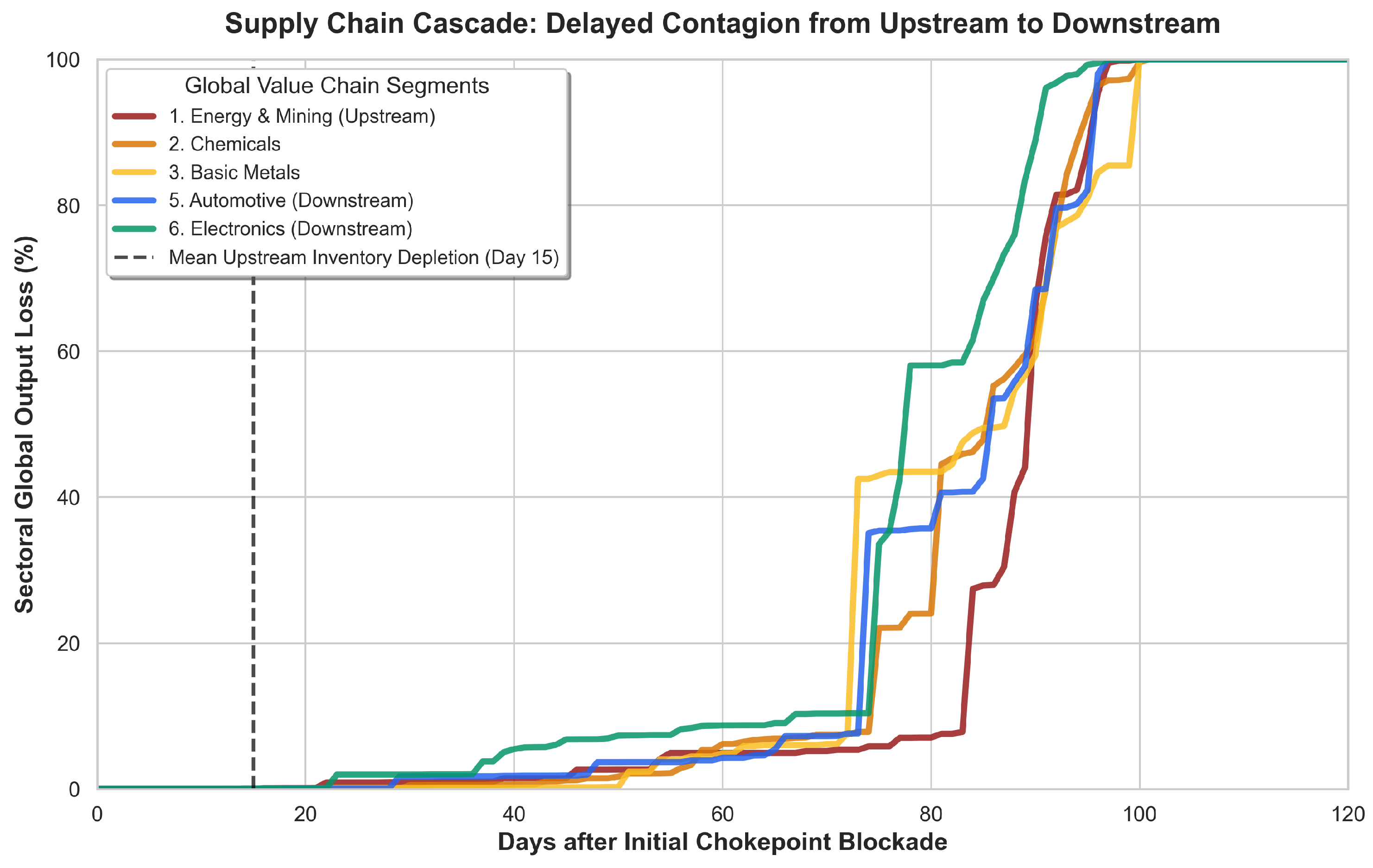
The sectoral view points to a concentrated set of relay sectors, as shown in Figure 5. The cascade does not move evenly across industries. Utilities, petrochemicals, basic metals, and air transport emerge as the dominant relay sectors. That ranking follows directly from the structure of the shock. These sectors depend heavily on energy-intensive or logistics-sensitive inputs, are difficult to substitute in the short run, and connect upstream scarcity to broad downstream production loss.

Utilities are central because fuel stress there becomes an economy-wide operating constraint. Petrochemicals sit close to Gulf feedstocks and also feed a wide range of manufacturing supply chains. Basic metals translate energy and shipping stress into material bottlenecks for construction, machinery, and fabricated manufactures. Air transport matters for a different reason: once maritime routes are impaired, part of the high-value flow is diverted into air freight just as jet fuel and rerouting costs rise. A channel that initially serves as a substitution soon becomes another bottleneck.

The geographic and sectoral results describe the same mechanism at two resolutions. The map identifies where losses are concentrated, and the sector figure identifies the sectors through which they are transmitted. Nearby-parameter checks indicate that the top relay group is stable for utilities and petrochemicals, while some lower-order relay positions are more sensitive to buffering and bottleneck classification.

3.4. Gas Comparison

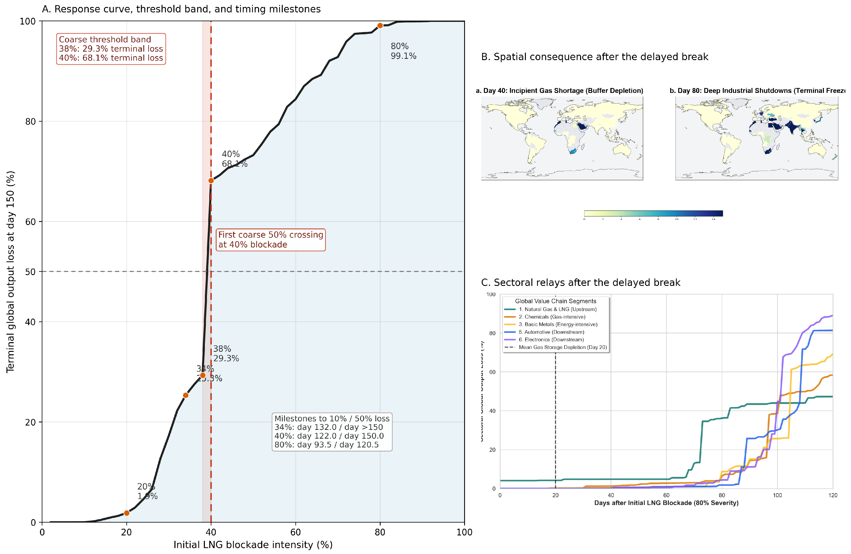
The gas case keeps the threshold-cascade logic fixed while changing three ingredients at once: the shock bundle is narrower, storage is deeper, and the operability bands are tighter for gas-sensitive sectors. Figure 6 compares the threshold curve in Panel A with the downstream consequences in Panels B and C. Under this gas configuration, the 50% terminal-loss crossing does not appear at 38% blockade, where terminal loss is 29.33%, and first appears at 40%, where terminal loss reaches 68.14% by day 150. The gas threshold therefore lies between 38% and 40% on the coarse scan used here. Below that interval, losses are materially lower than in the combined oil-shipping case: a 20% LNG blockade ends at 1.85% global output loss, and a 34% blockade ends at 25.33%. Above it, the post-threshold rise is still steep: terminal loss reaches 73.21% at 50% blockade and 99.07% at 80%.

The time paths reinforce that comparison. Under a 34% LNG blockade, the gas-only case reaches 1%, 5%, and 10% loss only on days 87.5, 122.5, and 132.0, and it never reaches 50% within the simulated horizon. At 40%, those milestones arrive earlier, on days 79.0, 113.0, and 122.0, and the 50% mark appears only at day 150. At 80%, the 50% mark appears on day 120.5. The gas case, therefore, provides more warning time than the combined oil-shipping scenario, but once storage buffers are exhausted, the late-stage deterioration is still abrupt.

After the threshold is crossed, losses concentrate in economies tied to gas-sensitive utilities and industrial relays. At 80% blockade, the spatial burden extends well beyond the immediate origin of the supply disruption. The sectoral panel shows a similar concentration along transmission channels: upstream gas and LNG, gas-intensive chemicals, basic metals, and downstream manufacturing relays absorb disproportionate losses once storage is exhausted. This comparison does not claim to be a full oil–gas system. It isolates the timing and consequence structure of a storage-sensitive gas shock under the same cascade logic.

3.5. Inventory, Calibration, and Threshold Placement

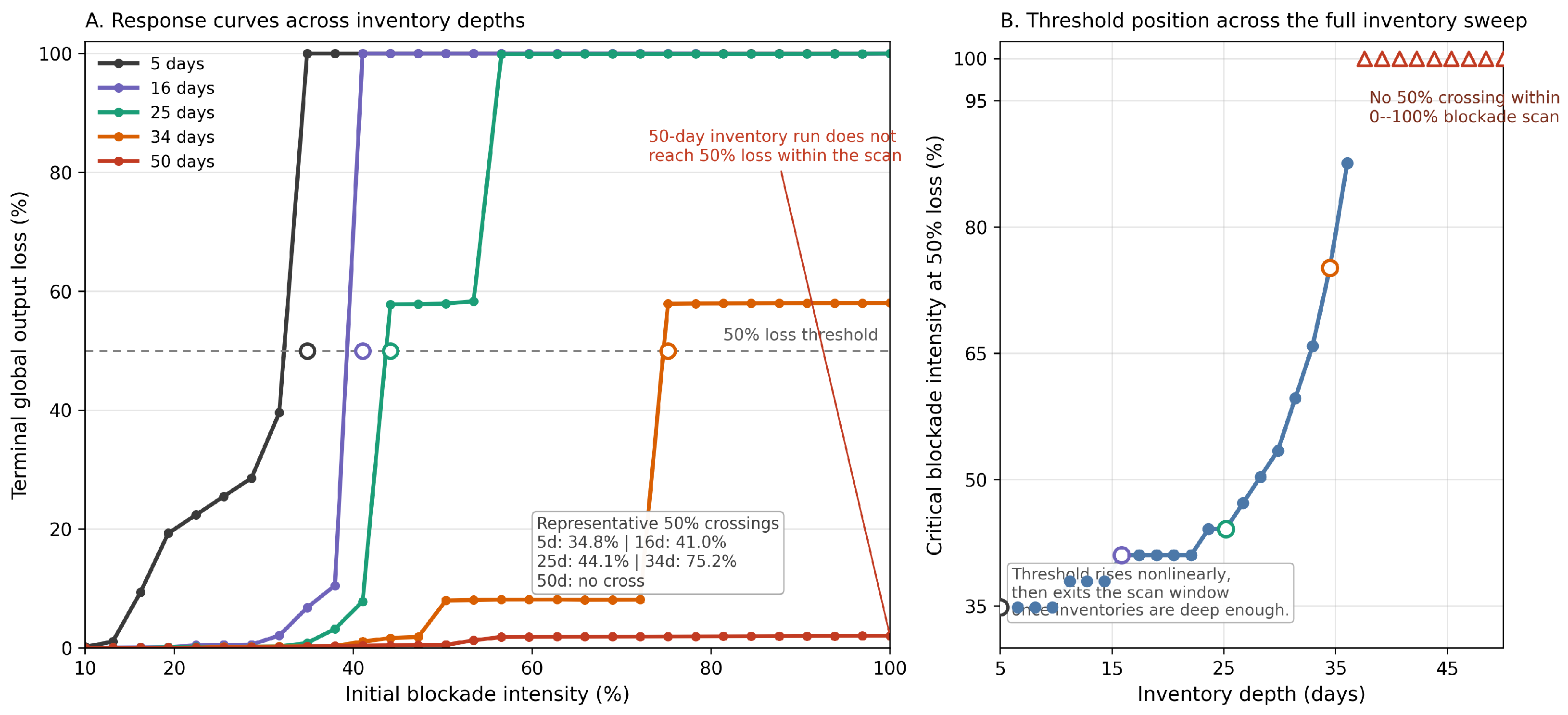
Having located the break and tracked its consequences, the next step is to ask what determines the threshold. Inventory depth changes where collapse begins, not how steeply losses rise once the system is already beyond the bend, as shown in Figure 7. In the response curves of Panel A, the five-day run crosses the 50% loss line at about 34.8% blockade intensity. At roughly 16 days, the crossing shifts to about 41.0%. At roughly 25 days, it shifts to about 44.1%. At roughly 34 days, it shifts much further, to about 75.2%. In the 50-day run, the curve never reaches the 50% line anywhere within the 0–100% blockade sweep.

The relation between inventory depth and threshold position is monotonic but distinctly nonlinear, as shown in Panel B of Figure 7. Over low and moderate inventory depths, the threshold rises in steps from roughly 34.8% to 53.4%. Once inventories move above about 30 days, the curve steepens sharply: the threshold rises to about 59.7%, then 65.9%, then 75.2%, and reaches about 87.6% by roughly 36 days. Beyond about 37.6 days, no 50% crossing appears within the diagnostic scan. These values are comparative threshold positions across inventory settings. They are not a replacement for the baseline Hormuz threshold reported below.

The connection to the earlier figures is direct. The temporal curves showed that the system can remain quiet for a long interval before collapsing. The inventory sweep shows why. Deeper inventories widen the buffered region and push the crossing point rightward, but the transition is still abrupt once the relevant stocks are exhausted. Inventory therefore changes how much shock the system can absorb before failure. It does not make the failure regime linear.

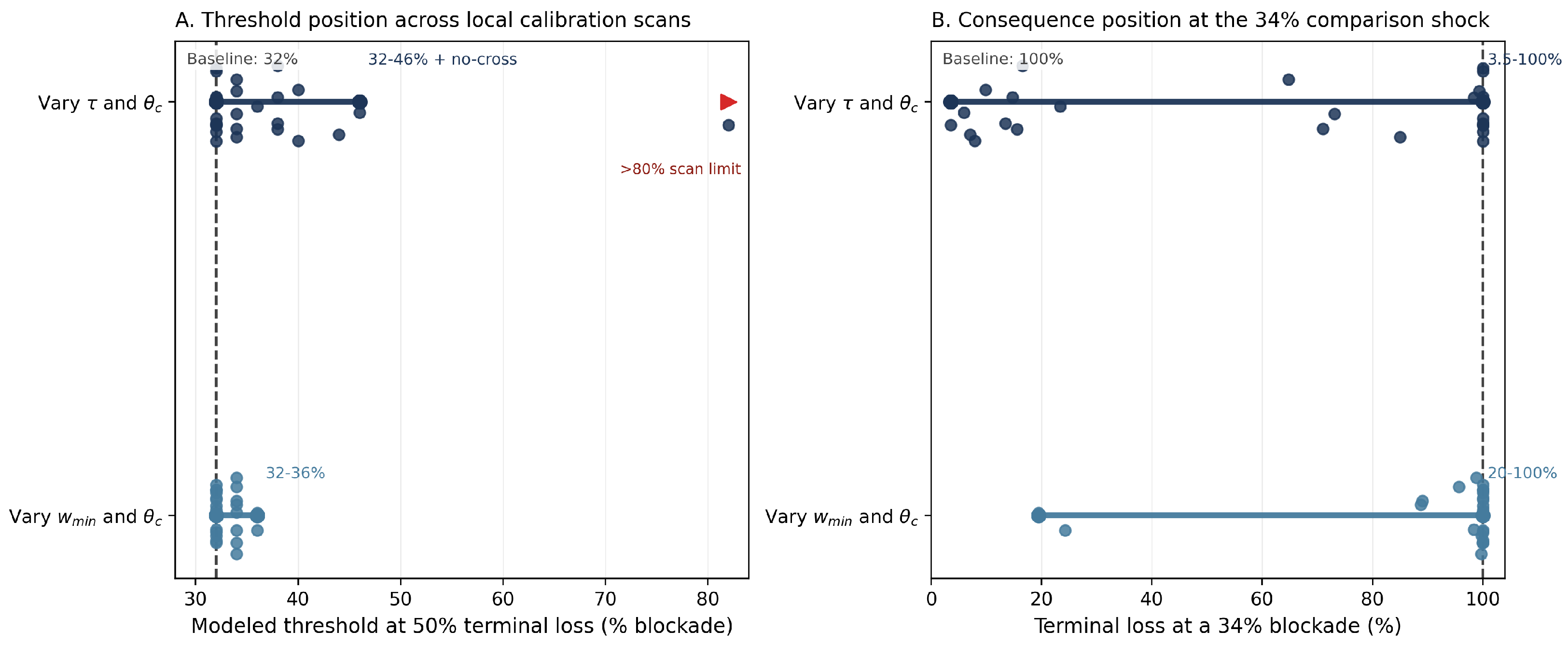
Figure 8 compresses the main local calibration evidence into two scan families. When $\tau$ and ${\theta }_c$ vary together, the threshold spans 32–46%, and one upper-corner specification does not cross 50% loss anywhere within the scanned blockade range. When $w_{min}$ and ${\theta }_c$ vary together, the threshold stays clustered at 32–36%. At a common 34% blockade, terminal loss spans 3.5–100% across the $\tau \times {\theta }_c$ family but 20–100% across the $w_{min}\times {\theta }_c$ family. The dominant sensitivity therefore comes from assumptions that govern buffer exhaustion and hard-bottleneck classification rather than from moderate changes in network sparsification.

The modeled threshold also depends on the horizon over the 90–210 day window. Shortening the simulation horizon from 150 to 90 days shifts the 50% threshold from 32% to 38%, and terminal loss at a common 34% blockade falls from 100% to 16.3%. At 120 days, the threshold is 34%. Once the horizon reaches 150 days, the threshold stays at 32% throughout the 150–210-day scan. The main-text calibration picture is therefore stable in ordering even though the exact threshold value depends on horizon and buffering assumptions.

3.6. Which Interventions Shift the Failure Threshold

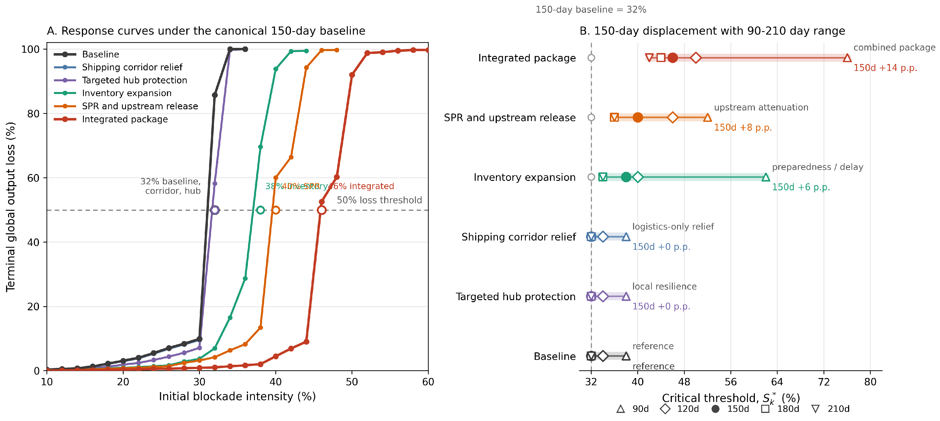
The last question in the Section 3 is policy-relevant: Which interventions materially delay systemic failure, and by how much? Figure 9 compares interventions by how far they shift the blockade intensity required to produce 50% terminal global output loss. Inventory expansion deepens buffers. Strategic Petroleum Reserve (SPR) plus upstream release attenuates upstream scarcity once the event is under way. Shipping-corridor relief acts only on transport friction, and targeted hub protection acts only on local resilience at selected nodes. The integrated package combines all four channels.

The intervention effect is mainly horizontal: the transition moves to the right more than the post-threshold rise is flattened, as shown in Panel A of Figure 9. Under the baseline calibration, the system crosses the 50% line at 32% blockade intensity. Shipping-corridor relief and targeted hub protection also cross at 32% on this scan. Inventory expansion delays the crossing to 38%, and Strategic Petroleum Reserve (SPR) plus upstream release delays it to 40%. The integrated package keeps losses low through a substantially wider shock range and does not cross the 50% line until 46%.

The gain appears earlier, in how much blockade intensity the system can absorb before it tips into systemic failure. That threshold comparison is summarized in Panel B of Figure 9: the filled marker denotes the baseline 150-day threshold, the open markers show each policy under alternative 90–210 day horizons, and the horizontal span shows the full short-run range. On the 150-day baseline, the integrated package yields the largest rightward shift, at +14 percentage points. Strategic Petroleum Reserve (SPR) plus upstream release yields +8 points, and inventory expansion yields +6. Shipping relief alone and targeted hub protection alone do not move the critical threshold on this calibration.

The horizon markers also show which parts of the ranking are stable. The strongest and weakest policies are stable across the 90–210 day window: the integrated package is always furthest to the right, and shipping-corridor-only and targeted-hub-only interventions stay close to the baseline. The middle pair is horizon-dependent. At 90 days, inventory expansion pushes the threshold to 62%, compared with 52% under SPR plus upstream release, because the shorter window rewards delay more strongly than attenuation. Once the horizon reaches 120 days, that ordering reverses. SPR plus upstream release moves the threshold further right than inventory expansion at 120 days (46% versus 40%), 150 days (40% versus 38%), and 180–210 days (36% versus 34%). The central policy ordering is, therefore, already visible in the main-text horizon scan.

4. Discussion

This study develops a threshold-cascade model for near-term production failure under maritime-energy disruption. The central result is a delayed but finite transition: inventories absorb the early shock, but once bottlenecks align, losses rise rapidly across the production network. The reduced-model comparison shows why the four-component structure matters. Removing edge-level inventories eliminates the buffered interval. Compressing dual-track dependence topology into a single linear layer largely removes the systemic threshold. Replacing smooth operability bands with a hard switch preserves delay but pushes the break earlier and makes it too abrupt [12,18,22,29,30,46]. These comparisons identify a model object with a clear interpretation: the blockade intensity at which the short-run quantity system crosses a stated loss convention under explicit buffering and bottleneck assumptions.

The mathematical contribution lies in a defined recursive state system and in the threshold functionals read from it. Section 2 specifies the one-step map ${\mathsf{\Phi }}_{k,\mathsf{\Theta },S_0}$ on the state vector ${\mathbf{z}}^{\left(t\right)}$. Section 3 reports observables derived from that same trajectory. The temporal curves come from the path $L_{out}^{\left(k\right)}(t;S_0,\mathsf{\Theta })$. The response-curve and policy panels come from the sampled terminal map $S_0\mapsto R_k(S_0;\mathsf{\Theta },T)$. The threshold markers are the induced crossing statistic $S_k^{*}(0.5;\mathsf{\Theta },T)$. The country map and sector figure are terminal aggregations of the same simulated node-level losses. This is why the figures are directly tied to the equations rather than being generated by a separate empirical procedure.

The baseline threshold should nevertheless be read as a bounded estimate, not as a structural constant. Under the baseline 150-day setup, the coarse scan places the first 50% crossing at 32%, and the local calibration scans place the broader range at 32–46% once buffer depth and hard-bottleneck classification are varied. Horizon changes move the threshold to 34% at 120 days and to 38% at 90 days. Additional seed and network-vintage checks widen the range further, although they do not overturn the qualitative ordering. The reported threshold is therefore a short-run diagnostic under a stated setup, not a horizon-free property of the world economy.

Two limitations deserve explicit emphasis. The first is the one-way price layer. The reduced-form price block is used only to benchmark the size and timing of the price pulse against observed producer-price data. It does not feed back into quantity decisions. As a result, the model does not capture the possibility that very high prices induce demand destruction, substitution, or deliberate production cuts that partly slow the cascade. In severe price states, the present setup can, therefore, overstate physical production failure relative to a fully coupled price-quantity system.

The second limitation is the network latency. The production network is built on the 2022 benchmark year extracted from the 2025 edition of OECD ICIO. That is the latest harmonized cross-country benchmark available in this framework, but it is still a dated representation of global production structure. If near-shoring, trade diversion, or geopolitical realignment materially rewired supplier dependence after 2022, some bottlenecks and relay positions could shift by 2026. Simple network-vintage perturbations are useful as stress tests, but they are not a substitute for re-estimating the model on a newer benchmark table once one becomes available.

Within those limits, the policy result is still informative. Inventory support and partial upstream release help, but they do not move the threshold as far as an integrated package that acts on multiple constraints at once. Measures aimed at a single local friction stay weak when the transition is jointly governed by upstream scarcity, finite inventories, and midstream overload. The strongest and weakest interventions are stable across the 90–210 day window, although the ordering between inventory expansion and SPR plus upstream release depends on disruption duration.

Future work should proceed in three directions. First, the one-way price-validation layer should be extended to a controlled two-way price-quantity feedback system so that demand destruction and substitution can alter the propagation path. Second, the route-level shipping representation should be made more explicit, rather than being proxied through throughput and delay penalties alone. Third, the same framework should be updated with newer cross-country input-output benchmarks and applied to additional chokepoints so that the extent of setting-specific versus portable threshold logic can be assessed more directly.

5. Conclusions

Abrupt maritime-energy disruption can generate near-term production failure before substitution or contract adjustment dominates. This study develops a threshold-cascade framework that combines dual-track dependence topology, edge-level inventories, and smooth operability bands, while keeping price validation separate from quantity loss.

In the Strait of Hormuz stress test, three findings stand out. The first is temporal: inventories delay failure, but once blockade intensity moves past roughly 32% under the baseline 150-day horizon, losses rise quickly. The second is spatial and sectoral: the burden does not stay at the point of origin. It is amplified through East and Southeast Asian manufacturing supply chains and relayed through utilities, petrochemicals, basic metals, and air transport. The third is policy-related: single-channel measures shift the threshold only modestly, whereas the integrated package moves it from 32% to about 46% in this calibration.

The contribution is therefore specific. It is not a long-run equilibrium model, and it is not a complete oil-price model. It is a short-run diagnostic for identifying when buffers fail, where losses settle, and which intervention packages delay systemic disruption under explicit physical constraints. The current estimates depend on the 2022 benchmark network, the one-way price treatment, the simulation horizon, and the terminal-loss convention. Those limitations matter. Even so, the framework provides a tractable basis for comparing near-term resilience under abrupt maritime-energy disruption, and it gives a clear agenda for extending the model in the next round.