On the Diminished Sombor Index of Bipartite Graphs of Fixed Diameter

Abstract

The diminished Sombor index is a degree-based topological index that normalizes the Sombor contribution of each edge (defined as the Euclidean norm of the endpoint degrees) by the sum of those degrees, thereby making the index independent of graph size and ensuring a more balanced reflection of the relative degree contributions of adjacent vertices. In this paper, we investigate the extremal behavior of the diminished Sombor index over the class of connected bipartite graphs with fixed order and diameter. We establish a sharp upper bound for this index within the family of all bipartite graphs on a given number of vertices and with a prescribed diameter, and we completely characterize the extremal graphs attaining this bound. Furthermore, we prove that the maximum diminished Sombor index strictly decreases as the diameter increases. As a consequence, we determine the connected bipartite graphs of fixed order that achieve the three largest values of the diminished Sombor index.

1. Introduction

Let $G=\left(V\right(G),E(G\left)\right)$ be a simple connected graph. For a vertex $u\in V\left(G\right)$, its neighborhood is defined by $N_G\left(u\right)=\{v\in V\left(G\right):uv\in E\left(G\right)\}$, and the degree of u is $d_G\left(u\right)=\left|N_G\left(u\right)\right|$. The distance between two vertices u and v is denoted by $d(u,v)$, and the diameter of G is defined as $d=max\left\{d\right(u,v):u,v\in V(G\left)\right\}.$ The path on n vertices and the complete bipartite graph are denoted by $P_n$ and $K_{a,n-a}$, respectively. All notations and terminology used in this paper follow the conventions in [1].

Topological indices are numerical descriptors of graphs and are frequently used to model molecular properties in chemical structures. These indices play a significant role in determining structure–property and structure–activity relationships. Recently, new approaches that aim to limit the influence of high-degree vertices and provide more results have attracted considerable attention [2]. The Sombor index, a prominent topological index in graph theory, was introduced in [3] and is defined as

$$SO\left(G\right)=\sum _{uv\in E\left(G\right)}\sqrt{d_u^2+d_v^2}.$$

It has attracted considerable attention for its applications in quantitative structure–property and structure–activity relationship (QSPR/QSAR) studies. Liu et al. [4] reviewed existing bounds and extremal results for the Sombor index and its variants. Movahedi and Akhbari [5] computed exact formulas for several Sombor-type topological indices of hyaluronic acid–methotrexate conjugates used in cancer treatment. Zhou et al. [6] characterized trees and unicyclic graphs with minimum Sombor index among graphs with given maximum degree. Movahedi and Akhbari [7] introduced the entire Sombor index and established various bounds for it. Liu et al. [8] determined extremal (reduced) Sombor index values for chemical trees and showed that boiling points of benzenoid hydrocarbons are highly correlated with these indices. Movahedi et al. [9] applied topological indices and data analysis techniques to model physicochemical properties of tetracycline antibiotics. Samiei and Movahedi [10] investigated graph invariants for predicting properties of chemical structures of antiviral drugs. More recently, a variant known as the diminished Sombor index was first proposed in [11] and referred to by this name in [12]. This index is defined as follows

$$DSO\left(G\right)=\sum _{uv\in E\left(G\right)}{\displaystyle \frac{\sqrt{d_u^2+d_v^2}}{d_u+d_v}}.$$

In their study, Movahedi et al. [12] established various bounds for the diminished Sombor (DSO) index, characterized extremal graphs, and formulated inequalities analogous to those of the Nordhaus–Gaddum type. They also conducted numerical investigations to explore how the DSO index varies with structural features, highlighting its possible applications in chemistry. Furthermore, in [13], the tricyclic graph of a given order that achieves the maximum DSO value was identified, along with an analysis of its unique structural properties. Subsequently, the conjecture concerning tricyclic graphs minimizing the DSO index was resolved in [14], where the extremal structures attaining the minimum value were completely characterized. In addition, the work presented in [15] investigated the relationship between the DSO index and several classical degree-based topological indices, establishing sharp bounds including $DSO\left(G\right)\le {\displaystyle \frac{\sqrt{2}}{2}}(Alb\left(G\right)+m)$, where $Alb\left(G\right)={\sum }_{uv\in E}|d_u-d_v|$ is the Albertson index and $m=\left|E\right(G\left)\right|$, as well as bounds in terms of the maximum degree $\Delta$, minimum degree $\delta$, and the size m of the graph.

In recent years, significant progress has been made in the study of Sombor-type indices, particularly in determining extremal values for various graph classes. Cruz and Rada [16] determined extremal values of the Sombor index in unicyclic and bicyclic graphs. Cruz, Gutman and Rada [17] characterized the extremal graphs with respect to the Sombor index over chemical graphs, chemical trees, and hexagonal systems. Das and Gutman [18] investigated the Sombor index of trees. Liu [19] determined extremal values of the Sombor index for unicyclic graphs with a given diameter. Sun and Du [20] determined the Sombor index of trees with fixed domination number. For trees, extremal results have been extensively developed under structural constraints such as fixed order, diameter, and matching number. In the case of unicyclic and bicyclic graphs, the presence of cycles introduces additional structural complexity, and extremal configurations are typically obtained through degree-based transformations and edge-redistribution techniques. Khanra and Das [21] determined extremal values of the Euler Sombor index for trees and unicyclic and chemical graphs, and proposed several open problems. Kizilirmak [22] derived the minimum Euler Sombor index for unicyclic graphs with fixed diameter. Ali et al. [23] established the best possible bounds for graphical edge-weight-function indices of trees under constraints on matching number, number of pendent vertices and maximum degree, with applications to the Euler Sombor index. Tache et al. [24] determined extremal unicyclic graphs for the Euler Sombor index.

These approaches have been further extended to more complex graph families. Hu et al. [25] obtained bounds on the Euler Sombor index of maximal outerplanar graphs. Kizilirmak [26] determined the extremal values of the Euler Sombor index of tricyclic graphs. Ren et al. [27] investigated the Euler Sombor index of trees. In addition to the classical Sombor index, several variants have been investigated. Zhang et al. [28] obtained bounds for the Euler Sombor index of molecular trees and its applications. Albalahi et al. [29] characterized graphs attaining optimal values of the Euler Sombor index among all molecular tricyclic graphs. Su and Tang [30] determined maximal and minimal values of the Euler Sombor index for unicyclic and bicyclic graphs. Das and Bera [31] resolved two open problems on the Euler Sombor index concerning extremal graphs with fixed girth and given number of pendant vertices. Das, Mondal and Pal [32] determined extremal trees for the Euler Sombor index with given parameters.

Motivated by the growing body of work on extremal Sombor-type indices under structural constraints, it is natural to investigate how global metric parameters, such as the diameter, influence the behavior of these indices. While many existing studies focus on local properties, including degree sequences, matching number, and connectivity, comparatively less attention has been given to the role of distance-based parameters in shaping extremal configurations. Since the diameter imposes a layered structure on the graph and significantly affects vertex interactions, it provides a meaningful framework for analyzing the diminished Sombor index from a different perspective.

Recently, the two-scale fractal dimension has emerged as a powerful tool for characterizing the spatial geometric complexity of molecular and network structures. Unlike classical fractal dimensions, it effectively captures both self-similar and non-self-similar structures, making it widely applicable in structural description [33,34].

In chemical applications, the two-scale fractal dimension mainly captures the spatial geometric complexity of molecules. The key difference between the two-scale fractal dimension and the degree-based DSO index is that the former focuses on spatial geometry, while the latter emphasizes vertex degree distribution and local edge contributions. Thus, they are complementary rather than substitutable. To illustrate this distinction, consider the path graph $P_4$ on four vertices $v_1,v_2,v_3,v_4$ with edges $v_1{v}_2,v_2{v}_3,v_3{v}_4$. The degrees are $d_{v_1}=d_{v_4}=1$ and $d_{v_2}=d_{v_3}=2$, and the DSO index is computed edge by edge as follows:

$$DSO\left(P_4\right)=2{\displaystyle \frac{\sqrt{1^2+2^2}}{1+2}}+{\displaystyle \frac{\sqrt{2^2+2^2}}{2+2}}={\displaystyle \frac{2\sqrt{5}}{3}}+{\displaystyle \frac{\sqrt{2}}{2}}\approx 2.199.$$

This value reflects the degree imbalance at terminal versus internal vertices. In contrast, the two-scale fractal dimension of the same linear chain characterizes its self-similar spatial extension along one dimension. Changing the chain length affects the fractal dimension continuously, while the DSO index changes discretely as new edges and degrees are introduced. The two descriptors thus provide complementary structural information, and neither can substitute for the other. The main contributions of this paper are as follows. First, we establish a sharp upper bound for the DSO index over the class ${\mathcal{B}}_n^d$ of connected bipartite graphs with fixed order and diameter, and completely characterize all extremal graphs attaining this bound. Second, we prove that the maximum DSO index over ${\mathcal{B}}_n^d$ is strictly decreasing as the diameter increases. Third, as a consequence, we determine the connected bipartite graphs of fixed order achieving the three largest DSO values. While extremal problems for degree-based indices under degree-sequence constraints are well studied, the role of diameter as a structural parameter in shaping extremal configurations for normalized Sombor-type indices has not been previously investigated.

2. Characterization of Graphs with Maximal Diminished Sombor Index

For each $G\in {\mathcal{B}}_n^d$, there exists a partition of the vertex set $V\left(G\right)$ into subsets $T_0,T_1,\dots ,T_d$, where $T_0=\left\{v\right\}$ for some fixed vertex v, and for each $i=1,2,\dots ,d$, we define

$$T_i=\{w\in V\left(G\right):d(v,w)=i\}.$$

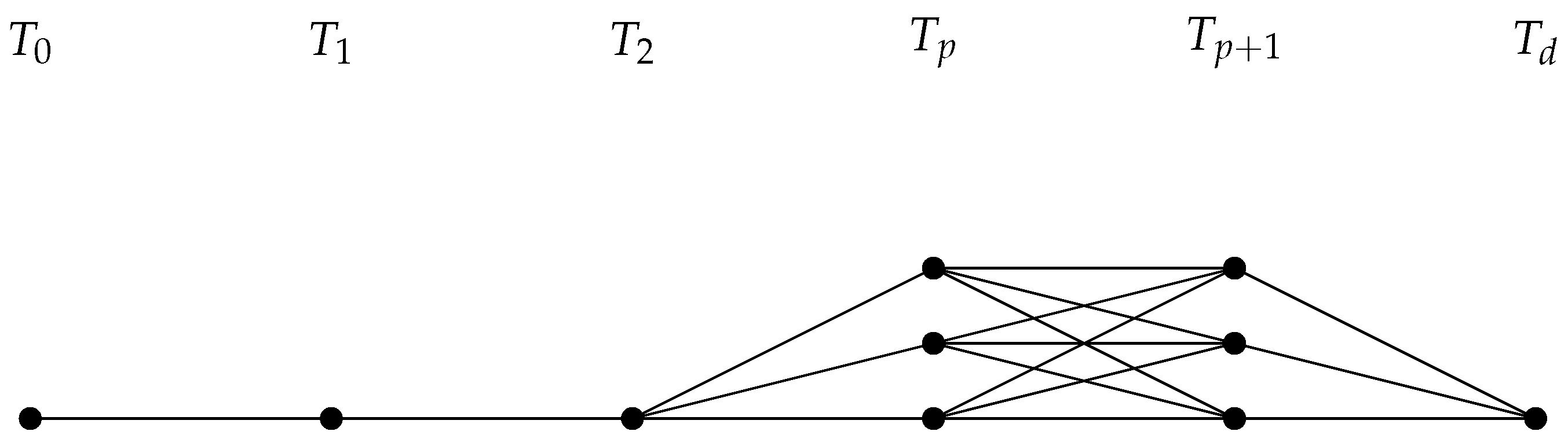
Each $T_i$ is called a partition set, and we denote $m_i=\left|T_i\right|$ for $i=1,2,\dots ,d$. The vertex partition $T_0,T_1,\dots ,T_d$ induces a layered structure on the graph, where each set $T_i$ consists of vertices at distance i from a fixed root vertex. By construction, no edges exist within the same layer, and edges may occur only between consecutive layers. In the extremal case, this structure becomes highly organized: most layers contain a single vertex, while at most two adjacent layers may contain multiple vertices, forming a complete bipartite subgraph. This layered configuration plays a central role in the analysis of the diminished Sombor index. This structure is illustrated in Figure 1.

Lemma 1

([12]). Let $\gamma (x,y)={\displaystyle \frac{\sqrt{x^2+y^2}}{x+y}},$ where $x,y>0$. Then for $x>y$, the function $\gamma (x,y)$ is strictly increasing with respect to x and strictly decreasing with respect to y. Moreover, for $x=y$ one has $\gamma (x,x)={\displaystyle \frac{1}{\sqrt{2}}}$.

Lemma 2.

Let $\eta (x,y)=\gamma (x,y)-\gamma (x-1,y)$, where $x\ge 2$, $y\ge 1$. Then $\eta (x,y)$ is strictly increasing with respect to x, and strictly decreasing with respect to y.

Proof. 

By definition, we have

$$\eta (x,y)=\gamma (x,y)-\gamma (x-1,y),$$

and from Lemma 1, it follows that $\gamma (x,y)>\gamma (x-1,y)$ for $x\ge 2$, $y\ge 1$. Hence, $\eta (x,y)>0$.

By direct calculation, one may obtain

$${\eta }_x(x,y)={\displaystyle \frac{\partial \gamma }{\partial x}}(x,y)-{\displaystyle \frac{\partial \gamma }{\partial x}}(x-1,y)={\displaystyle \frac{y(x-y)}{{(x+y)}^2\sqrt{x^2+y^2}}}-{\displaystyle \frac{y(x-1-y)}{{(x+y-1)}^2\sqrt{{(x-1)}^2+y^2}}}>0,$$

which shows that $\eta (x,y)$ is strictly increasing in x.

$${\eta }_y(x,y)={\displaystyle \frac{\partial \gamma }{\partial y}}(x,y)-{\displaystyle \frac{\partial \gamma }{\partial y}}(x-1,y)=-{\displaystyle \frac{x(x-y)}{{(x+y)}^2\sqrt{x^2+y^2}}}+{\displaystyle \frac{(x-1)(x-1-y)}{{(x+y-1)}^2\sqrt{{(x-1)}^2+y^2}}}<0,$$

so $\eta (x,y)$ is strictly decreasing in y.

This completes the proof. □

Lemma 3

([35]). For any graph $G\in {\mathcal{B}}_n^d$ with the above partition of $V\left(G\right)$, the induced subgraph $G\left[T_i\right]$ is an empty graph (i.e., contains no edge) for each $i\in \{0,1,\dots ,d\}$.

Lemma 4.

Let $G\in {\mathcal{B}}_n^d$ be a graph with the maximal $DSO$ value. Then $G[T_{i-1}\cup T_i]$ induces a complete bipartite subgraph for each $i\in \{1,2,\dots ,d\}$, and $|T_d|=1$ whenever $d\ge 3$.

Proof. 

The first part follows directly from the definition of the diminished Sombor index. Thus, we only need to establish the second part.

Let $d\ge 3$, and choose $x\in T_d$ and $y\in T_{d-3}$. If $|T_d|\ge 2$, then $G+xy\in {\mathcal{B}}_n^d$, and the collection

$$T_0\cup T_1\cup \cdots \cup T_{d-3}\cup (T_{d-2}\cup \left\{x\right\})\cup T_{d-1}\cup (T_d\setminus \left\{x\right\})$$

forms a partition of $G+xy$. It is straightforward to verify that $DSO(G+xy)>DSO\left(G\right),$ which is a contradiction.

Therefore, $|T_d|=1$ when $d\ge 3$. This completes the proof of Lemma 4. □

Lemma 5.

Let $G\in {\mathcal{B}}_n^d$ have the maximal $DSO$ value. Then there exist at most two partition sets $T_i$ and $T_j$ such that $|T_i|\ge 2$, $|T_j|\ge 2$ and $|i-j|=1$.

Proof. 

The case $d=2$ is trivial. Now let $d\ge 3$. If there exists only one partition set, say $T_i$, in G such that $|T_i|\ge 2$, then there is nothing to prove. To complete the proof, it suffices to show the following: if there exist at least two partition sets of cardinality at least 2, then for each such pair, say $T_i$ and $T_j$ with $|T_i|\ge 2$ and $|T_j|\ge 2$, one must have $|i-j|=1$.

Choose $G\in {\mathcal{B}}_n^d$ such that it attains the maximal value of the diminished Sombor index. Assume there exist two partition sets $T_i$ and $T_j$ such that $|T_i|\ge 2$, $|T_j|\ge 2$ and $|i-j|\ge 2$. Choose a vertex $u\in T_j$ and let $G^{\prime }$ be the graph obtained by deleting all edges incident to u and joining u to each vertex in $T_{i-1}\cup T_{i+1}$. Clearly $G^{\prime }\in {\mathcal{B}}_n^d$. To simplify the expression, we set

$$\begin{array}{cc}\hfill X& =m_{i-2}{m}_{i-1}\eta (d_{i-1},d_{i-2})+m_{i-1}{m}_i\eta (d_{i-1},d_i)+m_{i-1}\gamma (d_{i-1},d_i)+m_i{m}_{i+1}\eta (d_{i+1},d_i)\hfill \\ \hfill & +m_{i+1}\gamma (d_{i+1},d_i)+m_{i+1}{m}_{i+2}\eta (d_{i+1},d_{i+2})\hfill \\ \hfill Y& =m_{j-2}{m}_{j-1}\eta (d_{j-1},d_{j-2})+m_{j-1}{m}_j\eta (d_{j-1},d_j)+m_{j-1}\gamma (d_{j-1},d_j)+m_j{m}_{j+1}\eta (d_{j+1},d_j)\hfill \\ \hfill & +m_{j+1}\gamma (d_{j+1},d_j)+m_{j+1}{m}_{j+2}\eta (d_{j+1},d_{j+2})\hfill \end{array}$$

$$\begin{array}{cc}\hfill X_1& =m_{i-2}{m}_{i-1}\eta (d_{i-1}+1,d_{i-2})+m_{i-1}{m}_i\eta (d_{i-1}+1,d_i)+m_{i-1}\gamma (d_{i-1}+1),d_i)\hfill \\ \hfill & +m_i{m}_{i+1}\eta (d_{i+1}+1,d_i)+m_{i+1}\gamma (d_{i+1}+1,d_i)+m_{i+1}{m}_{i+2}\eta (d_{i+1}+1,d_{i+2})\hfill \\ \hfill Y_1& =m_{j-2}{m}_{j-1}\eta (d_{j-1},d_{j-2})+m_{j-1}{m}_j\eta (d_{j-1},d_j)+m_{j-1}\gamma (d_{j-1}-1,d_j)\hfill \\ \hfill & +m_j{m}_{j+1}\eta (d_{j+1},d_j)+m_{j+1}\gamma (d_{j+1}-1,d_j)+m_{j+1}{m}_{j+2}\eta (d_{j+1},d_{j+2})\hfill \end{array}$$

According to Lemma 1 we get $X_1>X>0$ and $Y>Y_1>0$. We suppose $X\ge Y$. Since $m_{i-1}+m_{i+1}=d_i$ and $m_{j-1}+m_{j+1}=d_j$, we obtain

$$\begin{array}{cc}\hfill DSO\left(G^{\prime }\right)-DSO\left(G\right)& =[{\displaystyle \frac{\sqrt{d_{i-2}^2+{(d_{i-1}+1)}^2}}{d_{i-2}+d_{i-1}+1}}{m}_{i-2}{m}_{i-1}+{\displaystyle \frac{\sqrt{d_i^2+{(d_{i-1}+1)}^2}}{d_i+d_{i-1}+1}}{m}_{i-1}(m_i+1)\hfill \\ \hfill & +{\displaystyle \frac{\sqrt{d_{i+2}^2+{(d_{i+1}+1)}^2}}{d_{i+2}+d_{i+1}+1}}{m}_{i+1}{m}_{i+2}+{\displaystyle \frac{\sqrt{d_i^2+{(d_{i+1}+1)}^2}}{d_i+d_{i+1}+1}}{m}_{i+1}(m_i+1)]\hfill \\ \hfill & +[{\displaystyle \frac{\sqrt{{(d_{j-1}-1)}^2+d_{j-2}^2}}{d_{j-1}-1+d_{j-2}}}{m}_{j-2}{m}_{j-1}+{\displaystyle \frac{\sqrt{{(d_{j-1}-1)}^2+d_j^2}}{d_{j-1}+d_j-1}}{m}_{j-1}(m_j-1)\hfill \\ \hfill & +{\displaystyle \frac{\sqrt{d_j^2+{(d_{j+1}-1)}^2}}{d_j+d_{j+1}-1}}(m_j-1)m_{j+1}\hfill \\ \hfill & +{\displaystyle \frac{\sqrt{{(d_{j+1}-1)}^2+d_{j+2}^2}}{d_{j+1}-1+d_{j+2}}}{m}_{j+1}{m}_{j+2}]\hfill \\ \hfill & -[{\displaystyle \frac{\sqrt{d_{i-2}^2+d_{i-1}^2}}{d_{i-2}+d_{i-1}}}{m}_{i-2}{m}_{i-1}+{\displaystyle \frac{\sqrt{d_{i-1}^2+d_i^2}}{d_{i-1}+d_i}}{m}_{i-1}{m}_i+{\displaystyle \frac{\sqrt{d_i^2+d_{i+1}^2}}{d_i+d_{i+1}}}{m}_i{m}_{i+1}\hfill \\ \hfill & +{\displaystyle \frac{\sqrt{d_{i+1}^2+d_{i+2}^2}}{d_{i+1}+d_{i+2}}}{m}_{i+1}{m}_{i+2}]-[{\displaystyle \frac{\sqrt{d_{j-2}^2+d_{j-1}^2}}{d_{j-2}+d_{j-1}}}{m}_{j-2}{m}_{j-1}\hfill \\ \hfill & +{\displaystyle \frac{\sqrt{d_{j-1}^2+d_j^2}}{d_{j-1}+d_j}}{m}_{j-1}{m}_j+{\displaystyle \frac{\sqrt{d_j^2+d_{j+1}^2}}{d_j+d_{j+1}}}{m}_j{m}_{j+1}\hfill \\ \hfill & +{\displaystyle \frac{\sqrt{d_{j+1}^2+d_{j+2}^2}}{d_{j+1}+d_{j+2}}}{m}_{j+1}{m}_{j+2}]\hfill \\ \hfill & =[m_{i-2}{m}_{i-1}\eta (d_{i-1}+1,d_{i-2})+m_{i-1}{m}_i\eta (d_{i-1}+1,d_i)\hfill \\ \hfill & +m_{i-1}\gamma (d_{i-1}+1,d_i)+m_i{m}_{i+1}\eta (d_{i+1}+1,d_i)\hfill \\ \hfill & +m_{i+1}\gamma (d_{i+1}+1,d_i)+m_{i+1}{m}_{i+2}\eta (d_{i+1}+1,d_{i+2})]\hfill \\ \hfill & -[m_{j-2}{m}_{j-1}\eta (d_{j-1},d_{j-2})+m_{j-1}{m}_j\eta (d_{j-1},d_j)+m_{j-1}\gamma (d_{j-1}-1,d_j)\hfill \\ \hfill & +m_j{m}_{j+1}\eta (d_{j+1},d_j)+m_{j+1}\gamma (d_{j+1}-1,d_j)\hfill \\ \hfill & +m_{j+1}{m}_{j+2}\eta (d_{j+1},d_{j+2})]\hfill \\ \hfill & =X_1-Y_1>X-Y\ge 0.\hfill \end{array}$$

Hence we get $DSO\left(G^{\prime }\right)>DSO\left(G\right)$. This contradicts the maximality of G. This completes the proof of the Lemma. □

Lemma 6.

Let $h(x,y)={\displaystyle \frac{\sqrt{{(x+1)}^2+y^2}-\sqrt{x^2+{(y+1)}^2}}{x+y+1}},$ where $x>y>0$. Then we have

(i) 

$yh(x,y)<{\displaystyle \frac{2y(x-y)}{(x+y+1)(x+y+2)}}$,

(ii) 

$xh(x,y)<{\displaystyle \frac{2x(x-y)}{(x+y+1)(x+y+2)}}$,

(iii) 

$xyh(x,y)<{\displaystyle \frac{2xy(x-y)}{(x+y+1)(x+y+2)}}$.

Proof. 

Let

$$h(x,y)={\displaystyle \frac{\sqrt{{(x+1)}^2+y^2}-\sqrt{x^2+{(y+1)}^2}}{x+y+1}},x>y>0.$$

We start from the identity

$$\sqrt{A}-\sqrt{B}={\displaystyle \frac{A-B}{\sqrt{A}+\sqrt{B}}},$$

where

$$A={(x+1)}^2+y^2,B=x^2+{(y+1)}^2.$$

A direct computation gives

$$A-B=2(x-y).$$

Moreover, we have

$$\sqrt{A}+\sqrt{B}\ge (x+1)+(y+1)=x+y+2.$$

Hence,

$$\sqrt{{(x+1)}^2+y^2}-\sqrt{x^2+{(y+1)}^2}={\displaystyle \frac{2(x-y)}{\sqrt{A}+\sqrt{B}}}\le {\displaystyle \frac{2(x-y)}{x+y+2}}.$$

Dividing both sides by $x+y+1$, we obtain

$$h(x,y)\le {\displaystyle \frac{2(x-y)}{(x+y+1)(x+y+2)}}.$$

In particular, since $x>y$, we have $h(x,y)>0$.

Thus, the desired result is achieved. □

Theorem 1.

Let $G[p·1,a,b,q·1]\in {\mathcal{B}}_n^d$ be the graph with the maximal value of the diminished Sombor index, then $|a-b|\le 1$.

Proof. 

We analyze the proof by considering the following four cases.

• Case 1.  $d=2.$

According to Lemma 1, $G\cong K_{a,b}$ and

$$DSO\left(G\right)=a(n-a){\displaystyle \frac{\sqrt{a^2+{(n-a)}^2}}{n}},1\le a\le ⌊{\displaystyle \frac{n}{2}}⌋.$$

Let

$$g\left(x\right)=x(n-x){\displaystyle \frac{\sqrt{x^2+{(n-x)}^2}}{n}},1\le x\le ⌊{\displaystyle \frac{n}{2}}⌋.$$

Then

$$\begin{array}{cc}\hfill g^{\prime }\left(x\right)& ={\displaystyle \frac{(n-2x)}{n}}·{\displaystyle \frac{(x^2+{(n-x)}^2-x(n-x))}{\sqrt{x^2+{(n-x)}^2}}}\ge 0,\left(1\le x\le ⌊{\displaystyle \frac{n}{2}}⌋\right).\hfill \end{array}$$

Thus, $G\cong K_{\lfloor n/2\rfloor ,\lceil n/2\rceil }$ implies $|a-b|\le 1$. For $d=2$, the proof is done.

According to Lemmas 4 and 5, $p\ge 1,q\ge 1$ for $d\ge 3$. Suppose on the contrary $|a-b|\ge 2$ and $b>a$ so that $b-a\ge 2$. Since $a=|T_p|$ and $b=|T_{p+1}|$, we have:

$$d_p=b+1,d_{p+1}=a+1.$$

Let $u\in T_{p+1}$ and define

$$G^{\prime }=G-\{uv:v\in N_G\left(u\right)\}+\{uw:w\in T_{p-1}\cup T_{p+1}\setminus \left\{u\right\}\}.$$

Obviously $G^{\prime }\in B_n^d$.

• Case 2.  $d=3.$

• Step 1: Expansion of $\Delta$. For $d=3$ we have $p=q=1$, and

  $$\begin{array}{cc}\hfill \Delta =DSO\left(G^{\prime }\right)-DSO\left(G\right)& =(a+1){\displaystyle \frac{\sqrt{b^2+{(a+1)}^2}}{a+b+1}}+(a+1)(b-1){\displaystyle \frac{\sqrt{b^2+{(a+2)}^2}}{a+b+2}}\hfill \\ & +(b-1){\displaystyle \frac{\sqrt{{(b-1)}^2+{(a+2)}^2}}{a+b+1}}-a{\displaystyle \frac{\sqrt{{(b+1)}^2+a^2}}{a+b+1}}\hfill \\ & -ab{\displaystyle \frac{\sqrt{{(b+1)}^2+{(a+1)}^2}}{a+b+2}}-b{\displaystyle \frac{\sqrt{b^2+{(a+1)}^2}}{a+b+1}}\hfill \\ & =(b-a-1){\displaystyle \frac{\sqrt{b^2+{(a+2)}^2}}{a+b+2}}-ab[{\displaystyle \frac{\sqrt{{(b+1)}^2+{(a+1)}^2}}{a+b+2}}\hfill \\ & -{\displaystyle \frac{\sqrt{b^2+{(a+2)}^2}}{a+b+2}}]-a\left[{\displaystyle \frac{\sqrt{{(b+1)}^2+a^2}}{a+b+1}}-{\displaystyle \frac{\sqrt{b^2+{(a+1)}^2}}{a+b+1}}\right]\hfill \\ & -(b-1)\left[{\displaystyle \frac{\sqrt{b^2+{(a+1)}^2}}{a+b+1}}-{\displaystyle \frac{\sqrt{{(b-1)}^2+{(a+2)}^2}}{a+b+1}}\right]\hfill \\ & =(b-a-1){\displaystyle \frac{\sqrt{b^2+{(a+2)}^2}}{a+b+2}}-\left(ab\right)h(b,a+1)-h(b,a)a\hfill \\ & -(b-1)h(b-1,a+1)\hfill \end{array}$$
• Step 2: Bounding the $\mathit{h}$-terms. According to Lemma 6, we now apply this bound to the terms $h(b,a+1),h(b,a)$ and $h(b-1,a+1)$.
  (i) For $h(b,a+1)$, we set $x=b$ and $y=a+1$. Then

  $$x-y=b-a-1,x+y+1=a+b+2,x+y+2=a+b+3,$$

  and therefore

  $$h(b,a+1)\le {\displaystyle \frac{2(b-a-1)}{(a+b+2)(a+b+3)}}.$$
  Consequently,

  $$abh(b,a+1)\le {\displaystyle \frac{2ab(b-a-1)}{(a+b+2)(a+b+3)}}.$$
  (ii) For $h(b,a)$, we take $x=b$ and $y=a$. Then

  $$x-y=b-a,x+y+1=a+b+1,x+y+2=a+b+2,$$

  which yields

  $$h(b,a)\le {\displaystyle \frac{2(b-a)}{(a+b+1)(a+b+2)}}.$$
  (iii) For $h(b-1,a+1)$, we take $x=b-1$ and $y=a+1$. Then

  $$x-y=b-a-2,x+y+1=a+b+1,x+y+2=a+b+2,$$

  and hence

  $$h(b-1,a+1)\le {\displaystyle \frac{2(b-a-2)}{(a+b+1)(a+b+2)}}.$$
• Step 3: Obtaining the lower bound for $\Delta$. Substituting the above estimates into $\Delta$, we obtain the following lower bound:

  $$\begin{array}{cc}\hfill \Delta & \ge (b-a-1){\displaystyle \frac{\sqrt{b^2+{(a+2)}^2}}{a+b+2}}-{\displaystyle \frac{2ab(b-a-1)}{(a+b+2)(a+b+3)}}-{\displaystyle \frac{2a(b-a)}{(a+b+1)(a+b+2)}}\hfill \\ \hfill & -{\displaystyle \frac{2(b-1)(b-a-2)}{(a+b+1)(a+b+2)}}.\hfill \end{array}$$

  (1)
  Let $k=b-a-1\ge 1$. Then inequality (1) can be rewritten as

  $$\begin{array}{cc}\hfill \Delta & \ge k{\displaystyle \frac{\sqrt{b^2+{(a+2)}^2}}{a+b+2}}-{\displaystyle \frac{2abk}{(a+b+2)(a+b+3)}}-{\displaystyle \frac{2a(k+1)}{(a+b+1)(a+b+2)}}\hfill \\ \hfill & -{\displaystyle \frac{2(b-1)(k-1)}{(a+b+1)(a+b+2)}}.\hfill \end{array}$$

  (2)
• Step 4: Verifying $\mathit{L}(\mathit{a},\mathit{b})>\mathbf{0}$. On the other hand, since $\sqrt{b^2+{(a+2)}^2}\ge b,$ the right-hand side of (2) yields

  $$\begin{array}{cc}\hfill \Delta & \ge k{\displaystyle \frac{b}{a+b+2}}-{\displaystyle \frac{2abk}{(a+b+2)(a+b+3)}}-{\displaystyle \frac{2a(k+1)}{(a+b+1)(a+b+2)}}\hfill \\ & -{\displaystyle \frac{2(b-1)(k-1)}{(a+b+1)(a+b+2)}}.\hfill \end{array}$$

From inequalities (1) and (2), we define the following lower bound:

$$\begin{array}{cc}\hfill L(a,b)& =k{\displaystyle \frac{b}{a+b+2}}-{\displaystyle \frac{2abk}{(a+b+2)(a+b+3)}}-{\displaystyle \frac{2a(k+1)}{(a+b+1)(a+b+2)}}\hfill \\ & -{\displaystyle \frac{2(b-1)(k-1)}{(a+b+1)(a+b+2)}}.\hfill \end{array}$$

To combine the terms, we take the common denominator $(a+b+1)(a+b+2)(a+b+3).$ After a straightforward simplification, we obtain

$$L(a,b)={\displaystyle \frac{(a-b+1)\left(a^{2}b+2a^2+2ab+2a-b^3-2b^2-b-12\right)}{(a+b+1)(a+b+2)(a+b+3)}}.$$

It remains to verify that $L(a,b)>0$. Since $a-b+1=-(b-a-1)=-k<0,$ it follows that $L(a,b)>0$ if and only if $P(a,b)=a^{2}b+2a^2+2ab+2a-b^3-2b^2-b-12<0.$

Hence, it suffices to show that $P(a,b)<0$ for all $a\ge 1$ and $b\ge a+2$. We next differentiate $P(a,b)$ with respect to b

$${\displaystyle \frac{\partial P}{\partial b}}=a^2+2a-1-3b^2-4b.$$

For $b\ge a+2$, in particular at $b=a+2$, we obtain

$${\left.{\displaystyle \frac{\partial P}{\partial b}}\right|}_{b=a+2}=a^2+2a-1-3{(a+2)}^2-4(a+2)=-2a^2-14a-21<0.$$

Hence ${\displaystyle \frac{\partial P}{\partial b}}<0$ holds for all $b\ge a+2$, and therefore $P(a,b)$ is decreasing with respect to b on this interval. Thus $P(a,b)<0$, and consequently $L(a,b)>0$. Since (2) implies that $\Delta \ge L(a,b)$, we obtain $\Delta >0.$ This yields a contradiction, as $DSO\left(G^{\prime }\right)>DSO\left(G\right).$ Hence, Case 2 is completed.

• Case 3. $d=4$. Here we will use the following fact.

Claim 1.

For $x\ge 2$ and $y\ge 1$, we have $\eta (x,y)<1$.

Since $\sqrt{x^2+y^2}\le x+y$, we have

$${\displaystyle \frac{\sqrt{x^2+y^2}}{x+y}}\le 1.$$

Moreover, for $x\ge 2$ and $y\ge 1$,

$$\sqrt{{(x-1)}^2+y^2}\ge \sqrt{2}\mathrm{and}x+y-1\ge 2,$$

hence

$${\displaystyle \frac{\sqrt{{(x-1)}^2+y^2}}{x+y-1}}\ge {\displaystyle \frac{\sqrt{2}}{x+y-1}}\ge {\displaystyle \frac{\sqrt{2}}{2}}.$$

Therefore,

$$\eta (x,y)\le 1-{\displaystyle \frac{\sqrt{2}}{2}}<1.$$

For $d=4$, we have $(p,q)=(1,2)$ or $(p,q)=(2,1)$. We only consider $(p,q)=(1,2)$, as the other case is symmetric.

Assume $b-a\ge 2$ and let $G^{\prime }=G-\{uv:v\in N_G\left(u\right)\}+\{uw:w\in T_{p-1}\cup T_{p+1}\setminus \left\{u\right\}\}$ be defined as in the previous cases (with $u\in T_{p+1}$).

• Subcase 3.1. $b-a=2$.

• Step 1: Expansion of $\Delta$. By a direct edge-counting argument, we obtain

  $$\begin{array}{cc}\hfill \Delta =DSO\left(G^{\prime }\right)-DSO\left(G\right)& =(a+1)\gamma (a+1,a+2)+(a+1)(a+2)\gamma (a+2,a+2)\hfill \\ \hfill & +\gamma (a+2,1)-\left[a\gamma \right(a,a+3)+(a+1\left)\right(a+2\left)\gamma \right(a+3,a+1)\hfill \\ \hfill & +\gamma (a+3,1)].\hfill \end{array}$$

Using

$$\gamma (a+2,a+2)-\gamma (a+3,a+1)=-h(a+2,a+1)$$

and

$$\gamma (a+2,1)-\gamma (a+3,1)=-\eta (a+3,1),$$

we rewrite

$$\Delta =R\left(a\right)-(a+1)(a+2)h(a+2,a+1)-\eta (a+3,1),$$

where

$$R\left(a\right)=(a+1)\gamma (a+1,a+2)-a\gamma (a,a+3).$$

• Step 2: Bounding $\mathit{R}\left(\mathit{a}\right)$, $\mathit{h}(\mathit{a}+\mathbf{2},\mathit{a}+\mathbf{1})$ and $\mathit{\eta }(\mathit{a}+\mathbf{3},\mathbf{1})$. Since

  $$\sqrt{u+4}-\sqrt{u}={\displaystyle \frac{4}{\sqrt{u+4}+\sqrt{u}}}\le {\displaystyle \frac{2}{\sqrt{u}}},u>0,$$

  with $u=2a^2+6a+5$, we obtain

  $$R\left(a\right)\ge {\displaystyle \frac{2a^2+4a+5}{(2a+3)\sqrt{2a^2+6a+5}}}.$$

According to Lemma 6,

$$h(a+2,a+1)\le {\displaystyle \frac{2}{(2a+4)(2a+5)}},$$

and hence

$$(a+1)(a+2)h(a+2,a+1)\le {\displaystyle \frac{a+1}{2a+5}}.$$

Moreover, from the estimate

$$\eta (x,y)\le {\displaystyle \frac{x-y}{{(x+y-1)}^2}},$$

we obtain

$$\eta (a+3,1)\le {\displaystyle \frac{a+2}{{(a+3)}^2}}.$$

• Step 3: Verifying $\mathit{L}\left(\mathit{a}\right)>\mathbf{0}$. Combining the above bounds, we obtain $\Delta >L\left(a\right)$, where

  $$L\left(a\right)={\displaystyle \frac{2a^2+4a+5}{(2a+3)\sqrt{2a^2+6a+5}}}-{\displaystyle \frac{a+1}{2a+5}}-{\displaystyle \frac{a+2}{{(a+3)}^2}}.$$

To eliminate the square root, we further use

$$\sqrt{2a^2+6a+5}\le \sqrt{2}(a+2),$$

which yields

$$L\left(a\right)\ge {\displaystyle \frac{2a^2+4a+5}{(2a+3)\sqrt{2}(a+2)}}-{\displaystyle \frac{a+1}{2a+5}}-{\displaystyle \frac{a+2}{{(a+3)}^2}}.$$

Taking the common denominator $(2a+3)(2a+5){(a+3)}^2$, a straightforward computation gives

$$L\left(a\right)\ge {\displaystyle \frac{Q\left(a\right)}{(2a+3)(2a+5){(a+3)}^2}},$$

where

$$Q\left(a\right)=a^4+6a^3+13a^2+12a+4.$$

Since all coefficients of $Q\left(a\right)$ are positive, we have $Q\left(a\right)>0$ for all $a\ge 1$. Therefore $L\left(a\right)>0$, and consequently $\Delta >0.$ This implies $DSO\left(G^{\prime }\right)>DSO\left(G\right)$, contradicting the maximality of G.

• Subcase 3.2. $b-a\ge 3$.

• Step 1: Expansion of $\Delta$. By a direct edge-by-edge comparison, we obtain

  $$\begin{array}{cc}\hfill \Delta =DSO\left(G^{\prime }\right)-DSO\left(G\right)& =(b-a-2)\gamma (b,a+2)+\gamma (b,a+1)-\eta (b+1,1)-ah(b,a)\hfill \\ \hfill & -b(a+1)h(b,a+1).\hfill \end{array}$$

  (3)
• Step 2: Bounding the negative terms. According to Lemma 6,

  $$h(b,a)\le {\displaystyle \frac{2(b-a)}{(a+b+1)(a+b+2)}},h(b,a+1)\le {\displaystyle \frac{2(b-a-1)}{(a+b+2)(a+b+3)}}.$$

Moreover, applying the mean value theorem to $t\mapsto \gamma (t,1)$,

$$\eta (x,1)={\displaystyle \frac{\partial \gamma }{\partial x}}(\xi ,1)\mathrm{for}\mathrm{some}\xi \in (x-1,x),$$

and since

$${\displaystyle \frac{\partial \gamma }{\partial x}}(x,1)={\displaystyle \frac{x-1}{{(x+1)}^2\sqrt{x^2+1}}}\le {\displaystyle \frac{x-1}{x^2}},$$

we obtain

$$\eta (b+1,1)\le {\displaystyle \frac{b}{{(b+1)}^2}}.$$

• Step 3: Obtaining the lower bound $\mathit{F}(\mathit{a},\mathit{b})$. Substituting these bounds into (3), we obtain

  $$\begin{array}{cc}\hfill \Delta & \ge (b-a-2)\gamma (b,a+2)+\gamma (b,a+1)-{\displaystyle \frac{b}{{(b+1)}^2}}\hfill \\ \hfill & -{\displaystyle \frac{2a(b-a)}{(a+b+1)(a+b+2)}}-{\displaystyle \frac{2b(a+1)(b-a-1)}{(a+b+2)(a+b+3)}}\hfill \\ \hfill & =F(a,b).\hfill \end{array}$$
• Step 4: Monotonicity of $\mathit{F}(\mathit{a},\mathit{b})$ and conclusion. We now show that $F(a,b)$ is increasing in b for $b\ge a+3$. Taking the common denominator $(a+b+1)(a+b+2)(a+b+3){(b+1)}^2$, a straightforward simplification yields

  $$F(a,b)={\displaystyle \frac{P(a,b)}{(a+b+1)(a+b+2)(a+b+3){(b+1)}^2}},$$

  where $P(a,b)$ is a polynomial in a and b whose partial derivative with respect to b has all positive coefficients. Hence ${\displaystyle \frac{\partial F}{\partial b}}>0$ for $b\ge a+3$, and therefore $F(a,b)$ is increasing in b.

Thus its minimum is attained at $b=a+3$, and we obtain

$$\Delta \ge F(a,b)\ge F(a,a+3)=\Phi \left(a\right).$$

Now set $b=a+3$. Then $b-a-2=1$, $b-a=3$, and $b-a-1=2$. Since $\gamma (x,y)\ge {\displaystyle \frac{\sqrt{2}}{2}}$ for all $x,y\ge 1$, we have

$$\gamma (a+3,a+2)\ge {\displaystyle \frac{\sqrt{2}}{2}},\gamma (a+3,a+1)\ge {\displaystyle \frac{\sqrt{2}}{2}}.$$

Therefore

$$\Phi \left(a\right)\ge \sqrt{2}-{\displaystyle \frac{6a}{(2a+4)(2a+5)}}-{\displaystyle \frac{4(a+1)(a+3)}{(2a+5)(2a+6)}}-{\displaystyle \frac{a+3}{{(a+4)}^2}}.$$

Since $\sqrt{2}>{\displaystyle \frac{7}{5}}$, we obtain

$$\Phi \left(a\right)>{\displaystyle \frac{7}{5}}-{\displaystyle \frac{6a}{(2a+4)(2a+5)}}-{\displaystyle \frac{4(a+1)(a+3)}{(2a+5)(2a+6)}}-{\displaystyle \frac{a+3}{{(a+4)}^2}}.$$

Taking the common denominator $5(2a+4)(2a+5)(2a+6){(a+4)}^2$ and simplifying, we get

$$\Phi \left(a\right)>{\displaystyle \frac{4a^4+40a^3+183a^2+503a+650}{5\left(2a^4+25a^3+114a^2+224a+160\right)}}.$$

Since all coefficients in the numerator and denominator are positive, the right-hand side is positive for all integers $a\ge 1$. Consequently $\Phi \left(a\right)>0$, and therefore $\Delta >0$. This implies $DSO\left(G^{\prime }\right)>DSO\left(G\right)$, contradicting the maximality of G.

• Case 4. $d\ge 5$.

For $d\ge 5$, we consider the following three subcases:

(i)

$p=1,q\ge 3$;

(ii)

$p\ge 3,q=1$;

(iii)

$p\ge 2,q\ge 2$.

Subcases (i) and (ii) can be treated similarly to Case 3, and we omit the details.

Now we consider subcase (iii). Assume $p\ge 2$ and $q\ge 2$. Then $d_{p-2},d_{p+3}\in \{1,2\}$. Let $u\in T_{p+1}$ and let $G^{\prime }$ be obtained from G by the same edge transfer operation as before.

• Step 1: Expansion of $\Delta$. By an edge-by-edge comparison, we obtain

  $$\begin{array}{cc}\hfill \Delta =DSO\left(G^{\prime }\right)-DSO\left(G\right)& =(b-a-1)\gamma (b+1,a+1)-b(a+2)h(b,a+1)+h(b,a+1)\hfill \\ \hfill & +\eta (a+2,d_{p-2})-\eta (b+1,d_{p+3}).\hfill \end{array}$$
• Step 2: Bounding each term. According to Lemma 6, $h(b,a+1)>0$ and

  $$h(b,a+1)\le {\displaystyle \frac{2(b-a-1)}{(a+b+2)(a+b+3)}}.$$
  Hence

  $$b(a+2)h(b,a+1)\le {\displaystyle \frac{2b(a+2)(b-a-1)}{(a+b+2)(a+b+3)}}.$$
  Moreover, according to Lemma 2, $\eta (x,y)$ is increasing in x and decreasing in y. Since $a\ge 1$ and $d_{p-2}\in \{1,2\}$, we obtain

  $$\eta (a+2,d_{p-2})\ge \eta (3,2)=\gamma (3,2)-\gamma (2,2)={\displaystyle \frac{\sqrt{13}}{5}}-{\displaystyle \frac{\sqrt{2}}{2}}.$$
  Also, since $d_{p+3}\in \{1,2\}$, we have $\eta (b+1,d_{p+3})\le \eta (b+1,1)$, and by the mean value theorem,

  $$\eta (b+1,1)\le {\displaystyle \frac{b}{{(b+1)}^2}}.$$
  Finally, using $\sqrt{{(b+1)}^2+{(a+1)}^2}\ge b+1$, we have

  $$\gamma (b+1,a+1)\ge {\displaystyle \frac{b+1}{a+b+2}}.$$
• Step 3: Obtaining the lower bound $\mathit{R}(\mathit{a},\mathit{b})$. Combining the above estimates, we obtain

  $$\begin{array}{cc}\hfill \Delta & \ge (b-a-1){\displaystyle \frac{b+1}{a+b+2}}-{\displaystyle \frac{2b(a+2)(b-a-1)}{(a+b+2)(a+b+3)}}+\left({\displaystyle \frac{\sqrt{13}}{5}}-{\displaystyle \frac{\sqrt{2}}{2}}\right)-{\displaystyle \frac{b}{{(b+1)}^2}}\hfill \\ \hfill & ={\displaystyle \frac{(b-a-1)S(a,b)}{(a+b+2)(a+b+3)}}+\left({\displaystyle \frac{\sqrt{13}}{5}}-{\displaystyle \frac{\sqrt{2}}{2}}\right)-{\displaystyle \frac{b}{{(b+1)}^2}},\hfill \end{array}$$

  where

  $$S(a,b)=(b+1)(a+b+3)-2b(a+2)=b^2-a(b-1)+3.$$
  Since $b\ge a+2$, we have $a\le b-2$, and thus

  $$S(a,b)=b^2-a(b-1)+3\ge b^2-(b-2)(b-1)+3=3b+1>0.$$
  Therefore,

  $$\Delta \ge R(a,b),R(a,b)={\displaystyle \frac{(b-a-1)(3b+1)}{(a+b+2)(a+b+3)}}+\left({\displaystyle \frac{\sqrt{13}}{5}}-{\displaystyle \frac{\sqrt{2}}{2}}\right)-{\displaystyle \frac{b}{{(b+1)}^2}}.$$
• Step 4: Monotonicity of $\mathit{R}(\mathit{a},\mathit{b})$ and conclusion. To complete the proof, it suffices to show that $R(a,b)>0$ for all $a\ge 1$ and $b\ge a+2$. We claim that $R(a,b)$ is increasing in b for $b\ge a+2$. Indeed, after clearing denominators, ${\displaystyle \frac{\partial R}{\partial b}}$ can be written as a rational function whose numerator is a polynomial with positive coefficients on the region $b\ge a+2$; hence ${\displaystyle \frac{\partial R}{\partial b}}>0$ there. Consequently, for $b\ge a+2$ the minimum of $R(a,b)$ is attained at $b=a+2$, and thus

  $$\Delta \ge R(a,b)\ge R(a,a+2)=\psi \left(a\right).$$
• Step 5: Verifying $\mathit{\psi }\left(\mathit{a}\right)>\mathbf{0}$. Substituting $b=a+2$ gives

  $$\psi \left(a\right)={\displaystyle \frac{3a+7}{(2a+4)(2a+5)}}+\left({\displaystyle \frac{\sqrt{13}}{5}}-{\displaystyle \frac{\sqrt{2}}{2}}\right)-{\displaystyle \frac{a+2}{{(a+3)}^2}}.$$
  Moreover, since

  $$\gamma (a+3,a+1)={\displaystyle \frac{\sqrt{{(a+3)}^2+{(a+1)}^2}}{2a+4}}={\displaystyle \frac{\sqrt{2{(a+2)}^2+2}}{2(a+2)}}>{\displaystyle \frac{\sqrt{2}}{2}},$$

  we obtain the convenient lower bound

  $$\psi \left(a\right)>{\displaystyle \frac{\sqrt{2}}{2}}-{\displaystyle \frac{a+2}{2a+5}}+\left({\displaystyle \frac{\sqrt{13}}{5}}-{\displaystyle \frac{\sqrt{2}}{2}}\right)-{\displaystyle \frac{a+2}{{(a+3)}^2}}={\displaystyle \frac{\sqrt{13}}{5}}-{\displaystyle \frac{a+2}{2a+5}}-{\displaystyle \frac{a+2}{{(a+3)}^2}}.$$
  Define

  $$\theta \left(a\right)={\displaystyle \frac{\sqrt{13}}{5}}-{\displaystyle \frac{a+2}{2a+5}}-{\displaystyle \frac{a+2}{{(a+3)}^2}}.$$
  A direct differentiation yields

  $${\theta }^{\prime }\left(a\right)={\displaystyle \frac{3a^3+15a^2+18a-2}{4a^5+56a^4+313a^3+873a^2+1215a+675}}>0(a\ge 1),$$

  so $\theta \left(a\right)$ is increasing on $[1,\infty )$. Since

  $$\theta \left(1\right)={\displaystyle \frac{\sqrt{13}}{5}}-{\displaystyle \frac{3}{7}}-{\displaystyle \frac{3}{16}}>0,$$

  it follows that $\theta \left(a\right)>0$ for all $a\ge 1$, and hence $\psi \left(a\right)>0$. Consequently $\Delta >0$, i.e., $DSO\left(G^{\prime }\right)>DSO\left(G\right)$, contradicting the maximality of G. Therefore $|a-b|\le 1$ also holds for $d\ge 5$. □

To further illustrate the structural implication of Theorem 1, we present a numerical comparison of the function $\gamma (a,b)$ for different distributions of adjacent partition sizes.

Table 1. Numerical behavior of $\gamma (a,b)={\displaystyle \frac{\sqrt{a^2+b^2}}{a+b}}$ for different partitions with fixed $a+b=10$.

$(\mathit{a},\mathit{b})$	$|\mathit{a}-\mathit{b}|$	$\mathit{\gamma }(\mathit{a},\mathit{b})$
$(5,5)$	0	0.7071
$(4,6)$	2	0.7211
$(3,7)$	4	0.7616
$(2,8)$	6	0.8246
$(1,9)$	8	0.9055

presents the values of the function $\gamma (a,b)={\displaystyle \frac{\sqrt{a^2+b^2}}{a+b}}$ for different distributions of a and b with fixed sums. It can be observed that $\gamma (a,b)$ increases as the difference $|a-b|$ increases. However, this local behavior does not directly determine the extremal structure of the graph.

The diminished Sombor index is obtained as a sum of contributions over all edges, and therefore depends on both the magnitude of $\gamma (a,b)$ and the number of edges between layers. In extremal graphs, balanced partitions maximize the total number of edges between consecutive layers, which compensates for the smaller individual $\gamma (a,b)$ values. As a result, the overall DSO value is maximized when $|a-b|\le 1$, in agreement with Theorem 1.

Theorem 2.

Let $G\in {\mathcal{B}}_n^d$ be a graph with the maximal diminished Sombor index. Then G is uniquely determined as follows:

(i) 

Case $\mathit{d}=\mathbf{2}$:  $G\cong K_{\lfloor n/2\rfloor ,\lceil n/2\rceil }$, the balanced complete bipartite graph.

(ii) 

Case $\mathit{d}=\mathbf{3}$: $G\cong G_{n,3}^{1,1}$, the graph of the form $G[1·1,a,b,1·1]$ where $|a-b|\le 1$, that is, the two middle partition sets differ in size by at most one.

(iii) 

Case $\mathit{d}\ge \mathbf{4}$: $G\cong G_{n,d}^{d-3,2}$, the graph whose distance partition has exactly two consecutive nontrivial layers with sizes as balanced as possible, while all remaining layers consist of a single vertex.

In summary:

$$G\cong \left\{\begin{array}{cc}{G}_{n,d}^{d-2,1}\hfill & \mathit{if}d=2\mathit{or}d=3,\hfill \\ G_{n,d}^{d-3,2}\hfill & \mathit{if}d\ge 4.\hfill \end{array}\right.$$

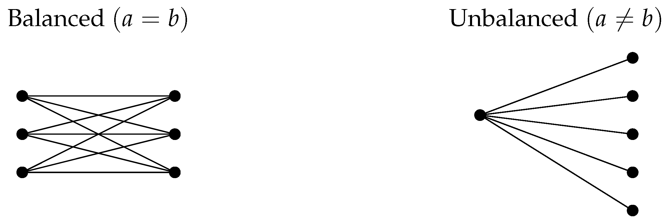
(see Figure 2).

Proof. 

(i) The case $d=2$ follows from the fact that ${\mathcal{B}}_n^2$ consists of complete bipartite graphs $K_{a,n-a}$ and the maximum is attained at $a=\lfloor n/2\rfloor$. For $d=3$, the extremal graph has the form $G[1·1,a,b,1·1]$ and, by Theorem 1, $|a-b|\le 1$, hence $G\cong G_{n,3}^{1,1}=G_{n,d}^{d-2,1}$.

(ii) For $d\in \{4,5,6\}$, the statement can be verified by calculations. Now assume $d\ge 7$.

• Case 1. $n-d=2k$ with $k\ge 1$. Then $\lfloor {\displaystyle \frac{n-d+1}{2}}\rfloor =k$, $\lceil {\displaystyle \frac{n-d+1}{2}}\rceil =k+1$ and

  $$\begin{array}{cc}\hfill DSO\left(G_{n,d}^{1,d-2}\right)& ={(k+1)}^2\gamma (k+1,k+2)+k\gamma (k,k+2)+\gamma (k+2,2)+\gamma (2,1)\hfill \\ \hfill & +(d-5)\gamma (2,2),\hfill \\ \hfill DSO\left(G_{n,d}^{2,d-3}\right)& =(k^2+3k+1)\gamma (k+1,k+2)+\gamma (k+2,2)+\gamma (k+1,1)+\gamma (2,1)\hfill \\ \hfill & +(d-6)\gamma (2,2),\hfill \\ \hfill DSO\left(G_{n,d}^{3,d-4}\right)& =\cdots =DSO\left(G_{n,d}^{d-4,3}\right)\hfill \\ \hfill & =(k^2+3k+1)\gamma (k+1,k+2)+\gamma (k+2,2)+\gamma (k+1,2)+2\gamma (2,1)\hfill \\ \hfill & +(d-7)\gamma (2,2),\hfill \\ \hfill DSO\left(G_{n,d}^{d-3,2}\right)& =(k^2+3k+1)\gamma (k+1,k+2)+\gamma (k+2,1)+\gamma (k+1,2)+\gamma (2,1)\hfill \\ \hfill & +(d-6)\gamma (2,2),\hfill \\ \hfill DSO\left(G_{n,d}^{d-2,1}\right)& =k(k+2)\gamma (k+1,k+2)+\sqrt{2}{(k+1)}^2+\gamma (k+1,2)+\gamma (2,1)\hfill \\ \hfill & +(d-5)\gamma (2,2).\hfill \end{array}$$

Since $\eta (x,y)=\gamma (x,y)-\gamma (x-1,y)$ and according Lemma 2, we obtain

$$DSO\left(G_{n,d}^{d-3,2}\right)-DSO\left(G_{n,d}^{2,d-3}\right)=\eta (k+2,1)-\eta (k+2,2)>0,$$

$$DSO\left(G_{n,d}^{d-3,2}\right)-DSO\left(G_{n,d}^{3,d-4}\right)=\eta (2,2)-\eta (2,k+2)>0,$$

$$\begin{array}{cc}\hfill DSO\left(G_{n,d}^{d-3,2}\right)-DSO\left(G_{n,d}^{d-2,1}\right)& =(k+1)[\gamma (k+1,k+2)-\sqrt{2}(k+1)]+\gamma (k+2,1)\hfill \\ \hfill & -\gamma (2,2)>0\hfill \end{array}$$

$$\begin{array}{cc}\hfill DSO\left(G_{n,d}^{d-3,2}\right)-DSO\left(G_{n,d}^{1,d-2}\right)& =k\left[\gamma \right(k+1,k+2)-\gamma (k,k+2\left)\right]\hfill \\ \hfill & -\left[\gamma \right(2,k+2)-\gamma (1,k+2\left)\right]+\left[\gamma \right(k+1,2)-\gamma (2,2\left)\right]\hfill \\ \hfill & \ge k\left[\eta \right(k+1,k+2)-\eta (2,k+2\left)\right]\hfill \\ \hfill & \ge \left[\eta \right(k+1,k+2)-\eta (2,k+2\left)\right]\ge 0.\hfill \end{array}$$

Thus $G_{n,d}^{d-3,2}$ attains the maximum when $n-d$ is even and $d\ge 7$.

• Case 2. $n-d=2k-1$ with $k\ge 1$.

Then $\lfloor {\displaystyle \frac{n-d+1}{2}}\rfloor =\lceil {\displaystyle \frac{n-d+1}{2}}\rceil =k$. If $k=1$, then $G\cong P_n$ and the statement is trivial. Assume $k\ge 2$.

Then,

$$\begin{array}{cc}\hfill DSO\left(G_{n,d}^{d-2,1}\right)& =(k^2+k)\gamma (k+1,k+1)+k\gamma (k,k+1)+\gamma (k+1,2)+\gamma (2,1)\hfill \\ \hfill & +(d-5)\gamma (2,2),\hfill \\ \hfill DSO\left(G_{n,d}^{d-3,2}\right)& =(k^2+2k)\gamma (k+1,k+1)+\gamma (k+1,2)+\gamma (k+1,1)+\gamma (2,1)\hfill \\ \hfill & +(d-6)\gamma (2,2),\hfill \\ \hfill DSO\left(G_{n,d}^{d-4,3}\right)& =\cdots =DSO\left(G_{n,d}^{3,d-4}\right)\hfill \\ \hfill & =(k^2+2k)\gamma (k+1,k+1)+2\gamma (k+1,2)+2\gamma (2,1)+(d-7)\gamma (2,2).\hfill \end{array}$$

Moreover,

$$\begin{array}{cc}\hfill DSO\left(G_{n,d}^{d-3,2}\right)-DSO\left(G_{n,d}^{d-2,1}\right)& =\left[\gamma (k+1,1)-\gamma (2,2)\right]+k\left[\gamma (k+1,k+1)-\gamma (k,k+1)\right]\hfill \\ \hfill & >\gamma (k+1,1)-\gamma (2,2)\ge \gamma (3,1)-\gamma (2,2)>0,\hfill \end{array}$$

and

$$DSO\left(G_{n,d}^{d-3,2}\right)-DSO\left(G_{n,d}^{d-4,3}\right)=\eta (2,2)-\eta (2,k+1)>0$$

according to Lemma 2 and $k\ge 2$. □

Remark 1.

The extremal graphs described in Theorem 2 exhibit a layered structure in which only two adjacent partition sets contain multiple vertices, while all other layers consist of a single vertex. This configuration reflects the balance condition established in Theorem 1 and highlights the role of diameter in shaping the global structure of graphs maximizing the diminished Sombor index.

3. Ordering the Extremal Maximum Graphs in ${\mathcal{B}}_{\mathit{n}}^{\mathit{d}}$ with Respect to Their Diameters

Let

$${\tau }_D\left(d\right)=\left\{\begin{array}{cc}DSO\left(G_{n,d}^{d-2,1}\right),\hfill & d=2,3,\hfill \\ DSO\left(G_{n,d}^{d-3,2}\right),\hfill & d\ge 4.\hfill \end{array}\right.$$

By Theorem 2, ${\tau }_D\left(d\right)$ is the maximal diminished Sombor index among all graphs in ${\mathcal{B}}_n^d$.

Theorem 3.

Let $2\le d\le n-1$. For fixed n, the function ${\tau }_D\left(d\right)$ is strictly decreasing in d.

Proof. 

We divide the proof into two claims.

Claim 2.

For $d\ge 6$,

$${\tau }_D(n-1)<{\tau }_D(n-2)<\cdots <{\tau }_D\left(7\right)<{\tau }_D\left(6\right).$$

Proof (Proof of Claim 2). 

We distinguish two cases according to the parity of $n-d$.

• Case A: $n-d=2k$ with $k\ge 1$.

Then $n-(d+1)=2k-1$ and

$$\begin{array}{cc}\hfill {\tau }_D\left(d\right)& =(k^2+3k+1)\gamma (k+1,k+2)+\gamma (k+2,1)+\gamma (k+1,2)+\gamma (2,1)+(d-6)\gamma (2,2),\hfill \\ \hfill {\tau }_D(d+1)& =(k^2+2k)\gamma (k+1,k+1)+\gamma (k+1,2)+\gamma (k+1,1)+\gamma (2,1)+(d-5)\gamma (2,2).\hfill \end{array}$$

Hence

$$\begin{array}{cc}\hfill {\tau }_D\left(d\right)-{\tau }_D(d+1)& =(k^2+2k)\left[\gamma (k+1,k+2)-\gamma (k+1,k+1)\right]\hfill \\ \hfill & +k\gamma (k+1,k+2)+\left[\gamma (k+2,1)-\gamma (k+1,1)\right]-\gamma (2,2).\hfill \end{array}$$

Since $\gamma (x,y)\ge {\displaystyle \frac{1}{\sqrt{2}}}$ with equality if and only if $x=y$, we have $\gamma (k+1,k+1)=\gamma (2,2)={\displaystyle \frac{\sqrt{2}}{2}}$,

$$\gamma (k+1,k+2)=\gamma (k+2,k+1)>\gamma (k+1,k+1).$$

and

$$\gamma (k+2,1)>\gamma (k+1,1).$$

Therefore,

$$k\gamma (k+1,k+2)-\gamma (2,2)>k{\displaystyle \frac{\sqrt{2}}{2}}-{\displaystyle \frac{\sqrt{2}}{2}}=(k-1){\displaystyle \frac{\sqrt{2}}{2}}\ge 0,$$

and ${\tau }_D\left(d\right)>{\tau }_D(d+1)$.

• Case B: $n-d=2k-1$ with $k\ge 2$.

Then $n-(d+1)=2(k-1)$ and

$$\begin{array}{cc}\hfill {\tau }_D\left(d\right)& =(k^2+2k)\gamma (k+1,k+1)+\gamma (k+1,2)+\gamma (k+1,1)+\gamma (2,1)+(d-6)\gamma (2,2),\hfill \\ \hfill {\tau }_D(d+1)& =(k^2+k-1)\gamma (k,k+1)+\gamma (k+1,1)+\gamma (k,2)+\gamma (2,1)+(d-5)\gamma (2,2).\hfill \end{array}$$

Thus

$$\begin{array}{cc}\hfill {\tau }_D\left(d\right)-{\tau }_D(d+1)& =(k^2+k-1)\left[\gamma (k+1,k+1)-\gamma (k,k+1)\right]\hfill \\ \hfill & +(k+1)\gamma (k+1,k+1)+\left[\gamma (k+1,2)-\gamma (k,2)\right]-\gamma (2,2).\hfill \end{array}$$

Since $\gamma (k+1,k+1)=\gamma (2,2)={\displaystyle \frac{\sqrt{2}}{2}}$, we obtain

$$(k+1)\gamma (k+1,k+1)-\gamma (2,2)=k{\displaystyle \frac{\sqrt{2}}{2}}>0.$$

Also, for $x>y$ (with $y=2$ and $k\ge 2$), $\gamma (k+1,2)-\gamma (k,2)>0$ and $\gamma (k+1,k+1)-\gamma (k,k+1)<0$. Writing

$$\gamma (k,k+1)={\displaystyle \frac{\sqrt{2k^2+2k+1}}{2k+1}}={\displaystyle \frac{1}{\sqrt{2}}}\sqrt{1+{\displaystyle \frac{1}{{(2k+1)}^2}}},$$

and using $\sqrt{1+t}\le 1+{\displaystyle \frac{t}{2}}$ for $t\ge 0$, we get

$$0<\gamma (k,k+1)-{\displaystyle \frac{1}{\sqrt{2}}}\le {\displaystyle \frac{1}{2\sqrt{2}}}{\displaystyle \frac{1}{{(2k+1)}^2}}.$$

Hence

$$(k^2+k-1)\left[\gamma (k+1,k+1)-\gamma (k,k+1)\right]\ge -{\displaystyle \frac{k^2+k-1}{2\sqrt{2}{(2k+1)}^2}}.$$

Since ${\displaystyle \frac{k^2+k-1}{{(2k+1)}^2}}<{\displaystyle \frac{1}{4}}$ for $k\ge 2$, it follows that

$$(k^2+k-1)\left[\gamma (k+1,k+1)-\gamma (k,k+1)\right]>-{\displaystyle \frac{1}{8\sqrt{2}}}.$$

Consequently,

$${\tau }_D\left(d\right)-{\tau }_D(d+1)>k{\displaystyle \frac{\sqrt{2}}{2}}-{\displaystyle \frac{1}{8\sqrt{2}}}>0,$$

and thus ${\tau }_D\left(d\right)>{\tau }_D(d+1)$ also in this case.

This completes the proof of Claim 2. □

Claim 3.

$${\tau }_D\left(6\right)<{\tau }_D\left(5\right)<{\tau }_D\left(4\right)<{\tau }_D\left(3\right)<{\tau }_D\left(2\right).$$

Proof (Proof of Claim 3). 

Assume first that $n=2n_0$ is even, where $n_0\ge 4$. Using the extremal structures for $2\le d\le 6$, we obtain

$$\begin{array}{cc}\hfill {\tau }_D\left(2\right)& =n_0^2\gamma (n_0,n_0),\hfill \\ \hfill {\tau }_D\left(3\right)& =2(n_0-1)\gamma (n_0,n_0-1)+{(n_0-1)}^2\gamma (n_0,n_0),\hfill \\ \hfill {\tau }_D\left(4\right)& ={(n_0-1)}^2\gamma (n_0,n_0-1)+(n_0-2)\gamma (n_0,n_0-2)+n_0\gamma (n_0,1),\hfill \\ \hfill {\tau }_D\left(5\right)& =2\gamma (n_0-1,1)+(n_0^2-2n_0)\gamma (n_0-1,n_0-1),\hfill \\ \hfill {\tau }_D\left(6\right)& =\gamma (n_0-1,1)+(n_0^2-3n_0+1)\gamma (n_0-1,n_0-2)+\gamma (n_0-2,2)+\gamma (2,1).\hfill \end{array}$$

Hence we have

$${\tau }_D\left(2\right)-{\tau }_D\left(3\right)=2(n_0-1)\left[\gamma (n_0,n_0)-\gamma (n_0,n_0-1)\right]+(2n_0-1)\gamma (n_0,n_0)>0$$

$$\begin{array}{cc}\hfill {\tau }_D\left(3\right)-{\tau }_D\left(4\right)& =2(n_0-1)\gamma (n_0,n_0-1)+{(n_0-1)}^2\gamma (n_0,n_0)\hfill \\ \hfill & -{(n_0-1)}^2\gamma (n_0,n_0-1)-(n_0-2)\gamma (n_0,n_0-2)-n_0\gamma (n_0,1)\hfill \\ \hfill & ={(n_0-1)}^2\left[\gamma (n_0,n_0)-\gamma (n_0,n_0-1)\right]\hfill \\ \hfill & +(n_0-2)\left[\gamma (n_0,n_0-1)-\gamma (n_0,n_0-2)\right]\hfill \\ \hfill & +n_0\left[\gamma (n_0,n_0-1)-\gamma (n_0,1)\right]>0\hfill \end{array}$$

$$\begin{array}{cc}\hfill {\tau }_D\left(4\right)-{\tau }_D\left(5\right)& ={(n_0-1)}^2\gamma (n_0,n_0-1)+(n_0-2)\gamma (n_0,n_0-2)+n_0\gamma (n_0,1)\hfill \\ \hfill & -2\gamma (n_0-1,1)-n_0(n_0-2)\gamma (n_0-1,n_0-1)\hfill \\ \hfill & =n_0(n_0-2)\left[\gamma (n_0,n_0-1)-\gamma (n_0-1,n_0-1)\right]\hfill \\ \hfill & +\left[\gamma (n_0,n_0-1)-\gamma (n_0-1,1)\right]+\left[\gamma (n_0,1)-\gamma (n_0-1,1)\right]\hfill \\ \hfill & +(n_0-2)\gamma (n_0,n_0-2)>0\hfill \end{array}$$

$$\begin{array}{cc}\hfill {\tau }_D\left(5\right)-{\tau }_D\left(6\right)& =\left[\gamma (n_0-1,1)-\gamma (2,1)\right]+(n_0^2-3n_0+1)[\gamma (n_0-1,n_0-1)\hfill \\ \hfill & -\gamma (n_0-1,n_0-2)]+(n_0-1)\left[\gamma (n_0-1,n_0-1)-\gamma (n_0-2,2)\right]>0.\hfill \end{array}$$

Thus ${\tau }_D\left(6\right)<{\tau }_D\left(5\right)<{\tau }_D\left(4\right)<{\tau }_D\left(3\right)<{\tau }_D\left(2\right)$ holds when n is even. The case when n is odd can be treated analogously. This completes the proof of Claim 3. □

According to Claims 2 and 3, ${\tau }_D\left(d\right)$ is strictly decreasing in d for fixed n. This completes the proof of the theorem. □

Corollary 1.

Among all connected bipartite graphs with fixed order n, the maximum diminished Sombor index is attained by the complete bipartite graph $K_{\lfloor n/2\rfloor ,\lceil n/2\rceil }$.

Theorem 4.

Let ${\mathcal{B}}_n$ be the set of all connected bipartite graphs with $n\ge 2$ vertices. For $G\in {\mathcal{B}}_n$, denote by $DSO{\left(G\right)}_{\max },DSO{\left(G\right)}_{\sec },DSO{\left(G\right)}_{\mathrm{thi}}$ and $DSO{\left(G\right)}_{\min }$ the largest, the second-largest, the third-largest and the smallest diminished Sombor index, respectively. Then:

(i) 

$DSO{\left(G\right)}_{\min }=DSO\left(P_n\right)$;

(ii) 

$DSO{\left(G\right)}_{\max }=DSO\left(K_{\lfloor n/2\rfloor ,\lceil n/2\rceil }\right)$;

(iii) 

$DSO{\left(G\right)}_{\sec }=DSO\left(K_{\lfloor (n-2)/2\rfloor ,\lceil (n+2)/2\rceil }\right)$ and $DSO{\left(G\right)}_{\mathrm{thi}}=DSO\left(G_{n,3}^{1,1}\right)$ for $n\ge 4$.

Proof. 

Parts (i) and (ii) follow from Theorem 3. For fixed n, the function ${\tau }_D\left(d\right)$ is strictly decreasing in d. Hence the maximal value is attained at $d=2$ and the minimal value at $d=n-1$. By Theorem 2, these values are attained by $K_{\lfloor n/2\rfloor ,\lceil n/2\rceil }$ and $P_n$, respectively.

We now prove (iii).

Let $G\in {\mathcal{B}}_n^2$. Since G is bipartite and $d=2$, every pair of vertices in different bipartition classes must be adjacent (otherwise their distance would be an odd number at least 3). Hence G is a complete bipartite graph $K_{a,n-a}$. For such graphs,

$$DSO\left(K_{a,n-a}\right)=a(n-a)\gamma (a,n-a),1\le a\le ⌊{\displaystyle \frac{n}{2}}⌋.$$

Define

$$f_D\left(x\right)=x(n-x)\gamma (x,n-x)={\displaystyle \frac{x(n-x)}{n}}\sqrt{x^2+{(n-x)}^2}.$$

A direct differentiation yields

$$f_D^{\prime }\left(x\right)={\displaystyle \frac{n-2x}{n}}{\displaystyle \frac{x^2+{(n-x)}^2-x(n-x)}{\sqrt{x^2+{(n-x)}^2}}}>0\left(1\le x<{\displaystyle \frac{n}{2}}\right),$$

since $x^2+{(n-x)}^2-x(n-x)=3{(x-{\displaystyle \frac{n}{2}})}^2+{\displaystyle \frac{n^2}{4}}>0$. Hence $f_D$ is strictly increasing on $[1,\lfloor n/2\rfloor ]$. Therefore $K_{\lfloor (n-2)/2\rfloor ,\lceil (n+2)/2\rceil }$ has the second-largest diminished Sombor index in ${\mathcal{B}}_n^2$.

By Theorem 2, $G_{n,3}^{1,1}$ attains the maximal diminished Sombor index in ${\mathcal{B}}_n^3$.

Since ${\tau }_D\left(d\right)$ is strictly decreasing in d, we have

$$max\{DSO\left(G\right):G\in {\mathcal{B}}_n^d\}<max\{DSO\left(G\right):G\in {\mathcal{B}}_n^3\}(d\ge 4).$$

Hence the second-largest value in ${\mathcal{B}}_n$ must come from either ${\mathcal{B}}_n^2$ or ${\mathcal{B}}_n^3$. Thus it suffices to compare

$$DSO\left(K_{\lfloor (n-2)/2\rfloor ,\lceil (n+2)/2\rceil }\right)\mathrm{and}DSO\left(G_{n,3}^{1,1}\right).$$

Odd $n\ge 5$. Write $n=2t+1$ with $t\ge 2$. Then

$$DSO\left(K_{t-1,t+2}\right)=(t-1)(t+2)\gamma (t-1,t+2).$$

Moreover, $G_{n,3}^{1,1}=G[1·1,t-1,t,1·1]$ and from the structure of $G_{n,3}^{1,1}$ we obtain

$$DSO\left(G_{n,3}^{1,1}\right)=(t-1)\gamma (t-1,t+1)+t(t-1)\gamma (t,t+1)+t\gamma (t,t).$$

Since $\gamma (t,t)={\displaystyle \frac{\sqrt{2}}{2}}$,

$$DSO\left(G_{n,3}^{1,1}\right)=(t-1)\gamma (t-1,t+1)+t(t-1)\gamma (t,t+1)+t{\displaystyle \frac{\sqrt{2}}{2}}.$$

Hence, we obtain

$$\begin{array}{cc}\hfill DSO\left(K_{t-1,t+2}\right)-DSO\left(G_{n,3}^{1,1}\right)& =t(t-1)\left[\gamma (t-1,t+2)-\gamma (t,t+1)\right]\hfill \\ \hfill & +(t-1)\left[2\gamma (t-1,t+2)-\gamma (t-1,t+1)\right]\hfill \\ \hfill & +t\left[\gamma (t-1,t+2)-{\displaystyle \frac{\sqrt{2}}{2}}\right].\hfill \end{array}$$

Each term is strictly positive: $\gamma (t-1,t+2)={\displaystyle \frac{\sqrt{2t^2+2t+5}}{2t+1}}>{\displaystyle \frac{\sqrt{2t^2+2t+1}}{2t+1}}=\gamma (t,t+1),$ $\gamma (t-1,t+2)>\gamma (t-1,t+1)$ and $\gamma (t-1,t+2)>{\displaystyle \frac{\sqrt{2}}{2}}$ since $\gamma (x,y)\ge {\displaystyle \frac{\sqrt{2}}{2}}$ with equality only at $x=y$. Hence $DSO\left(K_{t-1,t+2}\right)>DSO\left(G_{n,3}^{1,1}\right)$ for all odd $n\ge 5$.

• Even $n\ge 4$. Write $n=2n_0$ with $n_0\ge 2$. Then

$$DSO\left(K_{n_0-1,n_0+1}\right)=(n_0^2-1)\gamma (n_0-1,n_0+1),$$

where

$$\gamma (n_0-1,n_0+1)={\displaystyle \frac{\sqrt{{(n_0-1)}^2+{(n_0+1)}^2}}{2n_0}}={\displaystyle \frac{\sqrt{2n_0^2+2}}{2n_0}}.$$

Moreover, for $G_{n,3}^{1,1}=G[1·1,n_0-1,n_0-1,1·1]$, and from the structure of $G_{n,3}^{1,1}$ we obtain

$$DSO\left(G_{n,3}^{1,1}\right)=2(n_0-1)\gamma (n_0,n_0-1)+{(n_0-1)}^2\gamma (n_0,n_0),$$

where

$$\gamma (n_0,n_0-1)={\displaystyle \frac{\sqrt{n_0^2+{(n_0-1)}^2}}{2n_0-1}}={\displaystyle \frac{\sqrt{2n_0^2-2n_0+1}}{2n_0-1}},\gamma (n_0,n_0)={\displaystyle \frac{\sqrt{2}}{2}}.$$

Hence,

$$\begin{array}{cc}\hfill DSO\left(K_{n_0-1,n_0+1}\right)-DSO\left(G_{n,3}^{1,1}\right)& =(n_0^2-1)\gamma (n_0-1,n_0+1)-2(n_0-1)\gamma (n_0,n_0-1)\hfill \\ \hfill & -{(n_0-1)}^2{\displaystyle \frac{\sqrt{2}}{2}}\hfill \\ \hfill & =2(n_0-1)\left[(n_0+1)\gamma (n_0-1,n_0+1)-\gamma (n_0,n_0-1)\right]\hfill \\ \hfill & +{(n_0-1)}^2\left[\gamma (n_0-1,n_0+1)-{\displaystyle \frac{\sqrt{2}}{2}}\right]>0.\hfill \end{array}$$

Therefore $DSO\left(K_{n_0-1,n_0+1}\right)>DSO\left(G_{n,3}^{1,1}\right)$ for all even $n\ge 4$.

Combining the odd and even cases yields

$$DSO\left(K_{\lfloor (n-2)/2\rfloor ,\lceil (n+2)/2\rceil }\right)>DSO\left(G_{n,3}^{1,1}\right)(n\ge 4),$$

and hence

$$DSO{\left(G\right)}_{\sec }=DSO\left(K_{\lfloor (n-2)/2\rfloor ,\lceil (n+2)/2\rceil }\right).$$

The third-largest value in $B_n^2$ is attained at

$$K_{\lfloor (n-4)/2\rfloor ,\lceil (n+4)/2\rceil }.$$

It remains to show that

$$DSO\left(G_{n,3}^{1,1}\right)>DSO\left(K_{\lfloor (n-4)/2\rfloor ,\lceil (n+4)/2\rceil }\right).$$

Even $n=2n_0$, $n_0\ge 3$. Then $G_{n,3}^{1,1}$ has $m_G=n_0^2-1$ edges, hence

$$DSO\left(G_{n,3}^{1,1}\right)\ge m_G{\displaystyle \frac{\sqrt{2}}{2}}.$$

On the other hand, $K_{n_0-2,n_0+2}$ has $m_K=n_0^2-4$ edges and $\gamma (x,y)<1$, so

$$DSO\left(K_{n_0-2,n_0+2}\right)<m_K.$$

Since $(n_0^2-1){\displaystyle \frac{\sqrt{2}}{2}}>n_0^2-4$ for $n_0\ge 3$, we obtain $DSO\left(G_{n,3}^{1,1}\right)>DSO\left(K_{n_0-2,n_0+2}\right)$ for even $n\ge 6$.

• Odd $n=2n_0+1$, $n_0\ge 3$. Then $G_{n,3}^{1,1}$ has $m_G=n_0^2+n_0-1$ edges, hence

$$DSO\left(G_{n,3}^{1,1}\right)\ge m_G{\displaystyle \frac{\sqrt{2}}{2}}.$$

Also $K_{n_0-2,n_0+3}$ has $m_K=n_0^2+n_0-6$ edges, so

$$DSO\left(K_{n_0-2,n_0+3}\right)<m_K.$$

Since $(n_0^2+n_0-1){\displaystyle \frac{\sqrt{2}}{2}}>n_0^2+n_0-6$ for $n_0\ge 3$, we get $DSO\left(G_{n,3}^{1,1}\right)>DSO\left(K_{n_0-2,n_0+3}\right)$ for odd $n\ge 7$. The remaining small cases $n=4,5,6$ can be verified by direct computation. Therefore,

$$DSO{\left(G\right)}_{\mathrm{thi}}=DSO\left(G_{n,3}^{1,1}\right)(n\ge 4).$$

This completes the proof. □

Example 1.

To illustrate the conclusions of Theorems 2 and 4 concretely, we compute the explicit DSO values and identify the corresponding extremal structures for small values of n.

• Case $\mathit{n}=\mathbf{6}$.   The extremal graph is $K_{3,3}$ (diameter $d=2$). Its vertices in each partition class have degree 3, so

  $$DSO\left(K_{3,3}\right)=9{\displaystyle \frac{\sqrt{3^2+3^2}}{3+3}}=9{\displaystyle \frac{3\sqrt{2}}{6}}={\displaystyle \frac{9\sqrt{2}}{2}}\approx 6.364.$$
  The second-extremal graph is $K_{2,4}$ (diameter $d=2$):

  $$DSO\left(K_{2,4}\right)=8{\displaystyle \frac{\sqrt{2^2+4^2}}{2+4}}=8{\displaystyle \frac{\sqrt{20}}{6}}={\displaystyle \frac{4\sqrt{20}}{3}}\approx 5.963.$$
  The third-extremal graph is $G_{6,3}^{1,1}=G[1·1,2,2,1·1]$ (diameter $d=3$):

  $$DSO\left(G_{6,3}^{1,1}\right)=4{\displaystyle \frac{\sqrt{2^2+3^2}}{2+3}}+4{\displaystyle \frac{\sqrt{3^2+2^2}}{3+2}}=8{\displaystyle \frac{\sqrt{13}}{5}}\approx 5.771.$$
• Case $\mathit{n}=\mathbf{7}$.  The extremal graph is $K_{3,4}$ (diameter $d=2$):

  $$DSO\left(K_{3,4}\right)=12{\displaystyle \frac{\sqrt{3^2+4^2}}{3+4}}=12{\displaystyle \frac{5}{7}}={\displaystyle \frac{60}{7}}\approx 8.571.$$
  The second-extremal graph is $K_{2,5}$ (diameter $d=2$):

  $$DSO\left(K_{2,5}\right)=10{\displaystyle \frac{\sqrt{2^2+5^2}}{2+5}}=10{\displaystyle \frac{\sqrt{29}}{7}}\approx 7.690.$$
  The third-extremal graph is $G_{7,3}^{1,1}=G[1·1,2,3,1·1]$ (diameter $d=3$):

  $$DSO\left(G_{7,3}^{1,1}\right)=2{\displaystyle \frac{\sqrt{2^2+4^2}}{2+4}}+6{\displaystyle \frac{\sqrt{4^2+3^2}}{4+3}}+3{\displaystyle \frac{\sqrt{3^2+4^2}}{3+4}}={\displaystyle \frac{\sqrt{20}}{3}}+{\displaystyle \frac{30}{7}}+{\displaystyle \frac{15}{7}}\approx 7.403.$$
  These examples confirm the ordering $DS{O}_{\max }>DS{O}_{\sec }>DS{O}_{\mathrm{thi}}$ established in Theorem 4, and illustrate how the index value decreases as the diameter increases from 2 to 3.

The results obtained above provide a coherent structural understanding of the diminished Sombor index in bipartite graphs. Theorem 1 establishes a fundamental balance condition, showing that extremal configurations require adjacent partition sizes to differ by at most one. This result highlights the importance of degree balance in maximizing the total contribution of the index.

Building on this, Theorem 2 characterizes the precise structure of extremal graphs, revealing that they possess a layered configuration in which only two consecutive partition sets may contain multiple vertices, while all other layers consist of a single vertex. This provides a complete description of the graphs attaining the maximal DSO value.

Theorem 3 further clarifies the role of global graph structure by proving that the maximal diminished Sombor index is strictly decreasing with respect to the diameter. This demonstrates that more compact graphs yield higher index values, whereas increasing distances between vertices reduce the overall contribution.

Finally, Theorem 4 complements these results by establishing a complete ordering of bipartite graphs with respect to their DSO values, identifying the graphs that attain the largest, second-largest, and third-largest indices.

Taken together, these results show that the diminished Sombor index is governed by a delicate interplay between local degree balance and global distance constraints, providing a unified perspective on its extremal behavior.

4. Discussion

In this paper, we studied the diminished Sombor index of connected bipartite graphs of fixed order and diameter. The main contribution of the paper is the complete determination of the sharp upper bound of the diminished Sombor index in the class ${\mathcal{B}}_n^d$, together with the characterization of all extremal graphs attaining this bound. Our results show that, despite the normalized form of the diminished Sombor index, the extremal structures exhibit a strong rigidity phenomenon. More precisely, once the distance partition is considered, the maximizing graph must have at most two consecutive nontrivial partition sets, and these two layers must be as balanced as possible. This balancing property plays a central role in the proof and eventually leads to the complete identification of the extremal graphs in ${\mathcal{B}}_n^d$.

Another important outcome of the paper is the strict monotonicity of the extremal value with respect to the diameter. This shows that, for fixed order n, the maximal diminished Sombor index decreases as the diameter increases. Consequently, the extremal graphs can also be ordered according to their diameters, which makes it possible to determine the connected bipartite graphs with the largest, second-largest, third-largest, and smallest diminished Sombor indices.

The methods used here rely essentially on edge transfer arguments, distance–partition analysis, and careful comparisons of the local contributions of the function $\gamma (x,y)={\displaystyle \frac{\sqrt{x^2+y^2}}{x+y}}$. These techniques may be useful in the study of other normalized Sombor-type indices or related degree-based graph invariants.

The present work focuses on classical combinatorial graphs; however, it is both natural and meaningful to ask whether the results can be extended to two-scale fractal spaces. The two-scale fractal dimension provides a geometric framework that captures the self-similar and non-self-similar structure of complex networks at different scales [33,34]. In fractal graph theory, the underlying metric structure is richer than in classical graphs: vertices may be organized according to fractal hierarchies rather than simple diameter-based layers, and the notion of distance is replaced by a more nuanced fractal distance.

Extending the extremal theory of the diminished Sombor index to such fractal graph structures represents a promising and important direction for future research. In particular, one could investigate whether the balance conditions and monotonicity properties established here have natural fractal analogues, and whether the layered extremal structures characterized in Theorem 2 correspond to self-similar configurations in fractal networks. Such an extension would bridge discrete graph theory and fractal geometry, potentially offering new tools for the structural analysis of complex molecular and biological networks.

There are several directions for further research. A natural open problem is to determine the minimum diminished Sombor index among bipartite graphs with fixed order n and diameter d, since in the present paper only the maximal case is completely resolved.

It would also be interesting to investigate extremal values of the diminished Sombor index for bipartite graphs under other graph parameters, such as matching number, connectivity, domination number, or girth.

Beyond classical graph families, extending the analysis to fractal graph models, including Sierpiński-type graphs and hierarchical networks arising in chemistry and biology, represents a particularly promising direction. The interplay between fractal dimension and degree-based indices in such settings is largely unexplored [33,34].

Moreover, the results of this paper provide a foundation for applying the diminished Sombor index in quantitative structure–property relationship (QSPR) modeling, particularly for bipartite molecular graphs such as those arising in coordination chemistry and polymer science. Correlating the extremal DSO values with physicochemical properties of molecules would be a natural applied counterpart to the theoretical results established here.

Finally, another natural direction is to investigate the relationship between the DSO index and the cyclomatic number $\ell =m-n+1$ for bipartite graphs, which may provide additional structural insight beyond the diameter-based approach adopted in this work.

References

1. Bondy, J.A.; Murty, U.S.R. Graph Theory; Springer: New York, NY, USA, 2008. [Google Scholar]
2. Gutman, I. Degree-based topological indices. Croat. Chem. Acta 2013, 86, 351–361. [Google Scholar] [CrossRef] [Scilit]
3. Gutman, I. Geometric approach to degree-based topological indices: Sombor indices. MATCH Commun. Math. Comput. Chem. 2021, 86, 11–16. [Google Scholar]
4. Liu, H.; Gutman, I.; You, L.; Huang, Y. Sombor index: Review of extremal results and bounds. J. Math. Chem. 2022, 60, 771–798. [Google Scholar] [CrossRef] [Scilit]
5. Movahedi, F.; Akhbari, M.H. Degree-based topological indices of the molecular structure of hyaluronic acid–methotrexate conjugates in cancer treatment. Int. J. Quantum Chem. 2023, 123, e27106. [Google Scholar] [CrossRef] [Scilit]
6. Zhou, T.; Lin, Z.; Miao, L. The Sombor index of trees and unicyclic graphs with given maximum degree. Discret. Math. Lett. 2021, 7, 24–29. [Google Scholar] [CrossRef] [Scilit]
7. Movahedi, F.; Akhbari, M.H. Entire Sombor index of graphs. Iran. J. Math. Chem. 2023, 14, 33–45. [Google Scholar]
8. Liu, H.; Chen, H.; Xiao, Q.; Fang, X.; Tang, Z. More on Sombor indices of chemical graphs and their applications to the boiling point of benzenoid hydrocarbons. Int. J. Quantum Chem. 2021, 121, e26689. [Google Scholar] [CrossRef] [Scilit]
9. Movahedi, F.; Zameni, M.; Akhbari, M.H.; Shahavi, M.H.; Rajabnezhad, S. Topological indices and data analysis techniques modeling to predict the physicochemical properties of tetracycline antibiotics. J. Pharm. Sci. 2025, 114, 103871. [Google Scholar] [CrossRef] [Scilit] [PubMed]
10. Samiei, Z.; Movahedi, F. Investigating graph invariants for predicting properties of chemical structures of antiviral drugs. Polycycl. Aromat. Compd. 2023, 44, 6696–6713. [Google Scholar] [CrossRef] [Scilit]
11. Rajathagiri, D.T. Enhanced mathematical models for the Sombor index: Reduced and co-Sombor index perspectives. Data Anal. Artif. Intell. 2021, 1, 215–228. [Google Scholar]
12. Movahedi, F.; Gutman, I.; Redžepović, I.; Furtula, B. Diminished Sombor index. MATCH Commun. Math. Comput. Chem. 2026, 95, 141–162. [Google Scholar] [CrossRef] [Scilit]
13. Movahedi, F. Maximal Diminished Sombor index of tricyclic graphs. MATCH Commun. Math. Comput. Chem. 2025; in press. [CrossRef] [Scilit]
14. Das, K.C.; Harshini, R.; Elumalai, S. Resolving the conjecture of tricyclic graphs minimizing the Diminished Sombor index. MATCH Commun. Math. Comput. Chem. 2026, 95, 935–939. [Google Scholar] [CrossRef] [Scilit]
15. Movahedi, F. Diminished Sombor index and its relationship with topological indices. Filomat 2025, 39, 10519–10532. [Google Scholar]
16. Cruz, R.; Rada, J. Extremal values of the Sombor index in unicyclic and bicyclic graphs. J. Math. Chem. 2021, 59, 1098–1116. [Google Scholar] [CrossRef] [Scilit]
17. Cruz, R.; Gutman, I.; Rada, J. Sombor index of chemical graphs. Appl. Math. Comput. 2021, 399, 126018. [Google Scholar] [CrossRef] [Scilit]
18. Das, K.C.; Gutman, I. On Sombor index of trees. Appl. Math. Comput. 2022, 412, 126575. [Google Scholar] [CrossRef] [Scilit]
19. Liu, H. Extremal problems on Sombor indices of unicyclic graphs with a given diameter. Comput. Appl. Math. 2022, 41, 138. [Google Scholar] [CrossRef] [Scilit]
20. Sun, X.; Du, J. On Sombor index of trees with fixed domination number. Appl. Math. Comput. 2022, 421, 126946. [Google Scholar] [CrossRef] [Scilit]
21. Khanra, B.; Das, S. Euler Sombor index of trees, unicyclic and chemical graphs. MATCH Commun. Math. Comput. Chem. 2025, 94, 525–548. [Google Scholar] [CrossRef] [Scilit]
22. Kizilirmak, G.O. Extremal Euler Sombor index of unicyclic graphs with fixed diameter. MATCH Commun. Math. Comput. Chem. 2025, 94, 725–738. [Google Scholar] [CrossRef] [Scilit]
23. Ali, A.; Sekar, S.; Balachandran, S.; Elumalai, S.; Alanazi, A.M.; Hassan, T.S.; Shang, Y. Graphical edge-weight-function indices of trees. AIMS Math. 2024, 9, 32552–32570. [Google Scholar] [CrossRef] [Scilit]
24. Tache, A.P.; Tache, R.M.; Stroe, I. Extremal unicyclic graphs for the Euler Sombor index. MATCH Commun. Math. Comput. Chem. 2025, 94, 561–578. [Google Scholar] [CrossRef] [Scilit]
25. Hu, Y.; Fang, J.; Liu, Y.; Lin, Z. Bounds on the Euler Sombor index of maximal outerplanar graphs. Electron. J. Math. 2024, 8, 39–47. [Google Scholar] [CrossRef] [Scilit]
26. Kizilirmak, G.O. On Euler Sombor index of tricyclic graphs. MATCH Commun. Math. Comput. Chem. 2025, 94, 247–262. [Google Scholar] [CrossRef] [Scilit]
27. Ren, X.; Cao, G.; Wang, F.; Zhou, M. The Euler Sombor index of trees. MATCH Commun. Math. Comput. Chem. 2025, 94, 739–760. [Google Scholar] [CrossRef] [Scilit]
28. Zhang, Q.; Tchier, F.; Hussain, Z.; Aslam, A.; Zuo, X. On the bounds for the Euler Sombor index of molecular trees and its applications. J. Appl. Math. Comput. 2025, 71, 645–663. [Google Scholar] [CrossRef] [Scilit]
29. Albalahi, A.M.; Alanazi, A.M.; Alotaibi, A.M.; Hamza, A.E.; Ali, A. Optimizing the Euler Sombor index of (molecular) tricyclic graphs. MATCH Commun. Math. Comput. Chem. 2025, 94, 549–560. [Google Scholar] [CrossRef] [Scilit]
30. Su, Z.; Tang, Z. Extremal unicyclic graphs for the Euler Sombor index: Applications to benzenoid hydrocarbons and drug molecules. Axioms 2025, 14, 249. [Google Scholar] [CrossRef] [Scilit]
31. Das, K.C.; Bera, J. Resolving open problems on the Euler Sombor index. arXiv 2025, arXiv:2507.17246. [Google Scholar] [CrossRef] [Scilit]
32. Das, P.; Mondal, S.; Pal, A. Extremal Trees for Euler Sombor Index with Given Parameters. Available online: https://ssrn.com/abstract=5153080 (accessed on 25 February 2025).
33. Ain, Q.T.; He, J.-H. On two-scale dimension and its applications. Therm. Sci. 2019, 23, 1707–1712. [Google Scholar] [CrossRef] [Scilit]
34. He, J.-H.; Ain, Q.T. New promises and future challenges of fractal calculus: From two-scale thermodynamics to fractal variational principle. Therm. Sci. 2020, 24, 659–681. [Google Scholar] [CrossRef] [Scilit]
35. Zhai, M.; Liu, R.; Shu, J. On the spectral radius of bipartite graphs with given diameter. Linear Algebra Appl. 2009, 430, 1165–1170. [Google Scholar] [CrossRef] [Scilit]
Figure 1. A schematic layered representation of a bipartite graph in B n d with distance partition T 0 , T 1 , , T d . Each T i is an independent set, and edges occur only between consecutive layers. In the extremal configuration, only two adjacent layers ( T p and T p + 1 ) may contain multiple vertices, forming a complete bipartite subgraph, while the remaining layers consist of a single vertex.
Mathematics 14 01688 g001
Figure 2. Illustration of balanced and unbalanced partitions between adjacent layers. Balanced configurations maximize the number of edges between layers, while unbalanced configurations reduce edge density and overall DSO contribution.
Mathematics 14 01688 g002