First-Order Approximate Solutions for Nonlinear Smooth-Discontinuous (SD) Oscillator via Spreading Residue Harmonic Balance and Multiple Scales Methods

Abstract

This study presents a numerical and analytical investigation of the nonlinear smooth-discontinuous (SD) oscillator. The nonlinear restoring force is approximated by a fifth-order polynomial using a Taylor series expansion to simplify the governing equation while preserving the essential nonlinear characteristics of the system. To analyze the oscillator dynamics, two analytical approaches are applied, namely the spreading residue harmonic balance method (SRHPM) and the Multiple Scales Method (MSM). The obtained analytical solutions are validated through comparison with numerical simulations carried out using the classical fourth-order Runge–Kutta scheme. The results reveal a strong agreement between the analytical and numerical solutions, confirming the capability of both SRHPM and MSM to accurately describe the nonlinear oscillatory response of the SD system.

1. Introduction

Nonlinear phenomena are present across virtually every field of physics and engineering, shaping the behavior of systems that span from micro-scale devices to large-scale structural frameworks [1,2,3,4,5,6,7,8,9,10]. Among these, strongly nonlinear oscillators pose a distinct analytical challenge, as their governing equations rarely yield closed-form solutions. Although numerical methods can deliver highly accurate results, analytical and semi-analytical approaches remain essential for revealing the underlying dynamics, enabling fast performance predictions, and informing practical design choices. Oscillators, by definition, are dynamical systems that exhibit periodic motion, repeating particular patterns or states over time [11].

Of particular interest is the smooth-discontinuous (SD) oscillator, which has drawn significant attention in recent decades for its exceptional ability to achieve low- and ultra-low-frequency vibration isolation [12,13]. Characterized by hybrid smooth-discontinuous behavior [14], the SD oscillator typically comprises an elastic beam resembling a snap-through truss, along with a mass, inclined elastic springs, and a rigid support. Given its importance in vibration control, various control strategies have been applied to this oscillator. For example, Abd El-Salam et al. [15,16] examined proportional (P), derivative (D), proportional–derivative (PD), and negative derivative feedback controllers for both smooth and discontinuous oscillators, demonstrating their effectiveness in suppressing vibrations, enhancing stability, and improving performance in nonlinear and discontinuous regimes. Over recent decades, a wide range of perturbation and analytical methods has been developed for solving nonlinear differential equations. Numerical approaches typically rely on time-stepping integration of the governing equations from arbitrary initial conditions until steady-state responses are achieved [17]. Approximation methods, in contrast, often assume steady-state behavior from the outset and employ Fourier series expansions to determine system responses [18,19,20,21]. Despite their usefulness, these methods can suffer from drawbacks such as high computational cost or limited long-term validity. To address these challenges, analytical techniques including the harmonic balance method [22,23] and Li–He’s modified homotopic perturbation method [24] have been proposed. For instance, Junfeng [25] applied the global residue harmonic balance method to a strongly nonlinear oscillator with cubic and harmonic restoring forces, while Qian et al. [26] extended the spreading residue harmonic balance method to obtain second-order approximate solutions for doubly clamped beam-type N/MEMS resonators. Liu et al. [27] presented a comprehensive review on the nonlinear dynamics and vibration behavior of lightweight composite structures, highlighting recent developments in analytical, numerical, and experimental approaches. Their study discussed major nonlinear phenomena and outlined current challenges associated with modeling accuracy, material complexity, and dynamic stability in advanced composite systems. Among the available perturbation techniques, the Multiple Scale Method (MSM) stands out as a powerful and versatile approach for analyzing nonlinear dynamical systems. Its main advantage lies in producing uniformly valid approximate analytical solutions over extended time intervals, thereby eliminating secular terms and divergences common in conventional perturbation expansions. By introducing multiple independent time scales, MSM effectively separates fast and slow dynamics, offering deep insights into the interplay among different frequency components, resonance effects, and amplitude–phase modulation. This capability makes MSM particularly well-suited for oscillator and vibration problems, where the combined effects of nonlinearity, damping, and external excitation give rise to complex behaviors that are difficult to capture through numerical simulations alone. Consequently, MSM not only advances theoretical understanding but also provides a practical framework for performance prediction and robust control design, and has been widely applied in oscillator and vibration studies [28,29,30,31,32].

This paper investigates the dynamics of the smooth-discontinuous (SD) oscillator. The remainder of the paper is organized as follows. Section 2 presents the mathematical formulation of the SD oscillator model. Section 3 develops the analytical solutions of the governing equation using the spreading residue harmonic balance method (SRHBM) and the Method of Multiple Scales (MSM), including the derivation of first-order approximate solutions. Section 4 provides numerical simulations and discusses the corresponding phase portraits and time-history responses, together with comparisons to numerical solutions obtained using the fourth-order Runge–Kutta method. Finally, the main conclusions and remarks are summarized in Section 5.

2. Mathematical Model

The mechanical model examined in this work is a simplified mass–spring system, inspired by the first vibrational mode of an elastic arch [33,34] and analogous to a snap-through truss.

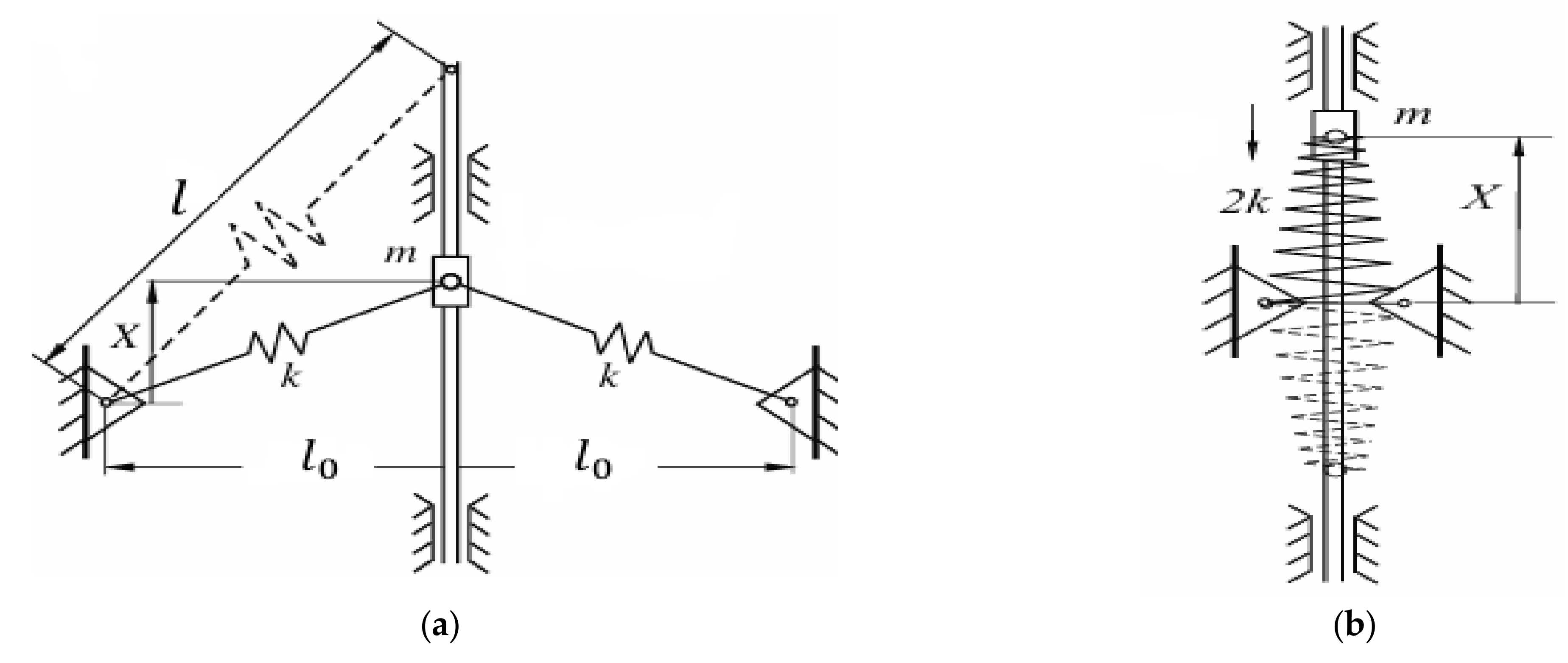
As shown in Figure 1a, it comprises a lumped mass $m$ connected to a rigid frame by two linearly elastic springs, each with stiffness $k$ and equilibrium length $l$, capable of carrying both tensile and compressive loads. Although the springs exhibit linear elastic behavior, the vertical restoring force transmitted to the mass is inherently nonlinear due to the system’s geometric arrangement. For simplicity and without loss of generality, the system mass was normalized by taking a mass $m=1$, and all governing equations were derived in nondimensional form. The potential energy $V\left(X\right)$ as follows:

$$V(X)=k\left({\displaystyle \frac{X^2}{2}}-l\sqrt{X^2+l_0}\right)$$

(1)

Differentiate the potential energy with respect to $x$.

$${\displaystyle \frac{dV}{dX}}=k\left(X-{\displaystyle \frac{l\hspace{0.17em}X}{\sqrt{X^2+l_0^2}}}\right)$$

(2)

Using Lagrange’s principle, we can define the Lagrangian for this system as:

$$L={\displaystyle \frac{1}{2}}{\dot{X}}^2-V(X)$$

(3)

According to Lagrange’s formulation,

$${\displaystyle \frac{d}{dt}}\left({\displaystyle \frac{\partial L}{\partial \dot{X}}}\right)-\left({\displaystyle \frac{\partial L}{\partial X}}\right)=0$$

(4)

Applying Lagrange’s equation allows us to derive the equation of motion as follows:

$$\left.\begin{array}{l}\ddot{X}+{\displaystyle \frac{dV}{dX}}=0\\ \ddot{X}+k\left(X-{\displaystyle \frac{l\hspace{0.17em}X}{\sqrt{X^2+l_0^2}}}\right)=0\end{array}\right\}$$

(5)

In this model, $l$ is the natural length of each spring, $X$ is the displacement of the unit-mass, and $l_0$ is half the distance between the rigid supports. Equation (5) can be nondimensionalized by defining $x={\displaystyle \frac{X}{l}}$ and $\alpha ={\displaystyle \frac{l_0}{l}}>0 \mathrm{a}\mathrm{s}$:

$$\ddot{x}+k\hspace{0.17em}x\left(1-{\displaystyle \frac{1}{\sqrt{x^2+{\alpha }^2}}}\right)=0$$

(6)

The geometrical parameter $\alpha$ governs the oscillator’s dynamic regime (Figure 1a). For $\propto >0$, the system behaves as a discrete elastic string, exhibiting smooth oscillations, whereas $\propto =0$ reduces it to a mass suspended by two parallel springs (Figure 1b), producing discontinuous dynamics. As $\alpha \to 0$, the transition from smooth to discontinuous motion is captured by the modified form of Equation (6). By decreasing the smoothness parameter $\alpha \to 0$. Equation (6) is now written as the following [35].

$$\ddot{x}+k\hspace{0.17em}\left(x-sign(x)\right)=0,\hspace{0.17em}\hspace{0.17em}\hspace{0.17em}\hspace{0.17em}\hspace{0.17em}\hspace{0.17em}sign(x)=\left\{\begin{array}{l}1,\hspace{0.17em}\hspace{0.17em}\hspace{0.17em}\hspace{0.17em}\hspace{0.17em}\hspace{0.17em}\hspace{0.17em}\hspace{0.17em}\hspace{0.17em}\hspace{0.17em}x>0\\ 0\hspace{0.17em}\hspace{0.17em}\hspace{0.17em}\hspace{0.17em}\hspace{0.17em}\hspace{0.17em}\hspace{0.17em}\hspace{0.17em}\hspace{0.17em}\hspace{0.17em}\hspace{0.17em}\hspace{0.17em}x=0\\ -1\hspace{0.17em}\hspace{0.17em}\hspace{0.17em}\hspace{0.17em}\hspace{0.17em}\hspace{0.17em}\hspace{0.17em}\hspace{0.17em}\hspace{0.17em}\hspace{0.17em}x<0\end{array}\right.$$

(7)

The approximation of the nonlinear Equation (6) is made tractable by employing a Taylor series representation of ${\displaystyle \frac{1}{\sqrt{x^2+{\alpha }^2}}}$ expressed as:

$${\displaystyle \frac{1}{\sqrt{x^2+{\alpha }^2}}}\approx {\displaystyle \frac{1}{\alpha }}-{\displaystyle \frac{x^2}{2{\alpha }^3}}+{\displaystyle \frac{9x^4}{24{\alpha }^5}}-\cdot \cdot \cdot$$

(8)

So, the approximated form of Equation (6) can be given by:

$$\ddot{x}+{\displaystyle \frac{k\hspace{0.17em}(\alpha -1)}{\alpha }}x+{\displaystyle \frac{k}{2{\alpha }^3}}{x}^3-{\displaystyle \frac{9k}{24{\alpha }^5}}{x}^5=0,\hspace{0.17em}\hspace{0.17em}\hspace{0.17em}\hspace{0.17em}\hspace{0.17em}\hspace{0.17em}\hspace{0.17em}\hspace{0.17em}\hspace{0.17em}\hspace{0.17em}\hspace{0.17em}\hspace{0.17em}\hspace{0.17em}x(0)=A,\hspace{0.17em}\hspace{0.17em}\dot{x}(0)=0$$

(9)

To obtain an approximate solution of Equation (9), the spreading residue harmonic balance method (SRHBM) and the Multiple Scale Method (MSM), with first-order approximate solutions, will be employed. Its results will then be compared with the numerical solution obtained using the Runge–Kutta method.

3. Approximate Solution

3.1. Spreading Residue Harmonic Balance Method

The concept of the SRHBM involves distributing the residual error obtained after substituting an approximate solution into the governing equation across the entire period. The SRHBM technique promotes a more uniform reduction of the residual over the whole domain, enhancing convergence and solution stability. To apply the SRHBM method to obtain the solution of Equation (9), we introduce a transformation of the time as $\mathit{\tau }=\mathit{\omega }\mathit{t}$; therefore, Equation (9) can be written as:

$${\omega }^2{x}^{″}+{\displaystyle \frac{k\hspace{0.17em}(\alpha -1)}{\alpha }}x+{\displaystyle \frac{k}{2{\alpha }^3}}{x}^3-{\displaystyle \frac{9k}{24{\alpha }^5}}{x}^5=0$$

(10)

Here, ${(.)}^{\mathit{\prime }}$ denotes differentiation with respect to $\mathit{\tau }$, and $\mathit{\omega }$ refers to the angular frequency. Since Equation (10) admits a periodic solution, it can be expressed [36] as:

$$x_j(\tau )={\displaystyle \sum _{i=1}^j{a}_{2i+1,j}\left\{\cos (\tau )-\cos \left((2i+1)\tau \right)\right\}}$$

(11)

According to the initial conditions in Equation (9), the zeroth-order approximation can be written as:

$$x_0(\tau )=A\cos \left(\tau \right),\hspace{0.17em}\hspace{0.17em}\hspace{0.17em}\hspace{0.17em}\tau ={\omega }_{0}t$$

(12)

Based on the homotopy approach, a parameter $\mathit{p}\in \left[\mathbf{0,1}\right]$ is introduced. The steady-state solution, together with its associated angular frequency, is expressed as [37]:

$$x(\tau )=x_0(\tau )+p\hspace{0.17em}{x}_1(\tau )+\cdot \cdot \cdot$$

(13)

$${\omega }^2={\omega }_0^2+p{\omega }_1+\cdot \cdot \cdot$$

(14)

By inserting Equations (13) and (14) in Equation (10), this yields:

$$\left({\omega }_0^2{x^{″}}_0+{\displaystyle \frac{k\hspace{0.17em}(\alpha -1)}{\alpha }}{x}_0+{\displaystyle \frac{k}{2{\alpha }^3}}{x}_0^3-{\displaystyle \frac{9k}{24{\alpha }^5}}{x}_0^5\right)+p\left({\omega }_0^2{x^{″}}_1+{\omega }_1{x^{″}}_0+{\displaystyle \frac{k\hspace{0.17em}(\alpha -1)}{\alpha }}{x}_1+{\displaystyle \frac{3k}{2{\alpha }^3}}{x}_0^2{x}_1-{\displaystyle \frac{45k}{24{\alpha }^5}}{x}_0^4{x}_1\right)=0$$

(15)

3.1.1. The Zeroth-Level Approximation

To derive the zeroth-order approximation, Equation (12) is substituted into Equation (15), after which the coefficients $p^0$ are collected. This process yields the harmonic residue in the form:

$$\begin{array}{l}{R}_0(\tau )={\omega }_0^2{x^{″}}_0+{\displaystyle \frac{k\hspace{0.17em}(\alpha -1)}{\alpha }}{x}_0+{\displaystyle \frac{k}{2{\alpha }^3}}{x}_0^3-{\displaystyle \frac{9k}{24{\alpha }^5}}{x}_0^5\\ \hspace{0.17em}\hspace{0.17em}\hspace{0.17em}\hspace{0.17em}\hspace{0.17em}\hspace{0.17em}\hspace{0.17em}\hspace{0.17em}\hspace{0.17em}\hspace{0.17em}\hspace{0.17em}\hspace{0.17em}\hspace{0.17em}=\left(-{\omega }_0^{2}A+{\displaystyle \frac{k\hspace{0.17em}(\alpha -1)}{\alpha }}A+{\displaystyle \frac{3k}{8{\alpha }^3}}{A}^3-{\displaystyle \frac{45k}{192{\alpha }^5}}{A}^5\right)\cos (\tau )+\left({\displaystyle \frac{k}{8{\alpha }^3}}{A}^3-{\displaystyle \frac{45k}{384{\alpha }^5}}{A}^5\right)\cos (3\tau )\\ \hspace{0.17em}\hspace{0.17em}\hspace{0.17em}\hspace{0.17em}\hspace{0.17em}\hspace{0.17em}\hspace{0.17em}\hspace{0.17em}\hspace{0.17em}\hspace{0.17em}\hspace{0.17em}\hspace{0.17em}\hspace{0.17em}-\left({\displaystyle \frac{9k}{384{\alpha }^5}}{A}^5\right)\cos (5\tau )\end{array}$$

(16)

In accordance with the Galerkin procedure [38], Equation (16) should be free of the secular term $\mathrm{c}\mathrm{o}\mathrm{s}\left(\tau \right)$. By imposing that its coefficient vanishes, we will obtain:

$$-{\omega }_0^{2}A+{\displaystyle \frac{k\hspace{0.17em}(\alpha -1)}{\alpha }}A+{\displaystyle \frac{3k}{8{\alpha }^3}}{A}^3-{\displaystyle \frac{45k}{192{\alpha }^5}}{A}^5=0$$

(17)

Thus, the approximated frequency ${\omega }_0$ is given by:

$${\omega }_0=\sqrt{{\displaystyle \frac{192k\hspace{0.17em}({\alpha }^5-{\alpha }^4)+72k\hspace{0.17em}{\alpha }^2{A}^2-45k\hspace{0.17em}{A}^4}{192{\alpha }^5}}}$$

(18)

The zero-approximation solution can be written as:

$$x_0(t)=A\cos \left(\sqrt{{\displaystyle \frac{192k\hspace{0.17em}({\alpha }^5-{\alpha }^4)+72k\hspace{0.17em}{\alpha }^2{A}^2-45k\hspace{0.17em}{A}^4}{192{\alpha }^5}}}t\right)$$

(19)

3.1.2. The First Approximation

To evaluate the first approximation, the coefficient of $p^1$ is collected as:

$${\psi }_1(\tau )={\omega }_0^2{x^{″}}_1+{\omega }_1{x^{″}}_0+{\displaystyle \frac{k\hspace{0.17em}(\alpha -1)}{\alpha }}{x}_1+{\displaystyle \frac{3k}{2{\alpha }^3}}{x}_0^2{x}_1-{\displaystyle \frac{45k}{24{\alpha }^5}}{x}_0^4{x}_1$$

(20)

Equation (20) is linear with respect to ${\omega }_1$ and $x_1\left(\tau \right)$. According to Equation (11), if we put $j=1$, the first approximation solution takes the following form:

$$x_1(\tau )=a_{3,1}\left\{\cos \left(\tau \right)-\cos \left(3\tau \right)\right\}$$

(21)

where $a_{\mathrm{3,1}}$ is unknown to be determined. Substituting from Equations (12) and (21) to evaluate ${ \psi }_1\left(\tau \right)$. For convenience, we denote the harmonic residue of this approximation as:

$${\mathrm{R}}_1(\tau )={\psi }_1(\tau )+{\mathrm{R}}_0(\tau )$$

(22)

Equation (22) can be evaluated as follows:

$$\begin{array}{l}{R}_1(\tau )=\left(\begin{array}{l}-{\omega }_0^2{a}_{3,1}+{\displaystyle \frac{k\hspace{0.17em}(\alpha -1)}{\alpha }}{a}_{3,1}+{\displaystyle \frac{3k\hspace{0.17em}{A}^2}{4\hspace{0.17em}{\alpha }^3}}{a}_{3,1}-{\displaystyle \frac{135k\hspace{0.17em}{A}^4}{96\hspace{0.17em}{\alpha }^5}}{a}_{3,1}-{\omega }_{1}A-{\omega }_0^{2}A\\ +{\displaystyle \frac{k\hspace{0.17em}(\alpha -1)}{\alpha }}A+{\displaystyle \frac{3k\hspace{0.17em}{A}^3}{8\hspace{0.17em}{\alpha }^3}}-{\displaystyle \frac{45k\hspace{0.17em}{A}^5}{192\hspace{0.17em}{\alpha }^5}}\end{array}\right)\cos (\tau )\\ \hspace{0.17em}\hspace{0.17em}\hspace{0.17em}\hspace{0.17em}\hspace{0.17em}\hspace{0.17em}\hspace{0.17em}\hspace{0.17em}\hspace{0.17em}\hspace{0.17em}\hspace{0.17em}\hspace{0.17em}\hspace{0.17em}+\left(9{\omega }_0^2{a}_{3,1}-{\displaystyle \frac{k\hspace{0.17em}(\alpha -1)}{\alpha }}{a}_{3,1}-{\displaystyle \frac{3k\hspace{0.17em}{A}^2}{4\hspace{0.17em}{\alpha }^3}}{a}_{3,1}+{\displaystyle \frac{45k\hspace{0.17em}{A}^4}{224\hspace{0.17em}{\alpha }^5}}{a}_{3,1}+{\displaystyle \frac{3k\hspace{0.17em}{A}^3}{8\hspace{0.17em}{\alpha }^3}}-{\displaystyle \frac{45k\hspace{0.17em}{A}^5}{384\hspace{0.17em}{\alpha }^5}}\right)\cos (3\tau )\\ \hspace{0.17em}\hspace{0.17em}\hspace{0.17em}\hspace{0.17em}\hspace{0.17em}\hspace{0.17em}\hspace{0.17em}\hspace{0.17em}\hspace{0.17em}\hspace{0.17em}\hspace{0.17em}\hspace{0.17em}\hspace{0.17em}-\left({\displaystyle \frac{3k\hspace{0.17em}{A}^2}{8\hspace{0.17em}{\alpha }^3}}{a}_{3,1}-{\displaystyle \frac{135k\hspace{0.17em}{A}^4}{96\hspace{0.17em}{\alpha }^5}}{a}_{3,1}+{\displaystyle \frac{9k\hspace{0.17em}{A}^5}{384\hspace{0.17em}{\alpha }^5}}\right)\cos (5\tau )+\left({\displaystyle \frac{45k\hspace{0.17em}{A}^4}{224\hspace{0.17em}{\alpha }^5}}{a}_{3,1}\right)\cos (7\tau )\end{array}$$

(23)

The unknown parameters ${\omega }_1$ and $a_{\mathrm{3,1}}$ in Equation (23) are obtained by equating the coefficients of $\mathrm{c}\mathrm{o}\mathrm{s}\left(\tau \right)$ and $\mathrm{c}\mathrm{o}\mathrm{s}\left(3\tau \right)$ to zero, yielding the two equations below.

$$-{\omega }_0^2{a}_{3,1}+{\displaystyle \frac{k\hspace{0.17em}(\alpha -1)}{\alpha }}{a}_{3,1}+{\displaystyle \frac{3k\hspace{0.17em}{A}^2}{4{\alpha }^3}}{a}_{3,1}-{\displaystyle \frac{135k\hspace{0.17em}{A}^4}{96{\alpha }^5}}{a}_{3,1}-{\omega }_{1}A-{\omega }_0^{2}A+{\displaystyle \frac{k\hspace{0.17em}(\alpha -1)}{\alpha }}A+{\displaystyle \frac{3k\hspace{0.17em}{A}^3}{8{\alpha }^3}}-{\displaystyle \frac{45k\hspace{0.17em}{A}^5}{192{\alpha }^5}}=0$$

(24)

$$9{\omega }_0^2{a}_{3,1}-{\displaystyle \frac{k\hspace{0.17em}(\alpha -1)}{\alpha }}{a}_{3,1}-{\displaystyle \frac{3k\hspace{0.17em}{A}^2}{4{\alpha }^3}}{a}_{3,1}+{\displaystyle \frac{45k\hspace{0.17em}{A}^4}{224{\alpha }^5}}{a}_{3,1}+{\displaystyle \frac{3k\hspace{0.17em}{A}^3}{8{\alpha }^3}}-{\displaystyle \frac{45k\hspace{0.17em}{A}^5}{384{\alpha }^5}}=0$$

(25)

From Equation (25), we can evaluate $a_{\mathrm{3,1}}$ after substituting from Equation (18) as:

$$a_{3,1}={\displaystyle \frac{5040A^5-16128{\alpha }^2{A}^3}{344064{\alpha }^4(\alpha -1)+89271{\alpha }^2{A}^2-82080A^4}}$$

(26)

It is easy to obtain ${\omega }_1$ from Equation (24) with the help of Equations (18) and (26) as follows:

$${\omega }_1={\displaystyle \frac{\left(72{\alpha }^2\gamma A-22572A^3\right)\left(5040A^5-16128{\alpha }^2{A}^3\right)}{192{\alpha }^5\left(344064{\alpha }^4(\alpha -1)+89271{\alpha }^2{A}^2-82080A^4\right)}}$$

(27)

As $p\to 1$, Equations (13) and (14) yield the first-order approximation solution and its corresponding frequency as:

$$\left\{\begin{array}{l}{x}_{(1)}(\tau )=x_{(0)}(\tau )+x_1(\tau )=\left(A+a_{3,1}\right)\cos (\tau )-a_{3,1}\cos (3\tau )\\ {\omega }_{(1)}=\sqrt{{\omega }_0^2+{\omega }_1}\end{array}\right.,\hspace{0.17em}\hspace{0.17em}\hspace{0.17em}\hspace{0.17em}\hspace{0.17em}\tau ={\omega }_{(1)}t$$

(28)

Therefore, the final form of the first-order approximation solution takes the following form:

$$\begin{array}{l}{x}_{(1)}(\tau )=\left(A+{\displaystyle \frac{5040\hspace{0.17em}{A}^5-16128\hspace{0.17em}{\alpha }^2{A}^3}{344064\hspace{0.17em}{\alpha }^4(\alpha -1)+89271\hspace{0.17em}{\alpha }^2{A}^2-82080\hspace{0.17em}{A}^4}}\right)\cos (\tau )\\ \hspace{0.17em}\hspace{0.17em}\hspace{0.17em}\hspace{0.17em}\hspace{0.17em}\hspace{0.17em}\hspace{0.17em}\hspace{0.17em}\hspace{0.17em}\hspace{0.17em}\hspace{0.17em}\hspace{0.17em}\hspace{0.17em}\hspace{0.17em}-\left({\displaystyle \frac{5040\hspace{0.17em}{A}^5-16128\hspace{0.17em}{\alpha }^2{A}^3}{344064\hspace{0.17em}{\alpha }^4(\alpha -1)+89271\hspace{0.17em}{\alpha }^2{A}^2-82080\hspace{0.17em}{A}^4}}\right)\cos (3\tau )\end{array}$$

(29)

$${\omega }_{(1)}=\sqrt{{\displaystyle \frac{192k\hspace{0.17em}({\alpha }^5-{\alpha }^4)+72k\hspace{0.17em}{\alpha }^2{A}^2-45k\hspace{0.17em}{A}^4}{192{\alpha }^5}}+{\displaystyle \frac{\left(72{\alpha }^2\gamma A-22572A^3\right)\left(5040A^5-16128{\alpha }^2{A}^3\right)}{192{\alpha }^5\left(344064{\alpha }^4(\alpha -1)+89271{\alpha }^2{A}^2-82080A^4\right)}}}$$

(30)

3.2. Multiple Scale Method

To obtain the solution of Equation (10) using the method of multiple scales, the equation is rewritten as follows:

$$\ddot{x}+{\sigma }^{2}x+{\Gamma }_1{x}^3-{\Gamma }_2{x}^5=0,\hspace{0.17em}\hspace{0.17em}\hspace{0.17em}\hspace{0.17em}\hspace{0.17em}\hspace{0.17em}\hspace{0.17em}\hspace{0.17em}\hspace{0.17em}\hspace{0.17em}\hspace{0.17em}\hspace{0.17em}\hspace{0.17em}x(0)=A,\hspace{0.17em}\hspace{0.17em}\dot{x}(0)=0$$

(31)

where the natural frequency:

$$\sigma =\sqrt{{\displaystyle \frac{k\hspace{0.17em}(\alpha -1)}{\alpha }}}\mathrm{and} {\Gamma }_1={\displaystyle \frac{k}{2{\alpha }^3}},{\Gamma }_2={\displaystyle \frac{9k}{24{\alpha }^5}}$$

(32)

Based on the perturbation method, the first-order approximate solution for Equation (31) can be given by [39].

$$x(t,\epsilon )=x_0(T_0,T_1)+\epsilon x_1(T_0,T_1)+\cdot \cdot \cdot$$

(33)

where $\epsilon$ is the perturbation parameter with values in the interval [0, 1], $T_0=t$, and $T_1=\epsilon t$.

According to the time scales $T_0$, and $T_1$, the derivatives ${\displaystyle \frac{d}{dt}}$ and ${\displaystyle \frac{d^2}{{dt}^2}}$ can be expressed as [40]:

$$\left\{\begin{array}{l}{\displaystyle \frac{d}{dt}}=D_0+\epsilon D_1+\cdot \cdot \cdot \\ {\displaystyle \frac{d^2}{d{t}^2}}=D_0^2+2\epsilon D_0{D}_1+\cdot \cdot \cdot ,\hspace{0.17em}{D}_i={\displaystyle \frac{\partial }{\partial T_i}};i=0,1\end{array}\right.$$

(34)

For the purpose analysis, the system parameters are scaled as follows:

$${\Gamma }_1=\epsilon \hspace{0.17em}{\stackrel{⌢}{\Gamma }}_1,{\Gamma }_2=\epsilon \hspace{0.17em}{\stackrel{⌢}{\Gamma }}_2$$

(35)

Inserting Equations (32)–(35) into Equation (31) and then equating the coefficients that have the same power of $\epsilon$.

$$\left(D_0^2+{\sigma }^2\right)x_0=0,\hspace{0.17em}\hspace{0.17em}\hspace{0.17em}\hspace{0.17em}\hspace{0.17em}\hspace{0.17em}\hspace{0.17em}\hspace{0.17em}\hspace{0.17em}\hspace{0.17em}\hspace{0.17em}\hspace{0.17em}\hspace{0.17em}{x}_0(0)=A,\hspace{0.17em}{\dot{x}}_0(0)=0$$

(36)

$$\left(D_0^2+{\sigma }^2\right)x_1=-2D_0{D}_1{x}_0-{\stackrel{⌢}{\Gamma }}_1{x}_0^3+{\stackrel{⌢}{\Gamma }}_2{x}_0^5,\hspace{0.17em}\hspace{0.17em}\hspace{0.17em}\hspace{0.17em}\hspace{0.17em}\hspace{0.17em}\hspace{0.17em}\hspace{0.17em}\hspace{0.17em}\hspace{0.17em}\hspace{0.17em}\hspace{0.17em}\hspace{0.17em}{x}_1(0)=0,\hspace{0.17em}{\dot{x}}_1(0)=0$$

(37)

Equation (36), being a homogenous second-order differential equation, admits a solution of the form.

$$x_0\left(T_0,T_1\right)=c\left(T_1\right)\hspace{0.17em}{e}^{i\sigma T_0}+\overline{c}\left(T_1\right)\hspace{0.17em}{e}^{-i\sigma T_0}$$

(38)

where $i=\sqrt{-1}$, and the unknown function $c\left(T_1\right)$ will be calculated using the initial conditions.

According to the initial conditions in Equation (36), $c\left(T_1\right)=\overline{c}\left(T_1\right)={\displaystyle \frac{A}{2}}$. Therefore, the zero-approximation solution can be written as:

$$x_0\left(T_0,T_1\right)={\displaystyle \frac{A}{2}}\hspace{0.17em}{e}^{i\sigma T_0}+{\displaystyle \frac{A}{2}}\hspace{0.17em}{e}^{-i\sigma T_0}$$

(39)

We can simplify Equation (39) as:

$$x_0(t)=A\hspace{0.17em}\cos (\sigma \hspace{0.17em}t);\hspace{0.17em}\hspace{0.17em}\sigma =\sqrt{{\displaystyle \frac{k\hspace{0.17em}(\alpha -1)}{\alpha }}}$$

(40)

Inserting Equation (39) into the right-hand side of Equation (38) as follows:

$$\begin{array}{l}\left(D_0^2+{\sigma }^2\right)x_1=\left({\displaystyle \frac{10{\stackrel{⌢}{\Gamma }}_2{A}^5-12{\stackrel{⌢}{\Gamma }}_1{A}^3}{32}}\right)e^{i\sigma }+\left({\displaystyle \frac{10{\stackrel{⌢}{\Gamma }}_2{A}^5-12{\stackrel{⌢}{\Gamma }}_1{A}^3}{32}}\right)e^{-i\sigma }+\left({\displaystyle \frac{5{\stackrel{⌢}{\Gamma }}_2{A}^5-4{\stackrel{⌢}{\Gamma }}_1{A}^3}{32}}\right)e^{3i\sigma }+\left({\displaystyle \frac{5{\stackrel{⌢}{\Gamma }}_2{A}^5-4{\stackrel{⌢}{\Gamma }}_1{A}^3}{32}}\right)e^{-3i\sigma }\\ \hspace{0.17em}\hspace{0.17em}\hspace{0.17em}\hspace{0.17em}\hspace{0.17em}\hspace{0.17em}\hspace{0.17em}\hspace{0.17em}\hspace{0.17em}\hspace{0.17em}\hspace{0.17em}\hspace{0.17em}\hspace{0.17em}\hspace{0.17em}\hspace{0.17em}\hspace{0.17em}\hspace{0.17em}\hspace{0.17em}\hspace{0.17em}\hspace{0.17em}\hspace{0.17em}\hspace{0.17em}\hspace{0.17em}\hspace{0.17em}\hspace{0.17em}\hspace{0.17em}\hspace{0.17em}+\left({\displaystyle \frac{{\stackrel{⌢}{\Gamma }}_2{A}^5}{32}}\right)e^{5i\sigma }+\left({\displaystyle \frac{{\stackrel{⌢}{\Gamma }}_2{A}^5}{32}}\right)e^{-5i\sigma }\end{array}$$

(41)

To get the first approximation, we must eliminate all the secular terms from the right-hand side of Equation (41) by equating the coefficients of $e^{i\sigma }$ and $e^{-i\sigma }$ to zero. Therefore, the first approximation can be expressed as:

$$x_1(t)=\left({\displaystyle \frac{A^3\left(4{\stackrel{⌢}{\Gamma }}_1-5{\stackrel{⌢}{\Gamma }}_2{A}^2\right)}{256\hspace{0.17em}{\sigma }^2}}\right)e^{3i\sigma t}+\left({\displaystyle \frac{A^3\left(4{\stackrel{⌢}{\Gamma }}_1-5{\stackrel{⌢}{\Gamma }}_2{A}^2\right)}{256\hspace{0.17em}{\sigma }^2}}\right)e^{-3i\sigma t}-\left({\displaystyle \frac{{\stackrel{⌢}{\Gamma }}_2{A}^5}{768\hspace{0.17em}{\sigma }^2}}\right)e^{5i\sigma t}-\left({\displaystyle \frac{{\stackrel{⌢}{\Gamma }}_2{A}^5}{768\hspace{0.17em}{\sigma }^2}}\right)e^{-5i\sigma t}$$

(42)

We can simplify Equation (42) as:

$$x_1(t)=\left({\displaystyle \frac{4{\stackrel{⌢}{\Gamma }}_1{A}^3-5{\stackrel{⌢}{\Gamma }}_2{A}^5}{128\hspace{0.17em}{\sigma }^2}}\right)\hspace{0.17em}\cos (3\sigma t)-\left({\displaystyle \frac{{\stackrel{⌢}{\Gamma }}_2{A}^5}{384\hspace{0.17em}{\sigma }^2}}\right)\hspace{0.17em}\cos (5\sigma t)$$

(43)

In Equation (33) for $\epsilon \to 1$, the first-order approximation solution is written as:

$$x(t)=A\hspace{0.17em}\cos (\sigma t)+\left({\displaystyle \frac{4{\Gamma }_1{A}^3-5{\Gamma }_2{A}^5}{128\hspace{0.17em}{\sigma }^2}}\right)\hspace{0.17em}\cos (3\sigma t)-\left({\displaystyle \frac{{\Gamma }_2{A}^5}{384\hspace{0.17em}{\sigma }^2}}\right)\hspace{0.17em}\cos (5\sigma t)$$

(44)

4. Numerical Results

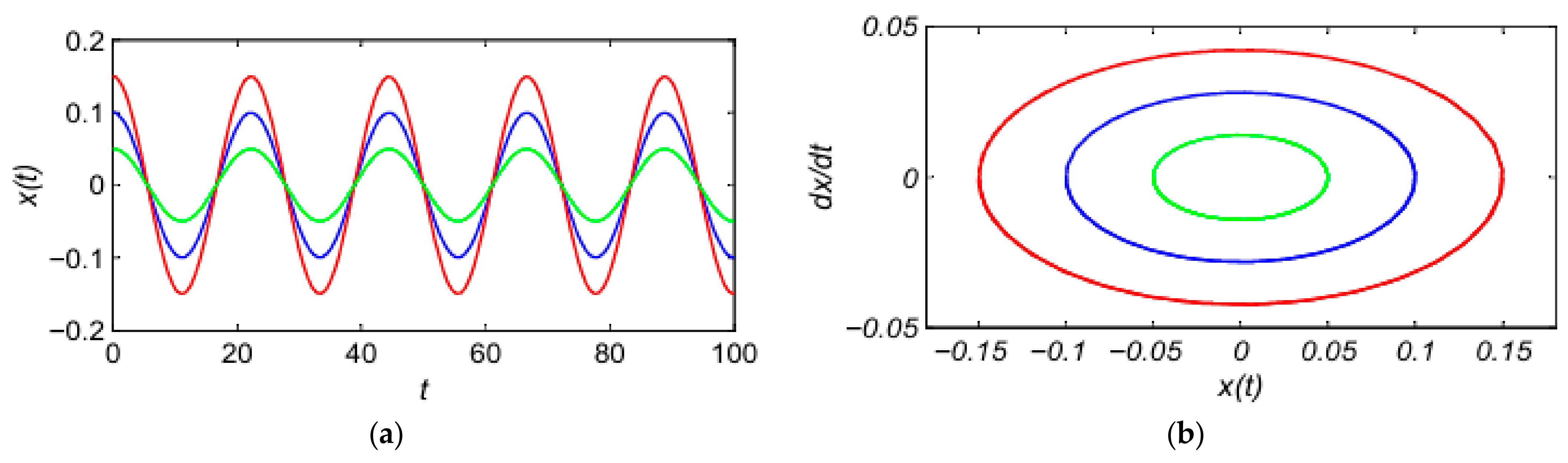
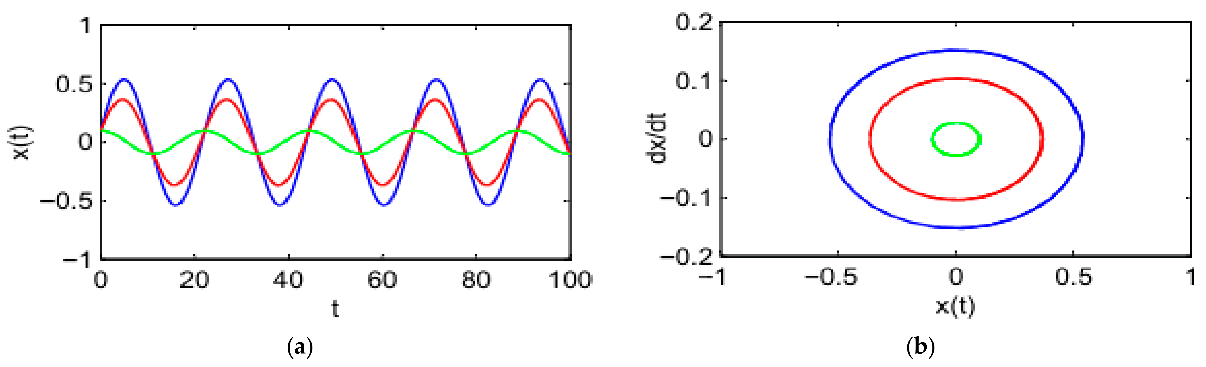
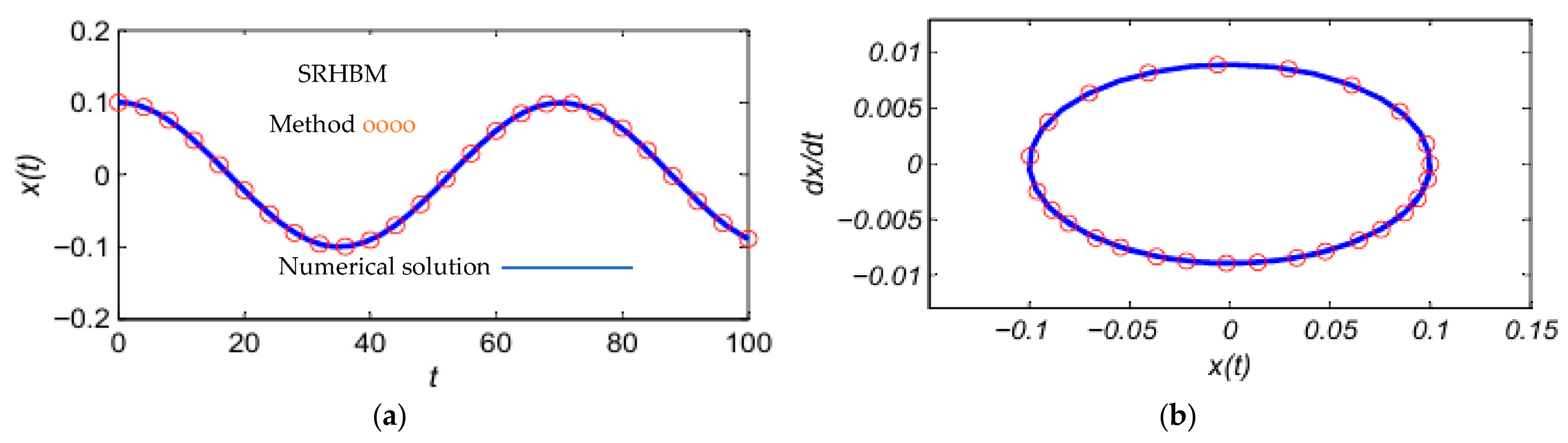
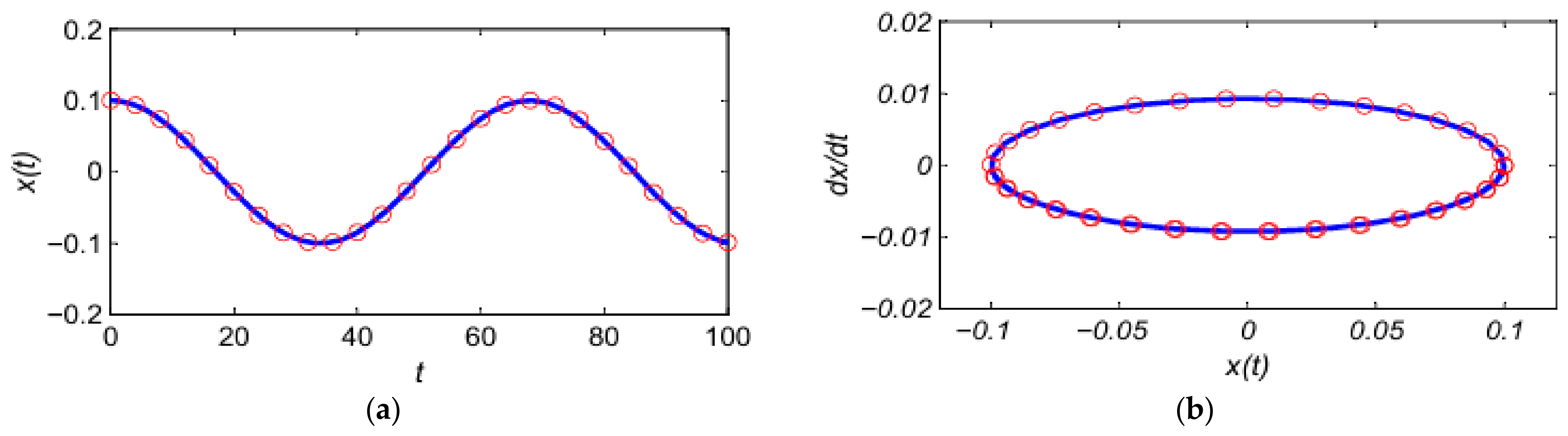
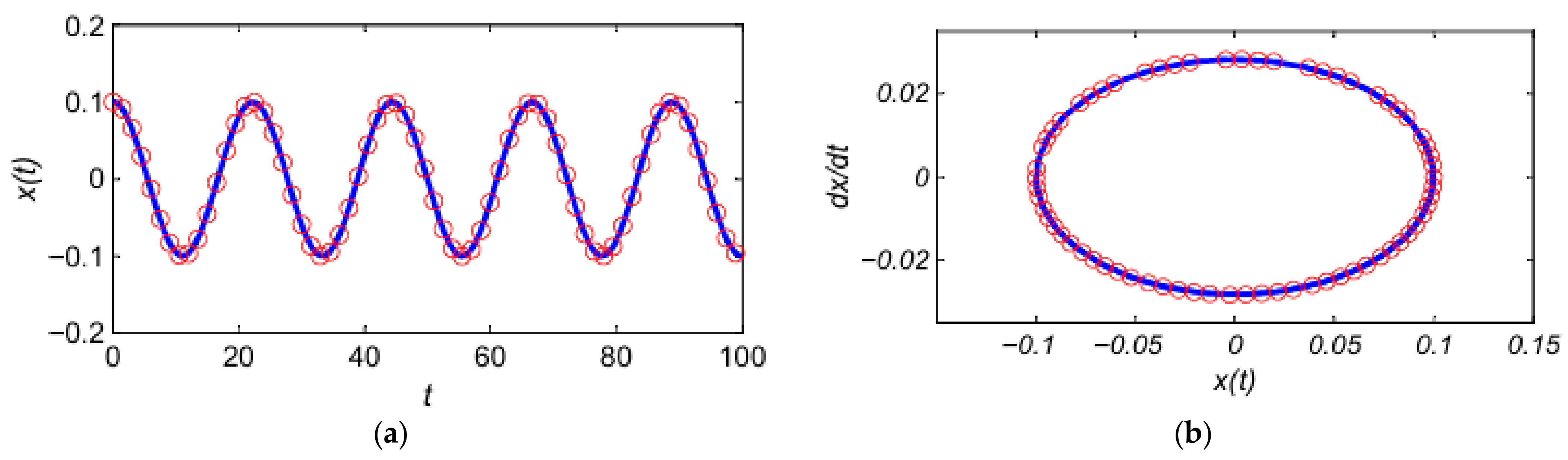
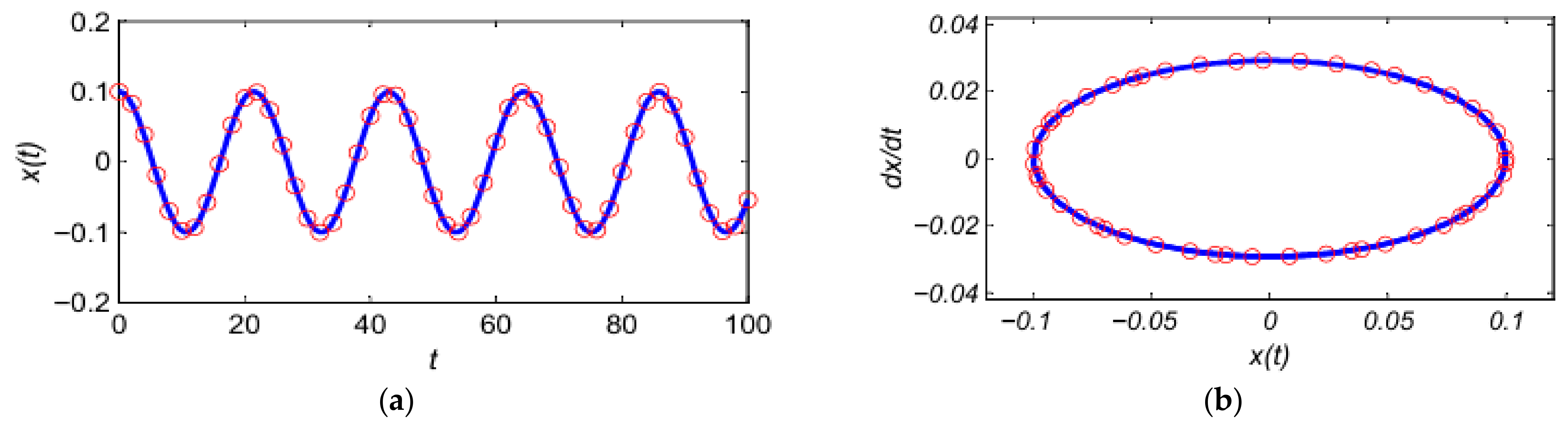
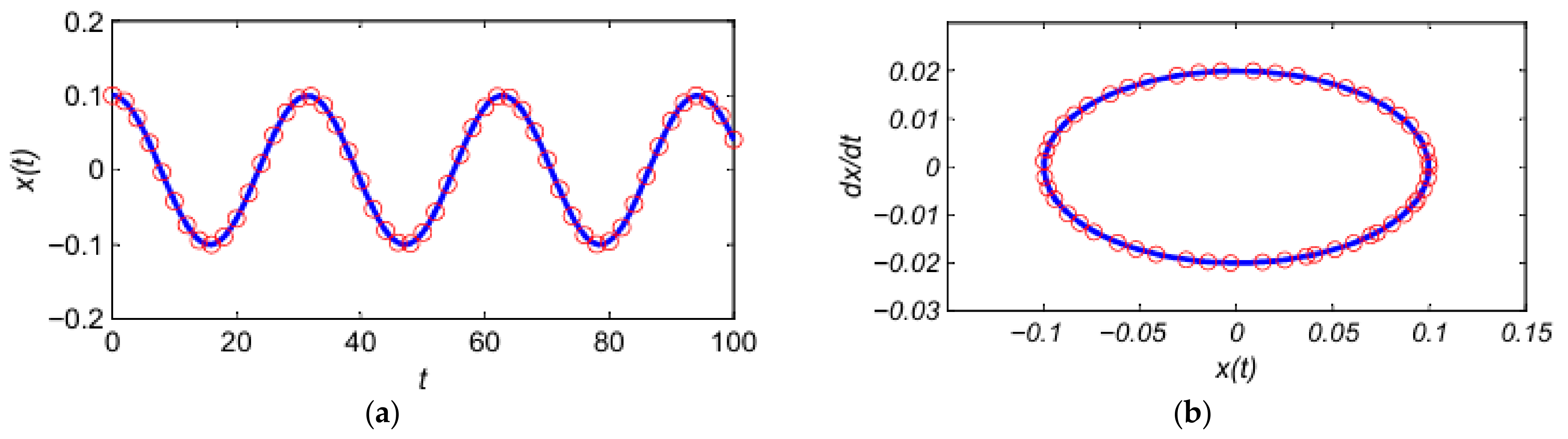
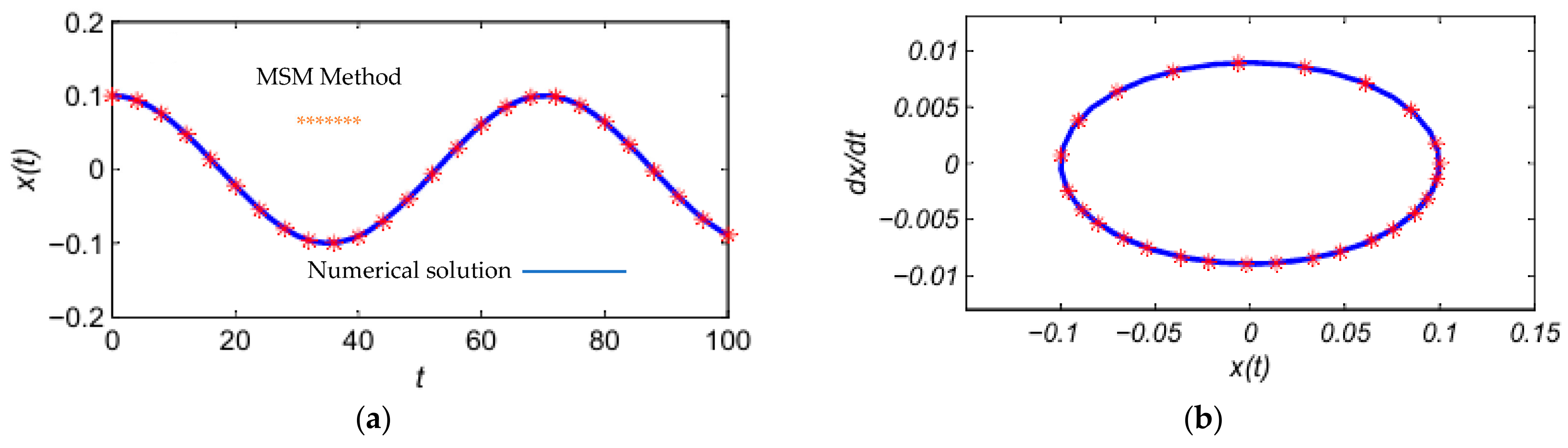
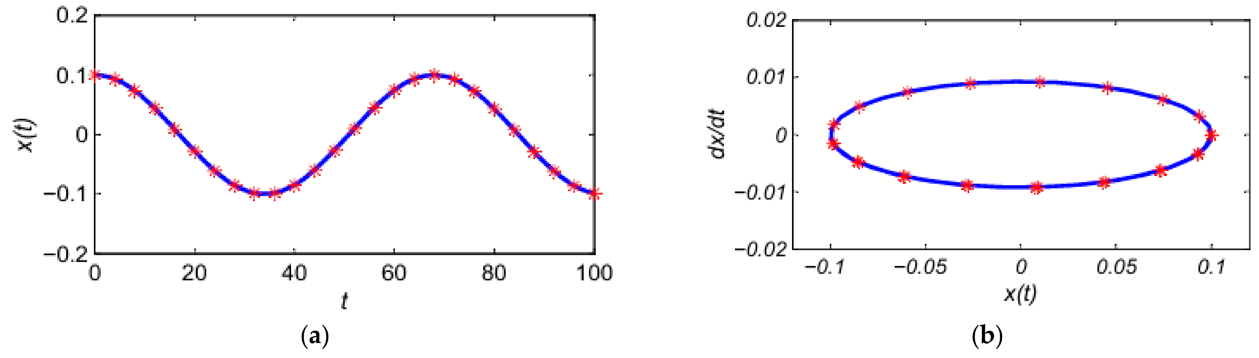
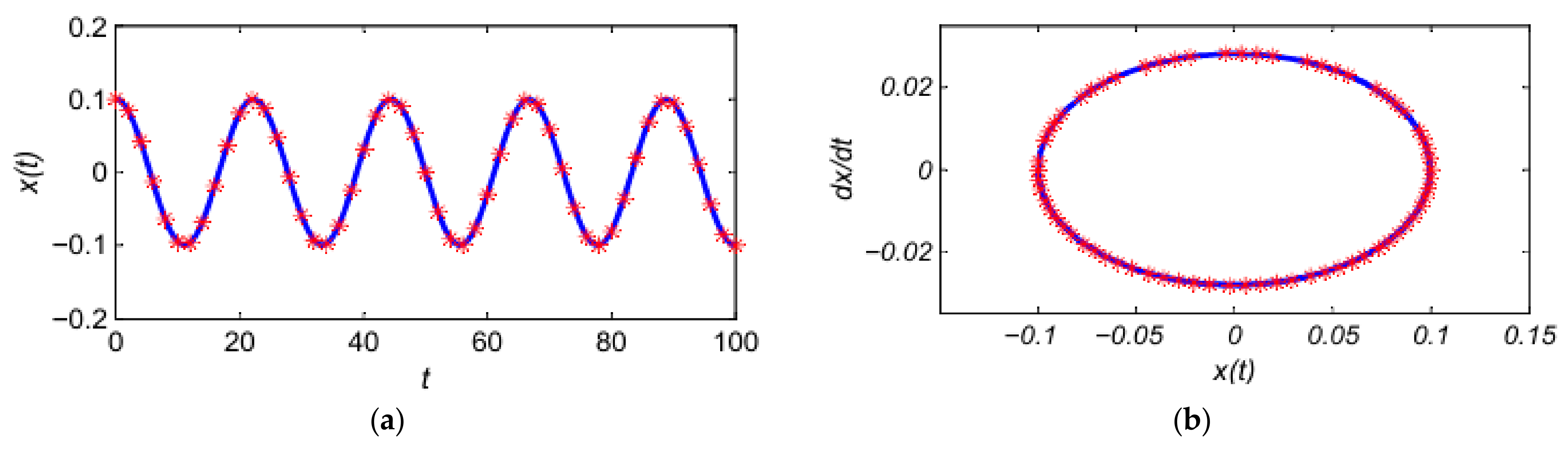
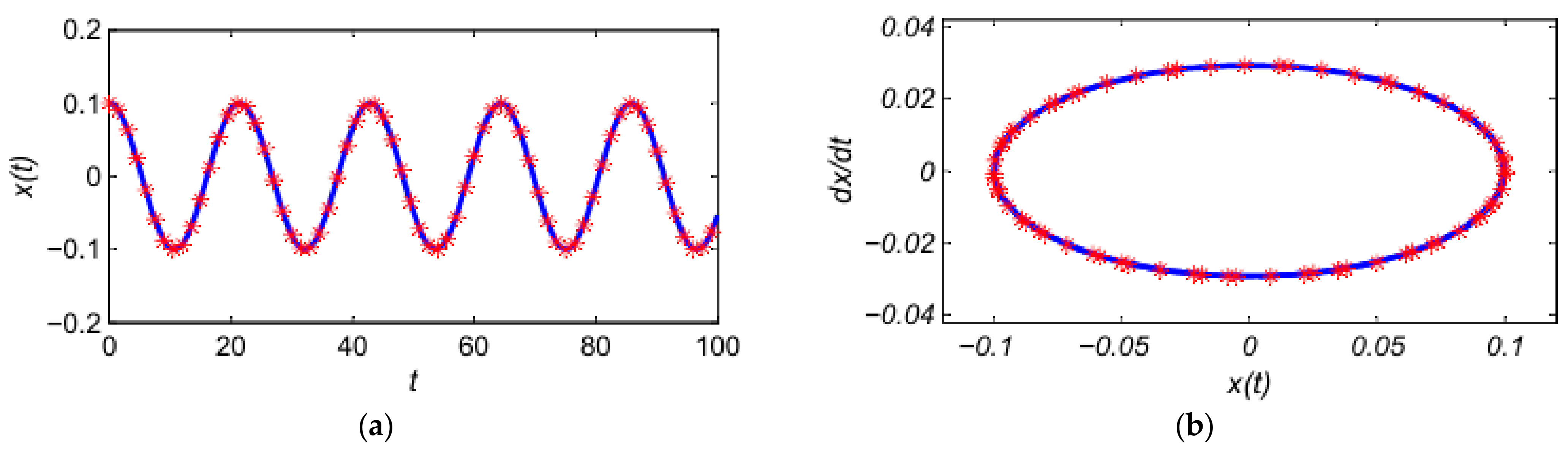
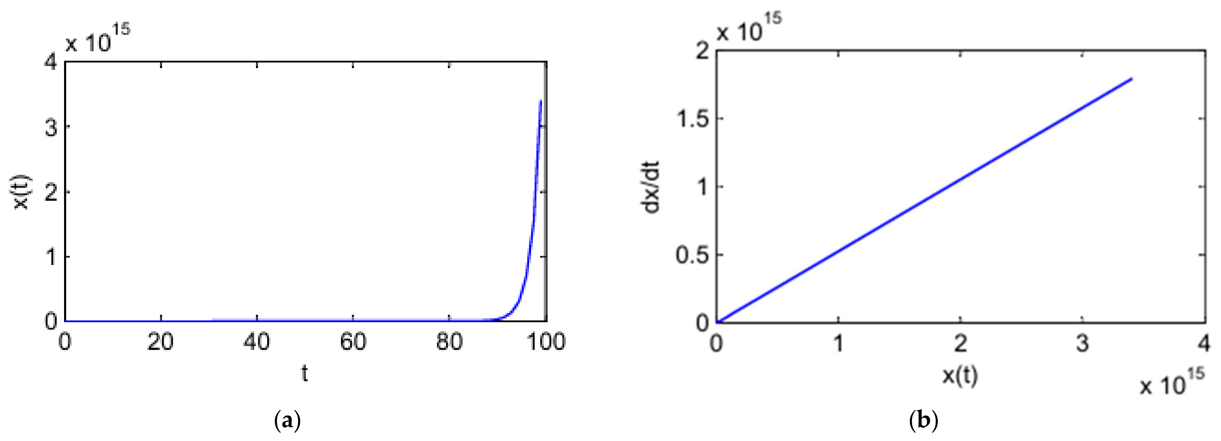
In this section, the numerical behavior of the strongly nonlinear SD oscillator is investigated using time-history responses and phase-plane portraits. To examine the effect of the initial conditions, three cases with different values of the initial displacement are considered: $x\left(0\right)=0.05, \dot{x}\left(0\right)=0$, $x\left(0\right)=0.1, \dot{x}\left(0\right)=0$, and $x\left(0\right)=0.15, \dot{x}\left(0\right)=0$, as illustrated in Figure 2. The obtained results clearly demonstrate the sensitivity of the oscillator response to variations in the initial displacement. It is observed that increasing the initial displacement leads to higher oscillation amplitudes while maintaining the periodic nature of the motion. The phase-plane trajectories further confirm this behavior, where larger initial displacements produce wider closed orbits around the equilibrium position. In addition, a second set of initial conditions with different values of the initial velocity is considered: $x\left(0\right)=0.1, \dot{x}\left(0\right)=0$, $x\left(0\right)=0.1, \dot{x}\left(0\right)=0.1$, and $x\left(0\right)=0.1, \dot{x}\left(0\right)=0.15$, as shown in Figure 3. The numerical results indicate that increasing the initial velocity also increases the response amplitude and enlarges the corresponding phase trajectories. Despite the noticeable influence of both the initial displacement and velocity on the system dynamics, the oscillator remains stable for all considered cases. To further evaluate the effectiveness of the SRHBM and MSM approaches, we solve the initial value problem associated with Equation (9) and compare their first-order approximate solutions with those obtained by the Runge–Kutta method. The analysis is conducted for $A=0.1$ and four parameter combinations: ($k=0.01, \alpha =5$), ($k=0.01, \alpha =7$), ($k=0.1, \alpha =5$), and ($k=0.1, \alpha =7$). Figure 4, Figure 5, Figure 6, Figure 7 and Figure 8 show the SRHBM first-order solutions (red circles) compared with the Runge–Kutta results (blue solid lines). For example, when $k=0.01$, and $\alpha =5$, the frequencies ${\omega }_0=0.0894$ and ${\omega }_{\left(1\right)}=0.089422$ obtained by SRHBM are in close agreement with the MSM frequency of 0.089442271 derived from Equation (44). Across all four cases, the SRHBM solutions exhibit good agreement with the Runge–Kutta method. Furthermore, the phase portraits confirm that the nonlinear SD oscillator admits a stable periodic solution. Figure 9, Figure 10, Figure 11 and Figure 12 present the first-order MSM solutions (red stars) for the same parameter sets. Once again, the results closely match the Runge–Kutta solutions, further validating the accuracy of MSM. Overall, these observations confirm that both SRHBM and MSM are effective analytical tools for approximating the dynamics of strongly nonlinear systems, providing solutions that closely mirror numerical results. The first-order MSM is valid for weak to moderately nonlinear regimes and loses accuracy as nonlinear parameters increase ($0<\alpha <1$). Figure 13 illustrates that the system response reaches a very large amplitude of approximately $4\times {10}^{15}$ (for $\alpha =0.7$), In addition, the phase portrait displays an expanding trajectory, indicating the absence of bounded periodic motion and the emergence of unstable dynamics.

Table 1. Comparison of the approximate solutions with the numerical solution.

Time (t)	${\mathit{x}}_{\mathit{R}\mathit{K}}$	${\mathit{x}}_1$	${\mathit{x}}_1$ (% Error)	${\mathit{x}}_2$	${\mathit{x}}_2$ (% Error)
2	0.08334	0.08334	0	0.08334	0
4	0.03891	0.03891	0	0.03892	0.025700
6	−0.01849	−0.01848	0.040833	−0.01847	0.108167
8	−0.06973	−0.06971	0.028682	−0.06972	0.014341
10	−0.09774	−0.09772	0.020462	−0.09775	0.010231
12	−0.09317	−0.09317	0	−0.09317	0
14	−0.05754	−0.05758	0.069517	−0.05756	0.034758
16	−0.002755	−0.002804	1.77885	−0.002806	1.85118
18	0.05296	0.05291	0.094410	0.05290	0.113293
20	0.09101	0.09099	0.021976	0.09099	0.021976
22	0.09873	0.09876	0.030386	0.09876	0.030386
24	0.07357	0.07362	0.067962	0.07362	0.067962
26	0.02387	0.02396	0.377042	0.02396	0.377042

presents a comparison between the approximate solutions and the numerical Runge–Kutta solution over the investigated time interval. The absolute relative errors of solutions are considered as $\left(\% error\right)=\left|{\displaystyle \frac{x_{RK} - x_m}{x_{RK}}}\right|\times 100$, m = 1, 2. The approximate solutions of the SD oscillator obtained using the SHRPM and MSM methods are denoted by $x_1$ and $x_2$, respectively. The results indicate that both approximation solutions accurately capture the oscillatory behaviour of the system with very small absolute relative errors. For most cases, the percentage error remains below 0.1%, which reflects the accuracy of the adopted approximate approaches.

5. Conclusions

The spreading residue harmonic balance method (SRHBM) and the method of multiple scales (MSM) were employed to investigate the smooth-discontinuous (SD) oscillator. Zero- and first-order approximate solutions were derived for the nonlinear governing equation. The first-order harmonic approximations were presented through time responses and phase portraits for different values of $k$ and $\alpha$, and compared with numerical solutions obtained using the Runge–Kutta method. The comparison presented in Table 1 shows that the approximate solutions obtained by SRHBM and MSM maintain very small relative errors with respect to the numerical results, demonstrating the accuracy of the proposed approaches. Furthermore, the first-order MSM is valid for weak to moderately nonlinear regimes and loses accuracy as nonlinear parameters increase ($0<\alpha <1$). Overall, the obtained results confirm the effectiveness of SRHBM and MSM in describing the dynamics of the nonlinear SD oscillator.

References

1. Tian, Y. Frequency formula for a class of fractal vibration system. Rep. Mech. Eng. 2022, 3, 55–61. [Google Scholar] [CrossRef] [Scilit]
2. He, J.H.; Yang, Q.; He, C.H.; Khan, Y. A simple frequency formulation for the tangent oscillator. Axioms 2021, 10, 320. [Google Scholar] [CrossRef] [Scilit]
3. Anjum, N.; He, J.H. Higher-order homotopy perturbation method for conservative nonlinear oscillators generally and microelectromechanical systems’ oscillators particularly. Int. J. Mod. Phys. B 2020, 34, 2050313. [Google Scholar] [CrossRef] [Scilit]
4. He, J.H.; Amer, T.S.; Elnaggar, S.; Galal, A.A. Periodic property and instability of a rotating pendulum system. Axioms 2021, 10, 191. [Google Scholar] [CrossRef] [Scilit]
5. Abouelregal, A.E.; Mohammad-Sedighi, H.; Faghidian, S.A.; Shirazi, A.H. Temperature-dependent physical characteristics of the rotating nonlocal nanobeams subject to a varying heat source and a dynamic load. Facta Univ. Ser. Mech. Eng. 2021, 19, 633–656. [Google Scholar] [CrossRef] [Scilit]
6. Sedighi, H.M.; Shirazi, K.H. Dynamic pull-in instability of double-sided actuated nano-torsional switches. Acta Mech. Solida Sin. 2015, 28, 91–101. [Google Scholar] [CrossRef] [Scilit]
7. El-Salam, M.A.; Hussein, R.K. Reducing the Primary Resonance Vibrations of a Cantilever Beam Using a Proportional Fractional-Order Derivative Controller. Mathematics 2025, 13, 1886. [Google Scholar] [CrossRef] [Scilit]
8. Hosen, M.A.; Chowdhury, M.S.H. A new reliable analytical solution for strongly nonlinear oscillator with cubic and harmonic restoring force. Results Phys. 2015, 5, 111–114. [Google Scholar] [CrossRef] [Scilit]
9. Li, S.; Niu, J.; Li, X. Primary resonance of fractional-order Duffing–van der Pol oscillator by harmonic balance method. Chin. Phys. B 2018, 27, 120502. [Google Scholar] [CrossRef] [Scilit]
10. Amer, Y.A.; EL-Sayed, A.T.; Abd EL-Salam, M.N. On controlling of vibrations of a suspended cable via positive position feedback controller. Int. J. Dyn. Control 2023, 11, 370–384. [Google Scholar] [CrossRef] [Scilit]
11. Meng, Q.; Hou, L.; Lin, R.; Chen, Y.; Cui, G.; Shi, W.; Chen, Y. Accurate nonlinear dynamic characteristics analysis of quasi-zero-stiffness vibration isolator via a modified incremental harmonic balance method. Nonlinear Dyn. 2024, 112, 125–150. [Google Scholar] [CrossRef] [Scilit]
12. Guo, L.; Wang, X.; Fan, R.L.; Bi, F. Review on development of high-static–low-dynamic-stiffness seat cushion mattress for vibration control of seating suspension system. Appl. Sci. 2020, 10, 2887. [Google Scholar] [CrossRef] [Scilit]
13. Liu, C.; Jing, X.; Daley, S.; Li, F. Recent advances in micro-vibration isolation. Mech. Syst. Signal Process. 2015, 56, 55–80. [Google Scholar] [CrossRef] [Scilit]
14. Li, Z.X.; Cao, Q.J.; Alain, L. Complex dynamics of an archetypal self-excited SD oscillator driven by moving belt friction. Chin. Phys. B 2015, 25, 010502. [Google Scholar] [CrossRef] [Scilit]
15. Abd El-Salam, M.N.; Hussein, R.K.; El-Shourbagy, S.M. Improving Stability and Reducing Vibrations of the Smooth and Discontinuous Oscillator Using a Proportional–Derivative Controller. Axioms 2025, 14, 444. [Google Scholar] [CrossRef] [Scilit]
16. Amer, Y.A.; Abdullah, R.E.; Khaled, O.M.; Mahdy, A.M.S.; Abd El-Salam, M.N. Vibration control of smooth and discontinuous oscillator via negative derivative feedback. J. Vib. Eng. Technol. 2024, 12, 2351–2363. [Google Scholar] [CrossRef] [Scilit]
17. Semler, C.; Gentleman, W.C.; Paıdoussis, M.P. Numerical solutions of second order implicit non-linear ordinary differential equations. J. Sound Vib. 1996, 195, 553–574. [Google Scholar] [CrossRef] [Scilit]
18. Lai, S.K.; Lim, C.W.; Wu, B.S.; Wang, C.; Zeng, Q.C.; He, X. Newton–harmonic balancing approach for accurate solutions to nonlinear cubic–quintic Duffing oscillators. Appl. Math. Model. 2009, 33, 852–866. [Google Scholar] [CrossRef] [Scilit]
19. Leung, A.Y.T.; Guo, Z. Residue harmonic balance for two-degree-of-freedom airfoils with cubic structural nonlinearity. AIAA J. 2011, 49, 2607–2615. [Google Scholar] [CrossRef] [Scilit]
20. Guo, Z.; Leung, A.Y.T.; Yang, H.X. Oscillatory region and asymptotic solution of fractional van der Pol oscillator via residue harmonic balance technique. Appl. Math. Model. 2011, 35, 3918–3925. [Google Scholar] [CrossRef] [Scilit]
21. Leung, A.Y.T.; Guo, Z. Residue harmonic balance approach to limit cycles of non-linear jerk equations. Int. J. Non-Linear Mech. 2011, 46, 898–906. [Google Scholar] [CrossRef] [Scilit]
22. Mickens, R.E. A generalization of the method of harmonic balance. J. Sound Vib. 1986, 111, 515–518. [Google Scholar] [CrossRef] [Scilit]
23. Mickens, R.E. Truly Nonlinear Oscillations: Harmonic Balance, Parameter Expansions, Iteration, and Averaging Methods; World Scientific: Singapore, 2010. [Google Scholar]
24. Anjum, N.; He, J.H.; Ain, Q.T.; Tian, D. Li-He’s modified homotopy perturbation method for doubly-clamped electrically actuated microbeams-based microelectromechanical system. Facta Univ. Ser. Mech. Eng. 2021, 19, 601–612. [Google Scholar] [CrossRef] [Scilit]
25. Lu, J. Global residue harmonic balance method for strongly nonlinear oscillator with cubic and harmonic restoring force. J. Low Freq. Noise Vib. Act. Control 2022, 41, 1402–1410. [Google Scholar] [CrossRef] [Scilit]
26. Qian, Y.H.; Pan, J.L.; Qiang, Y.; Wang, J.S. The spreading residue harmonic balance method for studying the doubly clamped beam-type N/MEMS subjected to the van der Waals attraction. J. Low Freq. Noise Vib. Act. Control 2019, 38, 1261–1271. [Google Scholar] [CrossRef] [Scilit]
27. Liu, Y.; Vella, D.; Qin, Z.; Chu, F.; Amabili, M. A review of nonlinear dynamics and vibration in lightweight composite structures: Recent advances and challenges. Eng. Struct. 2026, 360, 122835. [Google Scholar] [CrossRef] [Scilit]
28. Amer, Y.A.; Hussein, R.K.; Abu Alrub, S.; Elgazzar, A.S.; Salman, T.M.; Mousa, F.; Abd El-Salam, M.N. Suppressing Nonlinear Resonant Vibrations via NINDF Control in Beam Structures. Mathematics 2025, 13, 2137. [Google Scholar] [CrossRef] [Scilit]
29. Amer, Y.A.; El-Sayed, A.T.; Agwa, M.M. Controlling wind turbine tower vibration under external force by applying control systems combination. Sci. Rep. 2024, 14, 18597. [Google Scholar] [CrossRef] [Scilit]
30. Bauomy, H.S.; EL-Sayed, A.T.; Amer, T.S.; Abohamer, M.K. Negative derivative feedback control and bifurcation in a two-degree-of-freedom coupled dynamical system. Chaos Solitons Fractals 2025, 193, 116138. [Google Scholar] [CrossRef] [Scilit]
31. Bauomy, H.S.; El-Sayed, A.T.; El-Bahrawy, F.T.; Salem, A.M. Safety of a continuous spinning Shaft’s structure from nonlinear vibration with NIPPF. Alex. Eng. J. 2023, 67, 193–207. [Google Scholar] [CrossRef] [Scilit]
32. Saeed, N.A.; El-Shourbagy, S.M.; Kamel, M.; Raslan, K.R.; Aboudaif, M.K. Nonlinear dynamics and static bifurcations control of the 12-pole magnetic bearings system utilizing the integral resonant control strategy. J. Low Freq. Noise Vib. Act. Control 2022, 41, 1532–1560. [Google Scholar] [CrossRef] [Scilit]
33. Thompson, J.M.T. Basic principles in the general theory of elastic stability. J. Mech. Phys. Solids 1963, 11, 13–20. [Google Scholar] [CrossRef] [Scilit]
34. Savi, M.A.; Pacheco, P.M.C.L. Transient chaos in an elasto-plastic beam with hardening. J. Braz. Soc. Mech. Sci. Eng. 2003, 25, 189–193. [Google Scholar] [CrossRef] [Scilit]
35. Cao, Q.; Léger, A.; Wiercigroch, M. A Smooth and Discontinuous Oscillator; Springer Tracts in Mechanical Engineering: Berlin/Heidelberg, Germany, 2016. [Google Scholar]
36. Guo, Z.; Leung, A.Y.T.; Ma, X. Solution procedure of residue harmonic balance method and its applications. Sci. China Phys. Mech. Astron. 2014, 57, 1581–1591. [Google Scholar] [CrossRef] [Scilit]
37. Momani, S.; Erjaee, G.H.; Alnasr, M.H. The modified homotopy perturbation method for solving strongly nonlinear oscillators. Comput. Math. Appl. 2009, 58, 2209–2220. [Google Scholar] [CrossRef] [Scilit]
38. Urabe, M. Galerkin’s procedure for nonlinear periodic systems. Arch. Ration. Mech. Anal. 1964, 20, 120–152. [Google Scholar] [CrossRef] [Scilit]
39. Nayfeh, A.H. Problems in perturbation. Appl. Opt. 1986, 25, 3145. [Google Scholar]
40. Nayfeh, A.H.; Mook, D.T. Nonlinear Oscillations; John Wiley: New York, NY, USA, 1985. [Google Scholar]
Figure 1. The SD oscillator schematic, (a) for α > 0 and (b) for α = 0 .
Mathematics 14 01687 g001
Figure 2. The influence of initial displacement conditions on the SD oscillator: (a) the time response and (b) the phase plane.
Mathematics 14 01687 g002
Figure 3. The influence of initial velocity conditions on the SD oscillator: (a) the time response and (b) the phase plane.
Mathematics 14 01687 g003
Figure 4. First-order SRHBM versus Runge–Kutta results for k = 0.01 ,   α = 5 (a) the time response, and (b) the phase plane.
Mathematics 14 01687 g004
Figure 5. First-order SRHBM versus Runge–Kutta results for k = 0.01 ,   α = 7 . (a) the time response, and (b) the phase plane.
Mathematics 14 01687 g005
Figure 6. First-order SRHBM versus Runge–Kutta results for k = 0.1 ,   α = 5 . (a) the time response, and (b) the phase plane.
Mathematics 14 01687 g006
Figure 7. First-order SRHBM versus Runge–Kutta results for k = 0.1 ,   α = 7 . (a) the time response, and (b) the phase plane.
Mathematics 14 01687 g007
Figure 8. First-order SRHBM versus Runge–Kutta results for k = 0.05 ,   α = 5 . (a) the time response, and (b) the phase plane.
Mathematics 14 01687 g008
Figure 9. First-order MSM versus Runge–Kutta results for k = 0.01 ,   α = 5 . (a) the time response, and (b) the phase plane.
Mathematics 14 01687 g009
Figure 10. First-order MSM versus Runge–Kutta results for k = 0.01 ,   α = 7 . (a) the time response, and (b) the phase plane.
Mathematics 14 01687 g010
Figure 11. First-order MSM versus Runge–Kutta results for k = 0.1 ,   α = 5 . (a) the time response, and (b) the phase plane.
Mathematics 14 01687 g011
Figure 12. First-order MSM versus Runge–Kutta results for k = 0.1 ,   α = 7 . (a) the time response, and (b) the phase plane.
Mathematics 14 01687 g012
Figure 13. First-order MSM for k = 0.1 ,   α = 0.7 . (a) the time response, and (b) the phase plane.
Mathematics 14 01687 g013